


1 Introduction
First passage percolation (FPP) is a natural way to understand geodesics in random metric spaces. Starting from some initial vertex at time
 $0$
, the process spreads through the underlying graph so that the transmission time between any two vertices
$0$
, the process spreads through the underlying graph so that the transmission time between any two vertices
 $x,y$
is the minimum sum of edge transmission times over all paths between x and y. In classical FPP, edge transmission times are independent and identically distributed random variables. In the recent paper [Reference Komjáthy, Lapinskas and Lengler55] we introduced one-dependent FPP, where edge transmission times depend on the edge’s direct surroundings in the underlying graph. There, we determined the phase transition for explosion (i.e., reaching infinitely many vertices in finite time). In this paper we study the sub-explosive regime, when explosion does not occur. We show that the process exhibits rich behaviour with several growth phases and nonsmooth phase transitions between them. This holds across a large class of scale-free spatial random graph models (namely Scale-Free Percolation (SFP), Hyperbolic Random Graphs (HypRG), and infinite and finite Geometric Inhomogeneous Random Graphs (GIRG) [Reference Deijfen, van der Hofstad and Hooghiemstra26, Reference Bringmann, Keusch and Lengler17, Reference Krioukov, Papadopoulos, Kitsak, Vahdat and Boguná58]), and across all Markovian and non-Markovian transmission time distributions with reasonable limiting behaviour at zero.
$x,y$
is the minimum sum of edge transmission times over all paths between x and y. In classical FPP, edge transmission times are independent and identically distributed random variables. In the recent paper [Reference Komjáthy, Lapinskas and Lengler55] we introduced one-dependent FPP, where edge transmission times depend on the edge’s direct surroundings in the underlying graph. There, we determined the phase transition for explosion (i.e., reaching infinitely many vertices in finite time). In this paper we study the sub-explosive regime, when explosion does not occur. We show that the process exhibits rich behaviour with several growth phases and nonsmooth phase transitions between them. This holds across a large class of scale-free spatial random graph models (namely Scale-Free Percolation (SFP), Hyperbolic Random Graphs (HypRG), and infinite and finite Geometric Inhomogeneous Random Graphs (GIRG) [Reference Deijfen, van der Hofstad and Hooghiemstra26, Reference Bringmann, Keusch and Lengler17, Reference Krioukov, Papadopoulos, Kitsak, Vahdat and Boguná58]), and across all Markovian and non-Markovian transmission time distributions with reasonable limiting behaviour at zero.
In SFP, the vertex set is formed by the d-dimensional lattice
 $\mathbb {Z}^d$
. Each vertex u is then equipped with an independent and identically distributed random vertex-weight
$\mathbb {Z}^d$
. Each vertex u is then equipped with an independent and identically distributed random vertex-weight
 $W_u\ge 1$
. Given the weighted vertex set, the edges are drawn conditionally independently. The probability of an edge between vertices
$W_u\ge 1$
. Given the weighted vertex set, the edges are drawn conditionally independently. The probability of an edge between vertices
 $u, v$
with weights
$u, v$
with weights
 $W_u, W_v$
decreases with the Euclidean distance
$W_u, W_v$
decreases with the Euclidean distance
 $|u-v|$
and increases with the vertex-weights, and is between constant factors of
$|u-v|$
and increases with the vertex-weights, and is between constant factors of
 $\min (1, W_u W_v/|u-v|^d)^\alpha $
, see Definition 1.3 below for full detail. The parameter
$\min (1, W_u W_v/|u-v|^d)^\alpha $
, see Definition 1.3 below for full detail. The parameter
 $\alpha $
is often called the long-range parameter, since the model with all vertex-weights set to
$\alpha $
is often called the long-range parameter, since the model with all vertex-weights set to
 $1$
recovers the classical long-range percolation model [Reference Schulman72]. Instead of unit vertex-weights, here we shall rather assume that the vertex-weight distribution W follows a regularly varying tail, that is, for some
$1$
recovers the classical long-range percolation model [Reference Schulman72]. Instead of unit vertex-weights, here we shall rather assume that the vertex-weight distribution W follows a regularly varying tail, that is, for some
 $\tau \in (2,3)$
that is called the power-law exponent we assume
$\tau \in (2,3)$
that is called the power-law exponent we assume
 $$ \begin{align} \frac{\mathbb{P}(W\ge x)}{\mathbb{P}(W\ge cx)} \to c^{-(\tau-1)} \qquad \text{ for all } c>0 \text{ as } x\to \infty. \end{align} $$
The heavy-tailed decay of W creates degree-inhomogeneity in the model: the vertex weight
 $W_v$
of v is (up to constant factors) equal to the expected degree of v, and the degree of a high-weight vertex is concentrated around its expectation [Reference Deijfen, van der Hofstad and Hooghiemstra26, Proposition 2.3]. The parameters
$W_v$
of v is (up to constant factors) equal to the expected degree of v, and the degree of a high-weight vertex is concentrated around its expectation [Reference Deijfen, van der Hofstad and Hooghiemstra26, Proposition 2.3]. The parameters
 $\tau , \alpha $
play different roles in governing inhomogeneities in the models: while
$\tau , \alpha $
play different roles in governing inhomogeneities in the models: while
 $\tau $
governs the degree distribution, a smaller
$\tau $
governs the degree distribution, a smaller
 $\alpha $
causes a heavier tail on the edge-length distribution, with
$\alpha $
causes a heavier tail on the edge-length distribution, with
 $\alpha>1$
needed for a.s. finite degrees [Reference Deijfen, van der Hofstad and Hooghiemstra26]. The model GIRG follows the same construction by replacing the location of vertices by a unit-intensity Poisson point process (PPP) on
$\alpha>1$
needed for a.s. finite degrees [Reference Deijfen, van der Hofstad and Hooghiemstra26]. The model GIRG follows the same construction by replacing the location of vertices by a unit-intensity Poisson point process (PPP) on
 $\mathbb {R}^d$
. For the overview of the results, the reader may ignore this difference.
$\mathbb {R}^d$
. For the overview of the results, the reader may ignore this difference.
Universality classes of transmission times. In one-dependent first passage percolation, we set the transmission time through the edge
 $e=xy$
between vertices
$e=xy$
between vertices
 $x,y$
as the product of an independent and identically distributed (i.i.d.) random factor
$x,y$
as the product of an independent and identically distributed (i.i.d.) random factor
 $L_{xy}$
and a factor depending on the weights of vertices:
$L_{xy}$
and a factor depending on the weights of vertices:
Definition 1.1 (1-dependent first passage percolation (1-FPP)).
Consider a graph
 $G = (\mathcal {V}, \mathcal {E})$
where each vertex
$G = (\mathcal {V}, \mathcal {E})$
where each vertex
 $v\in \mathcal {V}$
has an associated vertex-weight
$v\in \mathcal {V}$
has an associated vertex-weight
 $W_v$
. For every edge
$W_v$
. For every edge
 $xy\in \mathcal {E}$
, draw an i.i.d. copy
$xy\in \mathcal {E}$
, draw an i.i.d. copy
 $L_{xy}$
of a random variable L, and set the (transmission) cost of an edge
$L_{xy}$
of a random variable L, and set the (transmission) cost of an edge
 $xy$
as
$xy$
as
 $$ \begin{align} \mathcal{C}(xy):=L_{xy}(W_xW_y)^{\mu}, \end{align} $$
for a fixed parameter
 $\mu>0$
called the penalty strength. The costs define a cost distance
$\mu>0$
called the penalty strength. The costs define a cost distance
 $d_{\mathcal {C}}(x,y)$
between any two vertices x and y, which is the minimal total cost of any path between x and y (see Section 1.4.1). We call
$d_{\mathcal {C}}(x,y)$
between any two vertices x and y, which is the minimal total cost of any path between x and y (see Section 1.4.1). We call
 $d_{\mathcal {C}}$
the 1-dependent first passage percolation.
$d_{\mathcal {C}}$
the 1-dependent first passage percolation.
We usually assume that the cumulative distribution function (cdf)
 $F_L:[0,\infty )\rightarrow [0,1]$
of L satisfies the following assumption (with exceptions of this assumption explicitly mentioned):
$F_L:[0,\infty )\rightarrow [0,1]$
of L satisfies the following assumption (with exceptions of this assumption explicitly mentioned):
Assumption 1.2. There exist constants
 $t_0,\,c_1,\,c_2,\,\beta>0$
such that
$t_0,\,c_1,\,c_2,\,\beta>0$
such that
 $$ \begin{align} c_1t^{\beta}\le F_L(t)\le c_2t^{\beta}\text{ for all }t\in[0,t_0]. \end{align} $$
Without much effort, one can relax Assumption 1.2 to
 $\lim _{x\to 0} \log F_L(x)/\log x=\beta $
, that is, regularly varying behaviour of
$\lim _{x\to 0} \log F_L(x)/\log x=\beta $
, that is, regularly varying behaviour of
 $F_L$
near
$F_L$
near
 $0$
. We work with (1.3) for the sake of readability. Table 1 provides an overview of the various parameters of the model.
$0$
. We work with (1.3) for the sake of readability. Table 1 provides an overview of the various parameters of the model.
Summary and brief description of the main parameters of the model.

The cost distance
 $d_{\mathcal {C}}(x,y)$
corresponds to the transmission time between two vertices
$d_{\mathcal {C}}(x,y)$
corresponds to the transmission time between two vertices
 $x,y$
. In SFP, we use the same vertex weights
$x,y$
. In SFP, we use the same vertex weights
 $W_x,W_y$
to generate the edge between
$W_x,W_y$
to generate the edge between
 $x,y$
as well as to define the edge-cost
$x,y$
as well as to define the edge-cost
 $\mathcal {C}(xy)$
. This leads to the cost of the edge to depend essentially on the expected degrees of the two involved verticesFootnote
1
, however, it also leads to three layers of randomness. On the first layer, the vertex set has random vertex-weights; on the second layer, edges are drawn randomly using the randomness in the first layer, and finally, on the third layer, edge-costs depend on the presence of edges, on the vertex-weights, and on an extra source of randomness captured in
$\mathcal {C}(xy)$
. This leads to the cost of the edge to depend essentially on the expected degrees of the two involved verticesFootnote
1
, however, it also leads to three layers of randomness. On the first layer, the vertex set has random vertex-weights; on the second layer, edges are drawn randomly using the randomness in the first layer, and finally, on the third layer, edge-costs depend on the presence of edges, on the vertex-weights, and on an extra source of randomness captured in
 $L_{xy}$
.
$L_{xy}$
.
When
 $\mu \in (0,1)$
, a high-degree vertex still causes more new infections per unit time than a low-degree vertex, but this effect is sublinear in the degree. As
$\mu \in (0,1)$
, a high-degree vertex still causes more new infections per unit time than a low-degree vertex, but this effect is sublinear in the degree. As
 $\mu $
increases and/or the parameters of the underlying graph change, we prove that the following four different phases occur for the transmission time between the vertex at
$\mu $
increases and/or the parameters of the underlying graph change, we prove that the following four different phases occur for the transmission time between the vertex at
 $0$
and a far away vertex x, see Table 2 for the thresholds between the different phases:
$0$
and a far away vertex x, see Table 2 for the thresholds between the different phases:
-
(i)
 $d_{\mathcal {C}}(0,x)$
converges to a limiting distribution that is independent of the Euclidean distance
$|x|$
(explosive phase);
$d_{\mathcal {C}}(0,x)$
converges to a limiting distribution that is independent of the Euclidean distance
$|x|$
(explosive phase);


This was the main result of [Reference Komjáthy, Lapinskas and Lengler55]. The main result of this paper is to characterise the other phases:
-
(ii)
$d_{\mathcal {C}}(0,x)$
grows at most polylogarithmically in the Euclidean distance
$|x|$
, without being explosive; -
(iii)
$d_{\mathcal {C}}(0,x)$
grows polynomially in
$|x|$
, with exponent
$0<\eta _0 < 1$
; -
(iv)
$d_{\mathcal {C}}(0,x)$
grows linearly in
$|x|$
, that is, with exponent
$\eta _0=1$
.


These phases are highly robust in the parameters, they are not restricted to phase boundaries in either
 $\mu $
or the other model parameters. Moreover, all four phases can occur on a single underlying graph by changing the penalty exponent
$\mu $
or the other model parameters. Moreover, all four phases can occur on a single underlying graph by changing the penalty exponent
 $\mu $
only; universally across distributions of
$\mu $
only; universally across distributions of
 $L_{xy}$
with regularly varying behaviour at
$L_{xy}$
with regularly varying behaviour at
 $0$
, see Figure 1 for a visualisation. This rich behaviour arises despite the doubly logarithmic graph distances in the underlying spatial graph models. By contrast, in other models the behaviour of transmission times in classical FPP is less rich, see Section 1.1 for the discussion.
$0$
, see Figure 1 for a visualisation. This rich behaviour arises despite the doubly logarithmic graph distances in the underlying spatial graph models. By contrast, in other models the behaviour of transmission times in classical FPP is less rich, see Section 1.1 for the discussion.
Summary of our main results. In 1-FPP, edge transmission times are
 $L_{xy} (W_xW_y)^\mu $
where
$L_{xy} (W_xW_y)^\mu $
where
 $W_x, W_y$
are constant multiples of the expected degrees of the vertices
$W_x, W_y$
are constant multiples of the expected degrees of the vertices
 $x,y$
, and
$x,y$
, and
 $L_{xy}$
is i.i.d. with distribution function that varies regularly near
$L_{xy}$
is i.i.d. with distribution function that varies regularly near
 $0$
with exponent
$0$
with exponent
 $\beta \in (0,\infty ]$
. The degree distribution follows a power law with exponent
$\beta \in (0,\infty ]$
. The degree distribution follows a power law with exponent
 $\tau \in (2,3)$
: graph distances are doubly logarithmic in the underlying graph. The transmission time
$\tau \in (2,3)$
: graph distances are doubly logarithmic in the underlying graph. The transmission time
 $d_{\mathcal {C}}(0,x)$
between
$d_{\mathcal {C}}(0,x)$
between
 $0$
and a far away vertex x sweeps through four different phases as the penalty exponent
$0$
and a far away vertex x sweeps through four different phases as the penalty exponent
 $\mu $
increases. For long-range parameter
$\mu $
increases. For long-range parameter
 $\alpha \in (1,2)$
, long edges between low-degree vertices maintain polylogarithmic transmission times (similar to long-range percolation), so increasing
$\alpha \in (1,2)$
, long edges between low-degree vertices maintain polylogarithmic transmission times (similar to long-range percolation), so increasing
 $\mu $
stops explosion but it has no further effect. When
$\mu $
stops explosion but it has no further effect. When
 $\alpha>2$
, these edges are sparser and a larger
$\alpha>2$
, these edges are sparser and a larger
 $\mu $
slows down 1-FPP, to polynomial but sublinear transmission times in an interval of length at least
$\mu $
slows down 1-FPP, to polynomial but sublinear transmission times in an interval of length at least
 $1/d$
for
$1/d$
for
 $\mu $
. Then, all long edges have polynomial transmission times in the distance they bridge. For even higher penalty exponent
$\mu $
. Then, all long edges have polynomial transmission times in the distance they bridge. For even higher penalty exponent
 $\mu $
the behaviour becomes similar to FPP on the grid
$\mu $
the behaviour becomes similar to FPP on the grid
 $\mathbb {Z}^d$
. We give the growth exponents
$\mathbb {Z}^d$
. We give the growth exponents
 $\Delta _0$
and
$\Delta _0$
and
 $\eta _0$
explicitly in (1.9) and (1.10).
$\eta _0$
explicitly in (1.9) and (1.10).

Heatmaps for the four different universality classes. The vertices are sorted by their transmission times from the origin (centre vertex). The colours represent this ordering: yellow infected first, then orange, then purple. All four plots are generated on the same underlying graph (with parameters
 $\tau =2.3$
and
$\tau =2.3$
and
 $\alpha =5$
, and edge connection probabilities
$\alpha =5$
, and edge connection probabilities
 $p(u,v)=(w_u w_v / (\mathbb {E}[W]\|u-v\|^2))^5 \wedge 1$
), where the vertices are placed on a
$p(u,v)=(w_u w_v / (\mathbb {E}[W]\|u-v\|^2))^5 \wedge 1$
), where the vertices are placed on a
 $750 \times 750$
grid in the 2-dimensional torus. The random factors
$750 \times 750$
grid in the 2-dimensional torus. The random factors
 $L_{xy}$
associated to each edge are also identical in all four plots, and follow an exponential distribution (i.e.,
$L_{xy}$
associated to each edge are also identical in all four plots, and follow an exponential distribution (i.e.,
 $\beta =1$
). The only varying parameter is the penalty exponent
$\beta =1$
). The only varying parameter is the penalty exponent
 $\mu $
, taking values (i)
$\mu $
, taking values (i)
 $\mu =0$
for the explosive regime, (ii)
$\mu =0$
for the explosive regime, (ii)
 $\mu =0.5$
for the the polylogarithmic regime, (iii)
$\mu =0.5$
for the the polylogarithmic regime, (iii)
 $\mu =1$
for the polynomial regime (iv)
$\mu =1$
for the polynomial regime (iv)
 $\mu =2$
for the linear regime. In the linear regime, the late points are – typically – high degree vertices carrying high penalisation. We thank Zylan Benjert for generating the simulations and the pictures.
$\mu =2$
for the linear regime. In the linear regime, the late points are – typically – high degree vertices carrying high penalisation. We thank Zylan Benjert for generating the simulations and the pictures.

Precise behaviour in the four phases. In this paper we prove the upper bounds on transmission times in the sub-explosive regime (phase (i) was previous work [Reference Komjáthy, Lapinskas and Lengler55]). In phase (ii), we show that the transmission time is at most
 $(\log |x|)^{\Delta _0 + o(1)}$
with an explicit
$(\log |x|)^{\Delta _0 + o(1)}$
with an explicit
 $\Delta _0>1$
which we conjecture to be tight. In phases (iii) and (iv), we show that the transmission time is precisely
$\Delta _0>1$
which we conjecture to be tight. In phases (iii) and (iv), we show that the transmission time is precisely
 $|x|^{\eta _0 \pm o(1)}$
, where we give
$|x|^{\eta _0 \pm o(1)}$
, where we give
 $\eta _0<1$
explicitly for phase (iii) and
$\eta _0<1$
explicitly for phase (iii) and
 $\eta _0 =1$
for phase (iv). The companion paper [Reference Komjáthy, Lapinskas, Lengler and Schaller56] contains the matching lower bounds for phases (iii)-(iv) as well as some additional results for phase (iv). We develop new techniques that allow us to treat upper bounds for all three sub-explosive phases simultaneously, which we expect to be of independent interest.
$\eta _0 =1$
for phase (iv). The companion paper [Reference Komjáthy, Lapinskas, Lengler and Schaller56] contains the matching lower bounds for phases (iii)-(iv) as well as some additional results for phase (iv). We develop new techniques that allow us to treat upper bounds for all three sub-explosive phases simultaneously, which we expect to be of independent interest.
The budget travel plan with 3-edge bridging-paths: (a) first and (b) second iteration.

Motivation of the process from applications. One-dependent processes in general, and one-dependent FPP in particular, allow for more realistic modelling of real phenomena. In social networks, actual contacts and infections do not scale linearly with the degree [Reference Feldman and Janssen31, Reference Kroy59, Reference Wang, Xiong, Wang, Cai, Wu, Wang and Chen76, Reference Ke, Zitzmann, Ho, Ribeiro and Perelson54]. 1-FPP type penalisation has frequently been used to model the sublinear impact of superspreaders [Reference Giuraniuc, Hatchett, Indekeu, Leone, Castillo, Van Schaeybroeck and Vanderzande37, Reference Karsai, Juhász and Iglói53, Reference Miritello, Moro, Lara, Martínez-López, Belchamber, Roberts and Dunbar65, Reference Pu, Li and Yang69, Reference Yang, Zhou, Xie, Lai and Wang77, Reference Baxter and Timár6], and in other contexts [Reference Bonaventura, Nicosia and Latora16, Reference Ding and Li30, Reference Lee, Yook and Kim62, Reference Zlatić, Gabrielli and Caldarelli78, Reference Andrade, Andrade and Herrmann3, Reference Hooyberghs, Van Schaeybroeck, Moreira, Andrade, Herrmann and Indekeu49]. Consistent with our model, all these applications assume a polynomial dependence with exponent in the range
 $\mu \in (0,1)$
, where a high-degree vertex may cause more new infections per time than a low-degree vertex, but this effect is sublinear in the degree.
$\mu \in (0,1)$
, where a high-degree vertex may cause more new infections per time than a low-degree vertex, but this effect is sublinear in the degree.
While our paper is theoretical, we do believe that a model with a rich phase space can have practical implications. In the spread of physical epidemics, while some diseases spread at an exponential rate, others spread at a polynomial rate, dominated by the local geometry. Examples of the latter include HIV/AIDS, Ebola, and foot-and-mouth disease, see the survey [Reference Chowell, Bansal, Sattenspiel and Viboud21] on polynomial epidemic growth. Classical epidemic models can typically only model either exponential or polynomial growth, not both. Arguably,
 $1$
-FPP provides a natural explanation, since in
$1$
-FPP provides a natural explanation, since in
 $1$
-FPP the transition can be driven by changes only to the transmission dynamics, not to the underlying network.
$1$
-FPP the transition can be driven by changes only to the transmission dynamics, not to the underlying network.
New methodology: moving to quenched vertex-set to replace FKG-inequality. In this paper we develop a general technique – nets combined with multiround exposure – that replaces the FKG-inequality [Reference Fortuin, Kasteleyn and Ginibre32] in problems concerning vertex and/or edge-weighted graph models where this inequality does not hold. Let us explain why the FKG-inequality fails in the context of 1-FPP. Typically, for upper bounds one constructs paths connecting
 $0$
and x by revealing vertices and/or edges of the graph sequentially, which destroys the independence of edges. For graph distances in long-range percolation, the FKG-inequality resolves this problem [Reference Biskup11], but it already needs adjustments once vertex-weights are present [Reference Gracar, Lüchtrath and Mönch41]. In 1-FPP, the existence of a long edge is positively correlated to its endpoints having large vertex weights, which is negatively correlated to its other outgoing edges having short transmission times. Hence, having chosen a long edge with low-cost, we lose probabilistic control over how to choose the next low-cost edge on the path connecting
$0$
and x by revealing vertices and/or edges of the graph sequentially, which destroys the independence of edges. For graph distances in long-range percolation, the FKG-inequality resolves this problem [Reference Biskup11], but it already needs adjustments once vertex-weights are present [Reference Gracar, Lüchtrath and Mönch41]. In 1-FPP, the existence of a long edge is positively correlated to its endpoints having large vertex weights, which is negatively correlated to its other outgoing edges having short transmission times. Hence, having chosen a long edge with low-cost, we lose probabilistic control over how to choose the next low-cost edge on the path connecting
 $0$
and x. To overcome this issue, we move to the (weighted-vertex) quenched setting where we reveal the realisation of the whole weighted vertex set – say
$0$
and x. To overcome this issue, we move to the (weighted-vertex) quenched setting where we reveal the realisation of the whole weighted vertex set – say
 $(\mathcal {V}, \mathcal {W})=(V, w_V)$
– and thus events concerning only edges become independent. We show that in a large box centred at the origin of
$(\mathcal {V}, \mathcal {W})=(V, w_V)$
– and thus events concerning only edges become independent. We show that in a large box centred at the origin of
 $\mathbb {R}^d$
, the proportion of realisations with behaviour ‘close to what is expected’ tends to
$\mathbb {R}^d$
, the proportion of realisations with behaviour ‘close to what is expected’ tends to
 $1$
with the box-size. More precisely, we require that locally around a constant proportion of the vertices and uniformly across multiple scales of vertex-weights, the number of points in the weighted vertex set is close to its expectation. For this we select a subset of the vertices that we call a net realising this property. A net
$1$
with the box-size. More precisely, we require that locally around a constant proportion of the vertices and uniformly across multiple scales of vertex-weights, the number of points in the weighted vertex set is close to its expectation. For this we select a subset of the vertices that we call a net realising this property. A net
 $\mathcal {N}$
is thus a subset of the weighted vertex set, such that for every not-too-small radius r, every ‘reasonable’ weight w, and every selected vertex
$\mathcal {N}$
is thus a subset of the weighted vertex set, such that for every not-too-small radius r, every ‘reasonable’ weight w, and every selected vertex
 $v\in \mathcal {N}$
, the net has constant density in
$v\in \mathcal {N}$
, the net has constant density in
 $B_r(v)\times [w, 2w]$
, shorthand for vertices of weight in
$B_r(v)\times [w, 2w]$
, shorthand for vertices of weight in
 $[w,2w]$
within Euclidean distance r of v:
$[w,2w]$
within Euclidean distance r of v:
 $$ \begin{align} \frac{|\mathcal{N}\cap B_r(v)\times[w, 2w]|}{\mathbb{E}\big[|\mathcal{V} \cap B_r(v)\times [w,2w]|\mid v\in \mathcal{V}\big]} \in \Big(\frac{1}{16}, 16\Big), \end{align} $$
where the expectation is taken over the randomness in the weights and location of verticesFootnote
2
. We prove via a multiscale analysis that as the box-size tends to infinity, asymptotically almost every realisation of the weighted vertex set contains a net
 $\mathcal N$
with total density at least
$\mathcal N$
with total density at least
 $1/4$
.
$1/4$
.
When we move to the quenched setting we only reveal the realisation of the weighted vertex set, but not the edges of the graph. In realisations containing a net, with a carefully chosen multiround exposure process we can define a coupling of the edges and their costs which lets us replace the FKG inequality needed for the construction of a low-cost path between
 $0 $
and x, see Section 3 for more details. We believe that this method is also useful for many other graph models, so we explain it streamlined now.
$0 $
and x, see Section 3 for more details. We believe that this method is also useful for many other graph models, so we explain it streamlined now.
Budget travel plan with 3-edge bridge-paths. Switching to the quenched setting allows to prove the upper bounds in all subexponential phases (ii)–(iv) all-at-once. Our construction of a connecting path overcomes the following problem: A long edge with a short transmission time typically occurs on typical high-degree vertices and thus all other outgoing edges from the same vertices have too long transmission times. The main idea resembles a ‘budget travel plan’: when someone travels with a low budget, one takes the cheapest mode of transport to the airport within a
 $100$
km radius that offers the cheapest flight landing within a
$100$
km radius that offers the cheapest flight landing within a
 $100$
km radius of the destination, then takes the cheapest transport to the destination city.
$100$
km radius of the destination, then takes the cheapest transport to the destination city.
Formally, we put balls of radius
 $|x|^\gamma $
for some
$|x|^\gamma $
for some
 $\gamma \in (0,1)$
around
$\gamma \in (0,1)$
around
 $0$
and around x, and we find a cheap
$0$
and around x, and we find a cheap
 $3$
-edge path (‘bridge’)
$3$
-edge path (‘bridge’)
 $\pi _1 = y_0aby_x$
between these two balls using only vertices in the net. The net guarantees enough vertices in each vertex-weight range of interest. We find atypical high-weight vertices
$\pi _1 = y_0aby_x$
between these two balls using only vertices in the net. The net guarantees enough vertices in each vertex-weight range of interest. We find atypical high-weight vertices
 $a,b$
that are connected by an atypically cheap edge, that simultaneously have an atypically cheap edge to low-weight vertices
$a,b$
that are connected by an atypically cheap edge, that simultaneously have an atypically cheap edge to low-weight vertices
 $y_0, y_x$
, respectively. (Here we use the common terminology of fast transmission corresponding to ‘cheap’ cost.) Then we have replaced the task of connecting
$y_0, y_x$
, respectively. (Here we use the common terminology of fast transmission corresponding to ‘cheap’ cost.) Then we have replaced the task of connecting
 $0$
and x by the two tasks of connecting
$0$
and x by the two tasks of connecting
 $0$
with
$0$
with
 $y_0$
and x with
$y_0$
and x with
 $y_x$
, where the new ‘gaps’
$y_x$
, where the new ‘gaps’
 $|0-y_0|$
and
$|0-y_0|$
and
 $|x-y_x|$
are much smaller than
$|x-y_x|$
are much smaller than
 $|x|$
. The multiround exposure and the net on the fixed vertex set together guarantee that we can iterate this process without running out vertices in the relevant weight-ranges, and without accumulated correlations in the presence of edges along the iteration (e.g., out of
$|x|$
. The multiround exposure and the net on the fixed vertex set together guarantee that we can iterate this process without running out vertices in the relevant weight-ranges, and without accumulated correlations in the presence of edges along the iteration (e.g., out of
 $y_0, y_x$
). Iteration yields a set of multiscale bridge-paths, which we call after Biskup a hierarchy [Reference Biskup11]. The construction in [Reference Biskup11] also uses recursion, with one-edge bridges instead of three-edge bridges, and yields polylogarithmic graph distances in long-range percolation. The techniques in [Reference Biskup11] would not work for 1-FPP because we need to balance distances vs costs vs the penalisation on high-weight vertices in very different regimes, and at the same time deal with edge-costs dependencies. Those can only be dealt with in the quenched setting.
$y_0, y_x$
). Iteration yields a set of multiscale bridge-paths, which we call after Biskup a hierarchy [Reference Biskup11]. The construction in [Reference Biskup11] also uses recursion, with one-edge bridges instead of three-edge bridges, and yields polylogarithmic graph distances in long-range percolation. The techniques in [Reference Biskup11] would not work for 1-FPP because we need to balance distances vs costs vs the penalisation on high-weight vertices in very different regimes, and at the same time deal with edge-costs dependencies. Those can only be dealt with in the quenched setting.
The cost (transmission time) of the bridge-paths
 $\pi $
in 1-FPP are either polynomial in the distance they bridge or constant. When the cost is polynomial – with optimal exponent
$\pi $
in 1-FPP are either polynomial in the distance they bridge or constant. When the cost is polynomial – with optimal exponent
 $\eta _0$
– we are in the polynomial phase. The cost of the first bridge
$\eta _0$
– we are in the polynomial phase. The cost of the first bridge
 $\pi _1$
then dominates the cost of the whole path, and we only carry out a constant number of iterations (irrespective of
$\pi _1$
then dominates the cost of the whole path, and we only carry out a constant number of iterations (irrespective of
 $|x|$
). When bridge-paths with constant cost exist, we are in the polylogarithmic phase. Then, the cost of all bridges together is negligible compared to the cost of the polylogarithmic number of gaps that remain after the last iteration. Here, we iterate until we can connect the remaining gaps via essentially constant cost paths. Connecting the gaps is a nontrivial task itself since the graphs do not contain ‘nearest-neighbour’ edges. Solutions for filling gaps in [Reference Biskup11] do not work in our setting due to the presence of vertex weights. Instead, we connect the gaps with ‘weight-increasing paths’ that crucially use that the underlying graphs are scale-free. We give a more detailed discussion about the hierarchical construction at the beginning of Section 5 and back-of-the-envelope calculations about how to obtain the precise growth exponents in phases (ii) and (iii) at the beginning of Section 5.1 with proof sketches below Corollaries 5.2 and 5.3.
$|x|$
). When bridge-paths with constant cost exist, we are in the polylogarithmic phase. Then, the cost of all bridges together is negligible compared to the cost of the polylogarithmic number of gaps that remain after the last iteration. Here, we iterate until we can connect the remaining gaps via essentially constant cost paths. Connecting the gaps is a nontrivial task itself since the graphs do not contain ‘nearest-neighbour’ edges. Solutions for filling gaps in [Reference Biskup11] do not work in our setting due to the presence of vertex weights. Instead, we connect the gaps with ‘weight-increasing paths’ that crucially use that the underlying graphs are scale-free. We give a more detailed discussion about the hierarchical construction at the beginning of Section 5 and back-of-the-envelope calculations about how to obtain the precise growth exponents in phases (ii) and (iii) at the beginning of Section 5.1 with proof sketches below Corollaries 5.2 and 5.3.
Robustness of our techniques. The technique of nets combined with multiround edge-exposure is robust, and will be applicable elsewhere, for questions concerning first passage percolation, robustness to percolation (random deletion of edges), graph distances, SIR-type and other epidemic processes, rumour spreading, etc. on a larger class of vertex-weighted graphs; including random geometric graphs, Boolean models with random radii, the age-dependent and the weight-dependent random connection model (mimicking spatial preferential attachment), scale-free Gilbert graph, and the models used here [Reference Aiello, Bonato, Cooper, Janssen and Prałat2, Reference Cooper, Frieze and Prałat23, Reference Gracar, Grauer, Lüchtrath and Mörters38, Reference Gracar, Grauer and Mörters39, Reference Gracar, Heydenreich, Mönch and Mörters40, Reference Gracar, Lüchtrath and Mönch41, Reference Gracar, Lüchtrath and Mörters42, Reference Hirsch47, Reference Jacob and Mörters50], and can also be extended to dynamical versions of the above graph models on fixed vertex sets.
Two papers, two techniques and optimality. The ‘budget travel plan’ together with the renormalisation group argument in [Reference Komjáthy, Lapinskas, Lengler and Schaller56] reveals that the strategy of polynomial paths is essentially optimal: in this phase, all long edges have polynomial transmission time in the distance they bridge. Our techniques for the lower bounds are entirely different and deserve their own exposition, hence we present them in the companion paper [Reference Komjáthy, Lapinskas, Lengler and Schaller56].
1.1 Related work: phases of FPP in other models.
The phase diagrams of transmission times in classical FPP are less rich. In particular, the strict polynomial phase is absent or restricted only to phase transition boundaries. Indeed, on sparse nonspatial graph models with finite-variance degrees, both Markovian and non-Markovian classical FPP universally show Malthusian (exponential) growth [Reference Bhamidi, van der Hofstad and Hooghiemstra9]. Transmission times between two uniformly chosen vertices are then logarithmic in the graph size. Sparse spatial graphs with finite-variance degrees (e.g., percolation, long-range percolation, random geometric graphs etc.) are typically restricted to linear graph distances/transmission times in the absence of long edges [Reference Antal and Pisztora4, Reference Penrose68, Reference Cox and Durrett25], or to polylogarithmic distances in the presence of long edges [Reference Biskup11, Reference Biskup and Lin12, Reference Hao and Heydenreich46]. In both spatial and nonspatial graph models with infinite-variance degrees, classical FPP typically either explodes or exhibits a smooth transition between explosion and doubly logarithmic transmission times (which match the graph distances) [Reference Adriaans and Komjáthy1, Reference Jorritsma and Komjáthy51, Reference van der Hofstad and Komjáthy75]; in particular, there is no analogue of phases (ii)–(iv). For one-dependent FPP on nonspatial graphs there are strong indications that the process either explodes [Reference Slangen73], with the same criterion for explosion as for spatial graphs in [Reference Komjáthy, Lapinskas and Lengler55], or becomes Malthusian [Reference Fransson34], the latter implying logarithmic transmission times between two uniformly chosen vertices by the universality in [Reference Bhamidi, van der Hofstad and Hooghiemstra9], so only two phases can occur. The only graph model to exhibit a transition from a fast-growing phase to a slow-growing phase is long-range percolation, where the polynomial phase is restricted to the phase boundary in the long-range parameter
 $\alpha =2$
[Reference Bäumler5]. Even in degenerate models (where the underlying graph is complete), long-range first passage percolation [Reference Chatterjee and Dey20] is the only other model where a similarly rich set of phases is known to occur. Thus one-dependent FPP is the first process that displays a full interpolation between the four phases on a single nondegenerate graph model. Moreover, the phase boundaries for one-dependent FPP depend nontrivially on the main model parameters: the degree power-law exponent
$\alpha =2$
[Reference Bäumler5]. Even in degenerate models (where the underlying graph is complete), long-range first passage percolation [Reference Chatterjee and Dey20] is the only other model where a similarly rich set of phases is known to occur. Thus one-dependent FPP is the first process that displays a full interpolation between the four phases on a single nondegenerate graph model. Moreover, the phase boundaries for one-dependent FPP depend nontrivially on the main model parameters: the degree power-law exponent
 $\tau $
, the parameter
$\tau $
, the parameter
 $\alpha $
controlling the prevalence of long-range edges, and the behaviour of
$\alpha $
controlling the prevalence of long-range edges, and the behaviour of
 $L_{xy}$
near
$L_{xy}$
near
 $0$
characterised by
$0$
characterised by
 $\beta $
, see Table 2 for our results, Table 3 for phases of growth in other models, and Section 1.4 for more details on related work.
$\beta $
, see Table 2 for our results, Table 3 for phases of growth in other models, and Section 1.4 for more details on related work.
Known results about the universality classes of graph-distances on long-range percolation LRP, scale-free percolation SFP, long-range first-passage percolation LRFPP and infinite geometric inhomogeneous random graphs IGIRG. The results highlighted in yellow color follow (also) from techniques in this paper.
 $^\ddagger $
An upper bound is only known for high enough edge-density or all nearest-neighbour edges present.
$^\ddagger $
An upper bound is only known for high enough edge-density or all nearest-neighbour edges present.

1.2 Graph Models
We consider simple and undirected graphs with vertex set
 $\mathcal {V} \subseteq \mathbb {R}^d$
. We use standard graph notation along with other common terminology, see Section 1.4.1. We consider three random graph models: Scale-Free Percolation (SFP), Infinite Geometric Inhomogeneous Random Graphs (IGIRG)Footnote
3
, and (finite) Geometric Inhomogeneous Random Graphs (GIRG). The latter model contains Hyperbolic Random Graphs (HypRG) as special case, so our results extend to HypRG, see the paragraph below Theorem 1.11. The main difference between SFP and IGIRG is the vertex set
$\mathcal {V} \subseteq \mathbb {R}^d$
. We use standard graph notation along with other common terminology, see Section 1.4.1. We consider three random graph models: Scale-Free Percolation (SFP), Infinite Geometric Inhomogeneous Random Graphs (IGIRG)Footnote
3
, and (finite) Geometric Inhomogeneous Random Graphs (GIRG). The latter model contains Hyperbolic Random Graphs (HypRG) as special case, so our results extend to HypRG, see the paragraph below Theorem 1.11. The main difference between SFP and IGIRG is the vertex set
 $\mathcal {V}$
. For SFP, we use
$\mathcal {V}$
. For SFP, we use
 $\mathcal {V} := \mathbb Z^d$
, with
$\mathcal {V} := \mathbb Z^d$
, with
 $d \in \mathbb {N}$
. For IGIRG, a unit-intensity Poisson point process on
$d \in \mathbb {N}$
. For IGIRG, a unit-intensity Poisson point process on
 $\mathbb R^d$
forms
$\mathbb R^d$
forms
 $\mathcal {V}$
.
$\mathcal {V}$
.
Definition 1.3 (SFP, IGIRG, GIRG).
Let
 $d\in \mathbb {N}$
,
$d\in \mathbb {N}$
,
 $\tau>2$
,
$\tau>2$
,
 $\alpha \in (1,\infty )$
, and
$\alpha \in (1,\infty )$
, and
 $\overline {c}>\underline {c}>0$
. Let
$\overline {c}>\underline {c}>0$
. Let
 $\ell :[1,\infty )\rightarrow (0,\infty )$
be function that varies slowly at infinity (see Section 1.4.1), and let
$\ell :[1,\infty )\rightarrow (0,\infty )$
be function that varies slowly at infinity (see Section 1.4.1), and let
 $h:\mathbb {R}^d\times [1,\infty )\times [1,\infty )\rightarrow [0,1]$
be a function satisfying
$h:\mathbb {R}^d\times [1,\infty )\times [1,\infty )\rightarrow [0,1]$
be a function satisfying
 $$ \begin{align} \underline{c}\cdot\min\left\{1, \dfrac{w_1w_2}{|x|^d}\right\}^{\alpha} \le h(x,w_1,w_2)\le \overline{c}\cdot\min\left\{1, \dfrac{w_1w_2}{|x|^d}\right\}^{\alpha}. \end{align} $$
The vertex set and vertex-weights: For SFP, set
 $\mathcal {V} := \mathbb Z^d$
, for IGIRG, let
$\mathcal {V} := \mathbb Z^d$
, for IGIRG, let
 $\mathcal {V}$
be given by a Poisson point process on
$\mathcal {V}$
be given by a Poisson point process on
 $\mathbb R^d$
of intensity one.Footnote
4
For each
$\mathbb R^d$
of intensity one.Footnote
4
For each
 $v\in \mathcal {V}$
, we draw a weight
$v\in \mathcal {V}$
, we draw a weight
 $W_v$
independently from a probability distribution on
$W_v$
independently from a probability distribution on
 $[1, \infty )$
satisfying
$[1, \infty )$
satisfying
 $$ \begin{align} F_W(w)=\mathbb{P}( W\le w)= 1-\ell(w)/w^{\tau-1}. \end{align} $$
We denote
 $\widetilde {\mathcal {V}}(G):=(\mathcal {V}, \mathcal {W})$
the vertex set
$\widetilde {\mathcal {V}}(G):=(\mathcal {V}, \mathcal {W})$
the vertex set
 $\mathcal {V}$
together with the random weight vector
$\mathcal {V}$
together with the random weight vector
 $\mathcal {W}_{\mathcal {V}}:=(W_v)_{v\in \mathcal {V}}$
, and
$\mathcal {W}_{\mathcal {V}}:=(W_v)_{v\in \mathcal {V}}$
, and
 $(V,w_V):=(V, (w_v)_{v\in V})$
a realisation of
$(V,w_V):=(V, (w_v)_{v\in V})$
a realisation of
 $\widetilde {\mathcal {V}}:=\widetilde {\mathcal {V}}(G)$
, where
$\widetilde {\mathcal {V}}:=\widetilde {\mathcal {V}}(G)$
, where
 $\tilde {v}:=(v, w_v)$
stands for a single weighted vertex.
$\tilde {v}:=(v, w_v)$
stands for a single weighted vertex.
The edge set: Conditioned on
 $\widetilde {\mathcal {V}}=(V, w_V)$
, consider all unordered pairs
$\widetilde {\mathcal {V}}=(V, w_V)$
, consider all unordered pairs
 $\mathcal {V}^{\scriptscriptstyle {(2)}}$
of
$\mathcal {V}^{\scriptscriptstyle {(2)}}$
of
 $\mathcal {V}$
. Then every pair
$\mathcal {V}$
. Then every pair
 $xy\in \mathcal {V}^{\scriptscriptstyle {(2)}}$
is present in
$xy\in \mathcal {V}^{\scriptscriptstyle {(2)}}$
is present in
 $\mathcal {E}(G)$
independently with probability
$\mathcal {E}(G)$
independently with probability
 $h(x-y,w_x,w_y)$
.
$h(x-y,w_x,w_y)$
.
Finally, a GIRG
 $G_n$
is obtained as the induced subgraph
$G_n$
is obtained as the induced subgraph
 $G[Q_n]$
of an IGIRG G by the set of vertices in the cube
$G[Q_n]$
of an IGIRG G by the set of vertices in the cube
 $Q_n$
of volume n centred at
$Q_n$
of volume n centred at
 $0$
. We call h the connection probability, d the dimension,
$0$
. We call h the connection probability, d the dimension,
 $\tau $
the power-law exponent, and
$\tau $
the power-law exponent, and
 $\alpha $
the long-range parameter.
$\alpha $
the long-range parameter.
The above definition essentially merges the Euclidean space and the vertex-weight space by considering vertices with weights as points in
 $\mathbb {R}^d \times [1, \infty )$
, that is, we think of each vertex as a pair
$\mathbb {R}^d \times [1, \infty )$
, that is, we think of each vertex as a pair
 $\tilde v=(v, w_v)$
, where
$\tilde v=(v, w_v)$
, where
 $v\in \mathbb {R}^d$
is its spatial location and
$v\in \mathbb {R}^d$
is its spatial location and
 $w_v$
is its weight. While SFP is a somewhat simpler model due to the deterministic location of vertices, GIRGs gained significant attention in both applications and theoretical studies [Reference Bläsius and Fischbeck13, Reference Bläsius, Friedrich, Katzmann, Meyer, Penschuck and Weyand14, Reference Hofstad, van der Hoorn and Maitra48, Reference Michielan, Litvak and Stegehuis63, Reference Michielan and Stegehuis64, Reference Ódor, Czifra, Komjáthy, Lovász and Karsai67], and are part of a larger class of marked random connection models [Reference Caicedo and Dickson19, Reference Gracar, Lüchtrath and Mörters42, Reference Gracar, Heydenreich, Mönch and Mörters40]. Definition 1.3 leads to a slightly less general model than those, for example, in [Reference Bringmann, Keusch and Lengler17] and [Reference Komjáthy, Lapinskas and Lengler55]. The original definition in [Reference Bringmann, Keusch and Lengler17] had a different scaling of the geometric space vs connection probabilities and (also) considered the torus topology on the unit cube, identifying ‘left’ and ‘right’ boundaries. However, the resulting finite graphs are identical in distribution after rescaling, and the torus topology vs Euclidean topology does not make a difference for the results below on cost-distances, see [Reference Komjáthy, Lapinskas and Lengler55] for a comparison. We discuss extensions to
$w_v$
is its weight. While SFP is a somewhat simpler model due to the deterministic location of vertices, GIRGs gained significant attention in both applications and theoretical studies [Reference Bläsius and Fischbeck13, Reference Bläsius, Friedrich, Katzmann, Meyer, Penschuck and Weyand14, Reference Hofstad, van der Hoorn and Maitra48, Reference Michielan, Litvak and Stegehuis63, Reference Michielan and Stegehuis64, Reference Ódor, Czifra, Komjáthy, Lovász and Karsai67], and are part of a larger class of marked random connection models [Reference Caicedo and Dickson19, Reference Gracar, Lüchtrath and Mörters42, Reference Gracar, Heydenreich, Mönch and Mörters40]. Definition 1.3 leads to a slightly less general model than those, for example, in [Reference Bringmann, Keusch and Lengler17] and [Reference Komjáthy, Lapinskas and Lengler55]. The original definition in [Reference Bringmann, Keusch and Lengler17] had a different scaling of the geometric space vs connection probabilities and (also) considered the torus topology on the unit cube, identifying ‘left’ and ‘right’ boundaries. However, the resulting finite graphs are identical in distribution after rescaling, and the torus topology vs Euclidean topology does not make a difference for the results below on cost-distances, see [Reference Komjáthy, Lapinskas and Lengler55] for a comparison. We discuss extensions to
 $\alpha = \infty $
and
$\alpha = \infty $
and
 $\beta = \infty $
separately in Section 1.3.1. We call the set of parameters
$\beta = \infty $
separately in Section 1.3.1. We call the set of parameters
 ${\texttt {par}} := \{d, \tau , \alpha , \mu , \beta , \underline {c}, \overline {c}, c_1, c_2, t_0\}$
the model parameters. We say that a variable is large (or small) relative to a collection of other variables when it is bounded below (or above) by some finite positive function of those variables and the model parameters. We restrict to
${\texttt {par}} := \{d, \tau , \alpha , \mu , \beta , \underline {c}, \overline {c}, c_1, c_2, t_0\}$
the model parameters. We say that a variable is large (or small) relative to a collection of other variables when it is bounded below (or above) by some finite positive function of those variables and the model parameters. We restrict to
 $\tau \in (2,3)$
, (explicitly stated in the theorems), which ensures that there is a unique infinite component (or linear-sized ‘giant’ component for finite GIRG)Footnote
5
and that graph distances between vertices
$\tau \in (2,3)$
, (explicitly stated in the theorems), which ensures that there is a unique infinite component (or linear-sized ‘giant’ component for finite GIRG)Footnote
5
and that graph distances between vertices
 $x,y$
in the infinite/giant component grow like
$x,y$
in the infinite/giant component grow like
 $d_G(x,y) \sim 2\log \log |x-y|/|\log (\tau -2)|$
in all three models [Reference Komjáthy and Lodewijks57, Reference Bringmann, Keusch and Lengler18, Reference Deijfen, van der Hofstad and Hooghiemstra26, Reference van der Hofstad and Komjáthy75]. We consider
$d_G(x,y) \sim 2\log \log |x-y|/|\log (\tau -2)|$
in all three models [Reference Komjáthy and Lodewijks57, Reference Bringmann, Keusch and Lengler18, Reference Deijfen, van der Hofstad and Hooghiemstra26, Reference van der Hofstad and Komjáthy75]. We consider
 $\mu $
as the easiest parameter to change: increasing
$\mu $
as the easiest parameter to change: increasing
 $\mu $
means gradually slowing down the spreading process around high-degree vertices, which corresponds to adjusting behaviour of individuals with high number of contacts. Hence, we will phrase our results from this perspective. Figure 3 shows two phase diagrams: one where
$\mu $
means gradually slowing down the spreading process around high-degree vertices, which corresponds to adjusting behaviour of individuals with high number of contacts. Hence, we will phrase our results from this perspective. Figure 3 shows two phase diagrams: one where
 $\mu $
is fixed and
$\mu $
is fixed and
 $\tau , \alpha $
vary; another where
$\tau , \alpha $
vary; another where
 $\tau $
is fixed and
$\tau $
is fixed and
 $\mu ,\alpha $
vary.
$\mu ,\alpha $
vary.
Phase diagrams of transmission times in one-dependent first passage percolation. On both diagrams, parameter choices falling in area (a) yield explosive spread. Parameter choices in areas (b) and (c) yield polylogarithmic transmission times
 $d_{\mathcal C}(0,x)\le (\log \|x\|)^{\Delta _0+o(1)}$
, where
$d_{\mathcal C}(0,x)\le (\log \|x\|)^{\Delta _0+o(1)}$
, where
 $\Delta _0=\Delta _\alpha = 1/(1-\log _2\alpha )$
on (b) and
$\Delta _0=\Delta _\alpha = 1/(1-\log _2\alpha )$
on (b) and
 $\Delta _0=\Delta _\beta =1/(1-\log _2(\tau -1-\mu \beta ))$
on (c). Parameter choices in areas (d), (e) and (f) yield polynomial transmission times,
$\Delta _0=\Delta _\beta =1/(1-\log _2(\tau -1-\mu \beta ))$
on (c). Parameter choices in areas (d), (e) and (f) yield polynomial transmission times,
 $d_{\mathcal C}(0,x)= \|x\|^{\eta _0\pm o(1)}$
, where
$d_{\mathcal C}(0,x)= \|x\|^{\eta _0\pm o(1)}$
, where
 $\eta _0=\eta _\beta =d(\mu -(3-\tau )/\beta )$
on (d)
$\eta _0=\eta _\beta =d(\mu -(3-\tau )/\beta )$
on (d)
 $\eta _0=\eta _\alpha =d\mu (\alpha -2)/(\alpha -(\tau -1))$
on (e), and
$\eta _0=\eta _\alpha =d\mu (\alpha -2)/(\alpha -(\tau -1))$
on (e), and
 $\eta _0=1$
on (f). The bold lines indicate discontinuous phase transitions, while the other transitions are smooth.
$\eta _0=1$
on (f). The bold lines indicate discontinuous phase transitions, while the other transitions are smooth.

1.3 Results
In this paper, we focus on the sub-explosive parameter regime
 $$ \begin{align} \mu>\frac{3-\tau}{2\beta}:=\mu_{\mathrm{expl}}, \end{align} $$
since for
 $\mu < \mu _{\mathrm {expl}}$
we have shown in previous work [Reference Komjáthy, Lapinskas and Lengler55] that the model is explosive: the cost-distance of two vertices
$\mu < \mu _{\mathrm {expl}}$
we have shown in previous work [Reference Komjáthy, Lapinskas and Lengler55] that the model is explosive: the cost-distance of two vertices
 $x,y$
converges in distribution to an almost surely finite variable as
$x,y$
converges in distribution to an almost surely finite variable as
 $|x-y| \to \infty $
, conditioned on x and y being in the infinite component.Footnote
6
In other words, (1.7) restricts us to the nonexplosive phase. The following two quantities define the boundaries of the new phases:
$|x-y| \to \infty $
, conditioned on x and y being in the infinite component.Footnote
6
In other words, (1.7) restricts us to the nonexplosive phase. The following two quantities define the boundaries of the new phases:
 $$ \begin{align} \mu_{\log}:=\frac{3-\tau}{\beta}, \quad \mu_{\mathrm{pol}}:=\frac1d+\frac{3-\tau}{\min\{\beta, d(\alpha-2)\}} = \max\big\{1/d+\mu_{\log}, \mu_{\mathrm{pol}, \alpha}\big\}, \end{align} $$
where we defineFootnote
7
 $\mu _{\mathrm {pol},\alpha }=\mu _{\mathrm {pol}, \alpha }(d, \tau , \alpha ):=\tfrac {1}{d}+\tfrac {3-\tau }{d(\alpha -2)}=\tfrac {\alpha -(\tau -1)}{d(\alpha -2)}$
and
$\mu _{\mathrm {pol},\alpha }=\mu _{\mathrm {pol}, \alpha }(d, \tau , \alpha ):=\tfrac {1}{d}+\tfrac {3-\tau }{d(\alpha -2)}=\tfrac {\alpha -(\tau -1)}{d(\alpha -2)}$
and
 $\mu _{\mathrm {pol}, \beta }=\mu _{\mathrm {pol}, \beta }(d, \tau , \beta ):=\tfrac {1}{d}+\tfrac {3-\tau }{\beta }$
. We also define two growth exponents. If
$\mu _{\mathrm {pol}, \beta }=\mu _{\mathrm {pol}, \beta }(d, \tau , \beta ):=\tfrac {1}{d}+\tfrac {3-\tau }{\beta }$
. We also define two growth exponents. If
 $\alpha \in (1,2)$
or
$\alpha \in (1,2)$
or
 $\mu \in (\mu _{\mathrm {expl}}, \mu _{\log })$
, we define
$\mu \in (\mu _{\mathrm {expl}}, \mu _{\log })$
, we define
 $$ \begin{align} \Delta_0 := \Delta_0(\alpha, \beta,\mu, \tau) := \frac{1}{1-\log_2(\min\{\alpha, \tau-1+\mu\beta\})} =\min\{\Delta_\alpha, \Delta_\beta\}> 1, \end{align} $$
with
 $\Delta _\alpha =\Delta _\alpha (\alpha ):=1/(1-\log _2\alpha )$
and
$\Delta _\alpha =\Delta _\alpha (\alpha ):=1/(1-\log _2\alpha )$
and
 $\Delta _\beta =\Delta _\beta (\tau , \mu , \beta )=1/(1-\log _2(\tau -1+\mu \beta ))$
.
$\Delta _\beta =\Delta _\beta (\tau , \mu , \beta )=1/(1-\log _2(\tau -1+\mu \beta ))$
.
 $\Delta _0>1$
follows since when
$\Delta _0>1$
follows since when
 $\alpha \in (1,2)$
then
$\alpha \in (1,2)$
then
 $\Delta _\alpha>1$
, while when
$\Delta _\alpha>1$
, while when
 $\mu \in ( \mu _{\mathrm {expl}}, \mu _{\log })$
then
$\mu \in ( \mu _{\mathrm {expl}}, \mu _{\log })$
then
 $\tau -1+\mu \beta>\tfrac {\tau +1}{2} >1$
and also
$\tau -1+\mu \beta>\tfrac {\tau +1}{2} >1$
and also
 $\tau -1+\mu \beta <2$
, so
$\tau -1+\mu \beta <2$
, so
 $\log _2(\tau -1+\mu \beta )$
is positive but less than
$\log _2(\tau -1+\mu \beta )$
is positive but less than
 $1$
. If both
$1$
. If both
 $\alpha>2$
and
$\alpha>2$
and
 $\mu> \mu _{\log }$
, we define
$\mu> \mu _{\log }$
, we define
 $$ \begin{align} \eta_0 := \eta_0(\alpha,\beta,\mu,\tau) := \begin{cases} 1 & \text{ if } \mu>\mu_{\mathrm{pol}},\\ \min\left\{d(\mu-\mu_{\log}), \mu/\mu_{\mathrm{pol},\alpha}\right\} & \text{ if } \mu\le\mu_{\mathrm{pol}}, \end{cases} \end{align} $$
and note that
 $\eta _0>0$
for all
$\eta _0>0$
for all
 $\mu>\mu _{\log }$
, and
$\mu>\mu _{\log }$
, and
 $\eta _0<1$
exactly when
$\eta _0<1$
exactly when
 $\mu < \mu _{\mathrm {pol}}$
by (1.8). We often write
$\mu < \mu _{\mathrm {pol}}$
by (1.8). We often write
 $$ \begin{align} \begin{aligned} \eta_\beta&=\eta_\beta(d, \tau, \mu, \beta):=d(\mu-\mu_{\log})=d(\mu-(3-\tau)/\beta),\\ \eta_\alpha&=\eta_\alpha(d, \tau, \mu, \alpha):=\mu/\mu_{\mathrm{pol},\alpha} = \frac{\mu d(\alpha-2)}{\alpha-(\tau-1)}. \end{aligned} \end{align} $$
The formulas can be naturally extended by taking limits and hold also when
 $\alpha = \infty $
or
$\alpha = \infty $
or
 $\beta =\infty $
, which we elaborate in Section 1.3.1 below.
$\beta =\infty $
, which we elaborate in Section 1.3.1 below.
We first formulate the main results for the infinite models IGIRG and SFP. We write
 $0\leftrightarrow x$
for the event that there is at least one path of edges in the graph between vertices
$0\leftrightarrow x$
for the event that there is at least one path of edges in the graph between vertices
 $0,x$
. Whenever
$0,x$
. Whenever
 $\tau \in (2,3)$
, these models have a unique infinite connected component with constant density, hence the event
$\tau \in (2,3)$
, these models have a unique infinite connected component with constant density, hence the event
 $0\leftrightarrow x$
occurs with (uniformly) positive probability given that
$0\leftrightarrow x$
occurs with (uniformly) positive probability given that
 $0,x$
are part of the vertex set [Reference Bringmann, Keusch and Lengler18, Reference Deijfen, van der Hofstad and Hooghiemstra26, Reference Komjáthy, Lapinskas and Lengler55, Reference Fountoulakis and Müller33]. For SFP, the vertex set is deterministic and thus
$0,x$
are part of the vertex set [Reference Bringmann, Keusch and Lengler18, Reference Deijfen, van der Hofstad and Hooghiemstra26, Reference Komjáthy, Lapinskas and Lengler55, Reference Fountoulakis and Müller33]. For SFP, the vertex set is deterministic and thus
 $0,x\in \mathcal {V}$
holds under the assumption that
$0,x\in \mathcal {V}$
holds under the assumption that
 $x\in \mathbb {Z}^d$
. For IGIRG, we need to condition on
$x\in \mathbb {Z}^d$
. For IGIRG, we need to condition on
 $0,x\in \mathcal {V}$
. Formally, this is achieved by switching to the Palm measure of the Poisson point process. The Palm measure of a Poisson point process is again a unit intensity PPP on
$0,x\in \mathcal {V}$
. Formally, this is achieved by switching to the Palm measure of the Poisson point process. The Palm measure of a Poisson point process is again a unit intensity PPP on
 $\mathbb {R}^d$
with the vertices
$\mathbb {R}^d$
with the vertices
 $0,x$
added to the vertex set, and with all vertex-weights, edges, and edge-costs still drawn by the Equations (1.6), (1.5) and (1.2) respectively, see also the book [Reference Last and Penrose61]. Later in Remark 1.9 we will also give a conditional version of the following theorem given the weighted vertex set.
$0,x$
added to the vertex set, and with all vertex-weights, edges, and edge-costs still drawn by the Equations (1.6), (1.5) and (1.2) respectively, see also the book [Reference Last and Penrose61]. Later in Remark 1.9 we will also give a conditional version of the following theorem given the weighted vertex set.
Theorem 1.4. Consider
 $1$
-FPP in Definition 1.1 on the graphs IGIRG or SFP of Definition 1.3 satisfying the assumptions given in (1.6)–(1.3) with
$1$
-FPP in Definition 1.1 on the graphs IGIRG or SFP of Definition 1.3 satisfying the assumptions given in (1.6)–(1.3) with
 $\tau \in (2,3), \alpha>1, d\ge 1, \mu >0$
. Assume either
$\tau \in (2,3), \alpha>1, d\ge 1, \mu >0$
. Assume either
 $\alpha \in (1,2)$
or
$\alpha \in (1,2)$
or
 $\mu \in (\mu _{\mathrm {expl}},\mu _{\log })$
or both hold. For SFP, assume
$\mu \in (\mu _{\mathrm {expl}},\mu _{\log })$
or both hold. For SFP, assume
 $x\in \mathbb {Z}^d$
. Then for any
$x\in \mathbb {Z}^d$
. Then for any
 $\varepsilon>0$
,
$\varepsilon>0$
,
 $$ \begin{align*} \lim_{|x|\to \infty}\mathbb{P}\big( d_{\mathcal{C}}(0,x) \le (\log |x|)^{\Delta_0+\varepsilon} \mid 0,x\in \mathcal{V}, 0\leftrightarrow x \big) =1. \end{align*} $$
For IGIRG, due to the conditioning
 $0,x\in \mathcal {V}$
,
$0,x\in \mathcal {V}$
,
 $\mathbb {P}$
is the Palm version of the annealed probability measure taken over edges, edge-costs, vertex-weights and -locations.
$\mathbb {P}$
is the Palm version of the annealed probability measure taken over edges, edge-costs, vertex-weights and -locations.
The result of Theorem 1.4 is also valid when
 $\mu < \mu _{\mathrm {expl}}$
, however, then the model is explosive [Reference Komjáthy, Lapinskas and Lengler55, Theorem 1.1], and the bound is not sharp. With the restriction
$\mu < \mu _{\mathrm {expl}}$
, however, then the model is explosive [Reference Komjáthy, Lapinskas and Lengler55, Theorem 1.1], and the bound is not sharp. With the restriction
 $\mu>\mu _{\mathrm {expl}}$
, we conjecture that Theorem 1.4 is actually sharp, that is, that a corresponding lower bound with exponent
$\mu>\mu _{\mathrm {expl}}$
, we conjecture that Theorem 1.4 is actually sharp, that is, that a corresponding lower bound with exponent
 $\Delta _0 - \varepsilon $
also holds. The exponent
$\Delta _0 - \varepsilon $
also holds. The exponent
 $\Delta _0>1$
intuitively corresponds to stretched exponential ball-growth, where the number of vertices in cost-distance at most r scales as
$\Delta _0>1$
intuitively corresponds to stretched exponential ball-growth, where the number of vertices in cost-distance at most r scales as
 $\exp (r^{1/\Delta _0})$
. Trapman in [Reference Trapman74] showed that strictly exponential ball growth, that is,
$\exp (r^{1/\Delta _0})$
. Trapman in [Reference Trapman74] showed that strictly exponential ball growth, that is,
 $\Delta _0=1$
, is possible for long-range percolation when
$\Delta _0=1$
, is possible for long-range percolation when
 $\alpha =1$
under additional constraints. This is consistent with our formula for
$\alpha =1$
under additional constraints. This is consistent with our formula for
 $\Delta _0$
, since
$\Delta _0$
, since
 $\Delta _0 \to 1$
as
$\Delta _0 \to 1$
as
 $\alpha \to 1$
. Related is the work [Reference Lakis, Lengler, Petrova and Schiller60] that treats polylogarithmic graph distances and classical FPP transmission times in the same model class but in a different parameter regime (finite variance degrees, that is,
$\alpha \to 1$
. Related is the work [Reference Lakis, Lengler, Petrova and Schiller60] that treats polylogarithmic graph distances and classical FPP transmission times in the same model class but in a different parameter regime (finite variance degrees, that is,
 $\tau>3$
), however the proof techniques do not extend to infinite variance degree underlying graphs and/or to 1-FPP. We leave the lower bound in this phase for future work.
$\tau>3$
), however the proof techniques do not extend to infinite variance degree underlying graphs and/or to 1-FPP. We leave the lower bound in this phase for future work.
Remark 1.8.
Structure of near-optimal paths in the polylog phase. The proof reveals two different types of paths with polylogarithmic cost-distances present in the graph. When
 $\alpha <2$
, randomly occurring long edges on low-weight vertices cause the existence of paths of cost at most
$\alpha <2$
, randomly occurring long edges on low-weight vertices cause the existence of paths of cost at most
 $(\log |x|)^{\Delta _\alpha +o(1)}$
with
$(\log |x|)^{\Delta _\alpha +o(1)}$
with
 $\Delta _\alpha =1/(1-\log _2(\alpha ))$
. The closest long edge of order
$\Delta _\alpha =1/(1-\log _2(\alpha ))$
. The closest long edge of order
 $|x|$
lands at distance
$|x|$
lands at distance
 $|x|^{\alpha /2}$
from
$|x|^{\alpha /2}$
from
 $0$
and x respectively, resulting in a polylog exponent of
$0$
and x respectively, resulting in a polylog exponent of
 $\Delta _\alpha $
after iterating. When
$\Delta _\alpha $
after iterating. When
 $\mu <\mu _{\log }$
, there are also paths using a cheap yet long edge (of order
$\mu <\mu _{\log }$
, there are also paths using a cheap yet long edge (of order
 $|x|$
) between two high-weight vertices (weight roughly
$|x|$
) between two high-weight vertices (weight roughly
 $|x|^{d/2}$
) that lie within distance
$|x|^{d/2}$
) that lie within distance
 $|x|^{(\tau -1+\mu \beta )/2+o(1)}$
from
$|x|^{(\tau -1+\mu \beta )/2+o(1)}$
from
 $0$
and x respectively, and these cause the existence of paths of cost at most
$0$
and x respectively, and these cause the existence of paths of cost at most
 $(\log |x|)^{\Delta _\beta +o(1)}$
with
$(\log |x|)^{\Delta _\beta +o(1)}$
with
 $\Delta _\beta =1/(1-\log _2(\tau -1+\mu \beta ))$
.
$\Delta _\beta =1/(1-\log _2(\tau -1+\mu \beta ))$
.
 $\Delta _\beta $
is the outcome of an optimisation: we minimise the distance between the high-weight vertices to
$\Delta _\beta $
is the outcome of an optimisation: we minimise the distance between the high-weight vertices to
 $0$
and x, while maintaining that an edge with constant cost exists between them. The minimal distance possible is of order
$0$
and x, while maintaining that an edge with constant cost exists between them. The minimal distance possible is of order
 $|x|^{(\tau -1+ \mu \beta )/2+o(1)}$
: the tail exponent
$|x|^{(\tau -1+ \mu \beta )/2+o(1)}$
: the tail exponent
 $\tau -1$
of the weight distribution (1.6), and
$\tau -1$
of the weight distribution (1.6), and
 $\mu \beta $
, the penalty exponent in (1.2) times the behaviour of the cdf of L in (1.3) both play a role.
$\mu \beta $
, the penalty exponent in (1.2) times the behaviour of the cdf of L in (1.3) both play a role.
When we increase
 $\mu $
above
$\mu $
above
 $\mu _{\log }$
and
$\mu _{\log }$
and
 $\alpha $
above
$\alpha $
above
 $2$
, we enter a new universality class and cost distances become polynomial:
$2$
, we enter a new universality class and cost distances become polynomial:
Theorem 1.6. Consider
 $1$
-FPP in Definition 1.1 on the graphs IGIRG or SFP of Definition 1.3 satisfying the assumptions given in (1.6)–(1.3) with
$1$
-FPP in Definition 1.1 on the graphs IGIRG or SFP of Definition 1.3 satisfying the assumptions given in (1.6)–(1.3) with
 $\tau \in (2,3),d\ge 1$
. When
$\tau \in (2,3),d\ge 1$
. When
 $\alpha>2$
and
$\alpha>2$
and
 $\mu> \mu _{\log }$
both hold, then for any
$\mu> \mu _{\log }$
both hold, then for any
 $\varepsilon>0$
,
$\varepsilon>0$
,
 $$ \begin{align*} \lim_{|x|\to \infty}\mathbb{P}\left(d_{\mathcal{C}}(0,x) \le|x|^{\eta_0+\varepsilon} \mid 0,x \in \mathcal{V}, 0\leftrightarrow x\right) =1. \end{align*} $$
Here
 $\mathbb {P}$
is the annealed probability measure taken over edges, edge-costs, vertex-weights and -locations.
$\mathbb {P}$
is the annealed probability measure taken over edges, edge-costs, vertex-weights and -locations.
In the accompanying [Reference Komjáthy, Lapinskas, Lengler and Schaller56] we prove the corresponding lower bound, which implies:
Corollary 1.7 (Polynomial Regime).
Consider
 $1$
-FPP in Definition 1.1 on the graphs IGIRG or SFP satisfying the assumptions given in (1.6)–(1.3) with
$1$
-FPP in Definition 1.1 on the graphs IGIRG or SFP satisfying the assumptions given in (1.6)–(1.3) with
 $\tau \in (2,3), d\ge 1$
. When
$\tau \in (2,3), d\ge 1$
. When
 $\alpha>2$
and
$\alpha>2$
and
 $\mu> \mu _{\mathrm {log}}$
both hold, then for any
$\mu> \mu _{\mathrm {log}}$
both hold, then for any
 $\varepsilon>0$
,
$\varepsilon>0$
,
 $$ \begin{align*} \lim_{|x|\to \infty}\mathbb{P}\left( |x|^{\eta_0-\varepsilon}\le d_{\mathcal{C}}(0,x) \le|x|^{\eta_0+\varepsilon} \mid 0,x\in \mathcal{V}, 0\leftrightarrow x \right) =1. \end{align*} $$
Corollary 1.7 together with Theorem 1.4 implies that the phase transition is proper at
 $\mu _{\log }$
and at
$\mu _{\log }$
and at
 $\alpha =2$
: distances increase from at most polylogarithmic to polynomial. Moreover, when
$\alpha =2$
: distances increase from at most polylogarithmic to polynomial. Moreover, when
 $\mu> \mu _{\mathrm {pol}}$
, (i.e.,
$\mu> \mu _{\mathrm {pol}}$
, (i.e.,
 $\min (\eta _\alpha , \eta _\beta )>1$
), and the dimension
$\min (\eta _\alpha , \eta _\beta )>1$
), and the dimension
 $d\ge 2 $
, in [Reference Komjáthy, Lapinskas, Lengler and Schaller56] we also prove strictly linear cost-distances with both upper and lower bounds. This, together with Theorem 1.6, implies that there is another phase transition at
$d\ge 2 $
, in [Reference Komjáthy, Lapinskas, Lengler and Schaller56] we also prove strictly linear cost-distances with both upper and lower bounds. This, together with Theorem 1.6, implies that there is another phase transition at
 $\mu _{\mathrm {pol}}$
, from sublinear (
$\mu _{\mathrm {pol}}$
, from sublinear (
 $\eta _0 < 1$
) to linear (
$\eta _0 < 1$
) to linear (
 $\eta _0=1$
) cost-distances. See Table 2 for a summary. We find it remarkable that 1-FPP shows polynomial distances with exponent strictly less than one in a spread-out parameter regime
$\eta _0=1$
) cost-distances. See Table 2 for a summary. We find it remarkable that 1-FPP shows polynomial distances with exponent strictly less than one in a spread-out parameter regime
 $\mu \in (\mu _{\log }, \mu _{\mathrm {pol}})$
. This implies polynomial ball-growth faster than the dimension for 1-FPP, which is rare in spatial models, see Section 1.4.
$\mu \in (\mu _{\log }, \mu _{\mathrm {pol}})$
. This implies polynomial ball-growth faster than the dimension for 1-FPP, which is rare in spatial models, see Section 1.4.
Remark 1.6.
Structure of near-optimal paths in the polynomial phase. The proof reveals two different types of paths with polynomial cost-distances present in the graph. When
 $\mu \le \mu _{\mathrm {pol},\alpha }$
, there are a few very long edges (of order
$\mu \le \mu _{\mathrm {pol},\alpha }$
, there are a few very long edges (of order
 $|x|$
) with endpoints polynomially near
$|x|$
) with endpoints polynomially near
 $0$
and x, emanating from vertices with weight
$0$
and x, emanating from vertices with weight
 $|x|^{1/(2\mu _{\mathrm {pol}, \alpha })}$
, and these results in paths with cost at most
$|x|^{1/(2\mu _{\mathrm {pol}, \alpha })}$
, and these results in paths with cost at most
 $|x|^{\eta _\alpha +o(1)}$
(when (1.10) evaluates to
$|x|^{\eta _\alpha +o(1)}$
(when (1.10) evaluates to
 $\mu /\mu _{\mathrm {pol},\alpha }$
). Since there are only few such edges, the optimisation effect of choosing the one with smallest cost is negligible and
$\mu /\mu _{\mathrm {pol},\alpha }$
). Since there are only few such edges, the optimisation effect of choosing the one with smallest cost is negligible and
 $\beta $
does not enter the formula. Further, when
$\beta $
does not enter the formula. Further, when
 $\mu \le \mu _{\mathrm {pol},\beta }$
, there are many long edges (of order
$\mu \le \mu _{\mathrm {pol},\beta }$
, there are many long edges (of order
 $|x|$
) with respective endpoints polynomially near
$|x|$
) with respective endpoints polynomially near
 $0$
and x on vertices with weight roughly
$0$
and x on vertices with weight roughly
 $|x|^{d/2}$
, and when we optimise to choose the one with cheapest cost, the effect of
$|x|^{d/2}$
, and when we optimise to choose the one with cheapest cost, the effect of
 $F_L$
, that is,
$F_L$
, that is,
 $\beta $
in (1.3), enters the formula, and we obtain a path with cost at most
$\beta $
in (1.3), enters the formula, and we obtain a path with cost at most
 $|x|^{\eta _{\beta }+o(1)}$
(when (1.10) evaluates to
$|x|^{\eta _{\beta }+o(1)}$
(when (1.10) evaluates to
 $d(\mu -\mu _{\log })$
). The proof of the lower bound in [Reference Komjáthy, Lapinskas, Lengler and Schaller56] shows that in this phase all long edges near
$d(\mu -\mu _{\log })$
). The proof of the lower bound in [Reference Komjáthy, Lapinskas, Lengler and Schaller56] shows that in this phase all long edges near
 $0,x$
have polynomial costs in the Euclidean distance they bridge, which explains the qualitative difference between 1-FPP and classical FPP.
$0,x$
have polynomial costs in the Euclidean distance they bridge, which explains the qualitative difference between 1-FPP and classical FPP.
Remark 1.9. From our proofs it follows that a vertex-weighted quenched version of Theorems 1.4 and 1.6 are also valid in the following sense: there is a (cylinder) event
 $\mathcal {A}_{|x|}$
measurable with respect to the sigma-algebra generated by the vertex locations and vertex weights in a box of radius
$\mathcal {A}_{|x|}$
measurable with respect to the sigma-algebra generated by the vertex locations and vertex weights in a box of radius
 $C |x|$
centred at
$C |x|$
centred at
 $0\in \mathbb {R}^d$
for some constant
$0\in \mathbb {R}^d$
for some constant
 $C>1$
, that holds with probability tending to
$C>1$
, that holds with probability tending to
 $1$
as
$1$
as
 $|x|\to \infty $
. For any
$|x|\to \infty $
. For any
 $\delta>0$
, for all sufficiently large
$\delta>0$
, for all sufficiently large
 $|x|$
and all realisations
$|x|$
and all realisations
 $(V,w_V)\in \mathcal {A}_{|x|}$
of the weighted vertex set with
$(V,w_V)\in \mathcal {A}_{|x|}$
of the weighted vertex set with
 $ 0,x \in \mathcal {V}$
,
$ 0,x \in \mathcal {V}$
,
 $$ \begin{align} \begin{aligned} \mathbb{P}&\left( d_{\mathcal{C}}(0,x) \le(\log |x|)^{\Delta_0+\varepsilon} \mid (V, w_V), 0\leftrightarrow x \right) \ge 1-\delta, \text{ when } \alpha\in(1,2) \text{ or } \mu\in(\mu_{\mathrm{expl}},\mu_{\log})\\ \mathbb{P}&\left( d_{\mathcal{C}}(0,x) \le|x|^{\eta_0+\varepsilon} \mid (V, w_V), 0\leftrightarrow x \right) \ge 1-\delta, \text{ when } \alpha>2, \mu>\mu_{\log}. \end{aligned} \end{align} $$
Here,
 $\mathbb {P}$
only integrates over the randomness of the edges and their i.i.d. edge-cost variables
$\mathbb {P}$
only integrates over the randomness of the edges and their i.i.d. edge-cost variables
 $L_{xy}$
.
$L_{xy}$
.
The next theorem describes in which sense the results stay valid for finite-sized models:
Theorem 1.10. Consider 1-FPP in Definition 1.1 on the graph GIRG of Definition 1.3 satisfying the assumptions given in (1.6)–(1.3) with
 $\tau \in (2,3), \alpha>1, d\ge 1, \mu >0$
. Let
$\tau \in (2,3), \alpha>1, d\ge 1, \mu >0$
. Let
 $\mathrm {C}_{\max }^{(n)}$
be the largest component in
$\mathrm {C}_{\max }^{(n)}$
be the largest component in
 $Q_n$
. Let
$Q_n$
. Let
 $u_n,v_n$
be two vertices chosen uniformly at random from
$u_n,v_n$
be two vertices chosen uniformly at random from
 $\mathcal {V}\cap Q_n$
.
$\mathcal {V}\cap Q_n$
.
(i) When either
 $\alpha \in (1,2)$
or
$\alpha \in (1,2)$
or
 $\mu \in (\mu _{\mathrm {expl}},\mu _{\log })$
or both hold, then for any
$\mu \in (\mu _{\mathrm {expl}},\mu _{\log })$
or both hold, then for any
 $\varepsilon>0$
,
$\varepsilon>0$
,
 $$ \begin{align} \lim_{n\to \infty}\mathbb{P}\left( d_{\mathcal{C}}(u_n,v_n) \le (\log |u_n-v_n|)^{\Delta_0+\varepsilon} \ \mid \ u_n,v_n \in \mathrm{C}_{\max}^{\scriptscriptstyle{(n)}} \right)=1. \end{align} $$
(ii) When
 $\alpha>2$
and
$\alpha>2$
and
 $\mu>\mu _{\log }$
both hold, then for any
$\mu>\mu _{\log }$
both hold, then for any
 $\varepsilon>0$
,
$\varepsilon>0$
,
 $$ \begin{align} \lim_{n\to \infty}\mathbb{P}\left( d_{\mathcal{C}}(u_n,v_n) \le |u_n-v_n|^{\eta_0+\varepsilon} \ \mid \ u_n,v_n \in \mathrm{C}_{\max}^{\scriptscriptstyle{(n)}} \right)=1. \end{align} $$
The size of the largest component is linear with size
 $n\mathbb {P}(0\leftrightarrow \infty )(1+o(1))$
, see [Reference Jorritsma, Komjáthy and Mitsche52]. The lower bound in Corollary 1.7 also transfers to finite GIRGs, since GIRG is defined as a subgraph of IGIRG. We refer to [Reference Komjáthy, Lapinskas, Lengler and Schaller56] for details. The proofs of Theorems 1.4, 1.6, and 1.10 also reveal that the paths realising the upper bounds deviate only sublinearly from the straight line between the two vertices, cf. Definition 5.6 and Lemmas 6.2 and 6.3 for more details.
$n\mathbb {P}(0\leftrightarrow \infty )(1+o(1))$
, see [Reference Jorritsma, Komjáthy and Mitsche52]. The lower bound in Corollary 1.7 also transfers to finite GIRGs, since GIRG is defined as a subgraph of IGIRG. We refer to [Reference Komjáthy, Lapinskas, Lengler and Schaller56] for details. The proofs of Theorems 1.4, 1.6, and 1.10 also reveal that the paths realising the upper bounds deviate only sublinearly from the straight line between the two vertices, cf. Definition 5.6 and Lemmas 6.2 and 6.3 for more details.
1.3.1 Limit Cases and Extensions
Theorems 1.4–1.10 can be extended to interesting cases that may informally be described as
 $\alpha = \infty $
or
$\alpha = \infty $
or
 $\beta = \infty $
. In the case
$\beta = \infty $
. In the case
 $\alpha = \infty $
, all connection probabilities are either constant or zero, and we replace the condition (1.5) by
$\alpha = \infty $
, all connection probabilities are either constant or zero, and we replace the condition (1.5) by
 $$ \begin{align} h(x,w_1,w_2) \begin{cases} \ = 0,\quad & \text{if } \tfrac{w_1w_2}{|x|^d} < c', \\ \ \ge \underline{c}\quad & \text{if }\tfrac{w_1w_2}{|x|^d} \ge c", \end{cases} \end{align} $$
for some constants
 $\underline {c} \in (0,1] $
and
$\underline {c} \in (0,1] $
and
 $c" \ge c'> 0$
. For the sake of simplicity we will assume
$c" \ge c'> 0$
. For the sake of simplicity we will assume
 $c"=1$
in all our proofs, however the results still hold for general
$c"=1$
in all our proofs, however the results still hold for general
 $c"$
. Models satisfying (1.15) are called threshold (or zero temperature) models, and include hyperbolic random graphs [Reference Krioukov, Papadopoulos, Kitsak, Vahdat and Boguná58] when the dimension is one. The correspondence between GIRGs and threshold hyperbolic random graphs was established in [Reference Bringmann, Keusch and Lengler17, Theorem 2.3]. For models where (1.15) holds, we extend the definitions (1.8)-(1.9) in the natural way to
$c"$
. Models satisfying (1.15) are called threshold (or zero temperature) models, and include hyperbolic random graphs [Reference Krioukov, Papadopoulos, Kitsak, Vahdat and Boguná58] when the dimension is one. The correspondence between GIRGs and threshold hyperbolic random graphs was established in [Reference Bringmann, Keusch and Lengler17, Theorem 2.3]. For models where (1.15) holds, we extend the definitions (1.8)-(1.9) in the natural way to
 $\alpha =\infty $
, since
$\alpha =\infty $
, since
 $\lim _{\alpha \to \infty }\mu _{\mathrm {pol},\alpha }=1/d$
:
$\lim _{\alpha \to \infty }\mu _{\mathrm {pol},\alpha }=1/d$
:
 $$ \begin{align} \mu_{\log}:=\frac{3-\tau}{\beta}, \quad \mu_{\mathrm{pol}}:= \frac{1}{d}+\frac{3-\tau}{\beta},\quad \eta_0 := \begin{cases} 1 & \text{ if } \mu>\mu_{\mathrm{pol}},\\ d\cdot(\mu-\mu_{\log}) & \text{ if } \mu\le\mu_{\mathrm{pol}}, \end{cases} \end{align} $$
and, when
 $\mu \in (\mu _{\mathrm {expl}},\mu _{\log })$
,
$\mu \in (\mu _{\mathrm {expl}},\mu _{\log })$
,
 $$ \begin{align} \Delta_0 := \frac{1}{1-\log_2(\tau-1+\mu\beta)}>0. \end{align} $$
The case
 $\beta = \infty $
captures when the cdf of the edge transmission variable L in (1.3) is flatter near
$\beta = \infty $
captures when the cdf of the edge transmission variable L in (1.3) is flatter near
 $0$
than any polynomial, and we replace (1.3) by the condition that
$0$
than any polynomial, and we replace (1.3) by the condition that
 $$ \begin{align} \lim_{t\to 0} F_L(t)/t^{\beta} = 0 \text{ for all }0<\beta <\infty. \end{align} $$
In particular, this condition is satisfied if
 $F_L$
has no probability mass around zero, for exampleFootnote
8
when
$F_L$
has no probability mass around zero, for exampleFootnote
8
when
 $L \equiv 1$
. When
$L \equiv 1$
. When
 $\beta =\infty $
, using that
$\beta =\infty $
, using that
 $\tau \in (2,3)$
we replace (1.8)-(1.10) naturally by
$\tau \in (2,3)$
we replace (1.8)-(1.10) naturally by
 $$ \begin{align} \mu_{\mathrm{expl}} := \mu_{\log}:=0, \quad \mu_{\mathrm{pol}}:= \frac{\alpha-(\tau-1)}{d(\alpha-2)}, \quad \eta_0 := \begin{cases} 1 & \text{ if } \mu>\mu_{\mathrm{pol}},\\ \mu/\mu_{\mathrm{pol}} & \text{ if } \mu\le\mu_{\mathrm{pol}}, \end{cases} \end{align} $$
and, when
 $\alpha \in (1,2)$
,
$\alpha \in (1,2)$
,
 $$ \begin{align} \Delta_0 := \frac{1}{1-\log_2(\alpha)}>0. \end{align} $$
Finally, when both
 $\alpha =\beta =\infty $
we replace (1.8) and (1.10) by
$\alpha =\beta =\infty $
we replace (1.8) and (1.10) by
 $$ \begin{align} \mu_{\mathrm{expl}} := \mu_{\log}:=0, \quad \mu_{\mathrm{pol}}:= \tfrac{1}{d}, \quad \eta_0 := \min\{1,d\mu\}, \end{align} $$
and in that case we do not define
 $\Delta _0$
, since the polylogarithmic case is vacuous when
$\Delta _0$
, since the polylogarithmic case is vacuous when
 $\alpha =\beta =\infty $
(see also below Corollary 5.2). Our main results still hold for these limit regimes. We remark that the corresponding lower bounds also hold [Reference Komjáthy, Lapinskas, Lengler and Schaller56, Theorem 1.10].
$\alpha =\beta =\infty $
(see also below Corollary 5.2). Our main results still hold for these limit regimes. We remark that the corresponding lower bounds also hold [Reference Komjáthy, Lapinskas, Lengler and Schaller56, Theorem 1.10].
Theorem 1.11 (Extension to threshold GIRGs and
$\beta =\infty $
).

-
(a) Theorems 1.4, 1.6 and 1.10 still hold for
$\alpha =\infty $
if we replace definitions (1.8)-(1.10) by definitions (1.16)-(1.17). -
(b) Theorems 1.4, 1.6 and 1.10 still hold for
$\beta =\infty $
if we replace definitions (1.8)-(1.10) by definitions (1.19)-(1.20). -
(c) Theorems 1.6 and 1.10 still hold for
$\alpha =\beta =\infty $
if we replace definitions (1.8)-(1.10) by definition (1.21).


Theorem 1.11(a) implies the analogous result for hyperbolic random graphs (HypRG) by setting
 $d=1$
in (1.16), except for some minor caveats. In Definition 1.3, the number of vertices in GIRG is Poisson distributed with mean n, while in the usual definition of HypRG [Reference Krioukov, Papadopoulos, Kitsak, Vahdat and Boguná58, Reference Gugelmann, Panagiotou and Peter45] and GIRG [Reference Bringmann, Keusch and Lengler17] the number of vertices is exactly n. In HypRG the vertex-weights have an n-dependent distribution converging to a limiting distribution [Reference Komjáthy and Lodewijks57]. However, these differences may be overcome by coupling techniques presented in, for example, [Reference Komjáthy and Lodewijks57]: a model with exactly n vertices can be squeezed between two GIRGs with Poisson intensity
$d=1$
in (1.16), except for some minor caveats. In Definition 1.3, the number of vertices in GIRG is Poisson distributed with mean n, while in the usual definition of HypRG [Reference Krioukov, Papadopoulos, Kitsak, Vahdat and Boguná58, Reference Gugelmann, Panagiotou and Peter45] and GIRG [Reference Bringmann, Keusch and Lengler17] the number of vertices is exactly n. In HypRG the vertex-weights have an n-dependent distribution converging to a limiting distribution [Reference Komjáthy and Lodewijks57]. However, these differences may be overcome by coupling techniques presented in, for example, [Reference Komjáthy and Lodewijks57]: a model with exactly n vertices can be squeezed between two GIRGs with Poisson intensity
 $1-\sqrt {4\log n/n}$
and
$1-\sqrt {4\log n/n}$
and
 $1+\sqrt {4\log n/n}$
, and one can couple n-dependent and limiting vertex-weights to each other, respectively, but we avoid spelling out the details and refer the reader to [Reference Komjáthy and Lodewijks57, Claims 3.2, 3.3].
$1+\sqrt {4\log n/n}$
, and one can couple n-dependent and limiting vertex-weights to each other, respectively, but we avoid spelling out the details and refer the reader to [Reference Komjáthy and Lodewijks57, Claims 3.2, 3.3].
1.4 Discussion
Here we discuss our results in context with related results about (inhomogeneous) first passage percolation and graph distances on spatial random graphs.
Long-range first passage percolation. The work on long-range first passage percolation (LR-FPP) [Reference Chatterjee and Dey20] is closest to our work. In that model, the underlying graph is the complete graph of
 $\mathbb {Z}^d$
, and the edge transmission time on any edge
$\mathbb {Z}^d$
, and the edge transmission time on any edge
 $uv$
is exponentially distributed with mean
$uv$
is exponentially distributed with mean
 $|u-v|^{d\alpha '+o(1)}$
, so
$|u-v|^{d\alpha '+o(1)}$
, so
 $\beta =1$
, the process is Markovian, and the penalty depends on the Euclidean distance of u and v. This choice eliminates the correlations coming from the presence/absence of underlying edges, and the growth is strictly governed by the long-range transmission times. As
$\beta =1$
, the process is Markovian, and the penalty depends on the Euclidean distance of u and v. This choice eliminates the correlations coming from the presence/absence of underlying edges, and the growth is strictly governed by the long-range transmission times. As
 $\alpha '$
grows, [Reference Chatterjee and Dey20] finds the same sub-explosive phases for transmission times in LR-FPP that we find for 1-FPP in Table 2. The main difference is that the explosive phase is absent in LR-FPP, and is replaced by a ‘super-fast’ phase there where transmission times are
$\alpha '$
grows, [Reference Chatterjee and Dey20] finds the same sub-explosive phases for transmission times in LR-FPP that we find for 1-FPP in Table 2. The main difference is that the explosive phase is absent in LR-FPP, and is replaced by a ‘super-fast’ phase there where transmission times are
 $0$
almost surely. Moreover, the behaviour on phase boundaries are different. Using the symmetries in their model, [Reference Chatterjee and Dey20] proves that whenever transmission times in LR-FPP are strictly positive, then they must be at least logarithmic. In contrast, in general 1-FPP on IGIRG and SFP we also see doubly logarithmic distances, for example for graph-distances (
$0$
almost surely. Moreover, the behaviour on phase boundaries are different. Using the symmetries in their model, [Reference Chatterjee and Dey20] proves that whenever transmission times in LR-FPP are strictly positive, then they must be at least logarithmic. In contrast, in general 1-FPP on IGIRG and SFP we also see doubly logarithmic distances, for example for graph-distances (
 $L\equiv 1, \mu =0$
). We summarise the results on LR-FPP in Table 3. Nevertheless, in 1-FPP, the cost function
$L\equiv 1, \mu =0$
). We summarise the results on LR-FPP in Table 3. Nevertheless, in 1-FPP, the cost function
 $\mathcal {C}(xy)$
in (1.2) could also depend on
$\mathcal {C}(xy)$
in (1.2) could also depend on
 $|x-y|$
, that is, take the form
$|x-y|$
, that is, take the form
 $L_{xy}(W_x W_y)^\mu |x-y|^\zeta $
. The result of [Reference Komjáthy, Lapinskas and Lengler55] on explosion carries through to this case without much effort [Reference Reubsaet70], with the model being explosive if and only if
$L_{xy}(W_x W_y)^\mu |x-y|^\zeta $
. The result of [Reference Komjáthy, Lapinskas and Lengler55] on explosion carries through to this case without much effort [Reference Reubsaet70], with the model being explosive if and only if
 $\mu +\zeta /d < (3-\tau )/(2\beta )=\mu _{\mathrm {expl}}$
, with
$\mu +\zeta /d < (3-\tau )/(2\beta )=\mu _{\mathrm {expl}}$
, with
 $\tau \in (2,3)$
. In an ongoing work, we determine the full phase diagram of cost-distances with spatial penalisation also present [Reference Benjert, Komjáthy, Lapinskas, Lengler and Schaller7], which turn out to be more complex than simply replacing
$\tau \in (2,3)$
. In an ongoing work, we determine the full phase diagram of cost-distances with spatial penalisation also present [Reference Benjert, Komjáthy, Lapinskas, Lengler and Schaller7], which turn out to be more complex than simply replacing
 $\mu $
with
$\mu $
with
 $\mu +\zeta /d$
.
$\mu +\zeta /d$
.
Qualitative difference between one-dependent FPP and graph distances. Some phases of 1-FPP in Table 2 are also phases for graph-distances in spatial models in general. However, while the polynomial phase is spread-out in 1-FPP, this phase is essentially absent for graph distances. Indeed, the polynomial phase occurs when long edges all have polynomial spreading times in the Euclidean distance they bridge, both in 1-FPP here and in LR-FPP in [Reference Chatterjee and Dey20]. Thus, transmission times in 1-FPP are not equivalent to graph distances in any inhomogeneous percolation on the underlying graph. Table 3 summarises known results on 1-FPP, LR-FPP, and graph distances in spatial graphs. Now we elaborate on each phase.
The polylogarithmic phase. Theorem 1.4 proves polylogarithmic cost-distances in 1-FPP when
 $\tau \in (2,3)$
, and either
$\tau \in (2,3)$
, and either
 $\mu \in (\mu _{\mathrm {exp}}, \mu _{\mathrm {log}})$
or
$\mu \in (\mu _{\mathrm {exp}}, \mu _{\mathrm {log}})$
or
 $\alpha \in (1,2)$
. The results here, in [Reference Komjáthy, Lapinskas and Lengler55] and the accompanying [Reference Komjáthy, Lapinskas, Lengler and Schaller56] (Corollary 1.7) together imply that
$\alpha \in (1,2)$
. The results here, in [Reference Komjáthy, Lapinskas and Lengler55] and the accompanying [Reference Komjáthy, Lapinskas, Lengler and Schaller56] (Corollary 1.7) together imply that
 $\mu _{\mathrm {exp}}$
and
$\mu _{\mathrm {exp}}$
and
 $\mu _{\mathrm {log}}$
are true phase-transition points, separating this phase from both the explosive and the polynomial phases. Even though we do not have a matching lower bound, we conjecture that this phase is truly polylogarithmic, and the exponent
$\mu _{\mathrm {log}}$
are true phase-transition points, separating this phase from both the explosive and the polynomial phases. Even though we do not have a matching lower bound, we conjecture that this phase is truly polylogarithmic, and the exponent
 $\Delta _0$
in (1.9) is sharp. The exponent
$\Delta _0$
in (1.9) is sharp. The exponent
 $\Delta _0$
also depends on the product
$\Delta _0$
also depends on the product
 $\mu \beta $
, which does not allow to match it easily to exponents for graph-distances: For long-range percolation, where each edge
$\mu \beta $
, which does not allow to match it easily to exponents for graph-distances: For long-range percolation, where each edge
 $(u,v)\in \mathbb {Z}^d\times \mathbb {Z}^d$
is present independently with probability
$(u,v)\in \mathbb {Z}^d\times \mathbb {Z}^d$
is present independently with probability
 $\Theta (|u-v|^{-d\alpha })$
, Biskup and Lin [Reference Biskup and Lin12] show that graph distances grow polylogarithmically with exponent
$\Theta (|u-v|^{-d\alpha })$
, Biskup and Lin [Reference Biskup and Lin12] show that graph distances grow polylogarithmically with exponent
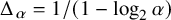 $\Delta _{\alpha } = 1/(1-\log _2 \alpha )$
when
$\Delta _{\alpha } = 1/(1-\log _2 \alpha )$
when
 $\alpha \in (1,2)$
. This coincides with our upper bound in Theorem 1.4 if
$\alpha \in (1,2)$
. This coincides with our upper bound in Theorem 1.4 if
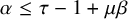 $\alpha \le \tau -1+\mu \beta $
. The same type of paths are used in both cases, passing through only low-degree vertices (and typical edge-costs on them for 1-FPP). For SFP, Lakis et al. prove in [Reference Lakis, Lengler, Petrova and Schiller60, Theorem 1.1] that graph distances and transmission times in Markovian FPP are also polylogarithmic when
$\alpha \le \tau -1+\mu \beta $
. The same type of paths are used in both cases, passing through only low-degree vertices (and typical edge-costs on them for 1-FPP). For SFP, Lakis et al. prove in [Reference Lakis, Lengler, Petrova and Schiller60, Theorem 1.1] that graph distances and transmission times in Markovian FPP are also polylogarithmic when
 $\alpha \in (1,2)$
and additionally
$\alpha \in (1,2)$
and additionally
 $\tau>3$
, with exponent
$\tau>3$
, with exponent
 $\Delta _G\in [1/(1-\log _2(\min (\alpha , \tau -2))),\Delta _{\alpha }]$
for graph distances and
$\Delta _G\in [1/(1-\log _2(\min (\alpha , \tau -2))),\Delta _{\alpha }]$
for graph distances and
 $\Delta _{\mathrm {FPP}}\in [1/(1-\log _2(\min (\alpha , (\tau -1)/2))), \Delta _\alpha ]$
for FPP, which improves earlier bounds [Reference Hao and Heydenreich46]. The lower-bound methods in [Reference Biskup and Lin12, Reference Trapman74, Reference Lakis, Lengler, Petrova and Schiller60] do not transfer to 1-FPP when
$\Delta _{\mathrm {FPP}}\in [1/(1-\log _2(\min (\alpha , (\tau -1)/2))), \Delta _\alpha ]$
for FPP, which improves earlier bounds [Reference Hao and Heydenreich46]. The lower-bound methods in [Reference Biskup and Lin12, Reference Trapman74, Reference Lakis, Lengler, Petrova and Schiller60] do not transfer to 1-FPP when
 $\tau \in (2,3)$
since they crucially rely on finite degree-variance
$\tau \in (2,3)$
since they crucially rely on finite degree-variance
 $\tau>3$
.
$\tau>3$
.
The linear phase. Linear distances are common in supercritical spatial graph models with bounded edge-lengths. For example, Random Geometric Graphs exhibit linear distances [Reference Penrose68], and so does supercritical percolation on grids of dimension at least
 $2$
[Reference Antal and Pisztora4]. Assuming high enough edge-density, a renormalisation argument to percolation on
$2$
[Reference Antal and Pisztora4]. Assuming high enough edge-density, a renormalisation argument to percolation on
 $\mathbb {Z}^d$
gives that SFP and LRP for
$\mathbb {Z}^d$
gives that SFP and LRP for
 $\tau>3$
and
$\tau>3$
and
 $\alpha>2$
also have at most linear graph-distances for
$\alpha>2$
also have at most linear graph-distances for
 $d\geq 2$
. The corresponding lower bound was shown by Berger for LRP [Reference Berger8] and by Deprez et al. for SFP [Reference Deprez, Hazra and Wüthrich27]. Our lower bound for 1-FPP contains these as special cases, and holds universally for classical FPP for any positive edge-transmission time-distribution [Reference Komjáthy, Lapinskas, Lengler and Schaller56, Corollary 1.12].
$d\geq 2$
. The corresponding lower bound was shown by Berger for LRP [Reference Berger8] and by Deprez et al. for SFP [Reference Deprez, Hazra and Wüthrich27]. Our lower bound for 1-FPP contains these as special cases, and holds universally for classical FPP for any positive edge-transmission time-distribution [Reference Komjáthy, Lapinskas, Lengler and Schaller56, Corollary 1.12].
The strictly polynomial phase. The phase where intrinsic distances scale as
 $|x-y|^{\eta _0+o(1)}$
with
$|x-y|^{\eta _0+o(1)}$
with
 $\eta _0<1$
(the result of Theorem 1.6) is quite rare in spatial settings and we only know two examples. One is in LRP at a boundary line in the parameter space, when
$\eta _0<1$
(the result of Theorem 1.6) is quite rare in spatial settings and we only know two examples. One is in LRP at a boundary line in the parameter space, when
 $\alpha =2$
[Reference Bäumler5, Reference Coppersmith, Gamarnik and Sviridenko24]. Our methods do not carry through for
$\alpha =2$
[Reference Bäumler5, Reference Coppersmith, Gamarnik and Sviridenko24]. Our methods do not carry through for
 $\alpha =2$
. The method in [Reference Bäumler5] for this setting uses the self-similarity of the model when
$\alpha =2$
. The method in [Reference Bäumler5] for this setting uses the self-similarity of the model when
 $\alpha =2$
and shows the sub-multiplicative structure of graph distances to obtain polynomial lower bounds. The other example is for long-range first passage percolation (LR-FPP) in [Reference Chatterjee and Dey20], mentioned at the beginning of this section. There are some similarities to 1-FPP: LR-FPP is Markovian, that is,
$\alpha =2$
and shows the sub-multiplicative structure of graph distances to obtain polynomial lower bounds. The other example is for long-range first passage percolation (LR-FPP) in [Reference Chatterjee and Dey20], mentioned at the beginning of this section. There are some similarities to 1-FPP: LR-FPP is Markovian, that is,
 $\beta =1$
in (1.3), and has strictly polynomial growth when
$\beta =1$
in (1.3), and has strictly polynomial growth when
 $\alpha '\in (2,2+1/d)$
, see Table 3. Using exponential L in 1-FPP, the length of the parameter interval
$\alpha '\in (2,2+1/d)$
, see Table 3. Using exponential L in 1-FPP, the length of the parameter interval
 $(\mu _{\log }, \mu _{\mathrm {pol}})$
with polynomial growth is also exactly
$(\mu _{\log }, \mu _{\mathrm {pol}})$
with polynomial growth is also exactly
 $1/d$
for
$1/d$
for
 $\mu $
when
$\mu $
when
 $\alpha>2+1/d$
, but it is longer when
$\alpha>2+1/d$
, but it is longer when
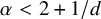 $\alpha <2+1/d$
, which shows that the penalty
$\alpha <2+1/d$
, which shows that the penalty
 $\alpha '$
of LR-FPP plays a slightly different role as the long-range parameter
$\alpha '$
of LR-FPP plays a slightly different role as the long-range parameter
 $\alpha $
in (1.5) here.
$\alpha $
in (1.5) here.
Gaps at approaching the phase boundaries. Here we discuss what happens as the parameters
 $\tau , \alpha , \mu , \beta $
approach the phase boundaries of growth. Some of these are indicated on Figure 3 by bold lines.
$\tau , \alpha , \mu , \beta $
approach the phase boundaries of growth. Some of these are indicated on Figure 3 by bold lines.
Polylogarithmic distances with exponent
 $\Delta _0$
heuristically imply stretched exponential ball-growth, where the number of vertices within intrinsic distance r scales as
$\Delta _0$
heuristically imply stretched exponential ball-growth, where the number of vertices within intrinsic distance r scales as
 $\exp (r^{1/\Delta _0})$
. Our upper bound exponent
$\exp (r^{1/\Delta _0})$
. Our upper bound exponent
 $\Delta _0=\min \{\Delta _\alpha , \Delta _\beta \}$
in (1.9) approaches
$\Delta _0=\min \{\Delta _\alpha , \Delta _\beta \}$
in (1.9) approaches
 $1$
as
$1$
as
 $\alpha \downarrow 1$
, and so does the exponent
$\alpha \downarrow 1$
, and so does the exponent
 $\Delta _{\alpha }$
of LRP [Reference Biskup11], which also partly governs SFP. This means that as
$\Delta _{\alpha }$
of LRP [Reference Biskup11], which also partly governs SFP. This means that as
 $\alpha \downarrow 1$
we approach exponential growth. In LRP, strictly exponential ball growth occurs only when
$\alpha \downarrow 1$
we approach exponential growth. In LRP, strictly exponential ball growth occurs only when
 $\alpha =1$
and the connectivity function has a suitably chosen slowly varying correction term
$\alpha =1$
and the connectivity function has a suitably chosen slowly varying correction term
 $\ell (\cdot )$
, that is,
$\ell (\cdot )$
, that is,
 $p(x,y)= \ell (|x-y|)/|x-y|^{\alpha d}$
, see [Reference Trapman74]. Strictly exponential growth is a natural barrier, since (age-dependent) branching processes with finite first moments exhibit at most exponential growth, and non-Markovian FPP can be dominated by such branching processes. Interestingly, when
$p(x,y)= \ell (|x-y|)/|x-y|^{\alpha d}$
, see [Reference Trapman74]. Strictly exponential growth is a natural barrier, since (age-dependent) branching processes with finite first moments exhibit at most exponential growth, and non-Markovian FPP can be dominated by such branching processes. Interestingly, when
 $\alpha>2$
and we approach the explosion phase transition by letting
$\alpha>2$
and we approach the explosion phase transition by letting
 $\mu \downarrow \mu _{\mathrm {expl}}=(3-\tau )/(2\beta )$
, then
$\mu \downarrow \mu _{\mathrm {expl}}=(3-\tau )/(2\beta )$
, then
 $\Delta _0$
in (1.9) does not converge to
$\Delta _0$
in (1.9) does not converge to
 $1$
, but to
$1$
, but to
 $1/(2-\log _2(\tau +1))=:\Delta _{\tau }$
. So, for the whole range
$1/(2-\log _2(\tau +1))=:\Delta _{\tau }$
. So, for the whole range
 $\tau \in (2,3)$
,
$\tau \in (2,3)$
,
 $\Delta _{\tau }\ge 1/(2-\log _2(3))> 2.4 > 1$
. As
$\Delta _{\tau }\ge 1/(2-\log _2(3))> 2.4 > 1$
. As
 $\tau \uparrow 3$
,
$\tau \uparrow 3$
,
 $\Delta _{\tau }$
approaches
$\Delta _{\tau }$
approaches
 $\infty $
, which is natural, since graph distances are linear already when
$\infty $
, which is natural, since graph distances are linear already when
 $\tau>3$
and
$\tau>3$
and
 $\alpha>2$
[Reference Deprez, Hazra and Wüthrich27]. This leaves two possibilities: our upper bound
$\alpha>2$
[Reference Deprez, Hazra and Wüthrich27]. This leaves two possibilities: our upper bound
 $\Delta _0$
is not sharp for
$\Delta _0$
is not sharp for
 $\alpha>2$
; or the ball growth jumps directly from subexponential (
$\alpha>2$
; or the ball growth jumps directly from subexponential (
 $\Delta _0>1$
) into the explosive phase. If the latter is the case, it would be interesting to understand better how such a jump could happen. Such jumps at phase boundaries may occur. This paper, together with [Reference Komjáthy, Lapinskas, Lengler and Schaller56], proves a gap in polynomial regime when
$\Delta _0>1$
) into the explosive phase. If the latter is the case, it would be interesting to understand better how such a jump could happen. Such jumps at phase boundaries may occur. This paper, together with [Reference Komjáthy, Lapinskas, Lengler and Schaller56], proves a gap in polynomial regime when
 $\tau $
crosses the threshold
$\tau $
crosses the threshold
 $3$
. The limits of
$3$
. The limits of
 $\lim _{\tau \uparrow 3}\mu _{\textrm {pol}}=1/d$
and
$\lim _{\tau \uparrow 3}\mu _{\textrm {pol}}=1/d$
and
 $\lim _{\tau \uparrow 3}\eta _0=\mu d$
exist and are in
$\lim _{\tau \uparrow 3}\eta _0=\mu d$
exist and are in
 $(0,1)$
in (1.8) and (1.10). So if we fix some
$(0,1)$
in (1.8) and (1.10). So if we fix some
 $\mu < 1/d$
and let
$\mu < 1/d$
and let
 $\tau \uparrow 3$
, the cost-distances grow polynomially with exponents bounded away from one (e.g., they approach
$\tau \uparrow 3$
, the cost-distances grow polynomially with exponents bounded away from one (e.g., they approach
 $1/2$
from below for
$1/2$
from below for
 $\mu = 1/(2d)$
). But as soon as
$\mu = 1/(2d)$
). But as soon as
 $\tau> 3$
is reached, the exponent ‘jumps’ to
$\tau> 3$
is reached, the exponent ‘jumps’ to
 $1$
and distances become strictly linear [Reference Komjáthy, Lapinskas, Lengler and Schaller56, Theorem 1.11]. So the parameter space is discontinuous in
$1$
and distances become strictly linear [Reference Komjáthy, Lapinskas, Lengler and Schaller56, Theorem 1.11]. So the parameter space is discontinuous in
 $\eta _0$
and
$\eta _0$
and
 $\mu _{\textrm {pol}}$
with respect to
$\mu _{\textrm {pol}}$
with respect to
 $\tau $
.
$\tau $
.
Some important questions are centred around such gaps. The gap conjecture in geometric group theory is about the ball growth of finitely generated groups: it states that there are no groups with growth between polynomial and stretched exponential of order
 $\exp (\Theta (\sqrt {n}))$
[Reference Grigorchuk43]. Although the polynomial side is understood by Gromov’s theorem [Reference Gromov44], the conjecture remains open. We find it intriguing to discover a deeper connection between phases of intrinsic growth in spatial random graphs (‘stochastic lattices’) and group theory (‘deterministic lattices’).
$\exp (\Theta (\sqrt {n}))$
[Reference Grigorchuk43]. Although the polynomial side is understood by Gromov’s theorem [Reference Gromov44], the conjecture remains open. We find it intriguing to discover a deeper connection between phases of intrinsic growth in spatial random graphs (‘stochastic lattices’) and group theory (‘deterministic lattices’).
Organisation. We start by moving to the quenched setting. In Section 2 we develop the nets, and in Section 3 the multiround exposure of edges, with the main result in Proposition 3.9. In Section 4 we collect some connectivity-estimates that serve as our building blocks, while in Section 5 we carry out the ‘budget travel plan’ and build a hierarchical path that only uses vertices of the net and connects vertices
 $y_0^\star , y_x^\star $
very close to
$y_0^\star , y_x^\star $
very close to
 $0$
and x, respectively. In Section 6 we connect
$0$
and x, respectively. In Section 6 we connect
 $0,x$
to these vertices with low cost, which is a nontrivial task itself, and prove the main theorems.
$0,x$
to these vertices with low cost, which is a nontrivial task itself, and prove the main theorems.
1.4.1 Notation
Throughout, we consider simple and undirected graphs with vertex set
 $\mathcal {V} \subseteq \mathbb {R}^d$
. For a graph
$\mathcal {V} \subseteq \mathbb {R}^d$
. For a graph
 $G=(\mathcal {V},\mathcal {E})$
and a set
$G=(\mathcal {V},\mathcal {E})$
and a set
 $A\subseteq \mathbb {R}^d$
,
$A\subseteq \mathbb {R}^d$
,
 $G[A]$
stands for the induced subgraph of G with vertex set
$G[A]$
stands for the induced subgraph of G with vertex set
 $\mathcal {V} \cap A$
. For two vertices
$\mathcal {V} \cap A$
. For two vertices
 $x,y\in \mathcal {V}$
, we denote the edge between them by
$x,y\in \mathcal {V}$
, we denote the edge between them by
 $xy$
, and for a set
$xy$
, and for a set
 $V\subseteq \mathcal {V}$
we write
$V\subseteq \mathcal {V}$
we write
 $V^{(2)} := \{\{x,y\} : x,y\in V, x\neq y\}$
for the set of possible edges among vertices in V. For a path
$V^{(2)} := \{\{x,y\} : x,y\in V, x\neq y\}$
for the set of possible edges among vertices in V. For a path
 $\pi $
,
$\pi $
,
 $\mathcal {E}(\pi )$
is the set of edges forming
$\mathcal {E}(\pi )$
is the set of edges forming
 $\pi $
, and
$\pi $
, and
 $|\pi |$
is the number of edges of
$|\pi |$
is the number of edges of
 $\pi $
. Generally the size of a discrete set S is
$\pi $
. Generally the size of a discrete set S is
 $|S|$
, while of a set
$|S|$
, while of a set
 $A\subseteq \mathbb {R}^d$
,
$A\subseteq \mathbb {R}^d$
,
 $\mathrm {Vol}(A)$
is its Lebesgue measure. Given a cost function
$\mathrm {Vol}(A)$
is its Lebesgue measure. Given a cost function
 $\mathcal {C}: \mathcal {E} \to [0,\infty ]$
on the edges, the cost of a set of edges
$\mathcal {C}: \mathcal {E} \to [0,\infty ]$
on the edges, the cost of a set of edges
 $\mathcal {P}$
is
$\mathcal {P}$
is
 $\mathcal {C}(\mathcal {P}):=\sum _{e\in \mathcal {E}(\mathcal {P})}\mathcal {C}(e)$
. We define
$\mathcal {C}(\mathcal {P}):=\sum _{e\in \mathcal {E}(\mathcal {P})}\mathcal {C}(e)$
. We define
 $\mathcal {C}(xx):=0$
for all
$\mathcal {C}(xx):=0$
for all
 $x\in \mathcal {V}$
. We define the cost-distance between vertices x and y as
$x\in \mathcal {V}$
. We define the cost-distance between vertices x and y as
 $$ \begin{align} d_{\mathcal{C}}(x,y):=\inf\{\mathcal{C}(\pi) : \pi \text{ is a path from } x \text{ to } y \text{ in } G\}. \end{align} $$
We define the graph distance
 $d_G(x,y)$
similarly, where all edge-costs are set to
$d_G(x,y)$
similarly, where all edge-costs are set to
 $1$
. We denote the Euclidean norm of
$1$
. We denote the Euclidean norm of
 $x \in \mathbb R^d$
by
$x \in \mathbb R^d$
by
 $|x|$
, the Euclidean ball with radius
$|x|$
, the Euclidean ball with radius
 $r\geq 0$
around x by
$r\geq 0$
around x by
 $B_r(x) := \{y\in \mathbb {R}^d : |x-y|\le r\}$
, and the set of vertices in this ball by
$B_r(x) := \{y\in \mathbb {R}^d : |x-y|\le r\}$
, and the set of vertices in this ball by
 $\mathcal {B}_r(x):=\{y\in \mathcal {V} : |x-y|\le r\} = B_r(x) \cap \mathcal {V}$
. (The minimal notation difference is intentional). The graph-distance ball and cost-distance ball (or cost-ball for short) around a vertex x are the vertex sets
$\mathcal {B}_r(x):=\{y\in \mathcal {V} : |x-y|\le r\} = B_r(x) \cap \mathcal {V}$
. (The minimal notation difference is intentional). The graph-distance ball and cost-distance ball (or cost-ball for short) around a vertex x are the vertex sets
 $\mathcal {B}_r^G(x):=\{y\in \mathcal {V} : d_G(x,y)\le r\}$
and
$\mathcal {B}_r^G(x):=\{y\in \mathcal {V} : d_G(x,y)\le r\}$
and
 $\mathcal {B}_r^{\mathcal {C}}(x):=\{y\in \mathcal {V} : d_{\mathcal {C}}(x,y)\le r\}$
, respectively. We set
$\mathcal {B}_r^{\mathcal {C}}(x):=\{y\in \mathcal {V} : d_{\mathcal {C}}(x,y)\le r\}$
, respectively. We set
 $B_r := B_r(0)$
, and do similarly for
$B_r := B_r(0)$
, and do similarly for
 $\mathcal {B}_r$
,
$\mathcal {B}_r$
,
 $\mathcal {B}_r^G$
,
$\mathcal {B}_r^G$
,
 $\mathcal {B}_r^{\mathcal {C}}$
if
$\mathcal {B}_r^{\mathcal {C}}$
if
 $0$
is a vertex. We define
$0$
is a vertex. We define
 $\partial B_r(x) := B_r(x)\setminus \{y\in \mathbb {R}^d : |x-y| < r\}$
, and use similar definitions for
$\partial B_r(x) := B_r(x)\setminus \{y\in \mathbb {R}^d : |x-y| < r\}$
, and use similar definitions for
 $\partial \mathcal {B}_r$
,
$\partial \mathcal {B}_r$
,
 $\partial \mathcal {B}_r^G$
and
$\partial \mathcal {B}_r^G$
and
 $\partial \mathcal {B}_r^{\mathcal {C}}$
. In particular,
$\partial \mathcal {B}_r^{\mathcal {C}}$
. In particular,
 $\partial \mathcal {B}_1^G(v)$
is the set of neighbours of v.
$\partial \mathcal {B}_1^G(v)$
is the set of neighbours of v.
The set of model parameters are
 $ {\texttt {par}} := \{d, \tau , \alpha , \mu , \beta , \underline {c}, \overline {c}, c_1, c_2, t_0\}$
. For parameters
$ {\texttt {par}} := \{d, \tau , \alpha , \mu , \beta , \underline {c}, \overline {c}, c_1, c_2, t_0\}$
. For parameters
 $a,b>0$
(model parameters or otherwise), we use ‘for all
$a,b>0$
(model parameters or otherwise), we use ‘for all
 $a{\,\gg _{\star }\,} b$
’ as shortcut for ‘
$a{\,\gg _{\star }\,} b$
’ as shortcut for ‘
 $\forall b>0:\, \exists a_0 = a_0(b):\, \forall a\ge a_0$
’. We also say ‘
$\forall b>0:\, \exists a_0 = a_0(b):\, \forall a\ge a_0$
’. We also say ‘
 $a {\,\gg _{\star }\,} b$
’ to mean that
$a {\,\gg _{\star }\,} b$
’ to mean that
 $a \ge a_0(b)$
. We use
$a \ge a_0(b)$
. We use
 $a {\,\ll _{\star }\,} b$
analogously, and may use more than two parameters. For example, ‘for
$a {\,\ll _{\star }\,} b$
analogously, and may use more than two parameters. For example, ‘for
 $a{\,\gg _{\star }\,} b,c$
’ means ‘
$a{\,\gg _{\star }\,} b,c$
’ means ‘
 $\forall b,c>0:\, \exists a_0=a_0(b,c):\, \forall a \ge a_0$
’. A measurable function
$\forall b,c>0:\, \exists a_0=a_0(b,c):\, \forall a \ge a_0$
’. A measurable function
 $\ell :(0,\infty ) \to (0,\infty )$
is said to be slowly varying at infinity if
$\ell :(0,\infty ) \to (0,\infty )$
is said to be slowly varying at infinity if
 $\lim _{x\to \infty } \ell (cx)/\ell (x) =1$
for all
$\lim _{x\to \infty } \ell (cx)/\ell (x) =1$
for all
 $c>0$
. We denote by
$c>0$
. We denote by
 $\log $
the natural logarithm, by
$\log $
the natural logarithm, by
 $\log _2$
the logarithm with base
$\log _2$
the logarithm with base
 $2$
, and by
$2$
, and by
 $\log ^{*k}$
the k-fold iterated logarithm, for example,
$\log ^{*k}$
the k-fold iterated logarithm, for example,
 $\log ^{*3}x = \log \log \log x$
. For
$\log ^{*3}x = \log \log \log x$
. For
 $n \in \mathbb {N}$
we write
$n \in \mathbb {N}$
we write
 $[n]:= \{1,\ldots ,n\}$
, and for an event
$[n]:= \{1,\ldots ,n\}$
, and for an event
 $\mathcal {A}$
we denote by
$\mathcal {A}$
we denote by
 $\mathcal {A}^\complement $
its complement.
$\mathcal {A}^\complement $
its complement.
2 Working conditionally on the weighted vertex-set: nets
In proving the upper bounds (Theorems 1.4 and 1.6), we will construct cheap paths along the lines of the ‘budget travel plan’ on page 7 in Section 1, which is an iterative scheme of finding long 3-edge bridge-paths to connect two far-away vertices. Since low-cost events in 1-FPP are not increasing, we develop a technique that replaces the FKG-inequality. Moving to the quenched setting, we will first expose all vertex positions and weights (above some threshold weight, in the case of IGIRG); then, low-cost edge existence events become independent. To be able to work with fixed realisations of the vertex set, we find (with high probability as
 $|x|\to \infty $
) a ‘nice’ subset of the vertices, that is, that behaves regularly enough inside a box around
$|x|\to \infty $
) a ‘nice’ subset of the vertices, that is, that behaves regularly enough inside a box around
 $0,x$
, as in (1.4), which we call a net. We formalise the notion of the nets now. We start with a less demanding notion of nets that we call weak nets which will suffice for the further sections of the paper. Their existence will follow from the existence of strong nets which make (1.4) precise; this may be of independent interest, and most of the section shall be devoted to proving their existence.
$0,x$
, as in (1.4), which we call a net. We formalise the notion of the nets now. We start with a less demanding notion of nets that we call weak nets which will suffice for the further sections of the paper. Their existence will follow from the existence of strong nets which make (1.4) precise; this may be of independent interest, and most of the section shall be devoted to proving their existence.
The vertex-weight distribution satisfies
 $\mathbb {P}(W\ge w)=\ell (w)w^{-(\tau -1)}$
in Definition 1.3, and consider the slowly varying function
$\mathbb {P}(W\ge w)=\ell (w)w^{-(\tau -1)}$
in Definition 1.3, and consider the slowly varying function
 $\ell (w)$
from (1.6). We define
$\ell (w)$
from (1.6). We define
 $w_0$
to be the smallest integer in
$w_0$
to be the smallest integer in
 $[1,\infty )$
such that
$[1,\infty )$
such that
 $$ \begin{align} \forall w>w_0, \forall t \in [1/2, 2]: \quad \ell(w)w^{-(\tau-1)} < 2^{-\tau-8} \quad \text{and}\quad 0.99 \le \ell(t w)/\ell(w) \le 1.01 \end{align} $$
both hold. Note that
 $w_0$
satisfying (2.1) must exist since
$w_0$
satisfying (2.1) must exist since
 $\ell $
is a slowly varying function, and so Potter’s bound [Reference Bingham, Goldie and Teugels10] ensures the first inequality.
$\ell $
is a slowly varying function, and so Potter’s bound [Reference Bingham, Goldie and Teugels10] ensures the first inequality.
For a set
 $A\subset \mathbb {R}^d$
we write
$A\subset \mathbb {R}^d$
we write
 $\mathrm {Vol}(A)$
for its Lebesgue measure (volume), while for a discrete set
$\mathrm {Vol}(A)$
for its Lebesgue measure (volume), while for a discrete set
 $\mathcal {A}\subseteq (0,\infty )$
we write
$\mathcal {A}\subseteq (0,\infty )$
we write
 $|\mathcal {A}|$
for the cardinality (size) of the set. Recall that weighted vertices are of the form
$|\mathcal {A}|$
for the cardinality (size) of the set. Recall that weighted vertices are of the form
 $\tilde v=(v, w_v)\in \mathbb {R}^d\times [1,\infty )$
.
$\tilde v=(v, w_v)\in \mathbb {R}^d\times [1,\infty )$
.
Definition 2.1 (Weak net).
Let
 $Q \subseteq \mathbb {R}^d$
be a box of side length
$Q \subseteq \mathbb {R}^d$
be a box of side length
 $\xi $
,
$\xi $
,
 $\varepsilon>0$
, and
$\varepsilon>0$
, and
 $w_1 \geq w_0$
. A weak
$w_1 \geq w_0$
. A weak
 $(\varepsilon ,w_1)$
-net for Q is a set
$(\varepsilon ,w_1)$
-net for Q is a set
 $\mathcal {N} \subseteq \widetilde {\mathcal {V}} \cap Q\times [1,\infty )$
of size at least
$\mathcal {N} \subseteq \widetilde {\mathcal {V}} \cap Q\times [1,\infty )$
of size at least
 $\mathrm {Vol}(Q)/4$
such that for all
$\mathrm {Vol}(Q)/4$
such that for all
 $\widetilde {v} \in \mathcal {N}$
, all
$\widetilde {v} \in \mathcal {N}$
, all
 $r \in [(\log \log \xi \sqrt {d})^{4/\varepsilon }, \xi \sqrt {d}]$
and all
$r \in [(\log \log \xi \sqrt {d})^{4/\varepsilon }, \xi \sqrt {d}]$
and all
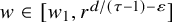 $w \in [w_1, r^{d/(\tau -1)-\varepsilon }]$
:
$w \in [w_1, r^{d/(\tau -1)-\varepsilon }]$
:
 $$ \begin{align} |\mathcal{N}\cap (B_r(v)\times [w/2, 2w])| \ge r^{d(1-\varepsilon)}\cdot \ell(w)w^{-(\tau-1)}. \end{align} $$
In a weak
 $(\varepsilon ,w_1)$
-net, the number of weighted vertices in balls around net-vertices are close to their expectation. Since we only require the property to hold around net vertices and not everywhere, we circumvent the issue that the vertex set may have empty/low-density areas. In a weak net, we allow an error of order
$(\varepsilon ,w_1)$
-net, the number of weighted vertices in balls around net-vertices are close to their expectation. Since we only require the property to hold around net vertices and not everywhere, we circumvent the issue that the vertex set may have empty/low-density areas. In a weak net, we allow an error of order
 $r^{-d\varepsilon }$
on the right-hand side of (2.2), and the minimal radius of the balls around net vertices grows with the size
$r^{-d\varepsilon }$
on the right-hand side of (2.2), and the minimal radius of the balls around net vertices grows with the size
 $\xi $
of the box Q. In a strong net, we shall only allow a constant factor loss, see (2.4), and the balls can have constant radii r. The result that we shall use in further sections is the following, again using the Palm measure in the case of IGIRG [Reference Last and Penrose61]. We condition on a few vertices to be part of the vertex set and also demand that these vertices are part of the net.
$\xi $
of the box Q. In a strong net, we shall only allow a constant factor loss, see (2.4), and the balls can have constant radii r. The result that we shall use in further sections is the following, again using the Palm measure in the case of IGIRG [Reference Last and Penrose61]. We condition on a few vertices to be part of the vertex set and also demand that these vertices are part of the net.
Lemma 2.2. Consider IGIRG or SFP with
 $\tau \!>\!2$
in Def. 1.3. Then for all
$\tau \!>\!2$
in Def. 1.3. Then for all
 $\varepsilon \in (0,1/2)$
, and for all
$\varepsilon \in (0,1/2)$
, and for all
 $\xi $
sufficiently large relative to
$\xi $
sufficiently large relative to
 $\varepsilon $
, and
$\varepsilon $
, and
 $t \le \min \{1/\varepsilon ,\log \log \xi \}$
the following holds. Consider a cube
$t \le \min \{1/\varepsilon ,\log \log \xi \}$
the following holds. Consider a cube
 $Q \subseteq \mathbb {R}^d$
of side length
$Q \subseteq \mathbb {R}^d$
of side length
 $\xi $
, and let
$\xi $
, and let
 $x_1,\ldots ,x_t \in Q$
, and
$x_1,\ldots ,x_t \in Q$
, and
 $w_0$
from (2.1), then
$w_0$
from (2.1), then
 $$ \begin{align*} \mathbb{P}(Q \text{ contains a weak } (\varepsilon,w_0)\text{-net } \mathcal{N}, \text{ and } x_1,\ldots,x_t \in \mathcal{N} \mid x_1,\ldots,x_t \in \mathcal{V} ) \ge 1-t\varepsilon. \end{align*} $$
The condition
 $t\le 1/\varepsilon $
is there to avoid a vacuous statement, and below we set
$t\le 1/\varepsilon $
is there to avoid a vacuous statement, and below we set
 $t=2$
and replace the conditioning by
$t=2$
and replace the conditioning by
 $0,x\in \mathcal {V}$
. Note that the condition (2.2) never counts vertices of weight less than
$0,x\in \mathcal {V}$
. Note that the condition (2.2) never counts vertices of weight less than
 $w_1/2$
. So, we can decide whether a weak
$w_1/2$
. So, we can decide whether a weak
 $(\varepsilon ,w_1)$
-net
$(\varepsilon ,w_1)$
-net
 $\mathcal {N}$
exists by uncovering only the set of vertices of weight at least
$\mathcal {N}$
exists by uncovering only the set of vertices of weight at least
 $w_1/2$
(beyond
$w_1/2$
(beyond
 $x_1,\ldots ,x_t \in \mathcal {N}$
). For IGIRG, this set is independent of the set of vertices of weight smaller than
$x_1,\ldots ,x_t \in \mathcal {N}$
). For IGIRG, this set is independent of the set of vertices of weight smaller than
 $w_1/2$
, and we may use low-weight vertices for other purposes. This is the main reason for introducing the parameter
$w_1/2$
, and we may use low-weight vertices for other purposes. This is the main reason for introducing the parameter
 $w_1$
. We mention that Q does not need be a box of equal sizes, the proof also works for boxes of any finite proportions parametrised by constant multiples of
$w_1$
. We mention that Q does not need be a box of equal sizes, the proof also works for boxes of any finite proportions parametrised by constant multiples of
 $\xi $
.
$\xi $
.
In order to prove the existence of weak nets, we will divide Q into nested sub-boxes and work inductively, taking the finest partition and lowest-weight vertices as the base case and gradually coarsening the partition and including higher-weight vertices. To make this argument work, we will need stronger control over the properties of each layer of the partition than Definition 2.1 provides; see Definition 2.10. As such, it is convenient to instead prove the existence of ‘strong nets’ which satisfy tighter bounds at specific scales, which we define next. We will then prove that every strong net is also a weak net, as our strong control at each layer will translate into weaker control between layers. Strong nets may also be of independent interest in cases where stronger bounds over smaller scales are required.
Recall
 $w_0$
from (2.1). For all
$w_0$
from (2.1). For all
 $\delta>0$
, and
$\delta>0$
, and
 $R>0$
we define the function
$R>0$
we define the function
 $f_{R,\delta }(r)$
slightly below the typical largest vertex weight in a ball of radius r (roughly
$f_{R,\delta }(r)$
slightly below the typical largest vertex weight in a ball of radius r (roughly
 $r^{d/(\tau -1)}$
):
$r^{d/(\tau -1)}$
):
 $$ \begin{align} f_{R,\delta}(r) = r^{\frac{d}{\tau-1}} \left(1 \wedge \inf\big\{\ell(x)\colon x \in [w_0,r^{d/(\tau-1)}]\big\}\right)^{\frac{1}{\tau-1}}\cdot \left(\frac{1}{(2d)^{2\tau+d+8}\log(16 R/\delta)}\right)^{\frac{1}{\tau-1}}. \end{align} $$
Definition 2.3 (Strong net).
Let
 $G=(\mathcal {V},\mathcal {E})$
be an IGIRG or SFP as in Definition 1.3. Let
$G=(\mathcal {V},\mathcal {E})$
be an IGIRG or SFP as in Definition 1.3. Let
 $\mathcal {R}=(r_1, r_2, \dots , r_R) \subseteq (0,\infty )$
be an increasing list of radii with
$\mathcal {R}=(r_1, r_2, \dots , r_R) \subseteq (0,\infty )$
be an increasing list of radii with
 $R=|\mathcal {R}|<\infty $
, let
$R=|\mathcal {R}|<\infty $
, let
 $w_0$
be as in (2.1) and
$w_0$
be as in (2.1) and
 $f_{R,\delta }(\cdot )$
be as in (2.3). Let
$f_{R,\delta }(\cdot )$
be as in (2.3). Let
 $Q \subseteq \mathbb {R}^d$
be a box. A
$Q \subseteq \mathbb {R}^d$
be a box. A
 $(\delta ,\mathcal {R})$
-net for Q is a set
$(\delta ,\mathcal {R})$
-net for Q is a set
 $\mathcal {N} \subseteq \widetilde {\mathcal {V}} \cap Q\times [1,\infty )$
of size at least
$\mathcal {N} \subseteq \widetilde {\mathcal {V}} \cap Q\times [1,\infty )$
of size at least
 $\mathrm {Vol}(Q)/4$
such that for all
$\mathrm {Vol}(Q)/4$
such that for all
 $\tilde v \in \mathcal {N}$
,
$\tilde v \in \mathcal {N}$
,
 $r \in \mathcal {R}$
, and all
$r \in \mathcal {R}$
, and all
 $w \in [w_0,f_{R,\delta }(r)]$
,
$w \in [w_0,f_{R,\delta }(r)]$
,
 $$ \begin{align} \left| \big\{\widetilde u\in \mathcal{N}\cap B_r(v) \times [w/2, 2w] \big\}\right| \ge r^d\cdot \ell(w)w^{-(\tau-1)}/(2d)^{d+\tau+5}. \end{align} $$
Each
 $r \in \mathcal {R}$
in Definition 2.3 will correspond to a layer of the discretisation of Q alluded to above. We will require these radii to grow at least exponentially, with base depending on the number R of radii in the list. The specific condition is the following. It may seem very strong that we require (2.4) for infinitely many w. We discretise
$r \in \mathcal {R}$
in Definition 2.3 will correspond to a layer of the discretisation of Q alluded to above. We will require these radii to grow at least exponentially, with base depending on the number R of radii in the list. The specific condition is the following. It may seem very strong that we require (2.4) for infinitely many w. We discretise
 $[w_0, f_{R,\delta }(r)]$
into a finite set of subintervals
$[w_0, f_{R,\delta }(r)]$
into a finite set of subintervals
 $(I_j)_{j\le j_{\max }}$
in a smart way. Then we ensure that (2.4) holds with
$(I_j)_{j\le j_{\max }}$
in a smart way. Then we ensure that (2.4) holds with
 $[w/2, 2w]$
replaced by
$[w/2, 2w]$
replaced by
 $I_j$
on the left hand side and the
$I_j$
on the left hand side and the
 $\ell (w)w^{-(\tau -1)}$
replaced by
$\ell (w)w^{-(\tau -1)}$
replaced by
 $\mathbb P(W\in I_j)$
on the right hand side, and then this will imply that (2.4) also holds for all values
$\mathbb P(W\in I_j)$
on the right hand side, and then this will imply that (2.4) also holds for all values
 $w\in [w_0, f_{R,\delta }(r)]$
.
$w\in [w_0, f_{R,\delta }(r)]$
.
Definition 2.4. Fix
 $\delta \in (0,1)$
. We say that an increasing list of radii
$\delta \in (0,1)$
. We say that an increasing list of radii
 $\mathcal {R}=(r_1, r_2, \dots , r_R) \subseteq (0,\infty )$
is
$\mathcal {R}=(r_1, r_2, \dots , r_R) \subseteq (0,\infty )$
is
 $\delta $
-well-spaced if
$\delta $
-well-spaced if
 $R=|\mathcal {R}|<\infty $
and the following hold:
$R=|\mathcal {R}|<\infty $
and the following hold:
 $$ \begin{align} r_1 &\ge 24d\big(\log(4R/\delta)\big)^{1/d} \vee w_0^{(\tau-1)/d} \vee \inf\{r \colon f_{R,\delta}(r) \ge w_0\}; \end{align} $$
 $$ \begin{align}\frac{r_i}{r_{i-1}} &\ge 6R^{1/d}\left(\frac{\log(2R/\delta)}{\delta}\right)^{1/d} \quad \forall i\in [2,R]. \end{align} $$
In Definition 2.3, it may seem very strong that we require (2.4) for infinitely many w. We discretise
 $[w_0, f_{R,\delta }(r)]$
into a finite set of subintervals
$[w_0, f_{R,\delta }(r)]$
into a finite set of subintervals
 $(I_j)_{j\le j_{\max }}$
in a smart way. Then we ensure that (2.4) holds with
$(I_j)_{j\le j_{\max }}$
in a smart way. Then we ensure that (2.4) holds with
 $[w/2, 2w]$
replaced by
$[w/2, 2w]$
replaced by
 $I_j$
on the left hand side and the
$I_j$
on the left hand side and the
 $\ell (w)w^{-(\tau -1)}$
replaced by
$\ell (w)w^{-(\tau -1)}$
replaced by
 $\mathbb P(W\in I_j)$
on the right hand side, and then this will imply that (2.4) also holds for all values
$\mathbb P(W\in I_j)$
on the right hand side, and then this will imply that (2.4) also holds for all values
 $w\in [w_0, f_{R,\delta }(r)]$
.
$w\in [w_0, f_{R,\delta }(r)]$
.
We now state the main result of the section. Heuristically, a box Q contains an
 $(\delta ,\mathcal {R})$
-net with sufficiently high probability, and we can also condition on the presence of a few vertices in the net. The condition
$(\delta ,\mathcal {R})$
-net with sufficiently high probability, and we can also condition on the presence of a few vertices in the net. The condition
 $t\le 1/\delta $
in the following is added to avoid a vacuous statement.
$t\le 1/\delta $
in the following is added to avoid a vacuous statement.
Proposition 2.5. Consider IGIRG or SFP with
 $\tau> 2$
. Let
$\tau> 2$
. Let
 $\delta \in (0,1/16), \xi> 0$
, and
$\delta \in (0,1/16), \xi> 0$
, and
 $Q \subseteq \mathbb {R}^d$
be a cube of side length
$Q \subseteq \mathbb {R}^d$
be a cube of side length
 $\xi $
. Let
$\xi $
. Let
 $R\in \mathbb {N}$
and
$R\in \mathbb {N}$
and
 $\mathcal {R}=\{r_1, \ldots , r_R\}$
be a
$\mathcal {R}=\{r_1, \ldots , r_R\}$
be a
 $\delta $
-well-spaced increasing list of radii with
$\delta $
-well-spaced increasing list of radii with
 $r_R = \xi \sqrt {d}$
. Let
$r_R = \xi \sqrt {d}$
. Let
 $x_1,\ldots ,x_t \in Q$
with
$x_1,\ldots ,x_t \in Q$
with
 $t \le \min \{1/\delta ,(r_1/4\sqrt {d})^d\}$
, for SFP assume
$t \le \min \{1/\delta ,(r_1/4\sqrt {d})^d\}$
, for SFP assume
 $x_1, \ldots x_t \subset \mathbb {Z}^d$
also. Then
$x_1, \ldots x_t \subset \mathbb {Z}^d$
also. Then
$$ \begin{align} \mathbb{P}&(Q \text{ contains an } (\delta,\mathcal{R})\text{-net } \mathcal{N})\ge 1-\delta/R; \end{align} $$
 $$ \begin{align} \mathbb{P}&(Q \text{ contains an } (\delta,\mathcal{R})\text{-net } \mathcal{N}, x_1,\ldots,x_t \in \mathcal{N} \mid x_1,\ldots,x_t \in \mathcal{V} ) \ge 1-t\delta. \end{align} $$
For IGIRG (2.8) uses the Palm measure of vertex-weights and positions for IGIRG. For SFP the conditioning can be dropped.
The proof of this proposition will take the rest of the section. Before that we show how Lemma 2.2 follows from it.
Proof of Lemma 2.2 subject to Proposition 2.5.
Let
 $\varepsilon \in (0,1/2)$
, set
$\varepsilon \in (0,1/2)$
, set
 $\eta := 1 - \varepsilon /2$
, and define
$\eta := 1 - \varepsilon /2$
, and define
 $\mathcal {R} = \{r_1,\ldots ,r_R\}$
as
$\mathcal {R} = \{r_1,\ldots ,r_R\}$
as
 $$ \begin{align} R &:= 2 + \lfloor(\log\log\xi\sqrt{d} - \log^{*4}\xi\sqrt{d}-\log\tfrac{4}{\varepsilon})/\log(1/\eta)\rfloor, \end{align} $$
 $$ \begin{align} r_i &:= (\xi\sqrt{d})^{\eta^{R-i}}, \quad\text{for} \quad i\in[R]. \end{align} $$
We show that this choice of
 $\mathcal {R}$
is
$\mathcal {R}$
is
 $\varepsilon $
-well-spaced (Def. 2.4). Let
$\varepsilon $
-well-spaced (Def. 2.4). Let
 $1-a\in [0,1)$
be the fractional part of the expression inside the
$1-a\in [0,1)$
be the fractional part of the expression inside the
 $\lfloor \cdot \rfloor $
in (2.9). Then using that
$\lfloor \cdot \rfloor $
in (2.9). Then using that
 $\lfloor x\rfloor =x-1+a$
,
$\lfloor x\rfloor =x-1+a$
,
$$ \begin{align} r_1 = (\xi\sqrt{d})^{\eta^{R-1}} = (\xi\sqrt{d})^{\eta^{a}4\log^{*3}\xi\sqrt{d}/(\varepsilon\log\xi\sqrt{d})} = (\log\log\xi\sqrt{d})^{(1-\varepsilon/2)^{a}4/\varepsilon}. \end{align} $$
Since
 $a\in (0,1]$
and
$a\in (0,1]$
and
 $\varepsilon <1/2$
, this implies that
$\varepsilon <1/2$
, this implies that
 $r_1$
is a strictly larger power of
$r_1$
is a strictly larger power of
 $\log \log \xi \sqrt {d}$
than
$\log \log \xi \sqrt {d}$
than
 $1$
while R is of order
$1$
while R is of order
 $\log \log \xi \sqrt {d}$
. Since
$\log \log \xi \sqrt {d}$
. Since
 $\xi $
is large relative to
$\xi $
is large relative to
 $\varepsilon $
, Def. 2.4 (2.5) holds for
$\varepsilon $
, Def. 2.4 (2.5) holds for
 $\varepsilon =\delta $
. For all
$\varepsilon =\delta $
. For all
 $i \in [R]$
, since
$i \in [R]$
, since
 $\eta =1-\varepsilon /2$
:
$\eta =1-\varepsilon /2$
:
 $$\begin{align*}r_i/r_{i-1} = (\xi\sqrt{d})^{\eta^{R-i}(1-\eta)} \ge (\xi\sqrt{d})^{\eta^{R-1}\varepsilon/2} = r_1^{\varepsilon/2} = (\log\log\xi\sqrt{d})^{2(1-\varepsilon/2)^{a}}. \end{align*}$$
Since
 $a\le 1$
,
$a\le 1$
,
 $2(1-\varepsilon /2)^{a}>1$
for all
$2(1-\varepsilon /2)^{a}>1$
for all
 $\varepsilon <1/2$
, so Def. 2.4 (2.6) holds even in
$\varepsilon <1/2$
, so Def. 2.4 (2.6) holds even in
 $d=1$
, and
$d=1$
, and
 $\mathcal {R}$
is
$\mathcal {R}$
is
 $\varepsilon $
-well-spaced as claimed. Moreover, since
$\varepsilon $
-well-spaced as claimed. Moreover, since
 $t \le \log \log \xi $
by hypothesis, by (2.11) we have
$t \le \log \log \xi $
by hypothesis, by (2.11) we have
 $t \le (r_1/4\sqrt {d})^d$
. By Proposition 2.5, with probability at least
$t \le (r_1/4\sqrt {d})^d$
. By Proposition 2.5, with probability at least
 $1-t\varepsilon $
, conditioned on
$1-t\varepsilon $
, conditioned on
 $x_1,\ldots ,x_t\in \mathcal {V}$
, Q contains a strong
$x_1,\ldots ,x_t\in \mathcal {V}$
, Q contains a strong
 $(\varepsilon ,\mathcal {R})$
-net
$(\varepsilon ,\mathcal {R})$
-net
 $\mathcal {N}$
in Def. 2.3. We now show that a strong net is also a weak net (with the same
$\mathcal {N}$
in Def. 2.3. We now show that a strong net is also a weak net (with the same
 $\varepsilon )$
. Fix an arbitrary
$\varepsilon )$
. Fix an arbitrary
 $r \in [(\log \log \xi \sqrt {d})^{4/\varepsilon }, \xi \sqrt {d}]$
and
$r \in [(\log \log \xi \sqrt {d})^{4/\varepsilon }, \xi \sqrt {d}]$
and
 $w \in [w_0,r^{d/(\tau -1)-\varepsilon }]$
as in Def. 2.1 (this interval is nonempty since
$w \in [w_0,r^{d/(\tau -1)-\varepsilon }]$
as in Def. 2.1 (this interval is nonempty since
 $\tau \in (2,3), \varepsilon <1/2$
), and consider a vertex
$\tau \in (2,3), \varepsilon <1/2$
), and consider a vertex
 $v \in \mathcal {N}$
. Since
$v \in \mathcal {N}$
. Since
 $a>0$
in (2.11), we have
$a>0$
in (2.11), we have
 $r_1 \le r \le r_R$
. Let
$r_1 \le r \le r_R$
. Let
 $r_j$
be such that
$r_j$
be such that
 $r\in [r_j,r_{j+1})$
; thus
$r\in [r_j,r_{j+1})$
; thus
 $r^{\eta } \le r_j \le r$
by (2.10). Since
$r^{\eta } \le r_j \le r$
by (2.10). Since
 $\xi $
is large relative to
$\xi $
is large relative to
 $\varepsilon $
, we have
$\varepsilon $
, we have
 $w \le f_{R,\varepsilon }(r_j)$
(using (2.3)) for
$w \le f_{R,\varepsilon }(r_j)$
(using (2.3)) for
 $f_{R,\varepsilon }$
); thus by the definition of a strong
$f_{R,\varepsilon }$
); thus by the definition of a strong
 $(\varepsilon , \mathcal {R})$
-net in Def. 2.3,
$(\varepsilon , \mathcal {R})$
-net in Def. 2.3,
 $|\mathcal {N} \cap (B_{r_j}(v)\times [w/2, 2w])|\ge \ell (w)w^{-(\tau -1)}r_j^d/(2d)^{d+\tau +5}$
. Since
$|\mathcal {N} \cap (B_{r_j}(v)\times [w/2, 2w])|\ge \ell (w)w^{-(\tau -1)}r_j^d/(2d)^{d+\tau +5}$
. Since
 $\xi $
is large relative to
$\xi $
is large relative to
 $\varepsilon $
and
$\varepsilon $
and
 $r \ge r_j \ge r^{\eta }$
, the required inequality in Def. 2.1 follows since
$r \ge r_j \ge r^{\eta }$
, the required inequality in Def. 2.1 follows since
 $$\begin{align*}|\mathcal{N} \cap (B_{r}(v)\times[w/2, 2w])| \ge \ell(w)w^{-(\tau-1)}r^{d\eta}/(2d)^{d+\tau+5} \ge \ell(w)w^{-(\tau-1)}r^{d(1-\varepsilon)}. \end{align*}$$
The rest of this section is devoted to proving Proposition 2.5. All remaining definitions and lemmas are used only within this section.
Shortly we shall carry out a multiscale analysis. We abbreviate
 $f_{R,\delta }:=f$
everywhere except in definitions and statements. We partition
$f_{R,\delta }:=f$
everywhere except in definitions and statements. We partition
 $Q\times [w_0, f(r_R)]$
into hyper-rectangles. On the weight-coordinate, we cover the interval
$Q\times [w_0, f(r_R)]$
into hyper-rectangles. On the weight-coordinate, we cover the interval
 $[w_0,f(r_R)]$
of weights with a set of disjoint intervals
$[w_0,f(r_R)]$
of weights with a set of disjoint intervals
 $(I_j)_{j=1, \ldots , j_{\max }}$
so that the first interval is of length
$(I_j)_{j=1, \ldots , j_{\max }}$
so that the first interval is of length
 $w_0$
, and each consecutive interval is twice as long as the previous one. On the space-marginal, we partition Q into nested boxes B. The side lengths of these nested boxes will be close to
$w_0$
, and each consecutive interval is twice as long as the previous one. On the space-marginal, we partition Q into nested boxes B. The side lengths of these nested boxes will be close to
 $r_1, \ldots , r_R$
, with some minor perturbation so that they can form a proper nested partition: we write
$r_1, \ldots , r_R$
, with some minor perturbation so that they can form a proper nested partition: we write
 $r_i' \approx r_i$
for the side length of the i-th level of boxes. A depiction and extended example can be found in Figure 4 on page 23 below, after the formal definition.
$r_i' \approx r_i$
for the side length of the i-th level of boxes. A depiction and extended example can be found in Figure 4 on page 23 below, after the formal definition.
Hyperrectangle-cover and definition of i-good boxes. In this figure,
 $d=1$
,
$d=1$
,
 $R=3$
,
$R=3$
,
 $r_2'/r_1' = 3$
, and
$r_2'/r_1' = 3$
, and
 $r_3'/r_2' = 4$
, and the requirement of (B1) for
$r_3'/r_2' = 4$
, and the requirement of (B1) for
 $i> 1$
is ‘all but at most one sub-box
$i> 1$
is ‘all but at most one sub-box
 $B' \in \mathcal {P}_{i-1}$
of B is good’. The hyperrectangle-cover is denoted by coloured-boundary rectangles. The spatial dimension on the x axis is covered by nested intervals, where (blue) boxes in
$B' \in \mathcal {P}_{i-1}$
of B is good’. The hyperrectangle-cover is denoted by coloured-boundary rectangles. The spatial dimension on the x axis is covered by nested intervals, where (blue) boxes in
 $\mathcal {P}_2$
contain
$\mathcal {P}_2$
contain
 $3$
level-1 (orange) boxes and (green) boxes in
$3$
level-1 (orange) boxes and (green) boxes in
 $\mathcal {P}_3$
contain
$\mathcal {P}_3$
contain
 $4$
level-2 boxes. The weight dimension on the y axis is covered by a base-2-cover
$4$
level-2 boxes. The weight dimension on the y axis is covered by a base-2-cover
 $I_1,\ldots ,I_6$
. Hyperrectangles above
$I_1,\ldots ,I_6$
. Hyperrectangles above
 $f(r_1)$
(e.g.,
$f(r_1)$
(e.g.,
 $B_1\! \times \! I_3$
) and above
$B_1\! \times \! I_3$
) and above
 $f(r_2)$
(e.g.,
$f(r_2)$
(e.g.,
 $B_2 \!\times \! I_5$
), are not included in
$B_2 \!\times \! I_5$
), are not included in
 $\mathcal {P}_1, \mathcal {P}_2$
, respectively, since they contain too few vertices for concentration. Good boxes are shaded and bad boxes are hatched or get no colour. Box
$\mathcal {P}_1, \mathcal {P}_2$
, respectively, since they contain too few vertices for concentration. Good boxes are shaded and bad boxes are hatched or get no colour. Box
 $B_1$
is good because its two hyper-rectangles
$B_1$
is good because its two hyper-rectangles
 $B_1\! \times \! I_1$
and
$B_1\! \times \! I_1$
and
 $B_1\! \times \! I_2$
(filled orange) contain the right number of vertices, making all vertices in
$B_1\! \times \! I_2$
(filled orange) contain the right number of vertices, making all vertices in
 $B_1 2$
-good, including those with weights above
$B_1 2$
-good, including those with weights above
 $I_1 \cup I_2$
. Box
$I_1 \cup I_2$
. Box
 $B_1'$
is bad (light hatching), since it contains too few vertices in
$B_1'$
is bad (light hatching), since it contains too few vertices in
 $B_1\!\times \!I_1$
(cross-hatching). Box
$B_1\!\times \!I_1$
(cross-hatching). Box
 $B_2$
is good, because it only contains one bad sub-box (
$B_2$
is good, because it only contains one bad sub-box (
 $B_1'$
) in
$B_1'$
) in
 $\mathcal {P}_1$
, and because its four hyperrectangles
$\mathcal {P}_1$
, and because its four hyperrectangles
 $B_2\! \times \! I_1,\ldots ,B_2 \!\times \! I_4$
(filled blue) all contain the right number of
$B_2\! \times \! I_1,\ldots ,B_2 \!\times \! I_4$
(filled blue) all contain the right number of
 $2$
-good vertices in total. Since
$2$
-good vertices in total. Since
 $B_1$
and
$B_1$
and
 $B_2$
are both good, vertex v is
$B_2$
are both good, vertex v is
 $3$
-good. Box
$3$
-good. Box
 $B_2'$
is ‘doubly’ bad (filled white): it contains two level-
$B_2'$
is ‘doubly’ bad (filled white): it contains two level-
 $1$
bad sub-boxes, and the hyperrectangle
$1$
bad sub-boxes, and the hyperrectangle
 $B_2' \times I_3$
contains too few
$B_2' \times I_3$
contains too few
 $1$
-good vertices. Thus no vertex in
$1$
-good vertices. Thus no vertex in
 $B_2'$
is
$B_2'$
is
 $3$
-good, including
$3$
-good, including
 $v'$
. Still,
$v'$
. Still,
 $B_3$
is
$B_3$
is
 $3$
-good: it contains enough
$3$
-good: it contains enough
 $3$
-good vertices in total, and only one bad level-
$3$
-good vertices in total, and only one bad level-
 $2$
sub-box (
$2$
sub-box (
 $B_2'$
).
$B_2'$
).

After fixing this partitioning of
 $Q\times [w_0,f(r_R)]$
, we look at
$Q\times [w_0,f(r_R)]$
, we look at
 $\widetilde {\mathcal {V}}\cap (Q\times [w_0,f(r_R)])$
. For each
$\widetilde {\mathcal {V}}\cap (Q\times [w_0,f(r_R)])$
. For each
 $i \in [R]$
, we show that with probability close to
$i \in [R]$
, we show that with probability close to
 $1$
there is a dense subset of ‘good’ boxes B of side length
$1$
there is a dense subset of ‘good’ boxes B of side length
 $r_i'$
, in the sense that
$r_i'$
, in the sense that
 $B \times I_j$
contains the right number of vertices for all
$B \times I_j$
contains the right number of vertices for all
 $I_j$
with
$I_j$
with
 $\max (I_j) \approx f(r_i)$
. We choose
$\max (I_j) \approx f(r_i)$
. We choose
 $r_i'<r_i/\sqrt {d}$
to ensure that for all vertices v in a box of side length
$r_i'<r_i/\sqrt {d}$
to ensure that for all vertices v in a box of side length
 $r_i'$
, the entire box will be contained in
$r_i'$
, the entire box will be contained in
 $B_{r_i}(v)$
– the ball of radius
$B_{r_i}(v)$
– the ball of radius
 $r_i$
around v – this will allow us to take the net to be the set of all vertices which lie in good boxes of all side lengths
$r_i$
around v – this will allow us to take the net to be the set of all vertices which lie in good boxes of all side lengths
 $r_1',\ldots ,r_R'$
. We start with the space marginal and now formally define the nested boxes.
$r_1',\ldots ,r_R'$
. We start with the space marginal and now formally define the nested boxes.
Definition 2.6. Given
 $\mathcal {R}=\{r_1, \ldots , r_R\}$
, and Q as in Proposition 2.5, an
$\mathcal {R}=\{r_1, \ldots , r_R\}$
, and Q as in Proposition 2.5, an
 $\mathcal {R}$
-partition of Q is a collection of partitions
$\mathcal {R}$
-partition of Q is a collection of partitions
 $\widehat {\mathcal {P}}(\mathcal {R}):=\{\mathcal {P}_1,\ldots ,\mathcal {P}_R\}$
of Q into boxes with the following properties:
$\widehat {\mathcal {P}}(\mathcal {R}):=\{\mathcal {P}_1,\ldots ,\mathcal {P}_R\}$
of Q into boxes with the following properties:
-
(P1) For all
$i \in [R]$
, every box in
$\mathcal {P}_i$
has the same side length
$r_i'$
with (2.12)
$$ \begin{align} r_i'\in [r_i/(2\sqrt{d}), r_i/\sqrt{d}]. \end{align} $$
-
(P2) For all
$i \in [R-1]$
, every box in
$\mathcal {P}_{i+1}$
is partitioned into exactly
$(r_{i+1}')^d/(r_i')^d$
boxes in
$\mathcal {P}_i$
. -
(P3) We have
$\mathcal {P}_R = \{Q\}$
.


For
 $x \in Q, i \!\in \! [R]$
, write
$x \in Q, i \!\in \! [R]$
, write
 $B^i(x)$
for the box in
$B^i(x)$
for the box in
 $\mathcal {P}_i$
containing x. A direct consequence of (P1) of this definition is
$\mathcal {P}_i$
containing x. A direct consequence of (P1) of this definition is
$$ \begin{align} B^i(x) \subseteq B_{r_i}(x). \end{align} $$
The partition
 $\mathcal {P}_i$
is, by (P2), a refinement of the partition of
$\mathcal {P}_i$
is, by (P2), a refinement of the partition of
 $\mathcal {P}_{i+1}$
, that is, every box in
$\mathcal {P}_{i+1}$
, that is, every box in
 $\mathcal {P}_{i+1}$
can be partitioned exactly into sub-boxes in
$\mathcal {P}_{i+1}$
can be partitioned exactly into sub-boxes in
 $\mathcal {P}_i$
. Also,
$\mathcal {P}_i$
. Also,
 $r_R=\xi \sqrt {d}$
ensures that (P1) and (P3) can be both satisfied for
$r_R=\xi \sqrt {d}$
ensures that (P1) and (P3) can be both satisfied for
 $i=R $
.
$i=R $
.
Lemma 2.7. Suppose
 $\mathcal {R}$
and Q satisfy Proposition 2.5. Then an
$\mathcal {R}$
and Q satisfy Proposition 2.5. Then an
 $\mathcal {R}$
-partition
$\mathcal {R}$
-partition
 $\widehat {\mathcal {P}}(\mathcal {R})$
of Q exists.
$\widehat {\mathcal {P}}(\mathcal {R})$
of Q exists.
Proof. We prove that given a
 $\delta $
-well-spaced
$\delta $
-well-spaced
 $r_1< \ldots <r_R $
, there exist side lengths
$r_1< \ldots <r_R $
, there exist side lengths
 $r_1',\ldots ,r_R'$
that satisfy (P1) – (P3), that is, that
$r_1',\ldots ,r_R'$
that satisfy (P1) – (P3), that is, that
 $r_{i+1}'/r_i'$
is an integer, (2.12) holds, and
$r_{i+1}'/r_i'$
is an integer, (2.12) holds, and
 $r_R'=\xi $
. We proceed by induction on i, starting from
$r_R'=\xi $
. We proceed by induction on i, starting from
 $i=R$
and decreasing i. We take
$i=R$
and decreasing i. We take
 $r_{R}' := r_{R}/\sqrt {d}=\xi $
, then (2.12) is satisfied immediately and (P2)–(P3) are vacuous. Suppose we have found
$r_{R}' := r_{R}/\sqrt {d}=\xi $
, then (2.12) is satisfied immediately and (P2)–(P3) are vacuous. Suppose we have found
 $r_i',\ldots ,r_{R}'$
satisfying (P1)–(P3) for some
$r_i',\ldots ,r_{R}'$
satisfying (P1)–(P3) for some
 $2 \le i \le R$
. Let
$2 \le i \le R$
. Let
 $$ \begin{align} r_{i-1}' = \frac{r_i'}{\lceil \sqrt{d} r_{i}'/r_{i-1} \rceil}. \end{align} $$
This choice of
 $r_{i-1}'$
divides
$r_{i-1}'$
divides
 $r_i'$
, hence (P2) can be satisfied, and
$r_i'$
, hence (P2) can be satisfied, and
 $r_{i-1}' \le r_i'/(\sqrt {d}r_i'/r_{i-1}) = r_{i-1}/\sqrt {d}$
. Moreover,
$r_{i-1}' \le r_i'/(\sqrt {d}r_i'/r_{i-1}) = r_{i-1}/\sqrt {d}$
. Moreover,
 $$ \begin{align} r_{i-1}' \ge \frac{r_i'}{1 + \sqrt{d} r_i'/r_{i-1}} = \frac{r_{i-1}}{r_{i-1}/r_i'+\sqrt{d}}. \end{align} $$
Since (2.12) holds for i (by the inductive assumption),
 $r_i' \ge r_i/2\sqrt {d}$
. Since
$r_i' \ge r_i/2\sqrt {d}$
. Since
 $\mathcal {R}$
is also well-spaced,
$\mathcal {R}$
is also well-spaced,
 $r_{i-1} \le r_i/2$
by (2.6); hence
$r_{i-1} \le r_i/2$
by (2.6); hence
 $r_{i-1}/r_i' \le \sqrt {d}$
. so, by (2.15),
$r_{i-1}/r_i' \le \sqrt {d}$
. so, by (2.15),
 $r_{i-1}' \ge r_{i-1}/2\sqrt {d}$
, and so (2.12) holds also for
$r_{i-1}' \ge r_{i-1}/2\sqrt {d}$
, and so (2.12) holds also for
 $i-1$
and the induction is advanced.
$i-1$
and the induction is advanced.
Given these
 $r_1',\ldots ,r_R'$
, we find an
$r_1',\ldots ,r_R'$
, we find an
 $\mathcal {R}$
-partition of Q by taking
$\mathcal {R}$
-partition of Q by taking
 $\mathcal {P}_R = \{Q\}$
and iteratively forming each layer
$\mathcal {P}_R = \{Q\}$
and iteratively forming each layer
 $\mathcal {P}_{i-1}$
by taking the unique partition of each box in
$\mathcal {P}_{i-1}$
by taking the unique partition of each box in
 $\mathcal {P}_i$
into
$\mathcal {P}_i$
into
 $(r_i')^d/(r_{i-1}')^d$
sub-boxes of side length
$(r_i')^d/(r_{i-1}')^d$
sub-boxes of side length
 $r_{i-1}'$
. We first define each partition box to be of the form
$r_{i-1}'$
. We first define each partition box to be of the form
 $\prod _{j=1}^d[a_j, b_j)$
, this allocates each point except d of the
$\prod _{j=1}^d[a_j, b_j)$
, this allocates each point except d of the
 $d-1$
-dim faces of
$d-1$
-dim faces of
 $\partial Q$
uniquely. Finally, we allocate the points
$\partial Q$
uniquely. Finally, we allocate the points
 $x\in \partial Q$
in
$x\in \partial Q$
in
 $\mathcal {P}_i$
to the box in
$\mathcal {P}_i$
to the box in
 $\mathcal {P}_i$
that contains x in its closure, this box is unique except on
$\mathcal {P}_i$
that contains x in its closure, this box is unique except on
 $d-2$
dimensional faces. Here we again use half-open
$d-2$
dimensional faces. Here we again use half-open
 $d-1$
-dim boxes to determine the
$d-1$
-dim boxes to determine the
 $d-2$
dim boundaries, and so on until only the corner-points are left which we allocate arbitrarily (but consistently across different i).
$d-2$
dim boundaries, and so on until only the corner-points are left which we allocate arbitrarily (but consistently across different i).
We continue with the weight-marginal and cover the interval
 $[w_0,f(r_i)]$
of weights with a collection of intervals, forming later the weight-coordinate of the hyper-rectangles:
$[w_0,f(r_i)]$
of weights with a collection of intervals, forming later the weight-coordinate of the hyper-rectangles:
Definition 2.8 (Base-
$2$
-cover).

Given a closed interval
 $J = [a,b] \subset \mathbb {R}_+$
, let
$J = [a,b] \subset \mathbb {R}_+$
, let
 $j_{\max }:=\lfloor \log _2(b/a)\rfloor +1$
, and define
$j_{\max }:=\lfloor \log _2(b/a)\rfloor +1$
, and define
 $I_j:=[2^{j-1} a, 2^{j}a)$
for
$I_j:=[2^{j-1} a, 2^{j}a)$
for
 $j\in [j_{\max }]$
. Then
$j\in [j_{\max }]$
. Then
 $J\subseteq \bigcup _{j=1}^{j_{\max }}I_j$
and we call
$J\subseteq \bigcup _{j=1}^{j_{\max }}I_j$
and we call
 $I=\{I_j\}_{j\le j_{\max }}$
the base-2-cover of
$I=\{I_j\}_{j\le j_{\max }}$
the base-2-cover of
 $[a,b]$
. For each
$[a,b]$
. For each
 $x\in [a,b]$
we define
$x\in [a,b]$
we define
 $I(w):=\{I_j: w\in I_j\}$
to be the unique interval that contains x, and write
$I(w):=\{I_j: w\in I_j\}$
to be the unique interval that contains x, and write
 $I(w)=[w_-, w_+)$
for its endpoints.
$I(w)=[w_-, w_+)$
for its endpoints.
For each
 $w\!\in \![a,b]$
,
$w\!\in \![a,b]$
,
 $w/2\le w_-$
and
$w/2\le w_-$
and
 $ w_+\le 2x$
, so
$ w_+\le 2x$
, so
 $I(w)\subseteq [w/2, 2w]$
; by the definition of
$I(w)\subseteq [w/2, 2w]$
; by the definition of
 $I_{j_{\max }}$
, we also have
$I_{j_{\max }}$
, we also have
 $b \in I_{j_{\max }}$
. We define the hyperrectangle-covering of the box Q including vertex-weights now. Recall vertex-weight distribution W from (1.6), and
$b \in I_{j_{\max }}$
. We define the hyperrectangle-covering of the box Q including vertex-weights now. Recall vertex-weight distribution W from (1.6), and
 $f(r)$
from Def. 2.3.
$f(r)$
from Def. 2.3.
Definition 2.9 (Hyperrectangles).
Consider the setting of Proposition 2.5 and Definitions 2.6, 2.8. Let
 $\widehat {\mathcal {P}}(\mathcal {R}):=\{\mathcal {P}_1, \ldots , \mathcal {P}_R\}$
be an
$\widehat {\mathcal {P}}(\mathcal {R}):=\{\mathcal {P}_1, \ldots , \mathcal {P}_R\}$
be an
 $\mathcal {R}$
-partition of the cube Q with
$\mathcal {R}$
-partition of the cube Q with
 $\mathcal {R}=\{r_1, \ldots , r_R\}$
,
$\mathcal {R}=\{r_1, \ldots , r_R\}$
,
 $r_i'$
be the side-lengths in
$r_i'$
be the side-lengths in
 $\mathcal {P}_i$
, and let
$\mathcal {P}_i$
, and let
 $I=\{I_j\}_{j\le j_{\max }}$
be a base-
$I=\{I_j\}_{j\le j_{\max }}$
be a base-
 $2$
-cover of
$2$
-cover of
 $[w_0, f_{R,\delta }(r_R)]$
. Let
$[w_0, f_{R,\delta }(r_R)]$
. Let
 $j_{\star }(i)$
be the index of the interval that contains
$j_{\star }(i)$
be the index of the interval that contains
 $f_{R,\delta }(r_i)$
, that is,
$f_{R,\delta }(r_i)$
, that is,
 $$ \begin{align} f_{R,\delta}(r_i) \in I(f_{R,\delta}(r_i))=:I_{j_\star(i)}. \end{align} $$
Then we say that the collection
 $\mathcal {H}(\mathcal {R}):=\big \{ B_i\times I_j: B_i\in \mathcal {P}_i, 1 \le j \le j_{\star }(i) \big \}$
is a hyperrectangle-cover of
$\mathcal {H}(\mathcal {R}):=\big \{ B_i\times I_j: B_i\in \mathcal {P}_i, 1 \le j \le j_{\star }(i) \big \}$
is a hyperrectangle-cover of
 $Q\times [w_0, f(r_R)]$
. For all
$Q\times [w_0, f(r_R)]$
. For all
 $i \in [R]$
and all
$i \in [R]$
and all
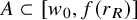 $A \subset [w_0,f(r_R)]$
, we define
$A \subset [w_0,f(r_R)]$
, we define
 $$ \begin{align} \mu_i(A) :=(r_i')^d\cdot \mathbb P(W\in A). \end{align} $$
When we cover with boxes in
 $\mathcal {P}_i$
on the spatial coordinate, the number
$\mathcal {P}_i$
on the spatial coordinate, the number
 $j_{\star }(i)$
of weight intervals in
$j_{\star }(i)$
of weight intervals in
 $\mathcal {H}(\mathcal {R})$
depends on i. In particular, for smaller side-length we do not include intervals of very large weights. This is because there are too few (or no) vertices of large weight in a typical box of small side-length, so we cannot control their number. We illustrate a hyperrectangle cover on Figure 4 in dimension
$\mathcal {H}(\mathcal {R})$
depends on i. In particular, for smaller side-length we do not include intervals of very large weights. This is because there are too few (or no) vertices of large weight in a typical box of small side-length, so we cannot control their number. We illustrate a hyperrectangle cover on Figure 4 in dimension
 $1$
. In IGIRG,
$1$
. In IGIRG,
 $\mu _i(A)$
is the expected number of vertices with weights in A in any box in
$\mu _i(A)$
is the expected number of vertices with weights in A in any box in
 $\mathcal {P}_i$
. In SFP,
$\mathcal {P}_i$
. In SFP,
 $\mu _i(A)$
is only roughly the expectation, since, for example, a box touching the boundary
$\mu _i(A)$
is only roughly the expectation, since, for example, a box touching the boundary
 $\partial Q$
in
$\partial Q$
in
 $\mathcal {P}_i$
may not contain exactly
$\mathcal {P}_i$
may not contain exactly
 $(r_i')^d$
vertices of
$(r_i')^d$
vertices of
 $\mathbb {Z}^d$
. By (2.13), all vertices in the hyperrectangle
$\mathbb {Z}^d$
. By (2.13), all vertices in the hyperrectangle
 $B^i(v) \times I_j$
are within distance
$B^i(v) \times I_j$
are within distance
 $r_i$
of v. Hence once we control the number of vertices in a dense set of hyperrectangles in all partitions
$r_i$
of v. Hence once we control the number of vertices in a dense set of hyperrectangles in all partitions
 $i\in [R]$
, we can find a net. We now define a hyperrectangle being ‘good’, with respect to a realisation of
$i\in [R]$
, we can find a net. We now define a hyperrectangle being ‘good’, with respect to a realisation of
 $\widetilde {\mathcal {V}}$
. Recall that
$\widetilde {\mathcal {V}}$
. Recall that
 $I(w)$
denotes the interval
$I(w)$
denotes the interval
 $I_j$
that contains w in Definition 2.8.
$I_j$
that contains w in Definition 2.8.
Definition 2.10. Consider the setting of Def. 2.13, and let a
 $ \mathcal {H}(\mathcal {R})$
be a hyperrectangle-cover of
$ \mathcal {H}(\mathcal {R})$
be a hyperrectangle-cover of
 $Q\times [w_0, f(r_R)]$
. Consider a realisation of the weighted vertex set
$Q\times [w_0, f(r_R)]$
. Consider a realisation of the weighted vertex set
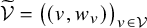 ${\widetilde {\mathcal {V}}} =\big ((v, w_v)\big )_{v\in \mathcal {V}}$
.
${\widetilde {\mathcal {V}}} =\big ((v, w_v)\big )_{v\in \mathcal {V}}$
.
We recursively define when we call a vertex
 ${\widetilde {v}}\in {\widetilde {\mathcal {V}}}$
and a box
${\widetilde {v}}\in {\widetilde {\mathcal {V}}}$
and a box
 $B\in {\widehat {\mathcal {P}}}(\mathcal {R})$
good. Every vertex is
$B\in {\widehat {\mathcal {P}}}(\mathcal {R})$
good. Every vertex is
 $1$
-good. For all
$1$
-good. For all
 $i \in [R]$
, we say a vertex
$i \in [R]$
, we say a vertex
 ${\tilde {v}}=(v, w_v)\in {\widetilde {\mathcal {V}}}$
is i-good if the boxes
${\tilde {v}}=(v, w_v)\in {\widetilde {\mathcal {V}}}$
is i-good if the boxes
 $B^1(v),\ldots ,B^{i-1}(v)$
are all good (which we define next). Denote the set of i-good (weighted) vertices by
$B^1(v),\ldots ,B^{i-1}(v)$
are all good (which we define next). Denote the set of i-good (weighted) vertices by
 ${\widetilde {\mathcal {G}}}_i:=\{{\widetilde {v}} \in {\widetilde {\mathcal {V}}} \ i\text {-good}\}$
and
${\widetilde {\mathcal {G}}}_i:=\{{\widetilde {v}} \in {\widetilde {\mathcal {V}}} \ i\text {-good}\}$
and
 $\mathcal {G}_i:=\{v: {\widetilde {v}} \in {\widetilde {\mathcal {G}}}_i\}$
. We say that a box
$\mathcal {G}_i:=\{v: {\widetilde {v}} \in {\widetilde {\mathcal {G}}}_i\}$
. We say that a box
 $B \in \mathcal {P}_i$
is i-good or simply good if the following conditions all hold:
$B \in \mathcal {P}_i$
is i-good or simply good if the following conditions all hold:
-
(B1) Either
$i=1$
, or B contains at least
$1-\tfrac {2\delta }{R}\cdot (r_i'/r_{i-1}')^d$
many
$i-1$
-good sub-boxes
$B'\in \mathcal {P}_{i-1}$
. -
(B2) The total number of i-good vertices in B satisfies
(2.18)
$$ \begin{align} |\mathcal{G}_i \cap B | \in \left[\left(\frac{1}{2} - \frac{2(i-1)\delta}{R}\right)(r_i')^d, 2(r_i')^d\right]. \end{align} $$
-
(B3) For all
$w \in [w_0,f_{R,\delta }(r_i)]$
, the number of i-good vertices in B with weight in
$I(w)$
satisfies (2.19)
$$ \begin{align} |\widetilde{\mathcal{G}_i}\cap (B\times I(w))| \in \left[\frac{1}{8} \left(1 - \frac{2i\delta}{R}\right)\mu_i(I(w)), 8\mu_i(I(w))\right]. \end{align} $$


We say that the realisation
 $\widetilde {\mathcal {V}}$
is good with respect to the hyperrectangle-cover
$\widetilde {\mathcal {V}}$
is good with respect to the hyperrectangle-cover
 $\widetilde {\mathcal {P}}(\mathcal {R})$
if Q is R-good.
$\widetilde {\mathcal {P}}(\mathcal {R})$
if Q is R-good.
The above definition is not circular; the definition of i-good vertices depends only on the definition of good boxes in
 $\mathcal {P}_{i-1}$
, that is, one level lower, and then the definition of a good box in
$\mathcal {P}_{i-1}$
, that is, one level lower, and then the definition of a good box in
 $\mathcal {P}_i$
depends only on the number of i-good vertices in it (and their weights) and its number of good subboxes in
$\mathcal {P}_i$
depends only on the number of i-good vertices in it (and their weights) and its number of good subboxes in
 $\mathcal {P}_{i-1}$
. For
$\mathcal {P}_{i-1}$
. For
 $i=1$
, the (longer) definition of
$i=1$
, the (longer) definition of
 $1$
-good vertices is vacuous, so every vertex is indeed
$1$
-good vertices is vacuous, so every vertex is indeed
 $1$
-good which we emphasised in the definition. Further,
$1$
-good which we emphasised in the definition. Further,
 $\mathcal {G}_R\subseteq \mathcal {G}_{R-1}\subseteq \ldots \subseteq \mathcal {G}_1=\mathcal {V}\cap Q$
, since each i-good vertex is also
$\mathcal {G}_R\subseteq \mathcal {G}_{R-1}\subseteq \ldots \subseteq \mathcal {G}_1=\mathcal {V}\cap Q$
, since each i-good vertex is also
 $(i\!-\!1)$
-good for all
$(i\!-\!1)$
-good for all
 $i\le R$
. See Figure 4 for a graphical depiction of i-good vertices and boxes.
$i\le R$
. See Figure 4 for a graphical depiction of i-good vertices and boxes.
Before we relate goodness to our overall goal of finding an
 $(\delta ,\mathcal {R})$
-net, we give some easy algebraic bounds which we need multiple times in the rest of the section. Recall that
$(\delta ,\mathcal {R})$
-net, we give some easy algebraic bounds which we need multiple times in the rest of the section. Recall that
 $I(w)=I_j$
iff
$I(w)=I_j$
iff
 $w\in I_j$
(cf. Def. 2.8) and that
$w\in I_j$
(cf. Def. 2.8) and that
 $\mu _i(A)=(r_i')^d\cdot \mathbb P(W\in A)$
in (2.17).
$\mu _i(A)=(r_i')^d\cdot \mathbb P(W\in A)$
in (2.17).
Lemma 2.11. Consider the setting of Proposition 2.5 and Definitions 2.6, 2.13. Suppose
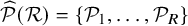 $\widehat {\mathcal {P}}(\mathcal {R})= \{\mathcal {P}_1,\ldots ,\mathcal {P}_R\}$
is an
$\widehat {\mathcal {P}}(\mathcal {R})= \{\mathcal {P}_1,\ldots ,\mathcal {P}_R\}$
is an
 $\mathcal {R}$
-partition of Q, and for all
$\mathcal {R}$
-partition of Q, and for all
 $i \in [R]$
, let
$i \in [R]$
, let
 $r_i'$
be the side length of boxes in
$r_i'$
be the side length of boxes in
 $\mathcal {P}_i$
. Then for all
$\mathcal {P}_i$
. Then for all
 $i \in [R]$
and all
$i \in [R]$
and all
 $w \in [w_0,f(r_R)]$
, we have
$w \in [w_0,f(r_R)]$
, we have
 $$ \begin{align} r_i^d\ell(w)w^{-(\tau-1)}/(2d)^{\tau+d+1} &\le \mu_i(I(w))= (r_i')^d \cdot \mathbb{P}(W\in I(w)) \le 2^\tau r_i^d\ell(w)w^{-(\tau-1)}, \end{align} $$
 $$ \begin{align} r_i^d \ell(f(r_i)) f(r_i)^{-(\tau-1)} &\ge (2d)^{2\tau+d+8}\log(16R/\delta). \end{align} $$
Proof. We start by showing (2.20). We write
 $I(w) = [w_-, w_+)$
. The definition of a base-
$I(w) = [w_-, w_+)$
. The definition of a base-
 $2$
-cover (Definition 2.8) ensures that
$2$
-cover (Definition 2.8) ensures that
 $w_-,w_+ \in [w/2,2w]$
and
$w_-,w_+ \in [w/2,2w]$
and
 $w_+/w_-=2$
. Thus by the lower bound (2.1) on
$w_+/w_-=2$
. Thus by the lower bound (2.1) on
 $w_0$
, for all
$w_0$
, for all
 $w\in [w_0, f(r_R)]$
,
$w\in [w_0, f(r_R)]$
,
 $$ \begin{align*} \mathbb{P}(W \in I(w)) &= \ell(w_-)w_-^{-(\tau-1)} - \ell(w_+)w_+^{-(\tau-1)}\\ &\ge \ell(w)\left(\frac{99}{100}w_-^{-(\tau-1)} - \frac{101}{100}w_+^{-(\tau-1)}\right)\\ &= \ell(w)w_-^{-(\tau-1)}\left(\frac{99}{100} - \frac{101}{100}\cdot 2^{-(\tau-1)}\right). \end{align*} $$
Since
 $\tau> 2$
and
$\tau> 2$
and
 $w_- \le w$
, it follows that
$w_- \le w$
, it follows that
 $\mu _i(I(w)) \ge (r_i')^d\ell (w) w^{-(\tau -1)}/2^{\tau +1}$
. The required lower bound on
$\mu _i(I(w)) \ge (r_i')^d\ell (w) w^{-(\tau -1)}/2^{\tau +1}$
. The required lower bound on
 $\mu _i(I(w))$
then follows by the lower bound (P1) in Definition 2.6 on
$\mu _i(I(w))$
then follows by the lower bound (P1) in Definition 2.6 on
 $r_i'$
. By a very similar argument to the lower bound, (2.1) also implies that
$r_i'$
. By a very similar argument to the lower bound, (2.1) also implies that
 $$ \begin{align*} \mathbb{P}(W \in I(w)) \le \frac{101}{100}\ell(w)w_-^{-(\tau-1)} \le 2^\tau\ell(w)w^{-(\tau-1)}, \end{align*} $$
so the required upper bound on
 $\mu _i(I(w))$
likewise follows by the upper bound (P1) on
$\mu _i(I(w))$
likewise follows by the upper bound (P1) on
 $r_i'$
. It remains to show (2.21). First we show that
$r_i'$
. It remains to show (2.21). First we show that
 $f(r_R) \ge f(r_{R-1}) \ge \ldots \ge f(r_1) \ge w_0$
. Indeed, let
$f(r_R) \ge f(r_{R-1}) \ge \ldots \ge f(r_1) \ge w_0$
. Indeed, let
 $j \in [R]$
. By the definition of f in (2.3),
$j \in [R]$
. By the definition of f in (2.3),
 $$ \begin{align} \frac{f(r_j)}{f(r_{j-1})} = \left(\frac{r_j}{r_{j-1}}\right)^{d/(\tau-1)} \cdot \left(\frac{1 \wedge \inf\big\{\ell(x)\colon x \in [w_0,r_j^{d/(\tau-1)}]\big\}}{1 \wedge \inf\big\{\ell(x)\colon x \in [w_0,r_{j-1}^{d/(\tau-1)}]\big\}}\right)^{1/(\tau-1)}. \end{align} $$
To bound the second factor, we will first observe that since
 $r_{j-1} \le r_j$
, we have
$r_{j-1} \le r_j$
, we have
 $\inf \{\ell (x)\colon x \in [w_0,r_j^{d/(\tau -1)}]\} \le \inf \{\ell (x)\colon x \in [w_0,r_{j-1}^{d/(\tau -1)}]\}$
. By considering the two possible values of
$\inf \{\ell (x)\colon x \in [w_0,r_j^{d/(\tau -1)}]\} \le \inf \{\ell (x)\colon x \in [w_0,r_{j-1}^{d/(\tau -1)}]\}$
. By considering the two possible values of
 $1 \wedge \inf \{\ell (x)\colon x \in [w_0,r_j^{d/(\tau -1)}]\}$
separately, it follows that we can drop the minimum with
$1 \wedge \inf \{\ell (x)\colon x \in [w_0,r_j^{d/(\tau -1)}]\}$
separately, it follows that we can drop the minimum with
 $1$
in the ratio:
$1$
in the ratio:
 $$ \begin{align} \left(\frac{1 \wedge \inf\big\{\ell(x)\colon x \in [w_0,r_j^{d/(\tau-1)}]\big\}}{1 \wedge \inf\big\{\ell(x)\colon x \in [w_0,r_{j-1}^{d/(\tau-1)}]\big\}}\right)^{1/(\tau-1)} \ge \left(\frac{\inf\big\{\ell(x)\colon x \in [w_0,r_j^{d/(\tau-1)}]\big\}}{\inf\big\{\ell(x)\colon x \in [w_0,r_{j-1}^{d/(\tau-1)}]\big\}}\right)^{1/(\tau-1)}. \end{align} $$
We now bound
 $\ell (x)$
on
$\ell (x)$
on
 $[w_0, r_{j-1}^{d/(\tau -1)}]$
(in the denominator) by repeatedly applying (2.1). We write
$[w_0, r_{j-1}^{d/(\tau -1)}]$
(in the denominator) by repeatedly applying (2.1). We write
 $\lg (\cdot )=\log _2(\cdot )$
. Then, we have
$\lg (\cdot )=\log _2(\cdot )$
. Then, we have
 $r_j^{d/(\tau -1)} = 2^{\lg ((r_j/r_{j-1} )^{d/(\tau -1)})} r_{j-1}^{d/(\tau -1)}$
, so we iterate the bound in (2.1) roughly
$r_j^{d/(\tau -1)} = 2^{\lg ((r_j/r_{j-1} )^{d/(\tau -1)})} r_{j-1}^{d/(\tau -1)}$
, so we iterate the bound in (2.1) roughly
 $\lg ((r_j/r_{j-1} )^{d/(\tau -1)})$
many times to obtain that for all
$\lg ((r_j/r_{j-1} )^{d/(\tau -1)})$
many times to obtain that for all
 $x \in [r_{j-1}^{d/(\tau -1)}, r_j^{d/(\tau -1)}]$
we have
$x \in [r_{j-1}^{d/(\tau -1)}, r_j^{d/(\tau -1)}]$
we have
 $$\begin{align*}\ell(x) \ge \left(\frac{99}{100}\right)^{1 + \lg ((r_j/r_{j-1} )^{d/(\tau-1)})} \ell(r_{j-1}). \end{align*}$$
Returning to (2.23), the ratio of the two infima in the smaller interval
 $[w_0,r_{j-1}^{d/(\tau -1)}]$
is one. And since
$[w_0,r_{j-1}^{d/(\tau -1)}]$
is one. And since
 $r_j \ge 2r_{j-1}$
by (R2) of Definition 2.4 (using
$r_j \ge 2r_{j-1}$
by (R2) of Definition 2.4 (using
 $\delta <1/16 < 1$
), it follows that
$\delta <1/16 < 1$
), it follows that
 $$ \begin{align*} &\left(\frac{\inf\big\{\ell(x)\colon x \in [w_0,r_j^{d/(\tau-1)}]\big\}}{\inf\big\{\ell(x)\colon x \in [w_0,r_{j-1}^{d/(\tau-1)}]\big\}}\right)^{1/(\tau-1)} \ge \left(\frac{99}{100}\right)^{1 + \lg ((r_j/r_{j-1} )^{d/(\tau-1)}) } \\ &\qquad\qquad \qquad\ge \left(\frac{1}{2}\right)^{\frac{1}{\tau-1}\lg ((r_j/r_{j-1} )^{d/(\tau-1)}) } = \left(\frac{r_{j-1}}{r_j}\right)^{d/(\tau-1)^2}. \end{align*} $$
Combining this with (2.22), (2.23), and the fact that
 $\tau> 2$
, we obtain
$\tau> 2$
, we obtain
 $$\begin{align*}\frac{f(r_j)}{f(r_{j-1})} \ge \left(\frac{r_j}{r_{j-1}}\right)^{\frac{d}{\tau-1}(1-1/(\tau-1))} \ge 1. \end{align*}$$
Hence
 $f(r_R) \ge f(r_{R-1}) \ge \ldots \ge f(r_1)$
, as claimed. It is now relatively easy to prove the desired lower bound. From the definition of f in (2.3), we have
$f(r_R) \ge f(r_{R-1}) \ge \ldots \ge f(r_1)$
, as claimed. It is now relatively easy to prove the desired lower bound. From the definition of f in (2.3), we have
 $f(r_i) \le r_i^{d/(\tau -1)}$
, and (2.5) in the definition of well-spacedness ensures that
$f(r_i) \le r_i^{d/(\tau -1)}$
, and (2.5) in the definition of well-spacedness ensures that
 $f(r_i)\ge w_0$
, so
$f(r_i)\ge w_0$
, so
 $$ \begin{align*} \ell(f(r_i))f(r_i)^{-(\tau-1)} & = \frac{\ell(f(r_i))}{1 \wedge \inf\{\ell(x)\colon x \in [w_0,r_i^{d/(\tau-1)}]\}} \cdot \frac{(2d)^{2\tau+d+8}\log(16R/\delta)}{r_i^d} \\ &\ge \frac{(2d)^{2\tau+d+8}\log(16R/\delta)}{r_i^d}. \end{align*} $$
Multiplying by
 $r_i^d$
finishes the statement of (2.21).
$r_i^d$
finishes the statement of (2.21).
We now show that given that the box Q is good with respect to a hyperrectangle cover, we can find an
 $(\delta ,\mathcal {R})$
-net for Q (see Def. 2.3).
$(\delta ,\mathcal {R})$
-net for Q (see Def. 2.3).
Lemma 2.12. Consider the setting of Proposition 2.5 and Definitions 2.6, 2.13, 2.10, that is, a hyper-rectangle cover
 $ {\mathcal {H}}(\mathcal {R})$
of
$ {\mathcal {H}}(\mathcal {R})$
of
 $Q\times [w_0, f(r_R)]$
, and a realisation of
$Q\times [w_0, f(r_R)]$
, and a realisation of
 $\widetilde {\mathcal {V}}$
for which Q is R-good. Then
$\widetilde {\mathcal {V}}$
for which Q is R-good. Then
 $\widetilde {\mathcal {G}}_R$
, the set of all R-good vertices, forms an
$\widetilde {\mathcal {G}}_R$
, the set of all R-good vertices, forms an
 $(\delta ,\mathcal {R})$
-net for Q.
$(\delta ,\mathcal {R})$
-net for Q.
Proof. Suppose that Q is R-good. The side length of Q equals
 $r_R'$
by (P3) in Def. 2.6, and
$r_R'$
by (P3) in Def. 2.6, and
 $\delta \in (0,1/16)$
in the setting of Proposition 2.5, hence we may apply (B2) in Def. 2.10 for
$\delta \in (0,1/16)$
in the setting of Proposition 2.5, hence we may apply (B2) in Def. 2.10 for
 $i=R$
to get
$i=R$
to get
 $$\begin{align*}|\widetilde{\mathcal{G}}_R| \ge \left(\frac{1}{2} - \frac{2(R-1)\delta}{R}\right)\mathrm{Vol}(Q) \ge \left(\frac{1}{2} - 2\delta\right)\mathrm{Vol}(Q)> \mathrm{Vol}(Q)/4, \end{align*}$$
hence the cardinality assumption in Definition 2.3 is satisfied for
 $\widetilde {\mathcal {G}}_R$
. Recall that
$\widetilde {\mathcal {G}}_R$
. Recall that
 $B^i(v)$
is the box in
$B^i(v)$
is the box in
 $\mathcal {P}_i$
containing v. To show that
$\mathcal {P}_i$
containing v. To show that
 $\widetilde {\mathcal {G}}_R$
satisfies Definitions 2.3, we first show that for all
$\widetilde {\mathcal {G}}_R$
satisfies Definitions 2.3, we first show that for all
 $v\in \mathcal {G}_R$
,
$v\in \mathcal {G}_R$
,
 $$ \begin{align} \mathcal{G}_i \cap B^i(v)= \mathcal{G}_R \cap B^i(v). \end{align} $$
To show this, we need to show that every i-good vertex
 $u \in B^i(v)$
is also R-good, that is, that
$u \in B^i(v)$
is also R-good, that is, that
 $B^j(u)$
is good for all
$B^j(u)$
is good for all
 $j \in [R]$
. By the definition of i-goodness (Def. 2.10),
$j \in [R]$
. By the definition of i-goodness (Def. 2.10),
 $B^j(u)$
is good for all
$B^j(u)$
is good for all
 $j \le i-1$
, and
$j \le i-1$
, and
 $B^R(u) = Q$
is good by hypothesis. Consider now a
$B^R(u) = Q$
is good by hypothesis. Consider now a
 $j \in [i+1, R-1]$
. By Def. 2.6, the partition
$j \in [i+1, R-1]$
. By Def. 2.6, the partition
 $\mathcal {P}_i$
is a refinement of the partition
$\mathcal {P}_i$
is a refinement of the partition
 $\mathcal {P}_j$
, so
$\mathcal {P}_j$
, so
 $B^j(u) = B^j(v)$
. Since v is R-good, it follows that
$B^j(u) = B^j(v)$
. Since v is R-good, it follows that
 $B^j(u)$
is good. So,
$B^j(u)$
is good. So,
 $B^j(u)$
is good for all
$B^j(u)$
is good for all
 $j \in [R]$
, so u is R-good, showing (2.24).
$j \in [R]$
, so u is R-good, showing (2.24).
With
 $I(w)\subseteq [w/2, 2w]$
being the interval containing w in the base-
$I(w)\subseteq [w/2, 2w]$
being the interval containing w in the base-
 $2$
-cover of
$2$
-cover of
 $[w_0, f(r_i)]$
in Def.2.8, we now argue that
$[w_0, f(r_i)]$
in Def.2.8, we now argue that
 $$ \begin{align*} | \widetilde {\mathcal{G}}_R \cap (B_{r_i}(v) \times [w/2,2w])| \ge |\widetilde {\mathcal{G}}_R \cap (B^i(v)\times I(w))|=|\widetilde {\mathcal{G}}_i \cap (B^i(v)\times I(w))|. \end{align*} $$
Indeed,
 $B^{i}(v)\subseteq B_{r_i}(v)$
by (2.13) and
$B^{i}(v)\subseteq B_{r_i}(v)$
by (2.13) and
 $I(w)\subseteq [w/2, 2w]$
by Def. 2.8, and since all i-good vertices in
$I(w)\subseteq [w/2, 2w]$
by Def. 2.8, and since all i-good vertices in
 $B^i(v)$
are also R-good by (2.24), the statement follows. Now we apply, on the right-hand side
$B^i(v)$
are also R-good by (2.24), the statement follows. Now we apply, on the right-hand side
 $|\widetilde {\mathcal {G}_i} \cap (B^i(v) \times I(w))|$
above, the lower bound (2.19) from Def. 2.10 (B3), then (2.20) to obtain
$|\widetilde {\mathcal {G}_i} \cap (B^i(v) \times I(w))|$
above, the lower bound (2.19) from Def. 2.10 (B3), then (2.20) to obtain
 $$ \begin{align*} \big| \widetilde{\mathcal{G}}_R\cap (B^{i}(v)\times [w/2,2w])\big| &\ {\buildrel ({\scriptstyle 2.19}) \over \ge}\ \frac18\left(1-\frac{2i\delta}{R}\right) \mu_i(I(w)) \\&\ {\buildrel ({\scriptstyle 2.20}) \over \ge} \frac{1}{8} \left(1-\frac{2i\delta}{R}\right)r_i^d\ell(w)w^{-(\tau-1)}/(2d)^{\tau+d+1}. \end{align*} $$
Observing that
 $\delta <1/16$
and
$\delta <1/16$
and
 $i\le R$
ensures that the prefactor on the right-hand side of the last row is at least
$i\le R$
ensures that the prefactor on the right-hand side of the last row is at least
 $1/8\cdot 1/2=1/2^4$
, establishing (2.4) for all
$1/8\cdot 1/2=1/2^4$
, establishing (2.4) for all
 $w\le f(r_i)$
, as required.
$w\le f(r_i)$
, as required.
A lower bound on the probability that any given box in an
 $\mathcal {R}$
-partition is good, together with Lemma 2.7 and Lemma 2.12, will yield the proof of Proposition 2.5. The bound is by induction on i together with Chernoff bounds. Recall I and
$\mathcal {R}$
-partition is good, together with Lemma 2.7 and Lemma 2.12, will yield the proof of Proposition 2.5. The bound is by induction on i together with Chernoff bounds. Recall I and
 $I(w)$
from Def. 2.8, applied to the interval
$I(w)$
from Def. 2.8, applied to the interval
 $[w_0,f(r_R)]$
for
$[w_0,f(r_R)]$
for
 $\mathcal {R}=\{r_1, \ldots , r_R\}$
. Recall that (2.19) of Def. 2.10 (B3) is required only when
$\mathcal {R}=\{r_1, \ldots , r_R\}$
. Recall that (2.19) of Def. 2.10 (B3) is required only when
 $w\in [w_0, f(r_i)]$
, and that
$w\in [w_0, f(r_i)]$
, and that
 $j_\star (i)$
in (2.16) is the index of
$j_\star (i)$
in (2.16) is the index of
 $I_j$
that contains
$I_j$
that contains
 $f(r_i)$
. We now gradually reveal vertex-weights by giving a weight-revealment scheme. Here, we aim for unified proof that works for SFP and IGIRG simultaneously. In IGIRG we can make use the independence property of marked Poisson point processes, namely, that the number of vertices in
$f(r_i)$
. We now gradually reveal vertex-weights by giving a weight-revealment scheme. Here, we aim for unified proof that works for SFP and IGIRG simultaneously. In IGIRG we can make use the independence property of marked Poisson point processes, namely, that the number of vertices in
 $B\times I_j$
and
$B\times I_j$
and
 $A\times I_{j'}$
are independent if
$A\times I_{j'}$
are independent if
 $j\neq j'$
, see [Reference Last and Penrose61]. However, in SFP this is not the case and we may run out of vertices as we gradually reveal vertices with higher and higher weights. To solve this issue, we first reveal all vertex positions only (one could think of this as a sigma-algebra, we call it
$j\neq j'$
, see [Reference Last and Penrose61]. However, in SFP this is not the case and we may run out of vertices as we gradually reveal vertices with higher and higher weights. To solve this issue, we first reveal all vertex positions only (one could think of this as a sigma-algebra, we call it
 $\mathcal {F}_0$
and leave vertex-weights yet unrevealed. Then, in subsequent weight-revealment steps
$\mathcal {F}_0$
and leave vertex-weights yet unrevealed. Then, in subsequent weight-revealment steps
 $\mathcal {F}_1, \mathcal {F}_2, \dots , \mathcal {F}_R$
, we reveal the vertex-weights of those vertices whose weight falls into the intervals
$\mathcal {F}_1, \mathcal {F}_2, \dots , \mathcal {F}_R$
, we reveal the vertex-weights of those vertices whose weight falls into the intervals
 $I_j$
, with the maximal j revealed increasing along the steps. Recall that
$I_j$
, with the maximal j revealed increasing along the steps. Recall that
 $j_\star (i)$
is the index of the interval
$j_\star (i)$
is the index of the interval
 $I_j$
containing
$I_j$
containing
 $f(r_i)$
from (2.16), and that we denote the
$f(r_i)$
from (2.16), and that we denote the
 $\sigma $
-algebra generated by a random variables
$\sigma $
-algebra generated by a random variables
 $X,Y$
by
$X,Y$
by
 $\sigma (X, Y)$
.
$\sigma (X, Y)$
.
Definition 2.13. Consider the setting of Proposition 2.5 and Definitions 2.6, 2.13. Suppose
 $\mathcal {H}(\mathcal {R})$
is a hyperrectangle-cover of
$\mathcal {H}(\mathcal {R})$
is a hyperrectangle-cover of
 $Q\times [w_0, f(r_R)]$
. Let
$Q\times [w_0, f(r_R)]$
. Let
 $\widetilde {\mathcal {V}}$
be a realisation of the weighted vertices in Definition 1.3 and B be a box in one of the partitions
$\widetilde {\mathcal {V}}$
be a realisation of the weighted vertices in Definition 1.3 and B be a box in one of the partitions
 $(\mathcal {P}_i)_{i\le R}$
. We define
$(\mathcal {P}_i)_{i\le R}$
. We define
$$ \begin{align} \mathcal{F}_{i}(B):= \begin{cases} \sigma(\mathcal{V}\cap B) & \text{for }i=0,\\ \sigma\left(\mathcal{F}_0(B),\widetilde{\mathcal{V}} \cap (B\times \cup_{j\le j_\star(i)}I_j\right) & \text{for all } 1\le i\le R. \end{cases} \end{align} $$
We say that we vertices with weight in
 $\cup _{j\le j_\star (i)}I_j$
have ‘revealed’ weight in
$\cup _{j\le j_\star (i)}I_j$
have ‘revealed’ weight in
 $\mathcal {F}_{i}$
, while the vertices in
$\mathcal {F}_{i}$
, while the vertices in
 $[1,\infty )\setminus \cup _{j\le j_\star (i)}I_j$
have ‘unrevealed’ weight in
$[1,\infty )\setminus \cup _{j\le j_\star (i)}I_j$
have ‘unrevealed’ weight in
 $\mathcal {F}_{i}$
. We denote by
$\mathcal {F}_{i}$
. We denote by
 $\mathcal {X}_i(B)$
the outcome of the revealment scheme
$\mathcal {X}_i(B)$
the outcome of the revealment scheme
 $\mathcal {F}_i(B)$
:
$\mathcal {F}_i(B)$
:
 $\mathcal {X}_i(B)$
contains the position of all vertices in the box B, where a subset of these vertices is marked by the revealed vertex-weight.
$\mathcal {X}_i(B)$
contains the position of all vertices in the box B, where a subset of these vertices is marked by the revealed vertex-weight.
 $\mathcal {F}_0(B)$
reveals the number and positions of vertices in B, while
$\mathcal {F}_0(B)$
reveals the number and positions of vertices in B, while
 $\mathcal {F}_{i-1}(B)$
reveals the precise weights only of vertices whose weight falls in the interval
$\mathcal {F}_{i-1}(B)$
reveals the precise weights only of vertices whose weight falls in the interval
 $\cup _{j\le j_\star (i-1)}I_j \supseteq [w_0, f(r_{i-1})]$
. Note that the weight distribution of vertices with unrevealed weight changes along the revealment procedure, since after revealment step
$\cup _{j\le j_\star (i-1)}I_j \supseteq [w_0, f(r_{i-1})]$
. Note that the weight distribution of vertices with unrevealed weight changes along the revealment procedure, since after revealment step
 $i-1$
it is the conditional weight distribution that the weight does not fall in the revealed interval
$i-1$
it is the conditional weight distribution that the weight does not fall in the revealed interval
 $\cup _{j\le j_\star (i-1)}I_j$
. The fact that
$\cup _{j\le j_\star (i-1)}I_j$
. The fact that
 $\mathcal {R}$
is
$\mathcal {R}$
is
 $\delta $
-well-spaced, means that vertex weights between
$\delta $
-well-spaced, means that vertex weights between
 $w_0 2^{j_\star (i-1)}\approx f(r_{i-1})$
and
$w_0 2^{j_\star (i-1)}\approx f(r_{i-1})$
and
 $f(r_i)$
are not revealed in
$f(r_i)$
are not revealed in
 $\mathcal {F}_{i-1}(B)$
. Also, vertex weights in
$\mathcal {F}_{i-1}(B)$
. Also, vertex weights in
 $[1,w_0)$
are not revealed at all; since
$[1,w_0)$
are not revealed at all; since
 $w_0$
is large,
$w_0$
is large,
 $\mathbb {P}(W\le w_0)$
is large and most vertex weights will not be revealed by exposing
$\mathbb {P}(W\le w_0)$
is large and most vertex weights will not be revealed by exposing
 $\mathcal {F}_{i-1}(B)$
. The filtration generated by
$\mathcal {F}_{i-1}(B)$
. The filtration generated by
 $\mathcal {F}_{i-1}(B)$
thus determines whether or not boxes in
$\mathcal {F}_{i-1}(B)$
thus determines whether or not boxes in
 $ \cup _{j\le i-1} \mathcal {P}_{j}$
are good, and whether or not a vertex is i-good (see Def. 2.10), since i-goodness of a vertex only depends on boxes with index at most
$ \cup _{j\le i-1} \mathcal {P}_{j}$
are good, and whether or not a vertex is i-good (see Def. 2.10), since i-goodness of a vertex only depends on boxes with index at most
 $i-1$
containing the vertex. So,
$i-1$
containing the vertex. So,
 $\mathcal {F}_{i-1}(B)$
determines whether or not
$\mathcal {F}_{i-1}(B)$
determines whether or not
 $B\in \mathcal {P}_i$
satisfies Def. 2.10 (B1) -(B2), but it leaves (B3) undecided for weights slightly below
$B\in \mathcal {P}_i$
satisfies Def. 2.10 (B1) -(B2), but it leaves (B3) undecided for weights slightly below
 $f(r_i)$
. The next lemma treats (B3), with
$f(r_i)$
. The next lemma treats (B3), with
 $\mathcal {F}_{i-1}(B)$
exposed.
$\mathcal {F}_{i-1}(B)$
exposed.
Lemma 2.14. Consider the setting of Proposition 2.5 and Definitions 2.6, 2.13. Let
 $\mathcal {H}(\mathcal {R})$
be a hyperrectangle-cover of the cube Q. Let
$\mathcal {H}(\mathcal {R})$
be a hyperrectangle-cover of the cube Q. Let
 $i \in [R]$
and let
$i \in [R]$
and let
 $B \in \mathcal {P}_i$
. Let X be a realisationFootnote
9
of
$B \in \mathcal {P}_i$
. Let X be a realisationFootnote
9
of
 $\mathcal {X}_{i-1}(B)$
that satisfies Definition 2.10 (B1) and (B2) for B. Then independently of other boxes in
$\mathcal {X}_{i-1}(B)$
that satisfies Definition 2.10 (B1) and (B2) for B. Then independently of other boxes in
 $\mathcal {P}_i$
, uniformly for all such X,
$\mathcal {P}_i$
, uniformly for all such X,
 $$ \begin{align} \mathbb{P}(B\text{ is good}\mid \mathcal{X}_{i-1}(B) = X) \ge 1 - \delta/(2R). \end{align} $$
Proof. Recall
 $I_j$
from Def. 2.8, and let
$I_j$
from Def. 2.8, and let
 $B\in \mathcal {P}_i$
. Let
$B\in \mathcal {P}_i$
. Let
 $$ \begin{align} a(I_j) := (1-2i\delta/R)\mu_i(I_j)/8, \qquad b(I_j) := 8\mu_i(I_j) \end{align} $$
be the required lower and upper bounds in (2.19). Let
 $\Xi _j(B)=|\widetilde {\mathcal {G}_i}\cap (B\times I_j)|$
; thus (B3) holds for
$\Xi _j(B)=|\widetilde {\mathcal {G}_i}\cap (B\times I_j)|$
; thus (B3) holds for
 $B\times I_j$
iff
$B\times I_j$
iff
 $\Xi _j(B) \in [a(I_j),b(I_j)]$
. Since B satisfies (B1)–(B2) on X, by a union bound,
$\Xi _j(B) \in [a(I_j),b(I_j)]$
. Since B satisfies (B1)–(B2) on X, by a union bound,
 $$ \begin{align} \mathbb{P}\big(B\text{ is good}\mid \mathcal{X}_{i-1}(B) = X\big) \ge 1 - \sum_{I_j: j\le j_\star(i)} \mathbb{P}\big(\Xi_j(B) \notin [a(I_j),b(I_j)] \mid \mathcal{X}_{i-1}(B) = X \big). \end{align} $$
We proceed by bounding each term above. By the definition of
 $\mathcal {F}_{i-1}(B)$
in (2.25), we already exposed
$\mathcal {F}_{i-1}(B)$
in (2.25), we already exposed
 $\Xi _j(B)$
when
$\Xi _j(B)$
when
 $i> 1$
and
$i> 1$
and
 $j\le j_*(i-1)$
; the latter is equivalent to
$j\le j_*(i-1)$
; the latter is equivalent to
 $\min (I_j) \le f(r_{i-1})$
.
$\min (I_j) \le f(r_{i-1})$
.
Case 1:
 $\boldsymbol {i \!>\! 1}$
and
$\boldsymbol {i \!>\! 1}$
and
 $\boldsymbol {j\!\le \! j_\star (i\!-\!1)}$
. We first show that
$\boldsymbol {j\!\le \! j_\star (i\!-\!1)}$
. We first show that
 $\Xi _j \ge a(I_j)$
holds deterministically on
$\Xi _j \ge a(I_j)$
holds deterministically on
 $\{\mathcal {X}_{i-1}(B)=X\}$
. The goodness of each sub-box
$\{\mathcal {X}_{i-1}(B)=X\}$
. The goodness of each sub-box
 $B'\in \mathcal {P}_{i-1}$
of
$B'\in \mathcal {P}_{i-1}$
of
 $B\in \mathcal {P}_i$
is revealed by
$B\in \mathcal {P}_i$
is revealed by
 $\mathcal {F}_{i-1}(B)$
. If
$\mathcal {F}_{i-1}(B)$
. If
 $B'\in \mathcal {P}_{i-1}$
is a good box, all vertices in
$B'\in \mathcal {P}_{i-1}$
is a good box, all vertices in
 $\mathcal {G}_{i-1} \cap B'$
are also i-good by Definition 2.10. So
$\mathcal {G}_{i-1} \cap B'$
are also i-good by Definition 2.10. So
 $$ \begin{align} \Xi_j(B) = |\widetilde{\mathcal{G}_i}\cap (B\times I_j)|\ge \sum_{B'\in \mathcal{P}_{i-1}\colon B' \text{ good}} |\widetilde{\mathcal{G}}_{i-1}\cap (B'\times I_j)|. \end{align} $$
Since
 $j\le j_\star (i-1)$
,
$j\le j_\star (i-1)$
,
 $\min (I_j) \le f(r_{i-1})$
, so we may apply (2.19) to the good subboxes:
$\min (I_j) \le f(r_{i-1})$
, so we may apply (2.19) to the good subboxes:
 $$ \begin{align} |\widetilde{\mathcal{G}}_{i-1}\cap (B'\times I_j)|\ge \left(1-\frac{2(i-1)\delta}{R}\right)\frac{\mu_{i-1}(I_j)}{8} = \left(1-\frac{2(i-1)\delta}{R}\right)\frac{\mu_i(I_j)}{8}\left(\frac{r_{i-1}'}{r_i'}\right)^d, \end{align} $$
where
 $\mu _i(I_j)/\mu _{i-1}(I_j)=(r_i'/r_{i-1}')^d$
follows from (2.17). By (B1) holding on X, B contains at least
$\mu _i(I_j)/\mu _{i-1}(I_j)=(r_i'/r_{i-1}')^d$
follows from (2.17). By (B1) holding on X, B contains at least
 $(1-2\delta /R)(r_i'/r_{i-1}')^d$
good sub-boxes in
$(1-2\delta /R)(r_i'/r_{i-1}')^d$
good sub-boxes in
 $\mathcal {P}_{i-1}$
. Combining that with (2.29)–(2.30) and (2.27) yields
$\mathcal {P}_{i-1}$
. Combining that with (2.29)–(2.30) and (2.27) yields
 $$ \begin{align*} \begin{aligned} \Xi_j(B)&\ge \left(1-\frac{2\delta}{R}\right) \cdot \left(1-\frac{2(i-1)\delta}{R}\right) \frac{\mu_i(I_j)}{8} \ge \left(1-\frac{2i\delta}{R}\right) \frac{\mu_i(I_j)}{8} = a(I_j). \end{aligned} \end{align*} $$
We show
 $\Xi _j(B)=|\widetilde {\mathcal {G}_i}\cap (B\times I_j)| \le b(I_j)$
also holds a.s. B contains
$\Xi _j(B)=|\widetilde {\mathcal {G}_i}\cap (B\times I_j)| \le b(I_j)$
also holds a.s. B contains
 $(r_i'/r_{i-1}')^d$
sub-boxes in
$(r_i'/r_{i-1}')^d$
sub-boxes in
 $\mathcal {P}_{i-1}$
by Def. 2.6 (P2). If a sub-box is bad, it contains no i-good vertices. If it is good, (B3) holds and it contains at most
$\mathcal {P}_{i-1}$
by Def. 2.6 (P2). If a sub-box is bad, it contains no i-good vertices. If it is good, (B3) holds and it contains at most
 $8\mu _i(I_j)(r_{i-1}'/r_i')^d i$
-good vertices with weights in
$8\mu _i(I_j)(r_{i-1}'/r_i')^d i$
-good vertices with weights in
 $B\!\times \! I_j$
. We obtain
$B\!\times \! I_j$
. We obtain
 $\Xi _j(B) \le 8\mu _i(I_j) = b(I_j)$
in (2.27). So overall we have shown that
$\Xi _j(B) \le 8\mu _i(I_j) = b(I_j)$
in (2.27). So overall we have shown that
 $$ \begin{align} \text{if } i>1 \text{ and } j \le j_\star(i-1):\quad \mathbb{P}\big(\Xi_j(B) \notin [a(I_j),b(I_j)] \mid \mathcal{F}_{i-1}(B) = F\big) = 0. \end{align} $$
Case 2:
 $\boldsymbol {i> 1}$
and
$\boldsymbol {i> 1}$
and
 $\boldsymbol {j> j_\star (i-1)}$
. Define the set
$\boldsymbol {j> j_\star (i-1)}$
. Define the set
 $$ \begin{align} \mathcal{S}=\widetilde{\mathcal{G}_i}\cap \left(B\times \big([1,w_0) \cup \bigcup\nolimits_{j> j_\star(i-1)} I_j\big)\right), \end{align} $$
the i-good vertices in B with weights not revealed by
 $\mathcal {F}_{i-1}(B)$
.
$\mathcal {F}_{i-1}(B)$
.
 $\mathcal {F}_{i-1}(B)$
does reveal the positions of vertices in B, and all weighted vertices not in
$\mathcal {F}_{i-1}(B)$
does reveal the positions of vertices in B, and all weighted vertices not in
 $\mathcal {S}$
; thus
$\mathcal {S}$
; thus
 $\mathcal {F}_{i-1}(B)$
reveals
$\mathcal {F}_{i-1}(B)$
reveals
 $|\mathcal {S}|$
, and the position of vertices in
$|\mathcal {S}|$
, and the position of vertices in
 $\mathcal {S}$
. By Def. 1.3, vertex weights are independent of vertex positions and of each other. Further, for a vertex
$\mathcal {S}$
. By Def. 1.3, vertex weights are independent of vertex positions and of each other. Further, for a vertex
 $v \in \widetilde {\mathcal {V}}$
, conditioning on
$v \in \widetilde {\mathcal {V}}$
, conditioning on
 $\mathcal {F}_{i-1}(B)$
is equivalent to either exposing its weight (if
$\mathcal {F}_{i-1}(B)$
is equivalent to either exposing its weight (if
 $w_v\in \cup _{j\le j_\star (i-1)}I_j$
) or conditioning on
$w_v\in \cup _{j\le j_\star (i-1)}I_j$
) or conditioning on
 $w_v \notin \cup _{j\le j_\star (i-1)} I_j$
(otherwise). So for each vertex in
$w_v \notin \cup _{j\le j_\star (i-1)} I_j$
(otherwise). So for each vertex in
 $\mathcal {S}$
, its weight distribution is the conditional distribution of W given that
$\mathcal {S}$
, its weight distribution is the conditional distribution of W given that
 $W\notin \cup _{j\le j_\star (i-1)}I_j$
. Since
$W\notin \cup _{j\le j_\star (i-1)}I_j$
. Since
 $|\mathcal {S}|$
is determined by
$|\mathcal {S}|$
is determined by
 $\mathcal {F}_{i-1}(B)$
, for all
$\mathcal {F}_{i-1}(B)$
, for all
 $j\ge j_\star (i-1)$
,
$j\ge j_\star (i-1)$
,
 $\Xi _j(B)$
given
$\Xi _j(B)$
given
 $\mathcal {F}_{i-1}(B)$
is binomially distributed with parameters
$\mathcal {F}_{i-1}(B)$
is binomially distributed with parameters
 $$ \begin{align} \Xi_j(B) \mid \mathcal{F}_{i-1}(B)\ \ {\buildrel d \over =} \ \ \mathrm{Bin}\left(|\mathcal{S}|, \mathbb P(W\in I_j)/\mathbb P(W\notin \cup_{j\le j_\star(i-1)} I_j) \right). \end{align} $$
We next bound the conditional expectation of
 $\Xi _j(B)\mid \mathcal {F}_{i-1}(B)$
, starting with the upper bound. Using the lower bound (2.1) on
$\Xi _j(B)\mid \mathcal {F}_{i-1}(B)$
, starting with the upper bound. Using the lower bound (2.1) on
 $w_0$
, the success probability of the binomial in (2.33) is
$w_0$
, the success probability of the binomial in (2.33) is
 $$ \begin{align} \frac{\mathbb{P}(W\in I_j)}{\mathbb P(W\notin \cup_{j\le j_\star(i-1)} I_j)} \le \frac{\mathbb{P}(W\in I_j)}{\mathbb{P}(W\in [1,w_0))} = \frac{\mathbb{P}(W\in I_j)}{1-\ell(w_0)w_0^{\tau-1}}\le 2\mathbb{P}(W\in I_j). \end{align} $$
Since Def. 2.10 (B2) holds for B on
 $\mathcal {X}_{i-1}(B)=X$
, by (2.18) there are at most
$\mathcal {X}_{i-1}(B)=X$
, by (2.18) there are at most
 $2(r_i')^d i$
-good vertices in B, so
$2(r_i')^d i$
-good vertices in B, so
 $|\mathcal {S}| \le 2(r_i')^d$
. Recalling the definition of
$|\mathcal {S}| \le 2(r_i')^d$
. Recalling the definition of
 $\mu _i(I_j)$
from (2.17), and (2.27) we thus obtain
$\mu _i(I_j)$
from (2.17), and (2.27) we thus obtain
 $$ \begin{align} \mathbb{E}\big[\Xi_j(B) \mid \mathcal{X}_{i-1}(B) = X\big] \le 4(r_i')^d\mathbb{P}(W\in I_j) = 4\mu_i(I_j) = b(I_j)/2. \end{align} $$
We next prove the corresponding lower bound. We start by giving a lower bound on
 $|\mathcal {S}|$
. Clearly by (2.32),
$|\mathcal {S}|$
. Clearly by (2.32),
 $|\mathcal {S}|=|\mathcal {G}_i\cap B|-|\cup _{j\le j_\star (i-1)} \widetilde {\mathcal {G}_i}\cap (B\times I_j)|$
, both terms revealed by X: the total number of i-good vertices in B minus the ones with revealed weight. We can bound
$|\mathcal {S}|=|\mathcal {G}_i\cap B|-|\cup _{j\le j_\star (i-1)} \widetilde {\mathcal {G}_i}\cap (B\times I_j)|$
, both terms revealed by X: the total number of i-good vertices in B minus the ones with revealed weight. We can bound
 $|\mathcal {G}_i\cap B|$
from below using (2.18) in Def. 2.10 (B2). By Def. 2.6 (P2), B contains
$|\mathcal {G}_i\cap B|$
from below using (2.18) in Def. 2.10 (B2). By Def. 2.6 (P2), B contains
 $(r_i'/r_{i-1}')^d$
sub-boxes in
$(r_i'/r_{i-1}')^d$
sub-boxes in
 $\mathcal {P}_{i-1}$
. Since there are no i-good vertices in bad boxes
$\mathcal {P}_{i-1}$
. Since there are no i-good vertices in bad boxes
 $B'\in \mathcal {P}_{i-1}$
, we can bound
$B'\in \mathcal {P}_{i-1}$
, we can bound
 $|\cup _{j\le j_\star (i-1)} \widetilde {\mathcal {G}_i}\cap (B\times I_j)|$
from above by applying (2.19) to each good sub-box
$|\cup _{j\le j_\star (i-1)} \widetilde {\mathcal {G}_i}\cap (B\times I_j)|$
from above by applying (2.19) to each good sub-box
 $B'\in \mathcal {P}_{i-1}$
of B, yielding
$B'\in \mathcal {P}_{i-1}$
of B, yielding
 $$ \begin{align} |\mathcal{S}|\ge \left(\frac{1}{2}-\frac{2(i-1)\delta}{R}\right)(r_i')^d - \left(\frac{r_i'}{r_{i-1}'}\right)^d\cdot\sum_{j \le j_\star(i-1)} 8\mu_{i-1}(I_j). \end{align} $$
Using that
 $I_j=[2^{j-1}w_0, w_0)$
for all
$I_j=[2^{j-1}w_0, w_0)$
for all
 $j\ge 1$
, Lemma 2.11 with
$j\ge 1$
, Lemma 2.11 with
 $w=2^{j-1}w_0$
yields
$w=2^{j-1}w_0$
yields
 $$ \begin{align} \begin{aligned} \big(r_i'/r_{i-1}'\big)^d\sum_{j \le j_\star(i-1)} 8\mu_{i-1}(I_j)&\le 2^{\tau+3}(r_i')^d\sum_{j=1}^{j_\star(i-1)} \ell(2^{j-1}w_0)(2^{j-1}w_0)^{-(\tau-1)}\\ &< 2^{\tau+3}(r_i')^d\sum_{j = 0}^\infty \ell(2^jw_0)(2^jw_0)^{-(\tau-1)}, \end{aligned} \end{align} $$
where we switched indices in the last row. By the lower bound (2.1) on
 $w_0$
and since
$w_0$
and since
 $\tau>2$
, for all
$\tau>2$
, for all
 $j \ge 0$
we have
$j \ge 0$
we have
 $\ell (2^{j+1}w_0)(2^{j+1}w_0)^{-(\tau -1)} < \tfrac {2}{3}\ell (2^jw_0)(2^jw_0)^{-(\tau -1)}$
, so the sum on the right-hand side is bounded above term-wise by a geometric series. It follows from (2.36) that
$\ell (2^{j+1}w_0)(2^{j+1}w_0)^{-(\tau -1)} < \tfrac {2}{3}\ell (2^jw_0)(2^jw_0)^{-(\tau -1)}$
, so the sum on the right-hand side is bounded above term-wise by a geometric series. It follows from (2.36) that
 $$\begin{align*}|\mathcal{S}| \ge \left(\frac{1}{2} - \frac{2(i-1)\delta}{R} - 2^{\tau+5}\ell(w_0)w_0^{-(\tau-1)}\right)(r_i')^d \ge (r_i')^d/4, \end{align*}$$
where we used in the last step that
 $i \le R$
and
$i \le R$
and
 $\delta < 1/16$
, and the lower bound (2.1) on
$\delta < 1/16$
, and the lower bound (2.1) on
 $w_0$
. The success probability of the binomial in (2.33) is at least
$w_0$
. The success probability of the binomial in (2.33) is at least
 $\mathbb {P}(W\in I_j)$
. Since
$\mathbb {P}(W\in I_j)$
. Since
 $a(I_j)= (1-2i\delta /R)\mu _i(I_j)/8$
in (2.27),
$a(I_j)= (1-2i\delta /R)\mu _i(I_j)/8$
in (2.27),
 $$ \begin{align} \mathbb{E}\big[\Xi_j(B) \mid \mathcal{X}_{i-1}(B) = X\big] \ge (r_i')^d\mathbb{P}(W\in I_j)/4 = \mu_i(I_j)/4 \ge 2a(I_j). \end{align} $$
Combining (2.35) with (2.38) yields that
 $\mathbb E[\Xi _j(B)\mid \mathcal {F}_{i-1}(B)=F] \in [2a(I_j), b(I_j)/2]$
, which allows us to bound
$\mathbb E[\Xi _j(B)\mid \mathcal {F}_{i-1}(B)=F] \in [2a(I_j), b(I_j)/2]$
, which allows us to bound
 $\mathbb {P}(\Xi _j(B) \notin [a(I_j),b(I_j)])$
with standard Chernoff bounds. By (2.35) and Theorem A.1 applied with
$\mathbb {P}(\Xi _j(B) \notin [a(I_j),b(I_j)])$
with standard Chernoff bounds. By (2.35) and Theorem A.1 applied with
 $\varepsilon =1/2$
, we have shown that uniformly for all realisations F satisfying (B1)-(B2)
$\varepsilon =1/2$
, we have shown that uniformly for all realisations F satisfying (B1)-(B2)
 $$ \begin{align} \begin{aligned} \text{for } i> 1, j > j_\star(i-1):\quad \mathbb{P}\big(\Xi_j(B) \notin [a(I_j), b(I_j)] \mid \mathcal{F}_{i-1}(B) = F\big) &\le 2\exp(-a(I_j)/6) \\ & \le 2\exp(-\mu_i(I_j)/96). \end{aligned} \end{align} $$
Case 3:
 $\boldsymbol {i\!=\!1}$
. When
$\boldsymbol {i\!=\!1}$
. When
 $i=1$
, we set
$i=1$
, we set
 $j_\star (i-1):=0$
naturally, since in
$j_\star (i-1):=0$
naturally, since in
 $\mathcal {F}_0(B)$
we revealed the total number of vertices in
$\mathcal {F}_0(B)$
we revealed the total number of vertices in
 $B\in \mathcal {P}_1$
, which are all
$B\in \mathcal {P}_1$
, which are all
 $1$
-good by Def. 2.10. Conditioned on
$1$
-good by Def. 2.10. Conditioned on
 $\mathcal {X}_0(B)=X$
, (2.18) in (B2) is satisfied and
$\mathcal {X}_0(B)=X$
, (2.18) in (B2) is satisfied and
 $(r_1')^d/4 \le |\mathcal {S}| \le 2(r_1')^d$
directly. The rest of our previous calculations from Case 2 with
$(r_1')^d/4 \le |\mathcal {S}| \le 2(r_1')^d$
directly. The rest of our previous calculations from Case 2 with
 $j>j_\star (0)=0$
all carry through for estimating the left-hand side of (2.19) in (B3). We obtain that the bound in (2.39) holds also for
$j>j_\star (0)=0$
all carry through for estimating the left-hand side of (2.19) in (B3). We obtain that the bound in (2.39) holds also for
 $i=1$
and all
$i=1$
and all
 $j\ge j_\star (0)=0$
.
$j\ge j_\star (0)=0$
.
Combining the cases: By (2.31), (2.39), and Case 3, for all i and
 $j \le j_\star (i)$
the bound in (2.39) holds. Combining that with (2.28), for all
$j \le j_\star (i)$
the bound in (2.39) holds. Combining that with (2.28), for all
 $B\in \mathcal {P}_i$
and
$B\in \mathcal {P}_i$
and
 $ \mathcal {X}_{i-1}(B)=X$
satisfying (B1),(B2),
$ \mathcal {X}_{i-1}(B)=X$
satisfying (B1),(B2),
 $$ \begin{align*} \begin{aligned} p_i:=&\ \mathbb{P}\big(B\in \mathcal{P}_i \text{ is } i\text{-good}\mid \mathcal{X}_{i-1}(B) = X\big) \ge 1 - 2\sum_{j \le j_\star(i)} \exp(-\mu_i(I_j)/96)\\ &\ge 1 - 2\sum_{j \le j_\star(i)} \exp\left({-}(2d)^{-(\tau+d+8)}r_i^d\ell(2^{j-1}w_0 )(2^{j-1}w_0)^{-(\tau-1)}\right), \end{aligned} \end{align*} $$
where the second line follows from
 $\mu _i(I_j)=\mu _i(I(2^{j-1}w_0))$
in Lemma 2.11. Here, the term in the sum with
$\mu _i(I_j)=\mu _i(I(2^{j-1}w_0))$
in Lemma 2.11. Here, the term in the sum with
 $j=j_\star (i)$
is maximal. We use then an reindexing
$j=j_\star (i)$
is maximal. We use then an reindexing
 $t=j_\star (i)-j, t\ge 0$
and argue that the sum can be dominated by a geometric series in t: By the lower bound (2.1) on
$t=j_\star (i)-j, t\ge 0$
and argue that the sum can be dominated by a geometric series in t: By the lower bound (2.1) on
 $w_0$
and the fact that
$w_0$
and the fact that
 $\tau>2$
, for all
$\tau>2$
, for all
 $j\ge 1$
we have
$j\ge 1$
we have
 $ \ell (2^{j-1}w_0)(2^{j-1}w_0)^{-(\tau -1)} \ge \tfrac {3}{2}\ell (2^{j}w_0)(2^{j}w_0)^{-(\tau -1)}$
. Using the same geometric-sum argument as below (2.37) except now from the reversed viewpoint, writing
$ \ell (2^{j-1}w_0)(2^{j-1}w_0)^{-(\tau -1)} \ge \tfrac {3}{2}\ell (2^{j}w_0)(2^{j}w_0)^{-(\tau -1)}$
. Using the same geometric-sum argument as below (2.37) except now from the reversed viewpoint, writing
 $z:=w_02^{j_\star (i)-1}$
, the lower endpoint of
$z:=w_02^{j_\star (i)-1}$
, the lower endpoint of
 $I_{j_\star (i)}$
, we have
$I_{j_\star (i)}$
, we have
 $$ \begin{align} p_i &\ge 1 - 2\sum_{t=0}^\infty \exp\left({-}\frac{1}{(2d)^{\tau+d+8}}r_i^d\left(\frac{3}{2}\right)^t\ell(z)z^{-(\tau-1)}\right). \end{align} $$
Since z is the lower endpoint of
 $I_{j_\star (i)}=I(f(r_i))$
, we have
$I_{j_\star (i)}=I(f(r_i))$
, we have
 $z \le f(r_i) \le 2z$
by (2.16). Hence by (2.1)
$z \le f(r_i) \le 2z$
by (2.16). Hence by (2.1)
 $$\begin{align*}\ell(z)z^{-(\tau-1)} \ge 2^{-\tau}\ell(f(r_i))f(r_i)^{-(\tau-1)}. \end{align*}$$
Using this bound in (2.40) and combining it with (2.21) from Lemma 2.11, we obtain that
 $$ \begin{align*} p_i \ge 1 - 2\sum_{t=0}^\infty \exp\left({-}\left(\frac{3}{2}\right)^t\log(16R/\delta)\right) \ge 1 - \frac{\delta}{8R} - 2\sum_{t=1}^\infty (\delta/16R)^t \ge 1 - \frac{\delta}{2R}, \end{align*} $$
where we used that
 $(3/2)^t \ge t$
for all
$(3/2)^t \ge t$
for all
 $t \ge 1$
, and
$t \ge 1$
, and
 $\delta < 1/16$
. Independence across boxes in the same
$\delta < 1/16$
. Independence across boxes in the same
 $\mathcal {P}_i$
is immediate, since whether B satisfies (B3) conditioned on
$\mathcal {P}_i$
is immediate, since whether B satisfies (B3) conditioned on
 $\mathcal {F}_{i-1}(B)=F$
satisfying (B1), (B2) only depends on vertices in B.
$\mathcal {F}_{i-1}(B)=F$
satisfying (B1), (B2) only depends on vertices in B.
The next lemma gets rid of the conditioning in Lemma 2.14 on the filtration. As before, here in (2.41) below,
 $\mathbb {P}$
is here the Palm version of the annealed measure integrating over vertex-weights and positions for IGIRG, while for SFP the conditioning can be dropped.
$\mathbb {P}$
is here the Palm version of the annealed measure integrating over vertex-weights and positions for IGIRG, while for SFP the conditioning can be dropped.
Lemma 2.15. Consider the setting of Proposition 2.5 and Definitions 2.6, 2.13. Let
 $\mathcal {H}(\mathcal {R})$
be a hyperrectangle-cover of the cube Q. Let
$\mathcal {H}(\mathcal {R})$
be a hyperrectangle-cover of the cube Q. Let
 $t \le (r_1/4\sqrt {d})^d$
be an integer, and for IGIRG let
$t \le (r_1/4\sqrt {d})^d$
be an integer, and for IGIRG let
 $x_1,\ldots ,x_t$
be a (possibly empty) sequence of points in
$x_1,\ldots ,x_t$
be a (possibly empty) sequence of points in
 $\mathbb {R}^d$
. Then for each
$\mathbb {R}^d$
. Then for each
 $B\in \cup _i\mathcal {P}_i$
 $$ \begin{align} \mathbb{P}\big(B \text{ is good}\mid x_1,\ldots,x_t \in \mathcal{V}\big) \ge 1 - \delta/R. \end{align} $$
Proof. We prove the statement by induction on i, the base case being
 $i=1$
. Consider a box
$i=1$
. Consider a box
 $B \in \mathcal {P}_1$
. By Def. 2.10, (B1) holds vacuously. We next consider (B2). Every vertex in B is
$B \in \mathcal {P}_1$
. By Def. 2.10, (B1) holds vacuously. We next consider (B2). Every vertex in B is
 $1$
-good, and so
$1$
-good, and so
 $|\mathcal {G}_1\cap B|=|\mathcal {V} \cap B|$
. In SFP,
$|\mathcal {G}_1\cap B|=|\mathcal {V} \cap B|$
. In SFP,
 $\mathcal {V}$
is deterministic and
$\mathcal {V}$
is deterministic and
 $|\mathcal {G}_1\cap B|\in [(r_1')^d/2, 2(r_1')^d]$
holds with certainty by Def. 2.6 (P1). In (I)GIRG,
$|\mathcal {G}_1\cap B|\in [(r_1')^d/2, 2(r_1')^d]$
holds with certainty by Def. 2.6 (P1). In (I)GIRG,
 $\mathcal {G}_1\cap B$
is a Poisson point process and the Palm theory (see, e.g., [Reference Last and Penrose61]) gives that under the conditioning
$\mathcal {G}_1\cap B$
is a Poisson point process and the Palm theory (see, e.g., [Reference Last and Penrose61]) gives that under the conditioning
 $x_1, \dots , x_t\in \mathcal {V}$
,
$x_1, \dots , x_t\in \mathcal {V}$
,
 $|\mathcal {G}_1\cap B|-t$
is a Poisson variable with mean
$|\mathcal {G}_1\cap B|-t$
is a Poisson variable with mean
 $(r_1')^d$
, so by a standard Chernoff bound (Theorem A.1 with
$(r_1')^d$
, so by a standard Chernoff bound (Theorem A.1 with
 $\varepsilon =1/2$
), and using
$\varepsilon =1/2$
), and using
 $r_i' \in [r_i/(2\sqrt {d}), r_i/\sqrt {d}]$
in Def. 2.6 (P1), and the bound (2.5) on
$r_i' \in [r_i/(2\sqrt {d}), r_i/\sqrt {d}]$
in Def. 2.6 (P1), and the bound (2.5) on
 $r_1$
in Def. 2.4,
$r_1$
in Def. 2.4,
 $$ \begin{align*} p_1':=\mathbb{P}\left( |\mathcal{G}_1\cap B| \in[t+\tfrac12(r_1')^d, t+\tfrac32(r_1')^d]\mid x_1, \dots, x_t\in \mathcal{V}\right) \ge 1 - 2\mathrm{e}^{-(r_1/24d)^d} \ge 1-\delta/(2R), \end{align*} $$
so the lower bound in (2.18) in Def. 2.10 (B2) is satisfied. Moreover, since
 $t \le (r_1/4\sqrt {d})^d$
, by Def. 2.6 (P1),
$t \le (r_1/4\sqrt {d})^d$
, by Def. 2.6 (P1),
 $\tfrac 32(r_1')^d + t \le 2(r_1')^d$
, the upper bound in Def. 2.10 (B2) also holds, so independently for all boxes
$\tfrac 32(r_1')^d + t \le 2(r_1')^d$
, the upper bound in Def. 2.10 (B2) also holds, so independently for all boxes
 $B\in \mathcal {P}_1$
, and regardless on where
$B\in \mathcal {P}_1$
, and regardless on where
 $x_1, \ldots , x_t$
fall,
$x_1, \ldots , x_t$
fall,
 $$ \begin{align*} \mathbb{P}\big(B \in \mathcal{P}_1 \text{ satisfies } (B2)\mid x_1,\ldots,x_t \in \mathcal{V}\big) \ge p_1'\ge 1 - \delta/(2R). \end{align*} $$
Lemma 2.14 ensures that (B3) holds uniformly with probability at least
 $1-\delta /(2R)$
conditioned on any realisation where (B1),(B2) holds. A union bound proves (2.41) for
$1-\delta /(2R)$
conditioned on any realisation where (B1),(B2) holds. A union bound proves (2.41) for
 $B\in \mathcal {P}_1$
.
$B\in \mathcal {P}_1$
.
Now we advance the induction. Suppose that (2.41) holds for each
 $B\in \cup _{j\le i-1}\mathcal {P}_i$
, and let
$B\in \cup _{j\le i-1}\mathcal {P}_i$
, and let
 $B \in \mathcal {P}_i$
. B contains
$B \in \mathcal {P}_i$
. B contains
 $(r_i'/r_{i-1}')^d$
sub-boxes in
$(r_i'/r_{i-1}')^d$
sub-boxes in
 $\mathcal {P}_{i-1}$
(by Def. 2.6), and by induction these sub-boxes of B are good independently (regardless of the positions and weights of
$\mathcal {P}_{i-1}$
(by Def. 2.6), and by induction these sub-boxes of B are good independently (regardless of the positions and weights of
 $x_1,\ldots ,x_t \in \mathcal {V}$
), so the number of bad sub-boxes of B is binomial with mean at most
$x_1,\ldots ,x_t \in \mathcal {V}$
), so the number of bad sub-boxes of B is binomial with mean at most
 $(r_i'/r_{i-1}')^d\delta /R$
. Let
$(r_i'/r_{i-1}')^d\delta /R$
. Let
 $$ \begin{align} \mathcal{A}_{i}(B):=\Big\{\big|\{B'\in \mathcal{P}_{i-1}\colon B'\subseteq B,\ B' \text{ not } (i-1)\text{-good}\}\big| < 2(r_i'/r_{i-1}')^d\delta/R\Big\}. \end{align} $$
Then,
 $\mathcal {A}_{i}(B)$
implies Def. 2.10 (B1). A Chernoff bound (Theorem A.1 with
$\mathcal {A}_{i}(B)$
implies Def. 2.10 (B1). A Chernoff bound (Theorem A.1 with
 $\varepsilon =1$
) yields that
$\varepsilon =1$
) yields that
 $$\begin{align*}\mathbb{P}\left(\mathcal{A}_{i}(B)^\complement \mid x_1,\ldots,x_t\in\mathcal{V}\right) \le \exp\left({-}\frac{\delta}{3R}\cdot \left(\frac{r_i'}{r_{i-1}'}\right)^d \right). \end{align*}$$
By Def. 2.6 (P1),
 $(r_i'/r_{i-1}')^d \ge 2^{-d} (r_i/r_{i-1})^d$
, so by Def. 2.4 (2.6), regardless of the positions of
$(r_i'/r_{i-1}')^d \ge 2^{-d} (r_i/r_{i-1})^d$
, so by Def. 2.4 (2.6), regardless of the positions of
 $x_1,\ldots ,x_t\in \mathcal {V}$
, and independently across different boxes in
$x_1,\ldots ,x_t\in \mathcal {V}$
, and independently across different boxes in
 $\mathcal {P}_i$
:
$\mathcal {P}_i$
:
 $$ \begin{align} \mathbb{P}\left( \mathcal{A}_{i}(B)^{\complement}\mid x_1,\ldots,x_t\in\mathcal{V}\right) &\le \exp\left({-}\frac{\delta}{3R} \cdot 3^d R \cdot \frac{\log (2R/\delta)}{\delta}\right) \le \frac{\delta}{2R}. \end{align} $$
We now show that
 $\mathcal {A}_{i}(B)$
implies (B2) as well, by inductively applying (2.18) to the good sub-boxes of B. Consider an
$\mathcal {A}_{i}(B)$
implies (B2) as well, by inductively applying (2.18) to the good sub-boxes of B. Consider an
 $(i-1)$
-good vertex v in a good sub-box
$(i-1)$
-good vertex v in a good sub-box
 $B'\in \mathcal {P}_{i-1}$
of B. Since v is
$B'\in \mathcal {P}_{i-1}$
of B. Since v is
 $(i-1)$
-good,
$(i-1)$
-good,
 $B^1(v),\ldots ,B^{i-2}(v)$
must all be good; since
$B^1(v),\ldots ,B^{i-2}(v)$
must all be good; since
 $B^{i-1}(v)=B'$
is also good, it follows that v is in fact i-good. Thus, for all good
$B^{i-1}(v)=B'$
is also good, it follows that v is in fact i-good. Thus, for all good
 $B'\in \mathcal {P}_{i-1}: \mathcal {G}_{i-1}\cap B'=\mathcal {G}_{i}\cap B'$
holds. Since
$B'\in \mathcal {P}_{i-1}: \mathcal {G}_{i-1}\cap B'=\mathcal {G}_{i}\cap B'$
holds. Since
 $B'$
is
$B'$
is
 $(i\!-\!1)$
-good, it satisfies (2.18), and we obtain:
$(i\!-\!1)$
-good, it satisfies (2.18), and we obtain:
 $$\begin{align*}|\mathcal{G}_{i}\cap B| \ge \sum_{\text{good } B'\subset B} |\mathcal{G}_{i-1}\cap B'|\ge \big|\{B' \in \mathcal{P}_{i-1}\colon B'\subset B,\ B'\text{ good}\}\big|\left(\frac{1}{2} - \frac{2(i-2)\delta}{R}\right)(r_{i-1}')^d. \end{align*}$$
On
 $\mathcal {A}_i(B)$
in (2.42), there are
$\mathcal {A}_i(B)$
in (2.42), there are
 $(1-2\delta /R)(r_i'/r_{i-1}')^d$
good sub-boxes of B, so a.s. on
$(1-2\delta /R)(r_i'/r_{i-1}')^d$
good sub-boxes of B, so a.s. on
 $\mathcal {A}_i(B)$
 $$ \begin{align*} |\mathcal{G}_{i}\cap B| &\ge \left(1-\frac{2\delta}{R}\right)\left(\frac{r_i'}{r_{i-1}'}\right)^d \left(\frac{1}{2} - \frac{2(i-2)\delta}{R}\right)(r_{i-1}')^d \ge \left(\frac{1}{2}-\frac{2(i-1)\delta}{R}\right)(r_i')^d. \end{align*} $$
Vertices in bad sub-boxes cannot be i-good by Definition 2.10. So (2.18) similarly implies that on
 $\mathcal {A}_{i}(B)$
there are at most
$\mathcal {A}_{i}(B)$
there are at most
 $2(r_i')^d i$
-good vertices in B, and thus
$2(r_i')^d i$
-good vertices in B, and thus
 $\mathcal {A}_i(B)$
in (2.42) implies both (B1)–(B2) for B; it follows from (2.43) that
$\mathcal {A}_i(B)$
in (2.42) implies both (B1)–(B2) for B; it follows from (2.43) that
 $$ \begin{align} \mathbb{P}\big((B1) \text{ and } (B2) \text{ hold for }B \mid x_1,\ldots,x_t \in \mathcal{V}\big) \ge 1 - \delta/(2R). \end{align} $$
By Lemma 2.14, B is good (i.e., (B3) also holds) with probability at least
 $1-\delta /(2R)$
for all
$1-\delta /(2R)$
for all
 $\mathcal {F}_{i-1}(B)=F$
with (B1)–(B2) holding for B; these events and
$\mathcal {F}_{i-1}(B)=F$
with (B1)–(B2) holding for B; these events and
 $x_1,\ldots ,x_t \in \mathcal {V}$
are all determined by
$x_1,\ldots ,x_t \in \mathcal {V}$
are all determined by
 $\mathcal {F}_{i-1}(B)$
. So, a union bound on (2.26) and (2.44) yields that independently across boxes in
$\mathcal {F}_{i-1}(B)$
. So, a union bound on (2.26) and (2.44) yields that independently across boxes in
 $\mathcal {P}_i$
, and regardless of the vertices
$\mathcal {P}_i$
, and regardless of the vertices
 $x_1,\ldots ,x_t\in \mathcal {V}$
, (2.41) holds. This advances the induction and finishes the proof.
$x_1,\ldots ,x_t\in \mathcal {V}$
, (2.41) holds. This advances the induction and finishes the proof.
Proof of Proposition 2.5.
Recall the setting of Proposition 2.5, and consider an
 $\mathcal {R}$
-partition
$\mathcal {R}$
-partition
 $\mathcal {P}_1,\ldots ,\mathcal {P}_R$
of Q, (which exists by Lemma 2.7), and let
$\mathcal {P}_1,\ldots ,\mathcal {P}_R$
of Q, (which exists by Lemma 2.7), and let
 $\mathcal {H}(\mathcal {R})$
be the associated hyperrectangle cover of
$\mathcal {H}(\mathcal {R})$
be the associated hyperrectangle cover of
 $Q\times [w_0, f(r_R)]$
. By Lemma 2.15, conditioned on
$Q\times [w_0, f(r_R)]$
. By Lemma 2.15, conditioned on
 $x_1,\ldots ,x_t \in \mathcal {V}$
, each box
$x_1,\ldots ,x_t \in \mathcal {V}$
, each box
 $B \in \mathcal {P}_1 \cup \dots \cup \mathcal {P}_R$
is good with probability at least
$B \in \mathcal {P}_1 \cup \dots \cup \mathcal {P}_R$
is good with probability at least
 $1 - \delta /R$
. Let
$1 - \delta /R$
. Let
 $\mathcal {A}$
be the event that all boxes in
$\mathcal {A}$
be the event that all boxes in
 $\{B^i(x_j)\colon i \in [R], j \in [t]\}$
are good. A union bound over
$\{B^i(x_j)\colon i \in [R], j \in [t]\}$
are good. A union bound over
 $i=1, \ldots , R$
and
$i=1, \ldots , R$
and
 $1,\ldots ,t$
implies that
$1,\ldots ,t$
implies that
 $$\begin{align*}\mathbb{P}(\mathcal{A}\mid x_1,\ldots,x_t\in\mathcal{V}) \ge 1-t\delta. \end{align*}$$
In particular, if
 $\mathcal {A}$
occurs then
$\mathcal {A}$
occurs then
 $B^R(x_1)=Q$
is also good, so by Lemma 2.12, the set
$B^R(x_1)=Q$
is also good, so by Lemma 2.12, the set
 $\widetilde {\mathcal {G}}_R=:\mathcal {N}$
of all R-good vertices forms an
$\widetilde {\mathcal {G}}_R=:\mathcal {N}$
of all R-good vertices forms an
 $(\delta ,\mathcal {R})$
-net of Q. The requirement that
$(\delta ,\mathcal {R})$
-net of Q. The requirement that
 $\{B^i(x_j)\colon i \in [R], j \in [t]\}$
are good is exactly the requirement for
$\{B^i(x_j)\colon i \in [R], j \in [t]\}$
are good is exactly the requirement for
 $x_1,\ldots ,x_t \in \mathcal {N}$
to be R-good and this to be in this net, showing (2.8). To obtain (2.7), note that Lemma 2.15 implies that
$x_1,\ldots ,x_t \in \mathcal {N}$
to be R-good and this to be in this net, showing (2.8). To obtain (2.7), note that Lemma 2.15 implies that
 $Q\subset \mathcal {P}_R$
is good with probability at least
$Q\subset \mathcal {P}_R$
is good with probability at least
 $1-\delta /R$
, and then again Lemma 2.12 finishes the proof.
$1-\delta /R$
, and then again Lemma 2.12 finishes the proof.
3 Multiround exposure with dependent edge-costs
Now with the nets at hand, we may reveal the realisation of the vertex set
 $\widetilde {\mathcal {V}}=(V,w_V)$
. We shall now reveal edges adaptively to construct a fast-transmission path between
$\widetilde {\mathcal {V}}=(V,w_V)$
. We shall now reveal edges adaptively to construct a fast-transmission path between
 $0,x$
, according to the ‘budget travel plan’ in Section 1, see Fig. 2. In particular, we need to find low-cost edges in spatial regions which depend on the previous low-cost edges we have found. When studying graph distances in Biskup [Reference Biskup11] this is not a major obstacle, but with the presence of edge-costs we run into conditioning issues. To overcome these, we develop a multiple-round exposure – essentially an elaborate edge-sprinkling method on the revealed vertex set – where in each round we reveal more than one edge.
$0,x$
, according to the ‘budget travel plan’ in Section 1, see Fig. 2. In particular, we need to find low-cost edges in spatial regions which depend on the previous low-cost edges we have found. When studying graph distances in Biskup [Reference Biskup11] this is not a major obstacle, but with the presence of edge-costs we run into conditioning issues. To overcome these, we develop a multiple-round exposure – essentially an elaborate edge-sprinkling method on the revealed vertex set – where in each round we reveal more than one edge.
In a classical random graph setting, constructing a path using multiple-round exposure would involve coupling the base graph model
 $\mathcal {G}$
to a suite of sparser but independent random subgraphs
$\mathcal {G}$
to a suite of sparser but independent random subgraphs
 $H_1,\dots ,H_r$
, and taking the i-th edge of the path from the i-th ‘round of exposure’
$H_1,\dots ,H_r$
, and taking the i-th edge of the path from the i-th ‘round of exposure’
 $H_i$
. In the edge-weighted setting we design a (slightly more restrictive) construction incorporating independent edge-cost variables on
$H_i$
. In the edge-weighted setting we design a (slightly more restrictive) construction incorporating independent edge-cost variables on
 $H_1,\dots ,H_r$
that we describe in Prop. 3.9 after some preliminary definitions. For future reusability, we formulate Prop. 3.9 in a general class of random graph models, as set out below. Recall that
$H_1,\dots ,H_r$
that we describe in Prop. 3.9 after some preliminary definitions. For future reusability, we formulate Prop. 3.9 in a general class of random graph models, as set out below. Recall that
 $V^{(2)} = \{uv\colon u,v \in V\text { distinct}\}$
denotes the set of possible edges on V.
$V^{(2)} = \{uv\colon u,v \in V\text { distinct}\}$
denotes the set of possible edges on V.
Definition 3.1 (CIRG models).
A conditionally independent edge-weighted vertex-marked random graph model (CIRG model)
 $\mathcal {G}$
consists of a fixed countable weighted vertex set
$\mathcal {G}$
consists of a fixed countable weighted vertex set
 $(V,w_V)$
, a random edge set
$(V,w_V)$
, a random edge set
 $\mathcal {E} \subseteq V^{(2)}$
, and random edge costs
$\mathcal {E} \subseteq V^{(2)}$
, and random edge costs
 $\mathcal {C}(xy)$
for each possible edge
$\mathcal {C}(xy)$
for each possible edge
 $\{x,y\} \in V^{(2)}$
. All costs
$\{x,y\} \in V^{(2)}$
. All costs
 $\mathcal {C}(xy)$
and all events
$\mathcal {C}(xy)$
and all events
 $\{xy \in \mathcal {E}\}$
are independent across
$\{xy \in \mathcal {E}\}$
are independent across
 $\{x,y\} \in V^{(2)}$
. For brevity, we write ‘
$\{x,y\} \in V^{(2)}$
. For brevity, we write ‘
 $G \sim \mathcal {G}$
is a CIRG’ to mean that
$G \sim \mathcal {G}$
is a CIRG’ to mean that
 $G \sim \mathcal {G}$
and that
$G \sim \mathcal {G}$
and that
 $\mathcal {G}$
is a CIRG model. Sometimes it is convenient to speak of variables
$\mathcal {G}$
is a CIRG model. Sometimes it is convenient to speak of variables
 $G \sim \mathcal {G}$
without naming
$G \sim \mathcal {G}$
without naming
 $\mathcal {G}$
, and in this case we simply say ‘G is a CIRG’.
$\mathcal {G}$
, and in this case we simply say ‘G is a CIRG’.
First passage percolation (1-FPP) on SFP (Def. 1.1) and GIRG (Def. 1.3) both become CIRG models after their weighted vertex sets are exposed, with
 $\mathcal {C}(xy)$
in (1.2) being the edge-weights. It is easy to verify that the same is true of 1-FPP on Chung-Lu random graphs (defined in [Reference Chung and Lu22]) and inhomogeneous random graphs (defined in [Reference Bollobás, Janson and Riordan15]) or on the subclass called the stochastic block model [Reference Rohe, Chatterjee and Yu71].
$\mathcal {C}(xy)$
in (1.2) being the edge-weights. It is easy to verify that the same is true of 1-FPP on Chung-Lu random graphs (defined in [Reference Chung and Lu22]) and inhomogeneous random graphs (defined in [Reference Bollobás, Janson and Riordan15]) or on the subclass called the stochastic block model [Reference Rohe, Chatterjee and Yu71].
In a classical setting, a multiple-round exposure argument would ‘split’ a graph
 $G \sim \mathcal {G}$
into edge-disjoint graphs
$G \sim \mathcal {G}$
into edge-disjoint graphs
 $G_1,\dots ,G_r$
, where we put each edge of G into precisely one
$G_1,\dots ,G_r$
, where we put each edge of G into precisely one
 $G_i$
, independently across edges according to some probability distribution
$G_i$
, independently across edges according to some probability distribution
 $(\theta _1,\dots ,\theta _r)$
. We would then couple
$(\theta _1,\dots ,\theta _r)$
. We would then couple
 $G_1,\dots ,G_r$
to independent graphs
$G_1,\dots ,G_r$
to independent graphs
 $H_1,\dots ,H_r$
using stochastic domination arguments. Here is the analogue of
$H_1,\dots ,H_r$
using stochastic domination arguments. Here is the analogue of
 $G_1,\dots ,G_r$
in our setting, where we must be careful about costs.
$G_1,\dots ,G_r$
in our setting, where we must be careful about costs.
Definition 3.2 (
$\theta $
-percolated CIRG).

Let
 $G \sim \mathcal {G}$
be a CIRG from Definition 3.1. Then for all
$G \sim \mathcal {G}$
be a CIRG from Definition 3.1. Then for all
 $\theta \in (0,1)$
the
$\theta \in (0,1)$
the
 $\theta $
-percolation of G is the subgraph
$\theta $
-percolation of G is the subgraph
 $G^{\theta }$
of G which includes each
$G^{\theta }$
of G which includes each
 $e\in \mathcal {E}(G)$
independently with probability
$e\in \mathcal {E}(G)$
independently with probability
 $\theta $
, and we write
$\theta $
, and we write
 $\mathcal {G}^{\theta }$
for its law. We call
$\mathcal {G}^{\theta }$
for its law. We call
 $\mathcal {G}^{\theta }$
the
$\mathcal {G}^{\theta }$
the
 $\theta $
-percolation of
$\theta $
-percolation of
 $\mathcal {G}$
, and
$\mathcal {G}$
, and
 $\theta $
the percolation probability.
$\theta $
the percolation probability.
Remark 3.3 (
$\theta $
-percolated CIRGs are CIRGs).

An alternative construction of
 $G \sim \mathcal {G}^\theta $
is to sample each edge e independently with probability
$G \sim \mathcal {G}^\theta $
is to sample each edge e independently with probability
 $\theta \mathbb P(e\in \mathcal {E}(G))$
. So
$\theta \mathbb P(e\in \mathcal {E}(G))$
. So
 $\mathcal {G}^\theta $
is a CIRG model, and the CIRG model class is closed under
$\mathcal {G}^\theta $
is a CIRG model, and the CIRG model class is closed under
 $\theta $
-percolation.
$\theta $
-percolation.
We now set out a specific coupling between a base CIRG model and percolated CIRGs, that will serve as graphs forming the rounds of exposure. Recall that
 $[r]:=\{1,2, \ldots , r\}$
.
$[r]:=\{1,2, \ldots , r\}$
.
Definition 3.4 (Exposure setting of G).
Let
 $\mathcal {G}$
be a CIRG model from Def. 3.1 with vertex set V. Fix
$\mathcal {G}$
be a CIRG model from Def. 3.1 with vertex set V. Fix
 $r\!\in \!\mathbb {N}$
and
$r\!\in \!\mathbb {N}$
and
 $\theta _1,\ldots ,\theta _r \in [0,1]$
satisfying
$\theta _1,\ldots ,\theta _r \in [0,1]$
satisfying
 $\sum _{i\in [r]}\theta _i\!=\! 1$
. We define the exposure setting of
$\sum _{i\in [r]}\theta _i\!=\! 1$
. We define the exposure setting of
 $\mathcal {G}$
with percolation probabilities
$\mathcal {G}$
with percolation probabilities
 $\theta _1,\ldots ,\theta _r$
as follows. Let
$\theta _1,\ldots ,\theta _r$
as follows. Let
 $(Z_{uv})_{uv\in V^{(2)}}$
be i.i.d. random variables with
$(Z_{uv})_{uv\in V^{(2)}}$
be i.i.d. random variables with
 $\mathbb {P}(Z_{uv}=i)=\theta _i$
for all
$\mathbb {P}(Z_{uv}=i)=\theta _i$
for all
 $i \in [r]$
. Take
$i \in [r]$
. Take
 $G_1^\star , \ldots , G_{r}^\star $
to be i.i.d. CIRGs, with shared distributions
$G_1^\star , \ldots , G_{r}^\star $
to be i.i.d. CIRGs, with shared distributions
 $G_i^\star \sim \mathcal {G}$
, and respective edge costs
$G_i^\star \sim \mathcal {G}$
, and respective edge costs
 $\mathcal {C}_i(e)$
for
$\mathcal {C}_i(e)$
for
 $e\in \mathcal {E}(G_i^\star )$
chosen independently across
$e\in \mathcal {E}(G_i^\star )$
chosen independently across
 $i\le r$
. Let
$i\le r$
. Let
 $G_i^{\theta _i}$
be the subgraph of
$G_i^{\theta _i}$
be the subgraph of
 $G_i^\star $
with edge set
$G_i^\star $
with edge set
 $\mathcal {E}(G_i^{\theta _i}):=\{e \in \mathcal {E}(G_i^\star )\colon Z_{e}=i\}$
and edge costs
$\mathcal {E}(G_i^{\theta _i}):=\{e \in \mathcal {E}(G_i^\star )\colon Z_{e}=i\}$
and edge costs
 $\{\mathcal {C}_i(e): e\in \mathcal {E}(G_i^{\theta _i})\} $
.
$\{\mathcal {C}_i(e): e\in \mathcal {E}(G_i^{\theta _i})\} $
.
In this definition, while the initial graphs
 $G_1^\star ,\dots , G_r^\star $
are independent, their percolated versions
$G_1^\star ,\dots , G_r^\star $
are independent, their percolated versions
 $G_i^{\theta _i}$
are not, since they all use the same
$G_i^{\theta _i}$
are not, since they all use the same
 $(Z_{uv})_{uv\in V^{(2)}}$
collection. The following lemma reconstructs G from the percolated versions.
$(Z_{uv})_{uv\in V^{(2)}}$
collection. The following lemma reconstructs G from the percolated versions.
Lemma 3.5 (Realisation of a CIRG in the exposure setting).
Let
 $\mathcal {G}$
be a CIRG model from Def. 3.1 with weighted vertex set
$\mathcal {G}$
be a CIRG model from Def. 3.1 with weighted vertex set
 $(V,w_V)$
. Let
$(V,w_V)$
. Let
 $\theta _1,\ldots ,\theta _r$
be the percolation probabilities, and consider
$\theta _1,\ldots ,\theta _r$
be the percolation probabilities, and consider
 $(G_i^{\theta _i})_{i\le r}$
in Definition 3.4. Then marginally, each
$(G_i^{\theta _i})_{i\le r}$
in Definition 3.4. Then marginally, each
 $G_i^{\theta _i}$
is a
$G_i^{\theta _i}$
is a
 $\theta _i$
-percolated CIRG. Define now G as the graph with weighted vertex set
$\theta _i$
-percolated CIRG. Define now G as the graph with weighted vertex set
 $(V,w_V)$
, and with edge set
$(V,w_V)$
, and with edge set
 $\mathcal {E}(G):= \cup _{i\in [r]}\mathcal {E}(G_i^{\theta _i})$
, and with edge costs
$\mathcal {E}(G):= \cup _{i\in [r]}\mathcal {E}(G_i^{\theta _i})$
, and with edge costs
 $\{\mathcal {C}(e):=\mathcal {C}_{Z_e}(e): e\in \mathcal {E}(G)\}$
. Then
$\{\mathcal {C}(e):=\mathcal {C}_{Z_e}(e): e\in \mathcal {E}(G)\}$
. Then
 $G \sim \mathcal {G}$
.
$G \sim \mathcal {G}$
.
Proof. That
 $G_i^{\theta _i}$
is marginally a
$G_i^{\theta _i}$
is marginally a
 $\theta _i$
-percolated CIRG, that is, that it has law
$\theta _i$
-percolated CIRG, that is, that it has law
 $\mathcal {G}^{\theta _i}$
, is immediate from the definition. To see that
$\mathcal {G}^{\theta _i}$
, is immediate from the definition. To see that
 $G \sim \mathcal {G}$
we argue as follows. Since
$G \sim \mathcal {G}$
we argue as follows. Since
 $Z_{uv}$
takes a single value in
$Z_{uv}$
takes a single value in
 $[r]$
each possible edge
$[r]$
each possible edge
 $e=uv$
appears in at most one of
$e=uv$
appears in at most one of
 $G_1^{\theta _1}, \ldots , G_r^{\theta _r}$
. Hence the union
$G_1^{\theta _1}, \ldots , G_r^{\theta _r}$
. Hence the union
 $\cup _{i\in [r]}\mathcal {E}(G_i^{\theta _i})=\mathcal {E}(G)$
is disjoint, and using that
$\cup _{i\in [r]}\mathcal {E}(G_i^{\theta _i})=\mathcal {E}(G)$
is disjoint, and using that
 $G_1^\star , \ldots , G_r^\star $
all have law
$G_1^\star , \ldots , G_r^\star $
all have law
 $\mathcal {G}$
,
$\mathcal {G}$
,
 $$\begin{align*}\begin{aligned}\mathbb{P}\big(uv \in \mathcal{E}(G)\big) &= \sum_{i\in[r]} \mathbb{P}(Z_{uv}=i)\mathbb{P}\big(uv \in \mathcal{E}(G_i^\star) \big)\\ &= \sum_{i\in[r]} \theta_i\mathbb{P}\big(uv \in \mathcal{E}(G_1^\star) \big) = \mathbb{P}\big(uv \in \mathcal{E}(G_1^\star)\big), \end{aligned} \end{align*}$$
and
 $G_1^\star \sim \mathcal {G}$
. Further, edges are present in G independently since the variables
$G_1^\star \sim \mathcal {G}$
. Further, edges are present in G independently since the variables
 $Z_e$
and
$Z_e$
and
 $\mathcal {E}(G_i^\star )$
are independent.
$\mathcal {E}(G_i^\star )$
are independent.
For a collection of variables
 $\mathcal {X}$
we write
$\mathcal {X}$
we write
 $\sigma (\mathcal {X})$
for the
$\sigma (\mathcal {X})$
for the
 $\sigma $
-algebra generated by the variables in
$\sigma $
-algebra generated by the variables in
 $\mathcal {X}$
. In the following definitions we formalise multiround exposure with edge-cost constraints, in the setting of CIRGs with given weighted vertex-set
$\mathcal {X}$
. In the following definitions we formalise multiround exposure with edge-cost constraints, in the setting of CIRGs with given weighted vertex-set
 $(V, w_V)$
, which guarantees that edge presence and edge costs are independent by Def. 3.1. These definitions are highly technical and so we provide a simplified motivating example before stating them, with further discussion to follow.
$(V, w_V)$
, which guarantees that edge presence and edge costs are independent by Def. 3.1. These definitions are highly technical and so we provide a simplified motivating example before stating them, with further discussion to follow.
Suppose we are given a CIRG
 $G \sim \mathcal {G}$
with vertex set contained in
$G \sim \mathcal {G}$
with vertex set contained in
 $[0,\sqrt {n}]^2$
, and we wish to join two fixed vertices u and v with a low-cost path in three rounds with equal edge probabilities. We therefore split G into three disjoint percolated CIRGs
$[0,\sqrt {n}]^2$
, and we wish to join two fixed vertices u and v with a low-cost path in three rounds with equal edge probabilities. We therefore split G into three disjoint percolated CIRGs
 $G_1^{1/3} \subseteq G_1^\star $
,
$G_1^{1/3} \subseteq G_1^\star $
,
 $G_2^{1/3} \subseteq G_2^\star $
and
$G_2^{1/3} \subseteq G_2^\star $
and
 $G_3^{1/3} \subseteq G_3^\star $
as in the exposure setting, taking
$G_3^{1/3} \subseteq G_3^\star $
as in the exposure setting, taking
 $\theta _1 = \theta _2 = \theta _3 = 1/3$
; by Lemma 3.5, every edge in any
$\theta _1 = \theta _2 = \theta _3 = 1/3$
; by Lemma 3.5, every edge in any
 $G_i^{1/3}$
is an edge of G with the same cost. We bound the construction’s failure probability on
$G_i^{1/3}$
is an edge of G with the same cost. We bound the construction’s failure probability on
 $G_1^{1/3}$
,
$G_1^{1/3}$
,
 $G_2^{1/3}$
and
$G_2^{1/3}$
and
 $G_3^{1/3}$
by coupling it to the same construction on independent percolated CIRGs
$G_3^{1/3}$
by coupling it to the same construction on independent percolated CIRGs
 $H_1, H_2, H_3 \sim \mathcal {G}^{1/3}$
; this coupling works in general and is stated later as Proposition 3.9.
$H_1, H_2, H_3 \sim \mathcal {G}^{1/3}$
; this coupling works in general and is stated later as Proposition 3.9.
In the first round, we reveal edges of
 $G_1$
(or
$G_1$
(or
 $H_1$
) and search for an unusually low-cost edge from an unspecified vertex
$H_1$
) and search for an unusually low-cost edge from an unspecified vertex
 $u'$
near u to an unspecified vertex
$u'$
near u to an unspecified vertex
 $v'$
near v. In the second round, using edges of
$v'$
near v. In the second round, using edges of
 $G_2$
(or
$G_2$
(or
 $H_2$
) we search for a low-cost path from u to
$H_2$
) we search for a low-cost path from u to
 $u'$
; and in the third round we search for a low-cost path from
$u'$
; and in the third round we search for a low-cost path from
 $v'$
to v in
$v'$
to v in
 $G_3$
(or
$G_3$
(or
 $H_3$
). In each round we describe the admissible object we search for and a cost constraint, such as ‘any path from any
$H_3$
). In each round we describe the admissible object we search for and a cost constraint, such as ‘any path from any
 $u'\in B_r(u)$
to any
$u'\in B_r(u)$
to any
 $v'\in B_r(v)$
’ and ‘cost below a specific value C’). Since we reveal edges, these ‘objects’ are described in terms of edges. When we supply the actual graph
$v'\in B_r(v)$
’ and ‘cost below a specific value C’). Since we reveal edges, these ‘objects’ are described in terms of edges. When we supply the actual graph
 $G_i^{1/3}$
or
$G_i^{1/3}$
or
 $H_i$
, the round selects a concrete admissible object – for example, a fixed low-cost path
$H_i$
, the round selects a concrete admissible object – for example, a fixed low-cost path
 $\pi _{u'v'}$
connecting two vertices
$\pi _{u'v'}$
connecting two vertices
 $u',v'$
in
$u',v'$
in
 $H_1$
. This concrete object is then used to specify admissible objects in future rounds: round 2 admissible objects depend on the value of
$H_1$
. This concrete object is then used to specify admissible objects in future rounds: round 2 admissible objects depend on the value of
 $u'$
, which is a function of
$u'$
, which is a function of
 $\pi _{u',v'}$
.
$\pi _{u',v'}$
.
In defining an iterative cost construction, we consider the effect of applying it to arbitrary graphs
 $G_1$
,
$G_1$
,
 $G_2$
and
$G_2$
and
 $G_3$
rather than to the specific graphs
$G_3$
rather than to the specific graphs
 $G_i^{1/3}$
or
$G_i^{1/3}$
or
 $H_i$
. In the definition below, these ideas are captured for the i-th round by
$H_i$
. In the definition below, these ideas are captured for the i-th round by
 $\mathcal {F}_i$
,
$\mathcal {F}_i$
,
 $\mathcal {U}_i$
and
$\mathcal {U}_i$
and
 $\mathcal {S}_i$
respectively:
$\mathcal {S}_i$
respectively:
 $\mathcal {F}_i$
describes the ‘admissible objects’ among which we select one (as a list),
$\mathcal {F}_i$
describes the ‘admissible objects’ among which we select one (as a list),
 $\mathcal {U}_i$
describes the cost-requirements on these, and then
$\mathcal {U}_i$
describes the cost-requirements on these, and then
 $\mathcal {S}_i$
finally reveals (part of) the edge set of
$\mathcal {S}_i$
finally reveals (part of) the edge set of
 $G_i$
and selects the first admissible object in
$G_i$
and selects the first admissible object in
 $\mathcal {F}_i$
that satisfies the cost-constraint. The next round(s) may use the outputs
$\mathcal {F}_i$
that satisfies the cost-constraint. The next round(s) may use the outputs
 $\mathcal {S}_i$
of previous selection rounds – in our example, rounds
$\mathcal {S}_i$
of previous selection rounds – in our example, rounds
 $2$
and
$2$
and
 $3$
depend on the endpoints of the path chosen in round
$3$
depend on the endpoints of the path chosen in round
 $1$
. Initially
$1$
. Initially
 $\mathcal {F}_i$
and
$\mathcal {F}_i$
and
 $\mathcal {U}_i$
will exist as ‘functions’ before any edge is revealed, describing all possible realisations of admissible objects and constraints on them in round i. Once
$\mathcal {U}_i$
will exist as ‘functions’ before any edge is revealed, describing all possible realisations of admissible objects and constraints on them in round i. Once
 $G_1, \dots , G_{i-1}$
have been specified, only a subset of these admissible objects will remain admissible; these new constraints we denote by
$G_1, \dots , G_{i-1}$
have been specified, only a subset of these admissible objects will remain admissible; these new constraints we denote by
 $\mathcal {F}_i(G_1, \dots , G_{i-1})$
and
$\mathcal {F}_i(G_1, \dots , G_{i-1})$
and
 $\mathcal {U}_i(G_1, \dots , G_{i-1})$
. Thus each
$\mathcal {U}_i(G_1, \dots , G_{i-1})$
. Thus each
 $\mathcal {F}_i$
and
$\mathcal {F}_i$
and
 $\mathcal {U}_i$
is deterministic, while each
$\mathcal {U}_i$
is deterministic, while each
 $\mathcal {S}_i$
satisfying the structural constraints of
$\mathcal {S}_i$
satisfying the structural constraints of
 $\mathcal {F}_i(G_1, \dots , G_{i-1})$
and the cost constraints of
$\mathcal {F}_i(G_1, \dots , G_{i-1})$
and the cost constraints of
 $\mathcal {U}_i(G_1, \dots , G_{i-1})$
is adapted to the natural filtration of the process. In this example,
$\mathcal {U}_i(G_1, \dots , G_{i-1})$
is adapted to the natural filtration of the process. In this example,
 $\mathcal {F}_2$
will be a function from the set of all graphs on
$\mathcal {F}_2$
will be a function from the set of all graphs on
 $(V,w_V)$
, that given any graph
$(V,w_V)$
, that given any graph
 $G_1$
outputs an output which is a list of admissible objects for round
$G_1$
outputs an output which is a list of admissible objects for round
 $2$
:
$2$
:
 $\mathcal {F}_2(G_1)$
will be all possible paths between u and the specific
$\mathcal {F}_2(G_1)$
will be all possible paths between u and the specific
 $u'\in B_r(u)$
selected in the first round.
$u'\in B_r(u)$
selected in the first round.
There is one more important detail. After choosing an edge
 $wz$
in a round, its cost is exposed and cannot be redefined in future rounds. To illustrate this in our running example, suppose we are at round
$wz$
in a round, its cost is exposed and cannot be redefined in future rounds. To illustrate this in our running example, suppose we are at round
 $2$
, and there is only one low cost path – say
$2$
, and there is only one low cost path – say
 $\pi $
– present between
$\pi $
– present between
 $u,u'$
in
$u,u'$
in
 $G_2$
, and
$G_2$
, and
 $\pi $
uses an edge
$\pi $
uses an edge
 $wz$
present in
$wz$
present in
 $G_2$
that has been selected already in round
$G_2$
that has been selected already in round
 $1$
as part of the path between
$1$
as part of the path between
 $u',v'$
. While
$u',v'$
. While
 $wz$
is present independently with independent costs in
$wz$
is present independently with independent costs in
 $H_1$
and
$H_1$
and
 $H_2$
, the same is not true in
$H_2$
, the same is not true in
 $G_1^{1/3}$
and
$G_1^{1/3}$
and
 $G_2^{1/3}$
, and we need to couple the construction’s progress on these two sets of graphs. We cannot meaningfully assign two different costs to
$G_2^{1/3}$
, and we need to couple the construction’s progress on these two sets of graphs. We cannot meaningfully assign two different costs to
 $wz$
in G, and so we need to adapt the definition of a construction in response.
$wz$
in G, and so we need to adapt the definition of a construction in response.
Observe that despite the fact that we have already chosen
 $wz$
as an edge, it still makes sense to use it as part of
$wz$
as an edge, it still makes sense to use it as part of
 $\pi $
. Indeed, we already accounted for the cost of
$\pi $
. Indeed, we already accounted for the cost of
 $wz$
when we chose it as part of round 1, and if the three paths from our three rounds overlap then we can always pass to a sub-path with lower total cost. As such, in the definition of an iterated cost construction, we artificially set the cost in
$wz$
when we chose it as part of round 1, and if the three paths from our three rounds overlap then we can always pass to a sub-path with lower total cost. As such, in the definition of an iterated cost construction, we artificially set the cost in
 $G_i$
of every edge that has already been selected to
$G_i$
of every edge that has already been selected to
 $0$
. This we call the i-th marginal cost of the edge. Then (since
$0$
. This we call the i-th marginal cost of the edge. Then (since
 $\mathcal {U}_i$
is fixed), we can require that the cost constraints
$\mathcal {U}_i$
is fixed), we can require that the cost constraints
 $\mathcal {U}_i$
depend only on the marginal costs of edges in
$\mathcal {U}_i$
depend only on the marginal costs of edges in
 $G_i^{1/3}$
and
$G_i^{1/3}$
and
 $H_i$
. This way we avoid exposing the same randomness twice. For our applications in later sections, the distinction between cost and marginal cost will not be important, as (like our example) we only require low total cost – and the total cost of our edge set will be precisely the sum of the marginal costs over all edges we select. (See Remark 3.7.) In other applications, one may wish to modify
$H_i$
. This way we avoid exposing the same randomness twice. For our applications in later sections, the distinction between cost and marginal cost will not be important, as (like our example) we only require low total cost – and the total cost of our edge set will be precisely the sum of the marginal costs over all edges we select. (See Remark 3.7.) In other applications, one may wish to modify
 $\mathcal {F}_i$
to enforce disjointness from some or all of already selected edges
$\mathcal {F}_i$
to enforce disjointness from some or all of already selected edges
 $\mathcal {S}_1,\dots ,\mathcal {S}_{i-1}$
.
$\mathcal {S}_1,\dots ,\mathcal {S}_{i-1}$
.
With all this in mind, we now define the iterative cost construction in precise mathematical terms. We denote by
 $\mathcal {E}(G)$
the edge set of a graph G. For simplicity we restrict to simple graphs on finite vertex sets, however, extension to countable vertex sets and multigraphs is possible.
$\mathcal {E}(G)$
the edge set of a graph G. For simplicity we restrict to simple graphs on finite vertex sets, however, extension to countable vertex sets and multigraphs is possible.
Definition 3.6 (Iterative cost construction).
Fix a weighted vertex set
 $(V,w_V)$
, and let
$(V,w_V)$
, and let
 $r \ge 1$
be an integer. Let
$r \ge 1$
be an integer. Let
 $V^{(2)} = \{uv\colon u,v \in V\text { distinct}\}$
denote the set of possible edges on V, and fix an ordering on
$V^{(2)} = \{uv\colon u,v \in V\text { distinct}\}$
denote the set of possible edges on V, and fix an ordering on
 $V^{(2)}$
. Let
$V^{(2)}$
. Let
 $\mathfrak {G}_{V, w_V}$
be the set of all edge-weighted graphs on
$\mathfrak {G}_{V, w_V}$
be the set of all edge-weighted graphs on
 $(V,w_V)$
. An r-round iterative cost construction
$(V,w_V)$
. An r-round iterative cost construction
 $\mathrm {Iter}$
is a collection
$\mathrm {Iter}$
is a collection
 $(\mathcal {F}_1,\mathcal {U}_1), \dots , (\mathcal {F}_r, \mathcal {U}_r)$
of functions that, when applied to a sequence of graphs
$(\mathcal {F}_1,\mathcal {U}_1), \dots , (\mathcal {F}_r, \mathcal {U}_r)$
of functions that, when applied to a sequence of graphs
 $(G_1, \dots , G_r)$
all in
$(G_1, \dots , G_r)$
all in
 $\mathfrak {G}_{V, w_V}$
, outputs a list of selected edge-lists in r rounds. We write
$\mathfrak {G}_{V, w_V}$
, outputs a list of selected edge-lists in r rounds. We write
 $\mathcal {S}_i=\mathcal {S}_i(G_1, \dots , G_i) = \mathrm {Iter}_i(G_1, \dots , G_i)$
for the output in the i-th round.
$\mathcal {S}_i=\mathcal {S}_i(G_1, \dots , G_i) = \mathrm {Iter}_i(G_1, \dots , G_i)$
for the output in the i-th round.
 $\mathrm {Iter}$
is defined recursively as follows.
$\mathrm {Iter}$
is defined recursively as follows.
-
(i) For all
$i \in [r]$
, the domains of
$\mathcal {F}_i$
and
$\mathcal {U}_i$
are
$\mathfrak {G}^{i-1}$
(so they are ‘deterministic’ admissible sets and events for
$i=1$
, while for
$i\ge 2$
they may depend on previously exposed graphs
$G_1, \dots G_{i-1}$
). The domain of
$\mathcal {S}_i=\mathrm {Iter}_i$
is
$\mathfrak {G}^{i}$
(so
$\mathcal {S}_i$
depends only on
$G_1, \dots G_{i}$
). -
(ii) For all
$i \in [r]$
and all
$(G_1, \dots , G_{i-1})\in \mathfrak {G}_{V,w_V}^{i-1}$
,
${\mathcal {F}}_i(G_1, \dots , G_{i-1})$
is a finite list. Each element in
$\mathcal {F}_i(G_1, \dots , G_{i-1})$
is a list of pairs of vertices in
$V^{(2)}$
. Each list in
$\mathcal {F}_i(G_1, \dots , G_{i-1})$
contains each pair in
$V^{(2)}$
at most once.
$\mathcal {F}_i(G_1, \dots , G_{i-1})$
represents the set of admissible objects for the output of round i, given
$G_1, \dots , G_{i-1}$
. Moreover,
$\mathcal {F}_i(G_1, \dots G_{i-1})$
depends only on the already selected weighted edges
$\mathcal {S}_1,\dots ,\mathcal {S}_{i-1}$
. -
(iii) For all
$i \in [r]$
and all
$G_1, \dots , G_i \in \mathfrak {G}_{V, w_V}^i$
, define the round-i marginal cost of an edge e by (3.1)note that we suppress the dependence of
$$ \begin{align} \text{mcost}_i(e) = \begin{cases} 0 & \text{ if } e \text{ appears in any of the already-chosen lists } \mathcal{S}_1,\ldots,\mathcal{S}_{i-1},\\ \mathcal{C}_i(e) & \text{ otherwise;} \end{cases} \end{align} $$
$\text {mcost}_i(e)$
on
$G_1,\dots ,G_i$
for brevity.
-
(iv) For all
$i \in [r]$
and all
$(G_1, \dots , G_{i-1})\in \mathfrak {G}_{V,w_V}^{i-1}$
,
$\mathcal {U}_i(G_1, \dots , G_{i-1})$
is a finite list of events. The j-th element of
$\mathcal {U}_i(G_1, \dots , G_{i-1})$
is the event describing when the j-th element of
$\mathcal {F}_i(G_1, \dots , G_{i-1})$
is allowed to be selected in terms of the round-i marginal costs. Each element in
$\mathcal {U}_i(G_1, \dots , G_{i-1})$
is of a specific form: for all
$(e_1,\dots ,e_t) \in \mathcal {F}_i(G_1, \dots , G_{i-1})$
,
$\mathcal {U}_i(e_1,\dots ,e_t)$
describes a subset
$D_{i}(e_1, \dots , e_t)$
of
$[0,\infty )^t$
, and the event itself is
$(\text {mcost}_i(e_1), \dots , \text {mcost}_i(e_t))\in D_{i}(e_1, \dots , e_t)$
. Moreover,
$\mathcal {U}_i(G_1, \dots G_{i-1})$
depends only on the already selected weighted edges
$\mathcal {S}_1,\dots ,\mathcal {S}_{i-1}$
. -
(v) We say that a list of edges
$(e_1,\dots ,e_t)$
is present in round i if for all
$j \in [t]$
we have
$e_j \in \mathcal {E}(G_i) \cup \mathcal {S}_1 \cup \dots \cup \mathcal {S}_{i-1}$
. -
(vi)
$\mathcal {S}_i=\mathrm {Iter}_i(G_1, \dots , G_i)$
is specified as follows.
$\mathcal {S}_i$
is the first element
$(e_1,\dots ,e_t)$
of
$\mathcal {F}_i(G_1, \dots , G_{i-1})$
which is present in round i and which also satisfies the corresponding event in
$\mathcal {U}_i(G_1, \dots , G_r)$
. If no such edge exists, we define
$\mathcal {S}_i = \texttt {None}$
. Observe that the value of
$\mathcal {S}_i$
depends only on the values of
$\mathcal {S}_1,\dots ,\mathcal {S}_{i-1}$
and
$G_i$
.


We refer to
 $\mathcal {F}_i$
and
$\mathcal {F}_i$
and
 $\mathcal {U}_i$
as the i-th round of
$\mathcal {U}_i$
as the i-th round of
 $\mathrm {Iter}$
, we refer to
$\mathrm {Iter}$
, we refer to
 $\mathcal {S}_i=\mathrm {Iter}_i(G_1, \dots , G_i)$
as the output of the i-th round, and we write
$\mathcal {S}_i=\mathrm {Iter}_i(G_1, \dots , G_i)$
as the output of the i-th round, and we write
 $\mathrm {Iter}(G_1,\dots ,G_r)$
for the sequence
$\mathrm {Iter}(G_1,\dots ,G_r)$
for the sequence
 $\mathcal {S}_1, \dots , \mathcal {S}_r$
. We say that
$\mathcal {S}_1, \dots , \mathcal {S}_r$
. We say that
 $\mathrm {Iter}$
succeeds on
$\mathrm {Iter}$
succeeds on
 $G_1,\dots ,G_r$
if
$G_1,\dots ,G_r$
if
 $\mathcal {S}_i \ne \mathtt {None}$
for all
$\mathcal {S}_i \ne \mathtt {None}$
for all
 $i \in [r]$
.
$i \in [r]$
.
Returning to our example from above Definition 3.6, the
 $(\mathcal {F}_i, \mathcal {U}_i)$
becomes the following. We think of paths as sequences of edges and we write
$(\mathcal {F}_i, \mathcal {U}_i)$
becomes the following. We think of paths as sequences of edges and we write
 $u'(\mathcal {S}_1), v'(\mathcal {S}_1)$
for the two endpoints of the selected path
$u'(\mathcal {S}_1), v'(\mathcal {S}_1)$
for the two endpoints of the selected path
 $\mathcal {S}_1$
(in
$\mathcal {S}_1$
(in
 $B_r(u), B_r(v)$
, respectively). Then:
$B_r(u), B_r(v)$
, respectively). Then:
 $$ \begin{align} \begin{aligned} \mathcal{F}_1 &= \{\pi_{u'v'}: \pi_{u'v'} \text{ is a path between some } u' \in B_r(u), v' \in B_x(v)\},\\ \mathcal{U}_1 &= \Big\{ \sum_{e\in \pi_{u'v'}}\text{mcost}_1(e)\le C/3: \pi_{u'v'}\in \mathcal{F}_1\Big\}, \end{aligned} \end{align} $$
are indeed the same for any input graphs, while
 $$ \begin{align} \begin{aligned} \mathcal{F}_2(G_1) &= \big\{\pi_{uu'}\colon \pi_{uu'}\text{ is a path from } u \text{ to } u'(\mathcal{S}_1(G_1))\},\\ \mathcal{U}_2(G_1) &= \Big\{ \sum_{e\in \pi_{uu'}}\text{mcost}_2(e) \le C/3; \pi_{uu'}\in \mathcal{F}_2 \Big\},\\ \mathcal{F}_3(G_1,G_2) &= \big\{\pi_{vv'}\colon \pi_{vv'}\text{ is a path in } V \text{ from } v'(\mathcal{S}_1(G_1)) \text{ to } v\big\},\\ \mathcal{U}_3(G_1, G_2) &= \Big\{ \sum_{e\in \pi_{vv'}}\text{mcost}_3(e) \le C/3 : \pi_{vv'}\in \mathcal{F}_3 \Big\}, \end{aligned} \end{align} $$
depend on the first round and second rounds. If there is an edge overlap between the selected paths in different rounds, then we see
 $0$
marginal cost of that edge in later rounds. Since our goal is to bound the total cost of the selected edges, this is sufficient. More generally, the following remark motivates our definition of
$0$
marginal cost of that edge in later rounds. Since our goal is to bound the total cost of the selected edges, this is sufficient. More generally, the following remark motivates our definition of
 $\text {mcost}_i(e)$
in (3.1). Recall the exposure setting of a graph G from Definition 3.4. The statement is a direct consequence of Lemma 3.5 and the previous definition.
$\text {mcost}_i(e)$
in (3.1). Recall the exposure setting of a graph G from Definition 3.4. The statement is a direct consequence of Lemma 3.5 and the previous definition.
Remark 3.7. Apply an r-round iterative cost construction on
 $(G_1^{\theta _1}, \dots , G_2^{\theta _r})$
, which form the exposure setting of G in Definition 3.4 having cost-function
$(G_1^{\theta _1}, \dots , G_2^{\theta _r})$
, which form the exposure setting of G in Definition 3.4 having cost-function
 $\mathcal {C}$
. Then
$\mathcal {C}$
. Then
 $$\begin{align*}\sum_{i=1}^r \sum_{e\in \mathcal{S}_i} \text{mcost}_i(e) = \sum_{i=1}^r \sum_{e \in \mathcal{S}_i \setminus (\mathcal{S}_1 \cup \dots \cup \mathcal{S}_{i-1})} \mathcal{C}(e) = \sum_{e \in \mathcal{S}_1 \cup \dots \cup \mathcal{S}_r}\mathcal{C}(e). \end{align*}$$
That is, the total marginal costs are the same as the total cost of the selected set of edges in G.
Our goal is to prove that iterative cost constructions behave the same way as any other multiple-round exposure argument (usually proven by applying an FKG-type inequality): If the construction succeeds whp on an independent graph sequence
 $(H_1, \dots H_r)$
with
$(H_1, \dots H_r)$
with
 $H_i \sim \mathcal {G}^{\theta _i}$
, then it will also succeed when a single random graph
$H_i \sim \mathcal {G}^{\theta _i}$
, then it will also succeed when a single random graph
 $G \sim \mathcal {G}$
is percolated into edge-disjoint copies
$G \sim \mathcal {G}$
is percolated into edge-disjoint copies
 $G_i^{\theta _i}$
(as in the exposure setting of Lemma 3.5). To this end, we first set out notation for these two situations.
$G_i^{\theta _i}$
(as in the exposure setting of Lemma 3.5). To this end, we first set out notation for these two situations.
Definition 3.8. Fix a weighted vertex set
 $(V,w_V)$
, let
$(V,w_V)$
, let
 $r \ge 1$
be an integer, and let
$r \ge 1$
be an integer, and let
 $\mathrm {Iter}$
be an r-round iterative construction consisting of
$\mathrm {Iter}$
be an r-round iterative construction consisting of
 $(\mathcal {F}_1,\mathcal {U}_1), \dots ,(\mathcal {F}_r,\mathcal {U}_r)$
. Let
$(\mathcal {F}_1,\mathcal {U}_1), \dots ,(\mathcal {F}_r,\mathcal {U}_r)$
. Let
 $\underline \theta =(\theta _1,\dots ,\theta _r) \in [0,1]^r$
with
$\underline \theta =(\theta _1,\dots ,\theta _r) \in [0,1]^r$
with
 $\sum _{i \in [r]}\theta _i = 1$
, and suppose
$\sum _{i \in [r]}\theta _i = 1$
, and suppose
 $\mathcal {G}$
is a CIRG model on
$\mathcal {G}$
is a CIRG model on
 $(V, w_V)$
. Let
$(V, w_V)$
. Let
 $G_1^{\theta _1},\dots ,G_r^{\theta _r}$
be as in the exposure setting; then we write
$G_1^{\theta _1},\dots ,G_r^{\theta _r}$
be as in the exposure setting; then we write
 $\mathrm {Iter}_{\mathcal {G},\underline \theta }^{\mathrm {exp}} := \mathrm {Iter}(G_1^{\theta _1}, \dots , G_r^{\theta _r})$
. Let
$\mathrm {Iter}_{\mathcal {G},\underline \theta }^{\mathrm {exp}} := \mathrm {Iter}(G_1^{\theta _1}, \dots , G_r^{\theta _r})$
. Let
 $H_1 \sim \mathcal {G}^{\theta _1}, \dots , H_r \sim \mathcal {G}^{\theta _r}$
independently; then we write
$H_1 \sim \mathcal {G}^{\theta _1}, \dots , H_r \sim \mathcal {G}^{\theta _r}$
independently; then we write
 $\mathrm {Iter}_{\mathcal {G},\underline \theta }^{\mathrm {ind}} := \mathrm {Iter}(H_1,\dots ,H_r)$
. We say that
$\mathrm {Iter}_{\mathcal {G},\underline \theta }^{\mathrm {ind}} := \mathrm {Iter}(H_1,\dots ,H_r)$
. We say that
 $\mathrm {Iter}_{\mathcal {G},\underline \theta }^{\mathrm {exp}}$
succeeds if
$\mathrm {Iter}_{\mathcal {G},\underline \theta }^{\mathrm {exp}}$
succeeds if
 $\mathrm {Iter}$
succeeds on
$\mathrm {Iter}$
succeeds on
 $G_1^{\theta _1},\dots ,G_r^{\theta _r}$
, and likewise for
$G_1^{\theta _1},\dots ,G_r^{\theta _r}$
, and likewise for
 $\mathrm {Iter}_{\mathcal {G},\underline \theta }^{\mathrm {ind}}$
. For all sequences of list of edges
$\mathrm {Iter}_{\mathcal {G},\underline \theta }^{\mathrm {ind}}$
. For all sequences of list of edges
 $S_1,\dots ,S_i$
, we introduce the shorthand notation
$S_1,\dots ,S_i$
, we introduce the shorthand notation
 $$ \begin{align} \mathcal{A}^{\mathrm{exp}}(S_1,\ldots,S_i) := \bigcap_{j\in [i]} \{\mathrm{Iter}_j(G_1^{\theta_1},\dots,G_{j-1}^{\theta_{j-1}}) = S_j\}. \end{align} $$
We define
 $\mathcal {A}^{\mathrm {ind}}$
analogously for
$\mathcal {A}^{\mathrm {ind}}$
analogously for
 $H_1,\dots ,H_r$
. For brevity, for all
$H_1,\dots ,H_r$
. For brevity, for all
 $i \in [r]$
we write
$i \in [r]$
we write
 $\mathcal {S}_i^{\mathrm {ind}} := \mathrm {Iter}_i(H_1,\dots ,H_i)$
and
$\mathcal {S}_i^{\mathrm {ind}} := \mathrm {Iter}_i(H_1,\dots ,H_i)$
and
 $\mathcal {S}_i^{\mathrm {exp}} := \mathrm {Iter}_i(G_1^{\theta _1},\dots ,G_i^{\theta _i})$
, and use analogous notation for
$\mathcal {S}_i^{\mathrm {exp}} := \mathrm {Iter}_i(G_1^{\theta _1},\dots ,G_i^{\theta _i})$
, and use analogous notation for
 $\mathcal {F}_i$
and
$\mathcal {F}_i$
and
 $\mathcal {U}_i$
.
$\mathcal {U}_i$
.
The following proposition essentially says we can lower-bound the probability of success of the exposure setting
 $\mathrm {Iter}_{\mathcal {G},\underline \theta }^{\mathrm {exp}}=\mathrm {Iter}(G_1^{\theta _1}, \dots , G_r^{\theta _r})$
by that of the much simpler independent setting
$\mathrm {Iter}_{\mathcal {G},\underline \theta }^{\mathrm {exp}}=\mathrm {Iter}(G_1^{\theta _1}, \dots , G_r^{\theta _r})$
by that of the much simpler independent setting
 $\mathrm {Iter}(H_1, \dots , H_r)$
.
$\mathrm {Iter}(H_1, \dots , H_r)$
.
Proposition 3.9 (Multiround exposure).
Consider the setting of Definition 3.8. Then
 $$ \begin{align} \begin{aligned} &\mathbb{P}\big(\mathrm{Iter}_{\mathcal{G}, \underline{\theta}}^{\mathrm{exp}} \text{ succeeds} \big) \ge \min_{S_1,\ldots,S_{r-1} \nsupseteq \mathtt{None}} \prod_{i\in[r]}\mathbb{P}\big(\mathcal{S}_i^{\mathrm{ind}} \ne \mathtt{None} \mid \mathcal{A}^{\mathrm{ind}}(S_1,\ldots,S_{i-1})\big). \end{aligned} \end{align} $$
Proof of Proposition 3.9.
By repeated conditioning, and taking the minimum over all successful relations, we have
 $$ \begin{align} \begin{aligned} &\mathbb{P}\big(\mathrm{Iter}_{\mathcal{G}, \underline{\theta}}^{\mathrm{exp}} \text{ succeeds}\big) = \prod_{i \in [r]} \mathbb{P}\big(\mathcal{S}_i^{\mathrm{exp}} \ne \mathtt{None} \mid \mathcal{S}_1^{\mathrm{exp}},\ldots,\mathcal{S}_{i-1}^{\mathrm{exp}}\ne \mathtt{None} \big)\\ &\qquad\qquad \ge \min_{S_1,\ldots,S_{r-1} \ne \mathtt{None}} \prod_{i\in[r]}\mathbb{P}\big(\mathcal{S}_i^{\mathrm{exp}} \ne \mathtt{None} \mid \mathcal{A}^{\mathrm{exp}}(S_1,\ldots,S_{i-1})\big). \end{aligned} \end{align} $$
In order to prove (3.5), it now suffices to prove the termwise bound on the right-hand side of (3.6) that for all
 $i \in [r]$
, for all possible non-None outcomes
$i \in [r]$
, for all possible non-None outcomes
 $S_1,\dots ,S_{i-1}$
of the first
$S_1,\dots ,S_{i-1}$
of the first
 $i-1$
rounds of
$i-1$
rounds of
 $\mathrm {Iter}$
:
$\mathrm {Iter}$
:
 $$ \begin{align} \mathbb{P}\big(\mathcal{S}_i^{\mathrm{exp}} \ne \mathtt{None} \mid \mathcal{A}^{\mathrm{exp}}(S_1,\ldots,S_{i-1})\big) \ge \mathbb{P}\big(\mathcal{S}_i^{\mathrm{ind}} \ne \mathtt{None} \mid \mathcal{A}^{\mathrm{ind}}(S_1,\ldots,S_{i-1})\big). \end{align} $$
To do so, for each possible
 $S_1,\dots ,S_{i-1}$
we will couple
$S_1,\dots ,S_{i-1}$
we will couple
 $G_i^{\theta _i}$
conditioned on
$G_i^{\theta _i}$
conditioned on
 $\mathcal {A}^{\mathrm {exp}}(S_1,\dots ,S_{i-1})$
to
$\mathcal {A}^{\mathrm {exp}}(S_1,\dots ,S_{i-1})$
to
 $H_i$
conditioned on
$H_i$
conditioned on
 $\mathcal {A}^{\mathrm {ind}}(S_1,\dots ,S_{i-1})$
. For all
$\mathcal {A}^{\mathrm {ind}}(S_1,\dots ,S_{i-1})$
. For all
 $e \in V^{(2)}$
, this coupling will satisfy:
$e \in V^{(2)}$
, this coupling will satisfy:
 $$ \begin{align} \{e \in \mathcal{E}(H_i)\}\cap\{ e\in \mathcal{E}(G_i^{\theta_i})\}& \subseteq \{\mathcal{C}_{H_i}(e)= \mathcal{C}_{i}(e)\}, \end{align} $$
 $$ \begin{align} \{ e \in \mathcal{E}(H_i) \} &\subseteq \{e \in \mathcal{E}(G_i^{\theta_i}) \cup S_1 \cup \dots \cup S_{i-1}\}. \end{align} $$
In words, if an edge appears in both graphs
 $H_i$
and
$H_i$
and
 $G_i^{\theta _i}$
then its cost is the same in both, and if an edge is in
$G_i^{\theta _i}$
then its cost is the same in both, and if an edge is in
 $H_i$
then either it has been chosen already in previous rounds or it is also in
$H_i$
then either it has been chosen already in previous rounds or it is also in
 $G_i^{\theta _i}$
. Under both conditionings
$G_i^{\theta _i}$
. Under both conditionings
 $\mathcal {A}^{\mathrm {exp}}(S_1,\ldots ,S_{i-1})$
and
$\mathcal {A}^{\mathrm {exp}}(S_1,\ldots ,S_{i-1})$
and
 $\mathcal {A}^{\mathrm {ind}}(S_1,\ldots ,S_{i-1})$
in (3.7),
$\mathcal {A}^{\mathrm {ind}}(S_1,\ldots ,S_{i-1})$
in (3.7),
 $\mathcal {S}_j^{\mathrm {exp}} = \mathcal {S}_j^{\mathrm {ind}} = S_j$
for all
$\mathcal {S}_j^{\mathrm {exp}} = \mathcal {S}_j^{\mathrm {ind}} = S_j$
for all
 $j \le i-1$
. Recall from Definition 3.6(ii) and (iv) that
$j \le i-1$
. Recall from Definition 3.6(ii) and (iv) that
 $\mathcal {F}_i^{\mathrm {exp}}$
,
$\mathcal {F}_i^{\mathrm {exp}}$
,
 $\mathcal {F}_i^{\mathrm {ind}}$
,
$\mathcal {F}_i^{\mathrm {ind}}$
,
 $\mathcal {U}_i^{\mathrm {exp}}$
and
$\mathcal {U}_i^{\mathrm {exp}}$
and
 $\mathcal {U}_i^{\mathrm {ind}}$
only depend on the already selected edge-lists
$\mathcal {U}_i^{\mathrm {ind}}$
only depend on the already selected edge-lists
 $\mathcal {S}_1, \dots , \mathcal {S}_{i-1}$
, so
$\mathcal {S}_1, \dots , \mathcal {S}_{i-1}$
, so
 $\mathcal {F}_i^{\mathrm {exp}} = \mathcal {F}_i^{\mathrm {ind}}$
and
$\mathcal {F}_i^{\mathrm {exp}} = \mathcal {F}_i^{\mathrm {ind}}$
and
 $\mathcal {U}_i^{\mathrm {exp}} = \mathcal {U}_i^{\mathrm {ind}}$
.
$\mathcal {U}_i^{\mathrm {exp}} = \mathcal {U}_i^{\mathrm {ind}}$
.
Suppose we have a coupling that satisfies both (3.8) and (3.9), and
 $\mathcal {S}_i^{\mathrm {ind}} =: S_i \ne \texttt {None}$
, that is, the independent construction returns with a list
$\mathcal {S}_i^{\mathrm {ind}} =: S_i \ne \texttt {None}$
, that is, the independent construction returns with a list
 $S_i$
when we reveal
$S_i$
when we reveal
 $H_i$
. Then by (3.9) each edge
$H_i$
. Then by (3.9) each edge
 $e \in S_i \subseteq \mathcal {E}(H_i) \cup S_1 \cup \dots \cup S_{i-1}$
is also contained in
$e \in S_i \subseteq \mathcal {E}(H_i) \cup S_1 \cup \dots \cup S_{i-1}$
is also contained in
 $\mathcal {E}(G_i^{\theta _i}) \cup S_1 \cup \dots \cup S_{i-1}$
, and by (3.1) and (3.8) the round-i marginal cost of e in
$\mathcal {E}(G_i^{\theta _i}) \cup S_1 \cup \dots \cup S_{i-1}$
, and by (3.1) and (3.8) the round-i marginal cost of e in
 $\mathrm {Iter}_{\mathcal {G}, \underline {\theta }}^{\mathrm {exp}}$
equals those in
$\mathrm {Iter}_{\mathcal {G}, \underline {\theta }}^{\mathrm {exp}}$
equals those in
 $\mathrm {Iter}_{\mathcal {G}, \underline {\theta }}^{\mathrm {ind}}$
. Hence
$\mathrm {Iter}_{\mathcal {G}, \underline {\theta }}^{\mathrm {ind}}$
. Hence
 $S_i$
provides a valid choice for
$S_i$
provides a valid choice for
 $\mathcal {S}_i^{\mathrm {exp}}$
(i.e., it lies in
$\mathcal {S}_i^{\mathrm {exp}}$
(i.e., it lies in
 $\mathcal {F}_i^{\mathrm {exp}}$
and satisfies
$\mathcal {F}_i^{\mathrm {exp}}$
and satisfies
 $\mathcal {U}_i^{\mathrm {exp}}$
), and
$\mathcal {U}_i^{\mathrm {exp}}$
), and
 $\mathcal {S}_i^{\mathrm {exp}} \ne \texttt {None}$
holds also. Thus (3.7) holds, and so the result follows from (3.6).
$\mathcal {S}_i^{\mathrm {exp}} \ne \texttt {None}$
holds also. Thus (3.7) holds, and so the result follows from (3.6).
It remains to provide the coupling achieving (3.8) and (3.9). Recall that Definition 3.4 uses the independent graphs
 $G_i^\star \sim \mathcal {G}$
, and obtains
$G_i^\star \sim \mathcal {G}$
, and obtains
 $G_i^{\theta _i}$
as a dependent thinning of
$G_i^{\theta _i}$
as a dependent thinning of
 $G_i^\star $
using
$G_i^\star $
using
 $(Z_{uv})_{uv \in V^{(2)}}$
(independently across different
$(Z_{uv})_{uv \in V^{(2)}}$
(independently across different
 $uv$
). For each
$uv$
). For each
 $uv\in V^{(2)}$
and
$uv\in V^{(2)}$
and
 $i\in [r]$
, sample i.i.d. uniform
$i\in [r]$
, sample i.i.d. uniform
 $U_{uv}^{(i)}\sim U[0,1]$
and realise the presence of
$U_{uv}^{(i)}\sim U[0,1]$
and realise the presence of
 $uv$
in
$uv$
in
 $H_i$
and respectively in
$H_i$
and respectively in
 $G_i^{\theta _i}$
as
$G_i^{\theta _i}$
as
 $$ \begin{align} \mathbf{1}_{uv\in H_i}=\mathbf{1}_{uv\in G_i^\star}\mathbf{1}_{U_{uv}^{(i)}\le \theta_i}, \qquad \mathbf{1}_{uv\in G_i^{\theta_i}}=\mathbf{1}_{uv\in G_i^\star}\mathbf{1}_{Z_{uv}=i}. \end{align} $$
Then
 $H_1,\ldots ,H_r$
are independent
$H_1,\ldots ,H_r$
are independent
 $\theta _i$
-percolations of
$\theta _i$
-percolations of
 $G_1^\star ,\ldots ,G_r^\star $
respectively, so
$G_1^\star ,\ldots ,G_r^\star $
respectively, so
 $H_1,\dots ,H_r$
are themselves independent as required (since
$H_1,\dots ,H_r$
are themselves independent as required (since
 $G_1^\star ,\dots ,G_r^\star $
are independent). Note that (3.10) is only a partial coupling, since we can still specify the joint distribution of
$G_1^\star ,\dots ,G_r^\star $
are independent). Note that (3.10) is only a partial coupling, since we can still specify the joint distribution of
 $(U_{uv}^{(i)})_{i\le r}$
and
$(U_{uv}^{(i)})_{i\le r}$
and
 $ Z_{uv}$
over
$ Z_{uv}$
over
 $uv \in V^{(2)}$
. By this partial coupling,
$uv \in V^{(2)}$
. By this partial coupling,
 $H_i$
and
$H_i$
and
 $G_i^{\theta _i}$
are both subgraphs of
$G_i^{\theta _i}$
are both subgraphs of
 $G_i^\star $
, and hence if an edge e is in both subgraphs, then
$G_i^\star $
, and hence if an edge e is in both subgraphs, then
 $\mathcal {C}_{H_i}(e)=\mathcal {C}_i(e)$
(the cost of e in
$\mathcal {C}_{H_i}(e)=\mathcal {C}_i(e)$
(the cost of e in
 $G_i^\star $
), so (3.8) holds.
$G_i^\star $
), so (3.8) holds.
We now extend (3.10) into a full coupling which satisfies (3.9). Fix i and
 $S_1,\ldots ,S_{i-1}$
. We first claim the following distributional identities hold:
$S_1,\ldots ,S_{i-1}$
. We first claim the following distributional identities hold:
 $$ \begin{align} \left(\mathcal{E}(H_i)\mid \mathcal{A}^{\mathrm{ind}}(S_1,\ldots,S_{i-1})\right)\ &{\buildrel d \over =}\ \mathcal{E}(H_i), \end{align} $$
 $$ \begin{align} \left( \mathcal{E}(G_i^\star)\mid \mathcal{A}^{\mathrm{exp}}(S_1,\ldots,S_{i-1})\right)\ &{\buildrel d \over = }\ \mathcal{E}(G_i^\star). \end{align} $$
Indeed, by Definition 3.6 and
 $\mathrm {Iter}_{\mathcal G, \underline \theta }^{\mathrm {ind}}$
in Definition 3.8, the event
$\mathrm {Iter}_{\mathcal G, \underline \theta }^{\mathrm {ind}}$
in Definition 3.8, the event
 $\mathcal {A}^{\mathrm {ind}}(S_1,\ldots ,S_{i-1})$
is measurable with respect to
$\mathcal {A}^{\mathrm {ind}}(S_1,\ldots ,S_{i-1})$
is measurable with respect to
 $\sigma (H_1,\ldots ,H_{i-1})$
, and
$\sigma (H_1,\ldots ,H_{i-1})$
, and
 $H_1, \ldots , H_{i-1}$
are independent of
$H_1, \ldots , H_{i-1}$
are independent of
 $H_i$
, so (3.11) holds. Similarly, by Definition 3.6 and (3.10),
$H_i$
, so (3.11) holds. Similarly, by Definition 3.6 and (3.10),
 $\mathcal {A}^{\mathrm {exp}}(S_1, \ldots , S_{i-1})$
is in
$\mathcal {A}^{\mathrm {exp}}(S_1, \ldots , S_{i-1})$
is in
 $\sigma (G_1^{\theta _1}, \ldots , G_{i-1}^{\theta _{i-1}}) \subseteq \sigma (G_1^{\star }, \ldots , G_{i-1}^{\star }, (Z_e)_{e\in V^{(2)}})$
, which are independent of
$\sigma (G_1^{\theta _1}, \ldots , G_{i-1}^{\theta _{i-1}}) \subseteq \sigma (G_1^{\star }, \ldots , G_{i-1}^{\star }, (Z_e)_{e\in V^{(2)}})$
, which are independent of
 $G_i^\star $
, so (3.12) follows.
$G_i^\star $
, so (3.12) follows.
Given (3.11) and (3.12), to prove that (3.10) can be extended to a full coupling satisfying (3.9), by Strassen’s theorem it now suffices to prove that for all
 $k\ge 1$
and all
$k\ge 1$
and all
 $e_1,\ldots ,e_k \in V^{(2)}\setminus (S_1 \cup \dots \cup S_{i-1})$
,
$e_1,\ldots ,e_k \in V^{(2)}\setminus (S_1 \cup \dots \cup S_{i-1})$
,
 $$ \begin{align} \begin{aligned} \mathbb{P}\big(e_1,\ldots,e_k \in \mathcal{E}(G_i^{\theta_i}) &\mid \mathcal{A}^{\mathrm{exp}}(S_1,\ldots,S_{i-1})\big) \\ &\qquad\ge \mathbb{P}\big(e_1,\ldots,e_k \in \mathcal{E}(H_i) \mid \mathcal{A}^{\mathrm{ind}}(S_1,\ldots,S_{i-1})\big). \end{aligned} \end{align} $$
We compute the right-hand side using (3.10)–(3.12):
 $$ \begin{align} \begin{aligned} \mathbb{P}&\big(e_1,\ldots,e_k \in \mathcal{E}(H_i) \mid \mathcal{A}^{\mathrm{ind}}(S_1,\ldots,S_{i-1})\big) = \mathbb{P}\big(e_1,\ldots,e_k \in \mathcal{E}(H_i)\big) \\ &\qquad=\theta_i^k \cdot \mathbb{P}\big(e_1,\ldots,e_k \in \mathcal{E}(G_i^\star)\big)=\theta_i^k \cdot \mathbb{P}\big(e_1,\ldots,e_k \in \mathcal{E}(G_i^\star) \mid \mathcal{A}^{\mathrm{exp}}(S_1,\ldots,S_{i-1})\big) \end{aligned} \end{align} $$
Dividing the left-hand side of (3.13) and the right-hand side here by
 $\mathbb {P}\big (e_1,\ldots ,e_k \in \mathcal {E}(G_i^\star ) \mid \mathcal {A}^{\mathrm {exp}}(S_1,\ldots ,S_{i-1})\big )$
and applying (3.10) yields that showing (3.13) is equivalent to showing
$\mathbb {P}\big (e_1,\ldots ,e_k \in \mathcal {E}(G_i^\star ) \mid \mathcal {A}^{\mathrm {exp}}(S_1,\ldots ,S_{i-1})\big )$
and applying (3.10) yields that showing (3.13) is equivalent to showing
 $$ \begin{align*} \begin{aligned} \mathbb{P}\big(Z_{e_1}=\dots = Z_{e_k} = i \mid \{e_1,\ldots,e_k \in \mathcal{E}(G_i^\star)\} \cap \mathcal{A}^{\mathrm{exp}}(S_1,\ldots,S_{i-1})\big) \ge \theta_i^k. \end{aligned} \end{align*} $$
Since
 $\sigma (G_i^\star )$
is independent of
$\sigma (G_i^\star )$
is independent of
 $\sigma (G_1^\star ,\dots ,G_{i-1}^\star ,(Z_e)_{e \in V^{(2)}})$
, we can drop the first event from the conditioning and thus proving (3.13) is equivalent to proving that for all
$\sigma (G_1^\star ,\dots ,G_{i-1}^\star ,(Z_e)_{e \in V^{(2)}})$
, we can drop the first event from the conditioning and thus proving (3.13) is equivalent to proving that for all
 $k\ge 1$
and all
$k\ge 1$
and all
 $e_1,\dots ,e_k \in V^{(2)} \setminus (S_1 \cup \dots \cup S_{i-1})$
,
$e_1,\dots ,e_k \in V^{(2)} \setminus (S_1 \cup \dots \cup S_{i-1})$
,
$$ \begin{align} \begin{aligned} \mathbb{P}\big(Z_{e_1}=\dots = Z_{e_k} = i \mid \mathcal{A}^{\mathrm{exp}}(S_1,\ldots,S_{i-1})\big) \ge \theta_i^k. \end{aligned} \end{align} $$
Intuitively, this inequality holds since all chosen edges in
 $(S_1,\ldots ,S_{i-1})$
have
$(S_1,\ldots ,S_{i-1})$
have
 $Z_e\le i-1$
so if none of
$Z_e\le i-1$
so if none of
 $(e_j)_{j\le k}$
has been chosen yet, then the probability that their
$(e_j)_{j\le k}$
has been chosen yet, then the probability that their
 $Z_e$
value was higher than
$Z_e$
value was higher than
 $i-1$
is larger. We next make this intuition precise.
$i-1$
is larger. We next make this intuition precise.
We express
 $\mathcal {A}^{\mathrm {exp}}(S_1,\ldots ,S_{i-1})$
in terms of simpler events, using Definition 3.6. Recall that
$\mathcal {A}^{\mathrm {exp}}(S_1,\ldots ,S_{i-1})$
in terms of simpler events, using Definition 3.6. Recall that
 $\mathcal {F}_i^{\mathrm {exp}}$
and
$\mathcal {F}_i^{\mathrm {exp}}$
and
 $\mathcal {U}_i^{\mathrm {exp}}$
depend only on the results of the first
$\mathcal {U}_i^{\mathrm {exp}}$
depend only on the results of the first
 $i-1$
rounds, which are fixed by our conditioning on
$i-1$
rounds, which are fixed by our conditioning on
 $\mathcal {A}^{\mathrm {exp}}(S_1,\ldots ,S_{i-1})$
. To highlight this dependence, we informally write
$\mathcal {A}^{\mathrm {exp}}(S_1,\ldots ,S_{i-1})$
. To highlight this dependence, we informally write
 $\mathcal {F}_i^{\mathrm {exp}} =: \mathcal {F}_i(S_1,\dots ,S_{i-1})$
and
$\mathcal {F}_i^{\mathrm {exp}} =: \mathcal {F}_i(S_1,\dots ,S_{i-1})$
and
 $\mathcal {U}_i^{\mathrm {exp}} =: \mathcal {U}_i(S_1,\dots ,S_{i-1})$
. For
$\mathcal {U}_i^{\mathrm {exp}} =: \mathcal {U}_i(S_1,\dots ,S_{i-1})$
. For
 $j\le i-1$
, let
$j\le i-1$
, let
 $\underline t_{j,s}$
be the s-th element in the list
$\underline t_{j,s}$
be the s-th element in the list
 $\mathcal {F}_j(S_1,\ldots ,S_{j-1})$
, and write
$\mathcal {F}_j(S_1,\ldots ,S_{j-1})$
, and write
 $S_j=:\underline t_{j,s_j^\star }$
so that
$S_j=:\underline t_{j,s_j^\star }$
so that
 $s_j^\star $
is the index of the outcome of
$s_j^\star $
is the index of the outcome of
 $\mathrm {Iter}_j (G_1^{\theta _1},\ldots ,G_{j-1}^{\theta _j})$
. Fix an
$\mathrm {Iter}_j (G_1^{\theta _1},\ldots ,G_{j-1}^{\theta _j})$
. Fix an
 $e_1,\dots ,e_k \in V^{(2)} \setminus (S_1 \cup \dots \cup S_{i-1})$
, and define
$e_1,\dots ,e_k \in V^{(2)} \setminus (S_1 \cup \dots \cup S_{i-1})$
, and define
 $$ \begin{align} \begin{aligned} A_{j,s}&:=\Big\{\exists e \in \left(\underline t_{j,s}\setminus(S_1\cup \ldots \cup S_{j-1})\right) \cap \{e_1, \dots, e_k\}: Z_{e}\neq j\Big\},\\ B_{j,s}&:= \Big\{\exists e\in \left(\underline t_{j,s}\setminus(S_1\cup \ldots \cup S_{j-1})\right) \setminus \{e_1, \dots, e_k\} \colon Z_e\neq j\Big\},\\ C_{j,s}&:= \big\{\underline t_{j,s}\text{ does not satisfy }\mathcal{U}_j^{\mathrm{exp}}(S_1, \dots S_{j-1})\big\}\\ &\qquad\qquad \cup \big\{\exists e\in \underline t_{j,s}\setminus(S_1\cup \ldots \cup S_{j-1}): e \notin \mathcal{E}(G_j^\star)\big\}, \end{aligned} \end{align} $$
with the idea that if
 $t_{j,s}\setminus (S_1\cup \ldots \cup S_{j-1})\cap \{e_1, \dots , e_k\}=\emptyset $
then
$t_{j,s}\setminus (S_1\cup \ldots \cup S_{j-1})\cap \{e_1, \dots , e_k\}=\emptyset $
then
 $A_{j,s}=\Omega $
. Since the event
$A_{j,s}=\Omega $
. Since the event
 $Z_e\neq j$
means that the edge is not present in
$Z_e\neq j$
means that the edge is not present in
 $G_j^{\theta _j}$
by (3.10),
$G_j^{\theta _j}$
by (3.10),
 $A_{j,s}\cup B_{j,s}$
means that there is at least one edge in
$A_{j,s}\cup B_{j,s}$
means that there is at least one edge in
 $\underline t_{j,s}\setminus (S_1\cup \dots \cup S_{j-1})$
that is not present in
$\underline t_{j,s}\setminus (S_1\cup \dots \cup S_{j-1})$
that is not present in
 $G_j^{\theta _j}$
. By Definition 3.6(v), we can only choose
$G_j^{\theta _j}$
. By Definition 3.6(v), we can only choose
 $t_{j,s}$
for
$t_{j,s}$
for
 $S_j$
if these edges are all present. We also cannot choose
$S_j$
if these edges are all present. We also cannot choose
 $t_{j,s}$
for
$t_{j,s}$
for
 $S_j$
if
$S_j$
if
 $C_{j,s}$
holds by Definition 3.6(v) and (vi). However, if the complement of all these events hold, then all conditions are satisfied and
$C_{j,s}$
holds by Definition 3.6(v) and (vi). However, if the complement of all these events hold, then all conditions are satisfied and
 $t_{j,s}$
is choosable for
$t_{j,s}$
is choosable for
 $S_j$
, and it is chosen if it is the first such element of
$S_j$
, and it is chosen if it is the first such element of
 $\mathcal {F}_i^{\mathrm {exp}}$
. Hence
$\mathcal {F}_i^{\mathrm {exp}}$
. Hence
 $$ \begin{align*} \mathcal{A}^{\mathrm{exp}}(S_1,\ldots,S_{i-1}) = \bigcap_{j \le i-1} \left( A_{j,s_j^\star}^{\complement}\cap B_{j,s_j^\star}^{\complement}\cap C_{j,s_j^\star}^{\complement} \cap \bigcap_{s < s_j^\star} \big( A_{j,s}\cup B_{j,s}\cup C_{j,s} \big)\right). \end{align*} $$
In fact, by assumption we have
 $e_1,\dots ,e_k \notin (S_1\cup \ldots \cup S_{i-1})$
and
$e_1,\dots ,e_k \notin (S_1\cup \ldots \cup S_{i-1})$
and
 $j\le i-1$
, so the chosen lists
$j\le i-1$
, so the chosen lists
 $\underline t_{j, s_j^{\star }}=S_j$
do not have an overlap with
$\underline t_{j, s_j^{\star }}=S_j$
do not have an overlap with
 $e_1,\dots ,e_k$
. So this expression becomes
$e_1,\dots ,e_k$
. So this expression becomes
 $$ \begin{align} \mathcal{A}^{\mathrm{exp}}(S_1,\ldots,S_{i-1}) = \bigcap_{j \le i-1} \left(B_{j,s_j^\star}^{\complement}\cap C_{j,s_j^\star}^{\complement} \cap \bigcap_{s < s_j^\star} \big( A_{j,s} \cup B_{j,s}\cup C_{j,s} \big)\right). \end{align} $$
Now define
 $A:=\{Z_{e_1}=\dots =Z_{e_k}=i\}$
as in (3.15), and define
$A:=\{Z_{e_1}=\dots =Z_{e_k}=i\}$
as in (3.15), and define
 $B := \bigcap _{j \le i-1} (B_{j,s_j^\star }^{\complement }\cap C_{j,s_j^\star }^{\complement })$
and
$B := \bigcap _{j \le i-1} (B_{j,s_j^\star }^{\complement }\cap C_{j,s_j^\star }^{\complement })$
and
 $C := \bigcap _{j \le i-1}\bigcap _{s < s_j^\star } ( A_{j,s}\cup B_{j,s}\cup C_{j,s} )$
as in (3.17), so that
$C := \bigcap _{j \le i-1}\bigcap _{s < s_j^\star } ( A_{j,s}\cup B_{j,s}\cup C_{j,s} )$
as in (3.17), so that
 $$\begin{align*}\mathbb{P}\big(Z_{e_1}=\dots =Z_{e_k} = i \mid \mathcal{A}^{\mathrm{exp}}(S_1,\ldots,S_{i-1})\big) = \mathbb{P}(A \mid B \cap C) = \frac{\mathbb{P}(A\cap B\cap C)}{\mathbb{P}(B\cap C)}. \end{align*}$$
We first argue that
 $A\subseteq \bigcap _{j \le i-1}\bigcap _{s < s_j^\star } A_{j,s}\subseteq C$
. Indeed, these
$A\subseteq \bigcap _{j \le i-1}\bigcap _{s < s_j^\star } A_{j,s}\subseteq C$
. Indeed, these
 $A_{j,s}$
all require that
$A_{j,s}$
all require that
 $Z_e\neq j$
whenever e is both in
$Z_e\neq j$
whenever e is both in
 $e_1, \dots , e_k$
and also part of another list. In particular if
$e_1, \dots , e_k$
and also part of another list. In particular if
 $A=\{Z_{e_1}=\dots =Z_{e_k}=i\}$
occurs then
$A=\{Z_{e_1}=\dots =Z_{e_k}=i\}$
occurs then
 $Z_e\neq j$
is satisfied for all
$Z_e\neq j$
is satisfied for all
 $e\in (e_1,\dots ,e_k)$
. This means that
$e\in (e_1,\dots ,e_k)$
. This means that
 $A\cap B \cap C = A \cap B$
. Moreover, all events
$A\cap B \cap C = A \cap B$
. Moreover, all events
 $B_{j,s}$
with
$B_{j,s}$
with
 $j \le i-1$
and
$j \le i-1$
and
 $s\le s_j^\star $
are independent of A, as A is contained in
$s\le s_j^\star $
are independent of A, as A is contained in
 $\sigma (Z_{e_1},\dots ,Z_{e_k})$
while
$\sigma (Z_{e_1},\dots ,Z_{e_k})$
while
 $B_{j,s}$
is contained in
$B_{j,s}$
is contained in
 $\sigma (\{Z_{uv} \colon uv \in V^{(2)} \setminus \{e_1,\dots ,e_k\})$
. We also observe that all events
$\sigma (\{Z_{uv} \colon uv \in V^{(2)} \setminus \{e_1,\dots ,e_k\})$
. We also observe that all events
 $C_{j,s}$
with
$C_{j,s}$
with
 $j \le i-1$
are independent of A, as A is contained in
$j \le i-1$
are independent of A, as A is contained in
 $\sigma (Z_{e_1},\dots ,Z_{e_k})$
while
$\sigma (Z_{e_1},\dots ,Z_{e_k})$
while
 $C_{j,s}$
is contained in
$C_{j,s}$
is contained in
 $\sigma (G_1^\star ,\dots ,G_{i-1}^\star )$
. We just proved that A is independent of B, so
$\sigma (G_1^\star ,\dots ,G_{i-1}^\star )$
. We just proved that A is independent of B, so
 $\mathbb {P}(A \cap B)=\mathbb {P}(A)\cdot \mathbb {P}(B)$
. So,
$\mathbb {P}(A \cap B)=\mathbb {P}(A)\cdot \mathbb {P}(B)$
. So,
 $$\begin{align*}\frac{\mathbb{P}(A \cap B \cap C)}{\mathbb{P}(B\cap C)} = \frac{\mathbb{P}(A\cap B) }{\mathbb{P}(B\cap C)} = \frac{\mathbb{P}(A) \mathbb{P}(B) }{\mathbb{P}(B\cap C)} = \frac{\mathbb{P}(A)}{\mathbb{P}(C\mid B)} \ge \mathbb{P}(A) = \theta_i^k, \end{align*}$$
where the last equality follows since
 $Z_{e_1},\dots ,Z_{e_k}$
are independent. This yields the right-hand side of (3.15), finishing the proof.
$Z_{e_1},\dots ,Z_{e_k}$
are independent. This yields the right-hand side of (3.15), finishing the proof.
4 Building blocks: finding cheap edges
In this section, we return from CIRGs to GIRGs and state a few important lemmas that we shall use to construct the different parts of the low-cost path between
 $0$
and x. We work in the quenched setting with the realisation of vertices and their weights
$0$
and x. We work in the quenched setting with the realisation of vertices and their weights
 $\widetilde {\mathcal {V}}=(V, w_V)$
exposed, taking the role of
$\widetilde {\mathcal {V}}=(V, w_V)$
exposed, taking the role of
 $(V,w_V)$
for CIRGs of Definition 3.1, and the weighted vertex set containing a weak net as in Section 2. All lemmas here concern
$(V,w_V)$
for CIRGs of Definition 3.1, and the weighted vertex set containing a weak net as in Section 2. All lemmas here concern
 $\theta $
-percolated SFP/IGIRG as in Definition 3.2, so that we can later use them on the graphs
$\theta $
-percolated SFP/IGIRG as in Definition 3.2, so that we can later use them on the graphs
 $H_i$
of the multiround exposure Proposition 3.9. We first set out some common notation for Sections 4 and 5.
$H_i$
of the multiround exposure Proposition 3.9. We first set out some common notation for Sections 4 and 5.
Setting 4.1. (The setting) Consider
 $1$
-FPP in Definition 1.1 on the graphs IGIRG or SFP satisfying the assumptions given in (1.6)–(1.3) with
$1$
-FPP in Definition 1.1 on the graphs IGIRG or SFP satisfying the assumptions given in (1.6)–(1.3) with
 $d\ge 1, \alpha \in (1,\infty ], \tau \in (2,3)$
. Let
$d\ge 1, \alpha \in (1,\infty ], \tau \in (2,3)$
. Let
 $\underline {c}$
,
$\underline {c}$
,
 $\overline {c}$
, h, L,
$\overline {c}$
, h, L,
 $c_1$
,
$c_1$
,
 $c_2$
, and
$c_2$
, and
 $\beta $
be as in (1.6)–(1.3); we allow
$\beta $
be as in (1.6)–(1.3); we allow
 $\beta = \infty $
and
$\beta = \infty $
and
 $\alpha =\infty $
. Fix a realisation
$\alpha =\infty $
. Fix a realisation
 $(V, w_V)$
of
$(V, w_V)$
of
 $\widetilde {\cal V}$
, and let
$\widetilde {\cal V}$
, and let
 $G \sim \{\mathcal {G}\mid V, w_V\}$
, and for a
$G \sim \{\mathcal {G}\mid V, w_V\}$
, and for a
 $\theta \in (0,1]$
, let
$\theta \in (0,1]$
, let
 $G'$
be a
$G'$
be a
 $\theta $
-percolation
$\theta $
-percolation
 $G'$
of G. For brevity we write
$G'$
of G. For brevity we write
 $\mathbb {P}( \cdot \mid V,w_V)$
for
$\mathbb {P}( \cdot \mid V,w_V)$
for
 $\mathbb {P}( \cdot \mid \widetilde {\mathcal {V}}(G') = (V,w_V))$
. Let
$\mathbb {P}( \cdot \mid \widetilde {\mathcal {V}}(G') = (V,w_V))$
. Let
 $x \in V$
, and let Q be a cube of side length
$x \in V$
, and let Q be a cube of side length
 $\xi $
containing
$\xi $
containing
 $0$
and x. Let
$0$
and x. Let
 $\delta \in (0,1)$
,
$\delta \in (0,1)$
,
 $w_0\ge 1$
, and assume that
$w_0\ge 1$
, and assume that
 $(V, w_V)$
is such that Q contains a weak
$(V, w_V)$
is such that Q contains a weak
 $(\delta /4,w_0)$
-net
$(\delta /4,w_0)$
-net
 $\mathcal {N}$
with
$\mathcal {N}$
with
 $0,x \in \mathcal {N}$
given in Definition 2.1. Finally, let
$0,x \in \mathcal {N}$
given in Definition 2.1. Finally, let
 $\gamma \in (0,1)$
.
$\gamma \in (0,1)$
.
We now define a function of crucial importance for the optimisation of the exponents
 $\Delta _0, \eta _0$
in (1.9) (1.10). For all
$\Delta _0, \eta _0$
in (1.9) (1.10). For all
 $\gamma> 0$
and all
$\gamma> 0$
and all
 $\eta , z \ge 0$
, we define
$\eta , z \ge 0$
, we define
$$ \begin{align} \Lambda(\eta, z):= 2d\gamma-\alpha(d-z)-z(\tau-1)+\big(0\wedge\beta(\eta-\mu z)\big). \end{align} $$
The first lemma ensures the existence of the ‘longest’ edge on Figure 2: for
 $\gamma <1$
it joins two Euclidean balls of radius
$\gamma <1$
it joins two Euclidean balls of radius
 $D^\gamma $
with a low-cost edge with endpoints in the net having specified weights in a range around
$D^\gamma $
with a low-cost edge with endpoints in the net having specified weights in a range around
 $D^z$
, for any large enough
$D^z$
, for any large enough
 $D\in \mathbb {R}$
. We will apply it on multiple scales, hence the need for a general D for the distance that the edge bridges. The function
$D\in \mathbb {R}$
. We will apply it on multiple scales, hence the need for a general D for the distance that the edge bridges. The function
 $\Lambda (\eta ,z)$
gives the exponent of D in the error probability of finding the low-cost edge. Recall
$\Lambda (\eta ,z)$
gives the exponent of D in the error probability of finding the low-cost edge. Recall
 $ {\texttt {par}} $
and the notation
$ {\texttt {par}} $
and the notation
 $\gg _\star $
from Section 1.4.1.
$\gg _\star $
from Section 1.4.1.
Lemma 4.2 (Single bridge-edge).
Consider Setting 4.1. Let
 $z \in [0,d]$
satisfy
$z \in [0,d]$
satisfy
 $2d\gamma> z(\tau -1)$
. Let
$2d\gamma> z(\tau -1)$
. Let
 $c_H, \eta \ge 0$
. Suppose that
$c_H, \eta \ge 0$
. Suppose that
 $0 < \delta {\,\ll _{\star }\,} \gamma ,\eta , z, c_H, {\texttt {par}} $
, and that
$0 < \delta {\,\ll _{\star }\,} \gamma ,\eta , z, c_H, {\texttt {par}} $
, and that
 $D {\,\gg _{\star }\,}\eta , z,c_H,\delta ,w_0$
. Assume that
$D {\,\gg _{\star }\,}\eta , z,c_H,\delta ,w_0$
. Assume that
 $D^\gamma \in [ (\log \log \xi \sqrt {d})^{16/\delta }, \xi \sqrt {d} ]$
and that
$D^\gamma \in [ (\log \log \xi \sqrt {d})^{16/\delta }, \xi \sqrt {d} ]$
and that
 $x, y \in \mathcal {N}$
satisfy
$x, y \in \mathcal {N}$
satisfy
 $|x-y| \le c_HD$
, and let
$|x-y| \le c_HD$
, and let
 $\underline {w}\in [w_0 \vee 4(c_H+2)^d \vee 4000c_1^{-1/(\mu \beta )}, D^{\delta }]$
satisfy
$\underline {w}\in [w_0 \vee 4(c_H+2)^d \vee 4000c_1^{-1/(\mu \beta )}, D^{\delta }]$
satisfy
 $F_L((\underline {w}/4000)^{\mu })\ge 1/2$
. For
$F_L((\underline {w}/4000)^{\mu })\ge 1/2$
. For
 $v \in \{x,y\}$
, define
$v \in \{x,y\}$
, define
 $$ \begin{align} \mathcal{Z}(v)=\mathcal{Z}_{\gamma,z,\underline{w}}(v):=\mathcal{N} \cap \big(B_{D^\gamma}(v)\times [\underline{w} D^{z/2}/2, 2\underline{w} D^{z/2}]\big). \end{align} $$
Again for each
 $v \in \{x,y\}$
, let
$v \in \{x,y\}$
, let
 $Z_v \subseteq \mathcal {Z}(v)$
with
$Z_v \subseteq \mathcal {Z}(v)$
with
 $|Z_v| \ge |\mathcal {Z}(v)|/4$
be two arbitrary subsets chosen in an arbitrary way that does not depend on the edges with one endpoint in
$|Z_v| \ge |\mathcal {Z}(v)|/4$
be two arbitrary subsets chosen in an arbitrary way that does not depend on the edges with one endpoint in
 $Z_x$
and the other in
$Z_x$
and the other in
 $Z_y$
. For
$Z_y$
. For
 $G'$
a
$G'$
a
 $\theta $
-percolation of G, let
$\theta $
-percolation of G, let
 $$ \begin{align} N_{\eta,\gamma,z, \underline{w}} (Z_x,Z_y) &:=\left\{ (a,b) \in Z_x\times Z_y, ab\in \mathcal{E}(G'), \mathcal{C}(ab) \le (\underline{w}/10)^{3\mu}D^\eta \right\}. \end{align} $$
Then, (and also for
 $\alpha =\infty $
and/or
$\alpha =\infty $
and/or
 $\beta =\infty $
under the convention that
$\beta =\infty $
under the convention that
 $\infty \cdot 0 = 0$
in (4.1)),
$\infty \cdot 0 = 0$
in (4.1)),
 $$ \begin{align} \mathbb{P}\big(N_{\eta,\gamma,z, \underline{w}}(Z_x,Z_y) = \emptyset \mid V,w_V\big) \le \exp\left({-}\theta \underline{w}^{-2(\tau-1)}D^{\Lambda(\eta,z)-2\gamma d\delta/3}\right). \end{align} $$
Note that the requirements on D and
 $\underline {w}$
can be simultaneously satisfied since
$\underline {w}$
can be simultaneously satisfied since
 $w_0 \vee 4(c_H+2)^d \vee 4000c_1^{-1/(\mu \beta )}$
is a large constant, while D grows at least as
$w_0 \vee 4(c_H+2)^d \vee 4000c_1^{-1/(\mu \beta )}$
is a large constant, while D grows at least as
 $\Theta (\log \log \xi )$
with
$\Theta (\log \log \xi )$
with
 $\xi $
. The restriction of the vertex-weights to be between constant factors of
$\xi $
. The restriction of the vertex-weights to be between constant factors of
 $wD^{z/2}$
in (4.2) ensures that we can lower-bound edge-presence and also upper bound the cost-penalisation
$wD^{z/2}$
in (4.2) ensures that we can lower-bound edge-presence and also upper bound the cost-penalisation
 $(w_aw_b)^\mu $
on these edges.
$(w_aw_b)^\mu $
on these edges.
Proof. We first bound the number of possible edges in
 $N_{\eta ,\gamma ,z,\underline {w}}(Z_x,Z_y)$
from below. We make use of the net property: the assumption
$N_{\eta ,\gamma ,z,\underline {w}}(Z_x,Z_y)$
from below. We make use of the net property: the assumption
 $x,y\in \mathcal {N}$
ensures enough vertices in the sets
$x,y\in \mathcal {N}$
ensures enough vertices in the sets
 $\mathcal {Z}(x), \mathcal {Z}(y)$
. We check if all conditions are satisfied: In Def. 2.1, we will take
$\mathcal {Z}(x), \mathcal {Z}(y)$
. We check if all conditions are satisfied: In Def. 2.1, we will take
 $\varepsilon =\delta /4$
,
$\varepsilon =\delta /4$
,
 $w=\underline {w} D^{z/2}$
and
$w=\underline {w} D^{z/2}$
and
 $r=D^\gamma $
. We have
$r=D^\gamma $
. We have
 $\underline {w} D^{z/2} \ge \underline {w} \ge w_0$
. Since
$\underline {w} D^{z/2} \ge \underline {w} \ge w_0$
. Since
 $2d\gamma> z(\tau -1)$
, we have
$2d\gamma> z(\tau -1)$
, we have
 $z/2 < d\gamma /(\tau -1)$
, and
$z/2 < d\gamma /(\tau -1)$
, and
 $\underline {w} \le D^\delta $
by hypothesis; for sufficiently small
$\underline {w} \le D^\delta $
by hypothesis; for sufficiently small
 $\delta $
, it follows that
$\delta $
, it follows that
 $\underline {w} D^{z/2} < D^\delta \cdot D^{d\gamma /(\tau -1) - 2\delta } \le D^{d\gamma /(\tau -1) - \delta /4}$
; thus the requirement on
$\underline {w} D^{z/2} < D^\delta \cdot D^{d\gamma /(\tau -1) - 2\delta } \le D^{d\gamma /(\tau -1) - \delta /4}$
; thus the requirement on
 $\underline {w}$
of Def. 2.1 is satisfied. Also
$\underline {w}$
of Def. 2.1 is satisfied. Also
 $D^\gamma \in [(\log \log \xi \sqrt {d})^{16/\delta }, \xi \sqrt {d}]$
by hypothesis. Thus (2.2) gives for
$D^\gamma \in [(\log \log \xi \sqrt {d})^{16/\delta }, \xi \sqrt {d}]$
by hypothesis. Thus (2.2) gives for
 $v \in \{x,y\}$
:
$v \in \{x,y\}$
:
 $$\begin{align*}|\mathcal{Z}(v)| \ge D^{\gamma d(1-\delta/4)} \ell(\underline{w} D^{z/2})\underline{w}^{-(\tau-1)}D^{-z(\tau-1)/2}. \end{align*}$$
Since
 $\underline {w} D^{z/2} \le D^{\delta +z/2}$
and
$\underline {w} D^{z/2} \le D^{\delta +z/2}$
and
 $D{\,\gg _{\star }\,} \delta , z$
, by Potter’s bound
$D{\,\gg _{\star }\,} \delta , z$
, by Potter’s bound
 $|\mathcal {Z}(v)| \ge \underline {w}^{-(\tau -1)}D^{d\gamma - z(\tau -1)/2 - 3\delta \gamma d/10}$
, so
$|\mathcal {Z}(v)| \ge \underline {w}^{-(\tau -1)}D^{d\gamma - z(\tau -1)/2 - 3\delta \gamma d/10}$
, so
 $|Z_v| \ge |\mathcal {Z}(v)|/4 \ge \underline {w}^{-(\tau -1)}D^{d\gamma - z(\tau -1)/2 - 3\delta \gamma d/10}/4$
for
$|Z_v| \ge |\mathcal {Z}(v)|/4 \ge \underline {w}^{-(\tau -1)}D^{d\gamma - z(\tau -1)/2 - 3\delta \gamma d/10}/4$
for
 $v \in \{x,y\}$
. Accounting for the possibility of even full overlap between
$v \in \{x,y\}$
. Accounting for the possibility of even full overlap between
 $Z_x$
and
$Z_x$
and
 $Z_y$
, we obtain
$Z_y$
, we obtain
 $$ \begin{align} \big|\{\{a,b\}: a\in Z_x, b\in Z_y|\}\big|\! \ge\! \frac{(|Z_x|\wedge|Z_y|)^2}{4} \ge \underline{w}^{-2(\tau-1)}D^{2d\gamma - z(\tau-1) - 3 \delta \gamma d/5}/64. \end{align} $$
We now lower-bound the probability that
 $a\in Z_x, b\in Z_y$
forms a low-cost edge as in (4.3). By hypothesis
$a\in Z_x, b\in Z_y$
forms a low-cost edge as in (4.3). By hypothesis
 $|x-y| \le c_HD$
,
$|x-y| \le c_HD$
,
 $a \in B_{D^\gamma }(x)$
,
$a \in B_{D^\gamma }(x)$
,
 $b \in B_{D^\gamma }(y)$
, and
$b \in B_{D^\gamma }(y)$
, and
 $\gamma <1$
, so
$\gamma <1$
, so
 $|a-b| \le c_HD + 2D^\gamma \le (c_H+2)D.$
Since
$|a-b| \le c_HD + 2D^\gamma \le (c_H+2)D.$
Since
 $w_a, w_b \in [\underline {w} D^{z/2}/2, 2\underline {w} D^{z/2}]$
by (4.2), it follows from (1.5) that
$w_a, w_b \in [\underline {w} D^{z/2}/2, 2\underline {w} D^{z/2}]$
by (4.2), it follows from (1.5) that
 $$ \begin{align} \mathbb{P}\big(ab \in \mathcal{E}(G') \mid V, w_V \big) \ge \theta\underline{c}\left(1 \wedge \frac{\underline{w}^2D^z}{4(c_H+2)^dD^d} \right)^\alpha \ge \theta\underline{c}\big(1 \wedge \underline{w} D^{z-d} \big)^\alpha, \end{align} $$
where we used the assumption that
 $\underline w\ge 4(c_H+2)^d$
to simplify the formula. Since
$\underline w\ge 4(c_H+2)^d$
to simplify the formula. Since
 $z \in [0,d]$
, and
$z \in [0,d]$
, and
 $\delta $
is small relative to z, if
$\delta $
is small relative to z, if
 $z-d < 0$
then we may assume
$z-d < 0$
then we may assume
 $z-d \le -2\delta $
. Since
$z-d \le -2\delta $
. Since
 $1 \le \underline {w} \le D^\delta $
, the minimum in (4.6) is attained at
$1 \le \underline {w} \le D^\delta $
, the minimum in (4.6) is attained at
 $1$
only for
$1$
only for
 $z=d$
. So, for all
$z=d$
. So, for all
 $\{a,b\} \in Z_x\times Z_y$
,
$\{a,b\} \in Z_x\times Z_y$
,

Since
 $w_a,w_b \le 2\underline {w} D^{z/2}$
by (4.2),
$w_a,w_b \le 2\underline {w} D^{z/2}$
by (4.2),
 $$ \begin{align*} \mathbb{P}\big(\mathcal{C}(ab)\le (\underline{w}/10)^{3\mu}D^\eta \mid ab\in\mathcal{E}(G'), V,w_V\big) &\ge \mathbb{P}\big((4\underline{w}^2D^z)^{\mu}L_{ab} \le (\underline{w}/10)^{3\mu}D^\eta\big) \\ &= F_L(4000^{-\mu}\underline{w}^{\mu} D^{\eta-\mu z}). \end{align*} $$
If
 $\eta < \mu z$
, then since
$\eta < \mu z$
, then since
 $\delta {\,\ll _{\star }\,} z,\eta , {\texttt {par}} $
we may assume that
$\delta {\,\ll _{\star }\,} z,\eta , {\texttt {par}} $
we may assume that
 $\eta -\mu z \le -2\mu \delta $
. Since
$\eta -\mu z \le -2\mu \delta $
. Since
 $\underline {w} \le D^\delta $
and
$\underline {w} \le D^\delta $
and
 $D{\,\gg _{\star }\,} \delta $
, it follows that
$D{\,\gg _{\star }\,} \delta $
, it follows that
 $4000^{-\mu }\underline {w}^{\mu } D^{\eta -\mu z} \le D^{-\mu \delta } \le t_0$
and hence using Assumption 1.2 and the assumption
$4000^{-\mu }\underline {w}^{\mu } D^{\eta -\mu z} \le D^{-\mu \delta } \le t_0$
and hence using Assumption 1.2 and the assumption
 $\underline {w} \ge 4000 c_1^{-1/(\mu \beta )}$
we get
$\underline {w} \ge 4000 c_1^{-1/(\mu \beta )}$
we get
 $F_L(4000^{-\mu }\underline {w}^{\mu } D^{\eta -\mu z}) \ge D^{\beta (\eta -\mu z)}$
after simplifications. If instead
$F_L(4000^{-\mu }\underline {w}^{\mu } D^{\eta -\mu z}) \ge D^{\beta (\eta -\mu z)}$
after simplifications. If instead
 $\eta \ge \mu z$
, then
$\eta \ge \mu z$
, then
 $F_L(4000^{-\mu }\underline {w}^{\mu } D^{\eta -\mu z}) \ge F_L(4000^{-\mu }\underline {w}^{\mu }) \ge 1/2$
by hypothesis. Summarising the two cases with indicators we arrive at
$F_L(4000^{-\mu }\underline {w}^{\mu } D^{\eta -\mu z}) \ge F_L(4000^{-\mu }\underline {w}^{\mu }) \ge 1/2$
by hypothesis. Summarising the two cases with indicators we arrive at

With the convention that
 $\infty \cdot 0 = 0$
, the second row equals the first row in both (4.7) and (4.8). Combining (4.7) and (4.8), we obtain that for all
$\infty \cdot 0 = 0$
, the second row equals the first row in both (4.7) and (4.8). Combining (4.7) and (4.8), we obtain that for all
 $\{a,b\}\in Z_x\times Z_y$
:
$\{a,b\}\in Z_x\times Z_y$
:
 $$ \begin{align} \mathbb{P}\big(\{a,b\} \in N_{\eta,\gamma,z,\underline{w}}(x,y) \mid V,w_V\big) \ge \theta \underline{c} D^{\alpha(z-d) + (0 \wedge \beta(\eta - \mu z))}/2. \end{align} $$
Given
 $V, w_V$
, the possible edges
$V, w_V$
, the possible edges
 $\{a,b\}$
lie in
$\{a,b\}$
lie in
 $N_{\eta ,\gamma ,z,\underline {w}}(x,y)$
independently. Hence by (4.5) and (4.9),
$N_{\eta ,\gamma ,z,\underline {w}}(x,y)$
independently. Hence by (4.5) and (4.9),
 $|N_{\eta ,\gamma ,z}(x,y)|$
stochastically dominates a binomial random variable whose mean m is the product of the two equations’ right-hand sides. On bounding
$|N_{\eta ,\gamma ,z}(x,y)|$
stochastically dominates a binomial random variable whose mean m is the product of the two equations’ right-hand sides. On bounding
 $\underline {c}/128 \ge D^{-\delta \gamma d/15}$
, we obtain
$\underline {c}/128 \ge D^{-\delta \gamma d/15}$
, we obtain
 $$\begin{align*}m \ge \theta \underline{w}^{-2(\tau-1)}D^{\Lambda(\eta,z)-2\delta\gamma d/3}. \end{align*}$$
Inequality (4.4) follows since this binomial variable is zero with probability at most
 $e^{-m}$
.
$e^{-m}$
.
The next lemma finds a low-cost edge from a fix vertex in
 $\mathcal {N}$
with weight roughly M to some nearby vertex in
$\mathcal {N}$
with weight roughly M to some nearby vertex in
 $\mathcal {N}$
with weight roughly K. We will use this lemma later in two different ways, either K being much lower than M; or K being somewhat larger than M. The former corresponds to the shorter edges emanating from the longest edge on Figure 2 and ensure that the endpoints of the three-edge bridge paths; after many iterations, can be connected at low costs using ‘local edges’.
$\mathcal {N}$
with weight roughly K. We will use this lemma later in two different ways, either K being much lower than M; or K being somewhat larger than M. The former corresponds to the shorter edges emanating from the longest edge on Figure 2 and ensure that the endpoints of the three-edge bridge paths; after many iterations, can be connected at low costs using ‘local edges’.
Lemma 4.3 (Single cheap edge nearby).
Consider Setting 4.1. Let
 $M> 1$
, and let
$M> 1$
, and let
 $x\in \mathcal {N}$
be a vertex with
$x\in \mathcal {N}$
be a vertex with
 $w_x\in [\tfrac 12M, 2M]$
. Let
$w_x\in [\tfrac 12M, 2M]$
. Let
 $U,D> 0$
and
$U,D> 0$
and
 $K>w_0$
, and define the event
$K>w_0$
, and define the event
 $$ \begin{align} \mathcal{A}_{K,D,U}(x):=\left\{ \exists y\in \mathcal{N} \cap (B_D(x)\times[\tfrac12K,2K]): xy\in \mathcal{E}(G'), \ \mathcal{C}(xy) \le U \right\}. \end{align} $$
Suppose that
 $\delta {\,\ll _{\star }\,} {\texttt {par}} $
, that
$\delta {\,\ll _{\star }\,} {\texttt {par}} $
, that
 $K,M,D {\,\gg _{\star }\,} \delta ,w_0$
, and that
$K,M,D {\,\gg _{\star }\,} \delta ,w_0$
, and that
 $$ \begin{align} (\log\log\xi\sqrt{d})^{16/\delta} &\le (D \wedge (KM)^{1/d})/4^{1/d} \le \xi\sqrt{d}, \end{align} $$
 $$ \begin{align} K &\le D^{d/(\tau-1)-\delta} \wedge M^{1/(\tau-2+\delta\tau)}. \end{align} $$
Then if
 $\beta = \infty $
and
$\beta = \infty $
and
 $U(KM)^{-\mu }{\,\gg _{\star }\,} {\texttt {par}} $
, or alternatively if
$U(KM)^{-\mu }{\,\gg _{\star }\,} {\texttt {par}} $
, or alternatively if
 $\beta < \infty $
, then
$\beta < \infty $
, then
 $$ \begin{align} \begin{aligned} \mathbb{P}\big(\mathcal{A}_{K,D,U}(x) &\mid V,w_V\big) \ge 1 - \exp\left({-}\theta K^{-(\tau-1)}(D^d \wedge KM)^{1-\delta}(1 \wedge (U(KM)^{-\mu})^\beta \right). \end{aligned} \end{align} $$
The required condition
 $U(KM)^{-\mu }{\,\gg _{\star }\,} {\texttt {par}} $
when
$U(KM)^{-\mu }{\,\gg _{\star }\,} {\texttt {par}} $
when
 $\beta =\infty $
ensures that when
$\beta =\infty $
ensures that when
 $\beta =\infty $
, the minimum is at
$\beta =\infty $
, the minimum is at
 $1$
in the last factor in the exponent on the right-hand side of (4.13).
$1$
in the last factor in the exponent on the right-hand side of (4.13).
Proof. Let
 $r = 4^{-1/d}(D \wedge (KM)^{1/d})$
, and define
$r = 4^{-1/d}(D \wedge (KM)^{1/d})$
, and define
 $\mathcal {Z}'(x):=\mathcal {N} \cap (B_r(x)\times [\tfrac 12K, 2K])$
. We will first lower-bound
$\mathcal {Z}'(x):=\mathcal {N} \cap (B_r(x)\times [\tfrac 12K, 2K])$
. We will first lower-bound
 $|\mathcal {Z}'(x)|$
by applying Definition 2.1 with
$|\mathcal {Z}'(x)|$
by applying Definition 2.1 with
 $\varepsilon =\delta /4$
,
$\varepsilon =\delta /4$
,
 $w=K$
and the same value of r, that is,
$w=K$
and the same value of r, that is,
 $r=4^{-1/d}(D \wedge (KM)^{1/d})$
. Observe that (4.11) and the fact that
$r=4^{-1/d}(D \wedge (KM)^{1/d})$
. Observe that (4.11) and the fact that
 $K \ge w_0$
imply all the requirements of Definition 2.1 except
$K \ge w_0$
imply all the requirements of Definition 2.1 except
 $K \le r^{d/(\tau -1)-\delta /4}$
, which we now prove. By (4.12),
$K \le r^{d/(\tau -1)-\delta /4}$
, which we now prove. By (4.12),
 $M \ge K^{\tau -2+\tau \delta }$
and hence
$M \ge K^{\tau -2+\tau \delta }$
and hence
 $$\begin{align*}\begin{aligned} r^{d/(\tau-1)-\delta/4}&\ge (KM/4)^{1/(\tau-1) - \delta/(4d)} \ge (K^{\tau-1+\tau\delta})^{1/(\tau-1)-\delta/4} /4\\ &= K^{1 + \delta(\tau/(\tau-1)-(\tau-1)/4-\tau\delta/4)}/4. \end{aligned} \end{align*}$$
Since
 $\tau <3$
and
$\tau <3$
and
 $\delta {\,\ll _{\star }\,} \tau $
, the coefficient of
$\delta {\,\ll _{\star }\,} \tau $
, the coefficient of
 $\delta $
is positive in the exponent so the right-hand side is at least K, as required by Def. 2.1. Applying (2.2) followed by Potter’s bound (since
$\delta $
is positive in the exponent so the right-hand side is at least K, as required by Def. 2.1. Applying (2.2) followed by Potter’s bound (since
 $D,K{\,\gg _{\star }\,} \delta $
) yields that
$D,K{\,\gg _{\star }\,} \delta $
) yields that
 $$ \begin{align} |\mathcal{Z}'(x)| \ge \ell(K)K^{-(\tau-1)}r^{d(1-\delta/4)} \ge K^{-(\tau-1)}\big(D \wedge KM)^{1-\delta/2}. \end{align} $$
We now lower-bound the probability that for a
 $y\in \mathcal {Z}'(x)$
the edge
$y\in \mathcal {Z}'(x)$
the edge
 $xy$
is present and has cost at most U, satisfying the requirements of
$xy$
is present and has cost at most U, satisfying the requirements of
 $\mathcal {A}_{K,D,U}(x)$
. Let
$\mathcal {A}_{K,D,U}(x)$
. Let
 $y\in \mathcal {Z}'(x)$
. Since
$y\in \mathcal {Z}'(x)$
. Since
 $w_x\in [M/2, 2M]$
and
$w_x\in [M/2, 2M]$
and
 $w_y\in [K/2, 2K]$
, by (1.5) and the definition of
$w_y\in [K/2, 2K]$
, by (1.5) and the definition of
 $r=D \wedge (KM/4)^{1/d}$
we have
$r=D \wedge (KM/4)^{1/d}$
we have
 $$ \begin{align} \mathbb{P}\big(xy\in \mathcal{E} \mid V, w_V\big) \ge \theta\underline{c}(1 \wedge KM/(4r^d))^\alpha = \theta\underline{c}, \end{align} $$
since the minimum is at the first term; also for
 $\alpha =\infty $
. Moreover, if
$\alpha =\infty $
. Moreover, if
 $\beta < \infty $
, we apply (1.3); otherwise, since
$\beta < \infty $
, we apply (1.3); otherwise, since
 $U(KM)^{-\mu }$
is large,
$U(KM)^{-\mu }$
is large,
 $F_L(U(4KM)^{-\mu }) \ge 1/2$
, to estimate the cost
$F_L(U(4KM)^{-\mu }) \ge 1/2$
, to estimate the cost
 $$ \begin{align} \begin{aligned} \mathbb{P}\big(\mathcal{C}(xy) \le U \mid xy\in \mathcal{E}(G'), V,w_V\big) &\ge \mathbb{P}\big((4KM)^{\mu}L_{xy} \le U\big) = F_L((4KM)^{-\mu}U) \\ &\ge C(1 \wedge (U(KM)^{-\mu})^\beta), \end{aligned} \end{align} $$
for an appropriate choice of
 $C>0$
depending only on par. Combining (4.15) and (4.16), we obtain for any
$C>0$
depending only on par. Combining (4.15) and (4.16), we obtain for any
 $y\in \mathcal {Z}'(x)$
:
$y\in \mathcal {Z}'(x)$
:
 $$ \begin{align} \mathbb{P}\big(xy \in \mathcal{E}(G') \text{ with }\mathcal{C}(xy) \le U\mid V,w_V\big) \ge \theta C\underline{c}(1 \wedge (U(KM)^{-\mu})^\beta). \end{align} $$
Conditioned on
 $(V,w_V)$
, edges are present independently, so the number of low-cost edges between x and
$(V,w_V)$
, edges are present independently, so the number of low-cost edges between x and
 $\mathcal {Z}'(x)$
stochastically dominates a binomial random variable with parameters the right-hand side of (4.14) and (4.17). The mean is
$\mathcal {Z}'(x)$
stochastically dominates a binomial random variable with parameters the right-hand side of (4.14) and (4.17). The mean is
 $$\begin{align*}\theta C\underline{c} K^{-(\tau-1)}(D^d\wedge KM)^{1-\delta/2} (1 \wedge (U(KM)^{-\mu})^\beta). \end{align*}$$
Since
 $K,M,D{\,\gg _{\star }\,} \delta $
, we may swallow the constant factor
$K,M,D{\,\gg _{\star }\,} \delta $
, we may swallow the constant factor
 $\theta C\underline {c}$
by increasing
$\theta C\underline {c}$
by increasing
 $\delta /2$
to
$\delta /2$
to
 $\delta $
. The result follows since for a binomial variable Z,
$\delta $
. The result follows since for a binomial variable Z,
 $\mathbb {P}(Z=0)\le \exp (-\mathbb E[Z])$
.
$\mathbb {P}(Z=0)\le \exp (-\mathbb E[Z])$
.
The third lemma builds cheap weight-increasing paths, from a low-weight vertex in
 $\mathcal {N}$
to a high-weight vertex in
$\mathcal {N}$
to a high-weight vertex in
 $\mathcal {N}$
. The proof is via repeated application of Lemma 4.3. The starting point of these weight-increasing paths shall be the endpoints of the
$\mathcal {N}$
. The proof is via repeated application of Lemma 4.3. The starting point of these weight-increasing paths shall be the endpoints of the
 $3$
-edge bridge paths depicted on Figure 2, and we will use them to partially fill in the ‘gaps’ between the 3-edge bridge paths.
$3$
-edge bridge paths depicted on Figure 2, and we will use them to partially fill in the ‘gaps’ between the 3-edge bridge paths.
Lemma 4.4 (Weight-increasing paths).
Consider Setting 4.1. Let
 $M> 1$
, and let
$M> 1$
, and let
 $y_0$
be a vertex in
$y_0$
be a vertex in
 $\mathcal {N}$
with weight in
$\mathcal {N}$
with weight in
 $[\tfrac 12M, 2M]$
. Let
$[\tfrac 12M, 2M]$
. Let
 $K,D>1$
,
$K,D>1$
,
 $U\ge K^{2\mu }$
, and let
$U\ge K^{2\mu }$
, and let
 $$ \begin{align} q := \left\lceil\frac{\log(\log K / \log M)}{\log(1/(\tau-2+2d\tau\delta))}\right\rceil. \end{align} $$
Let
 $\mathcal {A}_{\pi (y_0)}$
be the event that
$\mathcal {A}_{\pi (y_0)}$
be the event that
 $G'$
contains a path
$G'$
contains a path
 $\pi = y_0y_1\ldots y_q$
contained in
$\pi = y_0y_1\ldots y_q$
contained in
 $\mathcal {N} \cap B_{qD}(y_0)$
such that
$\mathcal {N} \cap B_{qD}(y_0)$
such that
 $W_{y_q} \in [\tfrac 12K,2K]$
and
$W_{y_q} \in [\tfrac 12K,2K]$
and
 $\mathcal {C}(\pi ) \le q U$
. Suppose that
$\mathcal {C}(\pi ) \le q U$
. Suppose that
 $\delta {\,\ll _{\star }\,} {\texttt {par}} $
, that
$\delta {\,\ll _{\star }\,} {\texttt {par}} $
, that
 $K,M,D{\,\gg _{\star }\,} \theta ,\delta ,w_0$
, and that
$K,M,D{\,\gg _{\star }\,} \theta ,\delta ,w_0$
, and that
 $M \le K \le D^{d/2}$
,
$M \le K \le D^{d/2}$
,
 $D \le \xi \sqrt {d}$
, and
$D \le \xi \sqrt {d}$
, and
 $(M/2)^{2/d} \ge (\log \log \xi \sqrt {d})^{16/\delta }$
. Then if
$(M/2)^{2/d} \ge (\log \log \xi \sqrt {d})^{16/\delta }$
. Then if
 $\beta = \infty $
and
$\beta = \infty $
and
 $U(KM)^{-\mu } {\,\gg _{\star }\,} {\texttt {par}} $
, or if
$U(KM)^{-\mu } {\,\gg _{\star }\,} {\texttt {par}} $
, or if
 $\beta < \infty $
, then
$\beta < \infty $
, then
$$ \begin{align} \mathbb{P}\big(\mathcal{A}_{\pi(y_0)} \mid V,w_V\big) \ge 1-\exp({-}\theta M^\delta). \end{align} $$
Proof. We will build
 $\pi $
vertex-by-vertex by applying Lemma 4.3 q times. We first define a doubly exponentially increasing sequence of target weights. Let
$\pi $
vertex-by-vertex by applying Lemma 4.3 q times. We first define a doubly exponentially increasing sequence of target weights. Let
 $M_0 := M$
, and for all
$M_0 := M$
, and for all
 $i \in [q]$
, let
$i \in [q]$
, let
 $$ \begin{align} M_i := M^{1/(\tau-2+2d\tau\delta)^i} \wedge K. \end{align} $$
Since
 $\tau <3$
and
$\tau <3$
and
 $\delta $
is small,
$\delta $
is small,
 $\tau -2+2d\tau \delta < 1$
; hence on substituting the definition of q in (4.18) into (4.20) and removing the ceiling, we obtain
$\tau -2+2d\tau \delta < 1$
; hence on substituting the definition of q in (4.18) into (4.20) and removing the ceiling, we obtain
 $$ \begin{align*} M^{1/(\tau-2+2d\tau\delta)^q} = \exp\left(\log M\cdot \mathrm{e}^{{-}q\log(\tau-2+2d\tau\delta)}\right) \ge \exp\left(\log M\cdot \mathrm{e}^{\log\big(\frac{\log K}{\log M}\big)}\right) = K, \end{align*} $$
and hence
 $M_q = K$
. By a very similar argument,
$M_q = K$
. By a very similar argument,
 $M_{q-1} < K$
. We now define
$M_{q-1} < K$
. We now define
 $Y_0 = y_0$
, and define an arbitrary ordering on
$Y_0 = y_0$
, and define an arbitrary ordering on
 $\mathcal {N}$
. For all
$\mathcal {N}$
. For all
 $i \in [q]$
, we define
$i \in [q]$
, we define
 $Y_i$
to be the first vertex in
$Y_i$
to be the first vertex in
 $\mathcal {N}$
in
$\mathcal {N}$
in
 $B_D(Y_{i-1}) \times [\tfrac {1}{2}M_i, 2M_i]$
with the property that the edge
$B_D(Y_{i-1}) \times [\tfrac {1}{2}M_i, 2M_i]$
with the property that the edge
 $Y_{i-1}Y_i$
is present in
$Y_{i-1}Y_i$
is present in
 $G'$
and has cost at most U. If no such vertex exists, we define
$G'$
and has cost at most U. If no such vertex exists, we define
 $Y_j = \texttt {None}$
for all
$Y_j = \texttt {None}$
for all
 $j \ge i$
. Let
$j \ge i$
. Let
 $\mathcal {A}_i$
be the event that
$\mathcal {A}_i$
be the event that
 $Y_0,\ldots ,Y_{i} \ne \texttt {None}$
. Then, if
$Y_0,\ldots ,Y_{i} \ne \texttt {None}$
. Then, if
 $\mathcal {A}_q$
occurs, the path
$\mathcal {A}_q$
occurs, the path
 $\pi =Y_0\ldots Y_q$
yields
$\pi =Y_0\ldots Y_q$
yields
 $V(\pi )\subseteq \mathcal {N} \cap B_{qD}(y_0)$
and
$V(\pi )\subseteq \mathcal {N} \cap B_{qD}(y_0)$
and
 $\mathcal {C}(\pi ) \le qU$
, and that
$\mathcal {C}(\pi ) \le qU$
, and that
 $w_{Y_q} \in [\tfrac {1}{2}K,2K]$
since
$w_{Y_q} \in [\tfrac {1}{2}K,2K]$
since
 $M_q = K$
. So, (and because
$M_q = K$
. So, (and because
 $\mathcal {A}_{i-1}\subseteq \mathcal {A}_i$
),
$\mathcal {A}_{i-1}\subseteq \mathcal {A}_i$
),
 $$ \begin{align} \mathbb{P}\big(\mathcal{A}_{\pi(y_0)} \mid V,w_V\big) \ge \mathbb{P}\big(\mathcal{A}_q \mid V,w_V\big) = \prod_{i=1}^q \mathbb{P}\big(\mathcal{A}_i \mid \mathcal{A}_{i-1}, V,w_V\big). \end{align} $$
Our goal is to show that
 $$ \begin{align} p_i:=\mathbb{P}\big(\mathcal{A}_i \mid \mathcal{A}_{i-1},V,w_V\big) \ge 1 - \exp(-\theta M_{i-1}^{3\delta}). \end{align} $$
Indeed, if this bound holds then in (4.21), we obtain that
 $$ \begin{align} \mathbb{P}\big(\mathcal{A}_q \mid V,w_V\big) \ge \prod_{i=0}^{q-1} \big(1-\exp({-}\theta M_i^{3\delta})\big) \ge 1 - \sum_{i=0}^{q-1} \exp({-}\theta M_i^{3\delta}). \end{align} $$
Recall that for all
 $2 \le i \le q-1$
,
$2 \le i \le q-1$
,
 $M_i = M_{i-1}^{1/(\tau -2+2d\tau \delta )}$
, and so since
$M_i = M_{i-1}^{1/(\tau -2+2d\tau \delta )}$
, and so since
 $\delta $
is small and
$\delta $
is small and
 $\tau \in (2,3)$
we have
$\tau \in (2,3)$
we have
 $M_i \ge M_{i-1}^{1+\delta }$
. Since
$M_i \ge M_{i-1}^{1+\delta }$
. Since
 $M_0 = M{\,\gg _{\star }\,} \delta ,\theta $
, we obtain
$M_0 = M{\,\gg _{\star }\,} \delta ,\theta $
, we obtain
 $\exp ({-}\theta M_i^{3\delta }) \le \tfrac {1}{2}\exp ({-}\theta M_{i-1}^{3\delta })$
. It follows from (4.23) that
$\exp ({-}\theta M_i^{3\delta }) \le \tfrac {1}{2}\exp ({-}\theta M_{i-1}^{3\delta })$
. It follows from (4.23) that
 $$ \begin{align*} \mathbb{P}\big(\mathcal{A}_q \mid V,w_V\big) &\ge 1 - \sum_{i=0}^{q-1}\exp({-}\theta M_i^{3\delta}) - \exp(-M_q^{3\delta}) \ge 1 - 3\exp({-}\theta M^{3\delta}) \ge 1 - \exp({-}\theta M^\delta) \end{align*} $$
as required in (4.19), where the last step holds since
 $M{\,\gg _{\star }\,} \delta ,\theta $
.
$M{\,\gg _{\star }\,} \delta ,\theta $
.
We now set out to show (4.22). We simplify the conditioning in (4.21). For all
 $i \in [q]$
, let
$i \in [q]$
, let
 $$ \begin{align} \mathcal{F}_i &:= \mathcal{E}(G') \cap \big\{\{x,y\}\colon x,y\in\mathcal{N},\ w_x \in [\tfrac{1}{2} M_{i-1},2M_{i-1}],\ w_y \in [\tfrac{1}{2}M_i,2M_i]\big\},\\ \mathcal{F}_{\le i} &:= (\mathcal{F}_1,\dots,\mathcal{F}_i).\nonumber \end{align} $$
Thus,
 $\mathcal {F}_{i}$
reveals the edges of
$\mathcal {F}_{i}$
reveals the edges of
 $G'$
that are between vertices in the targeted
$G'$
that are between vertices in the targeted
 $i-1$
-st and i-th weight ranges. Observe that
$i-1$
-st and i-th weight ranges. Observe that
 $\mathcal {A}_1,\dots ,\mathcal {A}_i$
and
$\mathcal {A}_1,\dots ,\mathcal {A}_i$
and
 $Y_1,\dots ,Y_i$
are deterministic functions of
$Y_1,\dots ,Y_i$
are deterministic functions of
 $\mathcal {F}_{\le i}$
. Moreover, if
$\mathcal {F}_{\le i}$
. Moreover, if
 $F_{\le i-1}$
is a possible realisation of
$F_{\le i-1}$
is a possible realisation of
 $\mathcal {F}_{\le i-1}$
such that
$\mathcal {F}_{\le i-1}$
such that
 $\mathcal {A}_{i-1}$
occurs on
$\mathcal {A}_{i-1}$
occurs on
 $F_{\le i-1}$
, then this gives us the vertex
$F_{\le i-1}$
, then this gives us the vertex
 $Y_{i-1}(F_{\le i-1})$
. Conditioned on
$Y_{i-1}(F_{\le i-1})$
. Conditioned on
 $\mathcal {F}_{\le i-1}=F_{\le i-1}$
,
$\mathcal {F}_{\le i-1}=F_{\le i-1}$
,
 $\mathcal {A}_i$
occurs iff
$\mathcal {A}_i$
occurs iff
 $Y_i \ne \texttt {None}$
, that is, there is an emanating edge from
$Y_i \ne \texttt {None}$
, that is, there is an emanating edge from
 $Y_{i-1}(F_{\le i-1})$
leading to the next weight-range. Thus, with
$Y_{i-1}(F_{\le i-1})$
leading to the next weight-range. Thus, with
 $\mathcal {A}_{K,D,U}$
from (4.10), (4.21) implies that for all
$\mathcal {A}_{K,D,U}$
from (4.10), (4.21) implies that for all
 $i \in [q]$
,
$i \in [q]$
,
 $$ \begin{align} p_i&\ge \min_{F_{\le i-1}\colon \mathcal{A}_{i-1}\text{ occurs on} F_{\le i-1}} \mathbb{P}\big(Y_i \ne \texttt{None} \mid \mathcal{F}_{\le i-1} = F_{\le i-1},\,V,w_V\big) \nonumber\\ &= \min_{F_{\le i-1}\colon \mathcal{A}_{i-1}(F)\text{ occurs on} F_{\le i-1}} \mathbb{P}\big(\mathcal{A}_{M_i,D,U}(Y_{i-1}(F_{\le i-1})) \text{ occurs}\mid \mathcal{F}_{\le i-1} = F_{\le i-1},\,V,w_V\big). \end{align} $$
Now observe that since
 $\tau \in (2,3)$
,
$\tau \in (2,3)$
,
 $\delta $
is small, and
$\delta $
is small, and
 $M{\,\gg _{\star }\,} \delta $
, for all
$M{\,\gg _{\star }\,} \delta $
, for all
 $i \in [q-2]$
, we may assume
$i \in [q-2]$
, we may assume
 $M_{i} = M_{i-1}^{1/(\tau -2+2d\tau \delta )^i}> 4M_{i-1}$
, and moreover
$M_{i} = M_{i-1}^{1/(\tau -2+2d\tau \delta )^i}> 4M_{i-1}$
, and moreover
 $M_q \ge M_{q-1}$
. Therefore, the intervals
$M_q \ge M_{q-1}$
. Therefore, the intervals
 $[\tfrac {1}{2}M_1,2M_1],\dots ,[\tfrac {1}{2}M_{q},2M_q]$
are all disjoint except possibly for
$[\tfrac {1}{2}M_1,2M_1],\dots ,[\tfrac {1}{2}M_{q},2M_q]$
are all disjoint except possibly for
 $[\tfrac {1}{2}M_{q-1},2M_{q-1}]$
and
$[\tfrac {1}{2}M_{q-1},2M_{q-1}]$
and
 $[\tfrac {1}{2}M_{q},2M_q]$
. It follows that the variables
$[\tfrac {1}{2}M_{q},2M_q]$
. It follows that the variables
 $\mathcal {F}_1,\ldots ,\mathcal {F}_q$
are determined by disjoint sets of possible edges. Namely, in
$\mathcal {F}_1,\ldots ,\mathcal {F}_q$
are determined by disjoint sets of possible edges. Namely, in
 $\mathcal {F}_{q-1}$
we revealed edges between weights
$\mathcal {F}_{q-1}$
we revealed edges between weights
 $[\tfrac {1}{2}M_{q-2},2M_{q-2}]$
and
$[\tfrac {1}{2}M_{q-2},2M_{q-2}]$
and
 $[\tfrac {1}{2}M_{q-1},2M_q-1]$
, which are disjoint from edges between
$[\tfrac {1}{2}M_{q-1},2M_q-1]$
, which are disjoint from edges between
 $[\tfrac {1}{2}M_{q-1},2M_{q-1}]$
and
$[\tfrac {1}{2}M_{q-1},2M_{q-1}]$
and
 $[\tfrac {1}{2}M_{q},2M_q]$
. So, the event
$[\tfrac {1}{2}M_{q},2M_q]$
. So, the event
 $\mathcal {A}_{M_i,D,U}(Y_{i-1}(F))$
is independent of the edges revealed in
$\mathcal {A}_{M_i,D,U}(Y_{i-1}(F))$
is independent of the edges revealed in
 $\mathcal {F}_{\le i-1}=F_{\le i-1}$
in (4.25) (conditioned on
$\mathcal {F}_{\le i-1}=F_{\le i-1}$
in (4.25) (conditioned on
 $(V,w_V)$
), and hence
$(V,w_V)$
), and hence
 $$ \begin{align} p_i \ge \min_{y \colon w_y \in [M_{i-1}/2,2M_{i-1}]} \mathbb{P}\big(\mathcal{A}_{M_i,D,U}(y) \mid V,w_V\big). \end{align} $$
We now apply Lemma 4.3 on the right-hand side: take there
 $\delta _{{\scriptstyle 4.3}} := \delta $
,
$\delta _{{\scriptstyle 4.3}} := \delta $
,
 $\theta _{{\scriptstyle 4.3}} := \theta $
,
$\theta _{{\scriptstyle 4.3}} := \theta $
,
 $M_{{\scriptstyle 4.3}}:=M_{i-1}, K_{{\scriptstyle 4.3}}:=M_i$
,
$M_{{\scriptstyle 4.3}}:=M_{i-1}, K_{{\scriptstyle 4.3}}:=M_i$
,
 $D_{{\scriptstyle 4.3}}:=D$
and
$D_{{\scriptstyle 4.3}}:=D$
and
 $U_{{\scriptstyle 4.3}}:=U$
. Observe
$U_{{\scriptstyle 4.3}}:=U$
. Observe
 $K_{{\scriptstyle 4.3}}, M_{{\scriptstyle 4.3}}\ge M$
; thus by hypothesis we have that
$K_{{\scriptstyle 4.3}}, M_{{\scriptstyle 4.3}}\ge M$
; thus by hypothesis we have that
 $\delta _{{\scriptstyle 4.3}}{\,\ll _{\star }\,} {\texttt {par}} $
is small and that
$\delta _{{\scriptstyle 4.3}}{\,\ll _{\star }\,} {\texttt {par}} $
is small and that
 $K_{{\scriptstyle 4.3}},M_{{\scriptstyle 4.3}},D_{{\scriptstyle 4.3}}{\,\gg _{\star }\,} \delta , w_0$
, as required by Lemma 4.3. Next, we have
$K_{{\scriptstyle 4.3}},M_{{\scriptstyle 4.3}},D_{{\scriptstyle 4.3}}{\,\gg _{\star }\,} \delta , w_0$
, as required by Lemma 4.3. Next, we have
 $(K_{{\scriptstyle 4.3}}M_{{\scriptstyle 4.3}})^\mu \le K^{2\mu }$
, so if
$(K_{{\scriptstyle 4.3}}M_{{\scriptstyle 4.3}})^\mu \le K^{2\mu }$
, so if
 $\beta =\infty $
it follows that
$\beta =\infty $
it follows that
 $U_{{\scriptstyle 4.3}}(K_{{\scriptstyle 4.3}}M_{{\scriptstyle 4.3}})^{-\mu } \ge UK^{-2\mu }$
is large as required, by the assumptions before (4.18). Next,
$U_{{\scriptstyle 4.3}}(K_{{\scriptstyle 4.3}}M_{{\scriptstyle 4.3}})^{-\mu } \ge UK^{-2\mu }$
is large as required, by the assumptions before (4.18). Next,
 $(D \wedge (M_iM_{i-1})^{1/d})/4^d \le D \le \xi \sqrt {d}$
by hypothesis, and
$(D \wedge (M_iM_{i-1})^{1/d})/4^d \le D \le \xi \sqrt {d}$
by hypothesis, and
 $(D \wedge (M_iM_{i-1})^{1/d})/4^d \ge (M_0/2)^{2/d} \ge (\log \log \xi \sqrt {d})^{16/\delta }$
by hypothesis, so (4.11) holds. Next,
$(D \wedge (M_iM_{i-1})^{1/d})/4^d \ge (M_0/2)^{2/d} \ge (\log \log \xi \sqrt {d})^{16/\delta }$
by hypothesis, so (4.11) holds. Next,
 $M_i \le M_q = K \le D^{d/2} \le D^{d/(\tau -1)-\delta }$
by hypothesis and because
$M_i \le M_q = K \le D^{d/2} \le D^{d/(\tau -1)-\delta }$
by hypothesis and because
 $\delta $
is small; and finally
$\delta $
is small; and finally
 $M_i \le M_{i-1}^{1/(\tau -2+2d\tau \delta )} < M_{i-1}^{1/(\tau -2+\tau \delta )}$
by definition, so (4.12) holds. Thus the conditions of Lemma 4.3 all hold, and applying (4.13) to (4.26) yields that for all
$M_i \le M_{i-1}^{1/(\tau -2+2d\tau \delta )} < M_{i-1}^{1/(\tau -2+\tau \delta )}$
by definition, so (4.12) holds. Thus the conditions of Lemma 4.3 all hold, and applying (4.13) to (4.26) yields that for all
 $i \in [q]$
:
$i \in [q]$
:
 $$ \begin{align} p_i \ge1-\exp\left({-}\theta M_i^{-(\tau-1)}\left[(D^d \wedge M_iM_{i-1})^{1-\delta} (1\wedge (U(M_iM_{i-1})^{-\mu})^\beta\right]\right). \end{align} $$
Clearly
 $M_iM_{i-1} \le M_q^2 = K^2$
; and since
$M_iM_{i-1} \le M_q^2 = K^2$
; and since
 $K \le D^{d/2}$
by hypothesis, the first minimum is at
$K \le D^{d/2}$
by hypothesis, the first minimum is at
 $M_iM_{i-1}$
, while the second minimum is taken at
$M_iM_{i-1}$
, while the second minimum is taken at
 $1$
on the right-hand side since
$1$
on the right-hand side since
 $U\ge K^{2\mu }$
was assumed. Hence
$U\ge K^{2\mu }$
was assumed. Hence
 $$\begin{align*}p_i \ge 1-\exp\left({-}\theta M_i^{-(\tau-2)-\delta}M_{i-1}^{1-\delta} \right). \end{align*}$$
Since
 $M_i \le M_{i-1}^{1/(\tau -2+2d\tau \delta )}$
by (4.20),
$M_i \le M_{i-1}^{1/(\tau -2+2d\tau \delta )}$
by (4.20),
 $\delta $
is small, and
$\delta $
is small, and
 $\tau \in (2,3)$
, after simplification the exponent of
$\tau \in (2,3)$
, after simplification the exponent of
 $M_{i-1}$
is at least
$M_{i-1}$
is at least
 $\delta (\tau +1-2d\tau \delta )/(\tau -2+2d\tau \delta )\ge 3\delta $
, so
$\delta (\tau +1-2d\tau \delta )/(\tau -2+2d\tau \delta )\ge 3\delta $
, so
 $p_i \ge 1-\exp ({-}\theta M_{i-1}^{3\delta })$
, showing (4.22).
$p_i \ge 1-\exp ({-}\theta M_{i-1}^{3\delta })$
, showing (4.22).
The last lemma allows us to find a common neighbour for two vertices with roughly the same weight if the distance between them is not too large with respect to their weights. This lemma will connect the weight increasing paths we built in the previous lemma (to partially fill gaps) and is thus responsible for the final connections to fill in the gaps between
 $3$
-edge bridge paths on Figure 2.
$3$
-edge bridge paths on Figure 2.
Lemma 4.5 (Common neighbour).
Consider Setting 4.1. Let
 $\delta {\,\ll _{\star }\,} {\texttt {par}} $
, let
$\delta {\,\ll _{\star }\,} {\texttt {par}} $
, let
 $c_H>0$
, and let
$c_H>0$
, and let
 $D\ge w_0^{2/d}$
with
$D\ge w_0^{2/d}$
with
 $D {\,\gg _{\star }\,} c_H,\delta $
and
$D {\,\gg _{\star }\,} c_H,\delta $
and
 $D\in [(\log \log \xi \sqrt {d})^{16/\delta }, \xi \sqrt {d}]$
. Let
$D\in [(\log \log \xi \sqrt {d})^{16/\delta }, \xi \sqrt {d}]$
. Let
 $x_0,x_1\in \mathcal {N}$
be vertices with
$x_0,x_1\in \mathcal {N}$
be vertices with
 $w_{x_0}, w_{x_1}\in [D^{d/2}, 4D^{d/2}]$
at distance
$w_{x_0}, w_{x_1}\in [D^{d/2}, 4D^{d/2}]$
at distance
 $|x_0-x_1| \le c_H D$
, and let
$|x_0-x_1| \le c_H D$
, and let
 $\mathcal {A}_{x_0\star x_1}$
be the event that
$\mathcal {A}_{x_0\star x_1}$
be the event that
 $x_0$
and
$x_0$
and
 $x_1$
have a common neighbour in
$x_1$
have a common neighbour in
 $G'$
,
$G'$
,
 $v \in \mathcal {N} \cap B_D(x_0)$
with
$v \in \mathcal {N} \cap B_D(x_0)$
with
 $\mathcal {C}(x_0v) + \mathcal {C}(vx_1) \le D^{2\mu d}$
. Then
$\mathcal {C}(x_0v) + \mathcal {C}(vx_1) \le D^{2\mu d}$
. Then
 $$ \begin{align} \mathbb{P}\big(\mathcal{A}_{x_0\star x_1} \mid V,w_V\big) \ge 1 - \exp\left({-}\theta^2D^{(3-\tau-2\delta)d/2}\right). \end{align} $$
Proof. We define a vertex
 $v\in \widetilde {\mathcal {V}}$
as good if
$v\in \widetilde {\mathcal {V}}$
as good if
 $v \in \mathcal {N} \cap (B_{D}(x_0)\times [(c_H+1)^{d}D^{d/2}, 4(c_H+1)^{d}D^{d/2}])$
; thus for
$v \in \mathcal {N} \cap (B_{D}(x_0)\times [(c_H+1)^{d}D^{d/2}, 4(c_H+1)^{d}D^{d/2}])$
; thus for
 $\mathcal {A}_{x_0\star x_1}$
to occur, it suffices that there is a good vertex v such that
$\mathcal {A}_{x_0\star x_1}$
to occur, it suffices that there is a good vertex v such that
 $x_0vx_1$
is a path of cost at most
$x_0vx_1$
is a path of cost at most
 $D^{2\mu d}$
in
$D^{2\mu d}$
in
 $G'$
. We call this a good path. We first lower-bound the number of good vertices. By assumption,
$G'$
. We call this a good path. We first lower-bound the number of good vertices. By assumption,
 $2(c_H+1)^{d}D^{d/2} \ge D^{d/2}\ge w_0$
, and since
$2(c_H+1)^{d}D^{d/2} \ge D^{d/2}\ge w_0$
, and since
 $\tau < 3$
,
$\tau < 3$
,
 $\delta $
is small and
$\delta $
is small and
 $D{\,\gg _{\star }\,} c_H,\delta $
we have
$D{\,\gg _{\star }\,} c_H,\delta $
we have
 $2(c_H+1)^{d}D^{d/2} \le D^{d/(\tau -1)-\delta /4}$
. Since
$2(c_H+1)^{d}D^{d/2} \le D^{d/(\tau -1)-\delta /4}$
. Since
 $\mathcal {N}$
is a weak
$\mathcal {N}$
is a weak
 $(\delta /4, w_0)$
net, by (2.4),
$(\delta /4, w_0)$
net, by (2.4),
 $$ \begin{align} \begin{aligned} &\big|\mathcal{N} \cap (B_{D}(x_0)\times [(c_H+1)^{d}D^{d/2}, 4(c_H+1)^{d}D^{d/2}])\big| \\ &\qquad\ge D^{d(1-\delta/4)}\ell\big(2(c_H+1)^{d}D^{d/2}\big)\big(2(c_H+1)^{d}D^{d/2}\big)^{-(\tau-1)} \ge D^{(3-\tau-\delta)d/2}, \end{aligned} \end{align} $$
where the last inequality follows by Potter’s bound since
 $D{\,\gg _{\star }\,} c_H,\delta $
. We now lower-bound the probability that for a good
$D{\,\gg _{\star }\,} c_H,\delta $
. We now lower-bound the probability that for a good
 $v\in \mathcal {N}$
, the edges
$v\in \mathcal {N}$
, the edges
 $x_0v, vx_1$
are present and have cost at most
$x_0v, vx_1$
are present and have cost at most
 $D^{3\mu d/2}$
in
$D^{3\mu d/2}$
in
 $G'$
. Observe that
$G'$
. Observe that
 $|x_1-v| \le |x_1-x_0| + |x_0-v| \le (c_H+1)D$
. Thus, by (1.5), and since
$|x_1-v| \le |x_1-x_0| + |x_0-v| \le (c_H+1)D$
. Thus, by (1.5), and since
 $G'$
is a
$G'$
is a
 $\theta $
-percolation,
$\theta $
-percolation,
 $\mathbb {P}(x_1v\in \mathcal {E}(G')|V, w_V)\ge \theta \underline {c}\big [1 \wedge (c_H+1)^d(D^{d/2})^2/((c_H+1)D)^d\big ]^\alpha = \theta \underline {c}$
, also when
$\mathbb {P}(x_1v\in \mathcal {E}(G')|V, w_V)\ge \theta \underline {c}\big [1 \wedge (c_H+1)^d(D^{d/2})^2/((c_H+1)D)^d\big ]^\alpha = \theta \underline {c}$
, also when
 $\alpha =\infty $
. Further, conditioned on the existence of the edge
$\alpha =\infty $
. Further, conditioned on the existence of the edge
 $x_1v$
,
$x_1v$
,
 $$ \begin{align*} \mathbb{P}\big(\mathcal{C}(x_1v) \le D^{3\mu d/2} \mid x_1v\in\mathcal{E}(G'), V,w_V\big) &\ge \mathbb{P}\big((16(c_H+1)^{d}D^{d})^{\mu}L \le D^{3\mu d/2}\big) \\ &= F_L(16^{-\mu}(c_H+1)^{-\mu d}D^{\mu d/2}) \ge 1/2, \end{align*} $$
where the last inequality holds (including when
 $\beta =\infty $
) since
$\beta =\infty $
) since
 $D{\,\gg _{\star }\,} c_H$
. Combining the two bounds, for all good vertices
$D{\,\gg _{\star }\,} c_H$
. Combining the two bounds, for all good vertices
 $v\in \widetilde {\mathcal {V}}$
,
$v\in \widetilde {\mathcal {V}}$
,
 $$ \begin{align*} \mathbb{P}\big(x_1v \in \mathcal{E}(G'), \mathcal{C}(x_1v) \le D^{3\mu d/2} \mid V,w_V\big) \ge \theta\underline{c}/2. \end{align*} $$
Since
 $|x_0-v| \le D$
, the same lower bounds hold for the edge
$|x_0-v| \le D$
, the same lower bounds hold for the edge
 $x_0v$
. The two events are independent conditioned on
$x_0v$
. The two events are independent conditioned on
 $(V,w_V)$
, and since
$(V,w_V)$
, and since
 $2D^{3\mu d/2} < D^{2\mu d}$
, for all good vertices
$2D^{3\mu d/2} < D^{2\mu d}$
, for all good vertices
 $v\in \widetilde {\mathcal {V}}$
,
$v\in \widetilde {\mathcal {V}}$
,
 $$ \begin{align} \begin{aligned} &\mathbb{P}\big(x_0v,x_1v\in \mathcal{E}(G'), \mathcal{C}(x_0vx_1) \le D^{2\mu d} \mid V,w_V\big) \ge \theta^2\underline{c}^2/4. \end{aligned} \end{align} $$
Conditioned on
 $(V,w_V)$
, the presence and cost of
$(V,w_V)$
, the presence and cost of
 $x_0vx_1$
vs
$x_0vx_1$
vs
 $x_0v'x_1$
are independent, so the number of good paths between
$x_0v'x_1$
are independent, so the number of good paths between
 $x_0$
and
$x_0$
and
 $x_1$
stochastically dominates a binomial random variable with parameters given by the right-hand side of (4.29) and that of (4.30). For a binomial variable Z,
$x_1$
stochastically dominates a binomial random variable with parameters given by the right-hand side of (4.29) and that of (4.30). For a binomial variable Z,
 $\mathbb {P}(Z\neq 0) \ge 1-\exp (-\mathbb {E}[Z])$
, and so we obtain (4.28) by absorbing the constant
$\mathbb {P}(Z\neq 0) \ge 1-\exp (-\mathbb {E}[Z])$
, and so we obtain (4.28) by absorbing the constant
 $\underline {c}^2/4$
by replacing
$\underline {c}^2/4$
by replacing
 $\delta $
with
$\delta $
with
 $2\delta $
in the exponent of D, using that
$2\delta $
in the exponent of D, using that
 $D{\,\gg _{\star }\,} \delta $
.
$D{\,\gg _{\star }\,} \delta $
.
5 Budget travel plan: hierarchical bridge-paths
In this section, we present the main construction for the upper bounds in Theorems 1.4 and 1.6. This construction is a ‘hierarchy’ of cheap bridging paths connecting x and y that we heuristically described in Section 1 as the ‘budget travel plan’. Here we elaborate more on the heuristics before diving into proofs.
Let U be either polynomial in
 $|x-y|$
(when proving Theorem 1.6) or sub-logarithmic in
$|x-y|$
(when proving Theorem 1.6) or sub-logarithmic in
 $|x-y|$
(when proving Theorem 1.4). We first find a 3-edge bridging-path
$|x-y|$
(when proving Theorem 1.4). We first find a 3-edge bridging-path
 $\pi _1=x'aby'$
of cost at most U between two vertices
$\pi _1=x'aby'$
of cost at most U between two vertices
 $x'$
and
$x'$
and
 $y'$
with weights
$y'$
with weights
 $w_{x'}, w_{y'}\in [w_{H_1},4w_{H_1}]$
, such that
$w_{x'}, w_{y'}\in [w_{H_1},4w_{H_1}]$
, such that
 $|x-x'|$
and
$|x-x'|$
and
 $|y-y'|$
are both at most
$|y-y'|$
are both at most
 $|x-y|^\gamma $
for some
$|x-y|^\gamma $
for some
 $\gamma \in (0,1)$
, see Figure 2(a). This reduces the original problem of connecting x and y to two instances of connecting two vertices at distance
$\gamma \in (0,1)$
, see Figure 2(a). This reduces the original problem of connecting x and y to two instances of connecting two vertices at distance
 $|x-y|^{\gamma }$
, at the additional cost of U. We then work recursively, applying the same procedure to find a bridging-path with endpoints near x and
$|x-y|^{\gamma }$
, at the additional cost of U. We then work recursively, applying the same procedure to find a bridging-path with endpoints near x and
 $x'$
and another one with endpoints near
$x'$
and another one with endpoints near
 $y'$
and y, with all four distances at most
$y'$
and y, with all four distances at most
 $|x-y|^{\gamma ^2}$
, and both bridging-paths having cost at most U, obtaining the second level of the hierarchy, see Figure 2(b). The endpoints of the bridging paths always have weight in
$|x-y|^{\gamma ^2}$
, and both bridging-paths having cost at most U, obtaining the second level of the hierarchy, see Figure 2(b). The endpoints of the bridging paths always have weight in
 $[w_{H_1},4w_{H_1}]$
, hence iteration is possible. By repeating the process R times we obtain a ‘broken path’ of bridging-paths of cost
$[w_{H_1},4w_{H_1}]$
, hence iteration is possible. By repeating the process R times we obtain a ‘broken path’ of bridging-paths of cost
 $U(1+2+\dots +2^R)$
and
$U(1+2+\dots +2^R)$
and
 $2^R$
gaps of length
$2^R$
gaps of length
 $|x|^{\gamma ^R}$
between the bridging-paths. We call this ‘broken path’ a hierarchy after Biskup, who developed the one-edge bridge construction for graph distances in long range percolation in [Reference Biskup11]. There are two reasons for having a bridging-path instead of a single bridge-edge. Firstly, a typical single bridge-edge
$|x|^{\gamma ^R}$
between the bridging-paths. We call this ‘broken path’ a hierarchy after Biskup, who developed the one-edge bridge construction for graph distances in long range percolation in [Reference Biskup11]. There are two reasons for having a bridging-path instead of a single bridge-edge. Firstly, a typical single bridge-edge
 $ab$
has very high weights
$ab$
has very high weights
 $w_a, w_b$
and thus typically high cost, and most edges out of a and b to lower degree vertices also have high costs, which would cause high costs when filling the gaps. So instead we find an atypical bridge edge
$w_a, w_b$
and thus typically high cost, and most edges out of a and b to lower degree vertices also have high costs, which would cause high costs when filling the gaps. So instead we find an atypical bridge edge
 $ab$
and take one of the cheapest edges to low-weight vertices nearby emanating from a and b, yielding a path of the form
$ab$
and take one of the cheapest edges to low-weight vertices nearby emanating from a and b, yielding a path of the form
 $(x'aby')$
, with all three edges of cost
$(x'aby')$
, with all three edges of cost
 $U/5$
, and
$U/5$
, and
 $x',y'$
having low weight in
$x',y'$
having low weight in
 $[w_{H_1}, 4 w_{H_1}]$
, giving a bridging path of length three. Secondly, to fill the
$[w_{H_1}, 4 w_{H_1}]$
, giving a bridging path of length three. Secondly, to fill the
 $2^R$
gaps after R iterations whp, the failure probability of finding a connecting path has to be extremely low,
$2^R$
gaps after R iterations whp, the failure probability of finding a connecting path has to be extremely low,
 $o(2^{-R})$
. In most regimes this is impossible via short paths (e.g., length two) and low enough failure probability. Instead, we find weight increasing paths
$o(2^{-R})$
. In most regimes this is impossible via short paths (e.g., length two) and low enough failure probability. Instead, we find weight increasing paths
 $\pi _{x'x"}$
and
$\pi _{x'x"}$
and
 $\pi _{y'y"}$
(as in Lemma 4.4) of cost at most
$\pi _{y'y"}$
(as in Lemma 4.4) of cost at most
 $U/5$
from each vertex
$U/5$
from each vertex
 $x'$
and
$x'$
and
 $y'$
of the bridge paths
$y'$
of the bridge paths
 $(x'aby')$
to respective vertices
$(x'aby')$
to respective vertices
 $x", y"$
still near a and b but with much higher weights in
$x", y"$
still near a and b but with much higher weights in
 $[w_{H_2}, 4w_{H_2}]$
. The concatenated paths
$[w_{H_2}, 4w_{H_2}]$
. The concatenated paths
 $(\pi _{x"x'},x'aby',\pi _{y'y"})$
then themselves form a second hierarchy (now with bridging paths of more than
$(\pi _{x"x'},x'aby',\pi _{y'y"})$
then themselves form a second hierarchy (now with bridging paths of more than
 $3$
edges). Connecting all the new
$3$
edges). Connecting all the new
 $2^R$
gaps whp is possible via paths of length two and cost
$2^R$
gaps whp is possible via paths of length two and cost
 $U'$
, which is polynomial in the distance
$U'$
, which is polynomial in the distance
 $|x-y|^{\gamma ^{R}}$
, using Lemma 4.5. In the polylogarithmic case, U and
$|x-y|^{\gamma ^{R}}$
, using Lemma 4.5. In the polylogarithmic case, U and
 $U'$
are sublogarithmic, and the factor
$U'$
are sublogarithmic, and the factor
 $2^R$
is of order
$2^R$
is of order
 $(\log |x-y|)^{\Delta _0 + o(1)}$
and dominates the overall cost. The bottleneck in this regime is the number of gaps, whereas the bridge-paths have negligible costs. In the polynomial case, however, the cost of the first bridge
$(\log |x-y|)^{\Delta _0 + o(1)}$
and dominates the overall cost. The bottleneck in this regime is the number of gaps, whereas the bridge-paths have negligible costs. In the polynomial case, however, the cost of the first bridge
 $U=|x-y|^{\eta _0 + o(1)}$
dominates, and all other costs (even with the factors
$U=|x-y|^{\eta _0 + o(1)}$
dominates, and all other costs (even with the factors
 $2^i$
) are negligible in comparison, causing the total cost to be polynomial in
$2^i$
) are negligible in comparison, causing the total cost to be polynomial in
 $|x-y|$
. In both cases we could use and optimise level-dependent costs
$|x-y|$
. In both cases we could use and optimise level-dependent costs
 $U_i$
, but that does not improve the statements of Theorems 1.4, 1.6.
$U_i$
, but that does not improve the statements of Theorems 1.4, 1.6.
The main technical result is the following proposition, that finds a path fully contained in the net that starts near
 $0$
and ends near x. Section 6 shall connect
$0$
and ends near x. Section 6 shall connect
 $0$
and x to this path at negligible cost compared to the one here. Recall
$0$
and x to this path at negligible cost compared to the one here. Recall
 $\Lambda (\eta ,z)$
from (4.1) that determined whether a low-cost connecting edge exist between two balls. We define now the second exponent that will be crucial in determining whether low-cost edges can be found. Positivity of this function ensures that the high-weight vertices
$\Lambda (\eta ,z)$
from (4.1) that determined whether a low-cost connecting edge exist between two balls. We define now the second exponent that will be crucial in determining whether low-cost edges can be found. Positivity of this function ensures that the high-weight vertices
 $a,b$
above have an atypically cheap edge to a low-weight vertex nearby: For all
$a,b$
above have an atypically cheap edge to a low-weight vertex nearby: For all
 $\eta> 0$
,
$\eta> 0$
,
 $z \ge 0$
we define
$z \ge 0$
we define
 $$ \begin{align} \Phi(\eta,z) &:= \left[d\gamma \wedge \frac{z}{2}\right] + \left[0 \wedge \beta\left(\eta - \frac{\mu z}{2}\right)\right]. \end{align} $$
Recall from Setting 4.1 that
 $G'$
is a
$G'$
is a
 $\theta $
-percolated GIRG on a vertex set
$\theta $
-percolated GIRG on a vertex set
 $(V, w_V)$
, for some fixed
$(V, w_V)$
, for some fixed
 $\theta>0$
, such that the vertex set contains a weak net
$\theta>0$
, such that the vertex set contains a weak net
 $\mathcal {N}$
.
$\mathcal {N}$
.
Proposition 5.1 (Path from hierarchy).
propositionPropositionPathFromHierarchy Consider Setting 4.1, and let
 $y_0,y_1\in \mathcal {N}$
with
$y_0,y_1\in \mathcal {N}$
with
 $|y_0-y_1|=\xi $
. Let
$|y_0-y_1|=\xi $
. Let
 $z\in [0,d], \eta \ge 0$
. Let
$z\in [0,d], \eta \ge 0$
. Let
 $0<\delta {\,\ll _{\star }\,} \gamma ,\eta ,z, {\texttt {par}} $
be such that
$0<\delta {\,\ll _{\star }\,} \gamma ,\eta ,z, {\texttt {par}} $
be such that
 $\Lambda (\eta ,z) \ge 2\sqrt \delta $
and either
$\Lambda (\eta ,z) \ge 2\sqrt \delta $
and either
 $z=0$
or
$z=0$
or
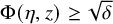 $\Phi (\eta ,z)\ge \sqrt {\delta }$
. Let
$\Phi (\eta ,z)\ge \sqrt {\delta }$
. Let
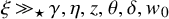 $\xi {\,\gg _{\star }\,} \gamma ,\eta ,z,\theta ,\delta ,w_0$
. Let
$\xi {\,\gg _{\star }\,} \gamma ,\eta ,z,\theta ,\delta ,w_0$
. Let
 $R\ge 2$
be an integer satisfying
$R\ge 2$
be an integer satisfying
 $\xi ^{\gamma ^{R-1}} \ge (\log \log \xi \sqrt {d})^{16d/\delta ^2}$
and
$\xi ^{\gamma ^{R-1}} \ge (\log \log \xi \sqrt {d})^{16d/\delta ^2}$
and
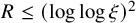 $R \le (\log \log \xi )^2$
, let
$R \le (\log \log \xi )^2$
, let
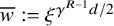 $\overline {w}:= \xi ^{\gamma ^{R-1}d/2}$
. Let
$\overline {w}:= \xi ^{\gamma ^{R-1}d/2}$
. Let
 $\mathcal {X}_{\text {high-path}}=\mathcal {X}_{\text {high-path}}(R,\eta ,y_0,y_1)$
be the event that
$\mathcal {X}_{\text {high-path}}=\mathcal {X}_{\text {high-path}}(R,\eta ,y_0,y_1)$
be the event that
 $G'$
contains a path
$G'$
contains a path
 $\pi _{y_0^\star , y_1^\star }$
fully contained in
$\pi _{y_0^\star , y_1^\star }$
fully contained in
 $\mathcal {N}$
between some vertices
$\mathcal {N}$
between some vertices
 $y^{\star }_0 \in \mathcal {N} \cap (B_{c_H\xi ^{\gamma ^{R-1}}}(y_0) \times [\overline {w}, 4\overline {w}])$
and
$y^{\star }_0 \in \mathcal {N} \cap (B_{c_H\xi ^{\gamma ^{R-1}}}(y_0) \times [\overline {w}, 4\overline {w}])$
and
 $y^{\star }_1 \in \mathcal {N} \cap (B_{c_H\xi ^{\gamma ^{R-1}}}(y_1)\times [\overline {w}, 4\overline {w}])$
with cost
$y^{\star }_1 \in \mathcal {N} \cap (B_{c_H\xi ^{\gamma ^{R-1}}}(y_1)\times [\overline {w}, 4\overline {w}])$
with cost
 $$ \begin{align} \mathcal{C}(\pi_{y_0^\star y_1^\star})\le c_H 2^R\overline{w}^{4\mu}\xi^{\eta} =c_H 2^R|x|^{2\gamma^{R-1}d\mu + \eta} \end{align} $$
and deviation
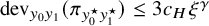 $\mathrm {dev}_{y_0y_1}(\pi _{y_0^\star y_1^\star })\le 3c_H\xi ^\gamma $
, for some constant
$\mathrm {dev}_{y_0y_1}(\pi _{y_0^\star y_1^\star })\le 3c_H\xi ^\gamma $
, for some constant
 $c_H$
depending only on
$c_H$
depending only on
 $\delta , {\texttt {par}} $
. Then
$\delta , {\texttt {par}} $
. Then
 $$ \begin{align} &\mathbb{P}\big(\mathcal{X}_{\text{high{-}path}} \mid V,w_V\big) \ge 1 - 2\exp\big({-}(\log\log\xi)^{13}\big); \end{align} $$
under the convention that
 $\infty \cdot 0 = 0$
, the statement is also valid when
$\infty \cdot 0 = 0$
, the statement is also valid when
 $\alpha =\infty $
or
$\alpha =\infty $
or
 $\beta =\infty $
.
$\beta =\infty $
.
The constant
 $c_H$
can be found below in (5.32). We postpone the proof of this proposition and show how to obtain the cost of the optimal paths from it.
$c_H$
can be found below in (5.32). We postpone the proof of this proposition and show how to obtain the cost of the optimal paths from it.
5.1 Cost optimisation of the constructed paths
In this section we apply Proposition 5.1 and optimise the cost of the path
 $\pi _{y_0^\star y_1^\star }$
constructed there, yielding either polylogarithmic (Corollary 5.2) or polynomial cost-distances (Corollary 5.3). The cost of
$\pi _{y_0^\star y_1^\star }$
constructed there, yielding either polylogarithmic (Corollary 5.2) or polynomial cost-distances (Corollary 5.3). The cost of
 $\pi _{y_0^\star y_1^\star }$
will dominate the cost of the eventual path between
$\pi _{y_0^\star y_1^\star }$
will dominate the cost of the eventual path between
 $0, x$
. These corollaries are rather immediate: we choose appropriate values of
$0, x$
. These corollaries are rather immediate: we choose appropriate values of
 $\gamma ,\eta ,z,R$
, apply Proposition 5.1, and read off the cost of
$\gamma ,\eta ,z,R$
, apply Proposition 5.1, and read off the cost of
 $\pi _{y_0^\star y_1^\star }$
in (5.2). There are four possible optimal choices of
$\pi _{y_0^\star y_1^\star }$
in (5.2). There are four possible optimal choices of
 $\gamma ,\eta , z,R$
depending on the model parameters, and verifying that the conditions of Setting 4.1 and Proposition 5.1 hold for these choices and calculating the resulting path’s cost requires some work. Thus, we defer a formal proof of Corollaries 5.2 and 5.3 to Appendix A.2, and instead focus on why these four optimisers arise and what they mean on a qualitative level.
$\gamma ,\eta , z,R$
depending on the model parameters, and verifying that the conditions of Setting 4.1 and Proposition 5.1 hold for these choices and calculating the resulting path’s cost requires some work. Thus, we defer a formal proof of Corollaries 5.2 and 5.3 to Appendix A.2, and instead focus on why these four optimisers arise and what they mean on a qualitative level.
Thus, in Proposition 5.1, disregarding constant factors, our goal is to minimise the cost bound
 $\mathcal {C}(\pi _{y_0^\star y_1^\star })\le 2^R\overline {w}^{4\mu }|x|^\eta = 2^R|x|^{2\gamma ^{R-1}d\mu + \eta }$
by choosing
$\mathcal {C}(\pi _{y_0^\star y_1^\star })\le 2^R\overline {w}^{4\mu }|x|^\eta = 2^R|x|^{2\gamma ^{R-1}d\mu + \eta }$
by choosing
 $\gamma , \eta ,z,R$
optimally. Here, R is the number of iterations in the hierarchy, and hence controls the number
$\gamma , \eta ,z,R$
optimally. Here, R is the number of iterations in the hierarchy, and hence controls the number
 $2^R$
of gaps, while
$2^R$
of gaps, while
 $\gamma $
controls the Euclidean length of the gaps and hence also the cost of joining them, with the total cost of joining a single gap being roughly
$\gamma $
controls the Euclidean length of the gaps and hence also the cost of joining them, with the total cost of joining a single gap being roughly
 $\overline {w}^{4\mu } = |x|^{2d\mu \gamma ^{R-1}}$
. The exponent
$\overline {w}^{4\mu } = |x|^{2d\mu \gamma ^{R-1}}$
. The exponent
 $\eta $
controls the cost of bridge-paths in the hierarchy. From the many constraints in Proposition 5.1, the following are relevant when optimising the cost of the path. The requirement
$\eta $
controls the cost of bridge-paths in the hierarchy. From the many constraints in Proposition 5.1, the following are relevant when optimising the cost of the path. The requirement
 $\Lambda (\eta ,z)>0$
ensures that low-cost bridging edges exist (Lemma 4.2). The requirement that either
$\Lambda (\eta ,z)>0$
ensures that low-cost bridging edges exist (Lemma 4.2). The requirement that either
 $z=0$
or
$z=0$
or
 $\Phi (\eta , z)> 0$
ensures that among the many potential bridging edges a few can be extended to low-cost 3-edge bridge-paths in Lemma 5.10. The requirement
$\Phi (\eta , z)> 0$
ensures that among the many potential bridging edges a few can be extended to low-cost 3-edge bridge-paths in Lemma 5.10. The requirement
 $\gamma <1$
ensures that boxes where we search for the bridging edge shrink in size, while
$\gamma <1$
ensures that boxes where we search for the bridging edge shrink in size, while
 $z \le d$
is a formal requirement for applying Lemma 4.2 to find bridging edges, which we tolerate because increasing z above d will never be optimal. Heuristically, the effect of increasing z is to increase the probability that a given bridging edge exists at the price of increasing its expected cost; at
$z \le d$
is a formal requirement for applying Lemma 4.2 to find bridging edges, which we tolerate because increasing z above d will never be optimal. Heuristically, the effect of increasing z is to increase the probability that a given bridging edge exists at the price of increasing its expected cost; at
 $z=d$
the existence probability is already in the interval
$z=d$
the existence probability is already in the interval
 $[\underline {c}, \overline {c}]$
and cannot be increased further, however the penalty would increase and the number of combinatorial options decrease by increasing z, which is never optimal. The other constraints of Proposition 5.1 and Setting 4.1 (such as
$[\underline {c}, \overline {c}]$
and cannot be increased further, however the penalty would increase and the number of combinatorial options decrease by increasing z, which is never optimal. The other constraints of Proposition 5.1 and Setting 4.1 (such as
 $2d\gamma < \tau -1$
and
$2d\gamma < \tau -1$
and
 $R \le (\log \log |x|)^2$
) never turn out to be tight for optimal choices of
$R \le (\log \log |x|)^2$
) never turn out to be tight for optimal choices of
 $\eta , R,\gamma , z$
. Recall
$\eta , R,\gamma , z$
. Recall
 $\mu _{\log }, \mu _{\mathrm {pol}}$
from (1.8).
$\mu _{\log }, \mu _{\mathrm {pol}}$
from (1.8).
Corollary 5.2 (Path with polylogarithmic cost).
Consider
 $1$
-FPP in Definition 1.1 on the graphs IGIRG or SFP satisfying the assumptions given in (1.6)–(1.3) with
$1$
-FPP in Definition 1.1 on the graphs IGIRG or SFP satisfying the assumptions given in (1.6)–(1.3) with
 $d\ge 1, \alpha \in (1,\infty ], \tau \in (2,3), \mu>0$
. Let
$d\ge 1, \alpha \in (1,\infty ], \tau \in (2,3), \mu>0$
. Let
 $\underline {c},\overline {c},h,L,c_1,c_2,\beta $
be as in (1.5)–(1.3), we allow
$\underline {c},\overline {c},h,L,c_1,c_2,\beta $
be as in (1.5)–(1.3), we allow
 $\beta = \infty $
and/or
$\beta = \infty $
and/or
 $\alpha =\infty $
. Let
$\alpha =\infty $
. Let
 $q,\varepsilon ,\zeta \in (0,1)$
, let
$q,\varepsilon ,\zeta \in (0,1)$
, let
 $0<\delta {\,\ll _{\star }\,} \varepsilon ,q, {\texttt {par}} $
, and let
$0<\delta {\,\ll _{\star }\,} \varepsilon ,q, {\texttt {par}} $
, and let
 $w_0>1$
. Fix a realisation
$w_0>1$
. Fix a realisation
 $(V, w_V)$
of
$(V, w_V)$
of
 $\widetilde {\cal V}$
. Let
$\widetilde {\cal V}$
. Let
 $x \in V$
with
$x \in V$
with
 $|x|{\,\gg _{\star }\,} q, \delta ,\varepsilon ,\zeta , w_0, {\texttt {par}} $
. Let Q be a cube of side length
$|x|{\,\gg _{\star }\,} q, \delta ,\varepsilon ,\zeta , w_0, {\texttt {par}} $
. Let Q be a cube of side length
 $|x|$
containing
$|x|$
containing
 $0$
and x, and assume that
$0$
and x, and assume that
 $(V, w_V)$
is such that Q contains a weak
$(V, w_V)$
is such that Q contains a weak
 $(\delta /4,w_0)$
-net
$(\delta /4,w_0)$
-net
 $\mathcal {N}$
with
$\mathcal {N}$
with
 $0,x \in \mathcal {N}$
given in Definition 2.1. Let
$0,x \in \mathcal {N}$
given in Definition 2.1. Let
 $G \sim \{\mathcal {G}\mid V, w_V\}$
. Let
$G \sim \{\mathcal {G}\mid V, w_V\}$
. Let
 $\mathcal {X}_{\mathrm {polylog}}(0,x)$
be the event that G contains a path
$\mathcal {X}_{\mathrm {polylog}}(0,x)$
be the event that G contains a path
 $\pi $
, fully contained in
$\pi $
, fully contained in
 $\mathcal {N}$
, with endpoints say
$\mathcal {N}$
, with endpoints say
 $y_0^\star , y_x^\star $
, with the following properties:
$y_0^\star , y_x^\star $
, with the following properties:
 $$ \begin{align} &w_{y_0^\star}, w_{y_x^\star} \in [\overline{w},4\overline{w}], \quad \text{where} \quad \overline{w} \in [\log\log|x|, (\log|x|)^\varepsilon], \end{align} $$
 $$ \begin{align} &y_0^\star \in B_{\overline{w}^{3/d}}(0) \qquad\qquad \text{and} \qquad y_x^\star \in B_{\overline{w}^{3/d}}(x) , \end{align} $$
 $$ \begin{align} &\mathcal{C}(\pi) \le (\log |x|)^{\Delta_0+\varepsilon}, \qquad \text{and} \qquad \mathrm{dev}_{0x}(\pi)\le \zeta |x|, \end{align} $$
where
 $\Delta _0$
is defined in (1.9), (1.17) or (1.20) depending on whether
$\Delta _0$
is defined in (1.9), (1.17) or (1.20) depending on whether
 $\alpha ,\beta <\infty $
,
$\alpha ,\beta <\infty $
,
 $\alpha =\infty $
or
$\alpha =\infty $
or
 $\beta =\infty $
. If either
$\beta =\infty $
. If either
 $\alpha \in (1,2)$
or
$\alpha \in (1,2)$
or
 $\mu \in (\mu _{\mathrm {expl}},\mu _{\log })$
or both hold, then
$\mu \in (\mu _{\mathrm {expl}},\mu _{\log })$
or both hold, then
 $\mathbb {P}(\mathcal {X}_{\mathrm {polylog}}(0,x) \mid V,w_V) \ge 1-q$
.
$\mathbb {P}(\mathcal {X}_{\mathrm {polylog}}(0,x) \mid V,w_V) \ge 1-q$
.
Sketch of proof.
Corollary 5.2 covers the polylogarithmic regime, which corresponds to solutions where
 $\eta = 0$
is possible – such solutions exists when either
$\eta = 0$
is possible – such solutions exists when either
 $\alpha \in (1,2)$
or
$\alpha \in (1,2)$
or
 $\mu <\mu _{\log }$
. When
$\mu <\mu _{\log }$
. When
 $\eta =0$
, the cost of the path
$\eta =0$
, the cost of the path
 $\pi _{y_0^\star ,y_x^\star }$
is dominated by the cost
$\pi _{y_0^\star ,y_x^\star }$
is dominated by the cost
 $2^R|x|^{2\mu \gamma ^{R-1}}$
of joining gaps. Given
$2^R|x|^{2\mu \gamma ^{R-1}}$
of joining gaps. Given
 $\gamma $
, this has minimum
$\gamma $
, this has minimum
 $2^{(1+o(1))R}$
when setting
$2^{(1+o(1))R}$
when setting
 $R = (1-o(1))\log \log |x|/\log (1/\gamma )$
. To minimise the cost further, we must therefore minimise
$R = (1-o(1))\log \log |x|/\log (1/\gamma )$
. To minimise the cost further, we must therefore minimise
 $\gamma \in (0,1)$
subject to the constraints
$\gamma \in (0,1)$
subject to the constraints
 $z\in [0,d], \Lambda (0,z)>0$
, and either
$z\in [0,d], \Lambda (0,z)>0$
, and either
 $z=0$
or
$z=0$
or
 $\Phi (0,z)>0$
. This problem turns out to have two potentially optimal solutions corresponding to two possible strategies for finding bridging edges, with the optimal choice depending on the values of
$\Phi (0,z)>0$
. This problem turns out to have two potentially optimal solutions corresponding to two possible strategies for finding bridging edges, with the optimal choice depending on the values of
 $\alpha ,\tau ,\beta ,\mu $
. One possible solution – which only exists when
$\alpha ,\tau ,\beta ,\mu $
. One possible solution – which only exists when
 $\alpha \in (1,2)$
– takes
$\alpha \in (1,2)$
– takes
 $\gamma = \alpha /2 + o(1)$
and
$\gamma = \alpha /2 + o(1)$
and
 $z=0$
, so that bridging edges are unusually long-range edges between pairs of low-weight vertices, yielding total path cost
$z=0$
, so that bridging edges are unusually long-range edges between pairs of low-weight vertices, yielding total path cost
 $(\log |x|)^{\Delta _\alpha }$
with
$(\log |x|)^{\Delta _\alpha }$
with
 $\Delta _\alpha =1/(1-\log _2\alpha )$
, see Claim A.5. The other possible solution – which only exists when
$\Delta _\alpha =1/(1-\log _2\alpha )$
, see Claim A.5. The other possible solution – which only exists when
 $\mu <\mu _{\log }$
– takes
$\mu <\mu _{\log }$
– takes
 $\gamma = (\tau -1+\mu \beta )/2 + o(1)$
and
$\gamma = (\tau -1+\mu \beta )/2 + o(1)$
and
 $z=d$
, so that bridging edges are unusually low-cost edges between pairs of high-weight vertices and the total path cost is
$z=d$
, so that bridging edges are unusually low-cost edges between pairs of high-weight vertices and the total path cost is
 $(\log x)^{\Delta _\beta }$
with
$(\log x)^{\Delta _\beta }$
with
 $\Delta _\beta =1/(1-\log _2(\tau -1+\mu \beta ))$
, see Claim A.6. The proof is in Appendix A.2.
$\Delta _\beta =1/(1-\log _2(\tau -1+\mu \beta ))$
, see Claim A.6. The proof is in Appendix A.2.
If both
 $\alpha =\beta =\infty $
, then the conditions of Corollary 5.2 cannot be satisfied. Indeed, when
$\alpha =\beta =\infty $
, then the conditions of Corollary 5.2 cannot be satisfied. Indeed, when
 $\alpha =\infty $
then
$\alpha =\infty $
then
 $\alpha \in (1,2)$
is not satisfied. Since
$\alpha \in (1,2)$
is not satisfied. Since
 $\mu _{\mathrm {expl}}= \mu _{\log } = 0$
by (1.19) when
$\mu _{\mathrm {expl}}= \mu _{\log } = 0$
by (1.19) when
 $\alpha =\beta =\infty $
, so
$\alpha =\beta =\infty $
, so
 $\mu \in (\mu _{\mathrm {expl}},\mu _{\log })$
can also not be satisfied.
$\mu \in (\mu _{\mathrm {expl}},\mu _{\log })$
can also not be satisfied.
Corollary 5.3 (Path with polynomial cost).
Consider
 $1$
-FPP in Definition 1.1 on the graphs IGIRG or SFP satisfying the assumptions given in (1.6)–(1.3) with
$1$
-FPP in Definition 1.1 on the graphs IGIRG or SFP satisfying the assumptions given in (1.6)–(1.3) with
 $d\ge 1, \alpha \in (1,\infty ], \tau \in (2,3), \mu>0$
. Let
$d\ge 1, \alpha \in (1,\infty ], \tau \in (2,3), \mu>0$
. Let
 $\underline {c},\overline {c},h,L,c_1,c_2,\beta $
be as in (1.5)–(1.3), we allow
$\underline {c},\overline {c},h,L,c_1,c_2,\beta $
be as in (1.5)–(1.3), we allow
 $\beta = \infty $
and/or
$\beta = \infty $
and/or
 $\alpha =\infty $
. Let
$\alpha =\infty $
. Let
 $q,\varepsilon ,\zeta \in (0,1)$
, and let
$q,\varepsilon ,\zeta \in (0,1)$
, and let
 $0<\delta {\,\ll _{\star }\,} \varepsilon ,q, {\texttt {par}} $
, and
$0<\delta {\,\ll _{\star }\,} \varepsilon ,q, {\texttt {par}} $
, and
 $w_0>1$
. Fix a realisation
$w_0>1$
. Fix a realisation
 $(V, w_V)$
of
$(V, w_V)$
of
 $\widetilde {\cal V}$
. Let
$\widetilde {\cal V}$
. Let
 $x \in V$
with
$x \in V$
with
 $|x|{\,\gg _{\star }\,} q,\delta ,\varepsilon , \zeta ,w_0, {\texttt {par}} $
. Let Q be a cube of side length
$|x|{\,\gg _{\star }\,} q,\delta ,\varepsilon , \zeta ,w_0, {\texttt {par}} $
. Let Q be a cube of side length
 $|x|$
containing
$|x|$
containing
 $0$
and x, and assume that
$0$
and x, and assume that
 $(V, w_V)$
is such that Q contains a weak
$(V, w_V)$
is such that Q contains a weak
 $(\delta /4,w_0)$
-net
$(\delta /4,w_0)$
-net
 $\mathcal {N}$
with
$\mathcal {N}$
with
 $0,x \in \mathcal {N}$
given in Definition 2.1. Let
$0,x \in \mathcal {N}$
given in Definition 2.1. Let
 $G \sim \{\mathcal {G}\mid V, w_V\}$
. Let
$G \sim \{\mathcal {G}\mid V, w_V\}$
. Let
 $\mathcal {X}_{\mathrm {pol}}(0,x)$
be the event that G contains a path
$\mathcal {X}_{\mathrm {pol}}(0,x)$
be the event that G contains a path
 $\pi $
, fully contained in
$\pi $
, fully contained in
 $\mathcal {N}$
, with endpoints say
$\mathcal {N}$
, with endpoints say
 $y_0^\star , y_x^\star $
, with the following properties:
$y_0^\star , y_x^\star $
, with the following properties:
 $$ \begin{align} &w_{y_0^\star}, w_{y_x^\star} \in [\overline{w},4\overline{w}], \quad \text{where} \quad \overline{w} \in [\log\log|x|, |x|^\varepsilon], \end{align} $$
 $$ \begin{align} &y_0^\star \in B_{\overline{w}^{3/d}}(0) \qquad\qquad \text{and} \qquad y_x^\star \in B_{\overline{w}^{3/d}}(x) , \end{align} $$
 $$ \begin{align} &\mathcal{C}(\pi) \le |x|^{\eta_0+\varepsilon}, \qquad \text{and} \qquad \mathrm{dev}_{0x}(\pi)\le \zeta |x|, \end{align} $$
where
 $\eta _0$
is defined in (1.10), (1.16), (1.19), or (1.21) depending on
$\eta _0$
is defined in (1.10), (1.16), (1.19), or (1.21) depending on
 $\alpha ,\beta <\infty $
,
$\alpha ,\beta <\infty $
,
 $\alpha =\infty $
,
$\alpha =\infty $
,
 $\beta =\infty $
, or
$\beta =\infty $
, or
 $\alpha =\beta =\infty $
. If both
$\alpha =\beta =\infty $
. If both
 $\alpha>2$
and
$\alpha>2$
and
 $\mu \in (\mu _{\log }, \mu _{\mathrm {pol}}]$
hold then
$\mu \in (\mu _{\log }, \mu _{\mathrm {pol}}]$
hold then
 $\mathbb {P}(\mathcal {X}_{\mathrm {pol}}(0,x) \mid V,w_V) \ge 1-q$
.
$\mathbb {P}(\mathcal {X}_{\mathrm {pol}}(0,x) \mid V,w_V) \ge 1-q$
.
Sketch of proof.
Corollary 5.3 covers the polynomial regime, which corresponds to solutions where only
 $\eta> 0$
is possible, that is, when
$\eta> 0$
is possible, that is, when
 $\alpha>2$
and
$\alpha>2$
and
 $\mu>\mu _{\log }$
. Here, on taking R to be a suitably large constant, the cost bound on the path
$\mu>\mu _{\log }$
. Here, on taking R to be a suitably large constant, the cost bound on the path
 $2^R|x|^{2\mu \gamma ^{R-1}}|x|^\eta =|x|^{\eta +o(1)}$
, which is roughly the cost of the very first bridging edge. Our goal is thus to minimise
$2^R|x|^{2\mu \gamma ^{R-1}}|x|^\eta =|x|^{\eta +o(1)}$
, which is roughly the cost of the very first bridging edge. Our goal is thus to minimise
 $\eta $
under the constraints that
$\eta $
under the constraints that
 $\Lambda (\eta ,z)>0$
,
$\Lambda (\eta ,z)>0$
,
 $z\in [0,d]$
,
$z\in [0,d]$
,
 $\gamma \in (0,1)$
, and either
$\gamma \in (0,1)$
, and either
 $z=0$
or
$z=0$
or
 $\Phi (\eta ,z)>0$
. (4.1) and (5.1) show that both
$\Phi (\eta ,z)>0$
. (4.1) and (5.1) show that both
 $\Phi $
and
$\Phi $
and
 $\Lambda $
are increasing functions of
$\Lambda $
are increasing functions of
 $\gamma $
; thus we can take
$\gamma $
; thus we can take
 $\gamma = 1-o(1)$
. As in the polylogarithmic regime, this minimisation problem has two potentially optimal solutions. One possible solution – which exists when
$\gamma = 1-o(1)$
. As in the polylogarithmic regime, this minimisation problem has two potentially optimal solutions. One possible solution – which exists when
 $\mu \le \mu _{\mathrm {pol},\beta }$
– takes
$\mu \le \mu _{\mathrm {pol},\beta }$
– takes
 $z=d$
and gives
$z=d$
and gives
 $\eta = \mu d-(3-\tau )d/\beta + o(1)$
, so that bridging edges are unusually low-cost edges between pairs of high-weight vertices. The total path cost is then
$\eta = \mu d-(3-\tau )d/\beta + o(1)$
, so that bridging edges are unusually low-cost edges between pairs of high-weight vertices. The total path cost is then
 $|x|^{\eta _\beta +o(1)}$
with
$|x|^{\eta _\beta +o(1)}$
with
 $\eta _\beta =d(\mu -(3-\tau )/\beta )$
(see Claim A.9). The other possible solution – which exists when
$\eta _\beta =d(\mu -(3-\tau )/\beta )$
(see Claim A.9). The other possible solution – which exists when
 $\mu \le \mu _{\mathrm {pol},\alpha }$
– takes z to be as small as possible, so that bridging edges are unusually long-range edges between pairs of relatively low-weight vertices. However, when
$\mu \le \mu _{\mathrm {pol},\alpha }$
– takes z to be as small as possible, so that bridging edges are unusually long-range edges between pairs of relatively low-weight vertices. However, when
 $\alpha>2$
, there are no bridging-edges between constant weight vertices, and the minimal z where bridging-edges appear is
$\alpha>2$
, there are no bridging-edges between constant weight vertices, and the minimal z where bridging-edges appear is
 $z = d(\alpha -2)/(\alpha - (\tau - 1)) + o(1)=1/\mu _{\mathrm {pol},\alpha }+o(1)$
, that is, between vertices of weight
$z = d(\alpha -2)/(\alpha - (\tau - 1)) + o(1)=1/\mu _{\mathrm {pol},\alpha }+o(1)$
, that is, between vertices of weight
 $|x|^{1/(2\mu _{\mathrm {pol},\alpha })+o(1)}$
. This gives cost-exponent
$|x|^{1/(2\mu _{\mathrm {pol},\alpha })+o(1)}$
. This gives cost-exponent
 $\eta _\alpha := \mu /\mu _{\mathrm {pol},\alpha }$
and total cost
$\eta _\alpha := \mu /\mu _{\mathrm {pol},\alpha }$
and total cost
 $|x|^{\mu /\mu _{\mathrm {pol},\alpha } + o(1)}$
(see Claim A.10). Whenever a solution exists among the above two possibilities, it gives an exponent
$|x|^{\mu /\mu _{\mathrm {pol},\alpha } + o(1)}$
(see Claim A.10). Whenever a solution exists among the above two possibilities, it gives an exponent
 $\eta $
at most
$\eta $
at most
 $1$
. So, whenever
$1$
. So, whenever
 $\mu \le \max \{\mu _{\mathrm {pol},\alpha }, \mu _{\mathrm {pol},\beta }\}$
, we obtain the cost bound
$\mu \le \max \{\mu _{\mathrm {pol},\alpha }, \mu _{\mathrm {pol},\beta }\}$
, we obtain the cost bound
 $|x|^{\min \{\eta _\beta , \eta _\alpha \}+o(1)}$
, which gives the definition of
$|x|^{\min \{\eta _\beta , \eta _\alpha \}+o(1)}$
, which gives the definition of
 $\eta _0$
in (1.10). The proof is in Appendix A.2.
$\eta _0$
in (1.10). The proof is in Appendix A.2.
5.2 Constructing the hierarchy.
We now set out to prove Proposition 5.1 in several steps. We start by formally defining the concept of a hierarchy including edge-costs. In the rest of the paper, the symbol
 $\sigma $
denotes an index
$\sigma $
denotes an index
 $\sigma =\sigma _1\sigma _2\ldots \sigma _R\in \{0,1\}^R$
indicating the place of a vertex in the hierarchy. This can be viewed as the Ulam-Harris labelling of the leaves of a binary tree of depth R, for example,
$\sigma =\sigma _1\sigma _2\ldots \sigma _R\in \{0,1\}^R$
indicating the place of a vertex in the hierarchy. This can be viewed as the Ulam-Harris labelling of the leaves of a binary tree of depth R, for example,
 $\sigma = 1001$
corresponds to the leaf that we reach by starting at the root and then moving to the right child, the left child twice, and the right child again. We denote the string formed by concatenating
$\sigma = 1001$
corresponds to the leaf that we reach by starting at the root and then moving to the right child, the left child twice, and the right child again. We denote the string formed by concatenating
 $\sigma '$
to the end of
$\sigma '$
to the end of
 $\sigma $
by
$\sigma $
by
 $\sigma \sigma '$
. We ‘pad’ strings of length less than R by adding copies of their last digit or its complement via the T and
$\sigma \sigma '$
. We ‘pad’ strings of length less than R by adding copies of their last digit or its complement via the T and
 $T^c$
operations we now define (and discuss further below):
$T^c$
operations we now define (and discuss further below):
Definition 5.4 (Binary strings).
For
 $\sigma =\sigma _1\ldots \sigma _i\in \{0,1\}^i$
for some
$\sigma =\sigma _1\ldots \sigma _i\in \{0,1\}^i$
for some
 $i\ge 1$
, we define
$i\ge 1$
, we define
 $\sigma T:=\sigma _1\ldots \sigma _i\sigma _i\in \{0,1\}^{i+1}$
, while
$\sigma T:=\sigma _1\ldots \sigma _i\sigma _i\in \{0,1\}^{i+1}$
, while
 $\sigma T_0:=\sigma $
, and
$\sigma T_0:=\sigma $
, and
 $\sigma T_k:=(\sigma T_{k-1})T$
for any
$\sigma T_k:=(\sigma T_{k-1})T$
for any
 $k\ge 2$
. Let
$k\ge 2$
. Let
 $0_i:=0T_{i-1}$
and
$0_i:=0T_{i-1}$
and
 $1_i:=1T_{i-1}$
be the strings consisting of i copies of
$1_i:=1T_{i-1}$
be the strings consisting of i copies of
 $0$
and
$0$
and
 $1$
, respectively. Fix an integer
$1$
, respectively. Fix an integer
 $R \ge 1$
. Define the equivalence relation
$R \ge 1$
. Define the equivalence relation
 $\sim _T$
on
$\sim _T$
on
 $\cup _{i=1}^R\{0,1\}^i$
, where
$\cup _{i=1}^R\{0,1\}^i$
, where
 $\sigma \sim _T \sigma '$
if either
$\sigma \sim _T \sigma '$
if either
 $\sigma T_k=\sigma '$
or
$\sigma T_k=\sigma '$
or
 $\sigma 'T_k=\sigma $
for some
$\sigma 'T_k=\sigma $
for some
 $k\ge 0$
, with
$k\ge 0$
, with
 $\{\sigma \}$
be the equivalence class of
$\{\sigma \}$
be the equivalence class of
 $\sigma $
. Let
$\sigma $
. Let
 $$ \begin{align*} \Xi_{i}:=\{ \sigma \in \cup_{j=i}^R\{0,1\}^j: \sigma_{i-1} \neq \sigma_i, \sigma_{j}=\sigma_i \ \forall j\ge i\}, \qquad \Xi_0:=\{\emptyset\}, \end{align*} $$
with
 $\emptyset $
the empty string. We say that
$\emptyset $
the empty string. We say that
 $\{\sigma \}$
appears first on level i if any (the shortest) representative of the class
$\{\sigma \}$
appears first on level i if any (the shortest) representative of the class
 $\{\sigma \}$
is contained in
$\{\sigma \}$
is contained in
 $\Xi _i$
.
$\Xi _i$
.
For
 $\sigma =\sigma _1\ldots \sigma _i\in \{0,1\}^i$
for some
$\sigma =\sigma _1\ldots \sigma _i\in \{0,1\}^i$
for some
 $i\ge 1$
, we define
$i\ge 1$
, we define
 $\sigma T^c:=\sigma _1\ldots \sigma _i(1-\sigma _i)\in \{0,1\}^{i+1}$
. For
$\sigma T^c:=\sigma _1\ldots \sigma _i(1-\sigma _i)\in \{0,1\}^{i+1}$
. For
 $\sigma \in \Xi _i$
, we say that
$\sigma \in \Xi _i$
, we say that
 $(\sigma T_{j-1})T^c\in \{0,1\}^{i+j}$
is the level-(i+j) sibling of
$(\sigma T_{j-1})T^c\in \{0,1\}^{i+j}$
is the level-(i+j) sibling of
 $\{\sigma \}$
. We say that two strings in level i are newly appearing cousins on level i if they are of the forms
$\{\sigma \}$
. We say that two strings in level i are newly appearing cousins on level i if they are of the forms
 $\sigma 01$
and
$\sigma 01$
and
 $\sigma 10$
for some
$\sigma 10$
for some
 $\sigma \in \{0,1\}^{i-2}$
.
$\sigma \in \{0,1\}^{i-2}$
.
The inverse of the operator T ‘cuts off’ all but one of the identical last digits from a
 $\sigma \in \{0,1\}^R$
, hence, each class
$\sigma \in \{0,1\}^R$
, hence, each class
 $\{\sigma \}$
has exactly one representative in
$\{\sigma \}$
has exactly one representative in
 $\{0,1\}^R$
, and the number of equivalence classes is
$\{0,1\}^R$
, and the number of equivalence classes is
 $2^R$
. For
$2^R$
. For
 $i>1$
, there are exactly
$i>1$
, there are exactly
 $2^{i-1}$
equivalence classes that first appear on level i (i.e., the shortest representative of the class is in
$2^{i-1}$
equivalence classes that first appear on level i (i.e., the shortest representative of the class is in
 $\Xi _i$
), and (since
$\Xi _i$
), and (since
 $0, 1\in \Xi _1$
) the total number of equivalence classes that appear until level i is
$0, 1\in \Xi _1$
) the total number of equivalence classes that appear until level i is
 $2^i$
. To show an example of the sibling relationship, for example,
$2^i$
. To show an example of the sibling relationship, for example,
 $01111\sim 01$
belongs to
$01111\sim 01$
belongs to
 $\Xi _2$
, and the level-
$\Xi _2$
, and the level-
 $3$
sibling of
$3$
sibling of
 $\{01\}$
is
$\{01\}$
is
 $010$
, and the level-
$010$
, and the level-
 $(2+j)$
sibling of
$(2+j)$
sibling of
 $\{01\}$
is
$\{01\}$
is
 $01_j0$
. Similarly,
$01_j0$
. Similarly,
 $010$
and
$010$
and
 $001$
are newly appearing level-
$001$
are newly appearing level-
 $3$
cousins, and on level i, there are
$3$
cousins, and on level i, there are
 $2^{i-2}$
pairs of newly appearing cousins.
$2^{i-2}$
pairs of newly appearing cousins.
The hierarchy embeds each equivalence class
 $\{\sigma \}\in \cup _{j=1}^{R}\{0,1\}^R$
into the (weighted) vertex set of G so that all cousins are joined by low-cost ‘bridge’ paths, all siblings are close in Euclidean space,
$\{\sigma \}\in \cup _{j=1}^{R}\{0,1\}^R$
into the (weighted) vertex set of G so that all cousins are joined by low-cost ‘bridge’ paths, all siblings are close in Euclidean space,
 $0^R=x$
and
$0^R=x$
and
 $1^R=y$
are the vertices we start with, and the weights of all other vertices in the embedding are constrained. The Euclidean distances between siblings/cousins will decay doubly exponentially in i. We formalise the embedding in the following definition.
$1^R=y$
are the vertices we start with, and the weights of all other vertices in the embedding are constrained. The Euclidean distances between siblings/cousins will decay doubly exponentially in i. We formalise the embedding in the following definition.
Definition 5.5 (Hierarchy).
Consider Setting 4.1. Let
 $y_0, y_1 \in \widetilde {\mathcal {V}}$
,
$y_0, y_1 \in \widetilde {\mathcal {V}}$
,
 $U,\overline {w},c_H\ge 1$
, and
$U,\overline {w},c_H\ge 1$
, and
 $R\ge 2$
be an integer. Consider a set of vertices
$R\ge 2$
be an integer. Consider a set of vertices
 $\{y_{\sigma }\}_{\sigma \in \{0,1\}^R}$
, divided into levels
$\{y_{\sigma }\}_{\sigma \in \{0,1\}^R}$
, divided into levels
 ${\mathcal {L}}_i:=\{y_{\sigma } \colon \sigma \in \Xi _i\}$
for
${\mathcal {L}}_i:=\{y_{\sigma } \colon \sigma \in \Xi _i\}$
for
 $i\in \{1,\ldots ,R\}$
, satisfying that
$i\in \{1,\ldots ,R\}$
, satisfying that
 $y_{\sigma }=y_{\sigma '}$
if
$y_{\sigma }=y_{\sigma '}$
if
 $\sigma \sim _T \sigma '$
. We say that
$\sigma \sim _T \sigma '$
. We say that
 $\{y_{\sigma }\}_{\sigma \in \{0,1\}^R}\subset \widetilde {\mathcal {V}}$
is a
$\{y_{\sigma }\}_{\sigma \in \{0,1\}^R}\subset \widetilde {\mathcal {V}}$
is a
 $(\gamma , U, \overline {w}, c_H)$
-hierarchy of depth R with
$(\gamma , U, \overline {w}, c_H)$
-hierarchy of depth R with
 $\mathcal {L}_1=\{y_0, y_1\}$
if it satisfies the following properties:
$\mathcal {L}_1=\{y_0, y_1\}$
if it satisfies the following properties:
-
(H1)
$W_{y_{\sigma }}\in [\overline {w}, 4\overline {w}]$
for all
$\sigma \in \{0,1\}^R \setminus \Xi _1$
. -
(H2)
$|y_{\sigma 0}-y_{\sigma 1}|\le c_H|y_0-y_1|^{\gamma ^i}$
for all
$\sigma \in \{0,1\}^i$
,
$i=0,\ldots ,R-1$
. -
(H3) There is a set
$\{P_{\sigma } : \sigma \in \{0,1\}^i, 0\le i \le R-2\}$
of paths in G such that for all
$0 \le i \le R-2$
and all
$\sigma \in \{0,1\}^i$
,
$P_{\sigma }$
connects
$y_{\sigma 01}$
to
$y_{\sigma 10}$
. Moreover, we can partition
$\bigcup _{\sigma \in \{0,1\}^R} \mathcal {E}(P_\sigma )$
into sets
$\{\mathcal {E}^-(P_\sigma )\colon \sigma \in \{0,1\}^R\}$
in such a way that for all
$\sigma $
, we have
$\mathcal {E}^-(P_\sigma ) \subseteq \mathcal {E}(P_\sigma )$
and
$\mathcal {C}(\mathcal {E}^-(P_\sigma )) \le U$
. These paths
$P_{\sigma }$
are called bridges.


Given a set
 $\mathcal {N} \subseteq \widetilde {\mathcal {V}}$
, we say that a hierarchy
$\mathcal {N} \subseteq \widetilde {\mathcal {V}}$
, we say that a hierarchy
 $\{y_\sigma \}_{\sigma \in \{0,1\}^R}$
is fully contained in
$\{y_\sigma \}_{\sigma \in \{0,1\}^R}$
is fully contained in
 $\mathcal {N}$
if both
$\mathcal {N}$
if both
 $\{y_\sigma \}_{\sigma \in \{0,1\}^R} \subseteq \mathcal {N}$
, and every vertex on the paths
$\{y_\sigma \}_{\sigma \in \{0,1\}^R} \subseteq \mathcal {N}$
, and every vertex on the paths
 $P_{\sigma }$
in (H3) lies in
$P_{\sigma }$
in (H3) lies in
 $\mathcal {N}$
.
$\mathcal {N}$
.
Condition (H3) is slightly weaker than requiring each bridge to have cost at most U. We shall construct the hierarchy via an iterative construction in Def. 3.6, using one round to embed each level
 $\mathcal {L}_i$
. We shall use Prop. 3.9 to estimate the success probability of the whole construction, which requires that we use marginal costs, and this gives the definition of
$\mathcal {L}_i$
. We shall use Prop. 3.9 to estimate the success probability of the whole construction, which requires that we use marginal costs, and this gives the definition of
 $\mathcal {E}^-(P_\sigma )$
in (3.1). Using marginal costs causes no problem, since our goal is to find a path
$\mathcal {E}^-(P_\sigma )$
in (3.1). Using marginal costs causes no problem, since our goal is to find a path
 $\pi $
between
$\pi $
between
 $y_0$
and
$y_0$
and
 $y_1$
of low cost. A path
$y_1$
of low cost. A path
 $\pi $
uses every edge in it once, so all the bridges
$\pi $
uses every edge in it once, so all the bridges
 $P_\sigma $
together will contribute to the cost of
$P_\sigma $
together will contribute to the cost of
 $\pi $
at most
$\pi $
at most
 $$ \begin{align*} \mathcal{C}(\pi) = \sum_{\sigma\in\{0,1\}^i, 0\le i \le R-2} \mathcal{C}(\mathcal{E}^-(P_\sigma)) \le (2^{R-1}-1) U. \end{align*} $$
Later we also need that the the hierarchy stays close to the straight line segment between the starting vertices. To track this, we have the following definition:
Definition 5.6. Given
 $u,v \in \mathbb {R}^d$
, let
$u,v \in \mathbb {R}^d$
, let
 $S_{u,v}$
denote the line segment between
$S_{u,v}$
denote the line segment between
 $u,v$
. For
$u,v$
. For
 $x\in \mathbb {R}^d$
we define the deviation
$x\in \mathbb {R}^d$
we define the deviation
 $\mathrm {dev}_{uv}(x):=\min \{|x-y|: y\in S_{u,v}\}$
. Given a set of vertices
$\mathrm {dev}_{uv}(x):=\min \{|x-y|: y\in S_{u,v}\}$
. Given a set of vertices
 $\mathcal {H}$
in
$\mathcal {H}$
in
 $\mathbb {R}^d$
, we define the deviation of
$\mathbb {R}^d$
, we define the deviation of
 $\mathcal {H}$
from
$\mathcal {H}$
from
 $S_{uv}$
as
$S_{uv}$
as
 $\mathrm {dev}_{uv}(\mathcal {H}):=\max \{\mathrm {dev}_{uv}(x) \colon x\in \mathcal {H} \}$
. Finally, for a path
$\mathrm {dev}_{uv}(\mathcal {H}):=\max \{\mathrm {dev}_{uv}(x) \colon x\in \mathcal {H} \}$
. Finally, for a path
 $\pi =(x_1\dots x_k)$
, let the deviation of
$\pi =(x_1\dots x_k)$
, let the deviation of
 $\pi $
be
$\pi $
be
 $\mathrm {dev}(\pi ) := \max \{\mathrm {dev}_{x_1x_k}(x_i) \colon i \in [k]\}$
, that is, the deviation of its vertex set from the segment between the endpoints.
$\mathrm {dev}(\pi ) := \max \{\mathrm {dev}_{x_1x_k}(x_i) \colon i \in [k]\}$
, that is, the deviation of its vertex set from the segment between the endpoints.
Next we describe the procedure used to find the hierarchy in G. We iteratively embed the levels
 $\Xi _i$
into the vertex set
$\Xi _i$
into the vertex set
 $\widetilde {\mathcal {V}}$
. We first embed
$\widetilde {\mathcal {V}}$
. We first embed
 $\Xi _1$
, by setting
$\Xi _1$
, by setting
 $0\mapsto y_0$
and
$0\mapsto y_0$
and
 $1\mapsto y_1$
, that is,
$1\mapsto y_1$
, that is,
 $\mathcal {L}_1:=\{y_0, y_1\}$
, the two given starting vertices. Observe that this embedding trivially satisfies condition (H2) for
$\mathcal {L}_1:=\{y_0, y_1\}$
, the two given starting vertices. Observe that this embedding trivially satisfies condition (H2) for
 $i=0$
, (i.e.,
$i=0$
, (i.e.,
 $\sigma =\emptyset $
in (H2)) for all
$\sigma =\emptyset $
in (H2)) for all
 $c_H\ge 1$
. Conditions (H1) and (H3) do not concern
$c_H\ge 1$
. Conditions (H1) and (H3) do not concern
 $y_0$
and
$y_0$
and
 $y_1$
. In round
$y_1$
. In round
 $i+1$
we then embed all
$i+1$
we then embed all
 $\sigma \in \Xi _{i+1}$
. Given the embedding of
$\sigma \in \Xi _{i+1}$
. Given the embedding of
 $\cup _{j\le i}\Xi _j$
of vertices in level
$\cup _{j\le i}\Xi _j$
of vertices in level
 $\cup _{j\le i}\mathcal {L}_j$
, we will embed
$\cup _{j\le i}\mathcal {L}_j$
, we will embed
 $\sigma \in \Xi _{i+1} $
by finding
$\sigma \in \Xi _{i+1} $
by finding
 $\{y_{\sigma }\}_{\sigma \in \Xi _{i+1}}=\mathcal {L}_{i+1}$
as follows. For each sibling pair
$\{y_{\sigma }\}_{\sigma \in \Xi _{i+1}}=\mathcal {L}_{i+1}$
as follows. For each sibling pair
 $\sigma 0, \sigma 1 \in \{0,1\}^i$
, by the equivalence relation
$\sigma 0, \sigma 1 \in \{0,1\}^i$
, by the equivalence relation
 $\sim _T$
in Definition 5.4,
$\sim _T$
in Definition 5.4,
 $y_{\sigma 00} = y_{\sigma 0}$
and
$y_{\sigma 00} = y_{\sigma 0}$
and
 $y_{\sigma 11} = y_{\sigma 1}$
. We then search for a pair of vertices a and b close to
$y_{\sigma 11} = y_{\sigma 1}$
. We then search for a pair of vertices a and b close to
 $y_{\sigma 00}$
and
$y_{\sigma 00}$
and
 $y_{\sigma 11}$
respectively, so that
$y_{\sigma 11}$
respectively, so that
 $ab$
is a low-cost edge (typically covering a large Euclidean distance), and both a and b have a low-cost edge to a nearby vertex with weight in
$ab$
is a low-cost edge (typically covering a large Euclidean distance), and both a and b have a low-cost edge to a nearby vertex with weight in
 $[\overline {w},4\overline {w}]$
; we embed these latter two vertices as
$[\overline {w},4\overline {w}]$
; we embed these latter two vertices as
 $y_{\sigma 01}$
and
$y_{\sigma 01}$
and
 $y_{\sigma 10}$
. The path
$y_{\sigma 10}$
. The path
 $(y_{\sigma 01}aby_{\sigma 10})$
then constitutes the bridge-path
$(y_{\sigma 01}aby_{\sigma 10})$
then constitutes the bridge-path
 $P_{\sigma }$
required by (H3). See Figure 5 for a visual explanation. We formalise our goal for this iterative construction of bridges in the following definition and lemma.
$P_{\sigma }$
required by (H3). See Figure 5 for a visual explanation. We formalise our goal for this iterative construction of bridges in the following definition and lemma.
A schematic representation of a
 $(\gamma , U, \overline {w}, 2)$
-hierarchy of depth
$(\gamma , U, \overline {w}, 2)$
-hierarchy of depth
 $R\!=\!3$
. The horizontal axis represents the (
$R\!=\!3$
. The horizontal axis represents the (
 $1$
-dimensional, Euclidean) distances between the vertices, while the vertical axis shows the level of the hierarchy. The weights of all vertices except
$1$
-dimensional, Euclidean) distances between the vertices, while the vertical axis shows the level of the hierarchy. The weights of all vertices except
 $y_0$
and
$y_0$
and
 $y_1$
are in the interval
$y_1$
are in the interval
 $[\overline {w}, 4\overline {w}]$
. On level
$[\overline {w}, 4\overline {w}]$
. On level
 $1$
, only the initial vertices
$1$
, only the initial vertices
 $y_0, y_1$
appear and n edges. We ‘push down’
$y_0, y_1$
appear and n edges. We ‘push down’
 $y_0=y_{00}, y_{1}=y_{11}$
to level
$y_0=y_{00}, y_{1}=y_{11}$
to level
 $2$
(red) and we find them their respective level-
$2$
(red) and we find them their respective level-
 $2$
sibling vertices
$2$
sibling vertices
 $y_{01}$
and
$y_{01}$
and
 $y_{10}$
within Euclidean distance
$y_{10}$
within Euclidean distance
 $2\xi ^\gamma $
, so that there is path of cost at most U between
$2\xi ^\gamma $
, so that there is path of cost at most U between
 $y_{01}, y_{10}$
(represented by the longest blue arc). Then, we ‘push down’ to level
$y_{01}, y_{10}$
(represented by the longest blue arc). Then, we ‘push down’ to level
 $3$
all vertices that appeared at or before level
$3$
all vertices that appeared at or before level
 $2$
, that is,
$2$
, that is,
 $y_{000}, y_{011}, y_{100}, y_{111}$
(red), and find for each of them their level-
$y_{000}, y_{011}, y_{100}, y_{111}$
(red), and find for each of them their level-
 $3$
siblings, that is,
$3$
siblings, that is,
 $y_{001}, y_{010}, y_{101}, y_{110}$
, so that each vertex is within Euclidean distance
$y_{001}, y_{010}, y_{101}, y_{110}$
, so that each vertex is within Euclidean distance
 $\le 2 \xi ^{\gamma ^2}$
from its level-
$\le 2 \xi ^{\gamma ^2}$
from its level-
 $3$
sibling, and that there is a path of cost at most U between the newly appearing cousins
$3$
sibling, and that there is a path of cost at most U between the newly appearing cousins
 $y_{001}, y_{010}$
and between
$y_{001}, y_{010}$
and between
 $y_{101}, y_{110}$
(represented by the two shrter blue arcs). An intuitive representation is in Figure 2.
$y_{101}, y_{110}$
(represented by the two shrter blue arcs). An intuitive representation is in Figure 2.

Definition 5.7 (Valid bridges).
Consider Setting 4.1 and the notion of bridges in Definition 5.5, and let S be a set of edges of G. For any
 $D,U>0, w\ge 1$
, we say that a path
$D,U>0, w\ge 1$
, we say that a path
 $P \subseteq \mathcal {N}$
with endpoints
$P \subseteq \mathcal {N}$
with endpoints
 $y,y'$
is a
$y,y'$
is a
 $(D,U,w)$
-valid bridge for
$(D,U,w)$
-valid bridge for
 $x_0$
and
$x_0$
and
 $x_1$
with respect to S if:
$x_1$
with respect to S if:
 $$ \begin{align} &w_y, w_{y'} \in [w,4w], \end{align} $$
 $$ \begin{align} &|x_0-y|\le D, \quad \text{and}\quad |x_1-y'| \le D, \end{align} $$
 $$ \begin{align} & \mathcal{C}(P\setminus S)\le U. \end{align} $$
Lemma 5.8. Consider Setting 4.1. Fix any ordering on
 $\{0,1\}^R$
, and let
$\{0,1\}^R$
, and let
 $\{y_\sigma \}_{\sigma \in \{0,1\}^R} \subseteq \mathcal {N}$
,
$\{y_\sigma \}_{\sigma \in \{0,1\}^R} \subseteq \mathcal {N}$
,
 $U> 0$
, and
$U> 0$
, and
 $\overline {w} \ge 1$
. For all
$\overline {w} \ge 1$
. For all
 $0 \le i \le R-2$
and
$0 \le i \le R-2$
and
 $\sigma \in \{0,1\}^i$
, set
$\sigma \in \{0,1\}^i$
, set
 $y_{\sigma '} := y_\sigma $
whenever
$y_{\sigma '} := y_\sigma $
whenever
 $\sigma '\sim _T\sigma $
. For all
$\sigma '\sim _T\sigma $
. For all
 $i \le R-2$
, let
$i \le R-2$
, let
 $D_{i} =|y_0-y_1|^{\gamma ^{i}}$
. Suppose that for all
$D_{i} =|y_0-y_1|^{\gamma ^{i}}$
. Suppose that for all
 $0 \le i \le R-2$
and all
$0 \le i \le R-2$
and all
 $\sigma \in \{0,1\}^i$
, there exists a bridge
$\sigma \in \{0,1\}^i$
, there exists a bridge
 $P_{\sigma }$
with endpoints
$P_{\sigma }$
with endpoints
 $y_{\sigma 01}$
and
$y_{\sigma 01}$
and
 $y_{\sigma 10}$
that is
$y_{\sigma 10}$
that is
 $(c_HD_{i+1}, U, \overline {w})$
-valid for
$(c_HD_{i+1}, U, \overline {w})$
-valid for
 $y_{\sigma 0},y_{\sigma 1} \in \{0,1\}^{i+1}$
with respect to
$y_{\sigma 0},y_{\sigma 1} \in \{0,1\}^{i+1}$
with respect to
 $S=\bigcup _{\sigma ' < \sigma }\mathcal {E}(P_{\sigma '})$
. Then
$S=\bigcup _{\sigma ' < \sigma }\mathcal {E}(P_{\sigma '})$
. Then
 $\{y_\sigma \}_{\sigma \in \{0,1\}^R}$
is a
$\{y_\sigma \}_{\sigma \in \{0,1\}^R}$
is a
 $(\gamma ,U,\overline {w}, c_H)$
-hierarchy of depth R with first level
$(\gamma ,U,\overline {w}, c_H)$
-hierarchy of depth R with first level
 $\{y_0,y_1\}$
(i.e., satisfying Definition 5.5).
$\{y_0,y_1\}$
(i.e., satisfying Definition 5.5).
Proof. Conditions (H1) of Definition 5.5 is immediate from the weight constraint (5.10). (H2) holds for the following reason. For
 $\sigma 0, \sigma 1 \in \{0,1\}^{i+1}$
,
$\sigma 0, \sigma 1 \in \{0,1\}^{i+1}$
,
 $P_\sigma $
being a
$P_\sigma $
being a
 $(c_HD_{i+1}, U, \overline {w})$
valid bridge for
$(c_HD_{i+1}, U, \overline {w})$
valid bridge for
 $y_{\sigma 0}, y_{\sigma 1}$
implies by (5.11) and
$y_{\sigma 0}, y_{\sigma 1}$
implies by (5.11) and
 $y_{\sigma 0}=y_{\sigma 00}, y_{\sigma 1}=y_{\sigma 11}$
that both
$y_{\sigma 0}=y_{\sigma 00}, y_{\sigma 1}=y_{\sigma 11}$
that both
 $|y_{\sigma 00}- y_{\sigma 01}|, |y_{\sigma 10}- y_{\sigma 11}|$
are at most
$|y_{\sigma 00}- y_{\sigma 01}|, |y_{\sigma 10}- y_{\sigma 11}|$
are at most
 $c_H|y_0-y_1|^{\gamma ^{i+1}}$
for all
$c_H|y_0-y_1|^{\gamma ^{i+1}}$
for all
 $\sigma \in \{0,1\}^i$
. Setting now either
$\sigma \in \{0,1\}^i$
. Setting now either
 $\sigma ':=\sigma 0$
or
$\sigma ':=\sigma 0$
or
 $\sigma ':=\sigma 1$
, this is equivalent to
$\sigma ':=\sigma 1$
, this is equivalent to
 $|y_{\sigma '0}-y_{\sigma '1}|\le c_H|y_0-y_1|^{\gamma ^{i+1}}$
for all
$|y_{\sigma '0}-y_{\sigma '1}|\le c_H|y_0-y_1|^{\gamma ^{i+1}}$
for all
 $\sigma '\in \{0,1\}^{i+1}, i\ge 0$
, and this exactly corresponds to (H2), since the inequality in (H2) holds for
$\sigma '\in \{0,1\}^{i+1}, i\ge 0$
, and this exactly corresponds to (H2), since the inequality in (H2) holds for
 $i=0$
trivially. Finally, condition (H3) follows from (5.12) by setting
$i=0$
trivially. Finally, condition (H3) follows from (5.12) by setting
 $\mathcal {E}^-(P_{\sigma }) := \mathcal {E}(P_\sigma ) \setminus \bigcup _{\sigma ' < \sigma }\mathcal {E}(P_{\sigma '})$
.
$\mathcal {E}^-(P_{\sigma }) := \mathcal {E}(P_\sigma ) \setminus \bigcup _{\sigma ' < \sigma }\mathcal {E}(P_{\sigma '})$
.
We now lower-bound the probability of finding a valid bridge between two fixed vertices. Recall that
 $G'$
is a
$G'$
is a
 $\theta $
-percolation of G from Setting 4.1.
$\theta $
-percolation of G from Setting 4.1.
Lemma 5.9 (3-edge bridges).
Consider Setting 4.1. Let
 $z \in [0,d]$
and let
$z \in [0,d]$
and let
 $c_H,\eta \ge 0$
. Suppose that
$c_H,\eta \ge 0$
. Suppose that
 $\delta {\,\ll _{\star }\,} \gamma ,\eta ,z,c_H, {\texttt {par}} $
and that
$\delta {\,\ll _{\star }\,} \gamma ,\eta ,z,c_H, {\texttt {par}} $
and that
 $D{\,\gg _{\star }\,} \gamma ,\eta ,z,c_H,\delta ,w_0$
. Suppose further that
$D{\,\gg _{\star }\,} \gamma ,\eta ,z,c_H,\delta ,w_0$
. Suppose further that
 $D^\gamma \in [4^{1/d}(\log \log \xi \sqrt {d})^{16/\delta }, \xi \sqrt {d} ]$
and that
$D^\gamma \in [4^{1/d}(\log \log \xi \sqrt {d})^{16/\delta }, \xi \sqrt {d} ]$
and that
 $\theta D^{\Lambda (\eta ,z)-\sqrt {\delta }}> 1$
. Suppose that
$\theta D^{\Lambda (\eta ,z)-\sqrt {\delta }}> 1$
. Suppose that
 $x_0, x_1 \in \mathcal {N}$
satisfy
$x_0, x_1 \in \mathcal {N}$
satisfy
 $|x_0-x_1| \le c_HD$
, and let
$|x_0-x_1| \le c_HD$
, and let
 $\underline {w} {\,\gg _{\star }\,} \delta ,w_0$
satisfy
$\underline {w} {\,\gg _{\star }\,} \delta ,w_0$
satisfy
 $\underline {w}\in [(\log \log \xi \sqrt {d})^{16d/\delta }, D^{\delta }]$
. Let
$\underline {w}\in [(\log \log \xi \sqrt {d})^{16d/\delta }, D^{\delta }]$
. Let
 $\mathcal {A}(x_0,x_1)$
denote the event that
$\mathcal {A}(x_0,x_1)$
denote the event that
 $G'$
contains a bridge P that is
$G'$
contains a bridge P that is
 $(2D^\gamma ,3\underline {w}^{3\mu }D^{\eta },\underline {w})$
-valid for
$(2D^\gamma ,3\underline {w}^{3\mu }D^{\eta },\underline {w})$
-valid for
 $x_0$
and
$x_0$
and
 $x_1$
with respect to
$x_1$
with respect to
 $\emptyset $
, and
$\emptyset $
, and
 $\mathrm {dev}_{x_0x_1}(P)\le 2D^\gamma $
. Finally, suppose that
$\mathrm {dev}_{x_0x_1}(P)\le 2D^\gamma $
. Finally, suppose that
 $$ \begin{align} p(D, \underline{w}, \theta, \eta, z):= \theta \underline{w}^{-(\tau-1)}\left(D^{d\gamma} \wedge \underline{w}^2 D^{z/2}\right)^{1-\delta}\left(1 \wedge \underline{w}^{\mu\beta}D^{\eta\beta-\mu\beta z/2}\right) \ge 20^{\tau+\mu\beta}. \end{align} $$
Then, with
 $\Lambda (\eta ,z)$
from (4.1),
$\Lambda (\eta ,z)$
from (4.1),
 $$ \begin{align} \mathbb{P}\big(\mathcal{A}(x_0,x_1) \mid V,w_V\big) \ge 1 - 3\exp\left(-\big(\theta D^{\Lambda(\eta,z)-\sqrt{\delta}}\big)^{1/4}\right). \end{align} $$
With the convention that
 $\infty \cdot 0 = 0$
in (4.1), the statement is also valid when
$\infty \cdot 0 = 0$
in (4.1), the statement is also valid when
 $\alpha =\infty $
or
$\alpha =\infty $
or
 $\beta =\infty $
.
$\beta =\infty $
.
When
 $z>0$
, the exponent of D in
$z>0$
, the exponent of D in
 $p(\cdot )$
is approximating
$p(\cdot )$
is approximating
 $\Phi (\eta ,z)$
for small
$\Phi (\eta ,z)$
for small
 $\delta $
in (5.1). Later,
$\delta $
in (5.1). Later,
 $\Phi (\eta , z)>\sqrt {\delta }$
will be sufficient for the condition (5.13) to hold when
$\Phi (\eta , z)>\sqrt {\delta }$
will be sufficient for the condition (5.13) to hold when
 $z>0$
. For
$z>0$
. For
 $z=0$
, D does not appear in the formula for
$z=0$
, D does not appear in the formula for
 $p(\cdot )$
, and the exponent of
$p(\cdot )$
, and the exponent of
 $\underline {w}$
is approximating
$\underline {w}$
is approximating
 $3-\tau>0$
, hence in this case the condition on
$3-\tau>0$
, hence in this case the condition on
 $p(\cdot )$
can be satisfied by ensuring the lower bound on
$p(\cdot )$
can be satisfied by ensuring the lower bound on
 $\underline {w}$
.
$\underline {w}$
.
Proof of Lemma 5.9.
First, when
 $\beta =\infty $
and
$\beta =\infty $
and
 $\eta < \mu z$
then
$\eta < \mu z$
then
 $\Lambda (\eta ,z)=-\infty $
in (4.1), and the condition
$\Lambda (\eta ,z)=-\infty $
in (4.1), and the condition
 $\theta D^{\Lambda (\eta ,z)-\sqrt {\delta }}> 1$
cannot hold. Hence, we can wlog assume that if
$\theta D^{\Lambda (\eta ,z)-\sqrt {\delta }}> 1$
cannot hold. Hence, we can wlog assume that if
 $\beta =\infty $
then
$\beta =\infty $
then
 $\eta \ge \mu z$
. We will first apply Lemma 4.3 to show that most vertices of weight roughly
$\eta \ge \mu z$
. We will first apply Lemma 4.3 to show that most vertices of weight roughly
 $\underline {w} D^{z/2}$
close to
$\underline {w} D^{z/2}$
close to
 $x_0$
and
$x_0$
and
 $x_1$
are ‘good’, that is, they have a cheap edge to a vertex with weight in
$x_1$
are ‘good’, that is, they have a cheap edge to a vertex with weight in
 $[\underline {w},4\underline {w}]$
. We will then apply Lemma 4.2 to find a cheap edge between some pair of good vertices.
$[\underline {w},4\underline {w}]$
. We will then apply Lemma 4.2 to find a cheap edge between some pair of good vertices.
Formally, let
 $I^+ = [5\underline {w} D^{z/2}, 20\underline {w} D^{z/2}]$
and
$I^+ = [5\underline {w} D^{z/2}, 20\underline {w} D^{z/2}]$
and
 $I^- = [\underline {w}, 4\underline {w}]$
. Note that
$I^- = [\underline {w}, 4\underline {w}]$
. Note that
 $I_+\cap I_-=\emptyset $
for all
$I_+\cap I_-=\emptyset $
for all
 $z\in [0,d]$
. As in Lemma 4.3, for all
$z\in [0,d]$
. As in Lemma 4.3, for all
 $v \in \mathcal {N}$
let
$v \in \mathcal {N}$
let
 $\mathcal {A}_{2\underline {w},D^\gamma ,\underline {w}^{3\mu }D^{\eta }}(v)=:\mathcal {A}(v)$
be the event that there is an edge of cost at most
$\mathcal {A}_{2\underline {w},D^\gamma ,\underline {w}^{3\mu }D^{\eta }}(v)=:\mathcal {A}(v)$
be the event that there is an edge of cost at most
 $\underline {w}^{3\mu }D^{\eta }$
in
$\underline {w}^{3\mu }D^{\eta }$
in
 $G'$
from v to a vertex
$G'$
from v to a vertex
 $y \in \mathcal {N} \cap (B_{D^\gamma }(v) \times I^-)$
. Let
$y \in \mathcal {N} \cap (B_{D^\gamma }(v) \times I^-)$
. Let
 $$ \begin{align} Z_i := \big\{v \in \mathcal{N} \cap (B_{D^\gamma}(x_i) \times I^+) \colon \mathcal{A}(v)\text{ occurs}\big\}, \qquad i \in \{0,1\}. \end{align} $$
The set
 $Z_i$
is thus those high weight vertices near
$Z_i$
is thus those high weight vertices near
 $x_i$
that have a cheap edge to a low-weight vertex nearby. As in (4.3) of Lemma 4.2, let
$x_i$
that have a cheap edge to a low-weight vertex nearby. As in (4.3) of Lemma 4.2, let
 $N_{\eta ,\gamma ,z,10\underline {w}}(Z_0,Z_1)$
be the set of all edges between
$N_{\eta ,\gamma ,z,10\underline {w}}(Z_0,Z_1)$
be the set of all edges between
 $Z_0$
and
$Z_0$
and
 $Z_1$
of cost at most
$Z_1$
of cost at most
 $\underline {w}^{3\mu }D^\eta $
and then
$\underline {w}^{3\mu }D^\eta $
and then
 $I^+$
exactly corresponds to the weight interval
$I^+$
exactly corresponds to the weight interval
 $[5\underline {w} D^{z/2}, 20\underline {w} D^{z/2}]$
as required for
$[5\underline {w} D^{z/2}, 20\underline {w} D^{z/2}]$
as required for
 $Z_0\subseteq \mathcal {Z}(x_0), Z_1\subseteq \mathcal {Z}(x_1)$
in (4.2). With
$Z_0\subseteq \mathcal {Z}(x_0), Z_1\subseteq \mathcal {Z}(x_1)$
in (4.2). With
 $Z_i$
in (5.15), we now show that
$Z_i$
in (5.15), we now show that
 $$ \begin{align} \mathbb{P}\big(\mathcal{A}(x_0,x_1) \mid V,w_V\big) \ge \mathbb{P}\big(N_{\eta,\gamma,z,\underline{w}}(Z_0,Z_1) \ne \emptyset \mid V,w_V\big). \end{align} $$
Indeed, suppose there exists
 $(a,b) \in N_{\eta ,\gamma ,z,10\underline {w}}(Z_0,Z_1)$
. Since
$(a,b) \in N_{\eta ,\gamma ,z,10\underline {w}}(Z_0,Z_1)$
. Since
 $a \in Z_0$
, there exists
$a \in Z_0$
, there exists
 $x \in \mathcal {N} \cap (B_{D^\gamma }(a)\times I^-)$
such that
$x \in \mathcal {N} \cap (B_{D^\gamma }(a)\times I^-)$
such that
 $(x,a)$
is an edge of cost at most
$(x,a)$
is an edge of cost at most
 $\underline {w}^{3\mu }D^\eta $
. Likewise, since
$\underline {w}^{3\mu }D^\eta $
. Likewise, since
 $b \in Z_1$
, there exists
$b \in Z_1$
, there exists
 $y \in \mathcal {N} \cap (B_{D^\gamma }(b) \times I^-)$
such that
$y \in \mathcal {N} \cap (B_{D^\gamma }(b) \times I^-)$
such that
 $(y,b)$
is an edge of cost at most
$(y,b)$
is an edge of cost at most
 $\underline {w}^{3\mu }D^\eta $
. Since
$\underline {w}^{3\mu }D^\eta $
. Since
 $a \in B_{D^\gamma }(x_0)$
and
$a \in B_{D^\gamma }(x_0)$
and
 $b \in B_{D^\gamma }(x_1)$
, by the triangle inequality,
$b \in B_{D^\gamma }(x_1)$
, by the triangle inequality,
 $x \in B_{2D^\gamma }(x_0)$
and
$x \in B_{2D^\gamma }(x_0)$
and
 $y \in B_{2D^\gamma }(x_1)$
. Thus
$y \in B_{2D^\gamma }(x_1)$
. Thus
 $xaby$
is a
$xaby$
is a
 $(2D^\gamma , 3\underline {w}^{3\mu }D^\eta , \underline {w})$
-valid bridge with
$(2D^\gamma , 3\underline {w}^{3\mu }D^\eta , \underline {w})$
-valid bridge with
 $\mathrm {dev}_{x_0x_1}\le 2D^\gamma $
, as required by
$\mathrm {dev}_{x_0x_1}\le 2D^\gamma $
, as required by
 $\mathcal {A}(x_0,x_1)$
, showing (5.16).
$\mathcal {A}(x_0,x_1)$
, showing (5.16).
Now, for each
 $i \in \{0,1\}$
, using (4.2), we set
$i \in \{0,1\}$
, using (4.2), we set
 $\mathcal {Z}(x_i) = \mathcal {N} \cap (B_{D^\gamma }(x_i) \times I^+)$
. For (4.4) to hold we need that
$\mathcal {Z}(x_i) = \mathcal {N} \cap (B_{D^\gamma }(x_i) \times I^+)$
. For (4.4) to hold we need that
 $|Z_i| \ge |\mathcal {Z}(x_i)|/4$
. We prove this by showing that any given vertex in
$|Z_i| \ge |\mathcal {Z}(x_i)|/4$
. We prove this by showing that any given vertex in
 $v \in \mathcal {Z}(x_i)$
lies in
$v \in \mathcal {Z}(x_i)$
lies in
 $Z_i$
with probability at least
$Z_i$
with probability at least
 $1/2$
, by recalling that in (5.15),
$1/2$
, by recalling that in (5.15),
 $\mathcal {A}(v)=\mathcal {A}_{2\underline {w},D^\gamma ,\underline {w}^{3\mu }D^{\eta }}(v)=\mathcal {A}_{K,D,U}(v)$
in Lemma 4.3. Hence we set
$\mathcal {A}(v)=\mathcal {A}_{2\underline {w},D^\gamma ,\underline {w}^{3\mu }D^{\eta }}(v)=\mathcal {A}_{K,D,U}(v)$
in Lemma 4.3. Hence we set
 $K = 2\underline {w}, M = 10\underline {w} D^{z/2}, U = \underline {w}^{3\mu }D^{\eta }$
,
$K = 2\underline {w}, M = 10\underline {w} D^{z/2}, U = \underline {w}^{3\mu }D^{\eta }$
,
 $D_{{\scriptstyle 4.3}}=D^\gamma $
, and all other variables to match their current values. We check the requirements of Lemma 4.3:
$D_{{\scriptstyle 4.3}}=D^\gamma $
, and all other variables to match their current values. We check the requirements of Lemma 4.3:
By hypothesis in the statement of Lemma 5.9,
 $\delta $
is small;
$\delta $
is small;
 $\underline {w},D{\,\gg _{\star }\,} \delta ,w_0$
, and
$\underline {w},D{\,\gg _{\star }\,} \delta ,w_0$
, and
 $D{\,\gg _{\star }\,} \gamma $
. Since
$D{\,\gg _{\star }\,} \gamma $
. Since
 $M,K \ge \underline {w}$
, it follows that
$M,K \ge \underline {w}$
, it follows that
 $M,K,D^\gamma {\,\gg _{\star }\,} \delta , w_0$
, as required above (4.11). Condition (4.11) itself holds since
$M,K,D^\gamma {\,\gg _{\star }\,} \delta , w_0$
, as required above (4.11). Condition (4.11) itself holds since
 $(D^\gamma \wedge (20\underline {w}^2 D^{z/2})^{1/d}/4^{1/d} \ge D^\gamma /4^{1/d} \wedge \underline {w}^{1/d} \ge (\log \log \xi \sqrt {d})^{16/\delta }$
by hypothesis, and
$(D^\gamma \wedge (20\underline {w}^2 D^{z/2})^{1/d}/4^{1/d} \ge D^\gamma /4^{1/d} \wedge \underline {w}^{1/d} \ge (\log \log \xi \sqrt {d})^{16/\delta }$
by hypothesis, and
 $(D^\gamma \wedge (20\underline {w}^2 D^{z/2})^{1/d}/4^{1/d} \le D^\gamma \le \xi \sqrt {d}$
by hypothesis. Condition (4.12) holds since
$(D^\gamma \wedge (20\underline {w}^2 D^{z/2})^{1/d}/4^{1/d} \le D^\gamma \le \xi \sqrt {d}$
by hypothesis. Condition (4.12) holds since
 $K=2\underline {w} \le 2D^{\delta }$
by hypothesis, so since
$K=2\underline {w} \le 2D^{\delta }$
by hypothesis, so since
 $\delta {\,\ll _{\star }\,} \gamma $
and
$\delta {\,\ll _{\star }\,} \gamma $
and
 $D{\,\gg _{\star }\,}\delta $
, we have
$D{\,\gg _{\star }\,}\delta $
, we have
 $2\underline {w} \le D^{\gamma (d/(\tau -1)-\delta )}$
, and similarly since
$2\underline {w} \le D^{\gamma (d/(\tau -1)-\delta )}$
, and similarly since
 $\tau \in (2,3)$
and
$\tau \in (2,3)$
and
 $\delta {\,\ll _{\star }\,} {\texttt {par}} $
,
$\delta {\,\ll _{\star }\,} {\texttt {par}} $
,
 $K=2\underline {w} \le (2\underline {w})^{1/(\tau -2+\tau \delta )} \le (10\underline {w} D^{z/2})^{1/(\tau -2+\delta \tau )}=M^{1/(\tau -2+\delta \tau )}$
. Finally, if
$K=2\underline {w} \le (2\underline {w})^{1/(\tau -2+\tau \delta )} \le (10\underline {w} D^{z/2})^{1/(\tau -2+\delta \tau )}=M^{1/(\tau -2+\delta \tau )}$
. Finally, if
 $\beta =\infty $
, then below (4.12) we need to check
$\beta =\infty $
, then below (4.12) we need to check
 $U(KM)^{-\mu }{\,\gg _{\star }\,} {\texttt {par}} $
. Since wlog we assumed that
$U(KM)^{-\mu }{\,\gg _{\star }\,} {\texttt {par}} $
. Since wlog we assumed that
 $\eta \ge \mu z$
, clearly
$\eta \ge \mu z$
, clearly
 $\eta \ge \mu z/2$
. Therefore,
$\eta \ge \mu z/2$
. Therefore,
 $U(KM)^{-\mu }=\underline {w}^{3\mu }D^{\eta }(20\underline {w}^2 D^{z/2})^{-\mu } = 20^{-\mu }\underline {w}^{\mu }D^{\eta -\mu z/2} \ge (\underline {w}/20)^{\mu }$
, which is large since
$U(KM)^{-\mu }=\underline {w}^{3\mu }D^{\eta }(20\underline {w}^2 D^{z/2})^{-\mu } = 20^{-\mu }\underline {w}^{\mu }D^{\eta -\mu z/2} \ge (\underline {w}/20)^{\mu }$
, which is large since
 $\underline {w}$
is large by hypothesis. Hence, all conditions of Lemma 4.3 are met and (4.13) applies, and substituting
$\underline {w}$
is large by hypothesis. Hence, all conditions of Lemma 4.3 are met and (4.13) applies, and substituting
 $K = 2\underline {w}, M = 10\underline {w} D^{z/2}, U = \underline {w}^{3\mu }D^{\eta }$
there, the exponent on the right-hand side of (4.13) in our setting becomes
$K = 2\underline {w}, M = 10\underline {w} D^{z/2}, U = \underline {w}^{3\mu }D^{\eta }$
there, the exponent on the right-hand side of (4.13) in our setting becomes
 $$\begin{align*}-2^{-(\tau-1)} \theta \underline{w}^{-(\tau-1)}\big(D^{d\gamma} \wedge 20\underline{w}^2D^{z/2}\big)^{1-\delta}\left(1 \wedge (\underline{w}/20)^{\mu\beta}D^{\eta\beta-\mu\beta z/2}\right), \end{align*}$$
where we recognise that this matches
 $p(\cdot )$
from (5.13) up to a factor of at most
$p(\cdot )$
from (5.13) up to a factor of at most
 $20^{1-(\tau +\mu \beta )}$
. Since we assumed
$20^{1-(\tau +\mu \beta )}$
. Since we assumed
 $p(\cdot )\ge 20^{\tau +\mu \beta }$
in (5.13), for any vertex
$p(\cdot )\ge 20^{\tau +\mu \beta }$
in (5.13), for any vertex
 $v \in \mathcal {Z}(x_i)=\mathcal {N} \cap (B_{D^\gamma }(x_i) \times I^+)$
,
$v \in \mathcal {Z}(x_i)=\mathcal {N} \cap (B_{D^\gamma }(x_i) \times I^+)$
,
 $$ \begin{align} \mathbb{P}\big(v \in Z_i \mid V,w_V\big) = \mathbb{P}(\mathcal{A}(v) \mid V, w_V) \ge 1 - e^{-20}> 1/2. \end{align} $$
Since
 $I^+$
and
$I^+$
and
 $I^-$
are disjoint, the events
$I^-$
are disjoint, the events
 $\mathcal {A}(v), \mathcal {A}(v')$
are functions of disjoint edge sets and are therefore mutually independent conditioned on
$\mathcal {A}(v), \mathcal {A}(v')$
are functions of disjoint edge sets and are therefore mutually independent conditioned on
 $(V, w_V)$
. Hence, for
$(V, w_V)$
. Hence, for
 $i \in \{0,1\}$
,
$i \in \{0,1\}$
,
 $|Z_i|$
is dominated below by a binomial variable with mean
$|Z_i|$
is dominated below by a binomial variable with mean
 $|\mathcal {Z}(x_i)|/2$
. By the standard Chernoff bound (Theorem A.1 with
$|\mathcal {Z}(x_i)|/2$
. By the standard Chernoff bound (Theorem A.1 with
 $\lambda =1/2$
),
$\lambda =1/2$
),
$$ \begin{align} \mathbb{P}\big(|Z_i| < |\mathcal{Z}(x_i)|/4 \mid V,w_V\big) \le e^{-|\mathcal{Z}(x_i)|/16}. \end{align} $$
To bound
 $|\mathcal {Z}(x_i)|$
below in (5.18), we will use that
$|\mathcal {Z}(x_i)|$
below in (5.18), we will use that
 $x_0,x_1 \in \mathcal {N}$
and
$x_0,x_1 \in \mathcal {N}$
and
 $\mathcal {N}$
is a weak
$\mathcal {N}$
is a weak
 $(\delta /4,w_0)$
-net as assumed in Setting 4.1, and apply (2.2). We check if the conditions to apply (2.2) in Def. 2.1 hold. Since
$(\delta /4,w_0)$
-net as assumed in Setting 4.1, and apply (2.2). We check if the conditions to apply (2.2) in Def. 2.1 hold. Since
 $\mathcal {Z}(x_i)=\mathcal {N} \cap (B_{D^\gamma }(x_i) \times [5\underline {w} D^{z/2}, 20\underline {w} D^{z/2}])$
, we set there
$\mathcal {Z}(x_i)=\mathcal {N} \cap (B_{D^\gamma }(x_i) \times [5\underline {w} D^{z/2}, 20\underline {w} D^{z/2}])$
, we set there
 $r=D^\gamma $
and
$r=D^\gamma $
and
 $w=10\underline {w} D^{z/2}$
, and we must bound
$w=10\underline {w} D^{z/2}$
, and we must bound
 $10\underline {w} D^{z/2}$
above and below. Recall that by hypothesis,
$10\underline {w} D^{z/2}$
above and below. Recall that by hypothesis,
 $\theta D^{\Lambda (\eta ,z)-\sqrt {\delta }}> 1$
; this implies
$\theta D^{\Lambda (\eta ,z)-\sqrt {\delta }}> 1$
; this implies
 $\Lambda (\eta ,z)> 0$
and hence
$\Lambda (\eta ,z)> 0$
and hence
 $2d\gamma> z(\tau -1)$
using (4.1). Since
$2d\gamma> z(\tau -1)$
using (4.1). Since
 $\delta {\,\ll _{\star }\,} \gamma ,z$
, we may therefore assume
$\delta {\,\ll _{\star }\,} \gamma ,z$
, we may therefore assume
 $z/2 \le d\gamma /(\tau -1) - 2\delta $
. Also, we assumed
$z/2 \le d\gamma /(\tau -1) - 2\delta $
. Also, we assumed
 $\underline {w} \le D^\delta $
, so
$\underline {w} \le D^\delta $
, so
 $10\underline {w} D^{z/2} \le 10D^{d\gamma /(\tau -1)-\delta } \le (D^{\gamma })^{d/(\tau -1)-\delta /4}$
, where the second inequality holds since
$10\underline {w} D^{z/2} \le 10D^{d\gamma /(\tau -1)-\delta } \le (D^{\gamma })^{d/(\tau -1)-\delta /4}$
, where the second inequality holds since
 $\gamma <1$
and
$\gamma <1$
and
 $D{\,\gg _{\star }\,} \delta $
. Moreover, since
$D{\,\gg _{\star }\,} \delta $
. Moreover, since
 $\underline {w}{\,\gg _{\star }\,} w_0$
, we have
$\underline {w}{\,\gg _{\star }\,} w_0$
, we have
 $10\underline {w} D^{z/2} \ge w_0$
. Thus all conditions in Def. 2.1 are met, and (2.2) here becomes
$10\underline {w} D^{z/2} \ge w_0$
. Thus all conditions in Def. 2.1 are met, and (2.2) here becomes
 $$\begin{align*}|\mathcal{Z}(x_i)| \ge D^{d\gamma(1-\delta/4)}\ell(10\underline{w} D^{z/2})(10\underline{w} D^{z/2})^{-(\tau-1)}\ge D^{d\gamma(1-\delta/4) - (\tau-1+\delta/4)(\delta + z/2)}, \end{align*}$$
where the second inequality holds by Potter’s bound since
 $D^{\delta } \ge \underline {w}\gg \delta $
. The exponent of D on the right-hand side is
$D^{\delta } \ge \underline {w}\gg \delta $
. The exponent of D on the right-hand side is
 $$\begin{align*}d\gamma-(\tau-1)z/2-\delta(d\gamma/4+z/8+\tau-1+\delta/4) \ge d\gamma/2-(\tau-1)z/2 \ge \Lambda(\eta,z)/4, \end{align*}$$
where we used
 $\delta {\,\ll _{\star }\,} \gamma $
and then the formula of
$\delta {\,\ll _{\star }\,} \gamma $
and then the formula of
 $\Lambda (\eta ,z)$
in (4.1). So,
$\Lambda (\eta ,z)$
in (4.1). So,
 $|\mathcal {Z}(x_i)| \ge D^{\Lambda (\eta ,z)/4}$
in (5.18), and since
$|\mathcal {Z}(x_i)| \ge D^{\Lambda (\eta ,z)/4}$
in (5.18), and since
 $D{\,\gg _{\star }\,} \delta $
,
$D{\,\gg _{\star }\,} \delta $
,
$$ \begin{align} \mathbb{P}\big(|Z_i| < |\mathcal{Z}(x_i)|/4 \mid V,w_V\big) \le \exp(-D^{\Lambda(\eta,z)/4}/16)\le \exp(-(\theta D^{\Lambda(\eta,z) - \sqrt{\delta}})^{1/4}). \end{align} $$
Returning to the event
 $\mathcal {A}(x_0, x_1)$
in (5.16), let
$\mathcal {A}(x_0, x_1)$
in (5.16), let
 $\mathcal {A}'$
be the event that
$\mathcal {A}'$
be the event that
 $|Z_i| \ge |\mathcal {Z}(x_i)|/4$
for each
$|Z_i| \ge |\mathcal {Z}(x_i)|/4$
for each
 $i \in \{0,1\}$
, and suppose that
$i \in \{0,1\}$
, and suppose that
 $\mathcal {A}'$
occurs. Observe also that the set
$\mathcal {A}'$
occurs. Observe also that the set
 $Z_i\subseteq \mathcal {Z}(x_i)$
were chosen independently of the edges between
$Z_i\subseteq \mathcal {Z}(x_i)$
were chosen independently of the edges between
 $\mathcal {Z}(x_0), \mathcal {Z}(x_1)$
as required in Lemma 4.2. We apply Lemma 4.2, conditioned on the values of
$\mathcal {Z}(x_0), \mathcal {Z}(x_1)$
as required in Lemma 4.2. We apply Lemma 4.2, conditioned on the values of
 $Z_0$
and
$Z_0$
and
 $Z_1$
, to lower-bound the right-hand side of (5.16). In the statement of Lemma 4.2, we will take
$Z_1$
, to lower-bound the right-hand side of (5.16). In the statement of Lemma 4.2, we will take
 $x = x_0$
,
$x = x_0$
,
 $y = x_1$
,
$y = x_1$
,
 $Z_x = Z_0$
,
$Z_x = Z_0$
,
 $Z_y = Z_1$
,
$Z_y = Z_1$
,
 $\underline {w}_{4.2} = 10\underline {w}$
, and all other variables to match their current values. The event
$\underline {w}_{4.2} = 10\underline {w}$
, and all other variables to match their current values. The event
 $N_{\eta ,\gamma ,z,10\underline {w}}(Z_0,Z_1) \ne \emptyset $
of (5.16) requires a low-cost edge between the set
$N_{\eta ,\gamma ,z,10\underline {w}}(Z_0,Z_1) \ne \emptyset $
of (5.16) requires a low-cost edge between the set
 $Z_0$
and
$Z_0$
and
 $Z_1$
, connecting vertices with weights in
$Z_1$
, connecting vertices with weights in
 $I_+$
. Given
$I_+$
. Given
 $(V, w_V)$
, the existence of such an edge
$(V, w_V)$
, the existence of such an edge
 $(u,v)$
is independent of the events
$(u,v)$
is independent of the events
 $\mathcal {A}(u), \mathcal {A}(v)$
since in
$\mathcal {A}(u), \mathcal {A}(v)$
since in
 $\mathcal {A}(\cdot )$
the other endpoint of the edge has weight
$\mathcal {A}(\cdot )$
the other endpoint of the edge has weight
 $I_-$
, and
$I_-$
, and
 $I_+\cap I_-=\emptyset $
. We now check the requirements of Lemma 4.2: it requires
$I_+\cap I_-=\emptyset $
. We now check the requirements of Lemma 4.2: it requires
 $z\in [0,d]$
that we assumed, and
$z\in [0,d]$
that we assumed, and
 $2d\gamma> z(\tau -1)$
. The latter holds since here we assume
$2d\gamma> z(\tau -1)$
. The latter holds since here we assume
 $\theta D^{\Lambda (\eta ,z)-\sqrt {\delta }}> 1$
implying that
$\theta D^{\Lambda (\eta ,z)-\sqrt {\delta }}> 1$
implying that
 $\Lambda (\eta ,z)> 0$
, so
$\Lambda (\eta ,z)> 0$
, so
 $2d\gamma> z(\tau -1)$
then follows from (4.1). Second, here we assume
$2d\gamma> z(\tau -1)$
then follows from (4.1). Second, here we assume
 $\underline {w} \ge (\log \log \xi \sqrt {d})^{16d/\delta } \ge (\log \log D^{\gamma })^{16d/\delta }$
, and also
$\underline {w} \ge (\log \log \xi \sqrt {d})^{16d/\delta } \ge (\log \log D^{\gamma })^{16d/\delta }$
, and also
 $D{\,\gg _{\star }\,} \gamma ,c_H,w_0$
. So
$D{\,\gg _{\star }\,} \gamma ,c_H,w_0$
. So
 $\underline {w} \ge w_0 \vee 4(c_H+2)^d \vee 4000$
and
$\underline {w} \ge w_0 \vee 4(c_H+2)^d \vee 4000$
and
 $F_L((\underline {w}/4000)^{\mu })\ge 1/2$
as required above (4.2). The requirement on
$F_L((\underline {w}/4000)^{\mu })\ge 1/2$
as required above (4.2). The requirement on
 $D^\gamma $
here is more restrictive than in Lemma 4.2, so all requirements hold. Then, since here we have
$D^\gamma $
here is more restrictive than in Lemma 4.2, so all requirements hold. Then, since here we have
 $10\underline {w}$
, (4.4) turns into the following, which we then estimate by using that
$10\underline {w}$
, (4.4) turns into the following, which we then estimate by using that
 $\underline {w} \le D^\delta $
, that
$\underline {w} \le D^\delta $
, that
 $\delta {\,\ll _{\star }\,} {\texttt {par}} $
and that
$\delta {\,\ll _{\star }\,} {\texttt {par}} $
and that
 $D{\,\gg _{\star }\,} \delta $
,
$D{\,\gg _{\star }\,} \delta $
,
 $$ \begin{align*} \mathbb{P}\big(N_{\eta,\gamma,z,10\underline{w}}(Z_0,Z_1) &= \emptyset \mid \mathcal{A}',V,w_V\big) \le \exp\left({-}\theta (10\underline{w})^{-2(\tau-1)}D^{\Lambda(\eta,z)-2\gamma d\delta/3}\right) \\ &\le \exp\left({-}\theta D^{\Lambda(\eta,z) - \sqrt{\delta}}\right) \le\exp\left({-}\big(\theta D^{\Lambda(\eta,z) - \sqrt{\delta}}\big)^{1/4}\right), \end{align*} $$
since we assumed
 $\theta D^{\Lambda (\eta ,z)-\sqrt {\delta }}> 1$
. Since
$\theta D^{\Lambda (\eta ,z)-\sqrt {\delta }}> 1$
. Since
 $\mathcal {A}'=\{Z_0\ge |\mathcal {Z}(x_0)|/4, Z_1\ge |\mathcal {Z}(x_1)|/4\}$
, combining this with (5.19) and a union bound, the result in (5.14) follows.
$\mathcal {A}'=\{Z_0\ge |\mathcal {Z}(x_0)|/4, Z_1\ge |\mathcal {Z}(x_1)|/4\}$
, combining this with (5.19) and a union bound, the result in (5.14) follows.
We now construct a hierarchy by repeatedly applying Lemma 5.9 to find a set of valid bridges as in Lemma 5.8, using an iterative construction (Def. 3.6) to mitigate independence issues. Recall the
 $(\gamma , U, \overline {w}, c_H)$
-hierarchy of depth R from Def. 5.5, and
$(\gamma , U, \overline {w}, c_H)$
-hierarchy of depth R from Def. 5.5, and
 $\Lambda (\eta ,z)$
from (4.1) and
$\Lambda (\eta ,z)$
from (4.1) and
 $\Phi (\eta ,z)$
from (5.1).
$\Phi (\eta ,z)$
from (5.1).
Lemma 5.10 (Hierarchy with low weights
$\underline {w}$
).

Consider Setting 4.1, and let
 $y_0,y_1\in \mathcal {N}$
with
$y_0,y_1\in \mathcal {N}$
with
 $|y_0-y_1|=\xi $
. Let
$|y_0-y_1|=\xi $
. Let
 $z\in [0,d]$
,
$z\in [0,d]$
,
 $\eta \ge 0$
, and let
$\eta \ge 0$
, and let
 $0<\delta {\,\ll _{\star }\,} \gamma ,\eta , z, {\texttt {par}} $
be such that
$0<\delta {\,\ll _{\star }\,} \gamma ,\eta , z, {\texttt {par}} $
be such that
 $\Lambda (\eta ,z) \ge 2\sqrt {\delta }$
and either
$\Lambda (\eta ,z) \ge 2\sqrt {\delta }$
and either
 $z=0$
or
$z=0$
or
 $\Phi (\eta ,z)\ge \sqrt {\delta }$
. Let
$\Phi (\eta ,z)\ge \sqrt {\delta }$
. Let
 $\xi {\,\gg _{\star }\,} \gamma ,\eta ,z,\delta , w_0$
. Let
$\xi {\,\gg _{\star }\,} \gamma ,\eta ,z,\delta , w_0$
. Let
 $R\ge 2$
be an integer satisfying
$R\ge 2$
be an integer satisfying
 $$ \begin{align} \xi^{\gamma^{R-1}} &\ge (\log\log\xi\sqrt{d})^{16d/\delta^2} \qquad \text{and}\qquad R/\theta \le (\log\log\xi)^{1/\sqrt{\delta}}, \end{align} $$
 $$ \begin{align} \text{and let }\qquad \underline{w}&:= \xi^{\gamma^{R-1}\delta}. \end{align} $$
Let
 $\mathcal {X}_{\text {low-h}}(R,\eta ,y_0,y_1)$
be the event that
$\mathcal {X}_{\text {low-h}}(R,\eta ,y_0,y_1)$
be the event that
 $G'$
contains a
$G'$
contains a
 $(\gamma ,3\underline {w}^{3\mu }\xi ^{\eta },\underline {w},2)$
-hierarchy
$(\gamma ,3\underline {w}^{3\mu }\xi ^{\eta },\underline {w},2)$
-hierarchy
 $\mathcal {H}_{\text {low}}$
of depth R with first level
$\mathcal {H}_{\text {low}}$
of depth R with first level
 $\mathcal {L}_1 = \{y_0,y_1\}$
, fully contained in
$\mathcal {L}_1 = \{y_0,y_1\}$
, fully contained in
 $\mathcal {N}$
, with
$\mathcal {N}$
, with
 $\mathrm {dev}_{y_0y_1}(\mathcal {H}_{\text {low}})\le 4\xi ^\gamma $
. Then
$\mathrm {dev}_{y_0y_1}(\mathcal {H}_{\text {low}})\le 4\xi ^\gamma $
. Then
$$ \begin{align} \mathbb{P}\big(\mathcal{X}_{\text{low-h}}(R,\eta,y_0,y_1)\mid V,w_V\big) \ge 1 - \exp\big({-}(\log\log\xi)^{1/\sqrt{\delta}}\big)=:1-\mathrm{err}_{\xi,\delta}. \end{align} $$
With the convention that
 $\infty \cdot 0 = 0$
, the statement is also valid when
$\infty \cdot 0 = 0$
, the statement is also valid when
 $\alpha =\infty $
or
$\alpha =\infty $
or
 $\beta =\infty $
.
$\beta =\infty $
.
The lower bound on the minimal vertex weight
 $\underline {w}$
used in the hierarchy, and the upper bound on the number of iterations R in (5.20) jointly ensure that the thinning of edge-probabilities
$\underline {w}$
used in the hierarchy, and the upper bound on the number of iterations R in (5.20) jointly ensure that the thinning of edge-probabilities
 $\theta /R$
caused by/necessary for a multiround exposure of R rounds in Section 3 has controllable effect.
$\theta /R$
caused by/necessary for a multiround exposure of R rounds in Section 3 has controllable effect.
Proof. To construct a
 $(\gamma ,3\underline {w}^{3\mu }\xi ^{\eta },\underline {w},2)$
-hierarchy in
$(\gamma ,3\underline {w}^{3\mu }\xi ^{\eta },\underline {w},2)$
-hierarchy in
 $\mathcal {N}$
, we will use an iterative cost construction of
$\mathcal {N}$
, we will use an iterative cost construction of
 $R-1$
rounds from Definition 3.6 on
$R-1$
rounds from Definition 3.6 on
 $G'$
. Recall from Setting 4.1 that
$G'$
. Recall from Setting 4.1 that
 $G'$
with given
$G'$
with given
 $V, w_V$
is a
$V, w_V$
is a
 $\theta $
-percolated CIRG. By Remark 3.3,
$\theta $
-percolated CIRG. By Remark 3.3,
 $G'$
is a CIRG itself (also when
$G'$
is a CIRG itself (also when
 $\theta =\theta _n$
) with distribution
$\theta =\theta _n$
) with distribution
 $\{\mathcal {G}^{\theta }|V,w_V\}$
. In the i-th round we will construct all bridges of the i-th level of the hierarchy at once, using Lemma 5.9
$\{\mathcal {G}^{\theta }|V,w_V\}$
. In the i-th round we will construct all bridges of the i-th level of the hierarchy at once, using Lemma 5.9
 $2^{i-1}$
times to find each bridge in the level. Level
$2^{i-1}$
times to find each bridge in the level. Level
 $1$
consists of the vertices
$1$
consists of the vertices
 $y_0, y_1$
and no edges, see also Figure 5. The first edge appears thus on level
$y_0, y_1$
and no edges, see also Figure 5. The first edge appears thus on level
 $2$
, hence we can start with level
$2$
, hence we can start with level
 $i=2$
. We will use Prop. 3.9 to deal with conditioning between rounds, and union bounds to deal with conditioning within rounds. For
$i=2$
. We will use Prop. 3.9 to deal with conditioning between rounds, and union bounds to deal with conditioning within rounds. For
 $2 \le i \le R$
, in the i-th round we we will set the constraints
$2 \le i \le R$
, in the i-th round we we will set the constraints
 $\mathcal {F}_i$
and
$\mathcal {F}_i$
and
 $\mathcal {U}_i$
so that the chosen set
$\mathcal {U}_i$
so that the chosen set
 $\mathcal {S}_i$
in Def. 3.6(vi) consists of a
$\mathcal {S}_i$
in Def. 3.6(vi) consists of a
 $(2\xi ^{\gamma ^{i-1}}, 3\underline {w}^{2\mu }\xi ^{\eta }, \underline {w})$
-valid bridge for
$(2\xi ^{\gamma ^{i-1}}, 3\underline {w}^{2\mu }\xi ^{\eta }, \underline {w})$
-valid bridge for
 $\tilde y_{\sigma 0}$
and
$\tilde y_{\sigma 0}$
and
 $\tilde y_{\sigma 1}$
for all
$\tilde y_{\sigma 1}$
for all
 $\sigma \in \{0,1\}^{i-2}$
, where
$\sigma \in \{0,1\}^{i-2}$
, where
 $\tilde y_{\sigma 0};$
and
$\tilde y_{\sigma 0};$
and
 $\tilde y_{\sigma 1}$
are (all) endpoints of bridges from the previous levels. In other words,
$\tilde y_{\sigma 1}$
are (all) endpoints of bridges from the previous levels. In other words,
 $\mathcal {S}_i$
will contain all the necessary bridges at the i-th level of the hierarchy for
$\mathcal {S}_i$
will contain all the necessary bridges at the i-th level of the hierarchy for
 $\mathcal {X}_{\text {low-hierarchy}}(R,\eta ,y_0,y_1):=\mathcal {X}_{\text {low-h}}$
. Since
$\mathcal {X}_{\text {low-hierarchy}}(R,\eta ,y_0,y_1):=\mathcal {X}_{\text {low-h}}$
. Since
 $\mathcal {L}_1=\{y_0, y_1\}$
contains no bridges yet, we denote the iterative construction by
$\mathcal {L}_1=\{y_0, y_1\}$
contains no bridges yet, we denote the iterative construction by
 $(\mathcal {F}_2,\mathcal {U}_2),\dots ,(\mathcal {F}_r,\mathcal {U}_r)$
. Set the percolation probabilities as
$(\mathcal {F}_2,\mathcal {U}_2),\dots ,(\mathcal {F}_r,\mathcal {U}_r)$
. Set the percolation probabilities as
 $\underline \theta := (\theta /(R-1),\dots ,\theta /(R-1))$
, that is,
$\underline \theta := (\theta /(R-1),\dots ,\theta /(R-1))$
, that is,
 $\theta _i:=\theta /(R-1)$
for
$\theta _i:=\theta /(R-1)$
for
 $2\le i\le R$
in the exposure setting of
$2\le i\le R$
in the exposure setting of
 $G'$
in Definition 3.4, and denote the outcome
$G'$
in Definition 3.4, and denote the outcome
 $\mathrm {Iter}(G_2^{\theta _2}, \dots , G_r^{\theta _r})$
by
$\mathrm {Iter}(G_2^{\theta _2}, \dots , G_r^{\theta _r})$
by
 $\mathcal {S}_2, \dots , \mathcal {S}_R$
.
$\mathcal {S}_2, \dots , \mathcal {S}_R$
.
We next inductively define the admissible edge-lists
 $\mathcal {F}_i$
in Def. 3.6 (ii), the cost constraints
$\mathcal {F}_i$
in Def. 3.6 (ii), the cost constraints
 $\mathcal {U}_i$
in Def. 3.6 (iv), and vertices
$\mathcal {U}_i$
in Def. 3.6 (iv), and vertices
 $\tilde {y_{\sigma }}$
for all
$\tilde {y_{\sigma }}$
for all
 $\sigma \in \{0,1\}^{i}$
. Assume that
$\sigma \in \{0,1\}^{i}$
. Assume that
 $S_1, \dots , S_{i-1}$
is already given, that is, we constructed
$S_1, \dots , S_{i-1}$
is already given, that is, we constructed
 $(\mathcal {L}_j)_{j\le i-1}$
. For each
$(\mathcal {L}_j)_{j\le i-1}$
. For each
 $\sigma \in \{0,1\}^{i-2}$
consider the vertices
$\sigma \in \{0,1\}^{i-2}$
consider the vertices
 $\tilde y_{\sigma 0}, \tilde y_{\sigma 1}$
with
$\tilde y_{\sigma 0}, \tilde y_{\sigma 1}$
with
 $\sigma 0,\sigma 1 \in \{0,1\}^{i-1}$
already foundFootnote
10
. Set
$\sigma 0,\sigma 1 \in \{0,1\}^{i-1}$
already foundFootnote
10
. Set
 $D_{i}=\xi ^{\gamma ^i}$
as in Lemma 5.8, and write
$D_{i}=\xi ^{\gamma ^i}$
as in Lemma 5.8, and write
 $\mathcal {P}(\sigma )$
for the set of all possible paths (i.e., sequence of vertices) contained in
$\mathcal {P}(\sigma )$
for the set of all possible paths (i.e., sequence of vertices) contained in
 $\mathcal {N}$
between all
$\mathcal {N}$
between all
 $y\in \mathcal {N} \cap (B_{2D_{i-1}}(\tilde y_{\sigma 0})\times [\underline {w}, 4\underline {w}])$
and all
$y\in \mathcal {N} \cap (B_{2D_{i-1}}(\tilde y_{\sigma 0})\times [\underline {w}, 4\underline {w}])$
and all
 $y'\in \mathcal {N} \cap (B_{2D_{i-1}}(\tilde y_{\sigma 1})\times [\underline {w}, 4\underline {w}])$
(so that if
$y'\in \mathcal {N} \cap (B_{2D_{i-1}}(\tilde y_{\sigma 1})\times [\underline {w}, 4\underline {w}])$
(so that if
 $\widetilde {P}_{\sigma }\in \mathcal {P}(\sigma )$
, then
$\widetilde {P}_{\sigma }\in \mathcal {P}(\sigma )$
, then
 $\widetilde {P}_{\sigma }$
satisfies both (5.10), (5.11) in Def. 5.7). Since
$\widetilde {P}_{\sigma }$
satisfies both (5.10), (5.11) in Def. 5.7). Since
 $V, w_V$
is given, and also
$V, w_V$
is given, and also
 $S_1, \dots , S_{i-1}$
is already determined, define now an edge-list
$S_1, \dots , S_{i-1}$
is already determined, define now an edge-list
 $\underline t$
to be level-i admissible if it contains exactly one such potential path from
$\underline t$
to be level-i admissible if it contains exactly one such potential path from
 $\mathcal {P}(\sigma )$
for each
$\mathcal {P}(\sigma )$
for each
 $\sigma \in \{0,1\}^{i-2}$
, and let
$\sigma \in \{0,1\}^{i-2}$
, and let
 $\mathcal {F}_i(G_2^{\theta _{2}}, \dots , G_{i-1}^{\theta _{i-1}})$
be the list of all level-i admissible edge-lists, with an arbitrary ordering.
$\mathcal {F}_i(G_2^{\theta _{2}}, \dots , G_{i-1}^{\theta _{i-1}})$
be the list of all level-i admissible edge-lists, with an arbitrary ordering.
For each such admissible list,
 $\mathcal {U}_i(G_2^{\theta _2}, \dots , G_{i-1}^{\theta _{i-1}})$
describes the cost-constraint; let this be the constraint that the edges in the list have total marginal cost at most
$\mathcal {U}_i(G_2^{\theta _2}, \dots , G_{i-1}^{\theta _{i-1}})$
describes the cost-constraint; let this be the constraint that the edges in the list have total marginal cost at most
 $3\underline {w}^{3\mu }\xi ^{\eta }$
(where marginal cost is defined in (3.1)). Once we reveal the edges of
$3\underline {w}^{3\mu }\xi ^{\eta }$
(where marginal cost is defined in (3.1)). Once we reveal the edges of
 $G_i^{\theta _i}$
, recall that the result of round i,
$G_i^{\theta _i}$
, recall that the result of round i,
 $\mathrm {Iter}_i(G_2^{\theta _2}, \dots , G_{i-1}^{\theta _{i-1}}, G_i^{\theta _i})=:\mathcal {S}_i^{\mathrm {exp}}$
is then set by Def. 3.6(vi), and that if the construction succeeds, then
$\mathrm {Iter}_i(G_2^{\theta _2}, \dots , G_{i-1}^{\theta _{i-1}}, G_i^{\theta _i})=:\mathcal {S}_i^{\mathrm {exp}}$
is then set by Def. 3.6(vi), and that if the construction succeeds, then
 $\mathcal {S}_i^{\mathrm {exp}}$
is the first element in
$\mathcal {S}_i^{\mathrm {exp}}$
is the first element in
 $\mathcal {F}_i(G_2^{\theta _2}, \dots , G_{i-1}^{\theta _{i-1}})$
that satisfies the corresponding cost constraint in
$\mathcal {F}_i(G_2^{\theta _2}, \dots , G_{i-1}^{\theta _{i-1}})$
that satisfies the corresponding cost constraint in
 $\mathcal {U}_i(G_2^{\theta _2}, \dots , G_{i-1}^{\theta _{i-1}})$
. Given
$\mathcal {U}_i(G_2^{\theta _2}, \dots , G_{i-1}^{\theta _{i-1}})$
. Given
 $\mathcal {S}_i^{\mathrm {exp}}$
, we define
$\mathcal {S}_i^{\mathrm {exp}}$
, we define
 $\tilde y_{\sigma 00} := \tilde y_{\sigma 0}$
,
$\tilde y_{\sigma 00} := \tilde y_{\sigma 0}$
,
 $\tilde y_{\sigma 11} := \tilde y_{\sigma 1}$
, and
$\tilde y_{\sigma 11} := \tilde y_{\sigma 1}$
, and
 $\tilde y_{\sigma 01}$
and
$\tilde y_{\sigma 01}$
and
 $\tilde y_{\sigma 10}$
to be the endpoints of the bridge
$\tilde y_{\sigma 10}$
to be the endpoints of the bridge
 $\widetilde {P}_\sigma $
present in the chosen edge-list
$\widetilde {P}_\sigma $
present in the chosen edge-list
 $\mathcal {S}_i^{\mathrm {exp}}$
, or
$\mathcal {S}_i^{\mathrm {exp}}$
, or
 $\texttt {None}$
if
$\texttt {None}$
if
 $\mathcal {S}_i^{\mathrm {exp}}=\texttt {None}$
. This gives the iterative cost construction
$\mathcal {S}_i^{\mathrm {exp}}=\texttt {None}$
. This gives the iterative cost construction
 $\mathrm {Iter}^{\mathrm {exp}} = ((\mathcal {F}_i,\mathcal {U}_i)\colon i \in \{2,\dots ,R\})$
applied on
$\mathrm {Iter}^{\mathrm {exp}} = ((\mathcal {F}_i,\mathcal {U}_i)\colon i \in \{2,\dots ,R\})$
applied on
 $G_2^{\theta _2}, \dots , G_R^{\theta _R}$
, denoted by
$G_2^{\theta _2}, \dots , G_R^{\theta _R}$
, denoted by
 $\mathrm {Iter}^{\mathrm {exp}}_{\{\mathcal {G}^\theta \mid V,w_V\},\underline \theta }$
in Def. 3.8. Note that the criteria above for
$\mathrm {Iter}^{\mathrm {exp}}_{\{\mathcal {G}^\theta \mid V,w_V\},\underline \theta }$
in Def. 3.8. Note that the criteria above for
 $\mathcal {P}(\sigma ), \mathcal {F}_i, \mathcal {U}_i$
exactly matches Lemma 5.8 with
$\mathcal {P}(\sigma ), \mathcal {F}_i, \mathcal {U}_i$
exactly matches Lemma 5.8 with
 $c_H\!=\!2$
and marginal cost of each bridge
$c_H\!=\!2$
and marginal cost of each bridge
 $\widetilde {P}_\sigma $
at most
$\widetilde {P}_\sigma $
at most
 $U\!=\!3\underline {w}^{3\mu }\xi ^{\eta }$
, implying (5.12), that is, each chosen bridge
$U\!=\!3\underline {w}^{3\mu }\xi ^{\eta }$
, implying (5.12), that is, each chosen bridge
 $\widetilde {P}_\sigma \in \mathcal {S}_i^{\mathrm {exp}}$
is
$\widetilde {P}_\sigma \in \mathcal {S}_i^{\mathrm {exp}}$
is
 $(2\xi ^{\gamma ^{i-1}}, 3\underline {w}^{3\mu }\xi ^{\eta }, \underline {w})$
-valid for
$(2\xi ^{\gamma ^{i-1}}, 3\underline {w}^{3\mu }\xi ^{\eta }, \underline {w})$
-valid for
 $y_{\sigma 0},y_{\sigma 1} \in \{0,1\}^{i-1}$
with respect to the chosen edges in earlier rounds. Since all vertices in
$y_{\sigma 0},y_{\sigma 1} \in \{0,1\}^{i-1}$
with respect to the chosen edges in earlier rounds. Since all vertices in
 $\{P_\sigma \}_\sigma $
are contained in a
$\{P_\sigma \}_\sigma $
are contained in a
 $2(\xi ^\gamma +\xi ^{\gamma ^2}+\dots +\xi ^{\gamma ^{R-1}})\le 4\xi ^\gamma $
ball around
$2(\xi ^\gamma +\xi ^{\gamma ^2}+\dots +\xi ^{\gamma ^{R-1}})\le 4\xi ^\gamma $
ball around
 $y_0$
and
$y_0$
and
 $y_1$
, respectively, the deviation requirement is also satisfied, and so by Lemma 5.8, if
$y_1$
, respectively, the deviation requirement is also satisfied, and so by Lemma 5.8, if
 $\mathrm {Iter}^{\mathrm {exp}}_{\{\mathcal {G}^\theta \mid V,w_V\},\underline \theta }$
succeeds then
$\mathrm {Iter}^{\mathrm {exp}}_{\{\mathcal {G}^\theta \mid V,w_V\},\underline \theta }$
succeeds then
 $\{\tilde y_\sigma \}_{ \sigma \in \{0,1\}^R}$
is a
$\{\tilde y_\sigma \}_{ \sigma \in \{0,1\}^R}$
is a
 $(\gamma ,3\underline {w}^{3\mu }\xi ^{\eta },\underline {w},2)$
-hierarchy as needed in
$(\gamma ,3\underline {w}^{3\mu }\xi ^{\eta },\underline {w},2)$
-hierarchy as needed in
 $\mathcal {X}_{\text {low-h}}$
.
$\mathcal {X}_{\text {low-h}}$
.
Following Prop. 3.9, let
 $r=R-1$
and
$r=R-1$
and
 $\theta _i\equiv 1/(R\!-\!1)$
there, and let
$\theta _i\equiv 1/(R\!-\!1)$
there, and let
 $H_2, \ldots , H_{R}$
be independent
$H_2, \ldots , H_{R}$
be independent
 $1/(R\!-\!1)$
-percolations of
$1/(R\!-\!1)$
-percolations of
 $\{\mathcal {G}^{\theta } \mid V, w_W\}$
, that is, with distribution
$\{\mathcal {G}^{\theta } \mid V, w_W\}$
, that is, with distribution
 $\{\mathcal {G}^{\theta /(R-1)}\mid V, w_W\}$
from Def. 3.2. Recall from Def. 3.8 the definitions of
$\{\mathcal {G}^{\theta /(R-1)}\mid V, w_W\}$
from Def. 3.2. Recall from Def. 3.8 the definitions of
 $\mathrm {Iter}_{\{\mathcal {G}^\theta \mid V,w_V\},\underline \theta }^{\mathrm {ind}}$
and
$\mathrm {Iter}_{\{\mathcal {G}^\theta \mid V,w_V\},\underline \theta }^{\mathrm {ind}}$
and
 $\mathcal {A}^{\mathrm {ind}}(S_1,\dots ,S_{i-1})$
. Then applying Prop. 3.9 (with an index shift, since now we start at
$\mathcal {A}^{\mathrm {ind}}(S_1,\dots ,S_{i-1})$
. Then applying Prop. 3.9 (with an index shift, since now we start at
 $i=2$
), (3.5) turns into
$i=2$
), (3.5) turns into
$$ \begin{align} \begin{aligned} \mathbb{P}\big(\mathcal{X}_{\text{low-h}} &\mid V,w_V\big)\ge \mathbb{P}\big(\mathrm{Iter}_{\{\mathcal{G}^\theta\mid V,w_V\},\underline \theta}^{\mathrm{exp}} \text{ succeeds} \mid V,w_V\big) \\ &\ge \min_{S_2,\ldots,S_{R} \ne \mathtt{None}} \prod_{i=2}^R\mathbb{P}\big(\mathcal{S}_i^{\mathrm{ind}} \ne \mathtt{None} \mid \mathcal{A}^{\mathrm{ind}}(S_2,\dots,S_{i-1})\big)\\ &\ge1-\sum_{i=2}^R\max_{S_2,\ldots,S_{i-1} \ne \mathtt{None}}\mathbb{P}\big(\mathcal{S}_i^{\mathrm{ind}} = \mathtt{None} \mid \mathcal{A}^{\mathrm{ind}}(S_1,\dots,S_{i-1})\big), \end{aligned} \end{align} $$
by a union bound over all rounds.
We now break the right-hand side of (5.23) down into bridge existence events under simpler conditioning. Recall Definition 5.7, in particular the notation
 $(D,U,w)$
-valid bridges with respect to (already revealed edges)
$(D,U,w)$
-valid bridges with respect to (already revealed edges)
 $S:=\cup _{j\le i-1}S_j$
. For each
$S:=\cup _{j\le i-1}S_j$
. For each
 $2 \le i \le R$
and
$2 \le i \le R$
and
 $\sigma 0, \sigma 1\in \{0,1\}^{i-1}$
, let
$\sigma 0, \sigma 1\in \{0,1\}^{i-1}$
, let
 $$ \begin{align} \begin{aligned} \mathcal{A}_{i}(\tilde y_{\sigma0},\tilde y_{\sigma1}):=\{ \exists \widetilde {P}_\sigma \in S_i&: (2\xi^{\gamma^{i-1}},3\underline{w}^{2\mu}\xi^{\gamma^{i-2}\eta}, \underline{w})\text{-valid for }\\ &\qquad \tilde y_{\sigma0}, \tilde y_{\sigma1} \text{ with respect to } S=\emptyset\}. \end{aligned} \end{align} $$
This is a stronger condition than what is required for a
 $(\gamma , 3\underline {w}^{3\mu }\xi ^\eta , \underline {w}, 2)$
-hierarchy to exist in Lemma 5.8, since
$(\gamma , 3\underline {w}^{3\mu }\xi ^\eta , \underline {w}, 2)$
-hierarchy to exist in Lemma 5.8, since
 $\gamma ^{i-2}\eta \le \eta $
and validity with respect to
$\gamma ^{i-2}\eta \le \eta $
and validity with respect to
 $\emptyset $
implies validity with respect to any set of edges. Conditioned on
$\emptyset $
implies validity with respect to any set of edges. Conditioned on
 $ \mathcal {A}^{\mathrm {ind}}(S_2,\ldots ,S_{i-1})$
so that none of the
$ \mathcal {A}^{\mathrm {ind}}(S_2,\ldots ,S_{i-1})$
so that none of the
 $(S_j)_{j\le i-1}$
equals
$(S_j)_{j\le i-1}$
equals
 $\mathtt {None}$
, the event
$\mathtt {None}$
, the event
 $\mathcal {S}_i^{\mathrm {ind}} = \mathtt {None}$
occurs only if for some pair
$\mathcal {S}_i^{\mathrm {ind}} = \mathtt {None}$
occurs only if for some pair
 $\sigma 0, \sigma 1 \in \{0,1\}^{i-1}$
, the complement of the event
$\sigma 0, \sigma 1 \in \{0,1\}^{i-1}$
, the complement of the event
 $\mathcal {A}_{i}(\tilde y_{\sigma 0}, \tilde y_{\sigma 1})$
occurs; hence by a union bound, (5.23) implies
$\mathcal {A}_{i}(\tilde y_{\sigma 0}, \tilde y_{\sigma 1})$
occurs; hence by a union bound, (5.23) implies
 $$ \begin{align} \mathbb{P}\big(\mathcal{X}_{\text{low-h}}\! \mid\! V,w_V\big) \ge 1\!-\!\sum_{i=2}^R 2^{i-2}\!\!\!\!\!\!\!\!\!\max_{\substack{\sigma \in \{0,1\}^{i-2}\\S_2,\ldots,S_{i-1} \ne \mathtt{None}}}\!\!\!\!\!\mathbb{P}\big(\mathcal{A}_{i}(\tilde y_{\sigma 0},\tilde y_{\sigma 1})^{\complement}\! \mid\! V, w_V,\mathcal{A}^{\mathrm{ind}}(S_1,\dots,S_{i-1})\big). \end{align} $$
Recall that given
 $(V,w_V)$
, the graphs
$(V,w_V)$
, the graphs
 $H_2, \dots H_{R-1}$
are i.i.d.
$H_2, \dots H_{R-1}$
are i.i.d.
 $\{\mathcal {G}^{\theta /(R-1)}\mid V, w_W\}$
. So, the events in
$\{\mathcal {G}^{\theta /(R-1)}\mid V, w_W\}$
. So, the events in
 $\mathcal {A}^{\mathrm {ind}}(S_2,\dots ,S_{i-1})$
are contained in the
$\mathcal {A}^{\mathrm {ind}}(S_2,\dots ,S_{i-1})$
are contained in the
 $\sigma $
-algebra generated by
$\sigma $
-algebra generated by
 $H_2,\ldots ,H_{i-1}$
, that is, independent of
$H_2,\ldots ,H_{i-1}$
, that is, independent of
 $H_i$
and thus of the complement of
$H_i$
and thus of the complement of
 $\mathcal {A}_{i}(\tilde y_{\sigma 0},\tilde y_{\sigma 1})$
. Hence (5.25) simplifies to
$\mathcal {A}_{i}(\tilde y_{\sigma 0},\tilde y_{\sigma 1})$
. Hence (5.25) simplifies to
 $$ \begin{align} \mathbb{P}\big(\mathcal{X}_{\text{low-h}} \mid V,w_V\big) \ge 1-\sum_{i=2}^R 2^{i-2}\max_{\tilde y_{\sigma0},\tilde y_{\sigma1}\ne\mathtt{None}}\mathbb{P}\big(\mathcal{A}_i(\tilde y_{\sigma 0},\tilde y_{\sigma 1})^{\complement} \mid V,w_V\big), \end{align} $$
where the maximum is taken over all possible values of
 $(\tilde y_{\sigma 0},\tilde y_{\sigma 1})$
occurring in non-None
$(\tilde y_{\sigma 0},\tilde y_{\sigma 1})$
occurring in non-None
 $S_{i-1}$
. Finally, we will upper-bound the probabilities on the right-hand side of (5.26) using Lemma 5.9. Let
$S_{i-1}$
. Finally, we will upper-bound the probabilities on the right-hand side of (5.26) using Lemma 5.9. Let
 $2 \le i \le R$
, let
$2 \le i \le R$
, let
 $\sigma \in \{0,1\}^{i-2}$
, and let
$\sigma \in \{0,1\}^{i-2}$
, and let
 $\tilde y_{\sigma 0},\tilde y_{\sigma 1}$
be a possible non-None realisation of the embedding. Recall
$\tilde y_{\sigma 0},\tilde y_{\sigma 1}$
be a possible non-None realisation of the embedding. Recall
 $D_i=\xi ^{\gamma ^{i}}$
. Then the event (5.24) requires a
$D_i=\xi ^{\gamma ^{i}}$
. Then the event (5.24) requires a
 $(D_{i-2}^\gamma , 3\underline {w}^{3\mu }D_{i-2}^\eta , \underline {w})$
-valid bridge
$(D_{i-2}^\gamma , 3\underline {w}^{3\mu }D_{i-2}^\eta , \underline {w})$
-valid bridge
 $P_\sigma $
, which formally matches Lemma 5.9 with
$P_\sigma $
, which formally matches Lemma 5.9 with
 $D:=D_{i-2}, \tilde y_{\sigma 0}:=x_0, \tilde y_{\sigma 1}:=x_1$
there and the graph
$D:=D_{i-2}, \tilde y_{\sigma 0}:=x_0, \tilde y_{\sigma 1}:=x_1$
there and the graph
 $H_i\sim \{\mathcal {G}^{\theta /(R-1)}\mid V, w_V\}$
in place of
$H_i\sim \{\mathcal {G}^{\theta /(R-1)}\mid V, w_V\}$
in place of
 $G'$
there, that is, with
$G'$
there, that is, with
 $\theta _{{\scriptstyle 5.9}}:=\theta /(R-1)$
.
$\theta _{{\scriptstyle 5.9}}:=\theta /(R-1)$
.
We check the conditions of Lemma 5.9 in order of their appearance.
 $z\in [0,d], \eta ,\delta>0$
and
$z\in [0,d], \eta ,\delta>0$
and
 $\delta {\,\ll _{\star }\,} \gamma ,\eta , z$
is assumed both here and there. The assumption
$\delta {\,\ll _{\star }\,} \gamma ,\eta , z$
is assumed both here and there. The assumption
 $\xi {\,\gg _{\star }\,} \gamma ,\eta , z, \delta , w_0$
here implies
$\xi {\,\gg _{\star }\,} \gamma ,\eta , z, \delta , w_0$
here implies
 $D_{i-2}{\,\gg _{\star }\,} \gamma ,\eta , z, \delta , w_0$
since by (5.20)
$D_{i-2}{\,\gg _{\star }\,} \gamma ,\eta , z, \delta , w_0$
since by (5.20)
 $D_{i-2}^\gamma \ge \xi ^{\gamma ^{R-1}} \ge (\log \log \xi \sqrt {d})^{16d/\delta ^2}$
. The latter also implies the requirement on
$D_{i-2}^\gamma \ge \xi ^{\gamma ^{R-1}} \ge (\log \log \xi \sqrt {d})^{16d/\delta ^2}$
. The latter also implies the requirement on
 $D^\gamma $
in Lemma 5.9. Similarly, the upper bound requirement holds since
$D^\gamma $
in Lemma 5.9. Similarly, the upper bound requirement holds since
 $D_{i-2}^{\gamma } \le \xi \le \xi \sqrt {d}$
. We now check whether
$D_{i-2}^{\gamma } \le \xi \le \xi \sqrt {d}$
. We now check whether
 $\theta D^{\Lambda (\eta ,z)-\sqrt {\delta }}> 1$
holds in Lemma 5.9 for our choices. Since we assumed here
$\theta D^{\Lambda (\eta ,z)-\sqrt {\delta }}> 1$
holds in Lemma 5.9 for our choices. Since we assumed here
 $\Lambda (\eta ,z) \ge 2\sqrt {\delta }$
, and also (5.20), we estimate
$\Lambda (\eta ,z) \ge 2\sqrt {\delta }$
, and also (5.20), we estimate
 $$ \begin{align} \tfrac{\theta}{R-1}D_{i-2}^{\Lambda(\eta,z)-\sqrt{\delta}} \ge (\log\log\xi)^{-1/\sqrt{\delta}}\cdot D_{i-2}^{\sqrt{\delta}} \ge (\log\log\xi)^{15/\sqrt{\delta}}> 1. \end{align} $$
Next we need to check whether
 $x_0=\tilde y_{\sigma 0}, x_1=\tilde y_{\sigma 1}$
satisfies
$x_0=\tilde y_{\sigma 0}, x_1=\tilde y_{\sigma 1}$
satisfies
 $|x_0- x_1|\le c_HD_{i-2}$
. This is true since
$|x_0- x_1|\le c_HD_{i-2}$
. This is true since
 $\tilde y_{\sigma 0},\tilde y_{\sigma 1}$
are possible non-None values coming from chosen tuples
$\tilde y_{\sigma 0},\tilde y_{\sigma 1}$
are possible non-None values coming from chosen tuples
 $S_1, \dots , S_{i-1}$
; and by construction of
$S_1, \dots , S_{i-1}$
; and by construction of
 $\mathcal {P}(\sigma )$
above, we required that
$\mathcal {P}(\sigma )$
above, we required that
 $|\tilde y_{\sigma '00}-\tilde y_{\sigma '01}|, |\tilde y_{\sigma '10}-\tilde y_{\sigma '11}|\le 2D_{i-1}$
for all
$|\tilde y_{\sigma '00}-\tilde y_{\sigma '01}|, |\tilde y_{\sigma '10}-\tilde y_{\sigma '11}|\le 2D_{i-1}$
for all
 $\sigma '\in \{0,1\}^{i-2}$
, which, when shifting indices yields exactly that
$\sigma '\in \{0,1\}^{i-2}$
, which, when shifting indices yields exactly that
 $|\tilde y_{\sigma 0}-\tilde y_{\sigma 1}|\le 2D_{i-2}$
for all
$|\tilde y_{\sigma 0}-\tilde y_{\sigma 1}|\le 2D_{i-2}$
for all
 $\sigma \in \{0,1\}^{i-2}$
. Next we check the criterion on
$\sigma \in \{0,1\}^{i-2}$
. Next we check the criterion on
 $\underline {w}$
in Lemma 5.9. Here,
$\underline {w}$
in Lemma 5.9. Here,
 $\underline {w}$
is defined in (5.21), hence, using (5.20),
$\underline {w}$
is defined in (5.21), hence, using (5.20),
 $\underline {w} = \xi ^{\gamma ^{R-1}\delta } \ge (\log \log \xi \sqrt {d})^{16d/\delta }$
as required. This also implies
$\underline {w} = \xi ^{\gamma ^{R-1}\delta } \ge (\log \log \xi \sqrt {d})^{16d/\delta }$
as required. This also implies
 $\underline {w} {\,\gg _{\star }\,} \delta , w_0$
since
$\underline {w} {\,\gg _{\star }\,} \delta , w_0$
since
 $\xi {\,\gg _{\star }\,} \delta , w_0$
. Moreover,
$\xi {\,\gg _{\star }\,} \delta , w_0$
. Moreover,
 $\underline {w} = \xi ^{\gamma ^{R-1}\delta } \le D_{i-2}^{\delta }=\xi ^{\gamma ^{i-2}\delta }$
holds since
$\underline {w} = \xi ^{\gamma ^{R-1}\delta } \le D_{i-2}^{\delta }=\xi ^{\gamma ^{i-2}\delta }$
holds since
 $i-2\le R-2$
and
$i-2\le R-2$
and
 $\gamma <1$
. Next, we check (5.13), which can be lower bounded by omitting the prefactor
$\gamma <1$
. Next, we check (5.13), which can be lower bounded by omitting the prefactor
 $\underline {w}^{\mu \beta }$
in the last factor (the minimum):
$\underline {w}^{\mu \beta }$
in the last factor (the minimum):
 $$ \begin{align} p(D_{i-2},\underline{w},\tfrac{\theta}{R-1},\eta,z) \ge \tfrac{\theta}{R-1}\underline{w}^{-(\tau-1)} \left(D_{i-2}^{d\gamma } \wedge \underline{w}^2 D_{i-2}^{z/2}\right)^{1-\delta} D_{i-2}^{[0 \wedge \beta(\eta-\mu z/2)]}. \end{align} $$
We distinguish cases with respect to z to handle the minimum in the middle of the right-hand side. If
 $z=0$
, then
$z=0$
, then
 $\underline {w}^2D_i^{z/2} = \underline {w}^2 = \xi ^{2\gamma ^{R-1}\delta } \le \xi ^{\gamma ^{i-1}d} = D_{i-2}^{\gamma d}$
, where the inequality holds because
$\underline {w}^2D_i^{z/2} = \underline {w}^2 = \xi ^{2\gamma ^{R-1}\delta } \le \xi ^{\gamma ^{i-1}d} = D_{i-2}^{\gamma d}$
, where the inequality holds because
 $i\le R$
and
$i\le R$
and
 $\delta {\,\ll _{\star }\,} \gamma $
. Moreover
$\delta {\,\ll _{\star }\,} \gamma $
. Moreover
 $0 \le \eta -\mu z/2$
in that case, so when
$0 \le \eta -\mu z/2$
in that case, so when
 $z=0$
, equation (5.28) becomes
$z=0$
, equation (5.28) becomes
 $$ \begin{align} p(D_{i-2},\underline{w},\tfrac{\theta}{R-1},\eta,z) \ge \tfrac{\theta}{R-1}\underline{w}^{2(1-\delta)-(\tau-1)} = \tfrac{\theta}{R-1}\underline{w}^{3-\tau-2\delta} \ge \tfrac{\theta}{R-1}\underline{w}^{\sqrt{\delta}}, \end{align} $$
where the last inequality holds because
 $\delta {\,\ll _{\star }\,} {\texttt {par}} $
. If, however,
$\delta {\,\ll _{\star }\,} {\texttt {par}} $
. If, however,
 $z\neq 0$
, then we assumed that
$z\neq 0$
, then we assumed that
 $\Phi (\eta ,z)\ge \sqrt {\delta }$
in (5.1). Using again
$\Phi (\eta ,z)\ge \sqrt {\delta }$
in (5.1). Using again
 $\underline {w}\ge 1$
, we lower bound (5.28) in this case
$\underline {w}\ge 1$
, we lower bound (5.28) in this case
 $$ \begin{align*} p(D_{i-2},\underline{w},\tfrac{\theta}{(R-1)},\eta,z) \ge \tfrac{\theta}{R-1}\underline{w}^{-(\tau-1)} D_{i-2}^{(1-\delta)[d\gamma \wedge z/2] + [0 \wedge \beta(\eta-\mu z/2)]}\ge \tfrac{\theta}{R-1} D_{i-2}^{\Phi(\eta,z)-\delta(\tau-1+d)}, \end{align*} $$
where we used that
 $\underline {w}\le D_{i-2}^\delta $
implies
$\underline {w}\le D_{i-2}^\delta $
implies
 $\underline {w}^{-(\tau -1)} \ge D_{i-2}^{-\delta (\tau -1)}$
and
$\underline {w}^{-(\tau -1)} \ge D_{i-2}^{-\delta (\tau -1)}$
and
 $d\gamma \wedge z/2 \le d$
(since
$d\gamma \wedge z/2 \le d$
(since
 $\gamma <1$
) to obtain the last inequality. Since
$\gamma <1$
) to obtain the last inequality. Since
 $\delta $
is small,
$\delta $
is small,
 $\Phi (\eta ,z)\ge \sqrt {\delta }$
, and
$\Phi (\eta ,z)\ge \sqrt {\delta }$
, and
 $\underline {w} \le D_{i-2}^{\delta }$
, this implies
$\underline {w} \le D_{i-2}^{\delta }$
, this implies
 $$ \begin{align} p(D_{i-2},\underline{w},\tfrac{\theta}{R-1},\eta,z) \ge \tfrac{\theta}{R-1} D_{i-2}^{\delta} \ge \tfrac{\theta}{R-1}\underline{w} \ge \tfrac{\theta}{R-1}\underline{w}^{\sqrt{\delta}}, \end{align} $$
the same lower bound as in (5.29) for
 $z=0$
. Thus for all
$z=0$
. Thus for all
 $z\in [0,d]$
, using (5.20) for a lower bound on
$z\in [0,d]$
, using (5.20) for a lower bound on
 $\theta /R$
and (5.21),
$\theta /R$
and (5.21),
 $$ \begin{align*} p(D_{i-2},\underline{w},\tfrac{\theta}{R-1},\eta,z) \ge \tfrac{\theta}{R-1}\underline{w}^{\sqrt{\delta}} \ge \tfrac{\theta}{R-1}(\log\log\xi)^{16/\sqrt{\delta}} \ge (\log\log\xi)^{15/\sqrt{\delta}} \ge 20^{\tau+\mu\beta}, \end{align*} $$
where the last inequality holds because
 $\xi {\,\gg _{\star }\,} \delta , {\texttt {par}} $
. With this, all conditions of Lemma 5.9 are satisfied, so combining (5.14) with (5.26) and then using the lower bound in (5.27) yields
$\xi {\,\gg _{\star }\,} \delta , {\texttt {par}} $
. With this, all conditions of Lemma 5.9 are satisfied, so combining (5.14) with (5.26) and then using the lower bound in (5.27) yields
 $$ \begin{align} \begin{aligned} \mathbb{P}\big(&\mathcal{X}_{\text{low-h}} \mid V,w_V\big) \ge 1 - 3\sum_{i=2}^{R}2^{i-2}\exp\left({-}\left[\tfrac{\theta}{R-1} D_{i-2}^{\Lambda(\eta,z)-\sqrt{\delta}}\right]^{1/4}\right)\\ & \ge 1 - 3\sum_{i=2}^{R}2^{i-2}\cdot \exp\big({-}(\log\log\xi)^{3/\sqrt{\delta}}\big)\ge 1 - 2^{R+1}\exp\big({-}(\log\log\xi)^{3/\sqrt{\delta}}\big). \end{aligned} \end{align} $$
Finally, in (5.20) the estimate
 $R\le (\log \log \xi )^{1/\sqrt {\delta }}$
can be used to upper bound
$R\le (\log \log \xi )^{1/\sqrt {\delta }}$
can be used to upper bound
 $2^{R+1}$
, yielding the required inequality in (5.22).
$2^{R+1}$
, yielding the required inequality in (5.22).
Lemma 5.10 constructed a hierarchy with bridge endpoints
 $\tilde y_\sigma $
of weight roughly
$\tilde y_\sigma $
of weight roughly
 $\underline {w} = \xi ^{\gamma ^{R-1}\delta }$
. This weight is too low to connect the final gaps (siblings) in the hierarchy via short paths. The next lemma extends this hierarchy to a new one with endpoints
$\underline {w} = \xi ^{\gamma ^{R-1}\delta }$
. This weight is too low to connect the final gaps (siblings) in the hierarchy via short paths. The next lemma extends this hierarchy to a new one with endpoints
 $y_\sigma $
of weight roughly
$y_\sigma $
of weight roughly
 $\overline {w} := \xi ^{d\gamma ^{R-1}/2}$
using weight-increasing paths. At these higher weights, connecting the gaps is possible. The proof follows a very similar structure as for Lemma 5.10, with just two rounds of exposure. Recall the
$\overline {w} := \xi ^{d\gamma ^{R-1}/2}$
using weight-increasing paths. At these higher weights, connecting the gaps is possible. The proof follows a very similar structure as for Lemma 5.10, with just two rounds of exposure. Recall the
 $(\gamma , U, \overline {w}, c_H)$
-hierarchy of depth R from Def. 5.5,
$(\gamma , U, \overline {w}, c_H)$
-hierarchy of depth R from Def. 5.5,
 $\Lambda (\eta ,z), \Phi (\eta ,z)$
from (4.1) and (5.1), respectively.
$\Lambda (\eta ,z), \Phi (\eta ,z)$
from (4.1) and (5.1), respectively.
Lemma 5.11 (Hierarchy with high weights
$\overline {w}$
).

Consider Setting 4.1, and let
 $y_0,y_1\in \mathcal {N}$
with
$y_0,y_1\in \mathcal {N}$
with
 $|y_0-y_1|=\xi $
. Let
$|y_0-y_1|=\xi $
. Let
 $z\in [0,d], \eta \ge 0$
, and let
$z\in [0,d], \eta \ge 0$
, and let
 $0<\delta {\,\ll _{\star }\,} \gamma ,\eta ,z, {\texttt {par}} $
be such that
$0<\delta {\,\ll _{\star }\,} \gamma ,\eta ,z, {\texttt {par}} $
be such that
 $\Lambda (\eta ,z) \ge 2\sqrt {\delta }$
and either
$\Lambda (\eta ,z) \ge 2\sqrt {\delta }$
and either
 $z=0$
or
$z=0$
or
 $\Phi (\eta ,z)\ge \sqrt {\delta }$
. Let
$\Phi (\eta ,z)\ge \sqrt {\delta }$
. Let
 $\xi {\,\gg _{\star }\,} \gamma ,\eta ,z,\theta , \delta ,w_0$
. Let
$\xi {\,\gg _{\star }\,} \gamma ,\eta ,z,\theta , \delta ,w_0$
. Let
 $R\ge 2$
be an integer satisfying
$R\ge 2$
be an integer satisfying
 $\xi ^{\gamma ^{R-1}} \ge (\log \log \xi \sqrt {d})^{16d/\delta ^2}$
and
$\xi ^{\gamma ^{R-1}} \ge (\log \log \xi \sqrt {d})^{16d/\delta ^2}$
and
 $R\le (\log \log \xi )^2$
, and set
$R\le (\log \log \xi )^2$
, and set
 $$ \begin{align} \overline{w}:= \xi^{\gamma^{R-1}d/2}, \qquad c_H:=8\bigg(1+\left\lceil\frac{\log(d/\delta)}{\log(1/(\tau-2+2d\tau\delta))}\right\rceil\bigg). \end{align} $$
Let
 $\mathcal {X}_{\text {high-h}}(R,\eta ,y_0,y_1)$
be the event that
$\mathcal {X}_{\text {high-h}}(R,\eta ,y_0,y_1)$
be the event that
 $G'$
contains a
$G'$
contains a
 $(\gamma ,c_H\overline {w}^{4\mu }\xi ^{\eta },\overline {w},c_H)$
-hierarchy
$(\gamma ,c_H\overline {w}^{4\mu }\xi ^{\eta },\overline {w},c_H)$
-hierarchy
 $\mathcal {H}_{\text {high}}$
of depth R with first level
$\mathcal {H}_{\text {high}}$
of depth R with first level
 $\mathcal {L}_1 = \{y_0,y_1\}$
, fully contained in
$\mathcal {L}_1 = \{y_0,y_1\}$
, fully contained in
 $\mathcal {N}$
, and
$\mathcal {N}$
, and
 $\mathrm {dev}_{y_0y_1}(\mathcal {H}_{\text {high}})\le 2c_H\xi ^\gamma $
. Then
$\mathrm {dev}_{y_0y_1}(\mathcal {H}_{\text {high}})\le 2c_H\xi ^\gamma $
. Then
 $$ \begin{align} \mathbb{P}\big(\mathcal{X}_{\text{high-h}}(R,\eta,y_0,y_1) \mid V,w_V\big) \ge 1 - \exp\big({-}(\log\log\xi)^{13}\big); \end{align} $$
under the convention that
 $\infty \cdot 0 = 0$
, the statement is also valid when
$\infty \cdot 0 = 0$
, the statement is also valid when
 $\alpha =\infty $
or
$\alpha =\infty $
or
 $\beta =\infty $
.
$\beta =\infty $
.
Proof. As in Lemma 5.10, let
 $\underline {w} := \xi ^{\gamma ^{R-1}\delta }$
. To construct a
$\underline {w} := \xi ^{\gamma ^{R-1}\delta }$
. To construct a
 $(\gamma ,c_H\overline {w}^{4\mu }\xi ^{\eta },\overline {w},c_H)$
-hierarchy in
$(\gamma ,c_H\overline {w}^{4\mu }\xi ^{\eta },\overline {w},c_H)$
-hierarchy in
 $\mathcal {N}$
, we use two rounds of exposure. First we set
$\mathcal {N}$
, we use two rounds of exposure. First we set
 $\theta _1=\theta _2=1/2$
and construct the exposure setting of
$\theta _1=\theta _2=1/2$
and construct the exposure setting of
 $G'$
, that is,
$G'$
, that is,
 $(G_1^{\theta _1}, G_2^{\theta _2})$
. In the first round we apply Lemma 5.10 to get
$(G_1^{\theta _1}, G_2^{\theta _2})$
. In the first round we apply Lemma 5.10 to get
 $\mathcal {H}_{\text {low}}=\{\tilde y_\sigma \}$
, a
$\mathcal {H}_{\text {low}}=\{\tilde y_\sigma \}$
, a
 $(\gamma ,3\underline {w}^{3\mu }\xi ^{\eta },\underline {w},2)$
-hierarchy with failure probability
$(\gamma ,3\underline {w}^{3\mu }\xi ^{\eta },\underline {w},2)$
-hierarchy with failure probability
 $\mathrm {err}_{\xi ,\delta }$
in (5.22). In the second round, we use weight-increasing paths from Lemma 4.4 to connect each
$\mathrm {err}_{\xi ,\delta }$
in (5.22). In the second round, we use weight-increasing paths from Lemma 4.4 to connect each
 $\tilde y_\sigma \in \mathcal {H}_{\text {low}}$
to a vertex
$\tilde y_\sigma \in \mathcal {H}_{\text {low}}$
to a vertex
 $y_\sigma $
of weight in
$y_\sigma $
of weight in
 $[\overline {w},4\overline {w}]$
, transforming
$[\overline {w},4\overline {w}]$
, transforming
 $\mathcal {H}_{\text {low}}$
into
$\mathcal {H}_{\text {low}}$
into
 $\mathcal {H}_{\text {high}}=\{y_\sigma \}$
, a
$\mathcal {H}_{\text {high}}=\{y_\sigma \}$
, a
 $(\gamma ,c_H\overline {w}^{4\mu }\xi ^{\eta },\overline {w},c_H)$
-hierarchy.
$(\gamma ,c_H\overline {w}^{4\mu }\xi ^{\eta },\overline {w},c_H)$
-hierarchy.
We now define an iterative cost construction on
 $G' \sim \{\mathcal {G}^{\theta }|V, w_V\}$
. In round
$G' \sim \{\mathcal {G}^{\theta }|V, w_V\}$
. In round
 $1$
,
$1$
,
 $\mathcal {F}_1$
is the list of admissible lists of vertex pairs edges (with an arbitrary ordering): we set now a list of vertex-pairs admissible if it could form the bridges
$\mathcal {F}_1$
is the list of admissible lists of vertex pairs edges (with an arbitrary ordering): we set now a list of vertex-pairs admissible if it could form the bridges
 $(P_\sigma )_{\sigma \in \{0,1\}^R}$
of a
$(P_\sigma )_{\sigma \in \{0,1\}^R}$
of a
 $(\gamma ,3\underline {w}^{3\mu }\xi ^{\eta },\underline {w},2)$
-hierarchy
$(\gamma ,3\underline {w}^{3\mu }\xi ^{\eta },\underline {w},2)$
-hierarchy
 $\{\tilde y_{\sigma }\}_{\sigma \in \{0,1\}^R}$
fully contained in
$\{\tilde y_{\sigma }\}_{\sigma \in \{0,1\}^R}$
fully contained in
 $\mathcal {N}$
. For any given list in
$\mathcal {N}$
. For any given list in
 $ \mathcal {F}_1$
, let the corresponding event in
$ \mathcal {F}_1$
, let the corresponding event in
 $\mathcal {U}_1$
be specified by the set of all possible edge costs such that all
$\mathcal {U}_1$
be specified by the set of all possible edge costs such that all
 $P_\sigma $
satisfy (H3) of Definition 5.5 with
$P_\sigma $
satisfy (H3) of Definition 5.5 with
 $U=3\underline {w}^{3\mu }\xi ^{\eta }$
, so that
$U=3\underline {w}^{3\mu }\xi ^{\eta }$
, so that
 $\mathcal {H}_{\text {low}}$
is indeed a valid
$\mathcal {H}_{\text {low}}$
is indeed a valid
 $(\gamma ,3\underline {w}^{3\mu }\xi ^{\eta },\underline {w},2)$
-hierarchy. The round-
$(\gamma ,3\underline {w}^{3\mu }\xi ^{\eta },\underline {w},2)$
-hierarchy. The round-
 $1$
marginal costs in (3.1) are equal to the edge costs in
$1$
marginal costs in (3.1) are equal to the edge costs in
 $G_1^{\theta _1}$
.
$G_1^{\theta _1}$
.
We move now to round
 $2$
. For each
$2$
. For each
 $\sigma \in \{0,1\}^R$
, let
$\sigma \in \{0,1\}^R$
, let
 $\mathcal {P}(\sigma )$
be the set of all paths
$\mathcal {P}(\sigma )$
be the set of all paths
 $ \pi _{\tilde y_\sigma , y_\sigma }$
in
$ \pi _{\tilde y_\sigma , y_\sigma }$
in
 $\mathcal {N}$
connecting
$\mathcal {N}$
connecting
 $\tilde y_{\sigma }$
to any vertex
$\tilde y_{\sigma }$
to any vertex
 $y_{\sigma }\in \mathcal {N} \cap (B_{(c_H-2)\xi ^{\gamma ^{R-1}}/2}(\tilde y_{\sigma }) \times [\overline {w}, 4\overline {w}])$
. Given
$y_{\sigma }\in \mathcal {N} \cap (B_{(c_H-2)\xi ^{\gamma ^{R-1}}/2}(\tilde y_{\sigma }) \times [\overline {w}, 4\overline {w}])$
. Given
 $(V, w_V, S_1)$
, call a list
$(V, w_V, S_1)$
, call a list
 $\underline t$
of vertex-pairs admissible in round
$\underline t$
of vertex-pairs admissible in round
 $2$
if it contains exactly one such potential path from
$2$
if it contains exactly one such potential path from
 $\mathcal {P}(\sigma )$
for each
$\mathcal {P}(\sigma )$
for each
 $\sigma \in \{0,1\}^{R}$
, and let
$\sigma \in \{0,1\}^{R}$
, and let
 $\mathcal {F}_2(G_1^{\theta _1})$
be the collection of all admissible tuples, with an arbitrary ordering. For any given
$\mathcal {F}_2(G_1^{\theta _1})$
be the collection of all admissible tuples, with an arbitrary ordering. For any given
 $\underline t \in \mathcal {F}_2(G_1^{\theta _1})$
, let the corresponding event in
$\underline t \in \mathcal {F}_2(G_1^{\theta _1})$
, let the corresponding event in
 $\mathcal {U}_2(G_1^{\theta _1})$
be specified by the set of all possible round-
$\mathcal {U}_2(G_1^{\theta _1})$
be specified by the set of all possible round-
 $2$
marginal costs for the edges in
$2$
marginal costs for the edges in
 $\underline t$
which sum to at most
$\underline t$
which sum to at most
 $(c_H-3)\overline {w}^{4\mu }\xi ^{\eta }/2$
in (3.1). This defines an iterative cost construction
$(c_H-3)\overline {w}^{4\mu }\xi ^{\eta }/2$
in (3.1). This defines an iterative cost construction
 $\mathrm {Iter} = ((\mathcal {F}_1,\mathcal {U}_1),(\mathcal {F}_2,\mathcal {U}_2))$
applied on
$\mathrm {Iter} = ((\mathcal {F}_1,\mathcal {U}_1),(\mathcal {F}_2,\mathcal {U}_2))$
applied on
 $G_1^{\theta _1}, G_2^{\theta _2}$
, that we denote by
$G_1^{\theta _1}, G_2^{\theta _2}$
, that we denote by
 $\mathrm {Iter}_{\{\mathcal {G}^\theta \mid V,w_V\},\underline \theta }^{\mathrm {exp}}$
. Recall from Def. 3.6(vi) that for
$\mathrm {Iter}_{\{\mathcal {G}^\theta \mid V,w_V\},\underline \theta }^{\mathrm {exp}}$
. Recall from Def. 3.6(vi) that for
 $i\in \{1,2\}$
,
$i\in \{1,2\}$
,
 $\mathcal {S}_i^{\mathrm {exp}}$
is either None or lies in
$\mathcal {S}_i^{\mathrm {exp}}$
is either None or lies in
 $\mathcal {F}_i^{\mathrm {exp}}$
with round-i marginal costs satisfying
$\mathcal {F}_i^{\mathrm {exp}}$
with round-i marginal costs satisfying
 $\mathcal {U}_i^{\mathrm {exp}}$
.
$\mathcal {U}_i^{\mathrm {exp}}$
.
If
 $\mathrm {Iter}_{\mathcal {G}^\theta ,\underline \theta }^{\mathrm {exp}}$
succeeds, then
$\mathrm {Iter}_{\mathcal {G}^\theta ,\underline \theta }^{\mathrm {exp}}$
succeeds, then
 $\{y_\sigma \}_{ \sigma \in \{0,1\}^R}$
is a
$\{y_\sigma \}_{ \sigma \in \{0,1\}^R}$
is a
 $(\gamma ,c_H\overline {w}^{4\mu }\xi ^{\eta },\overline {w},c_H)$
-hierarchy. Indeed, condition (H1) of Def. 5.5 is satisfied by construction. By the triangle inequality, (H2) is satisfied since for all
$(\gamma ,c_H\overline {w}^{4\mu }\xi ^{\eta },\overline {w},c_H)$
-hierarchy. Indeed, condition (H1) of Def. 5.5 is satisfied by construction. By the triangle inequality, (H2) is satisfied since for all
 $\sigma \in \{0,1\}^i$
,
$\sigma \in \{0,1\}^i$
,
 $y_{\sigma 1} \in B_{(c_H-2)\xi ^{\gamma ^i}/2}(\tilde y_{\sigma 1})$
and
$y_{\sigma 1} \in B_{(c_H-2)\xi ^{\gamma ^i}/2}(\tilde y_{\sigma 1})$
and
 $y_{\sigma 0} \in B_{(c_H-2)\xi ^{\gamma ^i}/2}(\tilde y_{\sigma 0})$
by construction, and
$y_{\sigma 0} \in B_{(c_H-2)\xi ^{\gamma ^i}/2}(\tilde y_{\sigma 0})$
by construction, and
 $|\tilde y_{\sigma 1} - \tilde y_{\sigma 0}| \le 2\xi ^{\gamma ^i}$
by (H2) since
$|\tilde y_{\sigma 1} - \tilde y_{\sigma 0}| \le 2\xi ^{\gamma ^i}$
by (H2) since
 $\tilde y_\sigma $
forms a
$\tilde y_\sigma $
forms a
 $(\gamma , 3\underline {w}^{3\mu }\xi ^{\eta },\underline {w}, 2)$
-hierarchy. This also implies that
$(\gamma , 3\underline {w}^{3\mu }\xi ^{\eta },\underline {w}, 2)$
-hierarchy. This also implies that
 $\mathrm {dev}_{y_0y_1}(\mathcal {H}_{\text {high}})\le c_H(\xi ^\gamma +\xi ^{\gamma ^2}+\dots + \xi ^{\gamma ^{R-1}})\le 2c_H\xi ^\gamma $
, since
$\mathrm {dev}_{y_0y_1}(\mathcal {H}_{\text {high}})\le c_H(\xi ^\gamma +\xi ^{\gamma ^2}+\dots + \xi ^{\gamma ^{R-1}})\le 2c_H\xi ^\gamma $
, since
 $\xi {\,\gg _{\star }\,} \gamma $
, as required. Finally,
$\xi {\,\gg _{\star }\,} \gamma $
, as required. Finally,
 $\widetilde {P}_\sigma $
is a path between
$\widetilde {P}_\sigma $
is a path between
 $\tilde y_{\sigma 01}$
and
$\tilde y_{\sigma 01}$
and
 $\tilde y_{\sigma 10}$
, so let
$\tilde y_{\sigma 10}$
, so let
 $P_\sigma $
be the concatenated path
$P_\sigma $
be the concatenated path
 $\pi _{y_{\sigma 01},\tilde y_{\sigma 01}}\widetilde {P}_\sigma \pi _{\tilde y_{\sigma 10}, y_{\sigma 10}}$
. Then the total cost of
$\pi _{y_{\sigma 01},\tilde y_{\sigma 01}}\widetilde {P}_\sigma \pi _{\tilde y_{\sigma 10}, y_{\sigma 10}}$
. Then the total cost of
 $P_\sigma $
is
$P_\sigma $
is
 $$ \begin{align*} \mathcal{C}(P_\sigma)&\le \mathcal{C}(\widetilde {P}_\sigma) + \mathrm{mcost}_2(\pi_{y_{\sigma01},\tilde y_{\sigma01}}) + \mathrm{mcost}_2(\pi_{\tilde y_{\sigma10},y_{\sigma10}}) \\&\le 3\underline{w}^{3\mu}\xi^{\eta}+2(c_H-3)\overline{w}^{4\mu}\xi^{\eta}/2 \le c_H \overline{w}^{4\mu} \xi^\eta, \end{align*} $$
since
 $\underline {w}=\overline {w}^{2\delta /d}$
, see (5.21) vs (5.32).
$\underline {w}=\overline {w}^{2\delta /d}$
, see (5.21) vs (5.32).
As in Def. 3.8 and Prop. 3.9, we now lower-bound the probability that
 $\mathrm {Iter}_{\{\mathcal {G}^\theta \mid V,w_V\},\underline \theta }^{\mathrm {exp}}$
succeeds by coupling to two independent percolations
$\mathrm {Iter}_{\{\mathcal {G}^\theta \mid V,w_V\},\underline \theta }^{\mathrm {exp}}$
succeeds by coupling to two independent percolations
 $H_1$
and
$H_1$
and
 $H_2$
. With
$H_2$
. With
 $\underline \theta :=(\theta /2,\theta /2)$
, recall the definition
$\underline \theta :=(\theta /2,\theta /2)$
, recall the definition
 $\mathrm {Iter}_{\{\mathcal {G}^\theta \mid V,w_V\},\underline \theta }^{\mathrm {ind}}$
. As in Def. 3.8, let
$\mathrm {Iter}_{\{\mathcal {G}^\theta \mid V,w_V\},\underline \theta }^{\mathrm {ind}}$
. As in Def. 3.8, let
 $\mathcal {A}^{\mathrm {ind}}(S_1)$
be the event that the first round returns the edge set
$\mathcal {A}^{\mathrm {ind}}(S_1)$
be the event that the first round returns the edge set
 $\mathcal {S}_1^{\mathrm {ind}} = S_1$
. Then Proposition 3.9 followed by a union bound gives
$\mathcal {S}_1^{\mathrm {ind}} = S_1$
. Then Proposition 3.9 followed by a union bound gives
 $$ \begin{align} \begin{aligned} &\mathbb{P}\big(\mathcal{X}_{\text{high-h}}(R,\eta,y_0,y_1) \mid V,w_V\big)\ge \mathbb{P}\big(\mathrm{Iter}_{\{\mathcal{G}^\theta \mid V,w_V\},\underline \theta}^{\mathrm{exp}} \text{ succeeds}\mid V,w_V\big) \\ &\quad\quad \ge \mathbb{P}\big(\mathcal{S}_1^{\mathrm{ind}} \neq \texttt{None}\mid V,w_V\big) \cdot \min_{S_1 \neq \mathtt{None}} \mathbb{P}\big(\mathcal{S}_2^{\mathrm{ind}} \neq \mathtt{None} \mid V, w_V, \mathcal{A}^{\mathrm{ind}}(S_1)\big) \\ &\quad\quad \ge 1-\mathbb{P}\big(\mathcal{S}_1^{\mathrm{ind}} = \texttt{None}\mid V,w_V\big)- \max_{S_1 \neq \mathtt{None}} \mathbb{P}\big(\mathcal{S}_2^{\mathrm{ind}} = \mathtt{None} \mid V, w_V, \mathcal{A}^{\mathrm{ind}}(S_1)\big). \end{aligned} \end{align} $$
The event
 $\mathcal {S}_1^{\mathrm {ind}} \ne \texttt {None}$
occurs precisely when the graph
$\mathcal {S}_1^{\mathrm {ind}} \ne \texttt {None}$
occurs precisely when the graph
 $H_1$
contains a
$H_1$
contains a
 $(\gamma ,3\underline {w}^{3\mu }\xi ^{\eta },\underline {w},2)$
-hierarchy
$(\gamma ,3\underline {w}^{3\mu }\xi ^{\eta },\underline {w},2)$
-hierarchy
 $\mathcal {H}_{\text {low}}:=\{\tilde y_\sigma \}$
of depth R fully contained in
$\mathcal {H}_{\text {low}}:=\{\tilde y_\sigma \}$
of depth R fully contained in
 $\mathcal {N}$
with first level
$\mathcal {N}$
with first level
 $\mathcal {L}_1 = \{y_0,y_1\}$
. Since
$\mathcal {L}_1 = \{y_0,y_1\}$
. Since
 $H_1\sim \{\mathcal {G}^{\theta /2}\mid V, w_V\}$
is a CIRG, and since the conditions here are stronger than those in Lemma 5.10, all requirements of Lemma 5.10 hold with
$H_1\sim \{\mathcal {G}^{\theta /2}\mid V, w_V\}$
is a CIRG, and since the conditions here are stronger than those in Lemma 5.10, all requirements of Lemma 5.10 hold with
 $\theta $
replaced by
$\theta $
replaced by
 $\theta /2$
, so the first error term in (5.34) is at most
$\theta /2$
, so the first error term in (5.34) is at most
 $\mathrm {err}_{\xi ,\delta }$
in (5.22).
$\mathrm {err}_{\xi ,\delta }$
in (5.22).
It remains to upper-bound the second error term in (5.34). We use weight-increasing paths to connect the endpoints of
 $\mathcal {H}_{\text {low}}$
to vertices of weight
$\mathcal {H}_{\text {low}}$
to vertices of weight
 $[\overline {w},4\overline {w}]$
nearby. Let
$[\overline {w},4\overline {w}]$
nearby. Let
 $$ \begin{align} q^\star:= \left\lceil\frac{\log(d/\delta)}{\log(1/(\tau-2+2d\tau\delta))}\right\rceil, \end{align} $$
and for each
 $v\in \mathcal {N}$
let
$v\in \mathcal {N}$
let
 $\mathcal {A}_{\mathrm {path}}(v)$
be the event that
$\mathcal {A}_{\mathrm {path}}(v)$
be the event that
 $H_2$
contains a path
$H_2$
contains a path
 $\pi _{v,v'}$
from v to some vertex
$\pi _{v,v'}$
from v to some vertex
 $v'\in \mathcal {N} \cap (B_{4q^\star \xi ^{\gamma ^{R-1}}}(v) \times [\overline {w},4\overline {w}])$
with cost
$v'\in \mathcal {N} \cap (B_{4q^\star \xi ^{\gamma ^{R-1}}}(v) \times [\overline {w},4\overline {w}])$
with cost
 $\mathcal {C}_2(\pi _{v,v'}) \le q^\star \overline {w}^{4\mu }\xi ^{\eta }$
. The value
$\mathcal {C}_2(\pi _{v,v'}) \le q^\star \overline {w}^{4\mu }\xi ^{\eta }$
. The value
 $c_H$
in (5.32) is chosen so that
$c_H$
in (5.32) is chosen so that
 $4q^\star \le (c_H-2)/2$
and
$4q^\star \le (c_H-2)/2$
and
 $q^\star \le (c_H-3)/2$
both hold; thus conditioned on
$q^\star \le (c_H-3)/2$
both hold; thus conditioned on
 $\mathcal {A}^{\mathrm {ind}}(S_1)$
, the event
$\mathcal {A}^{\mathrm {ind}}(S_1)$
, the event
 $\mathcal {S}_2^{\mathrm {ind}}=\texttt {None}$
occurs only if for some
$\mathcal {S}_2^{\mathrm {ind}}=\texttt {None}$
occurs only if for some
 $\sigma \in \{0,1\}^R$
the event
$\sigma \in \{0,1\}^R$
the event
 $\mathcal {A}_{\mathrm {path}}(\tilde y_{\sigma })^{\complement }$
occurs. There are
$\mathcal {A}_{\mathrm {path}}(\tilde y_{\sigma })^{\complement }$
occurs. There are
 $2^R$
strings
$2^R$
strings
 $\sigma \in \{0,1\}^R$
, and all the events in
$\sigma \in \{0,1\}^R$
, and all the events in
 $\mathcal {A}_{I_H}(V, w_V, S_1)$
are contained in the
$\mathcal {A}_{I_H}(V, w_V, S_1)$
are contained in the
 $\sigma $
-algebra generated by
$\sigma $
-algebra generated by
 $H_1$
, which is independent of
$H_1$
, which is independent of
 $H_2$
given
$H_2$
given
 $V, w_V$
. So, by a union bound,
$V, w_V$
. So, by a union bound,
 $$ \begin{align} \max_{S_1 \neq \mathtt{None}} \mathbb{P}\big(\mathcal{S}_2^{\mathrm{ind}} = \mathtt{None} \mid \mathcal{A}^{\mathrm{ind}}(S_1)\big) &\le 2^R\cdot\max_{\substack{\sigma \in \{0,1\}^{R}\\ S_1 \neq \mathtt{None}}}\mathbb{P}\big(\mathcal{A}_{\mathrm{path}}(\tilde y_{\sigma})^{\complement} \mid \mathcal{A}^{\mathrm{ind}}(S_1)\big)\nonumber\\ &\le 2^R\cdot\max_{\tilde y_{\sigma}\neq \mathtt{None}}\mathbb{P}\big(\mathcal{A}_{\mathrm{path}}(\tilde y_{\sigma})^{\complement}\mid V,w_V\big), \end{align} $$
where the maximum is taken over all possible values of
 $\tilde y_{\sigma }$
in non-None
$\tilde y_{\sigma }$
in non-None
 $S_1$
. To bound (5.36), we apply Lemma 4.4 with
$S_1$
. To bound (5.36), we apply Lemma 4.4 with
 $G'=H_2$
,
$G'=H_2$
,
 $\theta $
replaced by
$\theta $
replaced by
 $\theta /2$
,
$\theta /2$
,
 $K=2\overline {w}$
,
$K=2\overline {w}$
,
 $M=2\underline {w}$
,
$M=2\underline {w}$
,
 $D=4\xi ^{\gamma ^{R-1}}$
,
$D=4\xi ^{\gamma ^{R-1}}$
,
 $U=\overline {w}^{4\mu }\xi ^{\eta }$
,
$U=\overline {w}^{4\mu }\xi ^{\eta }$
,
 $y_0=y_{\sigma }$
, and all other variables taking their present values. Using
$y_0=y_{\sigma }$
, and all other variables taking their present values. Using
 $\underline {w},\overline {w}$
from (5.21) and (5.32), we compute
$\underline {w},\overline {w}$
from (5.21) and (5.32), we compute
 $$\begin{align*}\frac{\log K}{\log M} = \frac{\log (2\overline{w})}{\log (2\underline{w})}= \frac{\log 2 + \tfrac12\gamma^{R-1}d\log\xi}{\log 2 + \gamma^{R-1}\delta\log\xi}\le 1 + \frac{d}{2\delta} \le \frac{d}{\delta}; \end{align*}$$
and therefore q from (4.18) with these choices satisfies
 $$ \begin{align*} q &= \bigg\lceil\frac{\log\big(\log K/\log M\big)}{\log(1/(\tau-2+2d\tau\delta))} \bigg\rceil \le \bigg\lceil\frac{ \log(d/\delta)}{\log(1/(\tau-2+2d\tau\delta))} \bigg\rceil = q^\star. \end{align*} $$
Hence the event
 $\mathcal {A}_{\pi (\tilde y_{\sigma })}$
in Lemma 4.4 is contained in
$\mathcal {A}_{\pi (\tilde y_{\sigma })}$
in Lemma 4.4 is contained in
 $\mathcal {A}_{\mathrm {path}}(\tilde y_{\sigma })$
. We now verify that the requirements of Lemma 4.4 hold in order of their appearance there. Whenever
$\mathcal {A}_{\mathrm {path}}(\tilde y_{\sigma })$
. We now verify that the requirements of Lemma 4.4 hold in order of their appearance there. Whenever
 $S_1 \neq \mathtt {None}$
,
$S_1 \neq \mathtt {None}$
,
 $\tilde y_{\sigma }$
lies in
$\tilde y_{\sigma }$
lies in
 $\mathcal {N}$
with weight in
$\mathcal {N}$
with weight in
 $[\underline {w},4\underline {w}]=[M/2,2M]$
by construction, where
$[\underline {w},4\underline {w}]=[M/2,2M]$
by construction, where
 $M=2\underline {w}>1$
. Similarly,
$M=2\underline {w}>1$
. Similarly,
 $K=2\overline {w}>1$
and
$K=2\overline {w}>1$
and
 $D=4\xi ^{\gamma ^{R-1}}>1$
by our choices. We check the requirement
$D=4\xi ^{\gamma ^{R-1}}>1$
by our choices. We check the requirement
 $U\ge K^{2\mu }$
. By definition of
$U\ge K^{2\mu }$
. By definition of
 $\overline {w}$
in (5.32) and the choices
$\overline {w}$
in (5.32) and the choices
 $U=\overline {w}^{4\mu }\xi ^{\eta }$
and
$U=\overline {w}^{4\mu }\xi ^{\eta }$
and
 $K=2\underline {w}$
, we compute
$K=2\underline {w}$
, we compute
 $$ \begin{align*} UK^{-2\mu} = \overline{w}^{4\mu}\xi^{\eta}(2\overline{w})^{-2\mu} = 2^{-2\mu} \overline{w}^{2\mu} \xi^{\eta}, \end{align*} $$
which is larger than
 $1$
(even if
$1$
(even if
 $\eta \!=\!0$
) since
$\eta \!=\!0$
) since
 $\mu>1$
and
$\mu>1$
and
 $\overline {w} \ge (\log \log \xi \sqrt {d})^{8d^2/\delta ^2}$
and
$\overline {w} \ge (\log \log \xi \sqrt {d})^{8d^2/\delta ^2}$
and
 $\xi {\,\gg _{\star }\,} \delta $
. Next, since
$\xi {\,\gg _{\star }\,} \delta $
. Next, since
 $\delta {\,\ll _{\star }\,} {\texttt {par}} $
by hypothesis,
$\delta {\,\ll _{\star }\,} {\texttt {par}} $
by hypothesis,
 $\overline {w}=\xi ^{\gamma ^{R-1}d/2}> \xi ^{\gamma ^{R-1}\delta }=\underline {w}$
and so
$\overline {w}=\xi ^{\gamma ^{R-1}d/2}> \xi ^{\gamma ^{R-1}\delta }=\underline {w}$
and so
 $K \ge M$
. Moreover,
$K \ge M$
. Moreover,
 $K = 2\xi ^{\gamma ^{R-1}d/2} \le 4^{d/2} \xi ^{\gamma ^{R-1}d/2}=D^{d/2}$
also holds. Since
$K = 2\xi ^{\gamma ^{R-1}d/2} \le 4^{d/2} \xi ^{\gamma ^{R-1}d/2}=D^{d/2}$
also holds. Since
 $M= 2\underline {w} =2 \xi ^{\gamma ^{R-1}\delta } \ge 2(\log \log \xi \sqrt {d})^{16d/\delta }$
,
$M= 2\underline {w} =2 \xi ^{\gamma ^{R-1}\delta } \ge 2(\log \log \xi \sqrt {d})^{16d/\delta }$
,
 $\xi {\,\gg _{\star }\,} \theta ,\delta ,w_0$
, and
$\xi {\,\gg _{\star }\,} \theta ,\delta ,w_0$
, and
 $M\le K\le D^{d/2}$
, we have
$M\le K\le D^{d/2}$
, we have
 $K,M,D{\,\gg _{\star }\,} \theta ,\delta ,w_0$
. Clearly
$K,M,D{\,\gg _{\star }\,} \theta ,\delta ,w_0$
. Clearly
 $D = 4\xi ^{\gamma ^{R-1}} < \xi \le \xi \sqrt {d}$
since
$D = 4\xi ^{\gamma ^{R-1}} < \xi \le \xi \sqrt {d}$
since
 $\gamma <1$
and
$\gamma <1$
and
 $\xi $
is large. Next, we check
$\xi $
is large. Next, we check
 $(M/2)^{2/d} = (\xi ^{\gamma ^{R-1}\delta })^{2/d}> \xi ^{\gamma ^{R-1}\delta /d} \ge (\log \log \xi \sqrt {d})^{16/\delta }$
as required. Finally, if
$(M/2)^{2/d} = (\xi ^{\gamma ^{R-1}\delta })^{2/d}> \xi ^{\gamma ^{R-1}\delta /d} \ge (\log \log \xi \sqrt {d})^{16/\delta }$
as required. Finally, if
 $\beta =\infty $
then we also need that
$\beta =\infty $
then we also need that
 $U(KM)^{-\mu }=\overline {w}^{4\mu }\xi ^{\eta }(4\overline {w}\underline {w})^{-\mu }\ge 4^{-\mu }\overline {w}^{2\mu }\xi ^{\eta }$
is sufficiently large. This holds even when
$U(KM)^{-\mu }=\overline {w}^{4\mu }\xi ^{\eta }(4\overline {w}\underline {w})^{-\mu }\ge 4^{-\mu }\overline {w}^{2\mu }\xi ^{\eta }$
is sufficiently large. This holds even when
 $\eta \!=\!0$
since
$\eta \!=\!0$
since
 $\overline {w} {\,\gg _{\star }\,} {\texttt {par}} $
. Hence, all requirements of Lemma 4.4 are satisfied, and since
$\overline {w} {\,\gg _{\star }\,} {\texttt {par}} $
. Hence, all requirements of Lemma 4.4 are satisfied, and since
 $\theta $
changes to
$\theta $
changes to
 $\theta /2$
and
$\theta /2$
and
 $M=2\underline {w}=2\xi ^{\gamma ^{R-1}\delta }$
in (4.19), (5.36) can be bounded as
$M=2\underline {w}=2\xi ^{\gamma ^{R-1}\delta }$
in (4.19), (5.36) can be bounded as
 $$ \begin{align} \begin{aligned} \max_{S_1 \neq \mathtt{None}} \mathbb{P}\big(\mathcal{S}_2^{\mathrm{ind}} = \mathtt{None} &\mid \mathcal{A}^{\mathrm{ind}}(S_1)\big) \le 2^R\exp\left({-}(\theta/2)2^{\delta}\xi^{\gamma^{R-1}\delta^2}\right)\\ &\le 2^R\exp\left({-}(\log\log\xi)^{15}\right)\le \exp\left({-}(\log\log\xi)^{14}\right), \end{aligned} \end{align} $$
where we obtained the second row from the hypotheses
 $\xi ^{\gamma ^{R-1}\delta ^2} \ge (\log \log \xi )^{16}$
and
$\xi ^{\gamma ^{R-1}\delta ^2} \ge (\log \log \xi )^{16}$
and
 $\xi {\,\gg _{\star }\,} \theta $
, and then from
$\xi {\,\gg _{\star }\,} \theta $
, and then from
 $2^R \le e^{R}$
and
$2^R \le e^{R}$
and
 $R\le (\log \log \xi )^2$
. Combining (5.37) with (5.34) and recalling that the first error term there is at most
$R\le (\log \log \xi )^2$
. Combining (5.37) with (5.34) and recalling that the first error term there is at most
 $\exp (- (\log \log \xi )^{1/\sqrt {\delta }})$
finishes the proof of (5.33) since
$\exp (- (\log \log \xi )^{1/\sqrt {\delta }})$
finishes the proof of (5.33) since
 $\delta $
is small and
$\delta $
is small and
 $\xi $
is large.
$\xi $
is large.
The hierarchy constructed in Lemma 5.11 is a ‘broken path’ formed by the bridge paths between the starting vertices
 $y_0, y_1\in \mathcal {N}$
. Proposition 5.1 connects the endpoints of the high-hierarchy and constructs a connected path via common neighbours using Lemma 4.5, but not yet between
$y_0, y_1\in \mathcal {N}$
. Proposition 5.1 connects the endpoints of the high-hierarchy and constructs a connected path via common neighbours using Lemma 4.5, but not yet between
 $y_0, y_1$
, only between
$y_0, y_1$
, only between
 $y_{0_{R-1}1}$
and
$y_{0_{R-1}1}$
and
 $y_{1_{R-1}0}$
, the closest vertices to
$y_{1_{R-1}0}$
, the closest vertices to
 $y_0, y_1$
in the hierarchy constructed in Lemma 5.11. Connecting
$y_0, y_1$
in the hierarchy constructed in Lemma 5.11. Connecting
 $y_0$
to
$y_0$
to
 $y_{0_{R-1}1}$
and
$y_{0_{R-1}1}$
and
 $y_1$
to
$y_1$
to
 $y_{1_{R-1}0}$
needs different techniques, since
$y_{1_{R-1}0}$
needs different techniques, since
 $y_0,y_1$
have typically lower weights than
$y_0,y_1$
have typically lower weights than
 $\overline {w}$
in (5.32), see Section 6.
$\overline {w}$
in (5.32), see Section 6.
Proof of Proposition 5.1.
To construct the path
 $\pi _{y_0^\star , y_1^\star }$
, we again use two rounds of exposure. In the first round we apply Lemma 5.11 to get a
$\pi _{y_0^\star , y_1^\star }$
, we again use two rounds of exposure. In the first round we apply Lemma 5.11 to get a
 $(\gamma ,c_H\overline {w}^{4\mu }\xi ^{\eta },\overline {w},c_H)$
-hierarchy
$(\gamma ,c_H\overline {w}^{4\mu }\xi ^{\eta },\overline {w},c_H)$
-hierarchy
 $\mathcal {H}_{\text {high}}:=\{y_\sigma \}$
of depth R fully contained in
$\mathcal {H}_{\text {high}}:=\{y_\sigma \}$
of depth R fully contained in
 $\mathcal {N}$
with first level
$\mathcal {N}$
with first level
 $\{y_0, y_1\}$
. In the second round, we use Lemma 4.5 to connect, via a common neighbour, each pair of level-R siblings
$\{y_0, y_1\}$
. In the second round, we use Lemma 4.5 to connect, via a common neighbour, each pair of level-R siblings
 $y_{\sigma 0}, y_{\sigma 1}, \sigma \in \{0,1\}^{R-1}\setminus \{0_{R-1}, 1_{R-1}\}$
. This yields a path between
$y_{\sigma 0}, y_{\sigma 1}, \sigma \in \{0,1\}^{R-1}\setminus \{0_{R-1}, 1_{R-1}\}$
. This yields a path between
 $y_{0_{R-1}1}=:y^{\star }_0$
and
$y_{0_{R-1}1}=:y^{\star }_0$
and
 $y_{1_{R-1}0}=:y^{\star }_1$
.
$y_{1_{R-1}0}=:y^{\star }_1$
.
We now define an iterative cost construction on
 $G'\sim \{\mathcal {G}^{\theta }|V,w_V\}$
. First we move to the exposure setting
$G'\sim \{\mathcal {G}^{\theta }|V,w_V\}$
. First we move to the exposure setting
 $G_1^{\theta _1}, G_2^{\theta _2}$
with
$G_1^{\theta _1}, G_2^{\theta _2}$
with
 $\theta _1 = \theta _2=1/2$
. Let
$\theta _1 = \theta _2=1/2$
. Let
 $\mathcal {F}_1$
be the list of all lists of vertex-pairs e with
$\mathcal {F}_1$
be the list of all lists of vertex-pairs e with
 $\mathrm {dev}_{y_0y_1}(e)\le 2c_H\xi ^\gamma $
that could form the bridges of a
$\mathrm {dev}_{y_0y_1}(e)\le 2c_H\xi ^\gamma $
that could form the bridges of a
 $(\gamma ,c_H\overline {w}^{4\mu }\xi ^{\eta },\overline {w},c_H)$
-hierarchy
$(\gamma ,c_H\overline {w}^{4\mu }\xi ^{\eta },\overline {w},c_H)$
-hierarchy
 $\mathcal {H}_{\text {high}}=\{y_{\sigma }\}_{\sigma \in \{0,1\}^R}$
fully contained in
$\mathcal {H}_{\text {high}}=\{y_{\sigma }\}_{\sigma \in \{0,1\}^R}$
fully contained in
 $\mathcal {N}$
with first level
$\mathcal {N}$
with first level
 $\{y_0, y_1\}$
. Moreover, for any given admissible list in
$\{y_0, y_1\}$
. Moreover, for any given admissible list in
 $ \mathcal {F}_1$
, let the corresponding event in
$ \mathcal {F}_1$
, let the corresponding event in
 $\mathcal {U}_1$
be the event that the costs of all
$\mathcal {U}_1$
be the event that the costs of all
 $P_\sigma $
satisfy (H3) of Definition 5.5 with
$P_\sigma $
satisfy (H3) of Definition 5.5 with
 $U=c_H\overline {w}^{4\mu }\xi ^{\eta }$
, so that
$U=c_H\overline {w}^{4\mu }\xi ^{\eta }$
, so that
 $\mathcal {H}_{\text {high}}$
is indeed a valid
$\mathcal {H}_{\text {high}}$
is indeed a valid
 $(\gamma ,c_H\overline {w}^{4\mu }\xi ^{\eta },\overline {w},c_H)$
-hierarchy with
$(\gamma ,c_H\overline {w}^{4\mu }\xi ^{\eta },\overline {w},c_H)$
-hierarchy with
 $\mathrm {dev}_{y_0y_1}(\mathcal {H}_{\text {high}})\le 2c_H\xi ^\gamma $
. For each
$\mathrm {dev}_{y_0y_1}(\mathcal {H}_{\text {high}})\le 2c_H\xi ^\gamma $
. For each
 $\sigma \in \{0,1\}^{R-1} \setminus \{0_{R-1}, 1_{R-1}\}$
, define
$\sigma \in \{0,1\}^{R-1} \setminus \{0_{R-1}, 1_{R-1}\}$
, define
 $\mathcal {J}(\sigma )$
to be the set of all potential paths
$\mathcal {J}(\sigma )$
to be the set of all potential paths
 $J_\sigma $
fully contained in
$J_\sigma $
fully contained in
 $\mathcal {N}$
connecting
$\mathcal {N}$
connecting
 $y_{\sigma 0}$
and
$y_{\sigma 0}$
and
 $y_{\sigma 1}$
with
$y_{\sigma 1}$
with
 $\mathrm {dev}_{y_0y_1}(J_\sigma )\le 3c_H\xi ^\gamma $
. Given
$\mathrm {dev}_{y_0y_1}(J_\sigma )\le 3c_H\xi ^\gamma $
. Given
 $(V, w_V, S_1)$
, call a list
$(V, w_V, S_1)$
, call a list
 $\underline t$
of edges admissible if it contains exactly one such potential path
$\underline t$
of edges admissible if it contains exactly one such potential path
 $J_\sigma $
from
$J_\sigma $
from
 $\mathcal {J}(\sigma )$
for each
$\mathcal {J}(\sigma )$
for each
 $\sigma \in \{0,1\}^{R} \setminus \{0_{R-1}, 1_{R-1}\}$
, and let
$\sigma \in \{0,1\}^{R} \setminus \{0_{R-1}, 1_{R-1}\}$
, and let
 $\mathcal {F}_2(G_1^{\theta _1})$
be the collection of all admissible edge-lists, with an arbitrary ordering. For any given list
$\mathcal {F}_2(G_1^{\theta _1})$
be the collection of all admissible edge-lists, with an arbitrary ordering. For any given list
 $\underline t \in \mathcal {F}_2(G_1^{\theta _1})$
, let the corresponding event in
$\underline t \in \mathcal {F}_2(G_1^{\theta _1})$
, let the corresponding event in
 $\mathcal {U}_2(G_1^{\theta _1})$
be that the round-
$\mathcal {U}_2(G_1^{\theta _1})$
be that the round-
 $2$
marginal costs of edges in
$2$
marginal costs of edges in
 $\underline t$
are such that
$\underline t$
are such that
 $\text {mcost}_2(J_\sigma ) \le \overline {w}^{4\mu }$
in (3.1). This defines an iterative cost construction
$\text {mcost}_2(J_\sigma ) \le \overline {w}^{4\mu }$
in (3.1). This defines an iterative cost construction
 $\mathrm {Iter} = ((\mathcal {F}_1,\mathcal {U}_1), (\mathcal {F}_2,\mathcal {U}_2))$
applied on
$\mathrm {Iter} = ((\mathcal {F}_1,\mathcal {U}_1), (\mathcal {F}_2,\mathcal {U}_2))$
applied on
 $G_1^{\theta _1}, G_2^{\theta _2}$
that we denote by
$G_1^{\theta _1}, G_2^{\theta _2}$
that we denote by
 $\mathrm {Iter}_{\{\mathcal {G}^\theta \mid V,w_V\},\underline \theta }^{\mathrm {exp}}$
with
$\mathrm {Iter}_{\{\mathcal {G}^\theta \mid V,w_V\},\underline \theta }^{\mathrm {exp}}$
with
 $\underline \theta :=(\theta /2,\theta /2)$
. Recall from Def. 3.6(vi) that for
$\underline \theta :=(\theta /2,\theta /2)$
. Recall from Def. 3.6(vi) that for
 $i\in \{1,2\}$
,
$i\in \{1,2\}$
,
 $\mathcal {S}_i^{\mathrm {exp}}$
is either None or lies in
$\mathcal {S}_i^{\mathrm {exp}}$
is either None or lies in
 $\mathcal {F}_i$
with round-i marginal costs satisfying
$\mathcal {F}_i$
with round-i marginal costs satisfying
 $\mathcal {U}_i$
.
$\mathcal {U}_i$
.
We claim that if
 $\mathrm {Iter}_{\{\mathcal {G}^\theta \mid V,w_V\},\underline \theta }^{\mathrm {exp}}$
succeeds, then there is a path
$\mathrm {Iter}_{\{\mathcal {G}^\theta \mid V,w_V\},\underline \theta }^{\mathrm {exp}}$
succeeds, then there is a path
 $\pi _{y_0^\star ,y_1^\star }\subseteq \mathcal {N}$
between
$\pi _{y_0^\star ,y_1^\star }\subseteq \mathcal {N}$
between
 $y_0^\star :=y_{0_{R-1}1}$
and
$y_0^\star :=y_{0_{R-1}1}$
and
 $y_1^\star :=y_{1_{R-1}0}$
with
$y_1^\star :=y_{1_{R-1}0}$
with
 $\mathcal {C}(\pi _{y_0^\star ,y_1^\star }) \le c_H 2^R \overline {w}^{4\mu }\xi ^{\eta }$
and
$\mathcal {C}(\pi _{y_0^\star ,y_1^\star }) \le c_H 2^R \overline {w}^{4\mu }\xi ^{\eta }$
and
 $\mathrm {dev}_{y_0y_1}(\pi _{y_0^\star ,y_1^\star })\le 3c_H\xi ^\gamma $
. Indeed, let us order the elements
$\mathrm {dev}_{y_0y_1}(\pi _{y_0^\star ,y_1^\star })\le 3c_H\xi ^\gamma $
. Indeed, let us order the elements
 $y_{\sigma }$
of
$y_{\sigma }$
of
 $\mathcal {H}_{\text {high}}$
lexicographically by their index
$\mathcal {H}_{\text {high}}$
lexicographically by their index
 $\sigma $
, omitting
$\sigma $
, omitting
 $y_0$
and
$y_0$
and
 $y_1$
, that is
$y_1$
, that is
 $$ \begin{align*} y_0^\star=y_{0_{R-1}1}, y_{0_{R-2}10}, y_{0_{R-2}11}, \ldots, y_{1_{R-2}00}, y_{1_{R-2}01}, y_{1_{R-1}0}=y_1^\star, \end{align*} $$
and notice that
 $P_\sigma \in \mathcal {H}_{\text {high}}$
is a path between every consecutive pair of the form
$P_\sigma \in \mathcal {H}_{\text {high}}$
is a path between every consecutive pair of the form
 $y_{\sigma 01}, y_{\sigma 10}$
while
$y_{\sigma 01}, y_{\sigma 10}$
while
 $J_\sigma $
is a path between every consecutive pair of the form
$J_\sigma $
is a path between every consecutive pair of the form
 $y_{\sigma 00}, y_{\sigma 01}$
or
$y_{\sigma 00}, y_{\sigma 01}$
or
 $y_{\sigma {10}}, y_{\sigma 11}$
, so the concatenation forms a connected walk
$y_{\sigma {10}}, y_{\sigma 11}$
, so the concatenation forms a connected walk
 $\pi ^+$
. We then remove any cycles from
$\pi ^+$
. We then remove any cycles from
 $\pi ^+$
, passing to an arbitrary sub-path
$\pi ^+$
, passing to an arbitrary sub-path
 $\pi _{y_0^\star , y_1^\star }\in \mathcal {N}$
. Since
$\pi _{y_0^\star , y_1^\star }\in \mathcal {N}$
. Since
 $\mathcal {H}_{\text {high}}$
is a
$\mathcal {H}_{\text {high}}$
is a
 $(\gamma ,c_H\overline {w}^{4\mu }\xi ^{\eta },\overline {w},c_H)$
hierarchy with first level
$(\gamma ,c_H\overline {w}^{4\mu }\xi ^{\eta },\overline {w},c_H)$
hierarchy with first level
 $y_0, y_1$
, by Definition 5.5 (H1)
$y_0, y_1$
, by Definition 5.5 (H1)
 $w_{y_0^\star }, w_{y_1^\star } \in [\overline {w}, 4\overline {w}]$
, and by (H2), the distances
$w_{y_0^\star }, w_{y_1^\star } \in [\overline {w}, 4\overline {w}]$
, and by (H2), the distances
 $|y_0-y_{0}^\star | \le c_H\xi ^{\gamma ^{R-1}}$
and
$|y_0-y_{0}^\star | \le c_H\xi ^{\gamma ^{R-1}}$
and
 $|y_1-y_{1}^\star | \le c_H\xi ^{\gamma ^{R-1}}$
both hold. Finally, since each edge of
$|y_1-y_{1}^\star | \le c_H\xi ^{\gamma ^{R-1}}$
both hold. Finally, since each edge of
 $\pi ^+$
is contained in
$\pi ^+$
is contained in
 $\pi _{y_0^\star ,y_1^\star }$
only once, its cost is at most
$\pi _{y_0^\star ,y_1^\star }$
only once, its cost is at most
 $$\begin{align*}\mathcal{C}(\pi_{y_0^\star,y_1^\star}) \le \sum_{e \in E(\pi^+)} \mathcal{C}(e) \le \sum_{\sigma\in\{0,1\}^{i}: 0\le i\le R-2} \text{mcost}_1{(P_\sigma)} + \sum_{\sigma\in\{0,1\}^{R-1} \setminus \{0_{R-1}, 1_{R-1}\}} \text{mcost}_2(J_\sigma). \end{align*}$$
The marginal cost of each
 $P_\sigma $
is at most
$P_\sigma $
is at most
 $c_H \overline {w}^{4\mu }\xi ^{\eta }$
by
$c_H \overline {w}^{4\mu }\xi ^{\eta }$
by
 $\mathcal {H}_{\text {high}}$
(see (H3)), and
$\mathcal {H}_{\text {high}}$
(see (H3)), and
 $\text {mcost}_2(J_{\sigma }) \le \overline {w}^{4\mu }$
by construction; since
$\text {mcost}_2(J_{\sigma }) \le \overline {w}^{4\mu }$
by construction; since
 $c_H \ge 1$
it follows that
$c_H \ge 1$
it follows that
 $$\begin{align*}\mathcal{C}(\pi_{y_0^\star,y_1^\star}) \le (2^{R-1}-1) c_H\overline{w}^{4\mu}\xi^{\eta} + (2^{R-1}-2)\overline{w}^{4\mu}< c_H2^R\overline{w}^{4\mu}\xi^{\eta}, \end{align*}$$
as required by
 $\mathcal {X}_{\text {high-h}}$
. The deviation bound
$\mathcal {X}_{\text {high-h}}$
. The deviation bound
 $3c_H\xi ^\gamma $
also holds since it holds individually for all
$3c_H\xi ^\gamma $
also holds since it holds individually for all
 $J_\sigma $
and it holds for
$J_\sigma $
and it holds for
 $\mathcal {H}_{\text {high}}$
already by Lemma 5.11.
$\mathcal {H}_{\text {high}}$
already by Lemma 5.11.
It remains to lower-bound the probability that
 $\mathrm {Iter}_{\{\mathcal {G}^\theta \mid V,w_V\},\underline \theta }^{\mathrm {exp}}$
succeeds. Again as in Def. 3.8 and Prop. 3.9, let
$\mathrm {Iter}_{\{\mathcal {G}^\theta \mid V,w_V\},\underline \theta }^{\mathrm {exp}}$
succeeds. Again as in Def. 3.8 and Prop. 3.9, let
 $H_1,H_2 \sim \{\mathcal {G}^{\theta /2}\mid V, w_V\}$
independently, let
$H_1,H_2 \sim \{\mathcal {G}^{\theta /2}\mid V, w_V\}$
independently, let
 $I_{\{\mathcal {G}^\theta \mid V,w_V\},\underline \theta }^{\mathrm {ind}}$
be the result of applying
$I_{\{\mathcal {G}^\theta \mid V,w_V\},\underline \theta }^{\mathrm {ind}}$
be the result of applying
 $((\mathcal {F}_1, \mathcal {U}_1), (\mathcal {F}_2, \mathcal {U}_2))$
to
$((\mathcal {F}_1, \mathcal {U}_1), (\mathcal {F}_2, \mathcal {U}_2))$
to
 $H_1$
and
$H_1$
and
 $H_2$
, and let
$H_2$
, and let
 $\mathcal {A}^{\mathrm {ind}}(S_1)$
be the event that the first round returns the edge set
$\mathcal {A}^{\mathrm {ind}}(S_1)$
be the event that the first round returns the edge set
 $\mathcal {S}_1^{\mathrm {ind}} = S_1$
. Then Proposition 3.9 followed by a union bound gives similarly to (5.34) that
$\mathcal {S}_1^{\mathrm {ind}} = S_1$
. Then Proposition 3.9 followed by a union bound gives similarly to (5.34) that
 $$ \begin{align} \begin{aligned} \mathbb{P}(\mathcal{X}_{\text{high-path}} &\mid V,w_V) \ge \mathbb{P}\big(I_{\{\mathcal{G}^\theta \mid V,w_V\},\underline \theta}^{\mathrm{exp}} \text{ succeeds} \mid V,w_V\big) \\ &\ge 1-\mathbb{P}\big(\mathcal{S}_1^{\mathrm{ind}} = \texttt{None}\mid V,w_V\big)\ - \max_{S_1 \neq \mathtt{None}} \mathbb{P}\big(\mathcal{S}_2^{\mathrm{ind}} = \mathtt{None} \mid \mathcal{A}^{\mathrm{ind}}(S_1)\big). \end{aligned} \end{align} $$
We bound both errors on the right-hand side. The event
 $\mathcal {S}_1^{\mathrm {ind}} \neq \texttt {None}$
can be bounded using Lemma 5.11 with
$\mathcal {S}_1^{\mathrm {ind}} \neq \texttt {None}$
can be bounded using Lemma 5.11 with
 $\theta $
replaced by
$\theta $
replaced by
 $\theta /2$
, since
$\theta /2$
, since
 $H_1\sim \{\mathcal {G}^{\theta /2}\mid V, w_V\}$
. All the requirements of Lemma 5.11 are fulfilled by hypothesis, so the first term on the right-hand side is at most
$H_1\sim \{\mathcal {G}^{\theta /2}\mid V, w_V\}$
. All the requirements of Lemma 5.11 are fulfilled by hypothesis, so the first term on the right-hand side is at most
 $\exp \big ({-}(\log \log \xi )^{13}\big )$
by (5.33).
$\exp \big ({-}(\log \log \xi )^{13}\big )$
by (5.33).
It remains to upper-bound the second term in (5.38). For each
 $x_0,x_1\in \mathcal {N}$
, let
$x_0,x_1\in \mathcal {N}$
, let
 $\widetilde {\mathcal {A}}_{x_0\star x_1}$
be the event that
$\widetilde {\mathcal {A}}_{x_0\star x_1}$
be the event that
 $H_2$
contains a two-edge path
$H_2$
contains a two-edge path
 $x_0vx_1 \subseteq \mathcal {N}$
of cost at most
$x_0vx_1 \subseteq \mathcal {N}$
of cost at most
 $\overline {w}^{4\mu }$
with
$\overline {w}^{4\mu }$
with
 $|x_0-v| \le c_H\xi ^\gamma $
. If
$|x_0-v| \le c_H\xi ^\gamma $
. If
 $\mathrm {dev}_{y_0y_1}(x_0)\le 2c_H\xi ^\gamma $
, this implies
$\mathrm {dev}_{y_0y_1}(x_0)\le 2c_H\xi ^\gamma $
, this implies
 $\mathrm {dev}_{y_0y_1}(v)\le 3c_H\xi ^\gamma $
. Hence, conditioned on
$\mathrm {dev}_{y_0y_1}(v)\le 3c_H\xi ^\gamma $
. Hence, conditioned on
 $\mathcal {A}^{\mathrm {ind}}(S_1)$
, the event
$\mathcal {A}^{\mathrm {ind}}(S_1)$
, the event
 $\mathcal {S}_2^{\mathrm {ind}}=\texttt {None}$
occurs only if for some
$\mathcal {S}_2^{\mathrm {ind}}=\texttt {None}$
occurs only if for some
 $\sigma \in \{0,1\}^{R-1} \setminus \{0_{R-1}, 1_{R-1}\}$
the complement of the event
$\sigma \in \{0,1\}^{R-1} \setminus \{0_{R-1}, 1_{R-1}\}$
the complement of the event
 $\widetilde {\mathcal {A}}_{y_{\sigma 0}\star y_{\sigma 1}}$
occurs. Since all the events in
$\widetilde {\mathcal {A}}_{y_{\sigma 0}\star y_{\sigma 1}}$
occurs. Since all the events in
 $\mathcal {A}^{\mathrm {ind}}(S_1)$
are contained in the
$\mathcal {A}^{\mathrm {ind}}(S_1)$
are contained in the
 $\sigma $
-algebra generated by
$\sigma $
-algebra generated by
 $H_1$
, which is independent of
$H_1$
, which is independent of
 $H_2$
given
$H_2$
given
 $V, w_V$
, we get by a union bound that
$V, w_V$
, we get by a union bound that
 $$ \begin{align} \begin{aligned} &\max_{S_1 \neq \mathtt{None}} \mathbb{P}\big(\mathcal{S}_2^{\mathrm{ind}} = \mathtt{None} \mid \mathcal{A}^{\mathrm{ind}}(S_1)\big) \\ &\qquad\qquad\le (2^{R-1}-2)\cdot\max_{\substack{\sigma \in \{0,1\}^{R-1} \setminus \{0_{R-1}, 1_{R-1}\}\\S_1 \neq \mathtt{None}}}\mathbb{P}\big(\widetilde{\mathcal{A}}_{y_{\sigma0}\star y_{\sigma1}}^{\complement} \mid \mathcal{A}^{\mathrm{ind}}(S_1)\big) \\ &\qquad\qquad\le (2^{R-1}-2)\cdot \max_{y_{\sigma0}, y_{\sigma1}\neq \mathtt{None}}\mathbb{P}\big(\widetilde{\mathcal{A}}_{y_{\sigma0}\star y_{\sigma1}}^{\complement} \mid V, w_V\big), \end{aligned} \end{align} $$
where the maximum is taken over all possible values of
 $y_{\sigma 0},y_{\sigma 1}$
occurring in non-None
$y_{\sigma 0},y_{\sigma 1}$
occurring in non-None
 $S_1$
. To bound (5.39), we observe
$S_1$
. To bound (5.39), we observe
 $|y_{\sigma 0}-y_{\sigma 1}|\le c_H \xi ^{\gamma ^{R-1}}$
and
$|y_{\sigma 0}-y_{\sigma 1}|\le c_H \xi ^{\gamma ^{R-1}}$
and
 $w_{y_{\sigma 0}}, w_{y_{\sigma 1}} \in [\overline {w},4\overline {w}]$
when
$w_{y_{\sigma 0}}, w_{y_{\sigma 1}} \in [\overline {w},4\overline {w}]$
when
 $\sigma \in \{0,1\}^R\setminus \{0_{R-1}, 1_{R-1}\}$
, by Def. 5.5 (H2) and (H1), since
$\sigma \in \{0,1\}^R\setminus \{0_{R-1}, 1_{R-1}\}$
, by Def. 5.5 (H2) and (H1), since
 $\mathcal {H}_{\text {high}}$
is a
$\mathcal {H}_{\text {high}}$
is a
 $(\gamma ,c_H\overline {w}^{4\mu }\xi ^{\eta },\overline {w},c_H)$
hierarchy. Thus we apply Lemma 4.5 with
$(\gamma ,c_H\overline {w}^{4\mu }\xi ^{\eta },\overline {w},c_H)$
hierarchy. Thus we apply Lemma 4.5 with
 $G'$
replaced by
$G'$
replaced by
 $H_2$
,
$H_2$
,
 $\theta $
replaced by
$\theta $
replaced by
 $\theta /2$
,
$\theta /2$
,
 $D=\xi ^{\gamma ^{R-1}}$
,
$D=\xi ^{\gamma ^{R-1}}$
,
 $x_0=y_{\sigma 0}$
,
$x_0=y_{\sigma 0}$
,
 $x_1=y_{\sigma 1}$
and all other variables taking their present values. We verify that the requirements of Lemma 4.5 all hold in order of their appearance there.
$x_1=y_{\sigma 1}$
and all other variables taking their present values. We verify that the requirements of Lemma 4.5 all hold in order of their appearance there.
 $\delta {\,\ll _{\star }\,} {\texttt {par}} $
by hypothesis and
$\delta {\,\ll _{\star }\,} {\texttt {par}} $
by hypothesis and
 $D=\xi ^{\gamma ^{R-1}} \ge (\log \log \xi \sqrt {d})^{16d/\delta ^2} \ge (\log \log \xi \sqrt {d})^{16/\delta }$
by assumption, so in particular
$D=\xi ^{\gamma ^{R-1}} \ge (\log \log \xi \sqrt {d})^{16d/\delta ^2} \ge (\log \log \xi \sqrt {d})^{16/\delta }$
by assumption, so in particular
 $D{\,\gg _{\star }\,} c_H, \delta $
and
$D{\,\gg _{\star }\,} c_H, \delta $
and
 $D \ge w_0^{2/d}$
since
$D \ge w_0^{2/d}$
since
 $\xi {\,\gg _{\star }\,} {\texttt {par}} ,\delta ,w_0$
. Also, clearly
$\xi {\,\gg _{\star }\,} {\texttt {par}} ,\delta ,w_0$
. Also, clearly
 $\xi ^{\gamma ^{R-1}} \le \xi \sqrt {d}$
. Next, we check the distance and weights of
$\xi ^{\gamma ^{R-1}} \le \xi \sqrt {d}$
. Next, we check the distance and weights of
 $y_{\sigma 0},y_{\sigma 1}$
. Since
$y_{\sigma 0},y_{\sigma 1}$
. Since
 $S_1\neq \texttt {None}$
, they must lie in
$S_1\neq \texttt {None}$
, they must lie in
 $\mathcal {N}$
, and as argued already, satisfy
$\mathcal {N}$
, and as argued already, satisfy
 $|y_{\sigma 0}-y_{\sigma 1}| \le c_H\xi ^{\gamma ^{R-1}}=c_HD$
and
$|y_{\sigma 0}-y_{\sigma 1}| \le c_H\xi ^{\gamma ^{R-1}}=c_HD$
and
 $w_{y_{\sigma 0}}, w_{y_{\sigma 1}} \in [\overline {w},4\overline {w}] = [D^{d/2}, 4D^{d/2}]$
. Finally, the cost-bound in Lemma 4.5 is
$w_{y_{\sigma 0}}, w_{y_{\sigma 1}} \in [\overline {w},4\overline {w}] = [D^{d/2}, 4D^{d/2}]$
. Finally, the cost-bound in Lemma 4.5 is
 $D^{2\mu d}=\xi ^{2\mu d \gamma ^{R-1}}=\overline {w}^{4\mu }$
exactly as we require it here, and the vertex v satisfies
$D^{2\mu d}=\xi ^{2\mu d \gamma ^{R-1}}=\overline {w}^{4\mu }$
exactly as we require it here, and the vertex v satisfies
 $|x_0-v|\le D = \xi ^{\gamma ^{R-1}}\le c_H\xi ^\gamma $
, also as required. Lemma 4.5 applies and (5.39) can be bounded as
$|x_0-v|\le D = \xi ^{\gamma ^{R-1}}\le c_H\xi ^\gamma $
, also as required. Lemma 4.5 applies and (5.39) can be bounded as
 $$ \begin{align*} \max_{S_1 \neq \mathtt{None}} \mathbb{P}\big(\mathcal{S}_2^{\mathrm{ind}} = \mathtt{None} \mid \mathcal{A}^{\mathrm{ind}}(S_1)\big) &\le 2^{R-1}\exp\left({-}(\theta^2/4) \xi^{\gamma^{R-1}(3-\tau-2\delta)d/2}\right) \\ &\le 2^{R-1}\exp\big({-}(\log\log\xi)^{15/\delta}\big), \end{align*} $$
where for the second row we used that
 $\delta {\,\ll _{\star }\,} {\texttt {par}} $
, so
$\delta {\,\ll _{\star }\,} {\texttt {par}} $
, so
 $(3-\tau -2\delta )d/2 \ge \delta $
and by hypothesis
$(3-\tau -2\delta )d/2 \ge \delta $
and by hypothesis
 $\xi ^{\gamma ^{R-1}\delta } \ge (\log \log \xi )^{16/\delta }$
and
$\xi ^{\gamma ^{R-1}\delta } \ge (\log \log \xi )^{16/\delta }$
and
 $\xi {\,\gg _{\star }\,} \theta $
. This, together with that the first error term in (5.38) was at most
$\xi {\,\gg _{\star }\,} \theta $
. This, together with that the first error term in (5.38) was at most
 $\exp \big ({-}(\log \log \xi )^{13}\big )$
concludes the proof of (5.3).
$\exp \big ({-}(\log \log \xi )^{13}\big )$
concludes the proof of (5.3).
The goal of this section has been to prove Proposition 5.1 and Corollaries 5.2 and 5.3; now that this has been achieved, notation internal to this section will no longer be used.
6 Connecting the endpoints
$0, x$
to the path

The final step is to connect the initial vertices
 $0$
and x to the respective endpoints
$0$
and x to the respective endpoints
 $y_0^\star $
and
$y_0^\star $
and
 $y_x^\star $
of the path constructed in Section 5. We give a brief intuition on how we do this, then state the main result of this section, followed by the proof of the main theorems (Theorem 1.4-1.6) before the detailed proofs. When connecting the endpoints, we need to overcome the issue that the construction of the path
$y_x^\star $
of the path constructed in Section 5. We give a brief intuition on how we do this, then state the main result of this section, followed by the proof of the main theorems (Theorem 1.4-1.6) before the detailed proofs. When connecting the endpoints, we need to overcome the issue that the construction of the path
 $\pi _{y_0^\star , y_x^\star }$
already revealed information about the graph: the vertices
$\pi _{y_0^\star , y_x^\star }$
already revealed information about the graph: the vertices
 $y_0^\star , y_x^\star $
are the outcomes of a selection procedure that might influence the graph around them. For
$y_0^\star , y_x^\star $
are the outcomes of a selection procedure that might influence the graph around them. For
 $d\ge 2$
, for some large constant M, we consider the graph
$d\ge 2$
, for some large constant M, we consider the graph
 $G^M$
induced by the vertices of weight in
$G^M$
induced by the vertices of weight in
 $[M,2M]$
restricted to edges with edge costs
$[M,2M]$
restricted to edges with edge costs
 $\mathcal {C}_e\le M^{3\mu }$
. By a result in our companion paper [Reference Komjáthy, Lapinskas, Lengler and Schaller56, Corollary 3.9], this graph has an infinite componentFootnote
11
$\mathcal {C}_e\le M^{3\mu }$
. By a result in our companion paper [Reference Komjáthy, Lapinskas, Lengler and Schaller56, Corollary 3.9], this graph has an infinite componentFootnote
11
 $\mathrm {C}_\infty ^M$
. We connect
$\mathrm {C}_\infty ^M$
. We connect
 $0, y_0^\star $
to respective nearby vertices
$0, y_0^\star $
to respective nearby vertices
 $u_0, u_0^\star \in \mathrm {C}_\infty ^M$
, and then use that the cost-distance
$u_0, u_0^\star \in \mathrm {C}_\infty ^M$
, and then use that the cost-distance
 $d_{\mathcal {C}}(u_0, u_0^\star )=\Theta (|u_0-u_0^\star |$
) within
$d_{\mathcal {C}}(u_0, u_0^\star )=\Theta (|u_0-u_0^\star |$
) within
 $\mathrm {C}_\infty ^M$
. We do the same for
$\mathrm {C}_\infty ^M$
. We do the same for
 $y_x^\star $
and x. We ensure that cost-distances are linear in
$y_x^\star $
and x. We ensure that cost-distances are linear in
 $G^M$
simultaneously for all ‘candidate’ vertices for
$G^M$
simultaneously for all ‘candidate’ vertices for
 $u_0$
and
$u_0$
and
 $u_0^\star $
in Lemma 6.6 below. This overcomes the issue that
$u_0^\star $
in Lemma 6.6 below. This overcomes the issue that
 $y_0^\star , y_x^\star $
are carefully chosen vertices. To obtain these results, in [Reference Komjáthy, Lapinskas, Lengler and Schaller56] we use a renormalisation technique to map
$y_0^\star , y_x^\star $
are carefully chosen vertices. To obtain these results, in [Reference Komjáthy, Lapinskas, Lengler and Schaller56] we use a renormalisation technique to map
 $G^M$
to a site-bond percolation on
$G^M$
to a site-bond percolation on
 $\mathbb {Z}^d$
and ‘pull back’ density and distance results [Reference Antal and Pisztora4, Reference Deuschel and Pisztora29] to
$\mathbb {Z}^d$
and ‘pull back’ density and distance results [Reference Antal and Pisztora4, Reference Deuschel and Pisztora29] to
 $G^M$
. In one dimension,
$G^M$
. In one dimension,
 $G^M$
does not have an infinite component and the results of [Reference Antal and Pisztora4, Reference Deuschel and Pisztora29] do not apply. So, we use a finite size approach and consider the graph
$G^M$
does not have an infinite component and the results of [Reference Antal and Pisztora4, Reference Deuschel and Pisztora29] do not apply. So, we use a finite size approach and consider the graph
 $G^M$
with a value M that grows with
$G^M$
with a value M that grows with
 $|x|$
to guarantee that
$|x|$
to guarantee that
 $G^M$
contains a large connected subgraph in the section between
$G^M$
contains a large connected subgraph in the section between
 $0$
and x. We establish the necessary density and distance bounds ourselves using paths along which the vertex-weight increase followed by renormalisation. When the graph is finite (e.g., GIRG
$0$
and x. We establish the necessary density and distance bounds ourselves using paths along which the vertex-weight increase followed by renormalisation. When the graph is finite (e.g., GIRG
 $G_n$
in Def. 1.3), we additionally use that (near)-shortest paths within
$G_n$
in Def. 1.3), we additionally use that (near)-shortest paths within
 $G^M$
have very small deviation from the straight line (see Def. 5.6), so that when two vertices are not too close to the boundary of the box
$G^M$
have very small deviation from the straight line (see Def. 5.6), so that when two vertices are not too close to the boundary of the box
 $Q_n$
, the constructed path stays in
$Q_n$
, the constructed path stays in
 $Q_n$
. We define the setting of this section.
$Q_n$
. We define the setting of this section.
Setting 6.1. Consider
 $1$
-FPP in Definition 1.1 on the graphs IGIRG or SFP satisfying the assumptions given in (1.6)–(1.3) with
$1$
-FPP in Definition 1.1 on the graphs IGIRG or SFP satisfying the assumptions given in (1.6)–(1.3) with
 $d\ge 1, \alpha \in (1,\infty ], \tau \in (2,3), \mu>0$
. Let
$d\ge 1, \alpha \in (1,\infty ], \tau \in (2,3), \mu>0$
. Let
 $\underline {c},\overline {c},h,L,c_1,c_2,\beta $
be as in (1.5)–(1.3), we allow
$\underline {c},\overline {c},h,L,c_1,c_2,\beta $
be as in (1.5)–(1.3), we allow
 $\beta = \infty $
and/or
$\beta = \infty $
and/or
 $\alpha =\infty $
. Let
$\alpha =\infty $
. Let
 $G\sim \mathcal {G}$
, let
$G\sim \mathcal {G}$
, let
 $\mathcal {F}_{0,x} := \{0,x \in \mathcal {V}\}$
, and let
$\mathcal {F}_{0,x} := \{0,x \in \mathcal {V}\}$
, and let
 $\mathrm {C}_\infty $
be the (unique) infinite component of G.
$\mathrm {C}_\infty $
be the (unique) infinite component of G.
The existence of the infinite component for SFP was proved in [Reference Deijfen, van der Hofstad and Hooghiemstra26], for IGIRG in [Reference Deprez and Wüthrich28, Reference Komjáthy and Lodewijks57]. Uniqueness proofs exist based on adaptations of the Gandolfi-Keane-Newman argument [Reference Gandolfi, Keane and Newman36] or on explicit finite-sized constructions [Reference Komjáthy, Lapinskas and Lengler55, Theorem 3.11] followed by [Reference Jorritsma, Komjáthy and Mitsche52]. The two main results of this section are the following:
Proposition 6.2. Consider Setting 6.1. Suppose that either
 $\alpha \in (1,2)$
or
$\alpha \in (1,2)$
or
 $\mu \in (\mu _{\mathrm {expl}},\mu _{\log })$
or both hold, and let
$\mu \in (\mu _{\mathrm {expl}},\mu _{\log })$
or both hold, and let
 $\Delta _0$
be as defined in (1.9), (1.17), or (1.20), depending on whether
$\Delta _0$
be as defined in (1.9), (1.17), or (1.20), depending on whether
 $\alpha ,\beta <\infty $
,
$\alpha ,\beta <\infty $
,
 $\alpha =\infty $
, or
$\alpha =\infty $
, or
 $\beta =\infty $
. For every
$\beta =\infty $
. For every
 $q, \varepsilon ,\zeta>0$
there exists
$q, \varepsilon ,\zeta>0$
there exists
 $D>0$
such that the following holds. For any
$D>0$
such that the following holds. For any
 $x \in \mathbb {R}^d$
let
$x \in \mathbb {R}^d$
let
 $\mathcal {A}_{\mathrm {polylog}}$
be the event that G contains a path
$\mathcal {A}_{\mathrm {polylog}}$
be the event that G contains a path
 $\pi _{0,x}$
, with endpoints
$\pi _{0,x}$
, with endpoints
 $0$
and x, of cost
$0$
and x, of cost
 $\mathcal {C}(\pi _{0,x})\le (\log |x|)^{\Delta _0+\varepsilon } + D$
and deviation
$\mathcal {C}(\pi _{0,x})\le (\log |x|)^{\Delta _0+\varepsilon } + D$
and deviation
 $\mathrm {dev}(\pi _{0,x})\le \zeta |x| + D$
. Then
$\mathrm {dev}(\pi _{0,x})\le \zeta |x| + D$
. Then
 $\mathbb {P}(\mathcal {A}_{\mathrm {polylog}} \mid 0,x \in \mathrm {C}_\infty ) \ge 1-q$
.
$\mathbb {P}(\mathcal {A}_{\mathrm {polylog}} \mid 0,x \in \mathrm {C}_\infty ) \ge 1-q$
.
Proposition 6.3. Consider Setting 6.1. Suppose that
 $\alpha>2$
and
$\alpha>2$
and
 $\mu>\mu _{\log }$
, and let
$\mu>\mu _{\log }$
, and let
 $\eta _0$
be as defined in (1.10), (1.16), (1.19), or (1.21), depending on
$\eta _0$
be as defined in (1.10), (1.16), (1.19), or (1.21), depending on
 $\alpha ,\beta <\infty $
,
$\alpha ,\beta <\infty $
,
 $\beta <\alpha =\infty $
,
$\beta <\alpha =\infty $
,
 $\alpha <\beta =\infty $
, or
$\alpha <\beta =\infty $
, or
 $\alpha =\beta =\infty $
. For every
$\alpha =\beta =\infty $
. For every
 $q, \varepsilon ,\delta>0$
there is
$q, \varepsilon ,\delta>0$
there is
 $D>0$
such that the following holds. For any
$D>0$
such that the following holds. For any
 $x \in \mathbb {R}^d$
let
$x \in \mathbb {R}^d$
let
 $\mathcal {A}_{\mathrm {pol}}$
be the event that G contains a path
$\mathcal {A}_{\mathrm {pol}}$
be the event that G contains a path
 $\pi _{0,x}$
, with endpoints
$\pi _{0,x}$
, with endpoints
 $0$
and x, of cost
$0$
and x, of cost
 $\mathcal {C}(\pi _{0,x})\le |x|^{\eta _0+\varepsilon } + D$
and deviation
$\mathcal {C}(\pi _{0,x})\le |x|^{\eta _0+\varepsilon } + D$
and deviation
 $\mathrm {dev}(\pi _{0,x})\le \zeta |x| + D$
. Then
$\mathrm {dev}(\pi _{0,x})\le \zeta |x| + D$
. Then
 $\mathbb {P}(\mathcal {A}_{\mathrm {pol}} \mid 0,x \in \mathrm {C}_\infty ) \ge 1-q$
.
$\mathbb {P}(\mathcal {A}_{\mathrm {pol}} \mid 0,x \in \mathrm {C}_\infty ) \ge 1-q$
.
We now explain how the proof of the main theorems follow from these propositions.
6.1 Proof of the main theorems
The proofs of Theorems 1.4 and 1.6 follow directly from Propositions 6.2 and 6.3, respectively, and so do their extensions to
 $\alpha =\infty $
and/or
$\alpha =\infty $
and/or
 $\beta =\infty $
in Theorem 1.11. It remains to prove Theorem 1.10 treating finite graphs, including its extension to
$\beta =\infty $
in Theorem 1.11. It remains to prove Theorem 1.10 treating finite graphs, including its extension to
 $\alpha =\infty $
and/or
$\alpha =\infty $
and/or
 $\beta =\infty $
.
$\beta =\infty $
.
Proof of Theorem 1.10.
Following Def. 1.3, let
 $G_n$
be a finite GIRG obtained by intersecting an IGIRG
$G_n$
be a finite GIRG obtained by intersecting an IGIRG
 $G = (\mathcal {V},\mathcal {E})$
with a finite cube
$G = (\mathcal {V},\mathcal {E})$
with a finite cube
 $Q_n$
of volume n, and let
$Q_n$
of volume n, and let
 $u_n,v_n$
be two vertices chosen uniformly at random from
$u_n,v_n$
be two vertices chosen uniformly at random from
 $\mathcal {V} \cap Q_n$
. For the polylogarithmic case we must prove (1.13). For this, first we prove the slightly different statement that for two uniformly random positions
$\mathcal {V} \cap Q_n$
. For the polylogarithmic case we must prove (1.13). For this, first we prove the slightly different statement that for two uniformly random positions
 $x_n,y_n\in Q_n$
,
$x_n,y_n\in Q_n$
,
 $$ \begin{align} \lim_{n\to\infty} \mathbb{P}\big( d_{\mathcal{C}}^{G_n}(x_n,y_n)> (\log |x_n-y_n|)^{\Delta_0+\varepsilon} \mid x_n, y_n \in \mathrm{C}_\infty \big) =0. \end{align} $$
Compared to (1.13), there are two differences. First,
 $\mathrm {C}_\infty $
replaces
$\mathrm {C}_\infty $
replaces
 $\mathcal {C}^{\scriptscriptstyle {(n)}}_{\max }$
in the conditioning. By [Reference Komjáthy and Lodewijks57, Theorem 3.11] there is a constant
$\mathcal {C}^{\scriptscriptstyle {(n)}}_{\max }$
in the conditioning. By [Reference Komjáthy and Lodewijks57, Theorem 3.11] there is a constant
 $\rho>0$
such that a.a.s.
$\rho>0$
such that a.a.s.
 $|\mathcal {C}^{\scriptscriptstyle {(n)}}_{\max }| \ge \rho |\mathcal {V} \cap Q_n| \ge \rho |\mathrm {C}_\infty \cap Q_n|$
, and on the other hand
$|\mathcal {C}^{\scriptscriptstyle {(n)}}_{\max }| \ge \rho |\mathcal {V} \cap Q_n| \ge \rho |\mathrm {C}_\infty \cap Q_n|$
, and on the other hand
 $\lim _{n\rightarrow \infty } \mathbb {P}\big (\mathcal {C}_{\max }^{(n)} \subseteq \mathcal {C}_{\infty }\big )=1$
since
$\lim _{n\rightarrow \infty } \mathbb {P}\big (\mathcal {C}_{\max }^{(n)} \subseteq \mathcal {C}_{\infty }\big )=1$
since
 $\mathrm {C}_\infty $
is unique. Hence, the probability of the conditions
$\mathrm {C}_\infty $
is unique. Hence, the probability of the conditions
 $\mathbb {P}(u_n,v_n\in \mathcal {C}^{\scriptscriptstyle {(n)}}_{\max })$
and
$\mathbb {P}(u_n,v_n\in \mathcal {C}^{\scriptscriptstyle {(n)}}_{\max })$
and
 $\mathbb {P}(u_n,v_n \in \mathrm {C}_\infty )$
differ by at most a constant factor, which means that (1.13) is equivalent to conditioning on
$\mathbb {P}(u_n,v_n \in \mathrm {C}_\infty )$
differ by at most a constant factor, which means that (1.13) is equivalent to conditioning on
 $\{u_n,v_n \in \mathrm {C}_\infty \}$
. Secondly, in (1.13) we draw two random vertices
$\{u_n,v_n \in \mathrm {C}_\infty \}$
. Secondly, in (1.13) we draw two random vertices
 $u_n,v_n$
from
$u_n,v_n$
from
 $\mathcal {V}\cap Q_n$
, while in (6.1) we draw two random positions
$\mathcal {V}\cap Q_n$
, while in (6.1) we draw two random positions
 $x_n,y_n$
and condition on those being in the vertex set. This changes the number of vertices in
$x_n,y_n$
and condition on those being in the vertex set. This changes the number of vertices in
 $Q_n$
from
$Q_n$
from
 $\textrm {Poisson}(n)$
to
$\textrm {Poisson}(n)$
to
 $\textrm {Poisson}(n)\!+\!2$
. The total variation distance of these two distributions is vanishing as
$\textrm {Poisson}(n)\!+\!2$
. The total variation distance of these two distributions is vanishing as
 $n\to \infty $
, so this difference can also be ignored, and proving (6.1) implies (1.13).
$n\to \infty $
, so this difference can also be ignored, and proving (6.1) implies (1.13).
To prove (6.1), let
 $C>0$
be the constant from Proposition 6.2, let
$C>0$
be the constant from Proposition 6.2, let
 $0<\zeta {\,\ll _{\star }\,} q, {\texttt {par}} $
and consider the event
$0<\zeta {\,\ll _{\star }\,} q, {\texttt {par}} $
and consider the event
 $\mathcal {A}_{\text {pos}}(x_n, y_n)$
that
$\mathcal {A}_{\text {pos}}(x_n, y_n)$
that
 $|x_n-y_n| \ge \log n$
and that
$|x_n-y_n| \ge \log n$
and that
 $x_n,y_n$
have distance at least
$x_n,y_n$
have distance at least
 $2\sqrt {d}\zeta n^{1/d}$
from the boundary of
$2\sqrt {d}\zeta n^{1/d}$
from the boundary of
 $Q_n$
, a box of side-length
$Q_n$
, a box of side-length
 $n^{1/d}$
. Then, since
$n^{1/d}$
. Then, since
 $\zeta {\,\ll _{\star }\,} q, {\texttt {par}} $
,
$\zeta {\,\ll _{\star }\,} q, {\texttt {par}} $
,
 $$ \begin{align} \mathbb{P}(\mathcal{A}_{\text{pos}}(x_n, y_n)) \ge 1-q/2. \end{align} $$
Consider now any given realisation
 $x_n,y_n\in Q_n$
of the random positions that satisfy
$x_n,y_n\in Q_n$
of the random positions that satisfy
 $\mathcal {A}_{\text {pos}}(x_n, y_n)$
. By Proposition 6.2 applied with
$\mathcal {A}_{\text {pos}}(x_n, y_n)$
. By Proposition 6.2 applied with
 $\varepsilon _{{\scriptstyle 6.2}}:=\varepsilon /2, q_{{\scriptstyle 6.2}}:=q/2$
, conditional on
$\varepsilon _{{\scriptstyle 6.2}}:=\varepsilon /2, q_{{\scriptstyle 6.2}}:=q/2$
, conditional on
 $x_n,y_n\in \mathrm {C}_\infty $
there is a path
$x_n,y_n\in \mathrm {C}_\infty $
there is a path
 $\pi _{x_n, y_n}$
from
$\pi _{x_n, y_n}$
from
 $x_n$
to
$x_n$
to
 $y_n$
with
$y_n$
with
 $\mathrm {dev}(\pi _{x_n,y_n})\le \zeta |x_n-y_n| + C \le 2\sqrt {d}\zeta n^{1/d}$
and cost at most
$\mathrm {dev}(\pi _{x_n,y_n})\le \zeta |x_n-y_n| + C \le 2\sqrt {d}\zeta n^{1/d}$
and cost at most
 $\mathcal {C}(\pi ) \le (\log |x_n-y_n|)^{\Delta _0+\varepsilon /2}+C$
with probability at least
$\mathcal {C}(\pi ) \le (\log |x_n-y_n|)^{\Delta _0+\varepsilon /2}+C$
with probability at least
 $1-q/2$
. Since
$1-q/2$
. Since
 $\mathcal {A}_{\text {pos}}(x_n, y_n)$
holds, the deviation bound of
$\mathcal {A}_{\text {pos}}(x_n, y_n)$
holds, the deviation bound of
 $\pi _{x_n, y_n}$
ensures that the path
$\pi _{x_n, y_n}$
ensures that the path
 $\pi _{x_n,y_n}$
lies fully within
$\pi _{x_n,y_n}$
lies fully within
 $Q_n$
and thus in
$Q_n$
and thus in
 $G_n$
. Moreover, since
$G_n$
. Moreover, since
 $|x_n-y_n|\ge \log n$
and n is sufficiently large,
$|x_n-y_n|\ge \log n$
and n is sufficiently large,
 $\mathcal {C}(\pi ) \le (\log |x_n-y_n|)^{\Delta _0+\varepsilon /2}+C \le (\log |x_n-y_n|)^{\Delta _0+\varepsilon }$
. Hence, for all n large enough, whenever
$\mathcal {C}(\pi ) \le (\log |x_n-y_n|)^{\Delta _0+\varepsilon /2}+C \le (\log |x_n-y_n|)^{\Delta _0+\varepsilon }$
. Hence, for all n large enough, whenever
 $x_n,y_n$
satisfies
$x_n,y_n$
satisfies
 $\mathcal {A}_{\text {pos}}(x_n, y_n)$
,
$\mathcal {A}_{\text {pos}}(x_n, y_n)$
,
 $$ \begin{align} \mathbb{P}\big( d_{\mathcal{C}}^{G_n}(x_n,y_n) \le (\log |x_n-y_n|)^{\Delta_0+\varepsilon} \mid x_n, y_n \in \mathrm{C}_\infty\big) \ge 1-q/2. \end{align} $$
Since q was arbitrary, together with (6.2), this proves (6.1) and concludes the proof for the polylogarithmic case of Theorem 1.10 (including the extensions for
 $\alpha =\infty $
, and/or
$\alpha =\infty $
, and/or
 $\beta =\infty $
). The polynomial case is identical except that we use Proposition 6.3 instead of Proposition 6.2.
$\beta =\infty $
). The polynomial case is identical except that we use Proposition 6.3 instead of Proposition 6.2.
6.2 Infinite weight increasing paths
We first show a simple variant of [Reference Komjáthy, Lapinskas and Lengler55, Lemma 4.3]; this lemma says that any suitably high-weight vertex is very likely to lie at the start of an infinite weight-increasing path. These weight increasing paths are necessary in dimension
 $1$
where
$1$
where
 $G^M$
does not percolate. Let
$G^M$
does not percolate. Let
 $$ \begin{align} \begin{aligned} \mathcal{V}_{M}&:=\{v\in \mathcal{V}: w_v\in[M, 2M]\}. \\ G^M&:=(\mathcal{V}_M, \mathcal{E}_M ) \quad \mathcal{E}_M:=\{u,v\in \mathcal{V}_M, \mathcal{C}_{uv}\le M^{3\mu} \}. \end{aligned} \end{align} $$
Lemma 6.4. Consider Setting 6.1 with
 $d=1$
. Let
$d=1$
. Let
 $\varepsilon , \delta \in (0,1)$
with
$\varepsilon , \delta \in (0,1)$
with
 $\varepsilon , \delta ,{\,\ll _{\star }\,} {\texttt {par}} $
, and let
$\varepsilon , \delta ,{\,\ll _{\star }\,} {\texttt {par}} $
, and let
 $M_0 {\,\gg _{\star }\,} \epsilon ,\delta , {\texttt {par}} $
. Let
$M_0 {\,\gg _{\star }\,} \epsilon ,\delta , {\texttt {par}} $
. Let
 $z \in \mathbb {R}$
(or
$z \in \mathbb {R}$
(or
 $\mathbb {Z}$
for SFP), and for all
$\mathbb {Z}$
for SFP), and for all
 $i\ge 0$
define,
$i\ge 0$
define,
 $M_i := M_0^{(1+\varepsilon )^i}$
,
$M_i := M_0^{(1+\varepsilon )^i}$
,
 $R_i := M_i^{(1+\delta )(\tau -1)}$
, and
$R_i := M_i^{(1+\delta )(\tau -1)}$
, and
 $I_i := [z, z+R_i]$
. Let
$I_i := [z, z+R_i]$
. Let
 $\mathcal {A}_{\mathrm {inc}}(M_0,\varepsilon ,z)$
be the event that there is an infinite path
$\mathcal {A}_{\mathrm {inc}}(M_0,\varepsilon ,z)$
be the event that there is an infinite path
 $\pi _z = z_0z_1\dots $
in G starting at
$\pi _z = z_0z_1\dots $
in G starting at
 $z=:z_0$
such that for all
$z=:z_0$
such that for all
 $i \ge 1$
we have
$i \ge 1$
we have
 $z_i \in (I_i\setminus I_{i-1}) \cap \mathcal {V}_{M_i}$
. Then
$z_i \in (I_i\setminus I_{i-1}) \cap \mathcal {V}_{M_i}$
. Then
 $$ \begin{align} \mathbb{P}(\mathcal{A}_{\mathrm{inc}}(M_0,\varepsilon,z)^{\complement} \mid z \in \mathcal{V}_{M_0}) \le \exp(-M_0^{\delta(\tau-1)/4}). \end{align} $$
The bound remains true if we additionally condition on
 $y\in \mathcal {V}$
for any
$y\in \mathcal {V}$
for any
 $y\in \mathbb {R}\setminus \{z\}$
for GIRG.
$y\in \mathbb {R}\setminus \{z\}$
for GIRG.
Proof. The proof is very similar to [Reference Komjáthy, Lapinskas and Lengler55, Lemma 4.3], which uses a similar construction but in more than one dimension and with less control over the weights. For all
 $j \ge 1$
, let
$j \ge 1$
, let
 $\mathcal {A}_{\mathrm {inc}}^j$
be the event that there is a path
$\mathcal {A}_{\mathrm {inc}}^j$
be the event that there is a path
 $\pi _z = z_0z_1\dots z_j$
in G with
$\pi _z = z_0z_1\dots z_j$
in G with
 $z_0 := z$
such that for all
$z_0 := z$
such that for all
 $i \in [j]$
we have
$i \in [j]$
we have
 $z_i \in (I_i\setminus I_{i-1})\cap \mathcal {V}_{M_i}$
. Let
$z_i \in (I_i\setminus I_{i-1})\cap \mathcal {V}_{M_i}$
. Let
 $\mathcal {A}_{\mathrm {inc}}^0$
be the empty event. Then
$\mathcal {A}_{\mathrm {inc}}^0$
be the empty event. Then
 $$ \begin{align} \mathbb{P}\big(\mathcal{A}_{\mathrm{inc}}(M_0,\varepsilon,z)^{\complement} \mid z \in \mathcal{V}_{M_0}\big) = \sum_{i=1}^\infty \mathbb{P}\big((\mathcal{A}_{\mathrm{inc}}^i)^{\complement} \mid \mathcal{A}_{\mathrm{inc}}^{i-1} \text{ and } z \in \mathcal{V}_{M_0}\big). \end{align} $$
We now bound each term in the sum of (6.6) above. Fix
 $i \ge 1$
. Observe that
$i \ge 1$
. Observe that
 $\mathcal {A}_{\mathrm {inc}}^{i-1}$
only depends on
$\mathcal {A}_{\mathrm {inc}}^{i-1}$
only depends on
 $G[I_{i-1}]$
. Let
$G[I_{i-1}]$
. Let
 $G'$
be a possible value (realisation) of
$G'$
be a possible value (realisation) of
 $G[I_{i-1}]$
which implies
$G[I_{i-1}]$
which implies
 $\mathcal {A}_{\mathrm {inc}}^{i-1}$
. Then we can decompose the conditioning in (6.6) by conditioning on events of the type
$\mathcal {A}_{\mathrm {inc}}^{i-1}$
. Then we can decompose the conditioning in (6.6) by conditioning on events of the type
 $\mathcal {F}_{i-1} := \{G[I_{i-1}] = G'\} \cap \{z\in \mathcal {V}_{M_0}\}$
and later integrating over the possible realisations
$\mathcal {F}_{i-1} := \{G[I_{i-1}] = G'\} \cap \{z\in \mathcal {V}_{M_0}\}$
and later integrating over the possible realisations
 $G'$
. Given
$G'$
. Given
 $G'$
satisfying
$G'$
satisfying
 $\mathcal {A}_{\mathrm {inc}}^{i-1}$
, fix the vertices
$\mathcal {A}_{\mathrm {inc}}^{i-1}$
, fix the vertices
 $z_0,\dots ,z_{i-1}$
ensuring
$z_0,\dots ,z_{i-1}$
ensuring
 $\mathcal {A}_{\mathrm {inc}}^{i-1}$
. Let
$\mathcal {A}_{\mathrm {inc}}^{i-1}$
. Let
 $\mathcal {A}_{\mathrm {vert}}^i$
be the event that
$\mathcal {A}_{\mathrm {vert}}^i$
be the event that
 $|(I_i\setminus I_{i-1}) \cap \mathcal {V}_{M_i}| \ge M_i^{\delta (\tau -1)/2}$
; then
$|(I_i\setminus I_{i-1}) \cap \mathcal {V}_{M_i}| \ge M_i^{\delta (\tau -1)/2}$
; then
 $$ \begin{align} \mathbb{P}\big((\mathcal{A}_{\mathrm{inc}}^i)^{\complement} \mid \mathcal{F}_{i-1}\big) \le \mathbb{P}\big((\mathcal{A}_{\mathrm{vert}}^i)^{\complement} \mid \mathcal{F}_{i-1}\big) + \mathbb{P}\big((\mathcal{A}_{\mathrm{inc}}^i)^{\complement} \mid \mathcal{A}_{\mathrm{vert}}^i \cap \mathcal{F}_{i-1}\big). \end{align} $$
By (1.6), the number of vertices in
 $(I_i\setminus I_{i-1}) \cap \mathcal {V}_{M_i}$
is independent of
$(I_i\setminus I_{i-1}) \cap \mathcal {V}_{M_i}$
is independent of
 $\mathcal {F}_{i-1}$
and is either a Poisson variable (for IGIRG) or a binomial variable (for SFP), in both cases with mean at least
$\mathcal {F}_{i-1}$
and is either a Poisson variable (for IGIRG) or a binomial variable (for SFP), in both cases with mean at least
 $$\begin{align*}(R_i-R_{i-1}-1)\left(\frac{\ell(M_i)}{M_i^{\tau-1}} - \frac{\ell(2M_i)}{(2M_i)^{\tau-1}} \right) \ge 2 M_i^{\delta(\tau-1)/2}, \end{align*}$$
where we used that
 $\ell $
is slowly varying,
$\ell $
is slowly varying,
 $\tau> 2$
, and
$\tau> 2$
, and
 $M_i> M_0 {\,\gg _{\star }\,} {\texttt {par}} $
to obtain the last bound. In both IGIRG and SFP, it follows by concentration bounds (Theorem A.1) that
$M_i> M_0 {\,\gg _{\star }\,} {\texttt {par}} $
to obtain the last bound. In both IGIRG and SFP, it follows by concentration bounds (Theorem A.1) that
 $$ \begin{align} \mathbb{P}\big((\mathcal{A}_{\mathrm{vert}}^i)^{\complement} \mid \mathcal{F}_{i-1}\big) \le \exp(-M_i^{\delta(\tau-1)/2}). \end{align} $$
We next lower-bound the probability that
 $z_{i-1}$
is connected to any given
$z_{i-1}$
is connected to any given
 $z' \in (I_i\setminus I_{i-1}) \cap \mathcal {V}_{M_i}$
. Let
$z' \in (I_i\setminus I_{i-1}) \cap \mathcal {V}_{M_i}$
. Let
 $(V,w_V)$
be a possible value of
$(V,w_V)$
be a possible value of
 $\widetilde {\mathcal {V}}$
which implies
$\widetilde {\mathcal {V}}$
which implies
 $\mathcal {A}_{\mathrm {vert}}^i$
, and suppose that
$\mathcal {A}_{\mathrm {vert}}^i$
, and suppose that
 $z' \in (I_i\setminus I_{i-1}) \cap \mathcal {V}_{M_i}$
for
$z' \in (I_i\setminus I_{i-1}) \cap \mathcal {V}_{M_i}$
for
 $\widetilde {\mathcal {V}} = (V,w_V)$
. The distance between
$\widetilde {\mathcal {V}} = (V,w_V)$
. The distance between
 $z_{i-1}$
and
$z_{i-1}$
and
 $z'$
is at most
$z'$
is at most
 $R_i$
, and vertices have weight in
$R_i$
, and vertices have weight in
 $[M, 2M]$
in
$[M, 2M]$
in
 $\mathcal {V}_M$
, so by (1.5) (remembering that
$\mathcal {V}_M$
, so by (1.5) (remembering that
 $d=1$
),
$d=1$
),
 $$ \begin{align} \begin{aligned} \mathbb{P}(z_{i-1}z'\in\mathcal{E} \mid (V,w_V),\mathcal{F}_{i-1}) &\ge \underline{c} \cdot \min\Big\{1,\tfrac{M_{i-1}M_i}{R_i}\Big\}^\alpha\\ &= \underline{c}\cdot \min\Big\{1,M_0^{(1+\varepsilon)^{i-1}[2+\varepsilon-(1+\varepsilon) (1+\delta)(\tau-1)]}\Big\}^\alpha. \end{aligned} \end{align} $$
Since
 $\varepsilon ,\delta {\,\ll _{\star }\,} {\texttt {par}} $
and
$\varepsilon ,\delta {\,\ll _{\star }\,} {\texttt {par}} $
and
 $\tau < 3$
we have
$\tau < 3$
we have
 $(1+\varepsilon ) (1+\delta )(\tau -1) < 2$
; thus the exponent on the right-hand side of (6.9) is positive and we obtain that the minimum is at
$(1+\varepsilon ) (1+\delta )(\tau -1) < 2$
; thus the exponent on the right-hand side of (6.9) is positive and we obtain that the minimum is at
 $1$
on the right hand side. By
$1$
on the right hand side. By
 $\mathcal {A}_{\mathrm {vert}}^i$
(defined above (6.7)) there are at least
$\mathcal {A}_{\mathrm {vert}}^i$
(defined above (6.7)) there are at least
 $M_i^{\delta (\tau -1)/2}$
such vertices
$M_i^{\delta (\tau -1)/2}$
such vertices
 $z'$
, each joined to
$z'$
, each joined to
 $z_{i-1}$
independently with probability
$z_{i-1}$
independently with probability
 $\underline c\in (0,1)$
. Thus,
$\underline c\in (0,1)$
. Thus,
 $$ \begin{align} \mathbb{P}\big((\mathcal{A}_{\mathrm{inc}}^i)^{\complement} \mid \mathcal{A}_{\mathrm{vert}}^i \cap \mathcal{F}_{i-1}\big) \le (1-\underline c)^{M_i^{\delta(\tau-1)/2}}\le \exp(-\underline{c}M_i^{\delta(\tau-1)/2}). \end{align} $$
Combining (6.7), (6.8) and (6.10) and using
 $M_i \ge M_0 {\,\gg _{\star }\,} {\texttt {par}} , \delta $
yields
$M_i \ge M_0 {\,\gg _{\star }\,} {\texttt {par}} , \delta $
yields
 $$\begin{align*}\mathbb{P}\big((\mathcal{A}_{\mathrm{inc}}^i)^{\complement} \mid \mathcal{F}_{i-1}\big) \le \exp(-M_i^{\delta(\tau-1)/2}) + \exp(-\underline{c}M_i^{\delta(\tau-1)/2}) \le \exp(-M_i^{\delta(\tau-1)/3}). \end{align*}$$
Substituting this bound into (6.6) and using
 $M_0 {\,\gg _{\star }\,} {\texttt {par}} , \delta $
then yields the required bound of
$M_0 {\,\gg _{\star }\,} {\texttt {par}} , \delta $
then yields the required bound of
 $$\begin{align*}\mathbb{P}\big(\mathcal{A}_{\mathrm{inc}}(M_0,\varepsilon,z)^{\complement} \mid z \in \mathcal{V}_{M_0}\big) \le \sum_{i=1}^\infty \exp(-M_i^{\delta(\tau-1)/3}) \le \exp(-M_0^{\delta(\tau-1)/4}). \end{align*}$$
The bound remains true if we additionally condition also on
 $y\in \mathcal {V}$
: there is a unique index i so that
$y\in \mathcal {V}$
: there is a unique index i so that
 $y\in I_i\setminus I_{i-1}$
. The number of points in this interval changes by one, but the concentration bound in (6.8) still remains valid under the conditioning.
$y\in I_i\setminus I_{i-1}$
. The number of points in this interval changes by one, but the concentration bound in (6.8) still remains valid under the conditioning.
6.3 Being part of the infinite component
The next lemma is a technical necessity to remove conditioning on membership of
 $\mathrm {C}_\infty $
later.
$\mathrm {C}_\infty $
later.
Lemma 6.5. Consider Setting 6.1. There exists
 $\rho> 0$
such that for all distinct
$\rho> 0$
such that for all distinct
 $a,b \in \mathbb {R}^d$
, we have
$a,b \in \mathbb {R}^d$
, we have
 $\mathbb {P}(a,b \in \mathrm {C}_\infty \mid a,b \in \mathcal {V}) \ge \rho $
.
$\mathbb {P}(a,b \in \mathrm {C}_\infty \mid a,b \in \mathcal {V}) \ge \rho $
.
Proof. For
 $d \ge 2$
, this is [Reference Komjáthy, Lapinskas, Lengler and Schaller56, Claim 3.10]. For
$d \ge 2$
, this is [Reference Komjáthy, Lapinskas, Lengler and Schaller56, Claim 3.10]. For
 $d=1$
, we instead apply Lemma 6.4. Intuitively, once the vertices have weight in
$d=1$
, we instead apply Lemma 6.4. Intuitively, once the vertices have weight in
 $M_0, 2M_0$
they will both have weight-increasing paths whp, so
$M_0, 2M_0$
they will both have weight-increasing paths whp, so
 $\rho $
can be taken slightly less then the probability that both vertices have weight in this interval. Wlog, suppose
$\rho $
can be taken slightly less then the probability that both vertices have weight in this interval. Wlog, suppose
 $a<b$
. Let
$a<b$
. Let
 $M_0>1$
and
$M_0>1$
and
 $0<\delta , \varepsilon <1$
with
$0<\delta , \varepsilon <1$
with
 $\delta ,\varepsilon {\,\ll _{\star }\,} {\texttt {par}} $
and
$\delta ,\varepsilon {\,\ll _{\star }\,} {\texttt {par}} $
and
 $M_0{\,\gg _{\star }\,}\delta ,\varepsilon , {\texttt {par}} $
. Let
$M_0{\,\gg _{\star }\,}\delta ,\varepsilon , {\texttt {par}} $
. Let
 $\mathcal {A}_{\mathrm {path}}(a)$
be the event that
$\mathcal {A}_{\mathrm {path}}(a)$
be the event that
 $a\in \mathcal {V}$
lies in an infinite component of
$a\in \mathcal {V}$
lies in an infinite component of
 $G[[a,\infty )]$
(that is, G restricted to the spatial interval
$G[[a,\infty )]$
(that is, G restricted to the spatial interval
 $[a, \infty )$
), and let
$[a, \infty )$
), and let
 $\mathcal {A}_{\mathrm {path}}(b)$
be the event that b lies in an infinite component of
$\mathcal {A}_{\mathrm {path}}(b)$
be the event that b lies in an infinite component of
 $G[(-\infty ,b]]$
. By Lemma 6.4, (and the last sentence there), we have
$G[(-\infty ,b]]$
. By Lemma 6.4, (and the last sentence there), we have
 $$ \begin{align*} \mathbb{P}\big(\mathcal{A}_{\mathrm{path}}(a)^{\complement} \mid b \in \mathcal{V}, a \in \mathcal{V}_{M_0}\big)+\mathbb{P}\big(\mathcal{A}_{\mathrm{path}}(b)^{\complement} \mid a \in \mathcal{V}, b \in \mathcal{V}_{M_0}\big) & \le 2\exp(-M_0^{\delta(\tau-1)/4}), \end{align*} $$
Thus by a union bound,
 $$ \begin{align} \mathbb{P}(\mathcal{A}_{\mathrm{path}}(a) \cap \mathcal{A}_{\mathrm{path}}(b) \mid a,b\in\mathcal{V}) \ge \mathbb{P}(a,b \in \mathcal{V}_{M_0} \mid a,b\in\mathcal{V}) - 2\exp(-M_0^{\delta(\tau-1)/4}). \end{align} $$
By (1.6), since
 $M_0{\,\gg _{\star }\,} {\texttt {par}} $
,
$M_0{\,\gg _{\star }\,} {\texttt {par}} $
,
 $\tau>2$
, and
$\tau>2$
, and
 $\ell $
is slowly varying, we have
$\ell $
is slowly varying, we have
 $$\begin{align*}\mathbb{P}(a,b\in\mathcal{V}_{M_0}\mid a,b\in\mathcal{V}) = \left(\frac{\ell(M_0)}{M_0^{\tau-1}} - \frac{\ell(2M_0)}{(2M_0)^{\tau-1}}\right)^2 \ge \left(\frac{\ell(M_0)}{4M_0^{\tau-1}}\right)^2 \ge \frac{1}{M_0^{3(\tau-1)}}. \end{align*}$$
Since
 $M_0 {\,\gg _{\star }\,} \delta , {\texttt {par}} $
, it follows from (6.11) that
$M_0 {\,\gg _{\star }\,} \delta , {\texttt {par}} $
, it follows from (6.11) that
 $$\begin{align*}\mathbb{P}(\mathcal{A}_{\mathrm{path}}(a) \cap \mathcal{A}_{\mathrm{path}}(b) \mid a,b\in\mathcal{V}) \ge M_0^{-3(\tau-1)} - 2\exp(-M_0^{\delta(\tau-1)/4})> M_0^{-3(\tau-1)}/2; \end{align*}$$
since
 $\mathrm {C}_\infty $
is a.s. unique, the result therefore follows by taking
$\mathrm {C}_\infty $
is a.s. unique, the result therefore follows by taking
 $\rho := M_0^{-3(\tau -1)}/2$
.
$\rho := M_0^{-3(\tau -1)}/2$
.
6.4 Embedded random geometric graphs.
The next lemma, that we prove in the companion paper [Reference Komjáthy, Lapinskas, Lengler and Schaller56], is the main tool of the section. We first need some definitions. Recall
 $\mathcal {V}_M, G^M$
from (6.4). We use the notation
$\mathcal {V}_M, G^M$
from (6.4). We use the notation
 $\pi _{a,b}$
for a path between vertices a and b. Let
$\pi _{a,b}$
for a path between vertices a and b. Let
 $r, \kappa , \zeta , C>0$
and
$r, \kappa , \zeta , C>0$
and
 $z\in \mathbb {R}^d$
. We say that a set of vertices
$z\in \mathbb {R}^d$
. We say that a set of vertices
 $\mathcal {H}\subseteq \mathcal {V}_M$
is r-strongly dense around
$\mathcal {H}\subseteq \mathcal {V}_M$
is r-strongly dense around
 $z\in \mathbb {R}^d$
in
$z\in \mathbb {R}^d$
in
 $\mathcal {V}_M$
if the following event holds:
$\mathcal {V}_M$
if the following event holds:
 $$ \begin{align} \mathcal{A}_{\mathrm{dense}}(\mathcal{H}, \mathcal{V}_M, r,z):=\Big\{\forall y \in B_r(z): \big|B_{r^{1/3}}(y) \cap \mathcal{H}\big| \ge |B_{r^{1/3}}(y) \cap \mathcal{V}_M|/2\Big\}. \end{align} $$
In words, the set
 $\mathcal {H}$
has local density
$\mathcal {H}$
has local density
 $1/2$
around every vertex y near z. The subtlety here is that we require smaller radius around y then its distance bound from z. Consider two sets of vertices
$1/2$
around every vertex y near z. The subtlety here is that we require smaller radius around y then its distance bound from z. Consider two sets of vertices
 $\mathcal {H} \subseteq \mathcal {H}'\subseteq \mathcal {V}$
and a graph G on
$\mathcal {H} \subseteq \mathcal {H}'\subseteq \mathcal {V}$
and a graph G on
 $\mathcal {V}$
. We say that
$\mathcal {V}$
. We say that
 $\mathcal {H}$
shows r-strongly
$\mathcal {H}$
shows r-strongly
 $\kappa $
-linear distances with deviation
$\kappa $
-linear distances with deviation
 $\zeta $
in
$\zeta $
in
 $G[\mathcal {H}']$
around
$G[\mathcal {H}']$
around
 $z\in \mathbb {R}^d$
if the following event holds:
$z\in \mathbb {R}^d$
if the following event holds:
 $$ \begin{align} \begin{aligned} \mathcal{A}_{\mathrm{linear}}(\mathcal{H}, G[\mathcal{H}'],r,\kappa,\zeta,D, z)&:=\Big\{\forall a \in \mathcal{B}_r(z) \cap \mathcal{H},\ \forall b \in \mathcal{H}: \exists\text{ a path } \pi_{a,b} \subseteq G[\mathcal{H}'] \text{ with}\\ &\quad\mathcal{C}(\pi_{a,b})\le \kappa |a-b|+D,\ \mathrm{dev}(\pi_{a,b})\le \zeta |a-b| + D\Big\}. \end{aligned} \end{align} $$
For
 $d\ge 2$
, we will choose
$d\ge 2$
, we will choose
 $\mathcal {H}'$
to be the vertex set of the infinite component
$\mathcal {H}'$
to be the vertex set of the infinite component
 $\mathrm {C}_\infty ^M$
. For
$\mathrm {C}_\infty ^M$
. For
 $d=1$
, we will simply set
$d=1$
, we will simply set
 $\mathcal {H}, \mathcal {H}'$
to
$\mathcal {H}, \mathcal {H}'$
to
 $\mathcal {V}_M$
, restricted to some finite interval. The meaning of the event
$\mathcal {V}_M$
, restricted to some finite interval. The meaning of the event
 $\mathcal {A}_{\mathrm {linear}}$
is that between every vertex in
$\mathcal {A}_{\mathrm {linear}}$
is that between every vertex in
 $\mathcal {H}$
near z and every other vertex in
$\mathcal {H}$
near z and every other vertex in
 $\mathcal {H}$
there is a path in
$\mathcal {H}$
there is a path in
 $G[\mathcal {H}']$
with uniform bounds on the length and deviation of these paths. Finally, we say that a set
$G[\mathcal {H}']$
with uniform bounds on the length and deviation of these paths. Finally, we say that a set
 $\mathcal {H}$
is
$\mathcal {H}$
is
 $(r,D)$
-near to
$(r,D)$
-near to
 $z\in \mathcal {V}$
in G if the following event holds:
$z\in \mathcal {V}$
in G if the following event holds:
 $$ \begin{align} \begin{aligned} \mathcal{A}_{\mathrm{near}}(\mathcal{H}, G, r,D,z)&:=\Big\{\exists \text{ a path } \pi_{z,a}\in G \text{ to some } a\in B_r(z)\cap \mathcal{H}\text{ with}\\ &\qquad \qquad\qquad\qquad\mathcal{C}(\pi_{z,a})\le D, \ \mathrm{dev}(\pi_{z,a})\le D \Big\}. \end{aligned} \end{align} $$
The meaning of this event is the following:
 $\mathcal {H}$
is the ‘good’ set of vertices where distances scale uniformly linearly.
$\mathcal {H}$
is the ‘good’ set of vertices where distances scale uniformly linearly.
 $\mathcal {A}_{\mathrm {near}}$
says that the set
$\mathcal {A}_{\mathrm {near}}$
says that the set
 $\mathcal {H}$
is reachable from a vertex z via a cheap path with small deviation. For
$\mathcal {H}$
is reachable from a vertex z via a cheap path with small deviation. For
 $d=2$
, these events are ‘typical’ for a dense subset of vertices in the infinite component of
$d=2$
, these events are ‘typical’ for a dense subset of vertices in the infinite component of
 $G^M$
:
$G^M$
:
Lemma 6.6. Consider Setting 6.1 and assume
 $d\ge 2$
. Let
$d\ge 2$
. Let
 $M,r_1,r_2,D,\kappa> 0$
and
$M,r_1,r_2,D,\kappa> 0$
and
 $q,\zeta \in (0,1)$
. Whenever
$q,\zeta \in (0,1)$
. Whenever
 $D {\,\gg _{\star }\,} r_2$
and
$D {\,\gg _{\star }\,} r_2$
and
 $r_1,r_2{\,\gg _{\star }\,} M,\zeta ,q, {\texttt {par}} $
, and
$r_1,r_2{\,\gg _{\star }\,} M,\zeta ,q, {\texttt {par}} $
, and
 $\kappa {\,\gg _{\star }\,} M$
, then a.s. a unique infinite component
$\kappa {\,\gg _{\star }\,} M$
, then a.s. a unique infinite component
 $\mathrm {C}_\infty ^M$
of
$\mathrm {C}_\infty ^M$
of
 $G^M$
exists and there is an infinite-sized vertex set
$G^M$
exists and there is an infinite-sized vertex set
 $\mathcal {H}_\infty \subseteq \mathrm {C}_\infty ^M$
determined by
$\mathcal {H}_\infty \subseteq \mathrm {C}_\infty ^M$
determined by
 $(\widetilde {\mathcal {V}}, \mathcal {E}(G^M))$
so that
$(\widetilde {\mathcal {V}}, \mathcal {E}(G^M))$
so that
 $G^M[\mathcal {H}_\infty ]$
is connected, and for all
$G^M[\mathcal {H}_\infty ]$
is connected, and for all
 $z\in \mathbb {R}^d$
,
$z\in \mathbb {R}^d$
,
 $$ \begin{align} &\mathbb{P}(\mathcal{A}_{\mathrm{dense}}(\mathcal{H}_\infty,\mathcal{V}_M,r_1,z))\ge 1-q/10, \qquad\mathbb{P}(\mathcal{A}_{\mathrm{near}}(\mathcal{H}_\infty, G, r_2,D,z)\mid z\in \mathrm{C}_\infty) \ge 1-q/10, \end{align} $$
 $$ \begin{align} &\mathbb{P}(\mathcal{A}_{\mathrm{linear}}(\mathcal{H}_\infty, \mathrm{C}_\infty^M, r_2,\kappa, \zeta,D,z))\ge1-q/10. \end{align} $$
The statement remains valid conditioned on
 $\mathcal {F}_{y,z}=\{y,z \in \mathcal {V}\}$
; moreover, the constraints on
$\mathcal {F}_{y,z}=\{y,z \in \mathcal {V}\}$
; moreover, the constraints on
 $D,r,M,\kappa $
are uniform over
$D,r,M,\kappa $
are uniform over
 $\{\mathcal {F}_{y,z}: y,z\in \mathbb {R}^d\}$
.
$\{\mathcal {F}_{y,z}: y,z\in \mathbb {R}^d\}$
.
We mention that D depends on
 $r_2$
but not on
$r_2$
but not on
 $r_1$
, this caused the need of the separate notation
$r_1$
, this caused the need of the separate notation
 $r_1, r_2$
.
$r_1, r_2$
.
Proof.
The lemma follows from results in [Reference Komjáthy, Lapinskas, Lengler and Schaller56]. There, we show that
 $\mathcal {H}_\infty $
exists, and is infinite and connected in
$\mathcal {H}_\infty $
exists, and is infinite and connected in
 $G_M$
in Corollary 3.9(ii), by using a renormalisation to site-bond percolation. The
$G_M$
in Corollary 3.9(ii), by using a renormalisation to site-bond percolation. The
 $r_2$
-strong
$r_2$
-strong
 $\kappa $
-linearity comes from Corollary 3.9(iv) in [Reference Komjáthy, Lapinskas, Lengler and Schaller56] applied with
$\kappa $
-linearity comes from Corollary 3.9(iv) in [Reference Komjáthy, Lapinskas, Lengler and Schaller56] applied with
 $r_{3.9}=r_2$
and
$r_{3.9}=r_2$
and
 $C_{3.9}=D$
, and the
$C_{3.9}=D$
, and the
 $(r_2,D)$
-near property comes from [Reference Komjáthy, Lapinskas, Lengler and Schaller56, Claim 3.11]. Moreover, we can apply [Reference Komjáthy, Lapinskas, Lengler and Schaller56, Corollary 3.9(iii)] with
$(r_2,D)$
-near property comes from [Reference Komjáthy, Lapinskas, Lengler and Schaller56, Claim 3.11]. Moreover, we can apply [Reference Komjáthy, Lapinskas, Lengler and Schaller56, Corollary 3.9(iii)] with
 $r_{3.9}=r_1$
to get the
$r_{3.9}=r_1$
to get the
 $r_1$
-dense property with
$r_1$
-dense property with
 $(\log r_1)^2$
instead of
$(\log r_1)^2$
instead of
 $r_1^{1/3}$
and arbitrary density
$r_1^{1/3}$
and arbitrary density
 $1-\varepsilon $
instead of
$1-\varepsilon $
instead of
 $1/2$
in (6.12). This is a strictly stronger statement since we can cover any ball of radius
$1/2$
in (6.12). This is a strictly stronger statement since we can cover any ball of radius
 $r_1^{1/3}$
with balls of radius
$r_1^{1/3}$
with balls of radius
 $(\log r_1)^2$
, at the cost of increasing the fraction
$(\log r_1)^2$
, at the cost of increasing the fraction
 $\varepsilon $
of noncovered vertices by a d-dependent factor.
$\varepsilon $
of noncovered vertices by a d-dependent factor.
For
 $d=1$
, the graph
$d=1$
, the graph
 $G^M$
does not have an infinite component for any M and the proof techniques in Lemma 6.6 do not apply. Instead, we directly prove the following analogous statement for
$G^M$
does not have an infinite component for any M and the proof techniques in Lemma 6.6 do not apply. Instead, we directly prove the following analogous statement for
 $G^M$
in a finite interval. In the events
$G^M$
in a finite interval. In the events
 $\mathcal {A}_{\mathrm {near}},\mathcal {A}_{\mathrm {linear}}$
, we replace
$\mathcal {A}_{\mathrm {near}},\mathcal {A}_{\mathrm {linear}}$
, we replace
 $\mathrm {C}_\infty ^M$
by the graph
$\mathrm {C}_\infty ^M$
by the graph
 $G^M$
restricted to an M-dependent (spatial) interval.
$G^M$
restricted to an M-dependent (spatial) interval.
Lemma 6.7 Consider Setting 6.1 with
 $d = 1$
. Let
$d = 1$
. Let
 $q,\zeta \in (0,1)$
,
$q,\zeta \in (0,1)$
,
 $r_M := e^{(\log M)^2}$
,
$r_M := e^{(\log M)^2}$
,
 $\kappa _M := M^{3\mu +2}$
and
$\kappa _M := M^{3\mu +2}$
and
 $D_M := M^{2(\tau -1)+3\mu }$
. Let
$D_M := M^{2(\tau -1)+3\mu }$
. Let
 $z \in \mathbb {R}^d$
, and
$z \in \mathbb {R}^d$
, and
 $\mathcal {H}_M := B_{2r_M}(z) \cap \mathcal {V}_M$
. Then whenever
$\mathcal {H}_M := B_{2r_M}(z) \cap \mathcal {V}_M$
. Then whenever
 $M {\,\gg _{\star }\,} q, {\texttt {par}} $
,
$M {\,\gg _{\star }\,} q, {\texttt {par}} $
,
 $$ \begin{align} &\mathbb{P}(\mathcal{A}_{\mathrm{dense}}(\mathcal{H}_M,\mathcal{V}_M,r_M,z)) = 1, \qquad\mathbb{P}(\mathcal{A}_{\mathrm{near}}(\mathcal{H}_M, D_M,D_M,z)\mid z\in \mathrm{C}_\infty) \ge 1-q/10, \end{align} $$
 $$ \begin{align} &\mathbb{P}(\mathcal{A}_{\mathrm{linear}}(\mathcal{H}_M, G^M, r_M,\kappa_M, 0,2\kappa_M,z))\ge 1-q/10. \end{align} $$
The statement remains valid conditioned on
 $\mathcal {F}_{y,z}=\{y,z \in \mathcal {V}\}$
; moreover, the constraints on
$\mathcal {F}_{y,z}=\{y,z \in \mathcal {V}\}$
; moreover, the constraints on
 $r_M$
are uniform over
$r_M$
are uniform over
 $\{\mathcal {F}_{y,z}: y,z\in \mathbb {R}^d\}$
.
$\{\mathcal {F}_{y,z}: y,z\in \mathbb {R}^d\}$
.
Proof. We write
 $r_M=:r$
. Since
$r_M=:r$
. Since
 $\mathcal {H}_M = B_{2r}(z) \cap \mathcal {V}_M$
, that is, all vertices in
$\mathcal {H}_M = B_{2r}(z) \cap \mathcal {V}_M$
, that is, all vertices in
 $\mathcal {V}_M$
in
$\mathcal {V}_M$
in
 $B_{2r}(z)$
belong to
$B_{2r}(z)$
belong to
 $\mathcal {H}_M$
, also all vertices in
$\mathcal {H}_M$
, also all vertices in
 $B_{r^{1/3}}(y)\cap \mathcal {V}_M$
are in
$B_{r^{1/3}}(y)\cap \mathcal {V}_M$
are in
 $\mathcal {H}_M$
for all
$\mathcal {H}_M$
for all
 $y\in B_r(z)$
, so the event
$y\in B_r(z)$
, so the event
 $\mathcal {A}_{\mathrm {dense}}(\mathcal {H},\mathcal {V}_M,r,z)$
always occurs by definition, as required by (6.17).
$\mathcal {A}_{\mathrm {dense}}(\mathcal {H},\mathcal {V}_M,r,z)$
always occurs by definition, as required by (6.17).
We next prove (6.18). Here, we need to prove that for every
 $a \in \mathcal {B}_r(z) \cap \mathcal {H}_M$
and every
$a \in \mathcal {B}_r(z) \cap \mathcal {H}_M$
and every
 $\forall b \in \mathcal {H}_M$
there is a path
$\forall b \in \mathcal {H}_M$
there is a path
 $\pi _{a,b} \subseteq G^M$
with
$\pi _{a,b} \subseteq G^M$
with
 $$\begin{align*}\mathcal{C}(\pi_{a,b})\le \kappa_M |a-b|+2\kappa_M,\quad \mathrm{dev}(\pi_{a,b})\le 2\kappa_M. \end{align*}$$
We divide
 $B_{2r}(z)$
into sub-interval ‘cells’ and proving that each cell is whp both connected and joined to each of its adjacent cells in
$B_{2r}(z)$
into sub-interval ‘cells’ and proving that each cell is whp both connected and joined to each of its adjacent cells in
 $G[\mathcal {H}_M]$
. To this end, let
$G[\mathcal {H}_M]$
. To this end, let
 $R := M^{2/d}/(2\sqrt {d})=M^2/2$
, let
$R := M^{2/d}/(2\sqrt {d})=M^2/2$
, let
 $i_{\max } := \lceil 2r/R\rceil $
and
$i_{\max } := \lceil 2r/R\rceil $
and
 $i_{\min } := -i_{\max }$
. For all
$i_{\min } := -i_{\max }$
. For all
 $i \in [i_{\min },i_{\max }]$
, let
$i \in [i_{\min },i_{\max }]$
, let
 $y_i := z+i\cdot R$
and
$y_i := z+i\cdot R$
and
 $Q^{\scriptscriptstyle {(i)}} := [y_i,y_i+R)$
; thus
$Q^{\scriptscriptstyle {(i)}} := [y_i,y_i+R)$
; thus
 $Q^{\scriptscriptstyle {(i_{\min })}},\dots ,Q^{\scriptscriptstyle {(i_{\max })}}$
partition
$Q^{\scriptscriptstyle {(i_{\min })}},\dots ,Q^{\scriptscriptstyle {(i_{\max })}}$
partition
 $[z-R\lceil 2r/R \rceil ,z+(R+1)\lceil 2r/R \rceil ) \supset B_{2r}(z)$
. Let
$[z-R\lceil 2r/R \rceil ,z+(R+1)\lceil 2r/R \rceil ) \supset B_{2r}(z)$
. Let
 $\mathcal {A}_{\mathrm {path}}$
be the event that
$\mathcal {A}_{\mathrm {path}}$
be the event that
 $G^M[Q^{\scriptscriptstyle {(i_{\min })}}],\dots ,G^M[Q^{\scriptscriptstyle {(i_{\max })}}]$
are connected graphs containing at most
$G^M[Q^{\scriptscriptstyle {(i_{\min })}}],\dots ,G^M[Q^{\scriptscriptstyle {(i_{\max })}}]$
are connected graphs containing at most
 $2R$
vertices and that for all
$2R$
vertices and that for all
 $i \in [i_{\min },i_{\max }-1]$
there is at least one edge in
$i \in [i_{\min },i_{\max }-1]$
there is at least one edge in
 $G^M$
from
$G^M$
from
 $Q^{\scriptscriptstyle {(i)}}$
to
$Q^{\scriptscriptstyle {(i)}}$
to
 $Q^{\scriptscriptstyle {(i+1)}}$
. If
$Q^{\scriptscriptstyle {(i+1)}}$
. If
 $\mathcal {A}_{\mathrm {path}}$
occurs, then for all
$\mathcal {A}_{\mathrm {path}}$
occurs, then for all
 $a,b \in B_{2r}(z)\cap \mathcal {V}_M=\mathcal {H}_M$
there is a path
$a,b \in B_{2r}(z)\cap \mathcal {V}_M=\mathcal {H}_M$
there is a path
 $\pi _{a,b}$
from a to b in
$\pi _{a,b}$
from a to b in
 $G^M$
intersecting at most
$G^M$
intersecting at most
 $\lfloor |a-b|/R\rfloor +2\le |a-b|/R+2$
many cells; since each cell contains at most
$\lfloor |a-b|/R\rfloor +2\le |a-b|/R+2$
many cells; since each cell contains at most
 $2R$
vertices and each edge in
$2R$
vertices and each edge in
 $G^M$
has cost penalty at most
$G^M$
has cost penalty at most
 $M^{3\mu }$
by (6.4), and since
$M^{3\mu }$
by (6.4), and since
 $2RM^{3\mu } = \kappa _M$
, it follows that
$2RM^{3\mu } = \kappa _M$
, it follows that
 $$\begin{align*}\mathcal{C}(\pi_{a,b}) \le (|a-b|/R+2) \cdot 2R \cdot M^{3\mu} = 2(|a-b|+2R) \cdot M^{3\mu} \le \kappa_M|a-b| + 2\kappa_M. \end{align*}$$
Moreover, since
 $\pi _{ab}$
can leave the interval
$\pi _{ab}$
can leave the interval
 $[a,b]$
at most by the lengths of cells containing a and b, so the deviation of
$[a,b]$
at most by the lengths of cells containing a and b, so the deviation of
 $\pi _{a,b}$
is at most
$\pi _{a,b}$
is at most
 $2R$
, and
$2R$
, and
 $ 2R< \kappa _M$
, that is, it does not depend on
$ 2R< \kappa _M$
, that is, it does not depend on
 $|a-b|$
. With
$|a-b|$
. With
 $\zeta =0$
and
$\zeta =0$
and
 $D=2\kappa _M$
, we have just shown that
$D=2\kappa _M$
, we have just shown that
 $$ \begin{align} \mathcal{A}_{\mathrm{linear}}(\mathcal{H}_M,G^M,r_M,\kappa_M,0,2\kappa_M,z) \subseteq \mathcal{A}_{\mathrm{path}}. \end{align} $$
We now bound
 $\mathbb {P}(\mathcal {A}_{\mathrm {path}})$
below. We only sketch the proof, the details can be found in [Reference Komjáthy, Lapinskas, Lengler and Schaller56, Corollary 3.9] Consider any two vertices in
$\mathbb {P}(\mathcal {A}_{\mathrm {path}})$
below. We only sketch the proof, the details can be found in [Reference Komjáthy, Lapinskas, Lengler and Schaller56, Corollary 3.9] Consider any two vertices in
 $\mathcal {V}_M$
in either the same or in neighbouring cell. We use that the weights are in
$\mathcal {V}_M$
in either the same or in neighbouring cell. We use that the weights are in
 $[M, 2M]$
and the distance is at most
$[M, 2M]$
and the distance is at most
 $2R= M^2$
, so for all
$2R= M^2$
, so for all
 $\alpha \in [1,\infty ]$
, it holds that
$\alpha \in [1,\infty ]$
, it holds that
 $$ \begin{align} \mathbb P&\big(uv \in \mathcal{E}, \mathcal{C}(uv)\le M^{3\mu}\mid u,v\in \mathcal{V}_M[Q^{\scriptscriptstyle{(i)}}\cup Q^{\scriptscriptstyle{(i+1)}}] \big) \end{align} $$
 $$ \begin{align} &\ge \underline{c}\left(1 \wedge \frac{W_uW_v}{|u-v|^d}\right)^{\alpha} \cdot F_L\big((W_uW_v)^{-\mu}M^{3\mu}\big) \ge \underline{c}F_L(4^{-\mu}M^{\mu}) \ge \underline{c}/2. \end{align} $$
The number of vertices in each box is Poisson with mean/deterministic
 $R \mathbb {P}(W\in [M,2M])\ge M^{3-\tau -\varepsilon }$
for some
$R \mathbb {P}(W\in [M,2M])\ge M^{3-\tau -\varepsilon }$
for some
 $\varepsilon {\,\ll _{\star }\,} {\texttt {par}} $
with
$\varepsilon {\,\ll _{\star }\,} {\texttt {par}} $
with
 $M {\,\gg _{\star }\,} \varepsilon $
. We can then couple the induced graph in each cell to an Erdős-Rényi random graph and use estimates on the probability that it forms a connected graph [Reference Frieze and Karoński35]. We use concentration of the number of low cost edges between two neighbouring cells using (6.20). So, a single cell
$M {\,\gg _{\star }\,} \varepsilon $
. We can then couple the induced graph in each cell to an Erdős-Rényi random graph and use estimates on the probability that it forms a connected graph [Reference Frieze and Karoński35]. We use concentration of the number of low cost edges between two neighbouring cells using (6.20). So, a single cell
 $Q^{\scriptscriptstyle {(i)}}$
satisfies the conditions in
$Q^{\scriptscriptstyle {(i)}}$
satisfies the conditions in
 $\mathcal {A}_{\mathrm {path}}$
with probability at least
$\mathcal {A}_{\mathrm {path}}$
with probability at least
 $1-e^{-M^{3-\tau -\varepsilon }}$
for some
$1-e^{-M^{3-\tau -\varepsilon }}$
for some
 $\varepsilon {\,\ll _{\star }\,} {\texttt {par}} $
with
$\varepsilon {\,\ll _{\star }\,} {\texttt {par}} $
with
 $M {\,\gg _{\star }\,} \varepsilon $
. A union bound over the at most
$M {\,\gg _{\star }\,} \varepsilon $
. A union bound over the at most
 $2\cdot \lceil 2r/R\rceil +1$
cells yields that
$2\cdot \lceil 2r/R\rceil +1$
cells yields that
 $$\begin{align*}\mathbb{P}(\mathcal{A}_{\textrm{path}}) \ge 1-(2\cdot\lceil 2r/R\rceil+1) \cdot e^{-M^{3-\tau-\varepsilon}} \ge 1 -5re^{-M^{3-\tau-\varepsilon}}. \end{align*}$$
Since
 $r = e^{(\log M)^2}$
and
$r = e^{(\log M)^2}$
and
 $M {\,\gg _{\star }\,} {\texttt {par}} $
, the
$M {\,\gg _{\star }\,} {\texttt {par}} $
, the
 $e^{-M^{3-\tau -\varepsilon }}$
term dominates, and together with (6.19) and
$e^{-M^{3-\tau -\varepsilon }}$
term dominates, and together with (6.19) and
 $M{\,\gg _{\star }\,} c,q$
, for any
$M{\,\gg _{\star }\,} c,q$
, for any
 $q<1$
we obtain
$q<1$
we obtain
 $ \mathbb {P}(\mathcal {A}_{\mathrm {linear}}(\mathcal {H}_M,\mathcal {H}_M,r,\kappa ,0,2\kappa ,z)) \ge 1-q/10, $
and we have proved (6.18) as required. The argument conditioned on
$ \mathbb {P}(\mathcal {A}_{\mathrm {linear}}(\mathcal {H}_M,\mathcal {H}_M,r,\kappa ,0,2\kappa ,z)) \ge 1-q/10, $
and we have proved (6.18) as required. The argument conditioned on
 $\mathcal {F}_{0,x}$
is identical. In dimensions
$\mathcal {F}_{0,x}$
is identical. In dimensions
 $d\ge 2$
[Reference Komjáthy, Lapinskas, Lengler and Schaller56, Corollary 3.9(i)] also explicitly allows for planted vertices.
$d\ge 2$
[Reference Komjáthy, Lapinskas, Lengler and Schaller56, Corollary 3.9(i)] also explicitly allows for planted vertices.
It remains to bound
 $\mathbb {P}(\mathcal {A}_{\mathrm {near}}(\mathcal {H}_M,D_M,D_M,z))$
conditioned on
$\mathbb {P}(\mathcal {A}_{\mathrm {near}}(\mathcal {H}_M,D_M,D_M,z))$
conditioned on
 $z \in \mathrm {C}_\infty $
, see (6.14) for the definition of
$z \in \mathrm {C}_\infty $
, see (6.14) for the definition of
 $\mathcal {A}_{\mathrm {near}}$
. Here, we replaced the ‘usual’ radius
$\mathcal {A}_{\mathrm {near}}$
. Here, we replaced the ‘usual’ radius
 $r_M=\exp ((\log M)^2)$
by
$r_M=\exp ((\log M)^2)$
by
 $D_M=M^{2(\tau -1)+3\mu }\ll r_M$
, that is, we can find a path from z to a vertex with weight M within a much smaller radius from z that
$D_M=M^{2(\tau -1)+3\mu }\ll r_M$
, that is, we can find a path from z to a vertex with weight M within a much smaller radius from z that
 $r_M$
would give. We first dominate
$r_M$
would give. We first dominate
 $\mathcal {A}_{\mathrm {near}}(\mathcal {H}_M,D_M,D_M,z)$
below by events
$\mathcal {A}_{\mathrm {near}}(\mathcal {H}_M,D_M,D_M,z)$
below by events
 $\mathcal {A}_1$
to
$\mathcal {A}_1$
to
 $\mathcal {A}_4$
defined as follows. Let
$\mathcal {A}_4$
defined as follows. Let
 $\rho {\,\ll _{\star }\,} {\texttt {par}} $
be as in Lemma 6.5, and define
$\rho {\,\ll _{\star }\,} {\texttt {par}} $
be as in Lemma 6.5, and define
 $M_0> 0$
satisfying
$M_0> 0$
satisfying
 $M {\,\gg _{\star }\,} M_0{\,\gg _{\star }\,} q,\rho , {\texttt {par}} $
, and let
$M {\,\gg _{\star }\,} M_0{\,\gg _{\star }\,} q,\rho , {\texttt {par}} $
, and let
 $r_0 := M_0^{2(\tau -1)}$
. By Lemma 6.4 we know that a.s.
$r_0 := M_0^{2(\tau -1)}$
. By Lemma 6.4 we know that a.s.
 $\mathrm {C}_\infty $
contains a vertex in
$\mathrm {C}_\infty $
contains a vertex in
 $\mathcal {V}_{M_0}$
, and let
$\mathcal {V}_{M_0}$
, and let
 $v_0$
be an (arbitrarily chosen) closest such vertex to z in Euclidean distance. We define the following events:
$v_0$
be an (arbitrarily chosen) closest such vertex to z in Euclidean distance. We define the following events:
-
(C1)
$\mathcal {A}_1$
: there is a path
$\pi _{z,v_0}$
from z to
$v_0$
with
$\mathcal {C}(\pi _{z,v_0}) \le D_M/2$
and
$\mathcal {V}(\pi _{z,v_0}) \subseteq B_{D_M}(z)$
; -
(C2)
$\mathcal {A}_2$
:
$B_{r_0}(z)$
contains a vertex in
$\mathcal {V}_{M_0}\cap \mathrm {C}_\infty $
, that is,
$v_0 \in B_{r_0}(z)$
; -
(C3)
$\mathcal {A}_3$
: every vertex
$x \in B_{r_0}(z) \cap \mathcal {V}_{M_0}$
has an associated path
$\pi _{x\to \mathcal {V}_M}$
from x to some vertex in
$\mathcal {V}_M$
with
$\mathcal {V}(\pi _{x\to \mathcal {V}_M}) \subset B_{D_M}(z)$
; and -
(C4)
$\mathcal {A}_4$
:
$\mathcal {A}_2$
and
$\mathcal {A}_3$
both occur and
$\mathcal {C}(\pi _{v_0\to \mathcal {V}_M}) \le M^{3\mu } \le D_M/2$
.


Observe that if
 $\mathcal {A}_1$
,
$\mathcal {A}_1$
,
 $\mathcal {A}_2$
,
$\mathcal {A}_2$
,
 $\mathcal {A}_3$
and
$\mathcal {A}_3$
and
 $\mathcal {A}_4$
all occur then concatenating
$\mathcal {A}_4$
all occur then concatenating
 $\pi _{z,v_0}$
and
$\pi _{z,v_0}$
and
 $\pi _{v_0\to \mathcal {V}_M}$
yields the path required by
$\pi _{v_0\to \mathcal {V}_M}$
yields the path required by
 $\mathcal {A}_{\mathrm {near}}(\mathcal {H}_M,D_M,D_M,z)$
; thus
$\mathcal {A}_{\mathrm {near}}(\mathcal {H}_M,D_M,D_M,z)$
; thus
 $$ \begin{align*} \mathbb{P}\big(\mathcal{A}_{\mathrm{near}}(\mathcal{H}_M,D_M,D_M,z)^{\complement} \mid z \in \mathrm{C}_\infty\big) &\le \sum_{i=1}^3 \mathbb{P}\big(\mathcal{A}_i^{\complement}\mid z \in\mathrm{C}_\infty\big) + \mathbb{P}\big(\mathcal{A}_4^{\complement}\mid \mathcal{A}_2,\mathcal{A}_3, z \in \mathrm{C}_\infty\big). \end{align*} $$
By Lemma 6.5, z is in the infinite component of G with probability at least
 $\rho $
, so it follows that
$\rho $
, so it follows that
 $$ \begin{align} \begin{aligned} &\mathbb{P}\big(\mathcal{A}_{\mathrm{near}}(\mathcal{H}_M,D_M,D_M,z)^{\complement} \mid z \in \mathrm{C}_\infty\big) \le \mathbb{P}\big(\mathcal{A}_1^{\complement}\mid z \in\mathrm{C}_\infty\big) + \\ &\qquad\qquad \mathbb{P}\big(\mathcal{A}_2^{\complement}\mid z \in\mathcal{V}\big)/\rho +\mathbb{P}\big(\mathcal{A}_3^{\complement}\mid z \in \mathcal{V}\big)/\rho + \mathbb{P}\big(\mathcal{A}_4^{\complement}\mid \mathcal{A}_2,\mathcal{A}_3,z \in \mathcal{V}\big)/\rho. \end{aligned} \end{align} $$
We first bound
 $\mathbb {P}\big (\mathcal {A}_1^{\complement }\mid z\in \mathrm {C}_\infty \big )$
in (C1). Given that we fixed
$\mathbb {P}\big (\mathcal {A}_1^{\complement }\mid z\in \mathrm {C}_\infty \big )$
in (C1). Given that we fixed
 $v_0$
, let
$v_0$
, let
 $\pi _{z,v_0}$
be an (arbitrarily chosen) cheapest path from z to
$\pi _{z,v_0}$
be an (arbitrarily chosen) cheapest path from z to
 $v_0$
; such a path must exist whenever
$v_0$
; such a path must exist whenever
 $z \in \mathrm {C}_\infty $
. Since
$z \in \mathrm {C}_\infty $
. Since
 $\mathcal {C}(\pi _{z,v_0})$
and
$\mathcal {C}(\pi _{z,v_0})$
and
 $\inf \{R>0\colon \mathcal {V}(\pi _{z,v_0})\subseteq B_R(z)\}$
are a.s.finite random variables and since
$\inf \{R>0\colon \mathcal {V}(\pi _{z,v_0})\subseteq B_R(z)\}$
are a.s.finite random variables and since
 $D_M {\,\gg _{\star }\,} q, {\texttt {par}} , M_0$
, we can choose
$D_M {\,\gg _{\star }\,} q, {\texttt {par}} , M_0$
, we can choose
 $D_M$
sufficiently large so that
$D_M$
sufficiently large so that
 $$ \begin{align} \mathbb{P}\big(\mathcal{A}_1^{\complement} \mid z \in \mathrm{C}_\infty\big) \le q/40. \end{align} $$
We next bound
 $\mathbb {P}\big (\mathcal {A}_2^{\complement }\mid z \in \mathcal {V}\big )$
in (C2). The event
$\mathbb {P}\big (\mathcal {A}_2^{\complement }\mid z \in \mathcal {V}\big )$
in (C2). The event
 $\mathcal {A}_2$
occurs if and only if
$\mathcal {A}_2$
occurs if and only if
 $B_{r_0}(z) \cap \mathcal {V}_{M_0} \cap \mathrm {C}_\infty \ne \emptyset $
. Similarly as before,
$B_{r_0}(z) \cap \mathcal {V}_{M_0} \cap \mathrm {C}_\infty \ne \emptyset $
. Similarly as before,
 $|B_{r_0}(z) \cap \mathcal {V}_{M_0}|$
is either a Poisson variable (in IGIRG) or a binomial variable (in SFP) with mean
$|B_{r_0}(z) \cap \mathcal {V}_{M_0}|$
is either a Poisson variable (in IGIRG) or a binomial variable (in SFP) with mean
 $$ \begin{align} \mathbb{E}[|B_{r_0}(z) \cap \mathcal{V}_{M_0}| \mid z \in \mathcal{V}] \ge r_0\left(\frac{\ell(M_0)}{M_0^{\tau-1}} - \frac{\ell(2M_0)}{(2M_0)^{\tau-1}}\right) \ge 2M_0^{(\tau-1)/2}, \end{align} $$
where we used
 $M_0 {\,\gg _{\star }\,} {\texttt {par}} $
and the value of
$M_0 {\,\gg _{\star }\,} {\texttt {par}} $
and the value of
 $r_0=M_0^{2(\tau -1)}$
for the second inequality. In particular, by Chernoff’s bound,
$r_0=M_0^{2(\tau -1)}$
for the second inequality. In particular, by Chernoff’s bound,
 $$ \begin{align} \mathbb{P}(|B_{r_0}(z) \cap \mathcal{V}_{M_0}| < M_0^{(\tau-1)/2} \mid z \in \mathcal{V}) \le \exp(-M_0^{(\tau-1)/8}). \end{align} $$
Let
 $\varepsilon , \delta \in (0,1)$
satisfy
$\varepsilon , \delta \in (0,1)$
satisfy
 $\delta ,\varepsilon \! -\! 1 {\,\ll _{\star }\,} {\texttt {par}} $
and
$\delta ,\varepsilon \! -\! 1 {\,\ll _{\star }\,} {\texttt {par}} $
and
 $M_0 {\,\gg _{\star }\,} \delta ,\varepsilon $
. Recall the event
$M_0 {\,\gg _{\star }\,} \delta ,\varepsilon $
. Recall the event
 $\mathcal {A}_{\mathrm {inc}}(M_0,\varepsilon ,x)$
about having an infinite weight-increasing path from Lemma 6.4; this event implies
$\mathcal {A}_{\mathrm {inc}}(M_0,\varepsilon ,x)$
about having an infinite weight-increasing path from Lemma 6.4; this event implies
 $\{x\in \mathrm {C}_\infty \}$
. So by (6.5) in Lemma 6.4,
$\{x\in \mathrm {C}_\infty \}$
. So by (6.5) in Lemma 6.4,
 $\mathbb {P}(x \notin \mathrm {C}_\infty \mid x\in \mathcal {V}_{M_0}) \le \exp (-M_0^{\delta (\tau -1)/4})$
for some
$\mathbb {P}(x \notin \mathrm {C}_\infty \mid x\in \mathcal {V}_{M_0}) \le \exp (-M_0^{\delta (\tau -1)/4})$
for some
 $\delta {\,\ll _{\star }\,} {\texttt {par}} $
with
$\delta {\,\ll _{\star }\,} {\texttt {par}} $
with
 $M_0 {\,\gg _{\star }\,} \delta $
. By translation invariance, this implies
$M_0 {\,\gg _{\star }\,} \delta $
. By translation invariance, this implies
 $$ \begin{align*} \mathbb{P}(x \notin \mathrm{C}_\infty \mid x\in B_{r_0}(z)\cap\mathcal{V}_{M_0}, z\in\mathcal{V}) \le \exp(-M_0^{\delta(\tau-1)/4}). \end{align*} $$
Hence, the expected number of vertices in
 $\mathcal {V}_{M_0}$
outside the infinite component is at most
$\mathcal {V}_{M_0}$
outside the infinite component is at most
 $$ \begin{align*} &\mathbb{E}[|(B_{r_0}(z) \cap \mathcal{V}_{M_0})\setminus\mathrm{C}_\infty| \mid z \in \mathcal{V}] \le \mathbb{E}[|B_{r_0}(z) \cap \mathcal{V}_{M_0}| \mid z \in \mathcal{V}] \cdot \exp(-M_0^{\delta(\tau-1)/4}) \\ &\quad\quad \le \mathbb{E}[|B_{r_0}(z) \cap \mathcal{V}| \mid z \in \mathcal{V}] \cdot \exp(-M_0^{\delta(\tau-1)/4}) \le (2r_0+1)\exp(-M_0^{\delta(\tau-1)/4}), \end{align*} $$
which is a crude upper bound. It follows by Markov’s inequality that
 $$ \begin{align}\begin{aligned} \mathbb{P}(|(B_{r_0}(z) \cap \mathcal{V}_{M_0}) \setminus \mathrm{C}_\infty| \ge M_0^{(\tau-1)/2}/2 \mid z\in \mathcal{V}) &\le \frac{(2r_0+1)\exp(-M_0^{\delta(\tau-1)/4})}{M_0^{(\tau-1)/2}/2} \\ & \le \exp(-M_0^{\delta(\tau-1)/8}), \end{aligned}\end{align} $$
where we used
 $r_0 = M_0^{2(\tau -1)}$
and
$r_0 = M_0^{2(\tau -1)}$
and
 $M_0 {\,\gg _{\star }\,} \delta , {\texttt {par}} $
. By a union bound over (6.25) and (6.26),
$M_0 {\,\gg _{\star }\,} \delta , {\texttt {par}} $
. By a union bound over (6.25) and (6.26),
 $$ \begin{align} \begin{aligned} \mathbb{P}\big(\mathcal{A}_2^{\complement} \mid z \in \mathcal{V}\big) &\le \exp(-M_0^{(\tau-1)/8}) + \exp(-M_0^{\delta(\tau-1)/8})\le \rho q/40, \end{aligned} \end{align} $$
for all sufficiently large
 $M_0$
. We next bound
$M_0$
. We next bound
 $\mathbb {P}\big (\mathcal {A}_3^{\complement }\mid z \in \mathcal {V}\big )$
in (C3). For all
$\mathbb {P}\big (\mathcal {A}_3^{\complement }\mid z \in \mathcal {V}\big )$
in (C3). For all
 $x \in B_{r_0}(z) \cap \mathcal {V}_{M_0}$
, let
$x \in B_{r_0}(z) \cap \mathcal {V}_{M_0}$
, let
 $\mathcal {A}_3(x)$
be the event that x has an associated path
$\mathcal {A}_3(x)$
be the event that x has an associated path
 $\pi _{x\to \mathcal {V}_M}$
as in
$\pi _{x\to \mathcal {V}_M}$
as in
 $\mathcal {A}_{\mathrm {3}}$
. We restrict this path to be a weight-increasing path as in Lemma 6.4. Let
$\mathcal {A}_{\mathrm {3}}$
. We restrict this path to be a weight-increasing path as in Lemma 6.4. Let
 $\varepsilon ,\delta \in (0,1)$
satisfy
$\varepsilon ,\delta \in (0,1)$
satisfy
 $\delta ,\varepsilon {\,\ll _{\star }\,} {\texttt {par}} $
, and require that
$\delta ,\varepsilon {\,\ll _{\star }\,} {\texttt {par}} $
, and require that
 $M_0 {\,\gg _{\star }\,} \delta ,\varepsilon $
. For sufficiently large M, we may choose
$M_0 {\,\gg _{\star }\,} \delta ,\varepsilon $
. For sufficiently large M, we may choose
 $M_0$
such that
$M_0$
such that
 $i := (\log \log M -\log \log M_0)/ \log (1+\varepsilon ) \le \log M$
is an integer, so
$i := (\log \log M -\log \log M_0)/ \log (1+\varepsilon ) \le \log M$
is an integer, so
 $M_0^{(1+\varepsilon )^i} = M$
. Then by Lemma 6.4, for any given
$M_0^{(1+\varepsilon )^i} = M$
. Then by Lemma 6.4, for any given
 $x \in B_{r_0}(z)$
, the weight increasing path reaches a vertex of weight M at radius
$x \in B_{r_0}(z)$
, the weight increasing path reaches a vertex of weight M at radius
 $R_i=M_0^{(1+\varepsilon )^i(\tau -1)(1+\delta )}=M^{(\tau -1)(1+\delta )} < M^{2(\tau -1)+3\mu }=D_M$
, and so the path is contained in
$R_i=M_0^{(1+\varepsilon )^i(\tau -1)(1+\delta )}=M^{(\tau -1)(1+\delta )} < M^{2(\tau -1)+3\mu }=D_M$
, and so the path is contained in
 $B_{D_M}(z)$
, and we obtain
$B_{D_M}(z)$
, and we obtain
 $$ \begin{align} \begin{aligned} \mathbb{P}\big(\mathcal{A}_3(x)^{\complement} \mid x \in \mathcal{V}_{M_0},z \in \mathcal{V}\big) &\le \mathbb{P}\big(\mathcal{A}_{\mathrm{inc}}(M_0, \varepsilon, x)^{\complement} \mid x \in \mathcal{V}_{M_0},z \in \mathcal{V}\big)\\&\le \exp(-M_0^{\delta(\tau-1)/4}). \end{aligned} \end{align} $$
It follows by a union bound that
 $$ \begin{align*} \mathbb{P}\big(\mathcal{A}_3^{\complement} \mid z \in \mathcal{V}\big) \le \mathbb{P}(|B_{r_0}(z) \cap \mathcal{V}_{M_0}| \ge r_0 \mid z \in \mathcal{V}) + r_0 \exp(-M_0^{\delta(\tau-1)/4}). \end{align*} $$
As before
 $|B_{r_0}(z) \cap \mathcal {V}_{M_0}|$
is either a Poisson variable (in IGIRG) or a binomial variable (in SFP) with mean bounded from above
$|B_{r_0}(z) \cap \mathcal {V}_{M_0}|$
is either a Poisson variable (in IGIRG) or a binomial variable (in SFP) with mean bounded from above
 $$ \begin{align*} \mathbb{E}(|B_{r_0}(z) \cap \mathcal{V}_{M_0}| \mid z \in \mathcal{V}) \le 2r_0\left(\frac{\ell(M_0)}{M_0^{\tau-1}} - \frac{\ell(2M_0)}{(2M_0)^{\tau-1}}\right) \le r_0 M_0^{-(\tau-1)/2}. \end{align*} $$
Therefore
 $\mathbb {P}(|B_{r_0}(z) \cap \mathcal {V}_{M_0}| \ge r_0 \mid z \in \mathcal {V}) \le 2^{-r_0}$
and we get
$\mathbb {P}(|B_{r_0}(z) \cap \mathcal {V}_{M_0}| \ge r_0 \mid z \in \mathcal {V}) \le 2^{-r_0}$
and we get
 $$ \begin{align} \begin{aligned} \mathbb{P}\big(\mathcal{A}_3^{\complement} \mid z \in \mathcal{V}\big) & \le 2^{-r_0}+r_0 \exp(-M_0^{\delta(\tau-1)/4}) \le \rho q/40, \end{aligned} \end{align} $$
where the second inequality holds because because
 $r_0 = M_0^{2(\tau -1)}$
and
$r_0 = M_0^{2(\tau -1)}$
and
 $M_0 {\,\gg _{\star }\,} \delta , \rho , q, {\texttt {par}} $
.
$M_0 {\,\gg _{\star }\,} \delta , \rho , q, {\texttt {par}} $
.
Finally we bound the last term in (6.22), (see
 $\mathcal {A}_4$
in (C4)). Conditioned on the realisation of G, any path
$\mathcal {A}_4$
in (C4)). Conditioned on the realisation of G, any path
 $\pi _{v_0\to \mathcal {V}_M}$
that satisfies the weight-increasing path property in (6.28) has at most
$\pi _{v_0\to \mathcal {V}_M}$
that satisfies the weight-increasing path property in (6.28) has at most
 $\log M$
edges and all vertex weights at most M. So, its expected cost is at most
$\log M$
edges and all vertex weights at most M. So, its expected cost is at most
 $$\begin{align*}\mathbb{E}[\mathcal{C}(\pi_{v_0\to \mathcal{V}_M})]\le |\mathcal{E}(\pi_{v_0\to \mathcal{V}_M})| \cdot M^{2\mu}\mathbb{E}[L] \le M^{2\mu}\mathbb{E}[L]\log M \le \rho q M^{3\mu}/40\end{align*}$$
since
 $M {\,\gg _{\star }\,} \rho , q, {\texttt {par}} $
. Thus by Markov’s inequality, the probability that the cost of this path is larger than
$M {\,\gg _{\star }\,} \rho , q, {\texttt {par}} $
. Thus by Markov’s inequality, the probability that the cost of this path is larger than
 $M^{3\mu }$
is at most
$M^{3\mu }$
is at most
 $\rho q/40$
.
$\rho q/40$
.
 $$ \begin{align} \mathbb{P}\big(\mathcal{A}_4^{\complement} \mid \mathcal{A}_2,\mathcal{A}_3, z \in \mathcal{V}\big) \le \rho q/40. \end{align} $$
The result therefore follows on substituting the bounds (6.23), (6.27), (6.29), and (6.30) into (6.22). The argument conditioned on
 $\mathcal {F}_{y,z}$
is identical; note in particular that in applying Lemma 6.4, we may assume wlog that
$\mathcal {F}_{y,z}$
is identical; note in particular that in applying Lemma 6.4, we may assume wlog that
 $y < z$
by symmetry.
$y < z$
by symmetry.
6.5 Connecting ‘down’ from high to low weight vertices cheaply.
We use the next lemma to connect the endpoints
 $y_0^\star , y_x^\star $
of the path
$y_0^\star , y_x^\star $
of the path
 $\pi _{y_0^\star , y_x^\star }$
obtained in Corollaries 5.2 and 5.3 to
$\pi _{y_0^\star , y_x^\star }$
obtained in Corollaries 5.2 and 5.3 to
 $\mathcal {H}_\infty \subseteq \mathrm {C}_\infty ^M$
from Lemma 6.6 (when
$\mathcal {H}_\infty \subseteq \mathrm {C}_\infty ^M$
from Lemma 6.6 (when
 $d \ge 2$
) and
$d \ge 2$
) and
 $\mathcal {H}_{M}$
from Lemma 6.7 (when
$\mathcal {H}_{M}$
from Lemma 6.7 (when
 $d=1$
). Recall
$d=1$
). Recall
 $\mathcal {E}_M$
from (6.4) and that
$\mathcal {E}_M$
from (6.4) and that
 $\mathcal {F}_{0,x}=\{0,x\in \mathcal {V}\}$
.
$\mathcal {F}_{0,x}=\{0,x\in \mathcal {V}\}$
.
Lemma 6.8. Consider Setting 6.1 and any
 $d\ge 1$
. Let
$d\ge 1$
. Let
 $w{\,\gg _{\star }\,} q, {\texttt {par}} $
with
$w{\,\gg _{\star }\,} q, {\texttt {par}} $
with
 $w \ge M^{8(\tau -1)}$
, let
$w \ge M^{8(\tau -1)}$
, let
 $r := w^{3/d}$
and let
$r := w^{3/d}$
and let
 $z \in \mathbb {R}^d$
. Let
$z \in \mathbb {R}^d$
. Let
 $\mathcal {H}\subseteq \mathcal {V}_M$
be a random vertex set which depends only on
$\mathcal {H}\subseteq \mathcal {V}_M$
be a random vertex set which depends only on
 $(V,w_V,\mathcal {E}_M)$
and which satisfies
$(V,w_V,\mathcal {E}_M)$
and which satisfies
 $\mathbb {P}(\mathcal {A}_{\mathrm {dense}}(\mathcal {H},\mathcal {V}_M,r,z) \mid \mathcal {F}_{0,x}) \ge 1-q/10$
. Let
$\mathbb {P}(\mathcal {A}_{\mathrm {dense}}(\mathcal {H},\mathcal {V}_M,r,z) \mid \mathcal {F}_{0,x}) \ge 1-q/10$
. Let
 $$ \begin{align*} \mathcal{A}_{\mathrm{down}}(w,z):=\Big\{ \forall y \in \widetilde{\mathcal{V}}\cap (B_{r}(z)\times[w, 4w]): \exists u \in \mathcal{H} \cap B_{r^{1/3}}(y),\ yu\in\mathcal{E},\ \mathcal{C}(yu) \le w^{2\mu} \Big\}. \end{align*} $$
Then for all
 $z \in \mathbb {R}^d$
,
$z \in \mathbb {R}^d$
,
 $\mathbb {P}(\mathcal {A}_{\mathrm {down}}(w,z)\mid \mathcal {F}_{0,x}) \ge 1 - q/3$
.
$\mathbb {P}(\mathcal {A}_{\mathrm {down}}(w,z)\mid \mathcal {F}_{0,x}) \ge 1 - q/3$
.
Informally, this lemma states that every vertex that has fairly high weight near z has a direct cheap edge to a nearby vertex that has weight in
 $[M, 2M]$
and is part of the well-connected sets
$[M, 2M]$
and is part of the well-connected sets
 $\mathrm {C}_\infty ^M$
(in dim
$\mathrm {C}_\infty ^M$
(in dim
 $2$
),
$2$
),
 $\mathcal {H}_M$
in dim
$\mathcal {H}_M$
in dim
 $1$
.
$1$
.
Proof. Fix
 $z\in \mathbb {R}^d$
and let
$z\in \mathbb {R}^d$
and let
 $\mathcal {A}_1:=\mathcal {A}_{\mathrm {dense}}(\mathcal {H}, \mathcal {V}_M, r,z)$
in (6.12), so that
$\mathcal {A}_1:=\mathcal {A}_{\mathrm {dense}}(\mathcal {H}, \mathcal {V}_M, r,z)$
in (6.12), so that
 $\mathbb {P}( \mathcal {A}_1^{\complement }\mid \mathcal {F}_{0,x})\le q/10$
by hypothesis. Considering the definition of
$\mathbb {P}( \mathcal {A}_1^{\complement }\mid \mathcal {F}_{0,x})\le q/10$
by hypothesis. Considering the definition of
 $\mathcal {A}_{\mathrm {dense}}$
in (6.12), let
$\mathcal {A}_{\mathrm {dense}}$
in (6.12), let
 $\mathcal {A}_2$
be the event that for all
$\mathcal {A}_2$
be the event that for all
 $y \in B_r(z)$
,
$y \in B_r(z)$
,
 $|B_{r^{1/3}}(y)\cap \mathcal {V}_M| \ge r^{d/4}$
. Choose fixed points
$|B_{r^{1/3}}(y)\cap \mathcal {V}_M| \ge r^{d/4}$
. Choose fixed points
 $x_1,\dots ,x_{\lceil r^d\rceil } \in B_r(z)$
such that
$x_1,\dots ,x_{\lceil r^d\rceil } \in B_r(z)$
such that
 $\{B_{r^{1/3}/2}(x_i)\colon i \le \lceil r^d\rceil \}$
covers
$\{B_{r^{1/3}/2}(x_i)\colon i \le \lceil r^d\rceil \}$
covers
 $B_r(z)$
. For all y, the ball
$B_r(z)$
. For all y, the ball
 $B_{r^{1/3}}(y)$
must contain at least one ball
$B_{r^{1/3}}(y)$
must contain at least one ball
 $B_{r^{1/3}/2}(x_i)$
, so if in each ball
$B_{r^{1/3}/2}(x_i)$
, so if in each ball
 $B_{r^{1/3}/2}(x_i)$
we find at least
$B_{r^{1/3}/2}(x_i)$
we find at least
 $r^{d/4}$
vertices from
$r^{d/4}$
vertices from
 $\mathcal {H}\subseteq \mathcal {V}_M$
then the event
$\mathcal {H}\subseteq \mathcal {V}_M$
then the event
 $\mathcal {A}_2$
holds. Let
$\mathcal {A}_2$
holds. Let
 $c_d$
denote the volume of a unit-radius d-dimensional ball. By (1.6), in IGIRG
$c_d$
denote the volume of a unit-radius d-dimensional ball. By (1.6), in IGIRG
 $|B_{r^{1/3}/2}(x_i) \cap \mathcal {V}_M|$
is a Poisson variable with mean
$|B_{r^{1/3}/2}(x_i) \cap \mathcal {V}_M|$
is a Poisson variable with mean
 $$\begin{align*}2^{-d}c_d r^{d/3} \left(\frac{\ell(M)}{M^{\tau-1}} - \frac{\ell(2M)}{(2M)^{\tau-1}}\right) \ge 2r^{d/3}M^{-3(\tau-1)/2} \ge 2r^{d/4} \end{align*}$$
(also conditioned on
 $\mathcal {F}_{0,x}$
), where the first inequality holds because
$\mathcal {F}_{0,x}$
), where the first inequality holds because
 $M {\,\gg _{\star }\,} {\texttt {par}} $
and the second inequality holds since
$M {\,\gg _{\star }\,} {\texttt {par}} $
and the second inequality holds since
 $r^{d/12}=w^{1/4} \ge M^{2(\tau -1)}$
and
$r^{d/12}=w^{1/4} \ge M^{2(\tau -1)}$
and
 $M\ge 1$
. Similarly, for SFP it is a binomial variable with mean greater than
$M\ge 1$
. Similarly, for SFP it is a binomial variable with mean greater than
 $2r^{d/4}$
; in either case, the Chernoff bound of Theorem A.1 applies, and since
$2r^{d/4}$
; in either case, the Chernoff bound of Theorem A.1 applies, and since
 $r{\,\gg _{\star }\,} q$
we have
$r{\,\gg _{\star }\,} q$
we have
 $$ \begin{align} \begin{aligned} \mathbb{P}(\mathcal{A}_2\mid\mathcal{F}_{0,x}) &= \mathbb{P}\left(\forall y \in B_r(z): |B_{r^{1/3}}(y)\cap \mathcal{V}_M| \ge r^{d/4}\mid \mathcal{F}_{0,x}\right) \\ &\ge \mathbb{P}(\forall i\colon |B_{r^{1/3}/2}(x_i) \cap \mathcal{V}_M| \ge r^{d/4}\mid \mathcal{F}_{0,x}) \ge 1-\lceil r^d\rceil \cdot e^{-r^{d/4}/4} \ge 1-q/30. \end{aligned} \end{align} $$
Let
 $\mathcal {A}_3$
be the event that
$\mathcal {A}_3$
be the event that
 $B_r(z)$
contains at most
$B_r(z)$
contains at most
 $2(c_dr^d+2)$
vertices. In SFP,
$2(c_dr^d+2)$
vertices. In SFP,
 $\mathbb {P}(\mathcal {A}_3\mid \mathcal {F}_{0,x}) = 1$
; in IGIRG, Theorem A.1 applies. In both cases, using
$\mathbb {P}(\mathcal {A}_3\mid \mathcal {F}_{0,x}) = 1$
; in IGIRG, Theorem A.1 applies. In both cases, using
 $r{\,\gg _{\star }\,} q, {\texttt {par}} $
,
$r{\,\gg _{\star }\,} q, {\texttt {par}} $
,
 $$ \begin{align} \mathbb{P}(\mathcal{A}_3\mid \mathcal{F}_{0,x})=\mathbb{P}(|B_r(z) \cap \mathcal{V}|\le 2(c_dr^d+2)\mid \mathcal{F}_{0,x}) \ge 1-e^{-c_dr^d/3} \ge 1-q/30. \end{align} $$
Since
 $\mathbb {P}(\mathcal {A}_1^{\complement }\mid \mathcal {F}_{0,x}) \le q/10$
, a union bound with (6.31) and (6.32) yields
$\mathbb {P}(\mathcal {A}_1^{\complement }\mid \mathcal {F}_{0,x}) \le q/10$
, a union bound with (6.31) and (6.32) yields
 $\mathbb {P}(\mathcal {A}_1\cap \mathcal {A}_2\cap \mathcal {A}_3 \mid \mathcal {F}_{0,x}) \ge 1-q/6$
. We abbreviate
$\mathbb {P}(\mathcal {A}_1\cap \mathcal {A}_2\cap \mathcal {A}_3 \mid \mathcal {F}_{0,x}) \ge 1-q/6$
. We abbreviate
 $\mathbb {P}(\cdot \mid V,w_V,E_M)$
when we condition on the event that
$\mathbb {P}(\cdot \mid V,w_V,E_M)$
when we condition on the event that
 $\widetilde {\mathcal {V}} = (V,w_V)$
and
$\widetilde {\mathcal {V}} = (V,w_V)$
and
 $\mathcal {E}_M = E_M$
. The events
$\mathcal {E}_M = E_M$
. The events
 $\mathcal {F}_{0,x},\mathcal {A}_2,\mathcal {A}_3$
, and also the set
$\mathcal {F}_{0,x},\mathcal {A}_2,\mathcal {A}_3$
, and also the set
 $\mathcal {H}$
and thus
$\mathcal {H}$
and thus
 $\mathcal {A}_1$
are all determined by
$\mathcal {A}_1$
are all determined by
 $(V,w_V,E_M)$
. Let us call the realisation
$(V,w_V,E_M)$
. Let us call the realisation
 $(V,w_V,E_M)$
good if the event
$(V,w_V,E_M)$
good if the event
 $\mathcal {A}_1\cap \mathcal {A}_2\cap \mathcal {A}_3\cap \mathcal {F}_{0,x}$
holds. Then
$\mathcal {A}_1\cap \mathcal {A}_2\cap \mathcal {A}_3\cap \mathcal {F}_{0,x}$
holds. Then
$$ \begin{align} \mathbb{P}(\mathcal{A}_{\mathrm{down}}(w,z)\mid\mathcal{F}_{0,x}) \ge 1 - q/6 - \max_{(V,w_V,E_M)\text{ good}}\mathbb{P}\big(\mathcal{A}_{\mathrm{down}}(w,z)^{\complement}\mid V,w_V,E_M\big). \end{align} $$
Fix a good realisation
 $(V,w_V,E_M)$
. Following
$(V,w_V,E_M)$
. Following
 $\mathcal {A}_{\mathrm {down}}$
, let
$\mathcal {A}_{\mathrm {down}}$
, let
 $y_1,\dots ,y_k$
be the (fixed) vertices in
$y_1,\dots ,y_k$
be the (fixed) vertices in
 $B_r(z)$
with weights in
$B_r(z)$
with weights in
 $[w,4w]$
, and for each
$[w,4w]$
, and for each
 $i \in [k]$
let
$i \in [k]$
let
 $a_{1}^{\scriptscriptstyle {(i)}},\dots ,a_{\ell _i}^{\scriptscriptstyle {(i)}}$
be the (fixed) vertices in
$a_{1}^{\scriptscriptstyle {(i)}},\dots ,a_{\ell _i}^{\scriptscriptstyle {(i)}}$
be the (fixed) vertices in
 $B_{r^{1/3}}(y_i) \cap \mathcal {H}$
. Thus, by definition of
$B_{r^{1/3}}(y_i) \cap \mathcal {H}$
. Thus, by definition of
 $\mathcal {A}_{\mathrm {down}}$
,
$\mathcal {A}_{\mathrm {down}}$
,
 $$ \begin{align} \begin{aligned} &\mathbb{P}\big(\mathcal{A}_{\mathrm{down}}(w,z)^{\complement}\mid V,w_V,E_M\big) \\ &\qquad =\mathbb{P}\big(\exists i\in[k]\colon\forall j\colon y_ia_{j}^{\scriptscriptstyle{(i)}}\notin \mathcal{E}(G) \text{ or }\mathcal{C}(y_ia_{j}^{\scriptscriptstyle{(i)}})\!>\! w^{2\mu}\mid V,w_V,E_M\big). \end{aligned} \end{align} $$
Conditioned on
 $(V,w_V,E_M)$
, the edges
$(V,w_V,E_M)$
, the edges
 $y_ia_j^{\scriptscriptstyle {(i)}}$
are present independently since
$y_ia_j^{\scriptscriptstyle {(i)}}$
are present independently since
 $w_{y_i} \ge w \ge M^{8(\tau -1)}> 2M$
since
$w_{y_i} \ge w \ge M^{8(\tau -1)}> 2M$
since
 $\tau> 2$
and
$\tau> 2$
and
 $M{\,\gg _{\star }\,} {\texttt {par}} $
. Since
$M{\,\gg _{\star }\,} {\texttt {par}} $
. Since
 $w_{y_i}\in [w, 4w]$
,
$w_{y_i}\in [w, 4w]$
,
 $w_{a_j^{\scriptscriptstyle {(i)}}} \in [M, 2M]$
, and
$w_{a_j^{\scriptscriptstyle {(i)}}} \in [M, 2M]$
, and
 $|y_i-a_j^{\scriptscriptstyle {(i)}}|\le r^{1/3}=w^{1/d}$
, we get using (1.5) and (1.2) that for all i and j,
$|y_i-a_j^{\scriptscriptstyle {(i)}}|\le r^{1/3}=w^{1/d}$
, we get using (1.5) and (1.2) that for all i and j,
 $$ \begin{align*} &\mathbb{P}(y_ia_{j}^{\scriptscriptstyle{(i)}} \notin\mathcal{E}(G) \text{ or }\mathcal{C}(y_ia_{j}^{\scriptscriptstyle{(i)}})> w^{2\mu}\mid V,w_V,E_M) \le 1 - \underline{c}\big(1 \wedge \tfrac{wM}{w}\big)^\alpha + \mathbb{P}\big(L> \tfrac{w^{2\mu}}{(8wM)^{\mu}}\big) \le 1 - \tfrac{\underline{c}}{2}, \end{align*} $$
where the last inequality holds because
 $w^{2\mu }/(8wM)^{\mu } \ge M^{8\mu (\tau -1)-\mu }/8^\mu $
tends to infinity with M and
$w^{2\mu }/(8wM)^{\mu } \ge M^{8\mu (\tau -1)-\mu }/8^\mu $
tends to infinity with M and
 $M{\,\gg _{\star }\,} {\texttt {par}} $
. This computation also holds for
$M{\,\gg _{\star }\,} {\texttt {par}} $
. This computation also holds for
 $\alpha =\infty $
or
$\alpha =\infty $
or
 $\beta =\infty $
. Conditioned on a good realisation
$\beta =\infty $
. Conditioned on a good realisation
 $(V,w_V,E_M)$
,
$(V,w_V,E_M)$
,
 $\mathcal {A}_1\cap \mathcal {A}_2\cap \mathcal {A}_3$
occurs, so for each i, the number of vertices
$\mathcal {A}_1\cap \mathcal {A}_2\cap \mathcal {A}_3$
occurs, so for each i, the number of vertices
 $a_j^{\scriptscriptstyle {(i)}}$
is
$a_j^{\scriptscriptstyle {(i)}}$
is
 $\ell _i \ge r^{d/4}$
, and the number of vertices
$\ell _i \ge r^{d/4}$
, and the number of vertices
 $y_i$
is
$y_i$
is
 $k\le 2c_dr^d+4$
. By independence across j, (6.34), and a union bound,
$k\le 2c_dr^d+4$
. By independence across j, (6.34), and a union bound,
 $$ \begin{align*} \mathbb{P}\big(\mathcal{A}_{\mathrm{down}}(w,z)^{\complement} \mid V,w_V,E_M\big) &\le \sum_{i\le k}\mathbb{P}\big(\forall j\colon y_ia_{j}^{\scriptscriptstyle{(i)}} \notin\mathcal{E} \text{ or }\mathcal{C}( y_ia_{j}^{\scriptscriptstyle{(i)}})> w^{2\mu}\mid V,w_V,E_M\big) \\ &\le \sum_{i\le k}(1-\underline{c}/2)^{\ell_i} \le (2c_dr^d+4)e^{-r^{d/4}\underline{c}/2} \le q/6, \end{align*} $$
where the last inequality holds since
 $r=w^{3/d}{\,\gg _{\star }\,} q, {\texttt {par}} $
. The lemma then follows by (6.33).
$r=w^{3/d}{\,\gg _{\star }\,} q, {\texttt {par}} $
. The lemma then follows by (6.33).
6.6 Connecting
$0,x$
to the endpoints of the hierarchy.

We are now ready to prove the main results of this section, Propositions 6.2-6.3 that connects
 $0,x$
to the endpoint of the constructed paths in Corollaries 5.2-5.3, respectively. Recall
$0,x$
to the endpoint of the constructed paths in Corollaries 5.2-5.3, respectively. Recall
 $\mu _{\log }, \mu _{\mathrm {pol}}$
from (1.8).
$\mu _{\log }, \mu _{\mathrm {pol}}$
from (1.8).
Proof of Proposition 6.2.
We first prove the result for
 $d\ge 2$
, then describe the necessary modifications for
$d\ge 2$
, then describe the necessary modifications for
 $d=1$
. Let
$d=1$
. Let
 $\rho> 0$
be as in Lemma 6.5 and let
$\rho> 0$
be as in Lemma 6.5 and let
 $\delta {\,\ll _{\star }\,} \varepsilon ,q,\rho , {\texttt {par}} $
and
$\delta {\,\ll _{\star }\,} \varepsilon ,q,\rho , {\texttt {par}} $
and
 $w_0>1$
. We want to apply Corollary 5.2, which holds for sufficiently large
$w_0>1$
. We want to apply Corollary 5.2, which holds for sufficiently large
 $|x|$
. Thus there exists
$|x|$
. Thus there exists
 $r_{{\scriptstyle 5.2}} {\,\gg _{\star }\,} q,\delta ,\varepsilon ,\zeta ,w_0, {\texttt {par}} $
such that Corollary 5.2 is applicable whenever
$r_{{\scriptstyle 5.2}} {\,\gg _{\star }\,} q,\delta ,\varepsilon ,\zeta ,w_0, {\texttt {par}} $
such that Corollary 5.2 is applicable whenever
 $|x| \ge r_{{\scriptstyle 5.2}}$
. We may also assume
$|x| \ge r_{{\scriptstyle 5.2}}$
. We may also assume
 $r_{{\scriptstyle 5.2}} {\,\gg _{\star }\,} \kappa $
. To cover the case
$r_{{\scriptstyle 5.2}} {\,\gg _{\star }\,} \kappa $
. To cover the case
 $|x| < r_{{\scriptstyle 5.2}}$
, for all
$|x| < r_{{\scriptstyle 5.2}}$
, for all
 $v\in \mathrm {C}_\infty \cap B_{r_{{\scriptstyle 5.2}}}(0)$
, pick the cheapest path
$v\in \mathrm {C}_\infty \cap B_{r_{{\scriptstyle 5.2}}}(0)$
, pick the cheapest path
 $\pi _{0,v}$
from
$\pi _{0,v}$
from
 $0$
to v. Then
$0$
to v. Then
 $R_1 := \max \{\mathcal {C}(\pi _{0,v}): v\in \mathrm {C}_\infty \cap B_{r_{{\scriptstyle 5.2}}}(0)\}$
and
$R_1 := \max \{\mathcal {C}(\pi _{0,v}): v\in \mathrm {C}_\infty \cap B_{r_{{\scriptstyle 5.2}}}(0)\}$
and
 $R_2 := \max \{\mathrm {dev}(\pi _{0,v}): v\in \mathrm {C}_\infty \cap B_{r_{{\scriptstyle 5.2}}}(0)\}$
are almost surely finite random variables, and since we may assume
$R_2 := \max \{\mathrm {dev}(\pi _{0,v}): v\in \mathrm {C}_\infty \cap B_{r_{{\scriptstyle 5.2}}}(0)\}$
are almost surely finite random variables, and since we may assume
 $D {\,\gg _{\star }\,} r_{{\scriptstyle 5.2}},q, {\texttt {par}} $
, we have
$D {\,\gg _{\star }\,} r_{{\scriptstyle 5.2}},q, {\texttt {par}} $
, we have
 $\mathbb {P}(R_1,R_2 \le D \mid 0,x\in \mathrm {C}_\infty ) \ge 1-q$
, as required. So from now on we may assume
$\mathbb {P}(R_1,R_2 \le D \mid 0,x\in \mathrm {C}_\infty ) \ge 1-q$
, as required. So from now on we may assume
 $|x| \ge r_{{\scriptstyle 5.2}}$
.
$|x| \ge r_{{\scriptstyle 5.2}}$
.
Let
 $\overline {w}$
be as in (5.4) in Corollary 5.2 and let
$\overline {w}$
be as in (5.4) in Corollary 5.2 and let
 $r_1:=\overline {w}^{3/d}$
. Let
$r_1:=\overline {w}^{3/d}$
. Let
 $M,r_2,\kappa> 0$
satisfy
$M,r_2,\kappa> 0$
satisfy
 $\overline {w}, D {\,\gg _{\star }\,} r_2 {\,\gg _{\star }\,} M,\zeta $
,
$\overline {w}, D {\,\gg _{\star }\,} r_2 {\,\gg _{\star }\,} M,\zeta $
,
 $q, \rho , \varepsilon , {\texttt {par}} $
and
$q, \rho , \varepsilon , {\texttt {par}} $
and
 $D {\,\gg _{\star }\,} r_{{\scriptstyle 5.2}} {\,\gg _{\star }\,} \kappa {\,\gg _{\star }\,} M$
as in Lemma 6.6, and note that
$D {\,\gg _{\star }\,} r_{{\scriptstyle 5.2}} {\,\gg _{\star }\,} \kappa {\,\gg _{\star }\,} M$
as in Lemma 6.6, and note that
 $|x|\ge r_{{\scriptstyle 5.2}}$
implies
$|x|\ge r_{{\scriptstyle 5.2}}$
implies
 $\overline {w},r_1 {\,\gg _{\star }\,} \kappa $
. Let Q be a cube of side length
$\overline {w},r_1 {\,\gg _{\star }\,} \kappa $
. Let Q be a cube of side length
 $|x|$
containing 0 and x, and let
$|x|$
containing 0 and x, and let
 $\mathcal {A}_{\mathrm {net}}$
be the event that Q contains a weak
$\mathcal {A}_{\mathrm {net}}$
be the event that Q contains a weak
 $(\delta /4, w_0)$
-net (as in Definition 2.1) which contains
$(\delta /4, w_0)$
-net (as in Definition 2.1) which contains
 $0$
and x. Apply Corollary 5.2 with
$0$
and x. Apply Corollary 5.2 with
 $\varepsilon _{{\scriptstyle 5.2}} = \varepsilon /2$
and
$\varepsilon _{{\scriptstyle 5.2}} = \varepsilon /2$
and
 $q_{{\scriptstyle 5.2}}:=q\rho /5$
to obtain
$q_{{\scriptstyle 5.2}}:=q\rho /5$
to obtain
 $\mathcal {X}_{\mathrm {polylog}}(0,x)$
. Then consider the intersection of the following events from Corollary 5.2, Lemma 6.6 (defined in (6.13), (6.14)) and Lemma 6.8:
$\mathcal {X}_{\mathrm {polylog}}(0,x)$
. Then consider the intersection of the following events from Corollary 5.2, Lemma 6.6 (defined in (6.13), (6.14)) and Lemma 6.8:
$$ \begin{align} \begin{aligned} &\mathcal{A}:=\mathcal{A}_{\mathrm{net}}\cap \mathcal{X}_{\mathrm{polylog}}(0,x)\\ &\quad\cap \bigcap_{v\in\{0,x\}}\left(\mathcal{A}_{\mathrm{near}}(\mathcal{H}_\infty, r_2,D/4,v)\cap \mathcal{A}_{\mathrm{linear}}(\mathcal{H}_\infty, \mathcal{C}_{\infty}^M, r_2,\kappa,\zeta,D/4,v)\cap \mathcal{A}_{\mathrm{down}}(\overline{w},v)\right). \end{aligned} \end{align} $$
When
 $\mathcal {A}$
occurs,
$\mathcal {A}$
occurs,
 $\mathcal {X}_{\mathrm {polylog}}(0,x)$
gives a path between endpoints
$\mathcal {X}_{\mathrm {polylog}}(0,x)$
gives a path between endpoints
 $y_0^\star , y_x^\star $
with weights in
$y_0^\star , y_x^\star $
with weights in
 $[\overline {w}, 4\overline {w}]$
and within distance
$[\overline {w}, 4\overline {w}]$
and within distance
 $r_1=\overline {w}^{3/d}$
from
$r_1=\overline {w}^{3/d}$
from
 $0,x$
, with cost
$0,x$
, with cost
 $\mathcal {C}(\pi _{y_0^\star , y_x^\star })\le (\log |x|)^{\Delta _0+\varepsilon /2}$
and deviation
$\mathcal {C}(\pi _{y_0^\star , y_x^\star })\le (\log |x|)^{\Delta _0+\varepsilon /2}$
and deviation
 $\mathrm {dev}_{0x}(\pi _{y_0^\star , y_x^\star }) \le \zeta |x|$
, respectively, see (5.4)–(5.6). Then, the events
$\mathrm {dev}_{0x}(\pi _{y_0^\star , y_x^\star }) \le \zeta |x|$
, respectively, see (5.4)–(5.6). Then, the events
 $\mathcal {A}_{\mathrm {down}}(\overline {w},0), \mathcal {A}_{\mathrm {down}}(\overline {w},x)$
from Lemma 6.8 applied respectively to
$\mathcal {A}_{\mathrm {down}}(\overline {w},0), \mathcal {A}_{\mathrm {down}}(\overline {w},x)$
from Lemma 6.8 applied respectively to
 $y_0^\star , y_x^\star $
give us two paths
$y_0^\star , y_x^\star $
give us two paths
 $\pi _{y_0^\star , u_0^\star }$
and
$\pi _{y_0^\star , u_0^\star }$
and
 $\pi _{y_x^\star , u_x^\star }$
with
$\pi _{y_x^\star , u_x^\star }$
with
 $u_0^\star , u_x^\star \in \mathcal {H}_\infty $
and within respective distance
$u_0^\star , u_x^\star \in \mathcal {H}_\infty $
and within respective distance
 $\overline {w}^{1/d}$
from
$\overline {w}^{1/d}$
from
 $y_0^\star , y_x^\star $
, and cost at most
$y_0^\star , y_x^\star $
, and cost at most
 $\overline w^{2\mu }$
. Further, the events
$\overline w^{2\mu }$
. Further, the events
 $\mathcal {A}_{\mathrm {near}}(\mathcal {H}_\infty , r_2,D/4,0)$
and
$\mathcal {A}_{\mathrm {near}}(\mathcal {H}_\infty , r_2,D/4,0)$
and
 $\mathcal {A}_{\mathrm {near}}(\mathcal {H}_\infty , r_2,D/4,x)$
in (6.14) also give us two paths
$\mathcal {A}_{\mathrm {near}}(\mathcal {H}_\infty , r_2,D/4,x)$
in (6.14) also give us two paths
 $\pi _{0, u_0}$
and
$\pi _{0, u_0}$
and
 $\pi _{x, u_x}$
, with respective endpoints
$\pi _{x, u_x}$
, with respective endpoints
 $ u_0, u_x\in \mathcal {H}_\infty $
within distance
$ u_0, u_x\in \mathcal {H}_\infty $
within distance
 $r_2 \le \overline {w}^{3/d}$
from
$r_2 \le \overline {w}^{3/d}$
from
 $0,x$
respectively, and cost at most
$0,x$
respectively, and cost at most
 $D/4$
each. Finally, since
$D/4$
each. Finally, since
 $u_0, u_0^\star , u_x, u_x^\star \in \mathcal {H}_\infty $
, and
$u_0, u_0^\star , u_x, u_x^\star \in \mathcal {H}_\infty $
, and
 $u_0, u_x$
is within distance
$u_0, u_x$
is within distance
 $r_2$
from
$r_2$
from
 $0,x$
, respectively, the events
$0,x$
, respectively, the events
 $\mathcal {A}_{\mathrm {linear}}(\mathcal {H}_\infty , \mathcal {C}_{\infty }^M, r_2,\kappa ,\delta ,D/4,v), v\in \{0,x\}$
in (6.13) ensure that there exist paths
$\mathcal {A}_{\mathrm {linear}}(\mathcal {H}_\infty , \mathcal {C}_{\infty }^M, r_2,\kappa ,\delta ,D/4,v), v\in \{0,x\}$
in (6.13) ensure that there exist paths
 $\pi _{u_0, u_0^\star }$
and
$\pi _{u_0, u_0^\star }$
and
 $\pi _{u_x, u_x^\star }$
in G that have cost at most
$\pi _{u_x, u_x^\star }$
in G that have cost at most
 $\kappa |u_v-u_v^\star |+D/4 \le \kappa 3\overline {w}^{3/d}+D/4$
since
$\kappa |u_v-u_v^\star |+D/4 \le \kappa 3\overline {w}^{3/d}+D/4$
since
 $|u_v-u_v^\star |\le 3r_1 = 3\overline {w} ^{3/d}$
and deviation at most
$|u_v-u_v^\star |\le 3r_1 = 3\overline {w} ^{3/d}$
and deviation at most
 $\zeta |u_v-u_v^\star |+D/4\le \zeta 3\overline {w}^{3/d}+D/4$
. The concatenated path is
$\zeta |u_v-u_v^\star |+D/4\le \zeta 3\overline {w}^{3/d}+D/4$
. The concatenated path is
 $\pi _{0,x}:=\pi _{0,u_0} \pi _{u_0,u_0^\star } \pi _{u_0^\star , y_0^\star } \pi _{y_0^\star , y_x^\star } \pi _{y_x^\star , u_x^\star } \pi _{u_x^\star , u_x} \pi _{u_x, x}$
. Then, since
$\pi _{0,x}:=\pi _{0,u_0} \pi _{u_0,u_0^\star } \pi _{u_0^\star , y_0^\star } \pi _{y_0^\star , y_x^\star } \pi _{y_x^\star , u_x^\star } \pi _{u_x^\star , u_x} \pi _{u_x, x}$
. Then, since
 $\overline {w}\le (\log |x|)^{\varepsilon /2}$
in (5.4), we can estimate the cost, and using that the vertices of the paths
$\overline {w}\le (\log |x|)^{\varepsilon /2}$
in (5.4), we can estimate the cost, and using that the vertices of the paths
 $\pi _{0,u_0},\pi _{u_0,u_0^\star }, \pi _{y_0^\star , y_x^\star }, \pi _{y_x^\star , u_x^\star },\pi _{u_x^\star , u_x}, \pi _{u_x, x}$
are all within distance
$\pi _{0,u_0},\pi _{u_0,u_0^\star }, \pi _{y_0^\star , y_x^\star }, \pi _{y_x^\star , u_x^\star },\pi _{u_x^\star , u_x}, \pi _{u_x, x}$
are all within distance
 $3r_1=3\overline {w}^{3/d}$
from
$3r_1=3\overline {w}^{3/d}$
from
 $0$
and x respectively, we can bound cost and deviation as
$0$
and x respectively, we can bound cost and deviation as
 $$ \begin{align} \begin{aligned} \mathcal{C}(\pi_{0,x})&\le 2\cdot D/4+ 2\overline{w}^{2\mu}+ 2(\kappa3\overline{w}^{3/d}+D/4) + (\log |x|)^{\Delta_0+\varepsilon/2}\le (\log |x|)^{\Delta_0+\varepsilon} +D,\\ \mathrm{dev}(\pi_{0,x})&\le \max\big\{\mathrm{dev}_{0,x}(\pi_{y_0^\star, y_x^\star}), 2\overline{w}^{3/d}+\zeta3\overline{w}^{3/d}+D/4\big\}\le \zeta |x|+D, \end{aligned} \end{align} $$
using
 $|x| \ge r_{{\scriptstyle 5.2}} {\,\gg _{\star }\,} \varepsilon , \kappa , {\texttt {par}} $
. Thus
$|x| \ge r_{{\scriptstyle 5.2}} {\,\gg _{\star }\,} \varepsilon , \kappa , {\texttt {par}} $
. Thus
 $\mathcal {A}\subseteq \mathcal {A}_{\mathrm {polylog}}$
. A union bound on the complement of the events in (6.35) from Lemma 2.2 with
$\mathcal {A}\subseteq \mathcal {A}_{\mathrm {polylog}}$
. A union bound on the complement of the events in (6.35) from Lemma 2.2 with
 $t=2$
and
$t=2$
and
 $\varepsilon _{{\scriptstyle 2.2}}:=\delta /4$
for
$\varepsilon _{{\scriptstyle 2.2}}:=\delta /4$
for
 $\mathcal {A}_{\mathrm {net}}$
, Corollary 5.2, Lemma 6.6 with
$\mathcal {A}_{\mathrm {net}}$
, Corollary 5.2, Lemma 6.6 with
 $q_{{\scriptstyle 6.6}}:=q\rho $
, and Lemma 6.8 with
$q_{{\scriptstyle 6.6}}:=q\rho $
, and Lemma 6.8 with
 $q_{{\scriptstyle 6.8}}:=q\rho $
gives
$q_{{\scriptstyle 6.8}}:=q\rho $
gives
 $$ \begin{align*} \mathbb{P}(\mathcal{A}_{\mathrm{polylog}}^{\complement}\mid 0,x\in\mathrm{C}_\infty) &\le \mathbb{P}(\mathcal{A}^{\complement} \mid 0,x\in\mathrm{C}_\infty) =\frac{\mathbb{P}(\mathcal{A}^{\complement} \cap \{0,x\in\mathrm{C}_\infty\}\mid 0,x\in \mathcal{V})}{\mathbb{P}(0,x\in\mathrm{C}_\infty\mid 0,x\in\mathcal{V})}\\ &\le \frac{q\rho}{\mathbb{P}(0,x\in\mathrm{C}_\infty\mid 0,x\in\mathcal{V})}. \end{align*} $$
The result therefore follows from Lemma 6.5.
When
 $d=1$
, we construct
$d=1$
, we construct
 $\pi _{0,x}$
in exactly the same way as below (6.35), using Lemma 6.7 with
$\pi _{0,x}$
in exactly the same way as below (6.35), using Lemma 6.7 with
 $M_{{\scriptstyle 6.7}} := \exp (\sqrt {(3/d)\log \overline {w}})$
(so that
$M_{{\scriptstyle 6.7}} := \exp (\sqrt {(3/d)\log \overline {w}})$
(so that
 $r_{M_{{\scriptstyle 6.7}}} = \overline {w}^{3/d}$
), in place of Lemma 6.6. We may assume
$r_{M_{{\scriptstyle 6.7}}} = \overline {w}^{3/d}$
), in place of Lemma 6.6. We may assume
 $|x| {\,\gg _{\star }\,} \varepsilon ,\zeta $
as for
$|x| {\,\gg _{\star }\,} \varepsilon ,\zeta $
as for
 $d\ge 2$
. Note that
$d\ge 2$
. Note that
 $M_{{\scriptstyle 6.7}} \le \exp (\sqrt {\log \log |x|})$
since
$M_{{\scriptstyle 6.7}} \le \exp (\sqrt {\log \log |x|})$
since
 $\overline {w} \le (\log |x|)^{\varepsilon }$
and
$\overline {w} \le (\log |x|)^{\varepsilon }$
and
 $\varepsilon {\,\ll _{\star }\,} {\texttt {par}} $
, and in particular we may assume
$\varepsilon {\,\ll _{\star }\,} {\texttt {par}} $
, and in particular we may assume
 $\overline {w} \ge M_{{\scriptstyle 6.7}}^{8(\tau -1)}$
as in Lemma 6.8 since
$\overline {w} \ge M_{{\scriptstyle 6.7}}^{8(\tau -1)}$
as in Lemma 6.8 since
 $\overline {w} {\,\gg _{\star }\,} \varepsilon , {\texttt {par}} $
. Using
$\overline {w} {\,\gg _{\star }\,} \varepsilon , {\texttt {par}} $
. Using
 $|x|{\,\gg _{\star }\,}\varepsilon ,\zeta $
, this implies the costs of all our subpaths counted in (6.36) except
$|x|{\,\gg _{\star }\,}\varepsilon ,\zeta $
, this implies the costs of all our subpaths counted in (6.36) except
 $\pi _{y_0^\star ,y_x^\star }$
are negligible compared to the
$\pi _{y_0^\star ,y_x^\star }$
are negligible compared to the
 $(\log |x|)^{\Delta _0+\varepsilon /2}$
cost of
$(\log |x|)^{\Delta _0+\varepsilon /2}$
cost of
 $\pi _{y_0^\star ,y_x^\star }$
, as in the
$\pi _{y_0^\star ,y_x^\star }$
, as in the
 $d \ge 2$
case, and likewise that the deviation of these subpaths from the line segment
$d \ge 2$
case, and likewise that the deviation of these subpaths from the line segment
 $S_{0x}$
is negligible compared to
$S_{0x}$
is negligible compared to
 $\zeta |x|$
. The cost and deviation of
$\zeta |x|$
. The cost and deviation of
 $\pi _{y_0^\star ,y_x^\star }$
are bounded using Corollary 5.2 exactly as in the
$\pi _{y_0^\star ,y_x^\star }$
are bounded using Corollary 5.2 exactly as in the
 $d \ge 2$
case in (6.36).
$d \ge 2$
case in (6.36).
Proof of Proposition 6.3.
The proof when
 $\mu \in (\mu _{\log }, \mu _{\mathrm {pol}}]$
is identical to the proof of Proposition 6.2, except that the event
$\mu \in (\mu _{\log }, \mu _{\mathrm {pol}}]$
is identical to the proof of Proposition 6.2, except that the event
 $\mathcal {X}_{\mathrm {polylog}}(0,x)$
from Corollary 5.2 is replaced by
$\mathcal {X}_{\mathrm {polylog}}(0,x)$
from Corollary 5.2 is replaced by
 $\mathcal {X}_{\mathrm {pol}}(0,x)$
from Corollary 5.3.
$\mathcal {X}_{\mathrm {pol}}(0,x)$
from Corollary 5.3.
When
 $\mu>\mu _{\mathrm {pol}}$
and
$\mu>\mu _{\mathrm {pol}}$
and
 $d=1$
, we have
$d=1$
, we have
 $\eta _0=1$
and we can prove that the cost distance is at most
$\eta _0=1$
and we can prove that the cost distance is at most
 $|x|^{1+\varepsilon }$
by using Lemma 6.7 directly as follows. We set
$|x|^{1+\varepsilon }$
by using Lemma 6.7 directly as follows. We set
 $r_M=|x|$
, which gives, using
$r_M=|x|$
, which gives, using
 $r_M=\exp ((\log M)^2)$
, the value
$r_M=\exp ((\log M)^2)$
, the value
 $M=\exp (\sqrt {\log |x|})$
, which is slowly varying in
$M=\exp (\sqrt {\log |x|})$
, which is slowly varying in
 $|x|$
. Lemma 6.7 defines
$|x|$
. Lemma 6.7 defines
 $\mathcal {H}_M:=B_{2r_M}\cap \mathcal {V}_M$
, and with
$\mathcal {H}_M:=B_{2r_M}\cap \mathcal {V}_M$
, and with
 $D_M=M^{2(\tau -1)+3\mu }$
and
$D_M=M^{2(\tau -1)+3\mu }$
and
 $\kappa _M=M^{3\mu +2}$
, it states that
$\kappa _M=M^{3\mu +2}$
, it states that
 $$ \begin{align*} \mathbb{P}(\mathcal{A}_{\mathrm{near}}(\mathcal{H}_M, D_M,D_M,0) &\cap \mathcal{A}_{\mathrm{near}}(\mathcal{H}_M, D_M,D_M,x)\\ &\cap \mathcal{A}_{\mathrm{linear}}(\mathcal{H}_M, \mathcal{H}_M, r_M,\kappa_M, 0,2\kappa_M,0) \mid 0,x \in \mathrm{C}_\infty)\ge 1-3q/10. \end{align*} $$
The first two events
 $\mathcal {A}_{\mathrm {near}}(\mathcal {H}_M, D_M,D_M,z)$
with
$\mathcal {A}_{\mathrm {near}}(\mathcal {H}_M, D_M,D_M,z)$
with
 $z\in \{0,x\}$
guarantee that we find two paths
$z\in \{0,x\}$
guarantee that we find two paths
 $\pi _{0,y^\star _0}$
and
$\pi _{0,y^\star _0}$
and
 $\pi _{x, y_x^\star }$
with cost at most
$\pi _{x, y_x^\star }$
with cost at most
 $D_M$
from
$D_M$
from
 $0$
and x to respective vertices
$0$
and x to respective vertices
 $y_0^\star , y_x^\star \in \mathcal {V}_M$
, that are fully contained in
$y_0^\star , y_x^\star \in \mathcal {V}_M$
, that are fully contained in
 $B_{D_M}(0)$
and
$B_{D_M}(0)$
and
 $B_{D_M}(x)$
, respectively. Here,
$B_{D_M}(x)$
, respectively. Here,
 $D_M=M^{2(\tau -1)+3\mu }\le |x|^{\varepsilon /2}$
for sufficiently large
$D_M=M^{2(\tau -1)+3\mu }\le |x|^{\varepsilon /2}$
for sufficiently large
 $|x|$
. Then, since
$|x|$
. Then, since
 $y_0^\star $
is within distance
$y_0^\star $
is within distance
 $D_M<r_M$
from
$D_M<r_M$
from
 $0$
, the third event
$0$
, the third event
 $\mathcal {A}_{\mathrm {linear}}$
guarantees a path between
$\mathcal {A}_{\mathrm {linear}}$
guarantees a path between
 $y_0^\star $
and every vertex in
$y_0^\star $
and every vertex in
 $\mathcal {H}_M=\mathcal {V}_M\cap B_{2|x|}(0)$
with
$\mathcal {H}_M=\mathcal {V}_M\cap B_{2|x|}(0)$
with
 $\kappa _M$
-linear cost, in particular there is such a path
$\kappa _M$
-linear cost, in particular there is such a path
 $\pi _{y_0^\star , y_x^\star }$
between
$\pi _{y_0^\star , y_x^\star }$
between
 $y_0^\star $
and
$y_0^\star $
and
 $y_x^\star $
. Let
$y_x^\star $
. Let
 $\pi _{0,x}:=\pi _{0,y_0^\star }\pi _{y_0^\star , y_x^\star }\pi _{y_x^\star , x}$
be the concatenation of these paths. Since the distance
$\pi _{0,x}:=\pi _{0,y_0^\star }\pi _{y_0^\star , y_x^\star }\pi _{y_x^\star , x}$
be the concatenation of these paths. Since the distance
 $|y_0^\star - y_x^\star |\le 2D_M+|x|$
, the cost and deviation of this path is, using that
$|y_0^\star - y_x^\star |\le 2D_M+|x|$
, the cost and deviation of this path is, using that
 $\kappa _M=M^{3\mu +2}\le |x|^{\varepsilon /2}$
for
$\kappa _M=M^{3\mu +2}\le |x|^{\varepsilon /2}$
for
 $|x|$
large,
$|x|$
large,
 $$ \begin{align*} \mathcal{C}(\pi_{0,x})&=\mathcal{C}(\pi_{0,y_0^\star})+\mathcal{C}(\pi_{y_x^\star, x})+ \mathcal{C}(\pi_{y_0^\star, y_x^\star}) \le 2D_M + \kappa_M|y_0^\star-y_x^\star| +2\kappa_M\\ &\le 2|x|^{\varepsilon/2} + |x|^{\varepsilon/2} (|x|+2|x|^{\varepsilon/2}) +2 |x|^{\varepsilon/2}\le |x|^{1+\varepsilon}, \\ \mathrm{dev}(\pi_{0,x})&\le \max\{\mathrm{dev}_{0,x}(\pi_{0,y_0^\star}), \mathrm{dev}_{0,x}(\pi_{y_0^\star, y_x^\star}), \mathrm{dev}_{0,x}(\pi_{y_x^\star},x)\} \\ &\le \max\{D_M , 0|y_0^\star-y_x^\star|+2\kappa_M\} \le |x|^\varepsilon, \end{align*} $$
for
 $|x|$
large enough. For small
$|x|$
large enough. For small
 $|x|$
we can absorb the costs and deviation in the constant D. This proves the lemma when
$|x|$
we can absorb the costs and deviation in the constant D. This proves the lemma when
 $d=1$
and
$d=1$
and
 $\mu>\mu _{\mathrm {pol}}$
with
$\mu>\mu _{\mathrm {pol}}$
with
 $\eta _0=1$
.
$\eta _0=1$
.
When
 $\mu>\mu _{\mathrm {pol}}$
and
$\mu>\mu _{\mathrm {pol}}$
and
 $d\ge 2$
, a straightforward adaptation of the above proof for
$d\ge 2$
, a straightforward adaptation of the above proof for
 $d=1$
could in principle also be used in higher dimensions. However, with some more effort one can get rid of the extra
$d=1$
could in principle also be used in higher dimensions. However, with some more effort one can get rid of the extra
 $+\varepsilon $
in the exponent, and prove fully linear cost distances. We prove this stronger version (without the
$+\varepsilon $
in the exponent, and prove fully linear cost distances. We prove this stronger version (without the
 $|x|^\varepsilon $
factor) in [Reference Komjáthy, Lapinskas, Lengler and Schaller56, Theorems 1.8, 1.10].
$|x|^\varepsilon $
factor) in [Reference Komjáthy, Lapinskas, Lengler and Schaller56, Theorems 1.8, 1.10].
A Appendix
A.1 Concentration bounds
Theorem A.1. (Chernoff bounds (66, Theorems 4.4–4.5)) Let
 $X_1,\ldots X_k$
be independent Bernoulli distributed random variables, and define
$X_1,\ldots X_k$
be independent Bernoulli distributed random variables, and define
 $X:=\sum _{i=1}^k X_i$
and
$X:=\sum _{i=1}^k X_i$
and
 $m:=\mathbb {E}[X]$
. Then, for all
$m:=\mathbb {E}[X]$
. Then, for all
 $\lambda \in (0,1]$
and all
$\lambda \in (0,1]$
and all
 $t\ge 2em$
,
$t\ge 2em$
,
 $$ \begin{align*} \mathbb{P}(X\leqslant (1-\lambda)m)\leqslant e^{-m\lambda^2/2},\quad\quad \mathbb{P}(X\geqslant (1+\lambda)m)\leqslant e^{-m\lambda^2/3}, \quad\quad \mathbb{P}(X\ge t) \le 2^{-t}. \end{align*} $$
The same bounds hold when X is instead a Poisson variable with mean m.
A.2 The optimisation of total cost: proofs of Corollaries 5.2 and 5.3
Both corollaries follow from Proposition 5.1 with suitably chosen parameters. Throughout, we use the convention that
 $\infty \cdot 0 = 0$
. In Proposition 5.1, the values of
$\infty \cdot 0 = 0$
. In Proposition 5.1, the values of
 $(\gamma ,z,\eta ,R)$
are not set yet (and they are not part of the model parameters
$(\gamma ,z,\eta ,R)$
are not set yet (and they are not part of the model parameters
 $ {\texttt {par}} $
). We will introduce constraints on these parameters below in Definition A.2 (‘
$ {\texttt {par}} $
). We will introduce constraints on these parameters below in Definition A.2 (‘
 $(K,A)$
-validity’), then we show in Lemma A.3 that a
$(K,A)$
-validity’), then we show in Lemma A.3 that a
 $(K,A)$
-valid assignment of values in Proposition 5.1 yields a path between
$(K,A)$
-valid assignment of values in Proposition 5.1 yields a path between
 $0$
and x of cost K with a multiplicative ‘error’ of at most A. Recall
$0$
and x of cost K with a multiplicative ‘error’ of at most A. Recall
 $\Lambda $
,
$\Lambda $
,
 $\Phi $
and
$\Phi $
and
 $\overline {w}$
from (4.1), (5.1) and (5.32), and that
$\overline {w}$
from (4.1), (5.1) and (5.32), and that
 $\xi $
is the side-length of the box Q in which the net exists.
$\xi $
is the side-length of the box Q in which the net exists.
Definition A.2 (Valid parameter choices).
The reduced Setting 4.1
is Setting 4.1, except without
 $\gamma $
being defined. Consider the reduced Setting 4.1, and let
$\gamma $
being defined. Consider the reduced Setting 4.1, and let
 $K,A> 0$
. A setting of parameters
$K,A> 0$
. A setting of parameters
 $(\gamma ,z,\eta ,R)$
is (K,A)-valid for
$(\gamma ,z,\eta ,R)$
is (K,A)-valid for
 $\xi $
if the following conditions all hold for
$\xi $
if the following conditions all hold for
 $\xi {\,\gg _{\star }\,} {\texttt {par}} $
, writing
$\xi {\,\gg _{\star }\,} {\texttt {par}} $
, writing
 $\overline {w} := \xi ^{\gamma ^{R-1}d/2}$
:
$\overline {w} := \xi ^{\gamma ^{R-1}d/2}$
:
 $$ \begin{align} \gamma=\gamma({\texttt{par}})& \in (0,1),\quad z=z({\texttt{par}}) \in [0,d], \quad \eta=\eta({\texttt{par}}) \in [0,\infty), \end{align} $$
 $$ \begin{align} R&=R({\texttt{par}}, \xi) \in [2, (\log\log\xi)^2/4]\cap \mathbb{N}, \text{ with } \end{align} $$
 $$ \begin{align} \overline{w}^2& \in [e^{(\log^{*3}\xi)^2}, A/\log\log\xi], \end{align} $$
 $$ \begin{align} 2^R\overline{w}^{4\mu}\xi^{\eta} & \le KA/\log\log \xi, \end{align} $$
 $$ \begin{align} \Lambda(\eta,z) &> 0 \qquad \text{and}\qquad \text{either } z=0 \text{ or } \Phi(\eta,z) > 0. \end{align} $$
Lemma A.3. Consider the reduced Setting 4.1. Let
 $q,\zeta> 0$
, let
$q,\zeta> 0$
, let
 $0<\delta {\,\ll _{\star }\,} q, {\texttt {par}} $
, and suppose that
$0<\delta {\,\ll _{\star }\,} q, {\texttt {par}} $
, and suppose that
 $\xi {\,\gg _{\star }\,} \delta , q, w_0,\zeta , {\texttt {par}} $
. Let
$\xi {\,\gg _{\star }\,} \delta , q, w_0,\zeta , {\texttt {par}} $
. Let
 $K,A> 0$
, and suppose that
$K,A> 0$
, and suppose that
 $(\gamma ,z,\eta ,R)$
is
$(\gamma ,z,\eta ,R)$
is
 $(K,A)$
-valid for
$(K,A)$
-valid for
 $\xi $
. Let
$\xi $
. Let
 $\mathcal {X}_{(K,A)}$
be the event that there is a path
$\mathcal {X}_{(K,A)}$
be the event that there is a path
 $\pi _{y_0^\star , y_x^\star }$
in
$\pi _{y_0^\star , y_x^\star }$
in
 $G'$
with endpoints
$G'$
with endpoints
 $y_0^\star $
and
$y_0^\star $
and
 $y_x^\star $
satisfying
$y_x^\star $
satisfying
 $$ \begin{align} &w_{y_0^\star}, w_{y_x^\star}\in[\overline{w}, 4\overline{w}], \end{align} $$
 $$ \begin{align} &y_0^\star \in B_{\overline{w}^{3/d}}(0), \quad y_x^\star \in B_{\overline{w}^{3/d}}(x), \end{align} $$
 $$ \begin{align} &\mathcal{C}(\pi_{y_0^\star, y_x^\star})\le KA \text{ and }\mathrm{dev}_{0x}(\pi) \le \zeta |x|. \end{align} $$
Then
 $\mathbb {P}(\mathcal {X}_{(K,A)} \mid V,w_V) \ge 1-q$
.
$\mathbb {P}(\mathcal {X}_{(K,A)} \mid V,w_V) \ge 1-q$
.
Proof. Let
 $y_0 := 0$
, let
$y_0 := 0$
, let
 $y_1 := x$
, let
$y_1 := x$
, let
 $\xi := |x|$
, and let
$\xi := |x|$
, and let
 $\theta := 1$
. We first verify that the conditions of Proposition 5.1 hold. Since
$\theta := 1$
. We first verify that the conditions of Proposition 5.1 hold. Since
 $\delta {\,\ll _{\star }\,} {\texttt {par}} $
, by (A.1) we may also assume
$\delta {\,\ll _{\star }\,} {\texttt {par}} $
, by (A.1) we may also assume
 $\delta {\,\ll _{\star }\,} \gamma , z, \eta $
as required by Proposition 5.1. Combined with (A.5) this implies that
$\delta {\,\ll _{\star }\,} \gamma , z, \eta $
as required by Proposition 5.1. Combined with (A.5) this implies that
 $\Lambda (\eta ,z) \ge 2\sqrt \delta $
as required, and that either
$\Lambda (\eta ,z) \ge 2\sqrt \delta $
as required, and that either
 $z=0$
or
$z=0$
or
 $\Phi (\eta ,z) \ge \sqrt \delta $
as required by Prop. 5.1. Since
$\Phi (\eta ,z) \ge \sqrt \delta $
as required by Prop. 5.1. Since
 $\xi {\,\gg _{\star }\,} \delta , {\texttt {par}} $
, the inequalities
$\xi {\,\gg _{\star }\,} \delta , {\texttt {par}} $
, the inequalities
 $\xi {\,\gg _{\star }\,} \gamma , z, \eta , \delta ,w_0$
and
$\xi {\,\gg _{\star }\,} \gamma , z, \eta , \delta ,w_0$
and
 $\xi ^{\gamma ^{R-1}} \ge (\log \log \xi \sqrt d)^{16d/\delta ^2}$
by (A.3) and since
$\xi ^{\gamma ^{R-1}} \ge (\log \log \xi \sqrt d)^{16d/\delta ^2}$
by (A.3) and since
 $\overline {w} := \xi ^{\gamma ^{R-1}d/2}$
, which is also required. Finally,
$\overline {w} := \xi ^{\gamma ^{R-1}d/2}$
, which is also required. Finally,
 $R \in [2, (\log \log \xi )^2]$
by (A.2) and
$R \in [2, (\log \log \xi )^2]$
by (A.2) and
 $\gamma \in (0,1)$
,
$\gamma \in (0,1)$
,
 $z \in [0,d]$
and
$z \in [0,d]$
and
 $\eta \ge 0$
by (A.1).
$\eta \ge 0$
by (A.1).
Suppose that the event
 $\mathcal {X}_{\mathrm {high\text {-}path}}$
of Proposition 5.1 occurs, and let
$\mathcal {X}_{\mathrm {high\text {-}path}}$
of Proposition 5.1 occurs, and let
 $\pi $
be a path as in the definition of
$\pi $
be a path as in the definition of
 $\mathcal {X}_{\mathrm {high\text {-}path}}$
. Then
$\mathcal {X}_{\mathrm {high\text {-}path}}$
. Then
 $\pi $
satisfies (A.6) immediately, because
$\pi $
satisfies (A.6) immediately, because
 $\mathcal {X}_{\mathrm {high\text {-}path}}$
requires that the end-vertices of the path
$\mathcal {X}_{\mathrm {high\text {-}path}}$
requires that the end-vertices of the path
 $\pi $
have weights in
$\pi $
have weights in
 $[\overline {w}, 4\overline {w}]$
. The event also requires that the end-vertices are within distance
$[\overline {w}, 4\overline {w}]$
. The event also requires that the end-vertices are within distance
 $c_H\xi ^{\gamma ^{R-1}}$
from
$c_H\xi ^{\gamma ^{R-1}}$
from
 $0,x$
respectively. Since
$0,x$
respectively. Since
 $\xi {\,\gg _{\star }\,} {\texttt {par}} , \delta $
,
$\xi {\,\gg _{\star }\,} {\texttt {par}} , \delta $
,
 $c_H\xi ^{\gamma ^{R-1}} \le \xi ^{\gamma ^{R-1}3/2} = \overline {w}^{3/d}$
, and so
$c_H\xi ^{\gamma ^{R-1}} \le \xi ^{\gamma ^{R-1}3/2} = \overline {w}^{3/d}$
, and so
 $\pi $
satisfies (A.7). The cost of
$\pi $
satisfies (A.7). The cost of
 $\pi $
is at most
$\pi $
is at most
 $c_H2^R\overline {w}^{4\mu }\xi ^\eta $
; by (A.4) combined with the fact that
$c_H2^R\overline {w}^{4\mu }\xi ^\eta $
; by (A.4) combined with the fact that
 $\xi {\,\gg _{\star }\,} {\texttt {par}} , \delta $
, it follows that
$\xi {\,\gg _{\star }\,} {\texttt {par}} , \delta $
, it follows that
 $\mathcal {C}(\pi ) \le KA$
. The event
$\mathcal {C}(\pi ) \le KA$
. The event
 $\mathcal {X}_{\mathrm {high\text {-}path}}$
ensures that the deviation of
$\mathcal {X}_{\mathrm {high\text {-}path}}$
ensures that the deviation of
 $\pi $
from the section
$\pi $
from the section
 $S_{0,x}$
is at most
$S_{0,x}$
is at most
 $3c_H\xi ^\gamma $
where
$3c_H\xi ^\gamma $
where
 $\xi {\,\gg _{\star }\,}\zeta , {\texttt {par}} , \delta $
and
$\xi {\,\gg _{\star }\,}\zeta , {\texttt {par}} , \delta $
and
 $\gamma <1$
, so (A.8) follows for any
$\gamma <1$
, so (A.8) follows for any
 $\zeta>0$
fixed. Thus
$\zeta>0$
fixed. Thus
 $$\begin{align*}\mathbb{P}\big(\mathcal{X}_{(K,A)} \mid V,w_V\big) \ge \mathbb{P}\big(\mathcal{X}_{\mathrm{high\text{-}path}} \mid V,w_V\big). \end{align*}$$
By Proposition 5.1 and the fact that
 $\xi {\,\gg _{\star }\,} q$
, it follows that
$\xi {\,\gg _{\star }\,} q$
, it follows that
 $$\begin{align*}\mathbb{P}\big(\mathcal{X}_{(K,A)} \mid V,w_V\big) \ge 1 - 2e^{-(\log\log\xi)^{13}} \ge 1 - q.\\[-24pt] \end{align*}$$
We shall now apply Lemma A.3 to prove Corollary 5.2 (which covers the polylogarithmic regime). Here, there are two possible choices of parameters
 $(\gamma , z, \eta , R)$
for Lemma A.3: if
$(\gamma , z, \eta , R)$
for Lemma A.3: if
 $\alpha < 2$
, then we are able to build a polylogarithmic-cost path using long-range edges between low-weight vertices (Claim A.5 below); if
$\alpha < 2$
, then we are able to build a polylogarithmic-cost path using long-range edges between low-weight vertices (Claim A.5 below); if
 $\mu < \mu _{\log }$
then we are able to build a polylogarithmic-cost path using edges between high-weight vertices (Claim A.6 below). We then prove Corollary 5.2 by applying whichever parameter setting constructs a lower-cost path (in Corollary A.7). In both regimes, we need the following algebraic fact.
$\mu < \mu _{\log }$
then we are able to build a polylogarithmic-cost path using edges between high-weight vertices (Claim A.6 below). We then prove Corollary 5.2 by applying whichever parameter setting constructs a lower-cost path (in Corollary A.7). In both regimes, we need the following algebraic fact.
Claim A.4. Let
 $$ \begin{align} R=R(\xi):= \Big\lceil\frac{\log\log\xi-(\log^{*4}\xi)^2}{\log\gamma^{-1}}\Big\rceil. \end{align} $$
Then for all
 $\gamma \in (1/2,1)$
and
$\gamma \in (1/2,1)$
and
 $\xi {\,\gg _{\star }\,} \gamma $
, it holds that
$\xi {\,\gg _{\star }\,} \gamma $
, it holds that
 $$ \begin{align} \xi^{\gamma^{R-1}} \in [e^{(\log^{*3}\xi)^2}, e^{\sqrt{\log\log\xi}}]. \end{align} $$
Proof. The value of
 $\xi $
is large, so using (A.9) and that
$\xi $
is large, so using (A.9) and that
 $\lceil x\rceil \le x+1$
,
$\lceil x\rceil \le x+1$
,
 $$\begin{align*}\gamma^{R-1} \ge e^{-\log\log\xi + (\log^{*4}\xi)^2} = (\log^{*3}\xi)^{\log^{*4}\xi}/\log\xi \ge (\log^{*3}\xi)^2/\log \xi. \end{align*}$$
It follows that
 $\xi ^{\gamma ^{R-1}} \ge e^{(\log ^{*3}\xi )^2}$
, as required in (A.10). Moreover, since
$\xi ^{\gamma ^{R-1}} \ge e^{(\log ^{*3}\xi )^2}$
, as required in (A.10). Moreover, since
 $\xi {\,\gg _{\star }\,}\gamma $
, it holds that
$\xi {\,\gg _{\star }\,}\gamma $
, it holds that
 $$\begin{align*}\gamma^{R-1} \le e^{(\log^{*4}\xi)^2}/(\gamma^2\log\xi) \le e^{(\log^{*3}\xi)/2}/\log\xi = \sqrt{\log\log\xi}/\log\xi. \end{align*}$$
It follows that
 $\xi ^{\gamma ^{R-1}} \le e^{\sqrt {\log \log \xi }}$
, as required in (A.10).
$\xi ^{\gamma ^{R-1}} \le e^{\sqrt {\log \log \xi }}$
, as required in (A.10).
The next claim finds a
 $(K,A)$
-valid parameter setting when
$(K,A)$
-valid parameter setting when
 $\alpha <2$
, for polylogarithmic cost-bound
$\alpha <2$
, for polylogarithmic cost-bound
 $KA$
.
$KA$
.
Claim A.5. Consider the reduced Setting 4.1, and fix
 $\varepsilon> 0$
. When
$\varepsilon> 0$
. When
 $\alpha < 2$
, then writing
$\alpha < 2$
, then writing
 $\Delta _\alpha := 1/(1-\log _2\alpha )$
, the following assignment is
$\Delta _\alpha := 1/(1-\log _2\alpha )$
, the following assignment is
 $((\log \xi )^{\Delta _\alpha }, (\log \xi )^\varepsilon )$
-valid for
$((\log \xi )^{\Delta _\alpha }, (\log \xi )^\varepsilon )$
-valid for
 $\xi {\,\gg _{\star }\,} \varepsilon , {\texttt {par}} $
and
$\xi {\,\gg _{\star }\,} \varepsilon , {\texttt {par}} $
and
 $0<\varepsilon '{\,\ll _{\star }\,} \varepsilon , {\texttt {par}} $
:
$0<\varepsilon '{\,\ll _{\star }\,} \varepsilon , {\texttt {par}} $
:
 $$ \begin{align} \gamma := \frac{\alpha}{2} + \varepsilon'; \qquad z := 0; \qquad \eta := 0; \qquad R:= \Big\lceil\frac{\log\log\xi-(\log^{*4}\xi)^2}{\log\gamma^{-1}}\Big\rceil. \end{align} $$
Proof. We check the requirements in Definition A.2 one-by-one. All the requirements of (A.1) and (A.2) are immediately satisfied except for
 $R \le (\log \log \xi )^2/4$
, which follows from the definition since
$R \le (\log \log \xi )^2/4$
, which follows from the definition since
 $\xi {\,\gg _{\star }\,}\gamma $
and
$\xi {\,\gg _{\star }\,}\gamma $
and
 $\gamma> 1/2$
. Also since
$\gamma> 1/2$
. Also since
 $\xi {\,\gg _{\star }\,}\gamma , {\texttt {par}} $
, (A.3) follows from Claim A.4 since
$\xi {\,\gg _{\star }\,}\gamma , {\texttt {par}} $
, (A.3) follows from Claim A.4 since
 $\overline {w}=\xi ^{\gamma ^{R-1}d/2}$
and
$\overline {w}=\xi ^{\gamma ^{R-1}d/2}$
and
 $A=(\log \xi )^\varepsilon $
. We now prove (A.4). Since
$A=(\log \xi )^\varepsilon $
. We now prove (A.4). Since
 $\xi {\,\gg _{\star }\,}\gamma $
, we estimate
$\xi {\,\gg _{\star }\,}\gamma $
, we estimate
 $2^R$
using R and
$2^R$
using R and
 $\gamma $
in (A.11):
$\gamma $
in (A.11):
 $$ \begin{align} 2^R \le 2^{\log\log\xi/\log\gamma^{-1}} = (\log \xi)^{\log 2/\log\gamma^{-1}}\!= (\log \xi)^{-\log 2/\log(\alpha/2+\varepsilon')}. \end{align} $$
Since
 $\varepsilon '{\,\ll _{\star }\,} \varepsilon $
, the exponent of
$\varepsilon '{\,\ll _{\star }\,} \varepsilon $
, the exponent of
 $\log \xi $
on the right-hand side is
$\log \xi $
on the right-hand side is
 $$ \begin{align} \frac{\log 2}{-\log (\alpha/2+\varepsilon')} \le \frac{\log 2}{\log(2/\alpha)} + \frac{\varepsilon}{2} = \frac{1}{1-\log_2\alpha} + \frac{\varepsilon}{2} = \Delta_\alpha + \frac{\varepsilon}{2}. \end{align} $$
Moreover, since
 $\eta =0$
in (A.11), the other factor
$\eta =0$
in (A.11), the other factor
 $\overline {w}^{4\mu }\xi ^\eta $
in (A.4) is at most (using Claim A.4 and
$\overline {w}^{4\mu }\xi ^\eta $
in (A.4) is at most (using Claim A.4 and
 $\xi {\,\gg _{\star }\,} \varepsilon $
),
$\xi {\,\gg _{\star }\,} \varepsilon $
),
 $$ \begin{align} \overline{w}^{4\mu}\xi^\eta = \xi^{2\mu d \gamma^{R-1}} \le e^{2\mu d \sqrt{\log\log\xi}} \le (\log\xi)^{\varepsilon/2}/\log\log\xi. \end{align} $$
Then (A.4) with
 $KA=(\log \xi )^{\Delta _\alpha +\varepsilon }$
follows from (A.12)–(A.14). We next prove (A.5). Using the formula in (4.1), with
$KA=(\log \xi )^{\Delta _\alpha +\varepsilon }$
follows from (A.12)–(A.14). We next prove (A.5). Using the formula in (4.1), with
 $z=0$
and
$z=0$
and
 $\eta =0$
, and
$\eta =0$
, and
 $\gamma =\alpha /2+\varepsilon '$
,
$\gamma =\alpha /2+\varepsilon '$
,
 $$\begin{align*}\Lambda(\eta, z):= 2d\gamma-\alpha(d-z)-z(\tau-1)+\big(0\wedge\beta(\eta-\mu z)\big) = 2d(\alpha/2 + \varepsilon') - \alpha d = 2d\varepsilon', \end{align*}$$
so
 $\Lambda (\eta ,z)> 0$
as required. Since
$\Lambda (\eta ,z)> 0$
as required. Since
 $z=0$
, (A.5) follows, so all criteria in Def. A.2 are satisfied.
$z=0$
, (A.5) follows, so all criteria in Def. A.2 are satisfied.
The next claim finds a
 $(K,A)$
-valid parameter setting when
$(K,A)$
-valid parameter setting when
 $\mu <\mu _{\log }$
, for polylogarithmic cost bound
$\mu <\mu _{\log }$
, for polylogarithmic cost bound
 $KA$
.
$KA$
.
Claim A.6. Consider the reduced Setting 4.1, and fix
 $\varepsilon> 0$
. When
$\varepsilon> 0$
. When
 $\mu < \mu _{\log }$
, then writing
$\mu < \mu _{\log }$
, then writing
 $\Delta _{\beta } := 1/(1-\log _2(\tau -1+\mu \beta ))$
, the following assignment is
$\Delta _{\beta } := 1/(1-\log _2(\tau -1+\mu \beta ))$
, the following assignment is
 $((\log \xi )^{\Delta _\beta }, (\log \xi )^\varepsilon )$
-valid for
$((\log \xi )^{\Delta _\beta }, (\log \xi )^\varepsilon )$
-valid for
 $\xi {\,\gg _{\star }\,} \varepsilon , {\texttt {par}} $
and
$\xi {\,\gg _{\star }\,} \varepsilon , {\texttt {par}} $
and
 $\varepsilon '{\,\ll _{\star }\,} \varepsilon , {\texttt {par}} $
:
$\varepsilon '{\,\ll _{\star }\,} \varepsilon , {\texttt {par}} $
:
 $$ \begin{align} \gamma := \frac{\tau-1+\mu\beta}{2} + \varepsilon'; \qquad z := d; \qquad \eta := 0; \qquad R:= \left\lceil\frac{\log\log\xi-(\log^{*4}\xi)^2}{\log\gamma^{-1}}\right\rceil. \end{align} $$
Proof. First note that
 $\beta =\infty $
is not possible here, since in that case
$\beta =\infty $
is not possible here, since in that case
 $\mu _{\log }=0$
, see (1.19). We check the requirements in Definition A.2 one-by-one. Since
$\mu _{\log }=0$
, see (1.19). We check the requirements in Definition A.2 one-by-one. Since
 $\tau> 2$
and
$\tau> 2$
and
 $\mu \beta \ge 0$
, we obtain
$\mu \beta \ge 0$
, we obtain
 $\gamma> 1/2 > 0$
above, and since
$\gamma> 1/2 > 0$
above, and since
 $\mu < \mu _{\mathrm {log}} = (3-\tau )/\beta $
and
$\mu < \mu _{\mathrm {log}} = (3-\tau )/\beta $
and
 $\varepsilon '{\,\ll _{\star }\,} {\texttt {par}} $
it also holds that
$\varepsilon '{\,\ll _{\star }\,} {\texttt {par}} $
it also holds that
 $\gamma < 1$
; thus all the requirements of (A.1) are satisfied. It is also immediate that (A.2) is satisfied except for
$\gamma < 1$
; thus all the requirements of (A.1) are satisfied. It is also immediate that (A.2) is satisfied except for
 $R \le (\log \log \xi )^2/4$
, which follows from the definition in (A.15) since
$R \le (\log \log \xi )^2/4$
, which follows from the definition in (A.15) since
 $\xi {\,\gg _{\star }\,}\gamma $
and
$\xi {\,\gg _{\star }\,}\gamma $
and
 $\gamma> 1/2$
. Since
$\gamma> 1/2$
. Since
 $\xi {\,\gg _{\star }\,}\gamma , {\texttt {par}} $
, (A.3) follows from Claim A.4 since
$\xi {\,\gg _{\star }\,}\gamma , {\texttt {par}} $
, (A.3) follows from Claim A.4 since
 $\overline {w}=\xi ^{\gamma ^{R-1}d/2}$
and
$\overline {w}=\xi ^{\gamma ^{R-1}d/2}$
and
 $A=(\log \xi )^\varepsilon $
as in the previous claim. We now prove (A.4). Analogously to (A.12):
$A=(\log \xi )^\varepsilon $
as in the previous claim. We now prove (A.4). Analogously to (A.12):
 $$ \begin{align} 2^R \le 2^{\log\log\xi/\log\gamma^{-1}} = (\log \xi)^{\log 2/\log(1/\gamma)}. \end{align} $$
Since
 $\varepsilon '{\,\ll _{\star }\,}\varepsilon $
, now
$\varepsilon '{\,\ll _{\star }\,}\varepsilon $
, now
 $\gamma $
is given in (A.15) and
$\gamma $
is given in (A.15) and
 $$ \begin{align} \frac{\log 2}{\log (1/\gamma)} \le \frac{\log 2}{\log(2/(\tau-1+\mu\beta))} + \frac{\varepsilon}{2} = \frac{1}{1-\log_2(\tau-1+\mu\beta)} + \frac{\varepsilon}{2} = \Delta_{\beta} + \frac{\varepsilon}{2}. \end{align} $$
Moreover, by Claim A.4 and since
 $\xi {\,\gg _{\star }\,}\varepsilon $
, it holds that
$\xi {\,\gg _{\star }\,}\varepsilon $
, it holds that
 $$ \begin{align} \overline{w}^{4\mu}\xi^\eta = \xi^{2\mu d \gamma^{R-1}} \le e^{2\mu d \sqrt{\log\log\xi}} \le (\log\xi)^{\varepsilon/2}/\log\log\xi. \end{align} $$
Now (A.4) follows immediately from (A.16)–(A.18). We next prove (A.5). Using the formula in (4.1), with
 $z=d$
and
$z=d$
and
 $\eta =0$
, and
$\eta =0$
, and
 $\gamma $
as in (A.15),
$\gamma $
as in (A.15),
 $$\begin{align*}\Lambda(\eta, z) = 2d\gamma-\alpha(d-z)-z(\tau-1)+\big(0\wedge\beta(\eta-\mu z)\big) = 2d\gamma - d(\tau-1) - d\mu\beta = 2d\varepsilon', \end{align*}$$
so
 $\Lambda (\eta ,z)> 0$
as required. This also remains true for
$\Lambda (\eta ,z)> 0$
as required. This also remains true for
 $\alpha =\infty $
both formally with
$\alpha =\infty $
both formally with
 $\alpha (d-z)=\infty \cdot 0=0$
as well as intuitively, since
$\alpha (d-z)=\infty \cdot 0=0$
as well as intuitively, since
 $z=d$
means we use edges which are present with constant probability. It remains to prove
$z=d$
means we use edges which are present with constant probability. It remains to prove
 $\Phi (\eta ,z)> 0$
. Using the formula in (5.1), and that
$\Phi (\eta ,z)> 0$
. Using the formula in (5.1), and that
 $\gamma \wedge 1/2=1/2$
,
$\gamma \wedge 1/2=1/2$
,
 $$\begin{align*}\Phi(\eta, z) = \left[d\gamma \wedge \frac{z}{2}\right] + \left[0 \wedge \beta\left(\eta - \frac{\mu z}{2}\right)\right] = d(\gamma \wedge 1/2) - \beta\mu d/2 = d(1-\mu\beta)/2. \end{align*}$$
Since
 $\mu \le \mu _{\mathrm {log}} = (3-\tau )/\beta $
, it follows that
$\mu \le \mu _{\mathrm {log}} = (3-\tau )/\beta $
, it follows that
 $\Phi (\eta ,z) \ge d(\tau -2)/2$
; since
$\Phi (\eta ,z) \ge d(\tau -2)/2$
; since
 $\tau> 2$
, (A.5) follows.
$\tau> 2$
, (A.5) follows.
Comparing the definition of
 $\Delta _0$
in (1.9) to those in Claims A.5 and A.6, we recover here that
$\Delta _0$
in (1.9) to those in Claims A.5 and A.6, we recover here that
 $$ \begin{align} \Delta_0 = \frac{1}{1 - \log_2 (\min\{\alpha, \tau-1+\mu\beta\})}=\min\{\Delta_\alpha, \Delta_\beta\}, \end{align} $$
which formally remains true also when
 $\alpha = \infty $
or
$\alpha = \infty $
or
 $\beta = \infty $
by (1.17), or (1.20). Combining the two claims we obtain the following corollary:
$\beta = \infty $
by (1.17), or (1.20). Combining the two claims we obtain the following corollary:
Corollary A.7. Consider the reduced Setting 4.1, fix
 $\varepsilon> 0$
. When either
$\varepsilon> 0$
. When either
 $\alpha \in (1,2)$
or
$\alpha \in (1,2)$
or
 $\mu \in (\mu _{\mathrm {expl}},\mu _{\log })$
or both hold, then there exists a setting of
$\mu \in (\mu _{\mathrm {expl}},\mu _{\log })$
or both hold, then there exists a setting of
 $(\gamma ,z, \eta ,R)$
(depending on
$(\gamma ,z, \eta ,R)$
(depending on
 $\varepsilon $
) which is
$\varepsilon $
) which is
 $((\log \xi )^{\Delta _0}, (\log \xi )^\varepsilon )$
-valid for
$((\log \xi )^{\Delta _0}, (\log \xi )^\varepsilon )$
-valid for
 $\xi {\,\gg _{\star }\,} \varepsilon , {\texttt {par}} $
.
$\xi {\,\gg _{\star }\,} \varepsilon , {\texttt {par}} $
.
Proof. Recall that
 $\mu _{\mathrm {log}} = (3-\tau )/\beta $
, so if
$\mu _{\mathrm {log}} = (3-\tau )/\beta $
, so if
 $\mu _{\mathrm {expl}} < \mu < \mu _{\mathrm {log}}$
then
$\mu _{\mathrm {expl}} < \mu < \mu _{\mathrm {log}}$
then
 $\beta < \infty $
; thus we cannot have
$\beta < \infty $
; thus we cannot have
 $\alpha = \beta = \infty $
, and the formula (A.19) is valid whenever at least one of
$\alpha = \beta = \infty $
, and the formula (A.19) is valid whenever at least one of
 $\alpha , \beta $
is finite.
$\alpha , \beta $
is finite.
We show that when the minimum in the denominator is
 $\alpha \le \tau -1+\mu \beta $
, (so that
$\alpha \le \tau -1+\mu \beta $
, (so that
 $\Delta _0 = \Delta _\alpha $
), then also
$\Delta _0 = \Delta _\alpha $
), then also
 $\alpha <2$
holds. Then, Claim A.5 directly gives a
$\alpha <2$
holds. Then, Claim A.5 directly gives a
 $((\log \xi )^{\Delta _\alpha },(\log \xi )^\varepsilon )$
-valid parameter setting. There are two cases: either
$((\log \xi )^{\Delta _\alpha },(\log \xi )^\varepsilon )$
-valid parameter setting. There are two cases: either
 $\mu>\mu _{\log }$
, then
$\mu>\mu _{\log }$
, then
 $\alpha < 2$
must hold by the hypothesis of the lemma; or
$\alpha < 2$
must hold by the hypothesis of the lemma; or
 $\mu <\mu _{\log }=(3-\tau )/\beta $
, so
$\mu <\mu _{\log }=(3-\tau )/\beta $
, so
 $\alpha $
being the minimum gives that
$\alpha $
being the minimum gives that
 $\alpha < \tau -1+\mu _{\log }\cdot \beta =2$
.
$\alpha < \tau -1+\mu _{\log }\cdot \beta =2$
.
Similarly, we show that when the minimum in the denominator is
 $\tau -1+\mu \beta <\alpha $
, (so that
$\tau -1+\mu \beta <\alpha $
, (so that
 $\Delta _0 = \Delta _\beta $
), then also
$\Delta _0 = \Delta _\beta $
), then also
 $\mu <\mu _{\log }$
holds. Then, Claim A.6 directly gives a
$\mu <\mu _{\log }$
holds. Then, Claim A.6 directly gives a
 $((\log \xi )^{\Delta _\beta },(\log \xi )^\varepsilon )$
-valid parameter setting. There are again two cases: either
$((\log \xi )^{\Delta _\beta },(\log \xi )^\varepsilon )$
-valid parameter setting. There are again two cases: either
 $\alpha \ge 2$
, then
$\alpha \ge 2$
, then
 $\mu < \mu _{\mathrm {log}}$
must hold by the hypothesis of the lemma; or
$\mu < \mu _{\mathrm {log}}$
must hold by the hypothesis of the lemma; or
 $\alpha <2$
, so
$\alpha <2$
, so
 $\tau -1+\mu \beta $
being the minimum gives that
$\tau -1+\mu \beta $
being the minimum gives that
 $\tau -1 + \mu \beta <2$
and hence
$\tau -1 + \mu \beta <2$
and hence
 $\mu < (3-\tau )/\beta = \mu _{\mathrm {log}}$
.
$\mu < (3-\tau )/\beta = \mu _{\mathrm {log}}$
.
We are ready to prove Corollary 5.2 giving the polylogarithmic upper bound for the cost-distance
Proof of Corollary 5.2.
Immediate from combining Lemma A.3 with Corollary A.7, where the required bounds on
 $\overline {w}$
in (5.4) follow from (A.3).
$\overline {w}$
in (5.4) follow from (A.3).
We next apply Lemma A.3 to prove Corollary 5.3 that covers the polynomial regime. As with the proof of Corollary 5.2, we show that multiple possible choices of parameters are valid and choose the one which yields the lowest-cost path. We start with the case where
 $\alpha = \beta = \infty $
. Recall the definition of
$\alpha = \beta = \infty $
. Recall the definition of
 $\eta _0$
from (1.10), (1.16), (1.19) and (1.21).
$\eta _0$
from (1.10), (1.16), (1.19) and (1.21).
Claim A.8. Consider the reduced Setting 4.1, and fix
 $\varepsilon> 0$
. When
$\varepsilon> 0$
. When
 $\alpha =\beta =\infty $
and
$\alpha =\beta =\infty $
and
 $\mu \in (\mu _{\mathrm {log}} ,\mu _{\mathrm {pol}}]$
, that is,
$\mu \in (\mu _{\mathrm {log}} ,\mu _{\mathrm {pol}}]$
, that is,
 $\eta _0=1\wedge d\mu $
in (1.21), then the following setting is
$\eta _0=1\wedge d\mu $
in (1.21), then the following setting is
 $(\xi ^{\eta _0},\xi ^\varepsilon )$
-valid whenever
$(\xi ^{\eta _0},\xi ^\varepsilon )$
-valid whenever
 $\varepsilon '{\,\ll _{\star }\,} \varepsilon , {\texttt {par}} $
(with
$\varepsilon '{\,\ll _{\star }\,} \varepsilon , {\texttt {par}} $
(with
 $1/(\varepsilon ')^2$
an integer), and
$1/(\varepsilon ')^2$
an integer), and
 $\xi {\,\gg _{\star }\,}\varepsilon ,\varepsilon ', {\texttt {par}} $
:
$\xi {\,\gg _{\star }\,}\varepsilon ,\varepsilon ', {\texttt {par}} $
:
 $$ \begin{align} \gamma := 1 - \varepsilon';\qquad z := d;\qquad \eta := \eta_0 + \sqrt{\varepsilon'};\qquad R := 1/(\varepsilon')^2. \end{align} $$
Proof. Recall from (1.21) that when
 $\alpha =\beta =\infty $
, the values
$\alpha =\beta =\infty $
, the values
 $\mu _{\mathrm {log}} = 0$
,
$\mu _{\mathrm {log}} = 0$
,
 $\mu _{\mathrm {pol}} = 1/d$
. We check the requirements in Definition A.2 one-by-one. Both (A.1) and (A.2) are immediate. Since
$\mu _{\mathrm {pol}} = 1/d$
. We check the requirements in Definition A.2 one-by-one. Both (A.1) and (A.2) are immediate. Since
 $\varepsilon ' < 1/2$
, it holds that
$\varepsilon ' < 1/2$
, it holds that
 $\gamma \in [e^{-2\varepsilon '}, e^{-\varepsilon '}]$
; thus
$\gamma \in [e^{-2\varepsilon '}, e^{-\varepsilon '}]$
; thus
 $\gamma ^{R-1} \in [e^{-2/\varepsilon '}, e^{-1/(2\varepsilon ')}]$
by the choice of R in (A.20). Since
$\gamma ^{R-1} \in [e^{-2/\varepsilon '}, e^{-1/(2\varepsilon ')}]$
by the choice of R in (A.20). Since
 $\xi {\,\gg _{\star }\,}\varepsilon '$
and
$\xi {\,\gg _{\star }\,}\varepsilon '$
and
 $\varepsilon '{\,\ll _{\star }\,}\varepsilon , {\texttt {par}} $
, it follows that
$\varepsilon '{\,\ll _{\star }\,}\varepsilon , {\texttt {par}} $
, it follows that
 $\xi ^{\gamma ^{R-1}d} \in [e^{(\log ^{*3}\xi )^2}, \xi ^\varepsilon /\log \log \xi ]$
as required by (A.3). Moreover, using that
$\xi ^{\gamma ^{R-1}d} \in [e^{(\log ^{*3}\xi )^2}, \xi ^\varepsilon /\log \log \xi ]$
as required by (A.3). Moreover, using that
 $\overline {w}=\xi ^{\gamma ^{R-1}2/d}$
we estimate
$\overline {w}=\xi ^{\gamma ^{R-1}2/d}$
we estimate
 $2^R\overline {w}^{4\mu }\xi ^\eta =2^R\xi ^{\eta +2\mu d\gamma ^{R-1}} \le \xi ^{\varepsilon /3} \cdot \xi ^{\eta _0} \cdot \xi ^{\varepsilon /3} \le \xi ^{\eta _0+\varepsilon }/\log \log \xi $
and (A.4) holds. It remains to prove (A.5). Using the formula in (4.1) with
$2^R\overline {w}^{4\mu }\xi ^\eta =2^R\xi ^{\eta +2\mu d\gamma ^{R-1}} \le \xi ^{\varepsilon /3} \cdot \xi ^{\eta _0} \cdot \xi ^{\varepsilon /3} \le \xi ^{\eta _0+\varepsilon }/\log \log \xi $
and (A.4) holds. It remains to prove (A.5). Using the formula in (4.1) with
 $\gamma , \eta ,z$
as in (A.20), and that
$\gamma , \eta ,z$
as in (A.20), and that
 $\mu \le \mu _{\mathrm {pol}}$
,
$\mu \le \mu _{\mathrm {pol}}$
,
 $$ \begin{align*} \Lambda(\eta, z) &= 2d\gamma-\alpha(d-z)-z(\tau-1)+\big(0\wedge\beta(\eta-\mu z)\big)\\ &= 2d(1-\varepsilon') - \infty\cdot 0 - d(\tau-1) + (0 \wedge \infty) = d(3-\tau-2\varepsilon'); \end{align*} $$
since
 $\tau < 3$
and
$\tau < 3$
and
 $\varepsilon '{\,\ll _{\star }\,} {\texttt {par}} $
,
$\varepsilon '{\,\ll _{\star }\,} {\texttt {par}} $
,
 $\Lambda (\eta ,z)>0$
as required. Finally, using the formula in (5.1) and that
$\Lambda (\eta ,z)>0$
as required. Finally, using the formula in (5.1) and that
 $\gamma \wedge 1/2=1/2$
, we analogously obtain that
$\gamma \wedge 1/2=1/2$
, we analogously obtain that
 $$\begin{align*}\Phi(\eta, z) = \left[d\gamma \wedge \frac{z}{2}\right] + \left[0 \wedge \beta\left(\eta - \frac{\mu z}{2}\right)\right] = d(\gamma \wedge 1/2) + (0 \wedge \infty(d\mu/2 + \sqrt{\varepsilon'})) = d/2> 0, \end{align*}$$
so (A.5) follows. Hence, all criteria in Def. A.2 are satisfied.
When at least one of
 $\alpha , \beta $
is noninfinite, we can find two possible optimisers: one when
$\alpha , \beta $
is noninfinite, we can find two possible optimisers: one when
 $\mu <\mu _{\mu _{\mathrm {pol,\alpha }}}$
and one when
$\mu <\mu _{\mu _{\mathrm {pol,\alpha }}}$
and one when
 $\mu <\mu _{\mathrm {pol, \beta }}$
hold in (1.8). We treat the two cases separately. Recall
$\mu <\mu _{\mathrm {pol, \beta }}$
hold in (1.8). We treat the two cases separately. Recall
 $\mu _{\mathrm {pol},\beta }=1/d+(3- \tau )/\beta $
and let
$\mu _{\mathrm {pol},\beta }=1/d+(3- \tau )/\beta $
and let
 $\eta _\beta :=d(\mu -\mu _{\log })$
, the first term in the second row of (1.10).
$\eta _\beta :=d(\mu -\mu _{\log })$
, the first term in the second row of (1.10).
Claim A.9. Consider the reduced Setting 4.1, and fix
 $\varepsilon> 0$
. When
$\varepsilon> 0$
. When
 $\alpha> 2$
,
$\alpha> 2$
,
 $\mu \in (\mu _{\mathrm {log}},\mu _{\mathrm {pol},\beta }]$
, then the following setting is
$\mu \in (\mu _{\mathrm {log}},\mu _{\mathrm {pol},\beta }]$
, then the following setting is
 $(\xi ^{\eta _\beta },\xi ^\varepsilon )$
-valid for
$(\xi ^{\eta _\beta },\xi ^\varepsilon )$
-valid for
 $\varepsilon '{\,\ll _{\star }\,} \varepsilon , {\texttt {par}} $
(with
$\varepsilon '{\,\ll _{\star }\,} \varepsilon , {\texttt {par}} $
(with
 $1/(\varepsilon ')^2$
an integer) and
$1/(\varepsilon ')^2$
an integer) and
 $\xi {\,\gg _{\star }\,} \varepsilon ,\varepsilon ', {\texttt {par}} $
:
$\xi {\,\gg _{\star }\,} \varepsilon ,\varepsilon ', {\texttt {par}} $
:
 $$ \begin{align} \gamma := 1 - \varepsilon';\qquad z := d;\qquad \eta := \eta_\beta + \sqrt{\varepsilon'};\qquad R := 1/(\varepsilon')^2. \end{align} $$
Proof. The
 $\alpha =\beta =\infty $
case was treated in Claim A.8 with (A.20) coinciding with (A.21). We treat the cases when at least one of
$\alpha =\beta =\infty $
case was treated in Claim A.8 with (A.20) coinciding with (A.21). We treat the cases when at least one of
 $\alpha ,\beta $
is finite. We check the requirements in Definition A.2 one-by-one. Both (A.1) and (A.2) are immediate. Since
$\alpha ,\beta $
is finite. We check the requirements in Definition A.2 one-by-one. Both (A.1) and (A.2) are immediate. Since
 $\varepsilon '$
is small we may choose it
$\varepsilon '$
is small we may choose it
 $\varepsilon ' < 1/2$
, implying that
$\varepsilon ' < 1/2$
, implying that
 $\gamma \in [e^{-2\varepsilon '}, e^{-\varepsilon '}]$
; thus
$\gamma \in [e^{-2\varepsilon '}, e^{-\varepsilon '}]$
; thus
 $\gamma ^{R-1} \in [e^{-2/\varepsilon '}, e^{-1/(2\varepsilon ')}]$
. Since
$\gamma ^{R-1} \in [e^{-2/\varepsilon '}, e^{-1/(2\varepsilon ')}]$
. Since
 $\xi {\,\gg _{\star }\,}\varepsilon '$
and
$\xi {\,\gg _{\star }\,}\varepsilon '$
and
 $\varepsilon '{\,\ll _{\star }\,}\varepsilon , {\texttt {par}} $
, it follows that
$\varepsilon '{\,\ll _{\star }\,}\varepsilon , {\texttt {par}} $
, it follows that
 $\xi ^{\gamma ^{R-1}d} \in [e^{(\log ^{*3}\xi )^2}, \xi ^\varepsilon /\log \log \xi ]$
as required by (A.3). Moreover, for (A.4) we use that
$\xi ^{\gamma ^{R-1}d} \in [e^{(\log ^{*3}\xi )^2}, \xi ^\varepsilon /\log \log \xi ]$
as required by (A.3). Moreover, for (A.4) we use that
 $\overline {w}=\xi ^{\gamma ^{R-1}2/d}$
and estimate
$\overline {w}=\xi ^{\gamma ^{R-1}2/d}$
and estimate
 $2^R\overline {w}^{4\mu }\xi ^\eta = 2^R\xi ^{\eta +2\mu d\gamma ^{R-1}} \le \xi ^{\varepsilon /3} \cdot \xi ^{\eta _{\beta }} \cdot \xi ^{\varepsilon /3} \le \xi ^{\eta _{\beta }+\varepsilon }/\log \log \xi $
and so (A.4) holds. It remains to prove (A.5).
$2^R\overline {w}^{4\mu }\xi ^\eta = 2^R\xi ^{\eta +2\mu d\gamma ^{R-1}} \le \xi ^{\varepsilon /3} \cdot \xi ^{\eta _{\beta }} \cdot \xi ^{\varepsilon /3} \le \xi ^{\eta _{\beta }+\varepsilon }/\log \log \xi $
and so (A.4) holds. It remains to prove (A.5).
By their definition in (A.21),
 $z=d$
and
$z=d$
and
 $\eta =\eta _\beta +\sqrt {\varepsilon '}$
where
$\eta =\eta _\beta +\sqrt {\varepsilon '}$
where
 $\eta _\beta =d(\mu -\mu _{\log })=d(\mu -(3-\tau )/\beta )$
, we compute
$\eta _\beta =d(\mu -\mu _{\log })=d(\mu -(3-\tau )/\beta )$
, we compute
 $\eta - \mu z = \sqrt {\varepsilon '} - (3-\tau )d/\beta < 0$
, since
$\eta - \mu z = \sqrt {\varepsilon '} - (3-\tau )d/\beta < 0$
, since
 $\varepsilon '{\,\ll _{\star }\,} {\texttt {par}} $
. So, using the formula in (4.1) with
$\varepsilon '{\,\ll _{\star }\,} {\texttt {par}} $
. So, using the formula in (4.1) with
 $\gamma , \eta ,z$
as in (A.21),
$\gamma , \eta ,z$
as in (A.21),
 $$ \begin{align*} \Lambda(\eta, z) &= 2d\gamma-\alpha(d-z)-z(\tau-1)+\big(0\wedge\beta(\eta-\mu z)\big)\\ &= 2d(1-\varepsilon') - d(\tau-1) + \beta \sqrt{\varepsilon'} - (3-\tau)d = \beta\sqrt{\varepsilon'} - 2d\varepsilon'. \end{align*} $$
Since
 $\varepsilon '{\,\ll _{\star }\,} {\texttt {par}} $
, it follows that
$\varepsilon '{\,\ll _{\star }\,} {\texttt {par}} $
, it follows that
 $\Lambda (\eta ,z)> 0$
as required by (A.5). This computation also remains valid both formally and intuitively when
$\Lambda (\eta ,z)> 0$
as required by (A.5). This computation also remains valid both formally and intuitively when
 $\alpha =\infty $
and
$\alpha =\infty $
and
 $\beta <\infty $
, since
$\beta <\infty $
, since
 $z=d$
and
$z=d$
and
 $\alpha (d-d)=0$
reflects the fact that the edges we use appear with constant probability each. When
$\alpha (d-d)=0$
reflects the fact that the edges we use appear with constant probability each. When
 $\alpha <\infty $
and
$\alpha <\infty $
and
 $\beta =\infty $
,
$\beta =\infty $
,
 $\mu _{\log }=0$
and
$\mu _{\log }=0$
and
 $\mu _{\mathrm {pol},\beta }=1/d$
, hence
$\mu _{\mathrm {pol},\beta }=1/d$
, hence
 $\eta -\mu z=d \mu +\sqrt {\varepsilon '} -\mu d=\sqrt {\varepsilon '}$
, so the minimum in
$\eta -\mu z=d \mu +\sqrt {\varepsilon '} -\mu d=\sqrt {\varepsilon '}$
, so the minimum in
 $0\wedge \beta (\eta -\mu z)=0$
. Hence when
$0\wedge \beta (\eta -\mu z)=0$
. Hence when
 $\beta =\infty $
, since
$\beta =\infty $
, since
 $\gamma =1-\varepsilon '$
and
$\gamma =1-\varepsilon '$
and
 $\tau -1<2$
,
$\tau -1<2$
,
 $$ \begin{align} \Lambda(\eta, z) &= 2d\gamma-\alpha(d-d)-d(\tau-1)= d(2\gamma-(\tau-1))>0. \end{align} $$
Finally we treat
 $\Phi (\eta ,z)>0$
. When
$\Phi (\eta ,z)>0$
. When
 $\beta <\infty $
, using the formula in (5.1) and that
$\beta <\infty $
, using the formula in (5.1) and that
 $\gamma \wedge 1/2=1/2$
, with parameters in (A.21) and
$\gamma \wedge 1/2=1/2$
, with parameters in (A.21) and
 $\eta =\eta _\beta +\sqrt {\varepsilon '}=\mu d - \frac {(3-\tau )d}{\beta }+\sqrt {\varepsilon '}$
, we analogously obtain that
$\eta =\eta _\beta +\sqrt {\varepsilon '}=\mu d - \frac {(3-\tau )d}{\beta }+\sqrt {\varepsilon '}$
, we analogously obtain that
 $$ \begin{align*} \Phi(\eta,z) &= \left[d\gamma \wedge \frac{z}{2}\right] + \left[0 \wedge \beta\left(\eta - \frac{\mu z}{2}\right)\right] = \frac{d}{2} + \left[0 \wedge \beta\left(\sqrt{\varepsilon'} + \frac{\mu d}{2} - \frac{(3-\tau)d}{\beta}\right)\right]. \end{align*} $$
In case the minimum on the right-hand side is at
 $0$
,
$0$
,
 $\Phi (\eta ,z)>0$
and so (A.5) is satisfied. In case the minimum is at the other term, we use that
$\Phi (\eta ,z)>0$
and so (A.5) is satisfied. In case the minimum is at the other term, we use that
 $\mu> \mu _{\mathrm {log}} = (3-\tau )/\beta $
, so
$\mu> \mu _{\mathrm {log}} = (3-\tau )/\beta $
, so
 $\mu d/2> (3-\tau )d/(2\beta )$
, so
$\mu d/2> (3-\tau )d/(2\beta )$
, so
 $$\begin{align*}\Phi(\eta,z) \ge \frac{d}{2} - \beta\cdot \frac{(3-\tau)d}{2\beta} = \frac{(\tau-2)d}{2}> 0. \end{align*}$$
and so
 $\tau \in (2,3)$
ensures that (A.5) holds again. The computation remains valid when
$\tau \in (2,3)$
ensures that (A.5) holds again. The computation remains valid when
 $\alpha =\infty $
since
$\alpha =\infty $
since
 $\Phi $
does not depend on
$\Phi $
does not depend on
 $\alpha $
. When
$\alpha $
. When
 $\alpha <\infty $
and
$\alpha <\infty $
and
 $\beta =\infty $
, the computation simplifies, and
$\beta =\infty $
, the computation simplifies, and
 $\eta -\mu z/2>0$
holds since already
$\eta -\mu z/2>0$
holds since already
 $\eta -\mu z>0$
see above (A.22). Hence in this case
$\eta -\mu z>0$
see above (A.22). Hence in this case
 $\Phi (\eta ,z)=d\gamma \wedge z/2= d/2>0$
. Hence, all criteria in Definition A.2 are satisfied with the choice in (A.21).
$\Phi (\eta ,z)=d\gamma \wedge z/2= d/2>0$
. Hence, all criteria in Definition A.2 are satisfied with the choice in (A.21).
The next claim finds minimisers whenever
 $\mu <\mu _{\mathrm {pol,\alpha }}$
. Recall that
$\mu <\mu _{\mathrm {pol,\alpha }}$
. Recall that
 $\mu _{\mathrm {pol},\alpha }=\tfrac {\alpha -(\tau -1)}{d(\alpha -2)}$
from (1.8) and let
$\mu _{\mathrm {pol},\alpha }=\tfrac {\alpha -(\tau -1)}{d(\alpha -2)}$
from (1.8) and let
 $\eta _\alpha :=\mu /\mu _{\mathrm {pol},\alpha }$
, the second term in the second row of (1.10).
$\eta _\alpha :=\mu /\mu _{\mathrm {pol},\alpha }$
, the second term in the second row of (1.10).
Claim A.10. Consider the reduced Setting 4.1, and fix
 $\varepsilon> 0$
. When
$\varepsilon> 0$
. When
 $\alpha> 2$
,
$\alpha> 2$
,
 $\mu \in (\mu _{\mathrm {log}}, \mu _{\mathrm {pol},\alpha }]$
, then the following setting is
$\mu \in (\mu _{\mathrm {log}}, \mu _{\mathrm {pol},\alpha }]$
, then the following setting is
 $(\xi ^{\eta _\alpha },\xi ^\varepsilon )$
-valid for
$(\xi ^{\eta _\alpha },\xi ^\varepsilon )$
-valid for
 $\varepsilon '{\,\ll _{\star }\,}\varepsilon , {\texttt {par}} $
(with
$\varepsilon '{\,\ll _{\star }\,}\varepsilon , {\texttt {par}} $
(with
 $1/(\varepsilon ')^2$
an integer), and
$1/(\varepsilon ')^2$
an integer), and
 $\xi {\,\gg _{\star }\,}\varepsilon ,\varepsilon ', {\texttt {par}} $
:
$\xi {\,\gg _{\star }\,}\varepsilon ,\varepsilon ', {\texttt {par}} $
:
 $$ \begin{align} \gamma := 1 - \varepsilon';\qquad z := (\eta_\alpha + \sqrt{\varepsilon'})/\mu;\qquad \eta := \eta_\alpha + \sqrt{\varepsilon'};\qquad R := 1/(\varepsilon')^2. \end{align} $$
Proof. We first show that
 $\alpha =\infty $
,
$\alpha =\infty $
,
 $\beta <\infty $
is not possible here. From (1.16) it follows that
$\beta <\infty $
is not possible here. From (1.16) it follows that
 $\mu _{\mathrm {pol,\alpha }}=1/d$
, while
$\mu _{\mathrm {pol,\alpha }}=1/d$
, while
 $\mu _{\log }=1/d+(3-\tau )/\beta $
, so for all
$\mu _{\log }=1/d+(3-\tau )/\beta $
, so for all
 $\beta>0$
the strict inequality
$\beta>0$
the strict inequality
 $\mu _{\log }> \mu _{\mathrm {pol},\alpha }$
holds and hence the interval for
$\mu _{\log }> \mu _{\mathrm {pol},\alpha }$
holds and hence the interval for
 $\mu $
is empty when
$\mu $
is empty when
 $\alpha =\infty $
. Hence
$\alpha =\infty $
. Hence
 $\alpha <\infty $
is necessary for the conditions to be satisfied. We check the requirements of Definition A.2 one-by-one. Using the formula for
$\alpha <\infty $
is necessary for the conditions to be satisfied. We check the requirements of Definition A.2 one-by-one. Using the formula for
 $\mu _{\mathrm {pol},\alpha }$
and
$\mu _{\mathrm {pol},\alpha }$
and
 $\tau <3$
, we compute that
$\tau <3$
, we compute that
 $\eta _\alpha = \mu d(\alpha -2)/(\alpha -(\tau -1)) < \mu d$
. Hence, since
$\eta _\alpha = \mu d(\alpha -2)/(\alpha -(\tau -1)) < \mu d$
. Hence, since
 $\varepsilon '{\,\ll _{\star }\,} {\texttt {par}} $
for all sufficiently small
$\varepsilon '{\,\ll _{\star }\,} {\texttt {par}} $
for all sufficiently small
 $\varepsilon '$
the inequality
$\varepsilon '$
the inequality
 $z\le d$
holds as required by (A.1). The other conditions of (A.1) and (A.2) are immediate. Since
$z\le d$
holds as required by (A.1). The other conditions of (A.1) and (A.2) are immediate. Since
 $\gamma $
and
$\gamma $
and
 $\eta $
is the same here and in Claim A.9, (A.3) and (A.4) hold by the same argument as in Claim A.9. It remains to prove (A.5). Using the formula in (4.1) with
$\eta $
is the same here and in Claim A.9, (A.3) and (A.4) hold by the same argument as in Claim A.9. It remains to prove (A.5). Using the formula in (4.1) with
 $\gamma , \eta ,z$
as in (A.23), which implies that
$\gamma , \eta ,z$
as in (A.23), which implies that
 $\eta -\mu z=0$
,
$\eta -\mu z=0$
,
 $$ \begin{align} \begin{aligned} \Lambda(\eta, z) &= 2d\gamma-\alpha(d-z)-z(\tau-1)+\big(0\wedge\beta(\eta-\mu z)\big)\\ &= d(2-\alpha) - 2\varepsilon'd + z(\alpha-(\tau-1)) + 0. \end{aligned} \end{align} $$
This also remains valid both formally and intuitively when
 $\beta =\infty $
(with the convention that
$\beta =\infty $
(with the convention that
 $\infty \cdot 0=0)$
, since
$\infty \cdot 0=0)$
, since
 $\eta -\mu z=0$
reflects the fact that the random variable L on the edge we use is constant order. We substitute
$\eta -\mu z=0$
reflects the fact that the random variable L on the edge we use is constant order. We substitute
 $z=(\eta _\alpha +\sqrt {\varepsilon '})/\mu $
from (A.23) and
$z=(\eta _\alpha +\sqrt {\varepsilon '})/\mu $
from (A.23) and
 $\eta _\alpha =\mu d(\alpha -2)/(\alpha -(\tau -1))$
:
$\eta _\alpha =\mu d(\alpha -2)/(\alpha -(\tau -1))$
:
 $$ \begin{align*} \Lambda(\eta, z) &= d(2-\alpha) + \eta_\alpha(\alpha-(\tau-1))/\mu + \sqrt{\varepsilon'}(\alpha-(\tau-1))/\mu - 2\varepsilon' d\\ &= \sqrt{\varepsilon'}(\alpha-(\tau-1))/\mu - 2\varepsilon'd, \end{align*} $$
since the first two terms in the first row cancelled each other. Since
 $\varepsilon '{\,\ll _{\star }\,} {\texttt {par}} $
,
$\varepsilon '{\,\ll _{\star }\,} {\texttt {par}} $
,
 $\alpha>2$
and
$\alpha>2$
and
 $\tau \in (2,3)$
,
$\tau \in (2,3)$
,
 $\alpha -(\tau -1)$
is positive, and so is
$\alpha -(\tau -1)$
is positive, and so is
 $\mu>0$
, so
$\mu>0$
, so
 $\Lambda (\eta ,z)>0$
as required by (A.5). Finally, by (5.1) and since
$\Lambda (\eta ,z)>0$
as required by (A.5). Finally, by (5.1) and since
 $z\le d$
,
$z\le d$
,
 $$ \begin{align*} \Phi(\eta,z) &= \left[d\gamma \wedge \frac{z}{2}\right] + \left[0 \wedge \beta\left(\eta - \frac{\mu z}{2}\right)\right] = \frac{z}{2} + 0> 0, \end{align*} $$
and so (A.5) holds. This also remains true for
 $\beta =\infty $
since the minimum is at
$\beta =\infty $
since the minimum is at
 $0$
, meaning we use edges with constant value L. Hence, all criteria in Definition A.2 are satisfied with the choice in (A.23).
$0$
, meaning we use edges with constant value L. Hence, all criteria in Definition A.2 are satisfied with the choice in (A.23).
We are ready to prove Corollary 5.3 proving the upper bounds in the polynomial regime.
Proof of Corollary 5.3.
Claim A.8 finds a setting of parameters that is
 $(|x|^{\eta _0}, |x|^{\varepsilon })$
-valid whenever
$(|x|^{\eta _0}, |x|^{\varepsilon })$
-valid whenever
 $\alpha =\beta =\infty $
and
$\alpha =\beta =\infty $
and
 $\mu \le \mu _{\mathrm {pol}}=1/d$
. When at least one of
$\mu \le \mu _{\mathrm {pol}}=1/d$
. When at least one of
 $\alpha ,\beta $
is noninfinite, Claims A.9 and A.10 respectively find a setting of parameters that is
$\alpha ,\beta $
is noninfinite, Claims A.9 and A.10 respectively find a setting of parameters that is
 $(|x|^{\eta _\beta }, |x|^{\varepsilon })$
-valid whenever
$(|x|^{\eta _\beta }, |x|^{\varepsilon })$
-valid whenever
 $\mu \le \mu _{\mathrm {pol,\beta }}$
and one that is
$\mu \le \mu _{\mathrm {pol,\beta }}$
and one that is
 $(|x|^{\eta _\alpha }, |x|^{\varepsilon })$
-valid whenever
$(|x|^{\eta _\alpha }, |x|^{\varepsilon })$
-valid whenever
 $\mu \le \mu _{\mathrm {pol,\alpha }}$
. By noting that
$\mu \le \mu _{\mathrm {pol,\alpha }}$
. By noting that
 $\eta _{\beta }\le 1$
exactly when
$\eta _{\beta }\le 1$
exactly when
 $\mu <\mu _{\mathrm {pol}, \beta }$
and
$\mu <\mu _{\mathrm {pol}, \beta }$
and
 $\eta _{\alpha }\le 1$
exactly when
$\eta _{\alpha }\le 1$
exactly when
 $\mu \le \mu _{\mathrm {pol}, \alpha }$
, we obtain that whenever
$\mu \le \mu _{\mathrm {pol}, \alpha }$
, we obtain that whenever
 $\mu \le \max \{\mu _{\mathrm {pol}, \alpha },\mu _{\mathrm {pol}, \beta }\}$
, the two claims together find a parameter setting that is
$\mu \le \max \{\mu _{\mathrm {pol}, \alpha },\mu _{\mathrm {pol}, \beta }\}$
, the two claims together find a parameter setting that is
 $(|x|^{\min \{\eta _\alpha , \eta _\beta \}}, |x|^{\varepsilon })$
valid. Since
$(|x|^{\min \{\eta _\alpha , \eta _\beta \}}, |x|^{\varepsilon })$
valid. Since
 $\eta _0=\min \{\eta _\alpha , \eta _\beta \}$
in (1.10), the proof from here is immediate by applying Lemma A.3, where the required bounds on
$\eta _0=\min \{\eta _\alpha , \eta _\beta \}$
in (1.10), the proof from here is immediate by applying Lemma A.3, where the required bounds on
 $\overline {w}$
in (5.7) follow from (A.3).
$\overline {w}$
in (5.7) follow from (A.3).
Acknowledgements
We thank Zylan Benjert for participating in writing the code for the simulations for the heatmaps in Figure 1.
Competing interests
The authors have no competing interest to declare.
Financial Support
Ulysse Schaller was supported by the Swiss National Science Foundation [grant number 200021_192079]. Open access funding provided by Delft University of Technology.
Ethical standards
The research meets all ethical guidelines, including adherence to the legal requirements of the study country.


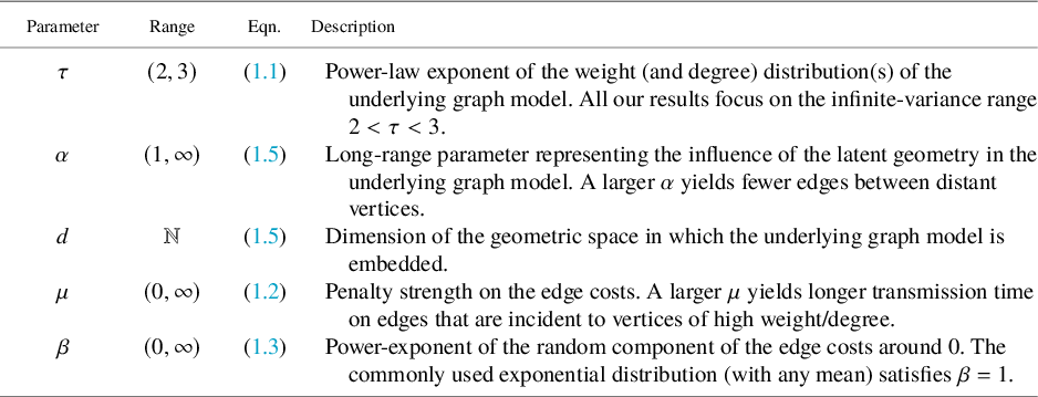
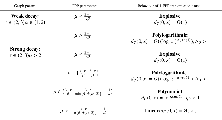


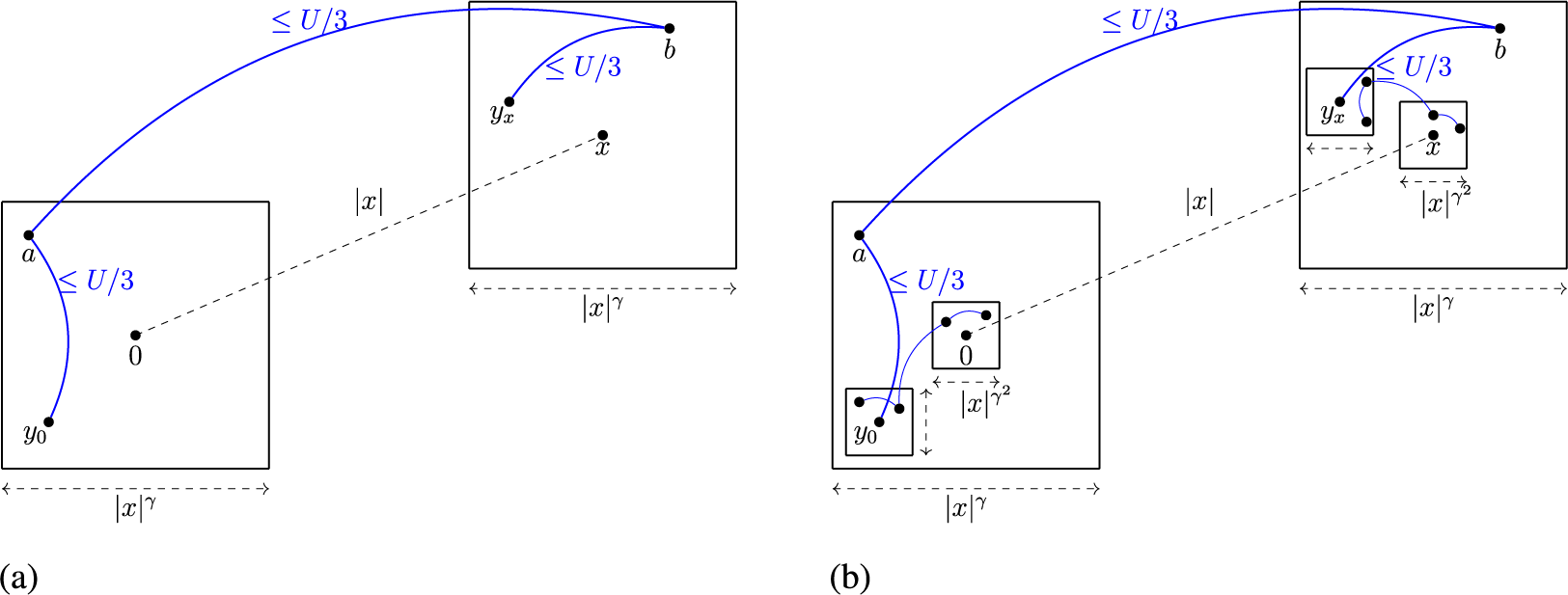
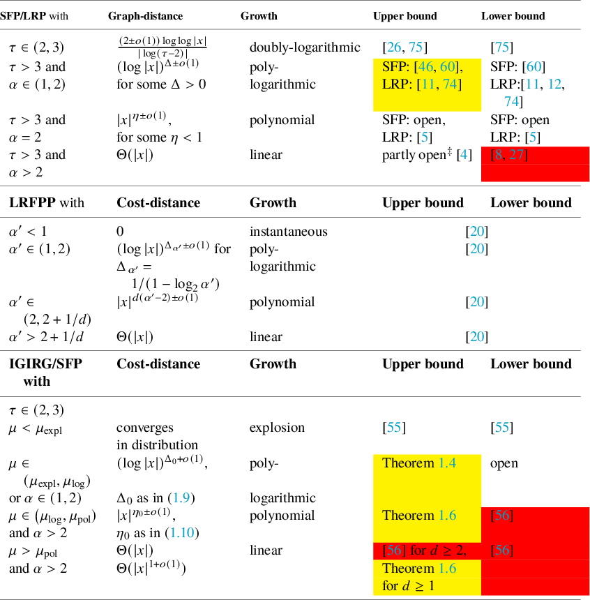

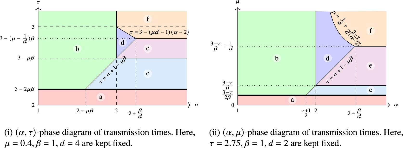


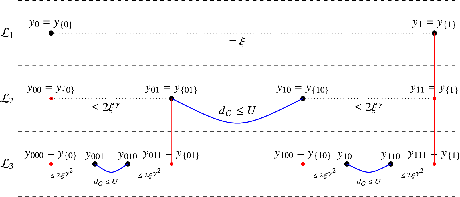


 Open access