Illustration

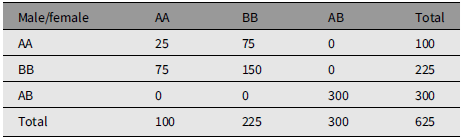
Table 1 gives the array of numbers of mating couples under random mating. The population has M ₁ = 100 males of type AA, M ₂ = 225 males of type BB, and M ₃ = 300 males of type AB. The population has an identical array of females with numbers F ₁, F ₂, and F ₃. The total number of males is N = 625, as is the number of females. C _ij is the number of couples in urn U_ij, that is, of type i in male and type j in female. C _ij = C _ji. N is the total number of couples. Gene A frequency is q = 0.4. Gene B frequency is p = .6. The marginal frequencies are Nq ², Np ², and 2Npq.

Table 1. An example of random mating

The marginal arrays are in HW form corresponding to gene frequencies q and 1 – q. The numbers in the body of Table 1 conform to ‘random mating’, being Nq ⁴, and so forth.

The offspring distribution is calculated from strictly Mendelian prescription with one child of each sex per couple. The number of male/female children of type AA is C ₁₁ + C ₁₃/2 + C ₃₁/2 + C ₃₃/4 = 100, that is, equal to the number of parents of each sex. The other genotypes are reproduced.

The main point to notice is that C ₃₃ = 4C ₁₂, so that C ₃₃ is a multiple of 4 for the illustration. A useful additional feature for the illustration is that C ₁₃ and C ₂₃ are even numbers.

The main point of this note is to illustrate that, starting from the same parental distribution, there is an infinite number of couplings that reproduce the parental distribution. This is done by the artifice of moving balls between urns. The urns are identified by the symbols U_ij, which hold the number of balls C _ij.

The process can be done in various ways, but a starting point is to vary C ₃₃ and move balls between urns in the same row or column keeping the marginal number constant. The number of degrees of freedom in the setup is one: varying one of the C _ij fixes the others automatically.

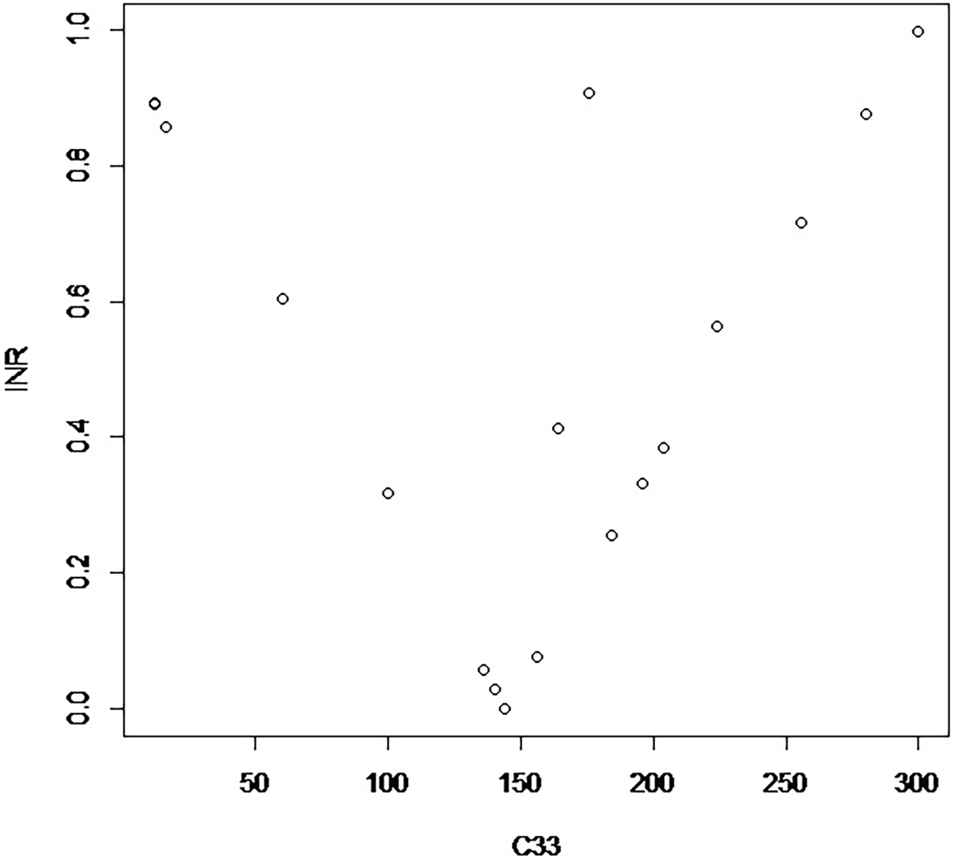
The proposed measure of divergence from random mating of a variant from the original table is Σ_ij|C_ij – H _ij|/N, where H refers to the table of randomly mating couples. Figure 1 displays the measure of divergence for an arbitrarily chosen group of couplings with the marginal array of parents with the same parental numbers as those in Table 1. There is a discernible pattern around the zero arising from random mating.

Figure 1. Display of calculated indices of divergence from random mating plotted against C ₃₃. These relate to the original population of males and females in Table 1.

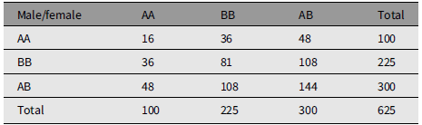
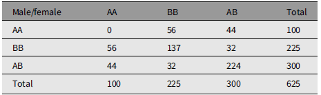
Table 2 is an example of mating whose measure of divergence is 0.5632. Table 3 is an extreme example of mating choice whose measure of divergence is 0.9984. There is no limit to the number of numerical examples starting from an array of parents in HW form.

Table 2. An example of nonrandom mating that reproduces Hardy-Weinberg frequencies. The measure of divergence from random mating is 0.5632

Table 3. An extreme example of nonrandom mating that reproduces Hardy-Weinberg frequencies. The measure of divergence from random mating is 0.9984

For most practical purposes attention would be focused on situations of divergence close to zero, so Figure 1 is only an indication of its properties and is based on an arbitrary set of cases starting from the numbers given in the margins of Table 1. The values of divergence given with Tables 2 and 3 fit on a straight line radiating to the right from the zero value of Table 1. More aberrant values can be constructed, as illustrated in Figure 1.

The illustration is contradictory, being a concrete example of an abstraction. Applications of the Hardy-Weinberg model to real problems are usually accompanied by caveats. While no one expects the abstraction to be followed precisely in practice it is of interest that matings of low divergence can reproduce the Hardy-Weinberg distribution. The user can select the gene frequency and the size of the population to achieve a desired level of precision and convenience.

Stochastic Processes

Johnson and Kotz (Reference Johnson and Kotz1977) have a section on applications of urn models in genetics. This was based on a draft supplied by W. J. Ewens. The approach is more sophisticated dealing with random fluctuations in the genetic composition of populations and sampling of populations. Johnson and Kotz (p. 239) give the basic formula for the change in a population from one generation to the next:

$${P_{ij}} = \left( {_j^m} \right){\left( {{i}\over{m}} \right)^j}{\left( {1 - {{i}\over{m}}} \right)^{m - j}}\,\,\,\,\,\,\,\,(\raise2pt{*})$$

Equation (*) gives the probability that a population of size m with i genes of the first allele changes in one generation to one having j copies of the allele. This is derived by drawing with replacement genes from one urn and putting them in a second urn. Johnson and Kotz use (*) to derive the probability that the population will eventually contain genes of the first type only as im ⁻¹.

Johnson and Kotz (Reference Johnson and Kotz1977) consider the way in which, as sampling of the kind described is repeated, only one of the original two alleles becomes fixed. They state that no simple explicit formula has been found for the mean number of urn replacements taken to achieve uniformity. Johnson and Kotz turn their attention to the diploid case, considering the probability that, in the sequence of draws from urns, two balls will be of the same allelic type. Their calculation shows that the loss of variation is slow, with the comment ‘this fact is of great importance in reconciling the Mendelian mechanism of inheritance with the Darwinian theory of natural selection, since it shows that genetic variation tends to be preserved for long time intervals and thus allows ample time for selective forces to act’ (p. 241). Johnson and Kotz appear to believe that there is plan and purpose in Nature.

Other more complex cases, including provision for mutation, are dealt with by Johnson and Kotz (Reference Johnson and Kotz1977). Since that time much has been written on reconstructing the past history of a population based on a sample of individuals taken at the present time. Since much of this is done without knowledge of the characteristics of the ancestry of the sample it is not easy to see how one could apply urn models to mimic the scenario.