











1 Introduction
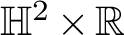
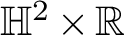
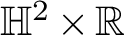
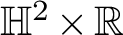
The theory of complete minimal surfaces in $\mathbb {H}^2\times \mathbb {R}$
with finite total curvature – that is, those whose Gauss curvature is integrable – has received considerable attention during the last decade, mainly triggered by Collin and Rosenberg [Reference Collin and Rosenberg2]. The combined work of Hauswirth, Nelli, Sa Earp, and Toubiana [Reference Hauswirth, Nelli, Earp and Toubiana6], and Hauswirth, Menezes, and Rodríguez [Reference Hauswirth, Menezes and Rodríguez5] shows that a complete minimal surface immersed in
$\mathbb {H}^2\times \mathbb {R}$
with finite total curvature – that is, those whose Gauss curvature is integrable – has received considerable attention during the last decade, mainly triggered by Collin and Rosenberg [Reference Collin and Rosenberg2]. The combined work of Hauswirth, Nelli, Sa Earp, and Toubiana [Reference Hauswirth, Nelli, Earp and Toubiana6], and Hauswirth, Menezes, and Rodríguez [Reference Hauswirth, Menezes and Rodríguez5] shows that a complete minimal surface immersed in $\mathbb {H}^2\times \mathbb {R}$
has finite total curvature if and only if it is proper, has finite topology, and has each of its ends asymptotic to an admissible polygon – that is, a curve homeomorphic to
$\mathbb {H}^2\times \mathbb {R}$
has finite total curvature if and only if it is proper, has finite topology, and has each of its ends asymptotic to an admissible polygon – that is, a curve homeomorphic to $\mathbb {S}^1$
consisting of finitely many alternating complete vertical and horizontal ideal geodesics (see [Reference Hauswirth, Menezes and Rodríguez5]). Here the product compactification of
$\mathbb {S}^1$
consisting of finitely many alternating complete vertical and horizontal ideal geodesics (see [Reference Hauswirth, Menezes and Rodríguez5]). Here the product compactification of $\mathbb {H}^2\times \mathbb {R}$
is considered, in which the horizontal (resp., vertical) ideal boundary consists of two disks
$\mathbb {H}^2\times \mathbb {R}$
is considered, in which the horizontal (resp., vertical) ideal boundary consists of two disks $\mathbb H^2\times \{\pm \infty \}$
(resp., the cylinder
$\mathbb H^2\times \{\pm \infty \}$
(resp., the cylinder $\partial _{\infty }\mathbb H^2\times \mathbb {R}$
). Ideal horizontal geodesics are those of the form
$\partial _{\infty }\mathbb H^2\times \mathbb {R}$
). Ideal horizontal geodesics are those of the form $\Gamma \times \{+\infty \}$
or
$\Gamma \times \{+\infty \}$
or $\Gamma \times \{-\infty \}$
, where
$\Gamma \times \{-\infty \}$
, where $\Gamma $
is a geodesic of
$\Gamma $
is a geodesic of $\mathbb H^2$
, whereas ideal vertical geodesics are those of the form
$\mathbb H^2$
, whereas ideal vertical geodesics are those of the form $\{p_{\infty }\}\times \mathbb {R}$
, where
$\{p_{\infty }\}\times \mathbb {R}$
, where $p_{\infty }\in \partial _{\infty }\mathbb H^2$
is an ideal point.
$p_{\infty }\in \partial _{\infty }\mathbb H^2$
is an ideal point.
Combining this classification with the previous work of Hauswirth and Rosenberg [Reference Hauswirth and Rosenberg7], the following Gauss–Bonnet-type formula for a complete minimal surface $\Sigma $
immersed in
$\Sigma $
immersed in $\mathbb {H}^2\times \mathbb {R}$
with finite total curvature holds true:
$\mathbb {H}^2\times \mathbb {R}$
with finite total curvature holds true:
 $$ \begin{align} \int_\Sigma K=2\pi\chi(\Sigma)-2\pi m=2\pi(2-2g-k-m), \end{align} $$
where g and k are, respectively, the genus and the number of ends of $\Sigma $
,
$\Sigma $
, $\chi (\Sigma )=2-2g-k$
its Euler characteristic, K its Gauss curvature, and m the total number of horizontal ideal geodesics in
$\chi (\Sigma )=2-2g-k$
its Euler characteristic, K its Gauss curvature, and m the total number of horizontal ideal geodesics in $\mathbb {H}^2\times \{+\infty \}$
, among all polygonal components associated with the ends of
$\mathbb {H}^2\times \{+\infty \}$
, among all polygonal components associated with the ends of $\Sigma $
. Observe that the union of all these components consists of m ideal horizontal geodesics in
$\Sigma $
. Observe that the union of all these components consists of m ideal horizontal geodesics in $\mathbb {H}^2\times \{+\infty \}$
, m ideal horizontal geodesics in
$\mathbb {H}^2\times \{+\infty \}$
, m ideal horizontal geodesics in $\mathbb {H}^2\times \{-\infty \}$
, and
$\mathbb {H}^2\times \{-\infty \}$
, and $2m$
ideal vertical geodesics, so the term
$2m$
ideal vertical geodesics, so the term $2\pi m$
in equation (1.1) can be understood as the sum of exterior angles of the asymptotic boundary of
$2\pi m$
in equation (1.1) can be understood as the sum of exterior angles of the asymptotic boundary of $\Sigma $
. We also remark that equation (1.1) has been extended to some quotients of
$\Sigma $
. We also remark that equation (1.1) has been extended to some quotients of $\mathbb {H}^2\times \mathbb {R}$
by Hauswirth and Menezes [Reference Hauswirth and Menezes4].
$\mathbb {H}^2\times \mathbb {R}$
by Hauswirth and Menezes [Reference Hauswirth and Menezes4].
Although this characterization is very satisfactory from a theoretical point of view, it seems tough in general to determine whether or not a given family of admissible polygons actually bounds a minimal surface, or if a given topological type can be realized by such a surface. In fact, there are not many examples of surfaces with finite total curvature in the literature. Let us highlight some of them in terms of the three parameters $(g,k,m)$
appearing in equation (1.1):
$(g,k,m)$
appearing in equation (1.1):
-
• The simplest case is that of flat minimal surfaces, which must be vertical planes (i.e., of the form $\Gamma \times \mathbb {R}$
, where
$\Gamma \subset \mathbb {H}^2$
is a complete geodesic) because of the Gauss equation. In particular, vertical planes are the only complete minimal surfaces with finite total curvature and
$(g,k,m)=(0,1,1)$
(see also [Reference Hauswirth, Sa Earp and Toubiana8, Corollary 5]).
$\Gamma \times \mathbb {R}$
, where
$\Gamma \subset \mathbb {H}^2$
is a complete geodesic) because of the Gauss equation. In particular, vertical planes are the only complete minimal surfaces with finite total curvature and
$(g,k,m)=(0,1,1)$
(see also [Reference Hauswirth, Sa Earp and Toubiana8, Corollary 5]). -
• A minimal Scherk graph in
$\mathbb {H}^2\times \mathbb {R}$
is a minimal graph over a geodesic ideal polygon of
$\mathbb {H}^2$
with
$2a$
vertices,
$a\geq 2$
, taking alternating limit values
$+\infty $
and
$-\infty $
on the sides of the polygon. A characterization of polygons carrying such a surface is analyzed in [Reference Mazet, Rodríguez and Rosenberg14], in which case they have finite total curvature and satisfy
$(g,k,m)=(0,1,a)$
. The case
$a=2$
gives rise to the only complete minimal surfaces with total curvature
$-2\pi $
, as shown by Pyo and Rodríguez [Reference Pyo and Rodríguez21, Theorem 4.1]. We can find as well the twisted Scherk minimal surfaces [Reference Pyo and Rodríguez21] with
$(g,k,m)=(0,1,2b+1)$
,
$b\geq 1$
, and total curvature
$-4b\pi $
that are no longer graphs or bigraphs, some of which are embedded. -
• Minimal k-noids constructed by Morabito and Rodríguez [Reference Morabito and Rodríguez16] (also by Pyo [Reference Pyo20] in the symmetric case) have finite total curvature, genus
$0$
, and k ends asymptotic to vertical planes. This gives
$g=0$
and
$k=m\geq 2$
. -
• Horizontal catenoids are the only complete minimal surfaces immersed in
$\mathbb {H}^2\times \mathbb {R}$
with finite total curvature and
$k=m=2$
(see [Reference Hauswirth, Menezes and Rodríguez5, Reference Hauswirth, Nelli, Earp and Toubiana6]). The family of minimal surfaces with finite total curvature and
$k=m\geq 3$
is not hitherto well understood, not even in the case
$g=0$
. The most general construction was given by Martín, Mazzeo, and Rodríguez [Reference Martín, Mazzeo and Rodríguez12], who found properly embedded minimal surfaces with finite total curvature in
$\mathbb {H}^2\times \mathbb {R}$
of genus g and k ends asymptotic to vertical planes (and hence
$m=k$
), for arbitrary
$g\geq 0$
and k arbitrarily large depending on g.


In this paper we provide highly symmetric examples with $g=1$
and
$g=1$
and $m=k\geq 3$
, which are hence conformally equivalent to a torus with k punctures. They can be thought of as the counterpart in
$m=k\geq 3$
, which are hence conformally equivalent to a torus with k punctures. They can be thought of as the counterpart in $\mathbb {H}^2\times \mathbb {R}$
of the genus
$\mathbb {H}^2\times \mathbb {R}$
of the genus $1$
minimal k-noids in
$1$
minimal k-noids in $\mathbb {R}^3$
obtained by Mazet [Reference Mazet13]. Outside a compact subset, our surfaces look like the minimal k-noids in [Reference Morabito and Rodríguez16, Reference Pyo20], and they are not globally embedded in general. Notice that there are no such examples with
$\mathbb {R}^3$
obtained by Mazet [Reference Mazet13]. Outside a compact subset, our surfaces look like the minimal k-noids in [Reference Morabito and Rodríguez16, Reference Pyo20], and they are not globally embedded in general. Notice that there are no such examples with $k=2$
, due to the aforesaid uniqueness of horizontal catenoids in [Reference Hauswirth, Nelli, Earp and Toubiana6]. Our main result can be stated as follows:
$k=2$
, due to the aforesaid uniqueness of horizontal catenoids in [Reference Hauswirth, Nelli, Earp and Toubiana6]. Our main result can be stated as follows:
Theorem 1. For each $k\geq 3$
, there exists a
$k\geq 3$
, there exists a $1$
-parameter family of properly Alexandrov-embedded minimal surfaces in
$1$
-parameter family of properly Alexandrov-embedded minimal surfaces in $\mathbb {H}^2\times \mathbb {R}$
with genus
$\mathbb {H}^2\times \mathbb {R}$
with genus $1$
and k ends, dihedrally symmetric with respect to k vertical planes and symmetric with respect to a horizontal plane. They have finite total curvature
$1$
and k ends, dihedrally symmetric with respect to k vertical planes and symmetric with respect to a horizontal plane. They have finite total curvature $-4k\pi $
, and each of their ends is embedded and asymptotic to a vertical plane.
$-4k\pi $
, and each of their ends is embedded and asymptotic to a vertical plane.
The construction of these genus $1$
minimal k-noids is based on a conjugate technique, in the sense of Daniel [Reference Daniel3] and Hauswirth, Sa Earp, and Toubiana [Reference Hauswirth, Sa Earp and Toubiana8]. Conjugation has been a fruitful technique to obtain constant-mean-curvature surfaces in
$1$
minimal k-noids is based on a conjugate technique, in the sense of Daniel [Reference Daniel3] and Hauswirth, Sa Earp, and Toubiana [Reference Hauswirth, Sa Earp and Toubiana8]. Conjugation has been a fruitful technique to obtain constant-mean-curvature surfaces in $\mathbb {H}^2\times \mathbb {R}$
and
$\mathbb {H}^2\times \mathbb {R}$
and $\mathbb {S}^2\times \mathbb {R}$
(see [Reference Manzano and Torralbo10, Reference Manzano, Plehnert and Torralbo11, Reference Manzano and Torralbo9, Reference Mazet13, Reference Mazet, Rodríguez and Rosenberg15, Reference Morabito and Rodríguez16, Reference Plehnert19, Reference Plehnert18, Reference Pyo20] and the references therein). We begin by considering a solution to an improper Dirichlet problem [Reference Mazet, Rodríguez and Rosenberg14, Reference Nelli and Rosenberg17] in
$\mathbb {S}^2\times \mathbb {R}$
(see [Reference Manzano and Torralbo10, Reference Manzano, Plehnert and Torralbo11, Reference Manzano and Torralbo9, Reference Mazet13, Reference Mazet, Rodríguez and Rosenberg15, Reference Morabito and Rodríguez16, Reference Plehnert19, Reference Plehnert18, Reference Pyo20] and the references therein). We begin by considering a solution to an improper Dirichlet problem [Reference Mazet, Rodríguez and Rosenberg14, Reference Nelli and Rosenberg17] in $\mathbb {H}^2\times \mathbb {R}$
over an unbounded geodesic triangle
$\mathbb {H}^2\times \mathbb {R}$
over an unbounded geodesic triangle $\Delta \subset \mathbb {H}^2$
, a so-called Jenkins–Serrin problem [Reference Mazet, Rodríguez and Rosenberg14]. These solutions are minimal graphs over the interior of
$\Delta \subset \mathbb {H}^2$
, a so-called Jenkins–Serrin problem [Reference Mazet, Rodríguez and Rosenberg14]. These solutions are minimal graphs over the interior of $\Delta $
with prescribed finite and infinite values when one approaches
$\Delta $
with prescribed finite and infinite values when one approaches $\partial \Delta $
. The conjugate surface is another minimal graph in
$\partial \Delta $
. The conjugate surface is another minimal graph in $\mathbb {H}^2\times \mathbb {R}$
whose boundary is made of curves lying on totally geodesic surfaces – that is, vertical and horizontal planes. Since there are isometric reflections across such planes in
$\mathbb {H}^2\times \mathbb {R}$
whose boundary is made of curves lying on totally geodesic surfaces – that is, vertical and horizontal planes. Since there are isometric reflections across such planes in $\mathbb {H}^2\times \mathbb {R}$
, the conjugate surface can be extended to a complete surface under suitable conditions. In order to prescribe the symmetries stated in Theorem 1, we will encounter two period problems that will impose further restrictions on
$\mathbb {H}^2\times \mathbb {R}$
, the conjugate surface can be extended to a complete surface under suitable conditions. In order to prescribe the symmetries stated in Theorem 1, we will encounter two period problems that will impose further restrictions on $\Delta $
and on the boundary values of the Jenkins–Serrin problem.
$\Delta $
and on the boundary values of the Jenkins–Serrin problem.
Our conjugate approach is inspired by the genus $1$
minimal k-noids in
$1$
minimal k-noids in $\mathbb {R}^3$
given by Mazet [Reference Mazet13], and by the mean-curvature
$\mathbb {R}^3$
given by Mazet [Reference Mazet13], and by the mean-curvature $\frac {1}{2}$
surfaces in
$\frac {1}{2}$
surfaces in $\mathbb {H}^2\times \mathbb {R}$
given by Plehnert [Reference Plehnert19]. It is important to remark that there exist technical dissimilarities between the cases
$\mathbb {H}^2\times \mathbb {R}$
given by Plehnert [Reference Plehnert19]. It is important to remark that there exist technical dissimilarities between the cases $H=0$
and
$H=0$
and $H=\frac {1}{2}$
in
$H=\frac {1}{2}$
in $\mathbb {H}^2\times \mathbb {R}$
, because of the fact that the conjugate of a surface with mean curvature
$\mathbb {H}^2\times \mathbb {R}$
, because of the fact that the conjugate of a surface with mean curvature $\frac {1}{2}$
(resp.,
$\frac {1}{2}$
(resp., $0$
) is a minimal surface in the Heisenberg group
$0$
) is a minimal surface in the Heisenberg group $\mathrm {Nil}_3$
(resp.,
$\mathrm {Nil}_3$
(resp., $\mathbb {H}^2\times \mathbb {R}$
). Furthermore, our construction can be adapted to produce complete minimal surfaces that are invariant by an arbitrary vertical translation (i.e., in the direction of the factor
$\mathbb {H}^2\times \mathbb {R}$
). Furthermore, our construction can be adapted to produce complete minimal surfaces that are invariant by an arbitrary vertical translation (i.e., in the direction of the factor $\mathbb {R}$
), similar to the saddle towers given in [Reference Morabito and Rodríguez16]. They have genus
$\mathbb {R}$
), similar to the saddle towers given in [Reference Morabito and Rodríguez16]. They have genus $1$
in the quotient and they are not embedded in general.
$1$
in the quotient and they are not embedded in general.
Theorem 2. For each $k\geq 3$
and each vertical translation T, there is a
$k\geq 3$
and each vertical translation T, there is a $1$
-parameter family of Alexandrov-embedded singly periodic minimal surfaces in
$1$
-parameter family of Alexandrov-embedded singly periodic minimal surfaces in $\mathbb {H}^2\times \mathbb {R}$
that are invariant by T and dihedrally symmetric with respect to k vertical planes and a horizontal plane. They have finite total curvature
$\mathbb {H}^2\times \mathbb {R}$
that are invariant by T and dihedrally symmetric with respect to k vertical planes and a horizontal plane. They have finite total curvature $-4k\pi $
, genus
$-4k\pi $
, genus $1$
, and
$1$
, and $2k$
vertical ends in the quotient of
$2k$
vertical ends in the quotient of $\mathbb {H}^2\times \mathbb {R}$
by T.
$\mathbb {H}^2\times \mathbb {R}$
by T.
Our analysis of the period problems will allow us to find surfaces that are invariant not by a discrete group of rotations but by discrete groups of parabolic or hyperbolic translations, which we will call parabolic and hyperbolic $\infty $
-noids, respectively. These surfaces have infinitely many ends, and we can guarantee that many of the examples are properly embedded in the hyperbolic case. Although we will not state it explicitly, analogous surfaces can be obtained in the quotient of
$\infty $
-noids, respectively. These surfaces have infinitely many ends, and we can guarantee that many of the examples are properly embedded in the hyperbolic case. Although we will not state it explicitly, analogous surfaces can be obtained in the quotient of $\mathbb {H}^2\times \mathbb {R}$
by an arbitrary vertical translation in the spirit of Theorem 2, giving rise to doubly periodic examples in which the Hauswirth–Menezes formula [Reference Hauswirth and Menezes4] for finite-total-curvature surfaces applies in the quotient.
$\mathbb {H}^2\times \mathbb {R}$
by an arbitrary vertical translation in the spirit of Theorem 2, giving rise to doubly periodic examples in which the Hauswirth–Menezes formula [Reference Hauswirth and Menezes4] for finite-total-curvature surfaces applies in the quotient.
Theorem 3. There is a $2$
-parameter (resp.,
$2$
-parameter (resp., $1$
-parameter) family of properly embedded (resp., Alexandrov-embedded) minimal surfaces in
$1$
-parameter) family of properly embedded (resp., Alexandrov-embedded) minimal surfaces in $\mathbb {H}^2\times \mathbb {R}$
with genus
$\mathbb {H}^2\times \mathbb {R}$
with genus $0$
and infinitely many ends, invariant by a discrete group of hyperbolic (resp., parabolic) translations. Each of their ends is embedded and asymptotic to a vertical plane, and has finite total curvature.
$0$
and infinitely many ends, invariant by a discrete group of hyperbolic (resp., parabolic) translations. Each of their ends is embedded and asymptotic to a vertical plane, and has finite total curvature.
The paper is organized as follows: In §2 we will analyze some aspects of the conjugation of surfaces in $\mathbb {H}^2\times \mathbb {R}$
that will be needed in the construction, and §3 will be devoted to filling in the details of the proofs of Theorems 1 and 2. We will also discuss some open questions about the uniqueness and embeddedness of the constructed surfaces, as well as natural limits of the
$\mathbb {H}^2\times \mathbb {R}$
that will be needed in the construction, and §3 will be devoted to filling in the details of the proofs of Theorems 1 and 2. We will also discuss some open questions about the uniqueness and embeddedness of the constructed surfaces, as well as natural limits of the $1$
-parameter family of genus
$1$
-parameter family of genus $1\ k$
-noids. In the last part of the paper we will prove Theorem 3.
$1\ k$
-noids. In the last part of the paper we will prove Theorem 3.
2 Preliminaries
Let $\Sigma $
be a simply connected Riemannian surface. Given an isometric minimal immersion
$\Sigma $
be a simply connected Riemannian surface. Given an isometric minimal immersion $X:\Sigma \to \mathbb {H}^2\times \mathbb {R}$
, Hauswirth, Sa Earp, and Toubiana [Reference Hauswirth, Sa Earp and Toubiana8] proved the existence of another isometric minimal immersion
$X:\Sigma \to \mathbb {H}^2\times \mathbb {R}$
, Hauswirth, Sa Earp, and Toubiana [Reference Hauswirth, Sa Earp and Toubiana8] proved the existence of another isometric minimal immersion $\widetilde X:\Sigma \to \mathbb {H}^2\times \mathbb {R}$
such that the following are true:
$\widetilde X:\Sigma \to \mathbb {H}^2\times \mathbb {R}$
such that the following are true:
-
(1) Both immersions induce the same angle function
$\nu =\langle N,\partial _t\rangle =\langle \widetilde N,\partial _t\rangle $
, where N and
$\widetilde N$
stand for unit normal vector fields to X and
$\widetilde X$
, respectively, and
$\partial _t$
is the unit vector field in
$\mathbb {H}^2\times \mathbb {R}$
in the direction of the factor
$\mathbb {R}$
. -
(2) The shape operators S and
$\widetilde S$
of X and
$\widetilde X$
, respectively, satisfy
$\widetilde S=JS$
, where J is the
$\frac \pi 2$
-rotation in
$T\Sigma $
, chosen such that both
$\left \{\mathrm {d}X_p(u),\mathrm {d}X_p(Ju),N_p\right \}$
and
$\{\mathrm {d}\widetilde X_p(u),\mathrm {d}\widetilde X_p(Ju),\widetilde N_p \}$
are positively oriented bases in
$\mathbb H^2\times \mathbb R$
for all nonzero tangent vectors
$u\in T_p\Sigma $
. -
(3) The tangential components
$T=\partial _t-\nu N$
and
$\widetilde T=\partial _t-\nu \widetilde N$
of
$\partial _t$
satisfy
$\widetilde X^*\widetilde T=JX^*T$
. This implies that
$\langle \mathrm {d}X_p(u),\partial _t\rangle =\langle \mathrm {d}\widetilde X_p(Ju),\partial _t\rangle $
for all
$u\in T_p\Sigma $
.


The immersions X and $\widetilde X$
are called conjugate and determine each other up to ambient isometries preserving both the global orientation and the vector field
$\widetilde X$
are called conjugate and determine each other up to ambient isometries preserving both the global orientation and the vector field $\partial _t$
. Our initial surface
$\partial _t$
. Our initial surface $X(\Sigma )$
will be a vertical graph over a convex domain, namely a solution of a Jenkins–Serrin problem. This implies that
$X(\Sigma )$
will be a vertical graph over a convex domain, namely a solution of a Jenkins–Serrin problem. This implies that $\widetilde X(\Sigma )$
is also a vertical graph over another (possibly nonconvex) domain, due to the Krust-type theorem given by [Reference Hauswirth, Sa Earp and Toubiana8, Theorem 14]. Therefore, we can assume that both surfaces are embedded, and we will use the notation
$\widetilde X(\Sigma )$
is also a vertical graph over another (possibly nonconvex) domain, due to the Krust-type theorem given by [Reference Hauswirth, Sa Earp and Toubiana8, Theorem 14]. Therefore, we can assume that both surfaces are embedded, and we will use the notation $\Sigma $
and
$\Sigma $
and $\widetilde \Sigma $
for the surfaces
$\widetilde \Sigma $
for the surfaces $X(\Sigma )$
and
$X(\Sigma )$
and $\widetilde X(\Sigma )$
, respectively.
$\widetilde X(\Sigma )$
, respectively.
Although the conjugate surface $\widetilde \Sigma $
is not explicit in general, one can obtain insightful information if the initial surface
$\widetilde \Sigma $
is not explicit in general, one can obtain insightful information if the initial surface $\Sigma $
has boundary consisting of horizontal and vertical geodesics intersecting at some vertices. A curve
$\Sigma $
has boundary consisting of horizontal and vertical geodesics intersecting at some vertices. A curve $\Gamma \subset \Sigma $
is a horizontal (resp., vertical) geodesic in
$\Gamma \subset \Sigma $
is a horizontal (resp., vertical) geodesic in $\mathbb {H}^2\times \mathbb {R}$
if and only if the conjugate curve
$\mathbb {H}^2\times \mathbb {R}$
if and only if the conjugate curve $\widetilde \Gamma \subset \widetilde \Sigma $
lies in a vertical (resp., horizontal) totally geodesic surface of
$\widetilde \Gamma \subset \widetilde \Sigma $
lies in a vertical (resp., horizontal) totally geodesic surface of $\mathbb {H}^2\times \mathbb {R}$
intersecting
$\mathbb {H}^2\times \mathbb {R}$
intersecting $\widetilde \Sigma $
orthogonally along
$\widetilde \Sigma $
orthogonally along $\widetilde \Gamma $
. Furthermore, axial symmetry about
$\widetilde \Gamma $
. Furthermore, axial symmetry about $\Gamma $
corresponds to mirror symmetry about
$\Gamma $
corresponds to mirror symmetry about $\widetilde \Gamma $
, which enables analytic continuation of
$\widetilde \Gamma $
, which enables analytic continuation of $\Sigma $
and
$\Sigma $
and $\widetilde \Sigma $
across their boundaries. If the angles at the vertices of
$\widetilde \Sigma $
across their boundaries. If the angles at the vertices of $\partial \Sigma $
are integer divisors of
$\partial \Sigma $
are integer divisors of $\pi $
, then no singularity appears at such vertices after successive reflections about the boundary components, and both surfaces can be extended to complete (possibly nonembedded) minimal surfaces. We refer to [Reference Manzano and Torralbo10, Reference Plehnert19, Reference Mazet, Rodríguez and Rosenberg15] for details.
$\pi $
, then no singularity appears at such vertices after successive reflections about the boundary components, and both surfaces can be extended to complete (possibly nonembedded) minimal surfaces. We refer to [Reference Manzano and Torralbo10, Reference Plehnert19, Reference Mazet, Rodríguez and Rosenberg15] for details.
However, most difficulties concerning the depiction of $\widetilde \Sigma $
, and in particular deciding whether or not it is embedded, show up when one tries to understand the behavior of the conjugate of a vertical geodesic. We will now recall some properties on this matter, which will be used later in §3. Let
$\widetilde \Sigma $
, and in particular deciding whether or not it is embedded, show up when one tries to understand the behavior of the conjugate of a vertical geodesic. We will now recall some properties on this matter, which will be used later in §3. Let $\gamma :I\to \partial \Sigma $
be a vertical geodesic with unit speed such that
$\gamma :I\to \partial \Sigma $
be a vertical geodesic with unit speed such that $\gamma '=\partial _t$
(this orientation of vertical geodesics will be fixed throughout the text), where
$\gamma '=\partial _t$
(this orientation of vertical geodesics will be fixed throughout the text), where $I\subset \mathbb {R}$
is an interval, and denote by
$I\subset \mathbb {R}$
is an interval, and denote by $\widetilde \gamma :I\to \partial \widetilde \Sigma $
the conjugate curve, which will be assumed to lie in
$\widetilde \gamma :I\to \partial \widetilde \Sigma $
the conjugate curve, which will be assumed to lie in $\mathbb {H}^2\times \{0\}$
after a vertical translation.
$\mathbb {H}^2\times \{0\}$
after a vertical translation.
Let us consider the half-space model $\mathbb {H}^2\times \mathbb {R}=\left \{(x,y,t)\in \mathbb {R}^3:y>0\right \}$
, whose metric is given by
$\mathbb {H}^2\times \mathbb {R}=\left \{(x,y,t)\in \mathbb {R}^3:y>0\right \}$
, whose metric is given by $y^{-2}\left (\mathrm {d}x^2+\mathrm {d}y^2\right )+\mathrm {d}t^2$
, with positively oriented orthonormal frame
$y^{-2}\left (\mathrm {d}x^2+\mathrm {d}y^2\right )+\mathrm {d}t^2$
, with positively oriented orthonormal frame $\{E_1,E_2,\partial _t\}$
given by
$\{E_1,E_2,\partial _t\}$
given by $E_1=y\partial _x$
and
$E_1=y\partial _x$
and $E_2=y\partial _y$
(observe that
$E_2=y\partial _y$
(observe that $E_1$
is tangent to the foliation of
$E_1$
is tangent to the foliation of $\mathbb {H}^2$
by horocycles
$\mathbb {H}^2$
by horocycles $y=y_0$
, with
$y=y_0$
, with $y_0>0$
). Since
$y_0>0$
). Since $\gamma $
is vertical and
$\gamma $
is vertical and $\widetilde \gamma $
lies in a horizontal slice, there exist smooth functions
$\widetilde \gamma $
lies in a horizontal slice, there exist smooth functions $\psi ,\theta \in C^\infty (I)$
such that
$\psi ,\theta \in C^\infty (I)$
such that
 $$ \begin{align} N_{\gamma(t)}&=\cos(\psi(t))E_1+\sin(\psi(t))E_2, \end{align} $$
 $$ \begin{align} \widetilde\gamma'(t)&=\cos(\theta(t))E_1+\sin(\theta(t))E_2, \end{align} $$
called, respectively, the angle of rotation of N along $\gamma $
and the angle of rotation of
$\gamma $
and the angle of rotation of $\widetilde \gamma $
with respect to the foliation by horocycles. We now collect some relations between these quantities (see also [Reference Castro-Infantes, Manzano and Rodríguez1, Reference Manzano and Torralbo9, Reference Plehnert19]).
$\widetilde \gamma $
with respect to the foliation by horocycles. We now collect some relations between these quantities (see also [Reference Castro-Infantes, Manzano and Rodríguez1, Reference Manzano and Torralbo9, Reference Plehnert19]).
Observe that $E_1$
and
$E_1$
and $E_2$
are parallel vector fields along
$E_2$
are parallel vector fields along $\gamma $
, since they satisfy
$\gamma $
, since they satisfy $\overline \nabla _{\partial _t}E_1=\overline \nabla _{\partial _t}E_2=0$
, where
$\overline \nabla _{\partial _t}E_1=\overline \nabla _{\partial _t}E_2=0$
, where $\overline \nabla $
stands for the ambient Levi-Civita connection. This is due to the facts that that
$\overline \nabla $
stands for the ambient Levi-Civita connection. This is due to the facts that that $\mathbb H^2\times \mathbb {R}$
is a Riemannian product and
$\mathbb H^2\times \mathbb {R}$
is a Riemannian product and $E_1$
and
$E_1$
and $E_2$
do not depend on the variable t. By taking derivatives in equation (2.1), we get
$E_2$
do not depend on the variable t. By taking derivatives in equation (2.1), we get $\overline \nabla _{\gamma '}N=-\psi '\sin (\psi )E_1+\psi '\cos (\psi )E_2=-\psi ' N\times \gamma '$
, where
$\overline \nabla _{\gamma '}N=-\psi '\sin (\psi )E_1+\psi '\cos (\psi )E_2=-\psi ' N\times \gamma '$
, where $\times $
is the cross-product in
$\times $
is the cross-product in $\mathbb H^2\times \mathbb {R}$
. Using the properties of the conjugation, we deduce the identity
$\mathbb H^2\times \mathbb {R}$
. Using the properties of the conjugation, we deduce the identity
 $$ \begin{align} \psi'=-\left\langle\overline\nabla_{\gamma'}N,N\times\gamma'\right\rangle=\langle S\gamma',J\gamma'\rangle=-\left\langle J\widetilde S\widetilde\gamma',J\widetilde\gamma'\right\rangle=\left\langle\overline\nabla_{\widetilde\gamma'}\widetilde N,\widetilde\gamma'\right\rangle=-\kappa_g, \end{align} $$
where $\kappa _g$
is the geodesic curvature of
$\kappa _g$
is the geodesic curvature of $\widetilde \gamma $
as a curve of
$\widetilde \gamma $
as a curve of $\mathbb {H}^2\times \{0\}$
with respect to the conormal
$\mathbb {H}^2\times \{0\}$
with respect to the conormal $\widetilde N$
(recall that
$\widetilde N$
(recall that $\widetilde \Sigma $
intersects
$\widetilde \Sigma $
intersects $\mathbb {H}^2\times \{0\}$
orthogonally). Now we will obtain further information under the additional assumption that the surfaces are multigraphs – that is, their common angle function
$\mathbb {H}^2\times \{0\}$
orthogonally). Now we will obtain further information under the additional assumption that the surfaces are multigraphs – that is, their common angle function $\nu $
has a sign.
$\nu $
has a sign.
Lemma 1. Assume that the interiors of $\Sigma $
and
$\Sigma $
and $\widetilde \Sigma $
are multigraphs over (possibly nonembedded) domains
$\widetilde \Sigma $
are multigraphs over (possibly nonembedded) domains $\Omega $
and
$\Omega $
and $\widetilde \Omega $
, respectively, with angle function
$\widetilde \Omega $
, respectively, with angle function $\nu>0$
, and let
$\nu>0$
, and let $\gamma $
be a vertical geodesic in
$\gamma $
be a vertical geodesic in $\partial \Sigma $
with
$\partial \Sigma $
with $\gamma '=\partial _t$
. In the notation already given:
$\gamma '=\partial _t$
. In the notation already given:
-
(a) If
$\psi '>0$
, then
$J\gamma ' \ (\text {resp., }J\widetilde \gamma '=\partial _t )$
is a unit outer conormal to
$\Sigma (\text {resp., }\widetilde \Sigma )$
along
$\gamma $
(resp.
$\widetilde \gamma $
),
$\widetilde N$
points to the interior of
$\widetilde \Omega $
along
$\widetilde \gamma $
, and
$\widetilde \Sigma $
lies in
$\mathbb {H}^2\times (-\infty ,0]$
locally around
$\widetilde \gamma $
(see Figure 1, top).Figure 1Orientation of the conjugate surfaces
$\Sigma $
and
$\widetilde \Sigma $
according to the direction of rotation of N along a vertical geodesic
$\gamma $
. -
(b) If
$\psi '<0$
, then
$J\gamma ' \ (\text {resp., }J\widetilde \gamma '=\partial _t )$
is a unit inner conormal to
$\Sigma (\text {resp. }\widetilde \Sigma)$
along
$\gamma $
(resp.
$\widetilde \gamma $
),
$\widetilde N$
points to the exterior of
$\widetilde \Omega $
along
$\widetilde \gamma $
, and
$\widetilde \Sigma $
lies in
$\mathbb {H}^2\times [0,+\infty )$
locally around
$\widetilde \gamma $
(see Figure 1, bottom).


Either way, the identity $\theta '=\psi '-\cos (\theta )$
holds true.
$\theta '=\psi '-\cos (\theta )$
holds true.
Proof. We will prove only (a), since (b) is analogous, so we will suppose that $\psi '>0$
. Observe that the normal N points upward in the interior of
$\psi '>0$
. Observe that the normal N points upward in the interior of $\Sigma $
, which is locally a graph by the assumption
$\Sigma $
, which is locally a graph by the assumption $\nu>0$
. This argument is not valid along
$\nu>0$
. This argument is not valid along $\gamma $
, where
$\gamma $
, where $\nu =0$
, but we infer by continuity that N is a horizontal
$\nu =0$
, but we infer by continuity that N is a horizontal $\frac {\pi }{2}$
-rotation of the outer unit conormal to
$\frac {\pi }{2}$
-rotation of the outer unit conormal to $\Sigma $
along
$\Sigma $
along $\gamma $
(this rotation is counterclockwise in a horizontal slice, in view of the condition
$\gamma $
(this rotation is counterclockwise in a horizontal slice, in view of the condition $\psi '>0$
). Hence,
$\psi '>0$
). Hence, $J\gamma '=N\times \gamma '$
is determined by the ambient orientation and points outside
$J\gamma '=N\times \gamma '$
is determined by the ambient orientation and points outside $\Sigma $
along
$\Sigma $
along $\gamma $
, as depicted in Figure 1 (top left). Since the rotation J is intrinsic, we deduce that
$\gamma $
, as depicted in Figure 1 (top left). Since the rotation J is intrinsic, we deduce that $J\widetilde \gamma '$
points outside
$J\widetilde \gamma '$
points outside $\widetilde \Sigma $
along
$\widetilde \Sigma $
along $\widetilde \gamma $
, and
$\widetilde \gamma $
, and $\widetilde N=\widetilde \gamma '\times J\widetilde \gamma '$
is also determined, as shown in Figure 1 (top right).
$\widetilde N=\widetilde \gamma '\times J\widetilde \gamma '$
is also determined, as shown in Figure 1 (top right).
Assume now by contradiction that $\widetilde N$
points to the exterior of
$\widetilde N$
points to the exterior of $\widetilde \Omega $
at some point p of
$\widetilde \Omega $
at some point p of $\widetilde \gamma $
. Since
$\widetilde \gamma $
. Since $\kappa _g=-\psi '<0$
with respect to the conormal
$\kappa _g=-\psi '<0$
with respect to the conormal $\widetilde N$
and
$\widetilde N$
and $\nu>0$
, we infer that
$\nu>0$
, we infer that $\widetilde \Sigma $
projects locally into the convex side of
$\widetilde \Sigma $
projects locally into the convex side of $\widetilde \gamma $
. This yields a contradiction with the boundary maximum principle by comparing
$\widetilde \gamma $
. This yields a contradiction with the boundary maximum principle by comparing $\widetilde \Sigma $
and a vertical plane tangent to
$\widetilde \Sigma $
and a vertical plane tangent to $\widetilde \gamma $
at p. Note that
$\widetilde \gamma $
at p. Note that $J\widetilde \gamma '$
cannot be equal to
$J\widetilde \gamma '$
cannot be equal to $-\partial _t$
(so it must be
$-\partial _t$
(so it must be $J\widetilde \gamma '=\partial _t)$
because it points outside
$J\widetilde \gamma '=\partial _t)$
because it points outside $\widetilde \Sigma $
along
$\widetilde \Sigma $
along $\widetilde \gamma $
and the angle function is positive. As a consequence, a neighborhood of
$\widetilde \gamma $
and the angle function is positive. As a consequence, a neighborhood of $\widetilde \gamma $
in
$\widetilde \gamma $
in $\widetilde \Sigma $
is contained in
$\widetilde \Sigma $
is contained in $\mathbb {H}^2\times (-\infty ,0]$
.
$\mathbb {H}^2\times (-\infty ,0]$
.
It is easy to calculate $\overline \nabla _{E_1}E_1=E_2$
,
$\overline \nabla _{E_1}E_1=E_2$
, $\overline \nabla _{E_1}E_2=-E_1$
, and
$\overline \nabla _{E_1}E_2=-E_1$
, and $\overline \nabla _{E_2}E_1=\overline \nabla _{E_2}E_2=0$
by using the expressions of
$\overline \nabla _{E_2}E_1=\overline \nabla _{E_2}E_2=0$
by using the expressions of $E_1$
and
$E_1$
and $E_2$
and the Koszul formula. On the one hand, this allows us to take derivatives in equation (2.2) to obtain
$E_2$
and the Koszul formula. On the one hand, this allows us to take derivatives in equation (2.2) to obtain $\overline \nabla _{\widetilde \gamma '}\widetilde \gamma '=(\theta '+\cos (\theta ))(-\sin (\theta )E_1+\cos (\theta )E_2)$
. On the other hand, the foregoing discussion shows that
$\overline \nabla _{\widetilde \gamma '}\widetilde \gamma '=(\theta '+\cos (\theta ))(-\sin (\theta )E_1+\cos (\theta )E_2)$
. On the other hand, the foregoing discussion shows that $\widetilde N=\widetilde \gamma '\times J\widetilde \gamma '=\widetilde \gamma '\times \partial _t=\sin (\theta )E_1-\cos (\theta )E_2$
, so the last identity in the statement follows from plugging these computations in the expression
$\widetilde N=\widetilde \gamma '\times J\widetilde \gamma '=\widetilde \gamma '\times \partial _t=\sin (\theta )E_1-\cos (\theta )E_2$
, so the last identity in the statement follows from plugging these computations in the expression $-\psi '=\kappa _g=\langle \overline \nabla _{\widetilde \gamma '}\widetilde \gamma ',\widetilde N \rangle $
.
$-\psi '=\kappa _g=\langle \overline \nabla _{\widetilde \gamma '}\widetilde \gamma ',\widetilde N \rangle $
.
3 Construction of genus
$1$
saddle towers and k-noids

The first part of this section is devoted to proving Theorems 1 and 2. The arguments leading to these results are based on a conjugate construction that depends on a parameter $0<l\leq \infty $
that will be fixed henceforth. The case
$0<l\leq \infty $
that will be fixed henceforth. The case $0<l<\infty $
gives the saddle towers whose fundamental pieces lie in a slab of height l, whereas the case
$0<l<\infty $
gives the saddle towers whose fundamental pieces lie in a slab of height l, whereas the case $l=\infty $
gives rise to the k-noids. Although a limit argument for
$l=\infty $
gives rise to the k-noids. Although a limit argument for $l\to \infty $
would imply the latter (as in [Reference Morabito and Rodríguez16]), we will discuss both cases together.
$l\to \infty $
would imply the latter (as in [Reference Morabito and Rodríguez16]), we will discuss both cases together.
3.1 The conjugate construction
Let $\Delta $
be a geodesic triangle with sides
$\Delta $
be a geodesic triangle with sides $\ell _1$
,
$\ell _1$
, $\ell _2$
, and
$\ell _2$
, and $\ell _3$
and opposite vertices
$\ell _3$
and opposite vertices $p_1$
,
$p_1$
, $p_2$
, and
$p_2$
, and $p_3$
. Assume that
$p_3$
. Assume that $\Delta $
is acute and the length of
$\Delta $
is acute and the length of $\ell _2$
is given by the aforesaid parameter
$\ell _2$
is given by the aforesaid parameter $l\in (0,\infty ]$
, so that
$l\in (0,\infty ]$
, so that $p_1$
is ideal if
$p_1$
is ideal if $l=\infty $
. Therefore
$l=\infty $
. Therefore $\Delta $
is determined by the length a of
$\Delta $
is determined by the length a of $\ell _1$
and by the angle
$\ell _1$
and by the angle $\varphi $
at
$\varphi $
at $p_2$
. Given
$p_2$
. Given $b\in \mathbb {R}$
, consider the unique solution
$b\in \mathbb {R}$
, consider the unique solution $\Sigma (a,\varphi ,b)$
to the Jenkins–Serrin problem over
$\Sigma (a,\varphi ,b)$
to the Jenkins–Serrin problem over $\Delta $
with boundary values b along
$\Delta $
with boundary values b along $\ell _1$
,
$\ell _1$
, $+\infty $
along
$+\infty $
along $\ell _2$
, and
$\ell _2$
, and $0$
along
$0$
along $\ell _3$
. The existence and uniqueness of such a solution are guaranteed under these boundary conditions (see [Reference Mazet, Rodríguez and Rosenberg14] and the references therein). In particular, the interior of
$\ell _3$
. The existence and uniqueness of such a solution are guaranteed under these boundary conditions (see [Reference Mazet, Rodríguez and Rosenberg14] and the references therein). In particular, the interior of $\Sigma (a,\varphi ,b)$
is a minimal graph over
$\Sigma (a,\varphi ,b)$
is a minimal graph over $\Delta $
whose boundary consists of two horizontal geodesics
$\Delta $
whose boundary consists of two horizontal geodesics $h_1$
and
$h_1$
and $h_3$
lying in
$h_3$
lying in $\mathbb {H}^2\times \{b\}$
and
$\mathbb {H}^2\times \{b\}$
and $\mathbb {H}^2\times \{0\}$
, respectively, and three vertical geodesics
$\mathbb {H}^2\times \{0\}$
, respectively, and three vertical geodesics $v_1$
,
$v_1$
, $v_2$
, and
$v_2$
, and $v_3$
projecting onto
$v_3$
projecting onto $p_1$
,
$p_1$
, $p_2$
, and
$p_2$
, and $p_3$
, respectively. Note that
$p_3$
, respectively. Note that $v_1$
is an ideal vertical half-geodesic, provided that
$v_1$
is an ideal vertical half-geodesic, provided that $l=\infty $
. The boundary of
$l=\infty $
. The boundary of $\Sigma (a,\varphi ,b)$
also contains an horizontal ideal half-geodesic
$\Sigma (a,\varphi ,b)$
also contains an horizontal ideal half-geodesic $h_2\subset \mathbb {H}^2\times \{+\infty \}$
projecting onto
$h_2\subset \mathbb {H}^2\times \{+\infty \}$
projecting onto $\ell _2$
.
$\ell _2$
.
Since $\Delta \subset \mathbb {H}^2$
is convex, the conjugate minimal surface
$\Delta \subset \mathbb {H}^2$
is convex, the conjugate minimal surface $\widetilde \Sigma (a,\varphi ,b)\subset \mathbb {H}^2\times \mathbb {R}$
is a graph over some domain
$\widetilde \Sigma (a,\varphi ,b)\subset \mathbb {H}^2\times \mathbb {R}$
is a graph over some domain $\widetilde \Delta \subset \mathbb {H}^2$
due to the Krust-type theorem in [Reference Hauswirth, Sa Earp and Toubiana8]. The normal N along
$\widetilde \Delta \subset \mathbb {H}^2$
due to the Krust-type theorem in [Reference Hauswirth, Sa Earp and Toubiana8]. The normal N along $v_2$
or
$v_2$
or $v_3$
rotates counterclockwise, so theoretical conjugate curves
$v_3$
rotates counterclockwise, so theoretical conjugate curves $\widetilde {v}_2$
and
$\widetilde {v}_2$
and $\widetilde {v}_3$
lie in horizontal planes and are convex toward the exterior of
$\widetilde {v}_3$
lie in horizontal planes and are convex toward the exterior of $\widetilde \Delta $
by Lemma 1. This lemma also implies that
$\widetilde \Delta $
by Lemma 1. This lemma also implies that $\widetilde \Sigma (a,\varphi ,b)$
lies locally below the horizontal slices containing
$\widetilde \Sigma (a,\varphi ,b)$
lies locally below the horizontal slices containing $\widetilde {v}_2$
and
$\widetilde {v}_2$
and $\widetilde {v}_3$
. We will assume that
$\widetilde {v}_3$
. We will assume that $\widetilde v_3\subset \mathbb H^2\times \{0\}$
in the sequel. As for horizontal geodesics, the conjugate curve
$\widetilde v_3\subset \mathbb H^2\times \{0\}$
in the sequel. As for horizontal geodesics, the conjugate curve $\widetilde h_i$
of
$\widetilde h_i$
of $h_i$
,
$h_i$
, $i\in \{1,2,3\}$
, can be decomposed component-wise as
$i\in \{1,2,3\}$
, can be decomposed component-wise as $\widetilde h_i=(\beta _i,z_i)\in \mathbb H^2\times \mathbb {R}$
and lies in a vertical plane
$\widetilde h_i=(\beta _i,z_i)\in \mathbb H^2\times \mathbb {R}$
and lies in a vertical plane $P_i$
. Since
$P_i$
. Since $\Sigma $
is orthogonal to
$\Sigma $
is orthogonal to $P_i$
along
$P_i$
along $\widetilde h_i$
, it follows that
$\widetilde h_i$
, it follows that $\left \{\gamma _i',N\right \}$
is an orthonormal frame along
$\left \{\gamma _i',N\right \}$
is an orthonormal frame along $\widetilde h_i$
as a curve of
$\widetilde h_i$
as a curve of $P_i$
. Hence,
$P_i$
. Hence,
 $$ \begin{align*} \left\lvert z_i'\right\rvert=\left\lvert\left\langle\gamma_i',\partial_t\right\rangle\right\rvert=\sqrt{1-\langle N,\partial_t\rangle^2}=\sqrt{1-\nu^2}, \end{align*} $$
from which we also deduce that $\left \lVert \beta _i'\right \rVert =\sqrt {1-z_i^2}=\lvert \nu \rvert $
. Therefore, points at which
$\left \lVert \beta _i'\right \rVert =\sqrt {1-z_i^2}=\lvert \nu \rvert $
. Therefore, points at which $\nu $
takes the values
$\nu $
takes the values $0$
or
$0$
or $\pm 1$
will be the key to understanding the behavior of
$\pm 1$
will be the key to understanding the behavior of $\widetilde h_i$
, for they are the points where the components
$\widetilde h_i$
, for they are the points where the components $\beta _i$
and
$\beta _i$
and $z_i$
may fail to be one-to-one.
$z_i$
may fail to be one-to-one.
Lemma 2. The angle function $\nu $
of
$\nu $
of $\Sigma (a,\varphi ,b)$
is zero precisely at
$\Sigma (a,\varphi ,b)$
is zero precisely at $v_2\cup v_3$
if
$v_2\cup v_3$
if $l=\infty $
or
$l=\infty $
or $v_1\cup v_2\cup v_3$
if
$v_1\cup v_2\cup v_3$
if $l<\infty $
. Furthermore, there is exactly one point of
$l<\infty $
. Furthermore, there is exactly one point of $\Sigma (a,\varphi ,b)$
with
$\Sigma (a,\varphi ,b)$
with $\nu =1$
, and it belongs to
$\nu =1$
, and it belongs to $h_1$
.
$h_1$
.
Proof. We will write $\Sigma =\Sigma (a,\varphi ,b)$
throughout this proof for simplicity. The interior of
$\Sigma =\Sigma (a,\varphi ,b)$
throughout this proof for simplicity. The interior of $\Sigma $
is a graph, so there are no interior zeros of
$\Sigma $
is a graph, so there are no interior zeros of $\nu $
. Besides, zeros in the interior of some
$\nu $
. Besides, zeros in the interior of some $h_i$
would contradict the boundary maximum principle by comparing
$h_i$
would contradict the boundary maximum principle by comparing $\Sigma $
and the vertical plane
$\Sigma $
and the vertical plane $\ell _i\times \mathbb {R}$
.
$\ell _i\times \mathbb {R}$
.
Let us suppose now that $\nu (p)=1$
at some interior point p, and assume first that
$\nu (p)=1$
at some interior point p, and assume first that $l<\infty $
. The intersection of
$l<\infty $
. The intersection of $\Sigma $
and the horizontal slice S containing p is an equiangular set of curves with at least four curves starting at p. These curves do not enclose relatively compact regions in the interior
$\Sigma $
and the horizontal slice S containing p is an equiangular set of curves with at least four curves starting at p. These curves do not enclose relatively compact regions in the interior $\Sigma $
(which is a graph), by a standard application of the maximum principle with respect to horizontal slices. By looking at the boundary of
$\Sigma $
(which is a graph), by a standard application of the maximum principle with respect to horizontal slices. By looking at the boundary of $\Sigma $
, one easily infers that two of the curves starting at p must reach some
$\Sigma $
, one easily infers that two of the curves starting at p must reach some $h_i$
or have a common endpoint at some
$h_i$
or have a common endpoint at some $v_i$
. Note that
$v_i$
. Note that $\Sigma $
extends analytically by axial symmetry about its boundary components, so this set of curves is part of the (also equiangular) intersection of S and the extended
$\Sigma $
extends analytically by axial symmetry about its boundary components, so this set of curves is part of the (also equiangular) intersection of S and the extended $\Sigma $
. In particular, no two of the curves starting at p can reach the same
$\Sigma $
. In particular, no two of the curves starting at p can reach the same $v_i$
, for they would intersect it at the same point, in contradiction with the fact that S is not tangent to
$v_i$
, for they would intersect it at the same point, in contradiction with the fact that S is not tangent to $\Sigma $
at any point of
$\Sigma $
at any point of $v_i$
. Since
$v_i$
. Since $S\cap \Sigma $
cannot reach the interiors of
$S\cap \Sigma $
cannot reach the interiors of $v_2$
and
$v_2$
and $v_3$
simultaneously (for they lie at different heights), it follows that two of the curves starting at p must reach some
$v_3$
simultaneously (for they lie at different heights), it follows that two of the curves starting at p must reach some $h_i$
. Therefore, the segment of
$h_i$
. Therefore, the segment of $h_i$
joining the corresponding two end points is also in the intersection
$h_i$
joining the corresponding two end points is also in the intersection $S\cap \Sigma $
, producing a similar contradiction with the maximum principle.
$S\cap \Sigma $
, producing a similar contradiction with the maximum principle.
The case $l=\infty $
is similar, provided that we discard the possibility that two of the curves in
$l=\infty $
is similar, provided that we discard the possibility that two of the curves in $S\cap \Sigma $
starting at p asymptotically reach
$S\cap \Sigma $
starting at p asymptotically reach $v_1$
. Were that the case, the region
$v_1$
. Were that the case, the region $\Omega \subset \mathbb {H}^2$
enclosed by the projection of these two curves would have an end of type 1 in the sense of [Reference Mazet, Rodríguez and Rosenberg14, Definition 4.14] (these projected curves are asymptotic to each other at the ideal projection of
$\Omega \subset \mathbb {H}^2$
enclosed by the projection of these two curves would have an end of type 1 in the sense of [Reference Mazet, Rodríguez and Rosenberg14, Definition 4.14] (these projected curves are asymptotic to each other at the ideal projection of $v_1$
because they lie inside
$v_1$
because they lie inside $\Delta $
). The general maximum principle [Reference Mazet, Rodríguez and Rosenberg14, Theorem 4.16] applies in comparing the graphical surfaces
$\Delta $
). The general maximum principle [Reference Mazet, Rodríguez and Rosenberg14, Theorem 4.16] applies in comparing the graphical surfaces $\Sigma $
and S over
$\Sigma $
and S over $\Omega $
, which have the same (constant) boundary values.
$\Omega $
, which have the same (constant) boundary values.
Let us finally deal with boundary points at which $\nu =1$
. They cannot occur at
$\nu =1$
. They cannot occur at $h_3$
, because of the boundary maximum principle (compare
$h_3$
, because of the boundary maximum principle (compare $\Sigma $
and the slice
$\Sigma $
and the slice $\mathbb {H}^2\times \{0\}$
). As for
$\mathbb {H}^2\times \{0\}$
). As for $h_1$
, recall that
$h_1$
, recall that $\Sigma $
can be extended analytically by axial symmetry about its boundary to a complete surface, so the normal N (with the assumption
$\Sigma $
can be extended analytically by axial symmetry about its boundary to a complete surface, so the normal N (with the assumption $\nu>0$
) points toward
$\nu>0$
) points toward $\Delta $
at the end point
$\Delta $
at the end point $h_1\cap v_2$
and toward the opposite direction at
$h_1\cap v_2$
and toward the opposite direction at $h_1\cap v_3$
(recall that the interior of
$h_1\cap v_3$
(recall that the interior of $\Sigma $
is a graph over the triangle
$\Sigma $
is a graph over the triangle $\Delta $
, so its interior angles at the corners
$\Delta $
, so its interior angles at the corners $h_1\cap v_2$
and
$h_1\cap v_2$
and $h_1\cap v_3$
equal
$h_1\cap v_3$
equal $\frac {\pi }{2}$
, since
$\frac {\pi }{2}$
, since $\Sigma $
cannot approach
$\Sigma $
cannot approach $h_1$
from outside
$h_1$
from outside $\Delta $
). This means that N rotates an angle of
$\Delta $
). This means that N rotates an angle of $\pi $
along
$\pi $
along $h_1$
as sketched in Figure 2, giving rise to at least one point of
$h_1$
as sketched in Figure 2, giving rise to at least one point of $h_1$
where
$h_1$
where $\nu =1$
(when N has rotated just
$\nu =1$
(when N has rotated just $\frac {\pi }{2}$
). If there were more than one such point, then the intersection of
$\frac {\pi }{2}$
). If there were more than one such point, then the intersection of $\Sigma $
and the horizontal slice containing
$\Sigma $
and the horizontal slice containing $h_1$
would also contain two interior curves starting at these two points, and we would get a region bounded by horizontal curves and a similar contradiction with the maximum principle as in the previous arguments.
$h_1$
would also contain two interior curves starting at these two points, and we would get a region bounded by horizontal curves and a similar contradiction with the maximum principle as in the previous arguments.
Conjugate surfaces $\Sigma (a,\varphi ,b)$
and
$\Sigma (a,\varphi ,b)$
and $\widetilde {\Sigma }(a,\varphi ,b)$
and their domains
$\widetilde {\Sigma }(a,\varphi ,b)$
and their domains $\Delta $
and
$\Delta $
and $\widetilde \Delta $
in
$\widetilde \Delta $
in $\mathbb H^2$
in the case
$\mathbb H^2$
in the case $l=\infty $
. Dashed lines represent ideal geodesics, and white dots represent ideal vertices. The arrows in
$l=\infty $
. Dashed lines represent ideal geodesics, and white dots represent ideal vertices. The arrows in $\Sigma (a,\varphi ,b)$
represent the normal N at the end points of
$\Sigma (a,\varphi ,b)$
represent the normal N at the end points of $v_2$
and
$v_2$
and $v_3$
, which rotates counterclockwise along both geodesics.
$v_3$
, which rotates counterclockwise along both geodesics.

We deduce that $\widetilde h_3$
projects one-to-one into the factors
$\widetilde h_3$
projects one-to-one into the factors $\mathbb {H}^2$
and
$\mathbb {H}^2$
and $\mathbb {R}$
, as well as
$\mathbb {R}$
, as well as $\widetilde h_1$
into the factor
$\widetilde h_1$
into the factor $\mathbb H^2$
. However, the component of
$\mathbb H^2$
. However, the component of $\widetilde h_1$
in the factor
$\widetilde h_1$
in the factor $\mathbb R$
has a minimum at the unique point where
$\mathbb R$
has a minimum at the unique point where $\nu =1$
. We remark that the end points of
$\nu =1$
. We remark that the end points of $\widetilde h_1$
cannot be critical for the height, since
$\widetilde h_1$
cannot be critical for the height, since $\Sigma $
reaches the slices containing
$\Sigma $
reaches the slices containing $\widetilde v_2$
and
$\widetilde v_2$
and $\widetilde v_3$
orthogonally from below by Lemma 1 (see Figure 2). On the other hand, the conjugate curve
$\widetilde v_3$
orthogonally from below by Lemma 1 (see Figure 2). On the other hand, the conjugate curve $\widetilde {h}_2$
can be thought of as an ideal vertical segment of length l in
$\widetilde {h}_2$
can be thought of as an ideal vertical segment of length l in $\partial _{\infty }\mathbb {H}^2\times \mathbb {R}$
. Since
$\partial _{\infty }\mathbb {H}^2\times \mathbb {R}$
. Since $\Sigma (a,\varphi ,b)$
becomes vertical when one approaches the side
$\Sigma (a,\varphi ,b)$
becomes vertical when one approaches the side $\ell _2$
, the length of the ideal vertical half-geodesic
$\ell _2$
, the length of the ideal vertical half-geodesic $\widetilde h_2$
is equal to l; in particular,
$\widetilde h_2$
is equal to l; in particular, $\widetilde v_1\subset \mathbb H^2\times \{-l\}$
. If
$\widetilde v_1\subset \mathbb H^2\times \{-l\}$
. If $l<\infty $
, then N rotates clockwise along
$l<\infty $
, then N rotates clockwise along $v_1$
, so the conjugate curve
$v_1$
, so the conjugate curve $\widetilde v_1$
lies in a horizontal slice (which
$\widetilde v_1$
lies in a horizontal slice (which $\Sigma (a,\varphi ,b)$
approaches from above) and is convex toward the exterior of
$\Sigma (a,\varphi ,b)$
approaches from above) and is convex toward the exterior of $\widetilde \Delta $
, by Lemma 1. If
$\widetilde \Delta $
, by Lemma 1. If $l=\infty $
, then
$l=\infty $
, then $\widetilde {v}_1$
is an ideal horizontal half-geodesic in
$\widetilde {v}_1$
is an ideal horizontal half-geodesic in $\mathbb {H}^2\times \{-\infty \}$
(see also [Reference Castro-Infantes, Manzano and Rodríguez1, Corollary 2.4]). A depiction of the conjugate surfaces is given in Figure 2.
$\mathbb {H}^2\times \{-\infty \}$
(see also [Reference Castro-Infantes, Manzano and Rodríguez1, Corollary 2.4]). A depiction of the conjugate surfaces is given in Figure 2.
We would like $\widetilde v_2$
and
$\widetilde v_2$
and $\widetilde v_3$
to be contained in the same horizontal plane, as well as for the complete geodesics of
$\widetilde v_3$
to be contained in the same horizontal plane, as well as for the complete geodesics of $\mathbb {H}^2$
containing
$\mathbb {H}^2$
containing $\widetilde h_1$
and
$\widetilde h_1$
and $\widetilde h_3$
to intersect at an angle of
$\widetilde h_3$
to intersect at an angle of $\frac {\pi }{k}$
(as shown in Figure 2, bottom right). Such a configuration would lead to the desired construction of saddle towers and k-noids after reflection of the fundamental piece
$\frac {\pi }{k}$
(as shown in Figure 2, bottom right). Such a configuration would lead to the desired construction of saddle towers and k-noids after reflection of the fundamental piece $\widetilde \Sigma $
across its boundary, so we need to find values of
$\widetilde \Sigma $
across its boundary, so we need to find values of $(a,\varphi ,b)$
that solve the following period problems, inspired by the arguments in [Reference Plehnert19]:
$(a,\varphi ,b)$
that solve the following period problems, inspired by the arguments in [Reference Plehnert19]:
-
(1) First period problem. Let
$\mathcal {P}_1(a,\varphi ,b)$
be the difference of heights of the horizontal curves
$\widetilde v_2$
and
$\widetilde v_3$
– that is, the difference of heights of the end points of
$\widetilde h_1$
. Parametrizing
$\widetilde {h}_1:[0,a]\to \mathbb {H}^2\times \mathbb {R}$
with
$\widetilde h_1(0)\in \widetilde v_2$
,
$\widetilde h_1(a)\in \widetilde v_3$
, and unit speed, by means of the properties of the conjugation, we can express (3.1)where
$$ \begin{align} \mathcal{P}_1(a,\varphi,b)=\int_{\widetilde h_1}\left\langle\widetilde h_1',\partial_t\right\rangle=\int_{h_1}\langle \eta,\partial_t\rangle, \end{align} $$
$\eta =-Jh_1'$
is the unit inward conormal vector to
$\Sigma (a,\varphi ,b)$
along
$h_1$
.
-
(2) Second period problem. Let us work in the half-space model. After an ambient isometry, we can assume that
$\widetilde {h}_3$
lies in the vertical plane
$x=0$
and
$\widetilde {v}_2:[0,b]\to \mathbb {H}^2\times \mathbb {R}$
is contained in the horizontal plane
$t=0$
with end points
$\widetilde {v}_2(0)\in \widetilde h_3$
and
$\widetilde {v}_2(b)\in \widetilde h_1$
. Expressing in coordinates
$\widetilde v_2(t)=(x(t),y(t),0)$
, we can also assume that
$(x(0),y(0))=(0,1)$
and
$x(t)<0$
when t is close to
$0$
(since
$\widetilde v_2$
and
$\widetilde h_3$
are orthogonal; see Figure 3). We will write
$(x(b),y(b))=(x_0,y_0)$
for simplicity. Recall that this parametrization comes (via conjugation) from the chosen orientation, in which
$v_2'=\partial _t$
.Figure 3The angle
$\theta _0$
of rotation of
$\widetilde v_2$
with respect to the horocycle foliation at
$\widetilde v_2(b)$
, where we identify
$\mathbb {H}^2\times \{0\}$
and
$\mathbb H^2$
. The surface
$\widetilde \Sigma (a,\varphi ,b)$
projects onto the shaded region
$\widetilde \Delta $
, with boundary the projections of the labeled curves. The complete geodesic
$\gamma $
containing the projection of
$\widetilde h_1$
appears as the dotted line.Let
$\theta \in \mathcal C^\infty [0,b]$
be the angle of rotation of
$\widetilde v_2$
with respect to the horocycle foliation in the sense of equation (2.2), where we choose the initial angle
$\theta (0)=\pi $
. We will call
$\theta _0=\theta (b)$
and assume in what follows that
$\pi <\theta (t)<2\pi $
and
$x(t)<0$
if
$0<t\leq b$
(these inequalities will hold true by Lemma 6). The complete geodesic
$\gamma \subset \mathbb {H}^2$
containing the projection of
$\widetilde h_1$
can be parametrized as (3.2)Note that
$$ \begin{align} \gamma:(0,\pi)\to \mathbb{H}^2,\quad \gamma(t)=\left(x_0-y_0\dfrac{\cos(t)+\cos(\theta_0)}{\sin(\theta_0)}, -y_0 \dfrac{\sin(t)}{\sin(\theta_0)}\right). \end{align} $$
$\gamma (\theta _0-\pi )=(x_0,y_0)$
and
$\gamma '(\theta _0-\pi )=\frac {-1}{\sin \left (\theta _0\right )}(\sin (\theta _0)E_1-\cos (\theta _0)E_2)$
. If
$\gamma $
meets the y-axis at the point
$\gamma (t_*)$
, we define the second period as the cosine of the (nonoriented) angle
$\delta $
at
$\gamma (t_*)$
subtended by the arc
$\widetilde v_2$
(see Figure 3). From the parametrization (3.2), we can compute (3.3)However, the right-hand side of equation (3.3) makes sense (and we will take it as the definition of
$$ \begin{align} \mathcal P_2(a,\varphi,b)=\cos(\delta)=\frac{\langle \gamma'(t_*),E_2\rangle}{\lvert\gamma'(t_*)\rvert}=\cos(t_*)=\frac{x_0\sin(\theta_0)}{y_0}-\cos(\theta_0). \end{align} $$
$\mathcal P_2$
) even though there is no such intersection point. Lemma 6 will show that if
$\mathcal P_1(a,\varphi ,b)=0$
and
$\mathcal P_2(a,\varphi ,b)=\cos \left (\frac {\pi }{k}\right )$
for some
$k\geq 3$
, then
$\gamma $
and the positive y-axis do intersect, with angle
$\delta =\frac {\pi }{k}$
.


The uniqueness of the solution of the Jenkins–Serrin problem implies that $\widetilde \Sigma (a,\varphi ,b)$
depends smoothly on the parameters
$\widetilde \Sigma (a,\varphi ,b)$
depends smoothly on the parameters $(a,\varphi ,b)$
, in the sense that given a sequence
$(a,\varphi ,b)$
, in the sense that given a sequence $(a_n,\varphi _n,b_n)$
converging to some
$(a_n,\varphi _n,b_n)$
converging to some $(a,\varphi ,b)$
, the sequence of surfaces with boundary
$(a,\varphi ,b)$
, the sequence of surfaces with boundary $\widetilde \Sigma (a_n,\varphi _n,b_n)$
converges in the
$\widetilde \Sigma (a_n,\varphi _n,b_n)$
converges in the $\mathcal {C}^k$
-topology to
$\mathcal {C}^k$
-topology to $\widetilde \Sigma (a,\varphi ,b)$
for all
$\widetilde \Sigma (a,\varphi ,b)$
for all $k\geq 0$
. This follows from standard convergence arguments for minimal graphs along with the continuity of the conjugation (see [Reference Morabito and Rodríguez16, Proposition 2.10] or [Reference Castro-Infantes, Manzano and Rodríguez1, Proposition 2.3]).
$k\geq 0$
. This follows from standard convergence arguments for minimal graphs along with the continuity of the conjugation (see [Reference Morabito and Rodríguez16, Proposition 2.10] or [Reference Castro-Infantes, Manzano and Rodríguez1, Proposition 2.3]).
3.2 Solving the period problems
In the sequel we will assume that b is any nonnegative real number and that $(a,\varphi )$
lies in the domain
$(a,\varphi )$
lies in the domain
 $$ \begin{align*} \Omega=\left\{(a,\varphi)\in\mathbb{R}^2:0<\varphi<\tfrac{\pi}{2},0<a<a_{\max}(\varphi)\right\}, \end{align*} $$
where
 $$ \begin{align} a_{\max}(\varphi)=2\operatorname{\mbox{arc tanh}}\left(\tanh(l)\cos(\varphi)\right), \end{align} $$
and $\tanh (l)=1$
whenever
$\tanh (l)=1$
whenever $l=\infty $
. The condition
$l=\infty $
. The condition $0<a<a_{\max }(\varphi )$
means that the angle of
$0<a<a_{\max }(\varphi )$
means that the angle of $\Delta $
at
$\Delta $
at $p_3$
is always greater than
$p_3$
is always greater than $\varphi $
, and then an isosceles triangle
$\varphi $
, and then an isosceles triangle $\Delta _{0}$
with vertices
$\Delta _{0}$
with vertices $p_2$
,
$p_2$
, $p_3$
,
$p_3$
, $p_4$
, and
$p_4$
, and $d(p_2,p_4)=d(p_3,p_4)=l$
intersects
$d(p_2,p_4)=d(p_3,p_4)=l$
intersects $\Delta $
as in Figure 4 (the vertex
$\Delta $
as in Figure 4 (the vertex $p_4$
is ideal, provided that
$p_4$
is ideal, provided that $l=\infty $
). Note that
$l=\infty $
). Note that $a_{\max }(\varphi )$
is the length of the unequal side of an isosceles triangle whose equal sides have length l and whose equal angles are equal to
$a_{\max }(\varphi )$
is the length of the unequal side of an isosceles triangle whose equal sides have length l and whose equal angles are equal to $\varphi $
, so formula (3.4) easily follows from the fact that the cosine of an angle of a hyperbolic right triangle is the quotient of the hyperbolic tangents of the adjacent side and the hypotenuse.
$\varphi $
, so formula (3.4) easily follows from the fact that the cosine of an angle of a hyperbolic right triangle is the quotient of the hyperbolic tangents of the adjacent side and the hypotenuse.
On the left, boundary values for Jenkins–Serrin problems in $\mathbb {H}^2$
solved by
$\mathbb {H}^2$
solved by $\Sigma (a,\varphi ,b)$
and
$\Sigma (a,\varphi ,b)$
and $\Sigma _{0}(b)$
, where the perpendicular bisector of
$\Sigma _{0}(b)$
, where the perpendicular bisector of $\ell _1$
is represented as a dotted line and
$\ell _1$
is represented as a dotted line and $l<\infty $
. On the right, the limit
$l<\infty $
. On the right, the limit $\Sigma _{\infty }\subset \mathbb {R}^3$
by rescaling (fixing the length of
$\Sigma _{\infty }\subset \mathbb {R}^3$
by rescaling (fixing the length of $\ell _1$
equal to
$\ell _1$
equal to $1$
) and the helicoid
$1$
) and the helicoid $\Sigma _0\subset \mathbb {R}^3$
in the proof of Lemma 5.
$\Sigma _0\subset \mathbb {R}^3$
in the proof of Lemma 5.

Remark 1. The restriction $(a,\varphi )\in \Omega $
is used in Lemma 5 to compare
$(a,\varphi )\in \Omega $
is used in Lemma 5 to compare $\Sigma (a,\varphi ,b)$
with a solution of a Jenkins–Serrin problem over
$\Sigma (a,\varphi ,b)$
with a solution of a Jenkins–Serrin problem over $\Delta _0$
and to solve the first period problem. Similar arguments to those in Lemma 5 show that if
$\Delta _0$
and to solve the first period problem. Similar arguments to those in Lemma 5 show that if $a>a_{\max }(\varphi )$
, then the first period problem has no solution, so the condition
$a>a_{\max }(\varphi )$
, then the first period problem has no solution, so the condition $(a,\varphi )\in \Omega $
is natural.
$(a,\varphi )\in \Omega $
is natural.
Lemma 3. $\mathcal P_1:\Omega \times \mathbb {R}^+\to \mathbb {R}$
is a continuous and strictly decreasing function with respect to the third argument b.
$\mathcal P_1:\Omega \times \mathbb {R}^+\to \mathbb {R}$
is a continuous and strictly decreasing function with respect to the third argument b.
Proof. Consider two surfaces $\Sigma _1=\Sigma (a,\varphi ,b_1)$
and
$\Sigma _1=\Sigma (a,\varphi ,b_1)$
and $\Sigma _2=\Sigma (a,\varphi ,b_2)$
with
$\Sigma _2=\Sigma (a,\varphi ,b_2)$
with $0<b_1<b_2$
. Let us translate each
$0<b_1<b_2$
. Let us translate each $\Sigma _i$
vertically so that it takes the values
$\Sigma _i$
vertically so that it takes the values $0$
along
$0$
along $\ell _1$
and
$\ell _1$
and $-b_i$
along
$-b_i$
along $\ell _3$
. The surface
$\ell _3$
. The surface $\Sigma _1$
lies above
$\Sigma _1$
lies above $\Sigma _2$
, and we can compare the vertical components of their inward-pointing conormals
$\Sigma _2$
, and we can compare the vertical components of their inward-pointing conormals $\eta _1$
and
$\eta _1$
and $\eta _2$
, which satisfy
$\eta _2$
, which satisfy $\langle \eta _2 , \partial _t\rangle <\langle \eta _1, \partial _t\rangle $
in the interior of
$\langle \eta _2 , \partial _t\rangle <\langle \eta _1, \partial _t\rangle $
in the interior of $h_1$
by the boundary maximum principle. In particular,
$h_1$
by the boundary maximum principle. In particular,
 $$ \begin{align*} \mathcal P_1(a,\varphi,b_2)=\int_{h_1}\langle \eta_2 , \partial_t\rangle<\int_{h_1}\langle \eta_1 , \partial_t\rangle=\mathcal P_1(a,\varphi,b_1). \\[-40pt] \end{align*} $$
In the proof of Lemma 5, we need a Jenkins–Serrin solution over $\Delta _0$
to have radial limits as we approach a vertex of
$\Delta _0$
to have radial limits as we approach a vertex of $\Delta _0$
. To this end, we will state a more general result (we also point out that it extends easily to other
$\Delta _0$
. To this end, we will state a more general result (we also point out that it extends easily to other $\mathbb {E}(\kappa ,\tau )$
-spaces):
$\mathbb {E}(\kappa ,\tau )$
-spaces):
Lemma 4. Let $\Omega \subset \mathbb {H}^2$
be an open domain with piecewise regular boundary, and assume that
$\Omega \subset \mathbb {H}^2$
be an open domain with piecewise regular boundary, and assume that $\beta _1$
and
$\beta _1$
and $\beta _2$
are two regular components of
$\beta _2$
are two regular components of $\partial \Omega $
that meet in a common vertex
$\partial \Omega $
that meet in a common vertex $p\in \partial \Omega $
with interior angle
$p\in \partial \Omega $
with interior angle $0<\alpha <2\pi $
. Suppose that
$0<\alpha <2\pi $
. Suppose that $u\in \mathcal C^\infty (\Omega )$
is a solution to the minimal surface equation over
$u\in \mathcal C^\infty (\Omega )$
is a solution to the minimal surface equation over $\Omega $
with bounded continuous limit values along
$\Omega $
with bounded continuous limit values along $\beta _1$
and asymptotic value
$\beta _1$
and asymptotic value $+\infty $
or
$+\infty $
or $-\infty $
along
$-\infty $
along $\beta _2$
. Then u has finite radial limits at p along any geodesic segment interior to
$\beta _2$
. Then u has finite radial limits at p along any geodesic segment interior to $\Omega $
and not tangent to
$\Omega $
and not tangent to $\beta _1$
or
$\beta _1$
or $\beta _2$
.
$\beta _2$
.
Proof. Let $\gamma $
be the vertical geodesic segment projecting onto p and lying in the boundary of
$\gamma $
be the vertical geodesic segment projecting onto p and lying in the boundary of $\Sigma $
, the minimal surface spanned by u. Observe that
$\Sigma $
, the minimal surface spanned by u. Observe that $\Sigma $
extends analytically across
$\Sigma $
extends analytically across $\gamma $
by axial symmetry, so the normal N (with
$\gamma $
by axial symmetry, so the normal N (with $\nu>0$
at the interior of
$\nu>0$
at the interior of $\Sigma $
) extends smoothly to
$\Sigma $
) extends smoothly to $\gamma $
. Moreover, N rotates monotonically along
$\gamma $
. Moreover, N rotates monotonically along $\gamma $
because
$\gamma $
because $\Sigma $
is a graph, as a consequence of the boundary maximum principle for minimal surfaces. Therefore, the conormal
$\Sigma $
is a graph, as a consequence of the boundary maximum principle for minimal surfaces. Therefore, the conormal $J\gamma '=N\times \gamma '$
also rotates monotonically along
$J\gamma '=N\times \gamma '$
also rotates monotonically along $\gamma $
(see Figure 1). Since
$\gamma $
(see Figure 1). Since $J\gamma '$
is horizontal and tangent to the level curves of the height function of
$J\gamma '$
is horizontal and tangent to the level curves of the height function of $\Sigma $
, we deduce that the projections of such level curves form an open book foliation of a neighborhood of p with binding at p.
$\Sigma $
, we deduce that the projections of such level curves form an open book foliation of a neighborhood of p with binding at p.
This implies that when we approach p along an interior geodesic $\sigma $
not tangent to
$\sigma $
not tangent to $\beta _1$
or
$\beta _1$
or $\beta _2$
, the limit of u will be precisely the value of u at the unique level curve (in the aforesaid foliation) tangent to
$\beta _2$
, the limit of u will be precisely the value of u at the unique level curve (in the aforesaid foliation) tangent to $\sigma $
at p, so the desired limit exists and is finite.
$\sigma $
at p, so the desired limit exists and is finite.
Lemma 5. There exists a unique function $f:\Omega \to \mathbb {R}_+$
such that
$f:\Omega \to \mathbb {R}_+$
such that $\mathcal P_1(a,\varphi ,f(a,\varphi ))=0$
for all
$\mathcal P_1(a,\varphi ,f(a,\varphi ))=0$
for all $(a,\varphi )\in \Omega $
. Furthermore,
$(a,\varphi )\in \Omega $
. Furthermore,
-
(a) f is a continuous function;
-
(b) given
$\varphi _0\in \left (0,\frac {\pi }{2}\right )$
,
$$ \begin{align*} \lim\limits_{a\to a_{\max}\left(\varphi_0\right)}f(a,\varphi_0)=+\infty,\qquad\lim\limits_{\left(a,\varphi\right)\to \left(0,\varphi_0\right)}f(a,\varphi)=0. \end{align*} $$


Proof. Fix $(a,\varphi )\in \Omega $
. Let
$(a,\varphi )\in \Omega $
. Let $p_4$
be the point in the perpendicular bisector of the segment
$p_4$
be the point in the perpendicular bisector of the segment $\ell _1$
with
$\ell _1$
with $d(p_2,p_4)=d(p_3,p_4)=l$
, such that the triangle
$d(p_2,p_4)=d(p_3,p_4)=l$
, such that the triangle $\Delta _0$
with vertices
$\Delta _0$
with vertices $p_1$
,
$p_1$
, $p_2$
, and
$p_2$
, and $p_4$
lies on the same side of
$p_4$
lies on the same side of $\ell _1$
as
$\ell _1$
as $\Delta $
(see Figure 4). Let
$\Delta $
(see Figure 4). Let $\Sigma _0(b)$
be the unique solution to the Jenkins–Serrin problem over the triangle
$\Sigma _0(b)$
be the unique solution to the Jenkins–Serrin problem over the triangle $\Delta _0$
with values b along the segment
$\Delta _0$
with values b along the segment $\overline {p_2p_3}$
,
$\overline {p_2p_3}$
, $+\infty $
along
$+\infty $
along $\overline {p_3p_4}$
, and
$\overline {p_3p_4}$
, and $-\infty $
along
$-\infty $
along $\overline {p_2p_4}$
. Since
$\overline {p_2p_4}$
. Since $(a,\varphi )\in \Omega $
, then
$(a,\varphi )\in \Omega $
, then $\Delta \cap \Delta _0\subset \mathbb {H}^2$
is a bounded geodesic triangle with vertices
$\Delta \cap \Delta _0\subset \mathbb {H}^2$
is a bounded geodesic triangle with vertices $p_2$
,
$p_2$
, $p_3$
, and
$p_3$
, and $q\in \ell _3$
. Lemma 4 says that
$q\in \ell _3$
. Lemma 4 says that $\Sigma _0(b)$
has a finite radial limit at
$\Sigma _0(b)$
has a finite radial limit at $p_2$
along
$p_2$
along $\ell _3$
as a graph over
$\ell _3$
as a graph over $\Delta _0$
, and likewise
$\Delta _0$
, and likewise $\Sigma (a,\varphi ,b)$
has a finite radial limit at
$\Sigma (a,\varphi ,b)$
has a finite radial limit at $p_3$
along
$p_3$
along $\overline {p_3p_4}$
for all b (whereas
$\overline {p_3p_4}$
for all b (whereas $\Sigma _0(b)$
has value
$\Sigma _0(b)$
has value $+\infty $
along this segment). Therefore, if b is large enough, then
$+\infty $
along this segment). Therefore, if b is large enough, then $\Sigma _0(b)$
is above
$\Sigma _0(b)$
is above $\Sigma (a,\varphi ,b)$
over the boundary of
$\Sigma (a,\varphi ,b)$
over the boundary of $\Delta \cap \Delta _0$
. By the maximum principle, it is also above
$\Delta \cap \Delta _0$
. By the maximum principle, it is also above $\Sigma (a,\varphi ,b)$
in the interior of
$\Sigma (a,\varphi ,b)$
in the interior of $\Delta \cap \Delta _0$
. In particular, we get that
$\Delta \cap \Delta _0$
. In particular, we get that $\Sigma \cap \Sigma _0(b)=h_1\cup v_2\cup v_3$
when b is large.
$\Sigma \cap \Sigma _0(b)=h_1\cup v_2\cup v_3$
when b is large.
This means that we can compare the vertical components of the inward-pointing conormals $\eta $
and
$\eta $
and $\eta _0$
of
$\eta _0$
of $\Sigma (a,\varphi ,b)$
and
$\Sigma (a,\varphi ,b)$
and $\Sigma _0(b)$
, respectively, along the curve
$\Sigma _0(b)$
, respectively, along the curve $h_1$
(as in Lemma 3). By the boundary maximum principle for minimal surfaces, we get the strict inequality
$h_1$
(as in Lemma 3). By the boundary maximum principle for minimal surfaces, we get the strict inequality $\langle \eta , \partial _t\rangle < \langle \eta _0 , \partial _t\rangle $
in the interior of
$\langle \eta , \partial _t\rangle < \langle \eta _0 , \partial _t\rangle $
in the interior of $h_1$
, and hence
$h_1$
, and hence
 $$ \begin{align} {\mathcal P}_1(a,\varphi,b)=\int_{h_1}\langle \eta , \partial_t\rangle<\int_{h_1}\langle \eta_0 , \partial_t\rangle=0, \end{align} $$
provided that b is large enough. The last integral in this equation vanishes because $\Sigma _0(b)$
is axially symmetric with respect to the perpendicular bisector of
$\Sigma _0(b)$
is axially symmetric with respect to the perpendicular bisector of $h_1$
in
$h_1$
in $\mathbb {H}^2\times \{b\}$
.
$\mathbb {H}^2\times \{b\}$
.
Due to the continuity of $\Sigma (a,\varphi ,b)$
with respect to the parameters
$\Sigma (a,\varphi ,b)$
with respect to the parameters $(a,\varphi ,b)$
, the surfaces
$(a,\varphi ,b)$
, the surfaces $\Sigma (a,\varphi ,b)$
converge to
$\Sigma (a,\varphi ,b)$
converge to $\Sigma (a,\varphi ,0)$
as
$\Sigma (a,\varphi ,0)$
as $b\to 0$
. We have
$b\to 0$
. We have $\mathcal P_1(a,\varphi ,0)>0$
, since
$\mathcal P_1(a,\varphi ,0)>0$
, since $\Sigma (a,\varphi ,0)$
lies above the horizontal surface
$\Sigma (a,\varphi ,0)$
lies above the horizontal surface $\Delta \times \{0\}$
by the maximum principle, and we can compare the third coordinate of their conormals along the common boundary
$\Delta \times \{0\}$
by the maximum principle, and we can compare the third coordinate of their conormals along the common boundary $h_1$
by the boundary maximum principle (note that the third coordinate of the conormal of
$h_1$
by the boundary maximum principle (note that the third coordinate of the conormal of $\Delta \times \{0\}$
identically vanishes). By the continuity and monotonicity of
$\Delta \times \{0\}$
identically vanishes). By the continuity and monotonicity of $\mathcal P_1$
with respect to b proved in Lemma 3, there exists a unique
$\mathcal P_1$
with respect to b proved in Lemma 3, there exists a unique $b_0\in \mathbb {R}^+$
such that
$b_0\in \mathbb {R}^+$
such that $\mathcal P_1(a,\varphi ,b_0)=0$
. Hence this defines unequivocally
$\mathcal P_1(a,\varphi ,b_0)=0$
. Hence this defines unequivocally $f(a,\varphi )=b_0$
. The continuity of f is a consequence of its uniqueness. If
$f(a,\varphi )=b_0$
. The continuity of f is a consequence of its uniqueness. If $(a_n,\varphi _n)$
and
$(a_n,\varphi _n)$
and $\left (a_n',\varphi _n'\right )$
are two sequences in
$\left (a_n',\varphi _n'\right )$
are two sequences in $\Omega $
converging to some
$\Omega $
converging to some $(a_{\infty },\varphi _{\infty })\in \Omega $
such that, after passing to a subsequence,
$(a_{\infty },\varphi _{\infty })\in \Omega $
such that, after passing to a subsequence, $f(a_n,\varphi _n)\to b_{\infty }$
and
$f(a_n,\varphi _n)\to b_{\infty }$
and $f\left (a_n',\varphi _n'\right )\to b_{\infty }'$
, then
$f\left (a_n',\varphi _n'\right )\to b_{\infty }'$
, then $\mathcal P_1(a_{\infty },\varphi _{\infty },b_{\infty })=\mathcal P_1\left (a_{\infty },\varphi _{\infty },b_{\infty }'\right )=0$
implies
$\mathcal P_1(a_{\infty },\varphi _{\infty },b_{\infty })=\mathcal P_1\left (a_{\infty },\varphi _{\infty },b_{\infty }'\right )=0$
implies $b_{\infty }=b_{\infty }'$
, and item (a) is proved.
$b_{\infty }=b_{\infty }'$
, and item (a) is proved.
As for the first limit in (b), assume by contradiction that there is a sequence $a_n\to a_{\max }(\varphi _0)$
such that
$a_n\to a_{\max }(\varphi _0)$
such that $f(a_n,\varphi _0)$
converges, after passing to a subsequence, to some
$f(a_n,\varphi _0)$
converges, after passing to a subsequence, to some $b_{\infty }\in [0,+\infty )$
. The surface
$b_{\infty }\in [0,+\infty )$
. The surface $\Sigma _0(b_{\infty })$
lies below
$\Sigma _0(b_{\infty })$
lies below $\Sigma (a_{\max }(\varphi _0),\varphi ,b_{\infty })$
as graphs over their common domain
$\Sigma (a_{\max }(\varphi _0),\varphi ,b_{\infty })$
as graphs over their common domain $\Delta =\Delta _0$
by the maximum principle, because their boundary values are ordered likewise. Note that they have a common value
$\Delta =\Delta _0$
by the maximum principle, because their boundary values are ordered likewise. Note that they have a common value $b_{\infty }$
along
$b_{\infty }$
along $\ell _1$
, so their inward-pointing conormals can be compared along
$\ell _1$
, so their inward-pointing conormals can be compared along $h_1$
again by the boundary maximum principle. Since the
$h_1$
again by the boundary maximum principle. Since the $\Sigma _0(b_{\infty })$
has zero period because of its symmetry, this contradicts the fact that
$\Sigma _0(b_{\infty })$
has zero period because of its symmetry, this contradicts the fact that $\Sigma (a_{\max }(\varphi _0),\varphi ,b_{\infty })$
also has zero period.
$\Sigma (a_{\max }(\varphi _0),\varphi ,b_{\infty })$
also has zero period.
We will compute the limit as $(a,\varphi )$
approaches
$(a,\varphi )$
approaches $(0,\varphi _0)$
again by contradiction, so let us assume that there is a sequence
$(0,\varphi _0)$
again by contradiction, so let us assume that there is a sequence $(a_n,\varphi _n)$
tending to
$(a_n,\varphi _n)$
tending to $(0,\varphi _0)$
such that (after passing to a subsequence)
$(0,\varphi _0)$
such that (after passing to a subsequence) $f(a_n,\varphi _n)\to b_{\infty }$
, with
$f(a_n,\varphi _n)\to b_{\infty }$
, with $b_{\infty }\in (0,+\infty ]$
. Let us translate the surfaces
$b_{\infty }\in (0,+\infty ]$
. Let us translate the surfaces $\Sigma (a_n,\varphi _n,f(a_n,\varphi _n))$
vertically so that they take zero value along
$\Sigma (a_n,\varphi _n,f(a_n,\varphi _n))$
vertically so that they take zero value along $\ell _1$
and
$\ell _1$
and $-f(a_n,\varphi _n)$
along
$-f(a_n,\varphi _n)$
along $\ell _3$
. Since
$\ell _3$
. Since $a_n\to 0$
, we can blow up the surface and the metric of
$a_n\to 0$
, we can blow up the surface and the metric of $\mathbb {H}^2\times \mathbb {R}$
in such a way that
$\mathbb {H}^2\times \mathbb {R}$
in such a way that $a_n$
is equal to
$a_n$
is equal to $1$
. The new sequence of rescaled surfaces converges in the
$1$
. The new sequence of rescaled surfaces converges in the $\mathcal C^k$
-topology for all k to a minimal surface
$\mathcal C^k$
-topology for all k to a minimal surface $\Sigma _{\infty }$
in Euclidean space
$\Sigma _{\infty }$
in Euclidean space $\mathbb {R}^3$
. This surface
$\mathbb {R}^3$
. This surface $\Sigma _{\infty }$
is a graph over a domain of
$\Sigma _{\infty }$
is a graph over a domain of $\mathbb {R}^2$
bounded by three lines
$\mathbb {R}^2$
bounded by three lines $\ell _{1\infty }$
,
$\ell _{1\infty }$
, $\ell _{2\infty }$
, and
$\ell _{2\infty }$
, and $\ell _{3\infty }$
such that
$\ell _{3\infty }$
such that $\ell _{2\infty }$
and
$\ell _{2\infty }$
and $\ell _{3\infty }$
are parallel and
$\ell _{3\infty }$
are parallel and $\ell _{1\infty }$
makes an angle of
$\ell _{1\infty }$
makes an angle of $\varphi _0$
with
$\varphi _0$
with $\ell _{2\infty }$
. Moreover,
$\ell _{2\infty }$
. Moreover, $\Sigma _{\infty }$
takes values
$\Sigma _{\infty }$
takes values $+\infty $
along
$+\infty $
along $\ell _{2\infty }$
,
$\ell _{2\infty }$
, $-\infty $
along
$-\infty $
along $\ell _{3\infty }$
(since
$\ell _{3\infty }$
(since $b_{\infty }>0$
), and
$b_{\infty }>0$
), and $0$
along
$0$
along $\ell _{1\infty }$
. Let us consider
$\ell _{1\infty }$
. Let us consider $\Sigma _0$
the helicoid of
$\Sigma _0$
the helicoid of $\mathbb {R}^3$
with axis
$\mathbb {R}^3$
with axis $\ell _{1\infty }$
which is a graph over a half-strip of
$\ell _{1\infty }$
which is a graph over a half-strip of $\mathbb {R}^2$
, as depicted in Figure 4 (right). Since
$\mathbb {R}^2$
, as depicted in Figure 4 (right). Since $0<\varphi _0<\frac {\pi }{2}$
, the intersection of the domains of
$0<\varphi _0<\frac {\pi }{2}$
, the intersection of the domains of $\Sigma _0$
and
$\Sigma _0$
and $\Sigma _{\infty }$
is a triangle on whose sides the boundary values of
$\Sigma _{\infty }$
is a triangle on whose sides the boundary values of $\Sigma _0$
are greater than or equal to the corresponding values of
$\Sigma _0$
are greater than or equal to the corresponding values of $\Sigma _{\infty }$
. By the maximum principle, we deduce that
$\Sigma _{\infty }$
. By the maximum principle, we deduce that $\Sigma _0$
lies above the surface
$\Sigma _0$
lies above the surface $\Sigma _{\infty }$
also in the interior of that triangle. Hence, we can compare their conormals along
$\Sigma _{\infty }$
also in the interior of that triangle. Hence, we can compare their conormals along $\ell _{1\infty }$
by the boundary maximum principle to conclude that the period of
$\ell _{1\infty }$
by the boundary maximum principle to conclude that the period of $\Sigma _{\infty }$
is not zero, which contradicts the assertion that each of the surfaces
$\Sigma _{\infty }$
is not zero, which contradicts the assertion that each of the surfaces $\Sigma (a_n,\varphi _n,f(a_n,\varphi _n))$
has zero period.
$\Sigma (a_n,\varphi _n,f(a_n,\varphi _n))$
has zero period.
This solves the first period problem, and we will now focus on the second one. To this end, we will use the notation defined in Section 3.1 (see also Figure 3).
Lemma 6. Set $\varphi _0\in \left (0,\frac {\pi }{2}\right )$
and
$\varphi _0\in \left (0,\frac {\pi }{2}\right )$
and $a\in (0,a_{\max }(\varphi _0))$
.
$a\in (0,a_{\max }(\varphi _0))$
.
-
(a) The inequalities
$x(t)<0$
and
$\pi <\theta (t)<2\pi $
hold true for all
$t\in (0, b]$
. -
(b) If the curve
$\gamma $
intersects the positive y-axis with angle
$\delta $
, then
$\delta <\varphi _0$
, in which case
$\mathcal P_2(a,\varphi _0,f(a,\varphi _0))=\cos (\delta )$
. -
(c) If
$\mathcal P_2(a,\varphi _0,f(a,\varphi _0))=\cos (\delta )$
for some
$\delta \in (0,\varphi _0)$
, then
$\gamma $
intersects the positive y-axis with angle
$\delta $
. -
(d) If
$\mathcal P_2(a,\varphi _0,f(a,\varphi _0))=1$
, then
$\gamma $
and the y-axis are asymptotic geodesics intersecting at the ideal point
$(0,0)$
.


Furthermore,
 $$ \begin{align*} \lim_{a\to 0}{\mathcal P}_2(a,\varphi_0,f(a,\varphi_0))=\cos(\varphi_0),\qquad \lim_{a\to a_{\max}\left(\varphi_0\right)}{\mathcal P}_2(a,\varphi_0,f(a,\varphi_0))=+\infty. \end{align*} $$
Proof. We will identify $\widetilde v_2$
with its projection to
$\widetilde v_2$
with its projection to $\mathbb H^2$
for the sake of simplicity. Therefore,
$\mathbb H^2$
for the sake of simplicity. Therefore, $\widetilde v_2$
is strictly convex (in the hyperbolic geometry) toward the exterior of
$\widetilde v_2$
is strictly convex (in the hyperbolic geometry) toward the exterior of $\widetilde \Delta $
by Lemma 1, and this implies that any geodesic tangent to
$\widetilde \Delta $
by Lemma 1, and this implies that any geodesic tangent to $\widetilde v_2$
lies locally in the interior of
$\widetilde v_2$
lies locally in the interior of $\widetilde \Delta $
except for the point of tangency. In particular, we have that
$\widetilde \Delta $
except for the point of tangency. In particular, we have that $\theta (t)>\pi $
for t close to
$\theta (t)>\pi $
for t close to $0$
by just comparing
$0$
by just comparing $\widetilde v_2$
with the tangent geodesic at
$\widetilde v_2$
with the tangent geodesic at $\widetilde v_2(0)=(0,1)$
(see Figure 5, left). Furthermore, if
$\widetilde v_2(0)=(0,1)$
(see Figure 5, left). Furthermore, if $\theta (t)>\pi $
does not hold for all
$\theta (t)>\pi $
does not hold for all $t\in (0,b]$
, then at the smallest
$t\in (0,b]$
, then at the smallest $t_0>0$
such that
$t_0>0$
such that $\theta (t_0)=\pi $
, the tangent geodesic has points outside
$\theta (t_0)=\pi $
, the tangent geodesic has points outside $\widetilde \Delta $
arbitrarily close to
$\widetilde \Delta $
arbitrarily close to $\widetilde v_2(t_0)$
, which is a contradiction (see Figure 5, left).
$\widetilde v_2(t_0)$
, which is a contradiction (see Figure 5, left).
Tangent geodesics at $\widetilde v_2(0)$
and at a first
$\widetilde v_2(0)$
and at a first $t_0\in (0,b]$
such that
$t_0\in (0,b]$
such that $\theta (t_0)=\pi $
(left). A first
$\theta (t_0)=\pi $
(left). A first $t_0\in (0,b]$
such that
$t_0\in (0,b]$
such that $x(t_0)=0$
(center). A first
$x(t_0)=0$
(center). A first $t_0\in (0,b]$
such that
$t_0\in (0,b]$
such that $\theta (t_0)=2\pi $
(right). The domains U and V are those where we apply Gauss–Bonnet formula in Lemma 6.
$\theta (t_0)=2\pi $
(right). The domains U and V are those where we apply Gauss–Bonnet formula in Lemma 6.

Assume by contradiction that $x(t)<0$
does not hold in general, and let
$x(t)<0$
does not hold in general, and let $t_0\in (0,b]$
be the smallest value such that
$t_0\in (0,b]$
be the smallest value such that $x(t_0)=0$
, so the curve
$x(t_0)=0$
, so the curve $\widetilde v_2$
between
$\widetilde v_2$
between $0$
and
$0$
and $t_0$
together with a segment of the y-axis enclose a bounded domain
$t_0$
together with a segment of the y-axis enclose a bounded domain $U\subset \mathbb {H}^2$
(see Figure 5, center). The curve
$U\subset \mathbb {H}^2$
(see Figure 5, center). The curve $\widetilde v_2$
is convex toward the interior of U, and U has two interior angles equal to
$\widetilde v_2$
is convex toward the interior of U, and U has two interior angles equal to $\frac \pi 2$
and
$\frac \pi 2$
and $\alpha =\theta (t_0)-\frac {3\pi }{2}\in (0,\pi )$
, so the Gauss–Bonnet formula yields
$\alpha =\theta (t_0)-\frac {3\pi }{2}\in (0,\pi )$
, so the Gauss–Bonnet formula yields
 $$ \begin{align} \begin{split} 0>-\operatorname{\mathrm{area}}(U)&=2\pi+\int_{0}^{t_0}\kappa_g(t)\mathrm{d}t-\left(\tfrac{\pi}{2}+\pi-\alpha\right)\\ &>\tfrac{\pi}{2}+\int_{0}^{b}\kappa_g(t)\mathrm{d}t=\tfrac{\pi}{2}-\int_{0}^{b}\psi'(t)\,\mathrm{d}t=\tfrac{\pi}{2}-\varphi_0, \end{split} \end{align} $$
where $\kappa _g<0$
is the geodesic curvature with respect to the unit conormal
$\kappa _g<0$
is the geodesic curvature with respect to the unit conormal $\widetilde N$
pointing outside
$\widetilde N$
pointing outside $\widetilde \Delta $
(see Lemma 1). We have also used the fact that the angle
$\widetilde \Delta $
(see Lemma 1). We have also used the fact that the angle $\psi $
of the normal N along
$\psi $
of the normal N along $v_2$
, in the sense of equation (2.1), rotates counterclockwise with
$v_2$
, in the sense of equation (2.1), rotates counterclockwise with $\psi '=-\kappa _g>0$
and
$\psi '=-\kappa _g>0$
and $\psi (b)-\psi (0)=\varphi _0$
. Inequality (3.6) contradicts the assumption that
$\psi (b)-\psi (0)=\varphi _0$
. Inequality (3.6) contradicts the assumption that $\varphi _0\in \left (0,\frac \pi 2\right )$
.
$\varphi _0\in \left (0,\frac \pi 2\right )$
.
Let us assume, again by contradiction, that there is (a first) $t_0\in (0,b]$
such that
$t_0\in (0,b]$
such that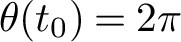 $\theta (t_0)=2\pi $
. This implies that the normal geodesic to
$\theta (t_0)=2\pi $
. This implies that the normal geodesic to $\widetilde v_2$
at
$\widetilde v_2$
at $t_0$
is a straight line parallel to the y-axis. Let
$t_0$
is a straight line parallel to the y-axis. Let $V\subset \mathbb {H}^2$
be the domain enclosed by this line together with an arc of
$V\subset \mathbb {H}^2$
be the domain enclosed by this line together with an arc of $\widetilde v_2$
(see Figure 5, right). Note that V has two interior angles
$\widetilde v_2$
(see Figure 5, right). Note that V has two interior angles $\alpha \in (0,\pi )$
and
$\alpha \in (0,\pi )$
and $\frac {\pi }{2}$
, plus
$\frac {\pi }{2}$
, plus $\widetilde v_2$
is convex toward V. Reasoning as in formula (3.6), we get the same contradiction
$\widetilde v_2$
is convex toward V. Reasoning as in formula (3.6), we get the same contradiction $0>-\operatorname {\mathrm {area}}(V)>\frac {\pi }{2}-\varphi _0$
, which finishes the proof of (a).
$0>-\operatorname {\mathrm {area}}(V)>\frac {\pi }{2}-\varphi _0$
, which finishes the proof of (a).
As for (b), if $\gamma $
intersects the y-axis with angle
$\gamma $
intersects the y-axis with angle $\delta $
, then there is a region
$\delta $
, then there is a region $W\subset \mathbb {H}^2$
bounded by
$W\subset \mathbb {H}^2$
bounded by $\gamma $
,
$\gamma $
, $\widetilde v_2$
, and the y-axis. The Gauss–Bonnet formula, in the same fashion as in formula (3.6), gives the inequality
$\widetilde v_2$
, and the y-axis. The Gauss–Bonnet formula, in the same fashion as in formula (3.6), gives the inequality $0>-\operatorname {\mathrm {area}}(W)>\delta -\varphi _0$
, which is equivalent to
$0>-\operatorname {\mathrm {area}}(W)>\delta -\varphi _0$
, which is equivalent to $\delta <\varphi _0$
. The equality
$\delta <\varphi _0$
. The equality $\mathcal P_2(a,\varphi ,f(a,\varphi ))=\cos (\delta )$
was given in equation (3.3).
$\mathcal P_2(a,\varphi ,f(a,\varphi ))=\cos (\delta )$
was given in equation (3.3).
We will now discuss (c) and (d). Note that $\gamma (\pi )$
has negative first coordinate by the foregoing analysis, so
$\gamma (\pi )$
has negative first coordinate by the foregoing analysis, so $\gamma $
intersects the y-axis if and only the first coordinate of
$\gamma $
intersects the y-axis if and only the first coordinate of
 $$ \begin{align} \gamma(0)=\left(x_0-y_0\frac{1+\cos(\theta_0)}{\sin(\theta_0)},0\right) \end{align} $$
is positive (here, $\sin (\theta _0)<0$
because
$\sin (\theta _0)<0$
because $\pi <\theta _0<2\pi $
). If there exists
$\pi <\theta _0<2\pi $
). If there exists $\delta \in (0,\varphi _0)$
such that
$\delta \in (0,\varphi _0)$
such that $\mathcal P_2(a,\varphi _0,f(a,\varphi _0))=\frac {x_0\sin \left (\theta _0\right )}{y_0}-\cos (\theta _0)=\cos (\delta )\in (0,1)$
, then the first coordinate in equation (3.7) is positive, and it follows from (b) that the angle at the intersection is precisely
$\mathcal P_2(a,\varphi _0,f(a,\varphi _0))=\frac {x_0\sin \left (\theta _0\right )}{y_0}-\cos (\theta _0)=\cos (\delta )\in (0,1)$
, then the first coordinate in equation (3.7) is positive, and it follows from (b) that the angle at the intersection is precisely $\delta $
. If
$\delta $
. If $\mathcal P_2(a,\varphi _0,f(a,\varphi _0))=1$
, then the first coordinate of equation (3.7) vanishes, so
$\mathcal P_2(a,\varphi _0,f(a,\varphi _0))=1$
, then the first coordinate of equation (3.7) vanishes, so $\gamma $
and the y-axis are asymptotic at the ideal point
$\gamma $
and the y-axis are asymptotic at the ideal point $(0,0)$
.
$(0,0)$
.
To finish the proof, let us analyze the limits. Integrating from $0$
to b the identity
$0$
to b the identity $\theta '=\psi '-\cos (\theta )$
in Lemma 1 (applied to
$\theta '=\psi '-\cos (\theta )$
in Lemma 1 (applied to $v_2$
), and taking into account that
$v_2$
), and taking into account that $\theta (b)-\theta (0)=\theta _0-\pi $
and
$\theta (b)-\theta (0)=\theta _0-\pi $
and $\psi (b)-\psi (0)=\varphi _0$
, we get the relation
$\psi (b)-\psi (0)=\varphi _0$
, we get the relation
 $$ \begin{align} \theta_0=\varphi_0+\pi-\int_0^b\cos(\theta(s))\mathrm{d}s. \end{align} $$
In particular, $\theta _0\to \varphi _0+\pi $
and
$\theta _0\to \varphi _0+\pi $
and $(x_0,y_0)\to (0,1)$
as
$(x_0,y_0)\to (0,1)$
as $b\to 0$
(note that the length of
$b\to 0$
(note that the length of $\widetilde v_2$
goes to zero). This implies that the first component of equation (3.7) is positive – that is,
$\widetilde v_2$
goes to zero). This implies that the first component of equation (3.7) is positive – that is, $\gamma (0)$
and
$\gamma (0)$
and $\gamma (\pi )$
lie at distinct sides of the y-axis for b small enough – so
$\gamma (\pi )$
lie at distinct sides of the y-axis for b small enough – so $\gamma $
intersects the positive y-axis at some point. By Lemma 5, if
$\gamma $
intersects the positive y-axis at some point. By Lemma 5, if $a\in (0,a_{\max }(\varphi _0))$
tends to zero, then
$a\in (0,a_{\max }(\varphi _0))$
tends to zero, then $b=f(a,\varphi _0)$
also tends to zero and
$b=f(a,\varphi _0)$
also tends to zero and
 $$ \begin{align*} \lim_{a\to 0}\mathcal P_2(a,\varphi_0,f(a,\varphi_0))=\lim_{a\to 0}\left(\frac{x_0\sin(\theta_0)}{y_0}-\cos(\theta_0)\right)=\cos(\varphi_0). \end{align*} $$
As for the limit $a\to a_{\max }(\varphi _0)$
, let
$a\to a_{\max }(\varphi _0)$
, let $(a_n,\varphi _0)\in \Omega $
be a sequence with
$(a_n,\varphi _0)\in \Omega $
be a sequence with $a_n\to a_{\max }(\varphi _0)$
. Lemma 5 tells us that
$a_n\to a_{\max }(\varphi _0)$
. Lemma 5 tells us that $b_n=f(a_n,\varphi _0)\to +\infty $
, so the surfaces
$b_n=f(a_n,\varphi _0)\to +\infty $
, so the surfaces $\Sigma (a_n,\varphi _0,b_n)$
converge, up to a subsequence and vertical translations (in such a way that
$\Sigma (a_n,\varphi _0,b_n)$
converge, up to a subsequence and vertical translations (in such a way that $h_1$
is a segment at height
$h_1$
is a segment at height $0$
) to a solution
$0$
) to a solution $\Sigma _{\infty }$
of a Jenkins–Serrin problem over an isosceles triangle with values
$\Sigma _{\infty }$
of a Jenkins–Serrin problem over an isosceles triangle with values $0$
along the unequal side and
$0$
along the unequal side and $+\infty $
and
$+\infty $
and $-\infty $
along the other sides. We will denote in the sequel the elements of
$-\infty $
along the other sides. We will denote in the sequel the elements of $\Sigma (a_n,\varphi _0,b_n)$
with a subindex n.
$\Sigma (a_n,\varphi _0,b_n)$
with a subindex n.
-
• If
$l<\infty $
, the conjugate surfaces converge to
$\widetilde \Sigma _{\infty }$
, twice the fundamental piece of a symmetric saddle tower with four ends in the quotient (this conjugate construction is analyzed in [Reference Morabito and Rodríguez16]). If we fix
$\widetilde v_{2n}\subset \mathbb {H}^2\times \{0\}$
, then the curves
$\widetilde {v}_{1n}$
converge to a complete horizontal curve
$\widetilde v_{1\infty }\subset \mathbb {H}^2\times \{-l\}$
(convex toward the exterior of the domain), and the curves
$\widetilde h_{3n}$
tend to an ideal vertical segment
$\widetilde h_{3\infty }$
(see Figure 6). However, we will translate and rotate the surfaces first so that
$\widetilde v_{2n}(0)=(0,1,0)$
and
$\widetilde v_{2n}'(0)=-\partial _x$
in the half-space model in order to analyze the rotation
$\theta _{0n}$
of
$\widetilde v_{2n}'$
with respect to the horocycle foliation (i.e., we adapt the sequence to the setting of Figure 3). This means that a subsequence of
$\Sigma (a_n,\varphi _0,b_n)$
converges no longer to a saddle tower but to a subset of the vertical plane
$x^2+y^2=1$
. Therefore,
$\theta _{0n}\to \frac {3\pi }{2}$
and
$\widetilde v_{2n}(b_n)=(x_{0n},y_{0n})\to (-1,0)$
as
$n\to \infty $
. In view of equation (3.7), we deduce that
$\gamma _n$
does not intersect the positive y-axis for large n, and equation (3.3) implies that
$\mathcal P_2(a_n,\varphi _0,b_n)\to +\infty $
. -
• If
$l=\infty $
, then it is also well known [Reference Morabito and Rodríguez16, Reference Pyo20] that the conjugate surfaces converge to
$\widetilde \Sigma _{\infty }$
, a quarter of a horizontal catenoid when we keep the point
$\widetilde v_{2n}(b_n)$
fixed (and hence the curves
$\widetilde {v}_{1n}$
converge to a complete ideal horizontal geodesic
$\widetilde v_{1\infty }\subset \mathbb {H}^2\times \{-\infty \}$
). However, if we fix
$\widetilde v_{2n}(0)=(0,1,0)$
and
$\widetilde v_{2n}'(0)=-\partial _x$
instead, then a subsequence converges to a subset of the vertical plane
$x^2+y^2=1$
as in the case
$l<\infty $
, so we can reason likewise.


Proof of Theorems 1 and 2
Set $k\geq 3$
. For each
$k\geq 3$
. For each $\frac {\pi }{k}<\varphi <\frac {\pi }{2}$
, Lemma 6 ensures that
$\frac {\pi }{k}<\varphi <\frac {\pi }{2}$
, Lemma 6 ensures that $\mathcal P_2(a,\varphi ,f(a,\varphi ))$
tends to
$\mathcal P_2(a,\varphi ,f(a,\varphi ))$
tends to $\cos (\varphi )$
when
$\cos (\varphi )$
when $a\to 0$
and to
$a\to 0$
and to $+\infty $
when
$+\infty $
when $a\to a_{\max }(\varphi )$
. Since
$a\to a_{\max }(\varphi )$
. Since $\cos (\varphi )<\cos \left (\frac {\pi }{k}\right )$
and
$\cos (\varphi )<\cos \left (\frac {\pi }{k}\right )$
and $\mathcal P_2$
is continuous, there exists some
$\mathcal P_2$
is continuous, there exists some $a_\varphi \in (0,a_{\max }(\varphi ))$
such that
$a_\varphi \in (0,a_{\max }(\varphi ))$
such that $\mathcal P_2(a_\varphi,\varphi ,f(a_\varphi ,\varphi ))=\cos \left (\frac {\pi }{k}\right )$
, though it might not be unique. Therefore, we deduce from Lemma 6(c) that
$\mathcal P_2(a_\varphi,\varphi ,f(a_\varphi ,\varphi ))=\cos \left (\frac {\pi }{k}\right )$
, though it might not be unique. Therefore, we deduce from Lemma 6(c) that $\widetilde \Sigma _\varphi =\widetilde \Sigma \left (a_\varphi ,\varphi ,f(a_\varphi ,\varphi )\right )$
solves both period problems. We will show that
$\widetilde \Sigma _\varphi =\widetilde \Sigma \left (a_\varphi ,\varphi ,f(a_\varphi ,\varphi )\right )$
solves both period problems. We will show that $\Sigma _\varphi =\Sigma \left (a_\varphi ,\varphi ,f(a_\varphi,\varphi )\right )$
, and hence
$\Sigma _\varphi =\Sigma \left (a_\varphi ,\varphi ,f(a_\varphi,\varphi )\right )$
, and hence $\widetilde \Sigma _\varphi $
, has finite total curvature by adapting Collin and Rosenberg’s argument [Reference Collin and Rosenberg2, Remark 7].
$\widetilde \Sigma _\varphi $
, has finite total curvature by adapting Collin and Rosenberg’s argument [Reference Collin and Rosenberg2, Remark 7].
The limit saddle tower ( $l<\infty $
) and catenoid (
$l<\infty $
) and catenoid ( $l=\infty $
) when
$l=\infty $
) when $a\to a_{\max }(\varphi _0)$
. In the proof of Lemma 6, we bring the points at which the arrows aim to a fixed point of
$a\to a_{\max }(\varphi _0)$
. In the proof of Lemma 6, we bring the points at which the arrows aim to a fixed point of $\mathbb H^2$
, so we get vertical planes in the limit (instead of the saddle tower or the catenoid).
$\mathbb H^2$
, so we get vertical planes in the limit (instead of the saddle tower or the catenoid).

To this end, we consider first the case $l=\infty $
. For each
$l=\infty $
. For each $k\in \mathbb {N}$
, let
$k\in \mathbb {N}$
, let $p_1(k)\in \ell _3$
be such that
$p_1(k)\in \ell _3$
be such that $d(p_1(k),p_3)=k$
, and let
$d(p_1(k),p_3)=k$
, and let $\ell _2(k)$
(resp.,
$\ell _2(k)$
(resp., $\ell _3(k)$
) be the geodesic segment joining
$\ell _3(k)$
) be the geodesic segment joining $p_3$
and
$p_3$
and $p_1(k)$
(resp.,
$p_1(k)$
(resp., $p_2$
and
$p_2$
and $p_1(k)$
). For each
$p_1(k)$
). For each $n\in \mathbb {N}$
with
$n\in \mathbb {N}$
with $n\geq f\left (a_\varphi ,\varphi \right )$
, we will consider the Dirichlet problem over the triangle of vertices
$n\geq f\left (a_\varphi ,\varphi \right )$
, we will consider the Dirichlet problem over the triangle of vertices $p_1(k)$
,
$p_1(k)$
, $p_2$
, and
$p_2$
, and $p_3$
with boundary values
$p_3$
with boundary values $f\left (a_\varphi ,\varphi \right )$
on
$f\left (a_\varphi ,\varphi \right )$
on $\ell _1$
, n on
$\ell _1$
, n on $\ell _2(k)$
, and
$\ell _2(k)$
, and $0$
over
$0$
over $\ell _3(k)$
. These conditions span a unique compact minimal disk
$\ell _3(k)$
. These conditions span a unique compact minimal disk $\Sigma _\varphi ^{k,n}$
(with boundary), which is a graph over the interior of the triangle. The surface
$\Sigma _\varphi ^{k,n}$
(with boundary), which is a graph over the interior of the triangle. The surface $\Sigma _\varphi ^{k,n}$
has geodesic boundary and six internal angles, all of them equal to
$\Sigma _\varphi ^{k,n}$
has geodesic boundary and six internal angles, all of them equal to $\frac {\pi }{2}$
, so the Gauss–Bonnet formula gives a total curvature of
$\frac {\pi }{2}$
, so the Gauss–Bonnet formula gives a total curvature of $-\pi $
for
$-\pi $
for $\Sigma _\varphi ^{k,n}$
. As
$\Sigma _\varphi ^{k,n}$
. As $k\to \infty $
, the surfaces
$k\to \infty $
, the surfaces $\Sigma _\varphi ^{k,n}$
converge uniformly on compact subsets (as graphs) to a surface
$\Sigma _\varphi ^{k,n}$
converge uniformly on compact subsets (as graphs) to a surface $\Sigma _\varphi ^n$
over
$\Sigma _\varphi ^n$
over $\Delta $
with boundary values
$\Delta $
with boundary values $f\left (a_\varphi ,\varphi \right )$
over
$f\left (a_\varphi ,\varphi \right )$
over $\ell _1$
, n over
$\ell _1$
, n over $\ell _2$
, and
$\ell _2$
, and $0$
over
$0$
over $\ell _3$
(this convergence is monotonic by the maximum principle). Therefore, Fatou’s lemma implies that the total curvature of
$\ell _3$
(this convergence is monotonic by the maximum principle). Therefore, Fatou’s lemma implies that the total curvature of $\Sigma _\varphi ^{n}$
is at least
$\Sigma _\varphi ^{n}$
is at least $-\pi $
. Finally, we let
$-\pi $
. Finally, we let $n\to \infty $
so the
$n\to \infty $
so the $\Sigma _\varphi ^{n}$
converge (also monotonically) to
$\Sigma _\varphi ^{n}$
converge (also monotonically) to $\Sigma _\varphi $
on compact subsets, and the same argument implies that
$\Sigma _\varphi $
on compact subsets, and the same argument implies that $\Sigma _\varphi $
has finite total curvature at least
$\Sigma _\varphi $
has finite total curvature at least $-\pi $
(note that the Gauss curvature of a minimal surface in
$-\pi $
(note that the Gauss curvature of a minimal surface in $\mathbb {H}^2\times \mathbb {R}$
is nowhere positive, by the Gauss equation). If
$\mathbb {H}^2\times \mathbb {R}$
is nowhere positive, by the Gauss equation). If $l<\infty $
, the same idea works by just truncating at height n (i.e., there is no need to introduce the sequence with index k).
$l<\infty $
, the same idea works by just truncating at height n (i.e., there is no need to introduce the sequence with index k).
By successive mirror symmetries across the planes containing the components of $\partial \widetilde \Sigma _\varphi $
, we get a complete proper Alexandrov-embedded minimal surface
$\partial \widetilde \Sigma _\varphi $
, we get a complete proper Alexandrov-embedded minimal surface $\overline \Sigma _\varphi \subset \mathbb {H}^2\times \mathbb {R}$
.
$\overline \Sigma _\varphi \subset \mathbb {H}^2\times \mathbb {R}$
.
-
• If
$l=\infty $
, then the curve
$\widetilde v_1$
is an ideal horizontal geodesic, and we only need to reflect once about a horizontal plane – that is, the plane containing
$\widetilde v_2$
and
$\widetilde v_3$
. Hence
$\overline \Sigma _\varphi $
consists of
$4k$
copies of
$\widetilde \Sigma _\varphi $
, so the total curvature in this case is not less than
$-4k\pi $
, and [Reference Hauswirth, Menezes and Rodríguez5, Theorem 4] ensures that
$\overline \Sigma _\varphi $
is asymptotic to a certain geodesic polygon at infinity. From the foregoing analysis, each end of
$\overline \Sigma _\varphi $
has asymptotic boundary consisting of four complete ideal geodesics: two horizontal ones obtained from
$\widetilde v_1$
and two vertical ones obtained from
$\widetilde h_2$
. Taking into account that
$\overline \Sigma _\varphi $
has genus
$g=1$
, equation (1.1) (with
$m=k$
) reveals that its total curvature is exactly
$-4k\pi $
.Note that each end of
$\overline \Sigma _\varphi $
is asymptotic to a vertical plane and is contained in four copies of
$\widetilde \Sigma _\varphi $
. We claim that the subset of
$\overline \Sigma _\varphi $
formed by these four copies is a symmetric bigraph, so in particular the end is embedded. This claim follows from the fact that two of these four pieces come from
$\Sigma _\varphi $
and its axially symmetric surface with respect to
$h_2$
, which project to a quadrilateral of
$\mathbb {H}^2$
. Since this quadrilateral is convex, the Krust-type result in [Reference Hauswirth, Sa Earp and Toubiana8] guarantees that the conjugate
$\widetilde \Sigma _\varphi $
and its mirror symmetric surface across
$\widetilde h_3$
form a graph. The other two copies needed to produce the aforesaid bigraph are their symmetric ones with respect to the slice containing
$\widetilde v_2$
and
$\widetilde v_3$
. -
• If
$l<\infty $
, then the composition of the reflections with respect to the horizontal planes containing
$\widetilde v_1$
and
$\widetilde v_3$
is a vertical translation T of length
$2l$
. Thus,
$\overline \Sigma _\varphi $
induces a surface in the quotient of
$\mathbb {H}^2\times \mathbb {R}$
by T with total Gauss curvature at least
$-4k\pi $
, since it consists of
$4k$
pieces isometric to
$\widetilde \Sigma _\varphi $
. This surface has genus
$1$
and
$2k$
ends, so it follows from the main theorem in [Reference Hauswirth and Menezes4] that its total curvature is exactly
$-4k\pi $
. This result also implies that each end of
$\overline \Sigma _\varphi $
is asymptotic to a vertical plane (in the quotient).


Remark 2. It is important to notice that we have not proved the uniqueness of the surface $\Sigma _\varphi $
. This would be automatically true if we could show that the second period
$\Sigma _\varphi $
. This would be automatically true if we could show that the second period $\mathcal P_2(a,\varphi ,f(a,\varphi ))$
is strictly increasing in the parameter a, though a comparison of the surfaces for different values of a seems to be difficult, since we do not even know whether the function f solving the first period problem is monotonic.
$\mathcal P_2(a,\varphi ,f(a,\varphi ))$
is strictly increasing in the parameter a, though a comparison of the surfaces for different values of a seems to be difficult, since we do not even know whether the function f solving the first period problem is monotonic.
As $\varphi $
approaches
$\varphi $
approaches $\frac {\pi }{k}$
, the value
$\frac {\pi }{k}$
, the value $a_\varphi $
solving the two period problems in the proof of Theorems 1 and 2 goes to zero, and the surface
$a_\varphi $
solving the two period problems in the proof of Theorems 1 and 2 goes to zero, and the surface $\widetilde \Sigma _\varphi $
converges, after rescaling, to a genus
$\widetilde \Sigma _\varphi $
converges, after rescaling, to a genus $1$
minimal k-noid in
$1$
minimal k-noid in $\mathbb {R}^3$
(as in Lemma 5(b)). Moreover, when
$\mathbb {R}^3$
(as in Lemma 5(b)). Moreover, when $\varphi $
approaches
$\varphi $
approaches $\frac {\pi }{2}$
, the surface
$\frac {\pi }{2}$
, the surface $\Sigma _\varphi $
converges to an open subset of a helicoid in
$\Sigma _\varphi $
converges to an open subset of a helicoid in $\mathbb {R}^3$
after rescaling, and it follows that the conjugate surfaces
$\mathbb {R}^3$
after rescaling, and it follows that the conjugate surfaces $\widetilde \Sigma _\varphi $
must converge to a quarter of a catenoid in
$\widetilde \Sigma _\varphi $
must converge to a quarter of a catenoid in $\mathbb {R}^3$
(the curve
$\mathbb {R}^3$
(the curve $\widetilde h_1$
converges to half of the neck of such a catenoid).
$\widetilde h_1$
converges to half of the neck of such a catenoid).
3.3 The embeddedness problem
In the proof of Theorems 1 and 2, it is shown that the conjugate piece $\widetilde {\Sigma }_\varphi $
is a graph over the domain
$\widetilde {\Sigma }_\varphi $
is a graph over the domain $\widetilde \Delta \subset \mathbb {H}^2$
. But it could happen that when we reflect
$\widetilde \Delta \subset \mathbb {H}^2$
. But it could happen that when we reflect $\widetilde {\Sigma }_\varphi $
over the vertical plane containing
$\widetilde {\Sigma }_\varphi $
over the vertical plane containing $\widetilde h_1$
, the resulting surface is not embedded, since the reflected curve of
$\widetilde h_1$
, the resulting surface is not embedded, since the reflected curve of $\widetilde v_3$
might intersect
$\widetilde v_3$
might intersect $\widetilde v_3$
. Observe that as the family of examples with k ends converges to a genus
$\widetilde v_3$
. Observe that as the family of examples with k ends converges to a genus $1$
minimal k-noid in
$1$
minimal k-noid in $\mathbb {R}^3$
after blowup (see also [Reference Mazet13]), there do exist nonembedded examples of k-noids and saddle towers with genus
$\mathbb {R}^3$
after blowup (see also [Reference Mazet13]), there do exist nonembedded examples of k-noids and saddle towers with genus $1$
in
$1$
in $\mathbb {H}^2\times \mathbb {R}$
for all
$\mathbb {H}^2\times \mathbb {R}$
for all $k\geq 3$
.
$k\geq 3$
.
Therefore, embeddedness is guaranteed if the extended surface by reflection about the vertical plane containing $\widetilde h_1$
is embedded. The Krust property yields this if the initial surface
$\widetilde h_1$
is embedded. The Krust property yields this if the initial surface $\Sigma _\varphi $
extended by axial symmetry about the geodesic
$\Sigma _\varphi $
extended by axial symmetry about the geodesic $h_1$
is still a graph over a convex domain – that is, if the angle of
$h_1$
is still a graph over a convex domain – that is, if the angle of $\Delta $
at
$\Delta $
at $p_3$
is at most
$p_3$
is at most $\frac {\pi }{2}$
. Elementary hyperbolic geometry shows that this is equivalent to
$\frac {\pi }{2}$
. Elementary hyperbolic geometry shows that this is equivalent to $a\geq a_{\text {emb}}(\varphi )$
, where
$a\geq a_{\text {emb}}(\varphi )$
, where
 $$ \begin{align} a_{\text{emb}}(\varphi)=\operatorname{\mbox{arc sinh}}(\tanh(l)\cot(\varphi)), \end{align} $$
and $\tanh (l)=1$
if
$\tanh (l)=1$
if $l=\infty $
. Hence, the surfaces in Theorems 1 and 2 are properly embedded, provided that
$l=\infty $
. Hence, the surfaces in Theorems 1 and 2 are properly embedded, provided that $a_{\mathrm {emb}}(\varphi )\leq a_\varphi <a_{\max }(\varphi )$
. If
$a_{\mathrm {emb}}(\varphi )\leq a_\varphi <a_{\max }(\varphi )$
. If $l=\infty $
, then
$l=\infty $
, then $a_{\text {emb}}(\varphi )<a_{\max }(\varphi )$
for all
$a_{\text {emb}}(\varphi )<a_{\max }(\varphi )$
for all $\varphi \in \left (0,\frac \pi 2\right )$
; if
$\varphi \in \left (0,\frac \pi 2\right )$
; if $l<\infty $
, there exists
$l<\infty $
, there exists $\varphi _1\in \left (0,\frac \pi 2\right )$
such that
$\varphi _1\in \left (0,\frac \pi 2\right )$
such that $a_{\text {emb}}(\varphi )<a_{\max }(\varphi )$
if and only if
$a_{\text {emb}}(\varphi )<a_{\max }(\varphi )$
if and only if $\varphi \in \left (\varphi _1,\frac \pi 2\right )$
(see Figure 7).
$\varphi \in \left (\varphi _1,\frac \pi 2\right )$
(see Figure 7).
Graphics of the functions $\varphi \mapsto a_{\max }(\varphi )$
and
$\varphi \mapsto a_{\max }(\varphi )$
and $\varphi \mapsto a_{\text {emb}}(\varphi )$
with
$\varphi \mapsto a_{\text {emb}}(\varphi )$
with $l=\infty $
(left) and
$l=\infty $
(left) and $l=1$
(right). In the shaded regions, embeddedness is guaranteed by the Krust property.
$l=1$
(right). In the shaded regions, embeddedness is guaranteed by the Krust property.

However, on the one hand it seems difficult to know whether a value of $a_\varphi $
solving both period problems lies in this interval; on the other hand, embeddedness may occur even if
$a_\varphi $
solving both period problems lies in this interval; on the other hand, embeddedness may occur even if $a\geq a_{\mathrm {emb}}(\varphi )$
does not hold. It is expected that there are always values of
$a\geq a_{\mathrm {emb}}(\varphi )$
does not hold. It is expected that there are always values of $(a,\varphi )$
producing embedded examples solving the two period problems for all
$(a,\varphi )$
producing embedded examples solving the two period problems for all $k\geq 3$
, and it seems reasonable that this occurs when
$k\geq 3$
, and it seems reasonable that this occurs when $\varphi $
becomes close to
$\varphi $
becomes close to $\frac {\pi }{2}$
.
$\frac {\pi }{2}$
.
3.4 Examples with infinitely many ends
Let us tackle the proof of Theorem 3, which is a particular case of the foregoing constructions for $l=\infty $
(the proof can be easily adapted to the case
$l=\infty $
(the proof can be easily adapted to the case $l<\infty $
). Lemma 6 and the continuity of
$l<\infty $
). Lemma 6 and the continuity of $\mathcal P_2$
imply that for all
$\mathcal P_2$
imply that for all $\varphi \in \left (0,\frac \pi 2\right )$
, there are values of
$\varphi \in \left (0,\frac \pi 2\right )$
, there are values of $a\in (0,a_{\max }(\varphi ))$
such that
$a\in (0,a_{\max }(\varphi ))$
such that $\mathcal P_2(a,\varphi ,f(a,\varphi ))$
is either equal to
$\mathcal P_2(a,\varphi ,f(a,\varphi ))$
is either equal to $1$
or greater than
$1$
or greater than $1$
. Let us study these two cases:
$1$
. Let us study these two cases:
-
• If
$\mathcal P_2(a,\varphi ,f(a,\varphi ))=1$
, then
$\widetilde h_1$
and
$\widetilde h_3$
are contained in vertical planes over asymptotic geodesics of
$\mathbb {H}^2$
in view of Lemma 6(d). This means that
$\widetilde \Sigma (a,\varphi ,f(a,\varphi ))$
is contained in the region between these two geodesics – see Figure 8 (center) – and mirror symmetries across the corresponding vertical planes span a group of isometries fixing the common point at infinity. This group contains a discrete group of parabolic translations, and gives rise to the
$1$
-parameter family of parabolic
$\infty $
-noids. -
• The case
$\mathcal P_2(a,\varphi ,f(a,\varphi ))>1$
occurs in an open subset of
$\Omega $
, and gives rise to the
$2$
-parameter family of hyperbolic
$\infty $
-noids. The two geodesics of
$\mathbb {H}^2$
containing the projections of
$\widetilde h_1$
and
$\widetilde h_3$
do not intersect in this case, and successive reflections across their associated vertical planes span a group of isometries containing a discrete group of hyperbolic translations – see Figure 8 (right).



The fundamental domains of a $3$
-noid (left), a parabolic
$3$
-noid (left), a parabolic $\infty $
-noid (middle), and a hyperbolic
$\infty $
-noid (middle), and a hyperbolic $\infty $
-noid (right). Dotted curves represent geodesics containing the projection of
$\infty $
-noid (right). Dotted curves represent geodesics containing the projection of $\widetilde h_1$
and
$\widetilde h_1$
and $\widetilde h_3$
.
$\widetilde h_3$
.

Similar arguments to those in the proof of Theorems 1 and 2 (using the description of periodic surfaces with finite total curvature in [Reference Hauswirth and Menezes4]) show that each end of the constructed surfaces is embedded and has finite total curvature, plus the global surface is Alexandrov-embedded. Observe that in the case of hyperbolic $\infty $
-noids, we can always choose
$\infty $
-noids, we can always choose $a\geq a_{\mathrm {emb}}(\varphi )$
, defined in the previous section, which means that whenever the parameters
$a\geq a_{\mathrm {emb}}(\varphi )$
, defined in the previous section, which means that whenever the parameters $(a,\varphi )$
lie in this open subset of
$(a,\varphi )$
lie in this open subset of $\Omega $
, the reflected surface is a properly embedded hyperbolic
$\Omega $
, the reflected surface is a properly embedded hyperbolic $\infty $
-noid. In the case of parabolic
$\infty $
-noid. In the case of parabolic $\infty $
-noids, we are not able to guarantee global embeddedness.
$\infty $
-noids, we are not able to guarantee global embeddedness.
Acknowledgments
The authors would like to express their gratitude to Magdalena Rodríguez for her valuable comments during the preparation of this manuscript, as well as to the anonymous referee for the thorough revision of the manuscript, which has greatly improved the final presentation. This research was supported by MINECO–FEDER project MTM2017-89677-P and by MCIN/AEI project PID2019-111531GA-I00. The first author is also supported by the FPU programme from MICINN and by MCIN/AEI project PID2020-117868GB-I00. The second author is also supported by EBM/FEDER UJA 2020 project 1380860.
Competing Interests
The authors declare none.


 Open access

