





Introduction
On 11 through 13 July 1954, during an over-snow traverse across the Greenland ice sheet (Schuster, Reference Schuster1954; Fristrup, Reference Fristrup1967), there were above-freezing temperatures and steady, light rain for most of a day in Northwest Greenland at an altitude of 1919 m just below the boundary of the dry-snow facies (Benson, Reference Benson1962, Reference Benson1996). This event introduced notable melt features into the snowpack. Seventy-two years later, following a sequence of well-documented melt events in Greenland in 2002, 2012, 2015, 2019, 2021, 2022 and 2023, we revisit that 1954 event. It provides well-documented, historical evidence of a high-latitude melt event from an earlier era, the result of a large-scale atmospheric circulation feature (an atmospheric river) that is now receiving considerable public attention (e.g. Wedum and others, Reference Wedum, Pettersen, Guy, Gallagher, Shupe and Mattingly2026). Based on the 1954 event, we offer a cautionary note in assessing the extent and intensity of historical melt events in Greenland.
The 1954 event produced significant melt features (ice layers, lenses and percolation columns) in the snow strata at a location where there was usually little or no melt. These icy features persisted and were observed in snow pits the following year, indicating that they were incorporated into the stratigraphic record. We compare and contrast the 1950s pit results with ice core records of melt events, and the satellite record from more-recent melt events. Like the proverbial tale of the blind men and the elephant, we find no single measure that is sufficient to characterize all melt events in Greenland, but combined, they allow the elephant to be described in more realistic detail.
Background
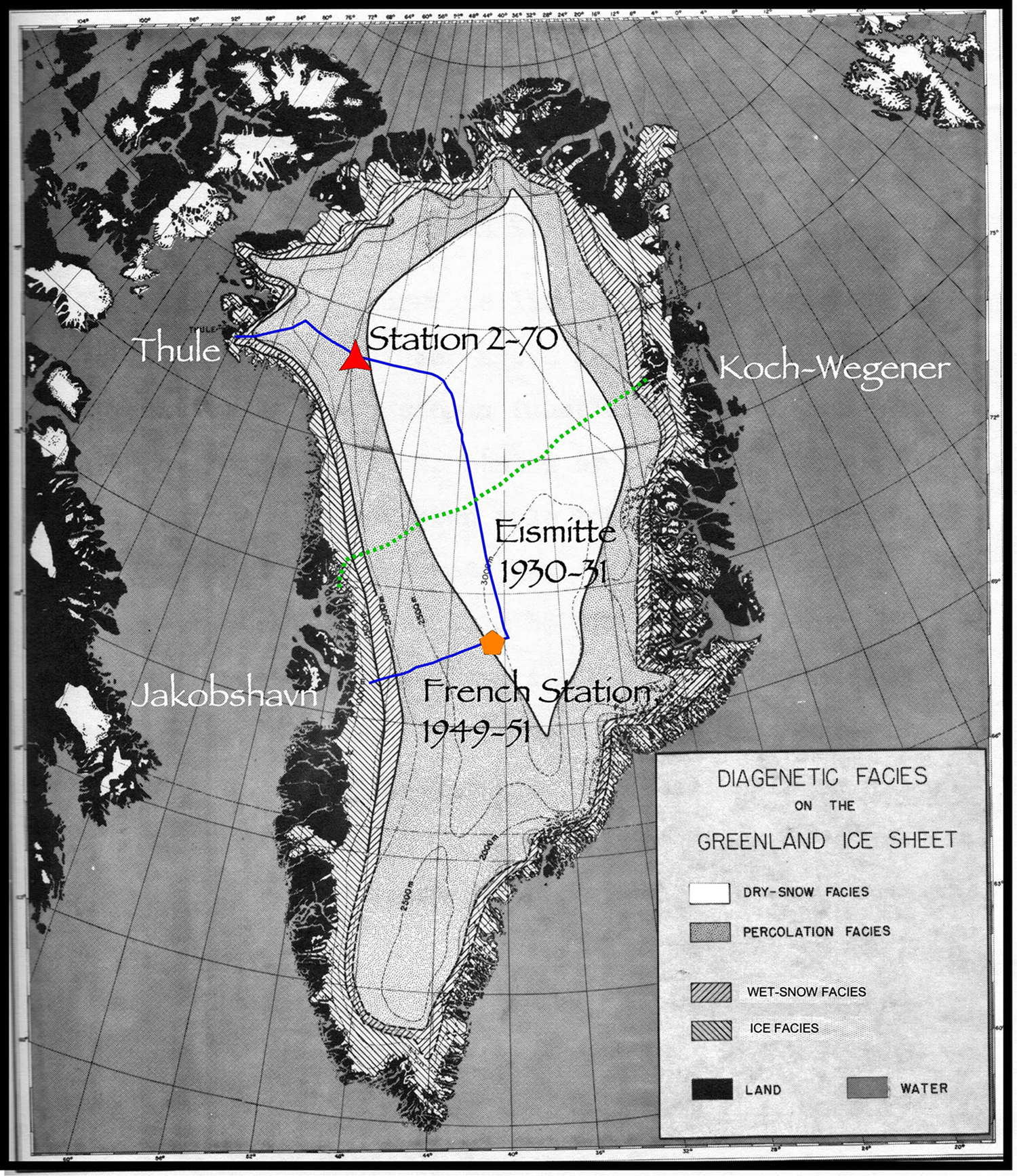
The Danish North Greenland Expedition of 1912–13 was one of the first attempts to determine whether the Greenland ice sheet was growing or shrinking. It was led by Johann Peter Koch and Alfred Wegener, who traversed the ice sheet at 75° N (Ulfarsson and Sigurðsson, Reference Ulfarsson and Sigurðsson2023) (Fig. 1). After World War I, Wegener continued his efforts in 1930–31 during the expedition that established the first winter-over presence at the summit of the ice sheet (Eismitte; cf. Martin-Nielsen, Reference Martin-Nielsen2013), though sadly Wegener himself died during winter resupply efforts (Greene, Reference Greene2015). Three expedition members (Sorge, Georgi and Loewe) spent the winter living in a subterranean snow cave, during which time they dug a 16 m pit in which they were able to identify annual layers in the snow stratigraphy (Sorge, Reference Sorge1933; Loewe, Reference Loewe1935). Further efforts to determine the ice-sheet mass balance were curtailed by World War II. During the war, the Germans established four clandestine weather stations in East Greenland, but Danish military forces, traveling by dogsled, ultimately attacked and eliminated them (Howarth, Reference Howarth2008). Henceforth, the strategic importance of Greenland could not be ignored. In response, the USA established a small weather post at Thule (now called Pituffik), which by 1951 had become a major US Air Force base that remains in operation today (Petersen, Reference Petersen2011).
Distribution of glacier facies on the Greenland ice sheet. The 1952–55 traverse track of this study is shown in blue, with the location of Station 2-70 (red triangle) and the location of Eismitte (orange shape) also shown. The green dashed track is the Koch and Wegener traverse of 1913 (Ulfarsson and Sigurðsson, Reference Ulfarsson and Sigurðsson2023). Jakobshavn is now known by its indigenous name of Ilulissat. From Benson (Reference Benson1962, Reference Benson1996); base figure is in the public domain.

Figure 1 Long description
The map of the Greenland Ice Sheet displays diagenetic facies with distinct zones: dry-snow facies, percolation facies, wet-snow facies and ice facies. These are marked with different patterns. Key locations include Thule, Jakobshavn, Station 2-70, Eismitte and the French Station (1949-51). The 1952-1955 traverse track is shown in blue, while the Koch-Wegener traverse of 1913 is marked with a green dashed line. Station 2-70 is indicated with a red triangle and Eismitte is marked with an orange triangle. The map also includes labels for land and water areas.
With Thule Airbase established and growing, it had become clear for air operations, as well as for fixed radar sites, that far more knowledge of the weather and snow conditions in the interior was needed (Schuster, Reference Schuster1954). Under a US Air Force contract, the American Geographical Society invited the US Army Snow, Ice and Permafrost Research Establishment, now renamed the Cold Regions Research and Engineering Laboratory, to participate in those research efforts. This development led to a series of expeditions (1952–55), led by one of us (C.S.B.), designed to understand the structure, behavior and history of the ice sheet.
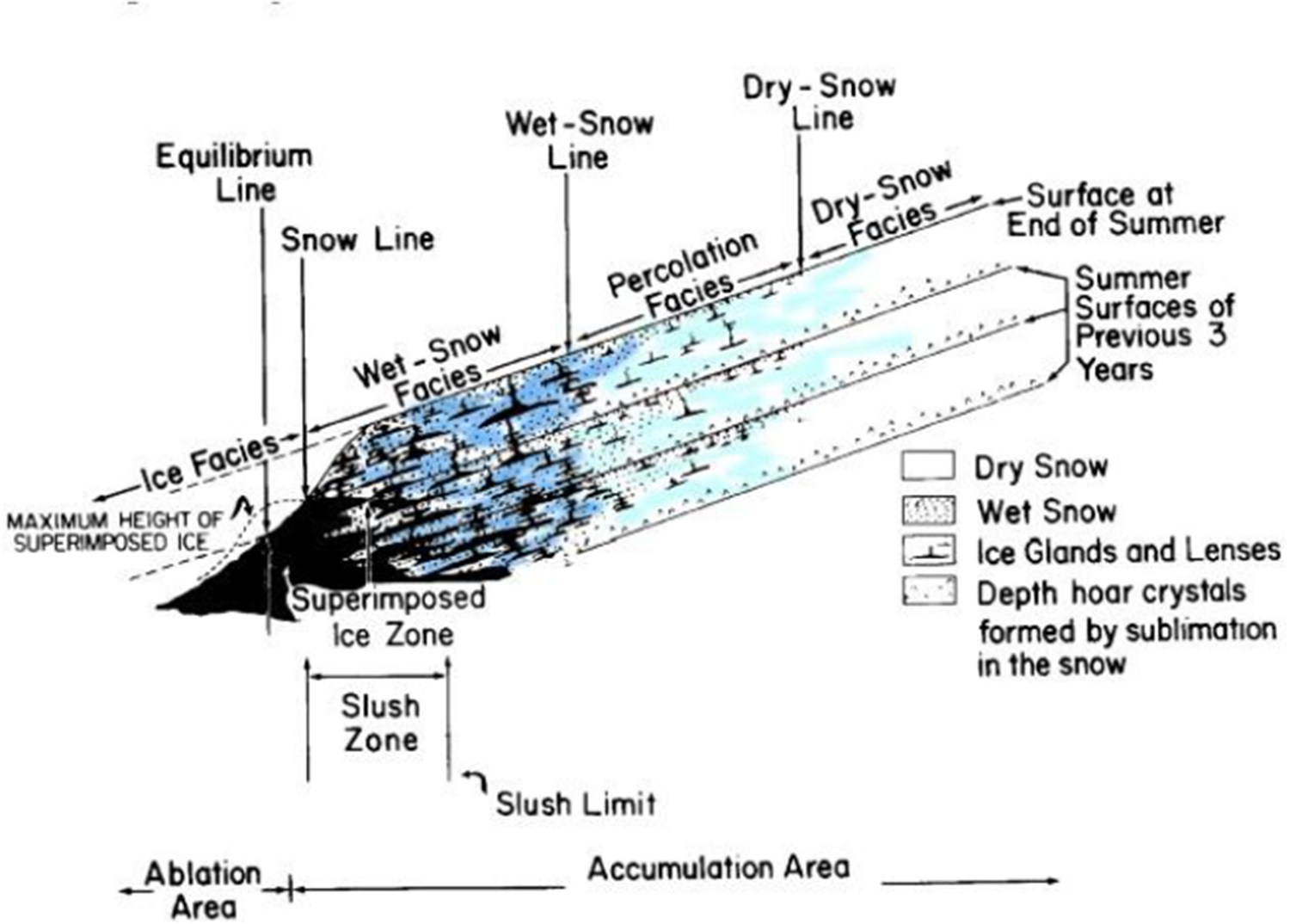
The traverses (Fig. 1) were part of larger efforts to determine accumulation rates on the ice sheet as well as the continuity of snow strata; additionally, geotechnical data on the ice sheet were needed (Sharp, Reference Sharp1951; Bader and others, Reference Bader, Waterhouse, Landauer, Hansen, Bender and Butkovich1955). During the traverses, snow and ice layers were studied at individual sites (hereafter called stations). Shallow cores were taken, and snow pits were dug by members of the expedition, and then the stratigraphy was recorded. This work provided a greatly improved understanding of the processes and stratigraphy of the Greenland ice sheet, and resulted in the development of the groundbreaking glacier facies concept (Figs 1 and 2) (Benson, Reference Benson1962, Reference Benson1996), which has been the framework and underpinning for much of the glaciological work that has taken place in the last seven decades (see, e.g. Jezek and others, Reference Jezek, Gogineni and Shanableh1994; Fahnestock and others, Reference Fahnestock, Bindschadler, Kwok and Jezek1993; Abdalati and Steffen, Reference Abdalati and Steffen1995; Polashenski and others, Reference Polashenski2014).
Schematic illustrating the glacier facies concept. From Benson (Reference Benson1996); base figure is in the public domain.

Figure 2 Long description
The diagram illustrates the glacier facies concept depicting various parts of the ice sheet. At the bottom left, the Ablation Area transitions into the Accumulation Area on the right. The Slush Zone is marked at the bottom, with a Slush Limit line extending horizontally. Above this, the Superimposed Ice Zone is indicated, leading into the Ice Facies. The Equilibrium Line is shown vertically, intersecting the Snow Line, which runs horizontally. The Wet-Snow Line and Dry-Snow Line are also marked, indicating transitions between different snow conditions. The Percolation Facies is located between the Wet-Snow and Dry-Snow Facies. The diagram also shows the Surface at End of Summer and Summer Surfaces of Previous 3 Years, represented by dashed lines. The legend at the bottom right identifies patterns for Dry Snow, Wet Snow, Ice Glands and Lenses and Depth hoar crystals formed by sublimation in the snow.
Results
A rain-on-snow melt event at Station 2-70, 11–14 July 1954
We focus on results from Station 2-70 (Fig. 1), one of a series of pit and core locations along the traverse line. Station 2-70 was located at 77° 05.6′ N, 57° 49.1′ W (1919 m above sea level) just below the boundary between the dry-snow and percolation facies. On 11 July 1954, expedition members noted unusually high temperatures (>0°C) at this location that continued for at least the next 60 h. Intermittent rain occurred on 12 and 13 July, resulting in surface melt that caused severe difficulties in over-snow travel as the expedition moved from Station 2-60 toward Station 2-70. Vehicle tracks on the weasels (small, tracked, over-snow vehicles) carried wet surface snow into the underlying cold snow, resulting in freezing of the tracks. Sled runners had similar problems, and two weasels had to be harnessed together to make progress. Field notes on 12 July (Benson, 1954, unpublished field notes) state: ‘09:45 0°C solid overcast, surface snow very wet, good for making snowballs. Hot, sticky, miserable weather. 12:00 drizzle’. On 13 July, the following was entered, ‘Wet weather, rain and drizzle during night and early morning’.
Analysis of weather records shows that the melt event was generated by an atmospheric river consisting of warm moist air funneled over northern Greenland, as explained in the section below called “Meteorological situation that led to the July 1954 melt event.” The 60+ hour event resulted in ice layers and lenses in the snowpack which were observed in subsequent years after more snow was added to the ice-sheet surface.
Ice core and snow pit evidence of the July 1954 melt event
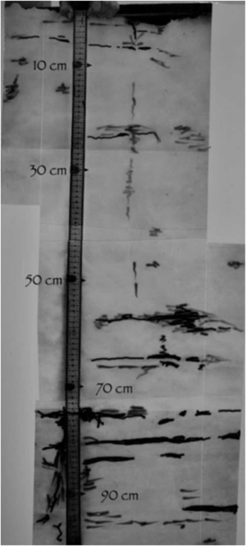
Though the wet weather on 12 and 13 July prevented detailed snow pit and ice core work at Station 2-70, shallow pits were dug on both days to observe the melt action in the upper 2 m of snow (Figs 3 and 4). A wet snow layer 1–2 cm thick formed at the surface everywhere at the station, but there was significant variability at depth. In some of the shallow pits, the snow was wet to a depth of 2 m, while in other locations the snow was wet only in the top few cm with dry snow below (Benson, Reference Benson1962). Between wet and slushy lenses, sections of snow remained between −3 and −10°C. The meltwater descended in isolated channels (percolation columns) that connected perched layers and lenses of wet snow.
The south wall of the pit (see Figure 4) at Station 2-70, showing slush layers and percolation columns on 13 July 1954. We have drawn over the image to enhance clarity. The darker the feature, the more saturated the layer. The ambient snow temperature was −3°C to −10°C between lenses and slush features. From Benson (Reference Benson1996); base figure is in the public domain.

Figure 3 Long description
A tall grayscale rectangular strip with a narrow, dark vertical ruler slightly left of center. To the left of the ruler, black text labels read “10 cm”, “30 cm”, “50 cm”, “70 cm” and “90 cm”, arranged from top to bottom. The background is light gray with multiple dark marks. Near the top, several short, thin horizontal streaks sit to the right of the ruler. Around the middle, a thin vertical dark line runs downward near the center-right, with scattered small dark smudges nearby. Below the “50 cm” label, a thicker cluster of dark, irregular horizontal streaks spans across the right half. Around the “70 cm” label, several long, dark horizontal bands extend across much of the width, with uneven edges and varying thickness. Near the bottom, additional long horizontal dark bands continue, separated by lighter gaps. A light border surrounds the strip.
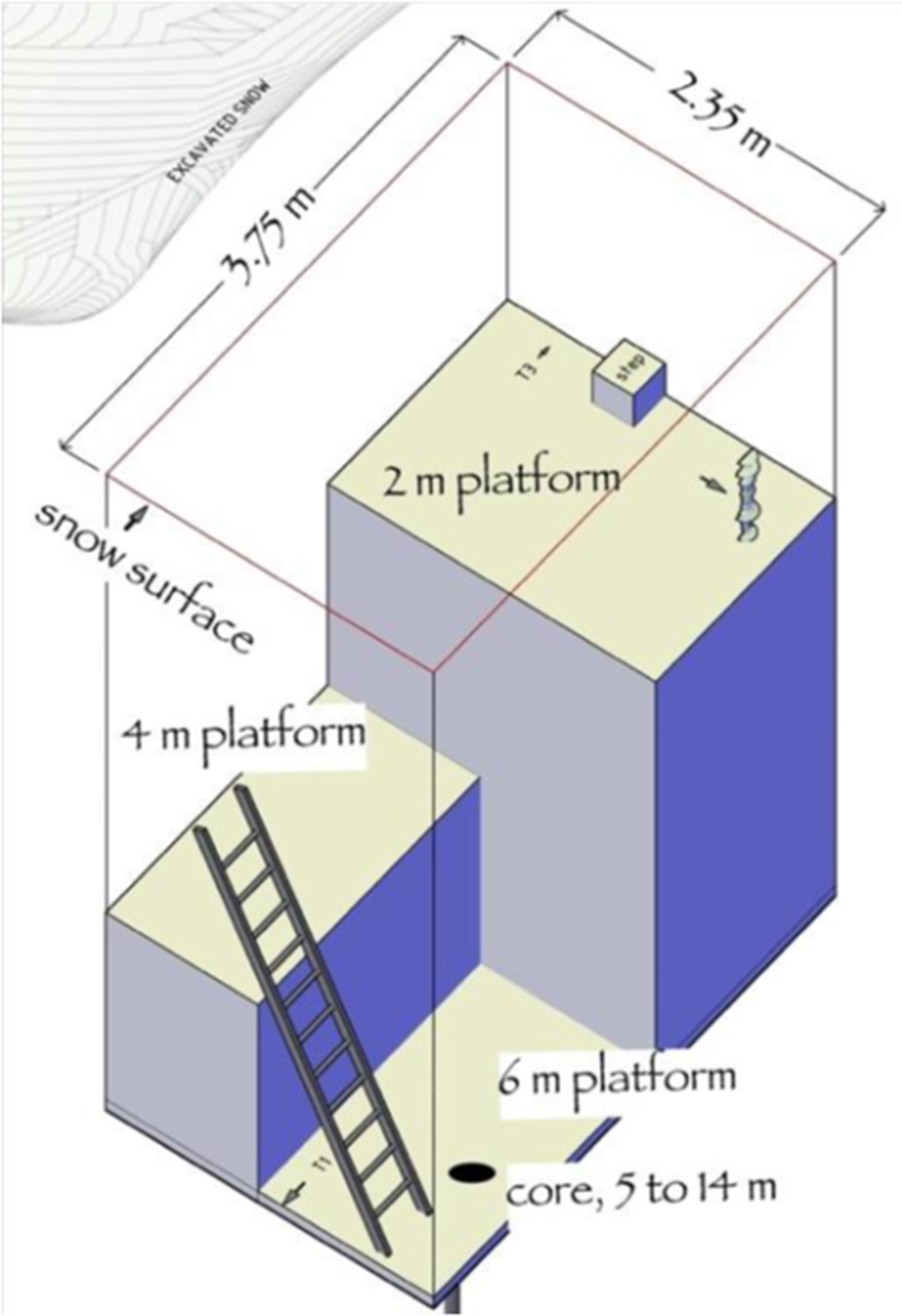
Schematic of a typical pit dug during the 1952–55 traverses (drawing by D. Davis). A total of 42.7 m2 of stratigraphic surface was exposed in each pit, with 12.2 m2 of exposure in the uppermost 1 m of the pit.

Figure 4 Long description
The schematic illustrates a pit structure with three distinct platforms at varying depths. At the top, labeled as the snow surface, the pit measures 3.75 meters in length and 2.35 meters in width. The first platform is positioned at a depth of 2 meters, featuring a small box and a coiled object on its surface. Below this, the second platform is situated at 4 meters, accessible via a ladder extending from the bottom of the pit. The deepest platform is at 6 meters, marked with a label indicating a core depth ranging from 5 to 14 meters. The platforms are enclosed within a rectangular boundary, emphasizing the stratification and depth of the pit. Each platform is distinctly labeled, providing a clear representation of the pit's structure and the snow surface above.
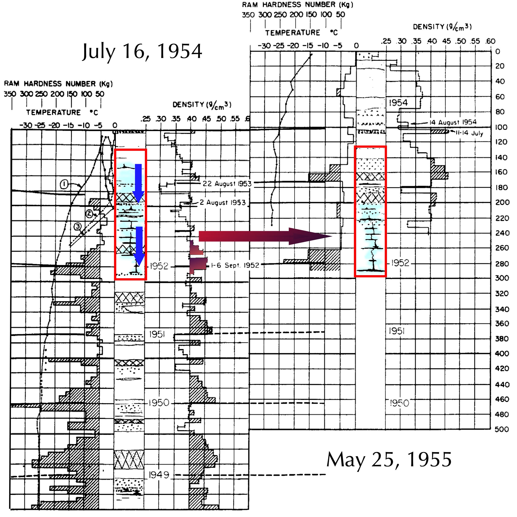
Temperatures cooled on 14 July, enabling pit digging and coring to resume on the 15th at Station 2-70. By that time, surface melt and rain had percolated to a depth of 2.05 m which was well into the snow layers deposited in 1953, where it increased the density of these layers (red histogram area in Fig. 5). The following year, on 25 May 1955, in a large pit adjacent to the 1954 pit, the melt features were found at 2.2–2.9 m depth and therefore could be expected to become a permanent part of the stratigraphic column. Significantly, despite clear melt evidence on the south and east walls of the large pit, there was no indication of the 1954 melt event in the two other walls.
The relationship of the melt features (Figure 3) in 1954 to those observed in 1955. Blue arrows indicate downward percolation; red histogram is the density profile that increased due to percolation. In 1955, the same melt features were observed, but about one meter farther below the surface. From Benson (Reference Benson1996); figure is in the public domain.

Figure 5 Long description
The image shows two scientific profile plots comparing ram hardness, temperature and density versus depth for 16 July 1954 and 25 May 1955. The x-axis for both plots includes RAM HARDNESS NUMBER in kg, TEMPERATURE in degrees Celsius and DENSITY in g per cm superscript 3. The y-axis represents depth from 0 to 500. In the 1954 plot, ram hardness and temperature decrease with depth, while density increases, indicating compaction. A highlighted section from approximately 120 to 280 meters shows melt features with increased density due to percolation. In the 1955 plot, similar melt features appear deeper, from about 140 to 300 meters, suggesting further percolation. The blue arrows indicate downward percolation and the red histogram highlights density changes. The plots illustrate how melt features and density profiles shifted over time, with the 1955 features located about one meter deeper than in 1954.
For context, during the 1955 traverse, a deep core was extracted at Station 2-100 (76° 59.9′ N, 56° 00.8′ W), 48 km east of Station 2-70, capturing snow strata back to 1886 (Bader and others, Reference Bader, Waterhouse, Landauer, Hansen, Bender and Butkovich1955). In this core, evidence of the heaviest melting in 68 years was found to have taken place during the 3 day warm spell (11–13 July) of 1954. The second most intense melt (based on melt layer size) was dated to 1939 or 1940. The core showed more limited melt from 1886 to the early 1920s, then a distinct increase in the number of melt features thereafter.
The two key points concerning the melt features of 1954 are:
1. the features were well developed on the south and east pit faces but completely absent on the north and west pit faces. Assuming percolated water from the melt event extended down to 1 m, then the pit exposed (Fig. 4) ∼12.2 m2 of stratigraphy for inspection, but
2. the wet surface layer was several cm thick everywhere at Station 2-70, ranging from wet to fully saturated, regardless of whether the snow at depth was wet.
Measuring melt intensity on the Greenland ice sheet in the satellite era
The advent of Earth-orbiting satellites has permitted excellent and frequent coverage of the Greenland ice sheet under cloud-free conditions using data from the visible and thermal-infrared (IR) parts of the electromagnetic spectrum. All-weather coverage is also obtained using sensors operating in microwave frequencies. Though useful for quantifying melt extent, visible and thermal IR sensors do not provide explicit details on the intensity of the melt. While even a thin layer of surface melt produces a melt signal in the MODerate-resolution Imaging Spectroradiometer (MODIS) IR and sometimes even in the visible data (Williams et al., Reference Williams, Hall and Benson1991; Hall and others, Reference Hall, Comiso, DiGirolamo, Shuman, Key and Koenig2012), the thickness of that layer cannot be determined. Thin and thick layers produce the same signal. Interpretation of melt intensity has generally required the collection of either snow pit or ice core data.
Passive-microwave signals can reveal important information about an ice sheet, including accumulation rates (Chang and others, Reference Chang, Gloersen, Schmugge, Wilheit and Zwally1976) and melting (Abdalati and Steffen, Reference Abdalati and Steffen1995, Reference Abdalati and Steffen1997). For example, using Scanning Multichannel Microwave Imager data, Abdalati and Steffen (Reference Abdalati and Steffen1997) found that an increasing trend in melt area corresponded with observed increases in coastal temperatures during the period 1979–91, suggesting larger areas of melt might indicate greater melt intensity. More recent studies (e.g. Tedesco, Reference Tedesco2007) have refined those early techniques to map melt on the ice sheet using passive-microwave sensors. It is clear that these passive microwave sensors are sensitive to both surface and subsurface melt, but even now, the sensors still cannot provide an unambiguous assessment of melt intensity, nor can they give a definitive determination of the depth at which the melt features are located.
Satellite radar (active microwave) signals can penetrate into dry snow on an ice sheet. When ice bodies and layers are present, the radar signal reflection from depth (Jezek and others, Reference Jezek, Gogineni and Shanableh1994) provides some information on both extent and melt intensity. However, attributing the source of the radar reflection requires stratigraphic modeling and assumptions about the density profile of the snow, which is largely unknown, making radar assessments of melt intensity across the ice sheet highly uncertain.
Modelers can derive ice-sheet surface mass balance and surface-melt intensity from surface mass-balance models and use ice cores and snow pits to help validate model results (Fettweis and others (Reference Fettweis2020), see their table 3), but there are still large uncertainties, especially in certain parts of the ice sheet. Some of those uncertainties may stem from the inability of ice cores and snow pits to capture all the melt layers that may be present in some parts of the ice sheet in some years of the record.
In short, satellite remote sensing currently provides reliable information on melt extent but not melt intensity for individual melt events. That information still needs to come from ice core and pit stratigraphic data. But there are also uncertainties inherent in relying on ice core and snow pit studies because of the likelihood of underestimating some melt events in some years of the ice core record.
The July 2012 and more-recent surface-melt events
An extreme melt event occurred over 98.6% of the Greenland ice sheet surface on 12–13 July 2012, including at Summit Station (72.58° N, 38.46° W [or 72° 34′ 46.50″ N, 38° 27′ 33.07″ W in DMS]) in the dry-snow facies. The July 2012 event was captured with various types of satellite data: MODIS visible and IR imagery, scatterometer data from the Indian Oceansat-2 satellite, and data from the Special Sensor Microwave Imager/Sounder on a Defense Meteorological Satellite Program satellite (Nghiem and others, Reference Nghiem and Hall2012). The event has been attributed to a ‘heat dome’ (Hanna and others, Reference Hanna2012, Reference Hanna2013) that was parked over central Greenland for the summer.
Though the 2012 event was considered rare at the time, since then, the Greenland ice sheet has experienced several significant surface-melt events that have extended into the dry-snow facies. Melt events extending into the dry-snow facies have also been observed in satellite data in other years, such as 2002 (Hall and others, Reference Hall, Cullather, DiGirolamo, Comiso, Medley and Nowicki2018), 2015, 2019, 2021, 2022 and 2023 (NOAA, 2025). For example, in 2015, an unusual melt event was centered over northern Greenland, driven by a stagnant pressure ridge (Beckman and Winkelmann, Reference Beckmann and Winkelmann2023). During that event, surface-melt extent exceeded 50% of the ice sheet on 4 July 2015 (NOAA, 2025). In 2019, another extreme melt event occurred, with 97% of the ice sheet showing surface melting over 3 days (Tedesco and Fettweis, Reference Tedesco and Fettweis2020). If we use the Abdalati and Steffen (Reference Abdalati and Steffen1997) premise that melt extent is an indicator of intensity, then perhaps we have some indication of what sort of stratigraphic signals these events were producing in the snowpack, but the uncertainty surrounding that assumption, and therefore our understanding of the melt conditions, is large.
Differing synoptic melt conditions: July 1954 vs July 2012
Seventy-two years later, we have been able to determine the meteorological conditions that led to the 1954 melt event at Station 2-70. Here, we contrast those to the conditions that led to the 2012 melt event on the ice sheet.
Atmospheric rivers—narrow corridors of concentrated water vapor that transport moisture from lower latitudes toward the poles—contributed to both events. But the 1954 event was the result of only a narrow atmospheric river (AR) focused on northwestern Greenland, whereas the 2012 melt event involved a much larger weather pattern, including an AR, that produced melt over almost the entire ice-sheet surface. An anomalous ridge of warm air acted as a strong heat dome that stagnated over Greenland in July of 2012 (Hanna and others, Reference Hanna2012).
Any given AR event over Greenland has the potential to produce melt over an area of limited extent, as happened in 1954 at Station 2-70 (Benson, 1954, unpublished field notes). In contrast, a ‘heat dome’ can produce melt over much larger area, as happened spectacularly in 2012, where 98.6% of the ice sheet experienced surface melt (Nghiem et al., Reference Nghiem and Hall2012).
Meteorological situation that led to the July 1954 melt event
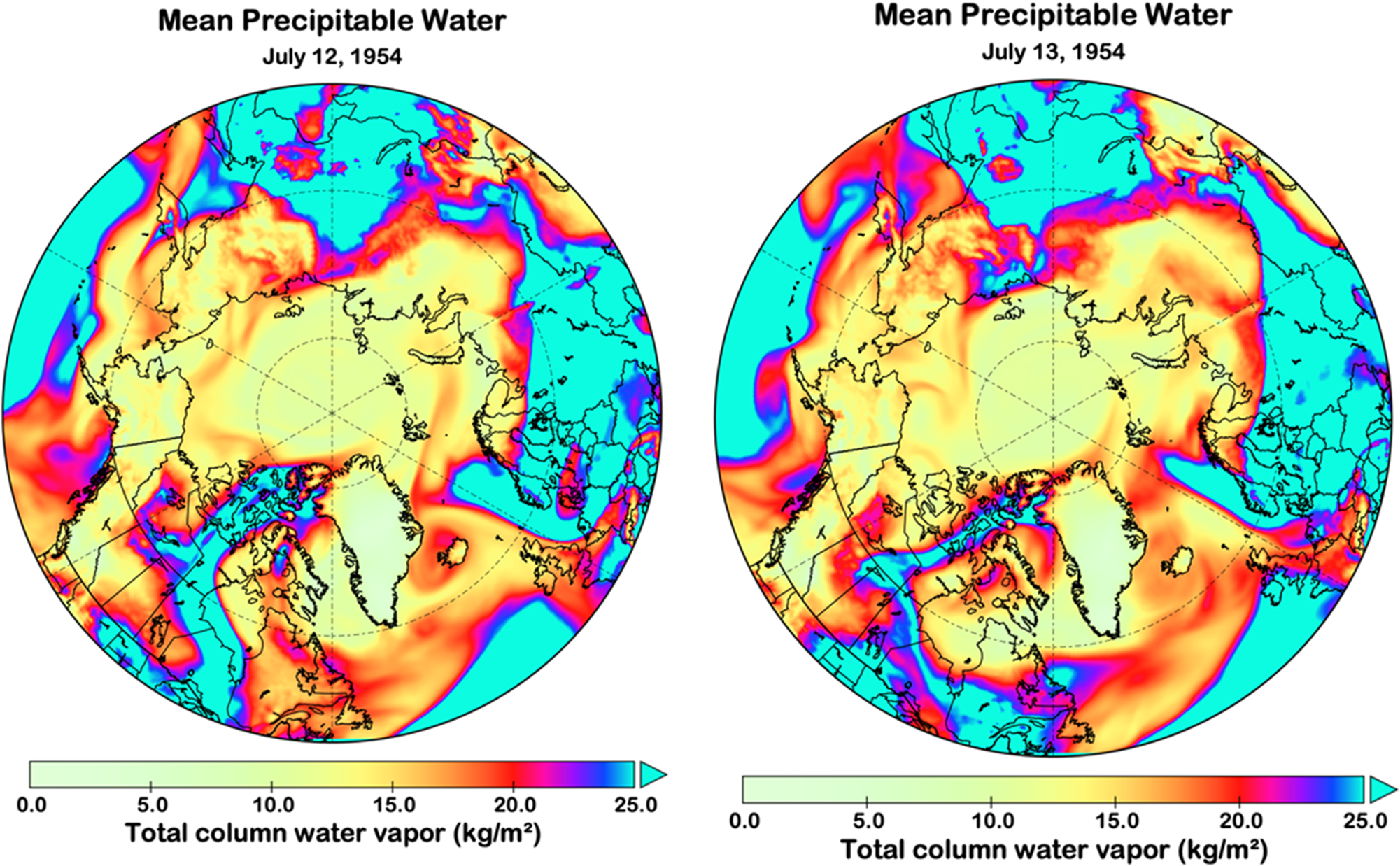
As determined from surface and 500 hPa Northern Hemisphere synoptic weather maps for 11 July 1954 (not shown), an AR that formed over the North American interior near Colorado moved warm, moist air northward to Northwest Greenland, where it caused melting. The mid-troposphere (500 hPa) pattern in the second week of July 1954 reveals two features of importance for this event. Flow around high pressure centered over Hudson Bay transported high-moisture-content air from the Great Lakes region northwestward around the west side of Hudson Bay and then northeast into northeastern Canada. At the same time, low pressure aloft, centered near the North Pole, resulted in increased westerly winds into Northwest Greenland. This combination of the unusually high-moisture-content air (Fig. 6) and the strong westerly winds between the Hudson Bay high and the North Pole low drove the rain on the ice sheet and explains the comparatively limited area that experienced this unusual event. Graphics depicting precipitable water for 11–14 July 1954 show water vapor moving into Northwest Greenland on 12 and 13 July (Fig. 6). By 14 July, the AR had broken down, and conditions on the ice sheet returned to normal.
Mean precipitable water, showing a narrow band of water vapor (an atmospheric river) jetting up into Northwest Greenland on 12–13 July 1954. The data used to develop the figures are derived from the 40 year reanalysis (Kalnay and others, Reference Kalnay1996).

Figure 6 Long description
The image consists of two maps depicting mean precipitable water over the Arctic region on 12 and 13 July 1954. Both maps use a color gradient to represent total column water vapor measured in kg/m². The gradient ranges from 0 to 25.0 kg/m². On 12 July, higher values are concentrated around the central Arctic and parts of northern Europe. On 13 July, the distribution shifts slightly, with increased values extending towards northwest Greenland. The maps illustrate changes in atmospheric moisture over the two days, highlighting areas with significant water vapor presence.
Meteorological situation that led to the July 2012 melt event
For a large part of the summer of 2012, a blocking high-pressure system known as the Greenland Blocking Index (Hanna and others, Reference Hanna2012; Häkkinen and others, Reference Häkkinen, Hall, Shuman, Worthen and DiGirolamo2014) was present in the mid-troposphere over Greenland, advecting warm southerly winds over the western part of the ice sheet and forming a heat dome (Hanna and others, Reference Hanna2012, Reference Hanna2013). From mid-June to early July, there was a succession of warm episodes that increased melting and decreased albedo on the ice sheet (Tedesco and others, Reference Tedesco2013). Around 10 July 2012, an anticyclonic ridge contributed to the melting of most of the winter snow in the ablation facies. This reduced the ice sheet albedo still further. According to Neff and others (Reference Neff, Compo, Ralph and Shupe2014), three main factors contributed to the 12 July 2012 extreme melt: (1) eastward transport of warm air emanating from a heat wave and drought in the mid-North American continent, (2) advection of water vapor in an AR traveling northward over the western Atlantic to western Greenland and (3) disturbances in the polar vortex as measured by excursions of the Arctic Oscillation, creating an opportunity for northward transport of heat and moisture.
Three factors should be taken into account when considering future melt on the Greenland ice sheet; their interaction is anything but simple. The contrast in the spatial scales of the synoptic situations leading to melt for 1954 vs 2012 mirrors the first component: extent. The prior discussion concerning the limitations of remote sensing to measure melt intensity mirrors the second component. The final component, frequency, is revealed primarily through ice cores, as we take up next.
How many melt events? The ice cores record
While the recent melt events have been widespread, as observed using satellite data, one could ask ‘Did they leave lasting stratigraphic signatures?’ which is largely tantamount to asking ‘How intense were these events?’ Both extent and intensity matter when we look to ice core records to assess the frequency of melt events that have been in or near the dry-snow facies of the Greenland ice sheet. The answer is that they have not been rare (Meese and others, Reference Meese1994; Westhoff and others, Reference Westhoff and Sinnl2022). But it is more difficult to know whether they have been localized or widespread.
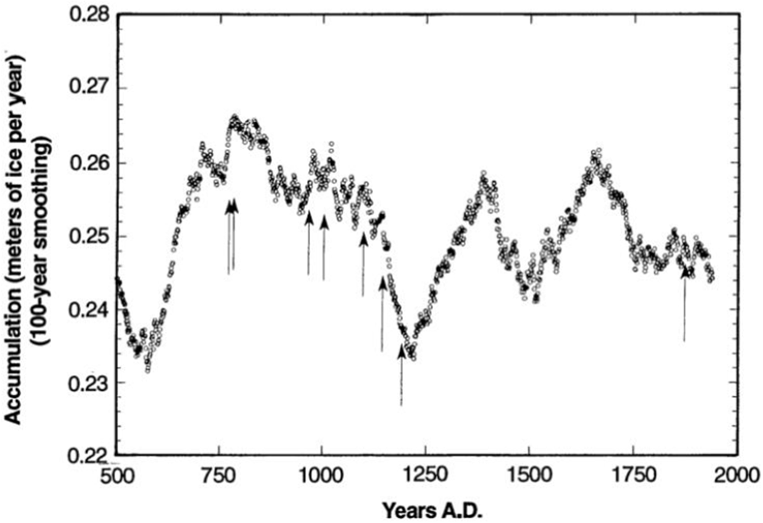
Consider the two ice core records shown in Figs 7 and 8. Both are from the dry-snow facies in Greenland. Meese and others (Reference Meese1994) identified eight distinct melt events during the past 600 years (Fig. 7) in the GISP2 core, with the most recent melt from circa 1870. That suggests a little over one melt event per century. Westhoff and others (Reference Westhoff and Sinnl2022) found between 5 and 22 melt events per century during the last 1000 years in the EastGRIP core (Fig. 8), indicating a melt event every 50–200 years. From these records, we cannot know how extensive those melt events were, except perhaps for the circa 1870 melt in the GISP2 record. This is likely to be the same melt event mapped by Keegan and others (Reference Keegan, Albert, McConnell and Baker2014) using short surface cores, as being a spatially extensive melt event dating to 1889.
Melt events (arrows) identified in the GISP2 core by Meese and others (Reference Meese1994). With permission from the American Association for the Advancement of Science, license date 17 February 2026.

Figure 7 Long description
The graph has a single plotted line with small point markers. The x-axis label is Years A.D. The x-axis ranges from 500 to 2000, with labeled ticks at 500, 750, 1000, 1250, 1500, 1750 and 2000. The y-axis label is Accumulation rate (meters water equivalent per year). The y-axis ranges from 0.22 to 0.28, with labeled ticks at 0.22, 0.23, 0.24, 0.25, 0.26, 0.27 and 0.28. The plotted series starts near 0.24 at about 500. It rises to about 0.26 to 0.27 between about 650 and 800, then declines to about 0.25 by about 1000. It drops to about 0.235 near about 1250. It rises again to about 0.26 to 0.265 between about 1400 and 1600, then varies around about 0.25 to 0.26 from about 1600 to 1900. Near 2000, the values are near about 0.25.
Melt frequency computed from ice layers. Reproduced from Westhoff and others (Reference Westhoff and Sinnl2022) with permission from Copernicus Publications under the Creative Commons Attribution 4.0 License.

Figure 8 Long description
The bar graph displays the number of events and corrections for core breaks over the past 10,000 years. The x-axis represents the number of years before the year 2000, ranging from 0 to 10,000. The y-axis shows events per 100 years, ranging from 0 to 50. The legend identifies three categories: core break correction, melt event (certain and uncertain) and melt event (certain). Bars are stacked vertically to show these categories. Notable peaks occur around 2,000, 4,000 and 6,000 years before the year 2000, with events reaching up to 40 per 100 years. The graph highlights variations in melt events and corrections over time.
Based on the stratigraphic character of the 1954 event (Figs 3 and 4), we suggest that both ice core records cited above underestimate the number of melt events. It is well known that the introduction of meltwater into cold snow produces extremely heterogeneous wetting (Wakahama, Reference Wakahama1968; Marsh and Woo, Reference Marsh and Woo1984; Sturm and Holmgren, Reference Sturm and Holmgren1993), and that this wetting takes place on scales ranging from 0.1 to several meters horizontally, often with unwetted snow between wet areas. Blöschl (Reference Blöschl1999) coined the term ‘support’ for a measurement or observation: it is the physical size of the sample. For any given snow or ice stratum that is penetrated by an ice coring device, the support for identifying melt features is about 0.01 m2. For the snow pits dug during the 1952–55 traverses, the support for similar features was on the order of 12 m2, or about 1200 times larger. Yet even with that much larger sample to canvas, the identification of the 1954 event was only about 50% successful, as half of the pit faces failed to show melt features. It is highly likely that ice cores ‘miss’ melt layers.
Discussion and conclusion
Snow pit measurements, while extremely valuable as stratigraphic records, represent the spatial extent of melt features in Greenland poorly, likely underestimating the extent of melt due to the heterogeneous percolation of water into the snow. However, these in situ sampling measures provide some measure of the intensity of a melt event through the number and thickness of the resulting ice features. For example, Winski and others (Reference Winski and Osterberg2018) used ice cores to count melt layers to develop a 400 year temperature record of Mount Hunter in Central Alaska. If the extent of melt is indeed underestimated in the ice core record, then the regional warming may be greater than they calculated. The spatial extent of surface-melt events can be far better assessed using satellite data, but the satellite data are limited in addressing the intensity of the melt. Ice cores suffer from the same limitations as snow pit measurements, but if allowances are made for the potential of low-bias counting, the cores provide the only means of obtaining the melt frequency going back over substantial periods of time. All three measures and perspectives are necessary to understanding past and present melt events on the ice sheet and for predicting what lies ahead.
In 1954, we witnessed the first documented melt event caused by an atmospheric river pushing warm, moist air into the northwestern part of the Greenland ice sheet. It caused complete and continuous surface melting across a limited area, but even within a single snow pit, the evidence for that melt event could only be detected in two of the four pit walls dug in the following year (Figs 3 and 4). Historical documentation of this unique event highlights the fact that localized melt events within or near the dry-snow facies may have been more common than is reflected in ice-core records. Individual ice cores may not intersect the ice lenses produced by localized melt events. Thus, ice core documentation and analysis of historical melt events in and near the dry-snow facies, and elsewhere on the ice sheet, may underestimate the temporal frequency of melt events.
Acknowledgements
C.S.B. was grateful for his companions during the 1952–55 traverses and for the support of Henri Bader in initiating the work at SIPRE. Logistical field and air support was provided by the US Army. We thank the Benson family for allowing us access to both the field books and diaries from the 1952–55 field seasons. Doug Davis created the CAD drawing in Fig. 4. We also thank Gifford Wong and one anonymous reviewer for their insightful reviews.
Author contributions
C.S.B. led the fieldwork, conceived the idea for this paper and conducted research on the formal analysis. D.K.H., R.T. and M.S. contributed to the formal analysis over a period of many years. R.T. led the meteorological analysis. M.S. led the development and updating of the figures. D.K.H. led the writing of the manuscript, with significant writing also done by R.T. and M.S. Some earlier writing was undertaken by C.S.B.
Dedication
This paper is dedicated to the memory of Carl Benson (Fig. 9), who passed away on 16 January 2026 at the age of 98. Carl was one of the giants in snow and ice research. His varied contributions ranged from the development of the glacier facies concept, to studies of frazil ice formation, to novel studies on ice fog and included some of the first comprehensive studies on the nature and processes shaping Arctic and taiga snow covers. Carl’s passion for glaciology and Arctic research endured throughout his life.
Carl S. Benson, age 23. Photo provided by the Benson family.

While at the Snow, Ice and Permafrost Research Establishment (SIPRE) (now the Cold Regions Research and Engineering Laboratory), Carl led a sequence of traverses across the Greenland ice sheet over a 4 year period (1952–55) using surplus World War II Army track vehicles. Out of this pioneering and painstaking work came the glacier facies concept that underpins most glaciological research today. Carl created maps of the glacier facies and contours of mass balance and temperature in Greenland that, 30 years later, were shown to be remarkably accurate when the ice sheet could be imaged from space.
Carl shared his time unstintingly in mentoring and interacting with a wide circle of colleagues and students. All three coauthors (D.K.H., R.T. and M.S.) feel privileged to have collaborated closely with him over many years, including on this paper.


 Open access

