


1. Introduction and motivation
A robust disaster risk management plan is crucial for the survival and resilience of any nation. A single catastrophic event has the potential to erase decades, if not centuries, of economic progress and threaten livelihoods. According to MunichRe (2021), global losses from natural catastrophes in 2020 amounted to USD 210 billion, marking a significant increase compared to 2019. In the United States, more than 85% of all natural disasters incur costs exceeding a billion dollars, and the cumulative cost of weather and climate disasters since 1980 has surpassed
 $\$$
1.875 trillion (Smith, Reference Smith2021). Furthermore, the ongoing trend of rising temperatures and precipitation driven by climate change is expected to have severe consequences, including the loss of biodiversity, environmental degradation, and increased security and health risks (Linnerooth-Bayer & Hochrainer-Stigler, Reference Linnerooth-Bayer and Hochrainer-Stigler2015; ADB, 2017; Jongman et al., Reference Jongman, Hochrainer-Stigler, Feyen, Aerts, Mechler, Botzen, Bouwer, Pflug, Rojas and Ward2014).
$\$$
1.875 trillion (Smith, Reference Smith2021). Furthermore, the ongoing trend of rising temperatures and precipitation driven by climate change is expected to have severe consequences, including the loss of biodiversity, environmental degradation, and increased security and health risks (Linnerooth-Bayer & Hochrainer-Stigler, Reference Linnerooth-Bayer and Hochrainer-Stigler2015; ADB, 2017; Jongman et al., Reference Jongman, Hochrainer-Stigler, Feyen, Aerts, Mechler, Botzen, Bouwer, Pflug, Rojas and Ward2014).
Disaster Risk Financing (DRF) aims to mitigate the fiscal impacts and economic losses caused by natural hazards, enhancing a country’s financial resilience to such events (WorldBank, 2015). Insufficient protection against disaster risks can result in inadequate funding for rebuilding infrastructure and hinder disaster relief efforts. Conversely, excessive protection may lead to inefficient use of public funds and substantial opportunity costs, limiting a nation’s potential for growth and development. As a result, an increasing number of countries are adopting more proactive and cost-effective approaches to disaster planning to address the extensive human, economic, and fiscal consequences of natural disasters (Mahul et al., Reference Mahul, Signer and Krishna2018). A robust DRF strategy provides governments with rapid access to financial resources during crises, promotes proactive risk management, complements the private insurance sector in transferring catastrophic losses, minimizes humanitarian impacts, and reduces the economic costs of reconstruction (Mahul et al., Reference Mahul, Signer and Krishna2018). However, selecting the appropriate combination and scale of DRF instruments remains a significant challenge. The Global Risk Financing Facility highlights the limited availability of theoretical and empirical studies to guide the effective utilization of risk financing mechanisms (Spencer, Reference Spencer2021).
This paper examines how governments can effectively manage residual financial risksFootnote 1 by employing a combination of DRF instruments, including reserve funds, insurance, contingent credit (CC), and ex-post financing, within the expected utility maximization framework. We incorporate a broad spectrum of real-world considerations commonly used in DRF to derive insights that may not have been previously analyzed or proven. Specifically, we investigate the effects of various factors on the design of a Disaster Fund, including: (i) premium principles, (ii) insurance structures, (iii) risk tolerances and risk horizons, and (iv) the influence of higher-order moments of the loss distribution. The proposed Disaster Fund model is highly adaptable, straightforward to interpret, and accommodates the distinct circumstances of countries with varying degrees of risk aversion, economic and budgetary limitations, and disaster risk profiles.
Our analysis reveals that imposing a Value-at-Risk (VaR) constraint and a Tail VaR (TVaR) constraint yields equivalent outcomes when the quantiles of the VaR and TVaR measures exceed the government’s risk horizon. Under the expected loss premium principle, the Contingent Credit-Insurance (CC-I) layer structure emerges as optimal; however, this may not hold under the standard deviation premium principle. We perform comparative statics to analyze how the optimal mix of DRF instruments adjusts to changes in key inputs, including insurance loadings, interest rates on loans and CC, and risk aversion. Notably, the imposition of a VaR constraint can either increase or decrease the level of insurance coverage, depending on the quantile of the loss distribution relative to the unconstrained optimal parameters. To illustrate the practicality of the Disaster Fund model, we calibrate it using actual flood data from the National Flood Insurance Program (NFIP) in the United States. We explore the optimal mix of DRF instruments and provide visual representations of the parameter space for constructing optimal disaster financing structure under various model specifications.
Given the ambiguity and uncertainty surrounding a government’s true underlying utility function, we avoid deriving closed-form solutions under specific utility functions. While closed-form solutions can often appear elegant and intuitive, they typically require overly restrictive assumptions that omit critical characteristics of real-world scenarios. Instead, the primary contribution of this paper lies in uncovering valuable and previously underexplored insights that are both essential and practical for governments designing DRF funds within an expected utility maximization framework.
1.1 DRF literature review
A review of existing DRF literature reveals an abundance of qualitative studies on DRF adoption but a relative scarcity of quantitative methods and practical guidance for governments on optimally constructing a DRF fund to manage disaster risk (e.g., Kunreuther, Reference Kunreuther1974; Settle, Reference Settle1985; Lewis & Murdock, Reference Lewis and Murdock1996; Harrington, Reference Harrington1997; Weingartner et al., Reference Weingartner, Simonet and Caravani2017; Noy & Edmonds, Reference Noy and Edmonds2019; Oseno & Obiri, Reference Oseno and Obiri2020; Surminski et al., Reference Surminski, Panda and Lambert2019; Ahmed, Reference Ahmed2021). While many studies emphasize the principle of prioritizing risk retention before transferring risk, they often stop short of determining the optimal threshold for retention (Punkdrik, Reference Punkdrik2010; Kashiwagi, Reference Kashiwagi2011; Zelinschi et al., Reference Zelinschi, Domide and Vîrban2013; WorldBank, 2018). These studies frequently rely on arbitrary benchmarks, such as a 1-in-200-year or 1-in-500-year return period, without providing clear justification or assessing the effectiveness and optimality of employing multiple DRF instruments (Vasche & Williams, Reference Vasche and Williams1987; Cornia & Nelson, Reference Cornia and Nelson2003; Barnichon, Reference Barnichon2008; Truong, Reference Truong2021). Moreover, limited research explores the integration of multiple DRF instruments by analyzing diverse insurance structures, real-world constraints, and varied loss profiles to derive optimal strategies for DRF.
The body of quantitative research on the construction of DRF strategies remains limited. In Clarke & Mahul (Reference Clarke and Mahul2011), the authors analyze a range of DRF instruments – savings, loans, CC, and insurance – within a two-period model that maximizes the expected utility of consumption under the expected loss premium principle. They conclude that a layered financing structure is optimal and emphasize the importance of CC. However, their study does not explicitly quantify the optimal allocation of each DRF instrument. Clarke et al. Reference Clarke, Mahul, Poulter and Teh(2017) propose a cost-minimizing strategy for combining disaster risk financial instruments, assuming a risk-neutral government. This framework results in a naturally layered strategy, where DRF instruments are utilized sequentially in order of increasing cost, subject to availability. However, governments are often risk-averse to significant losses, rendering a purely cost-benefit analysis inadequate (Stewart et al., Reference Stewart, Ellingwood and Mueller2011). In contrast to these studies, we advance the literature by determining the optimal allocation of multiple DRF instruments. Our approach incorporates additional practical considerations, including risk aversion, alternative insurance structures, premium principles, VaR and TVaR constraints, risk tolerance, and risk horizon. This comprehensive framework provides a more realistic DRF strategy for addressing the complexities of managing catastrophic risk.
Our paper also connects to the optimal (re)insurance literature. Arrow (Reference Arrow1974) established that the optimal insurance contract under the expected loss premium principle is the excess-of-loss contract, where insurance payouts are triggered only for losses exceeding a specified deductible. The landmark paper by Arrow (Reference Arrow1974) has spurred many extensions such as (1) different risk objective functions and constraints (Huberman et al., Reference Huberman, Mayers and Smith1983; Browne, Reference Browne1995; Huang, Reference Huang2006; Cai and Tan, Reference Cai and Tan2007; Cai et al., Reference Cai, Tan, Weng and Zhang2008; Balbás et al., Reference Balbás, Balbás and Heras2009; Liang & Guo, Reference Liang and Guo2010; Chi & Tan, Reference Chi and Tan2011), (2) different premium principles (Young, Reference Young1999; Chi & Tan, Reference Chi and Tan2013; Liang & Yuen, Reference Liang and Yuen2016a; Chi & Zhou, Reference Chi and Zhou2017; Liang et al., Reference Liang, Wang and Young2022), and (3) different reinsurance structures (Huberman et al., Reference Huberman, Mayers and Smith1983; Zhang et al., Reference Zhang, Zhou and Guo2007; Kaluszka & Okolewski, Reference Kaluszka and Okolewski2008; Liang & Guo, Reference Liang and Guo2011; Ghossoub, Reference Ghossoub2019). Kaluszka & Okolewski (Reference Kaluszka and Okolewski2008) further demonstrated that the excess-of-loss contract remains optimal even when there is an upper bound on insured losses. Our Disaster Fund model can be viewed as a specialized form of the optimal reinsurance problem, where we consider a (1) stepwise increasing cost associated with the use of reserves, (2) proportional and layering insurance structures, (3) expected loss and standard deviation premium principles, (4) VaR and TVaR constraints on terminal fund value, and (5) variable attachment and exhaustion points for both insurance and CC.
We organize the rest of this article as follows. Section 2 introduces the various DRF instruments and key real-world considerations for managing disaster risk, followed by our Disaster Fund methodology and its associated maximization setup. Section 3 presents our theoretical findings and conducts comparative statics. Section 4 provides an empirical study on U.S. flood risk and illustrates the optimal solution to the Disaster Fund model, highlighting the influence of various constraints and assumptions. Finally, Section 5 concludes the paper. Technical details, including proofs and additional figures, are provided in the appendix.
2. Disaster Fund model
2.1 Types of DRF instruments
Following the World Bank classification (Mahul et al., Reference Mahul, Signer and Krishna2018) and a substantial body of DRF literature (Kashiwagi, Reference Kashiwagi2011; Zelinschi et al., Reference Zelinschi, Domide and Vîrban2013; WorldBank, 2018), we group DRF instruments into three broad categories.
-
• Budgetary Measures: These measures refer to the allocation of funds by the government for disaster-related expenditures and are typically risk-retention strategies. These funds can be regular injections (e.g., a proportion of GDP) into reserve funds or reallocations from other programs. For ex-ante reserve funds, a sum of money is set aside for disaster relief, allowing the government to react swiftly when disaster strikes. On the other hand, ex-post borrowing and reallocating funds require no preparatory planning but carry high financial and opportunity costs since interest rates will be extremely high after a disaster, and the government must sacrifice otherwise potentially lucrative and valuable development and improvement projects.
-
• Market-based Instruments: These instruments are usually risk-transfer mechanisms, including insurance and insurance-linked securities such as catastrophic bonds and swaps. Adopting such instruments is imperative for a risk-averse decision-maker since they help remove uncertainty. These instruments transfer risk away from the government to third parties, such as the (re)insurance industry or the catastrophe bond capital market.
-
• Contingent Credit: These instruments are specific to DRF and combine elements of risk retention and risk transfer. An external third party, typically a well-established supranational organizationFootnote 2, agrees to lend a pre-agreed amount of funds to the participating countries in the event of a disaster. The loan typically carries a much lower interest rate compared to ex-post financing. However, countries must determine the maximum drawdown amount and pay a small upfront fee, both at the outset and at recurring intervals during the agreement, based on the maximum available drawdown before a disaster occurs.
Lastly, governments can turn to ex-post borrowing (from the public or other nations) and humanitarian aid (relying on donor countries for assistance) as a last resort to finance disaster losses. However, these ex-post financing options are highly uncertain and costly. The Disaster Fund focuses on the most representative and widely used DRF instruments in each category – reserve fund, insurance, CC, and ex-post borrowing.
2.2 Real-world considerations
In this section, we identify several practical constraints and considerations that governments face in managing disaster risk, which will subsequently be incorporated into the construction of the Disaster Fund model.
Observation 1. (Limited reserves) The government can allocate only a limited amount of funds as reserves for disaster financing.
Funds injections into the Disaster Fund have competing uses and opportunity costs, such as investing in development and improvement projects. Hence, it cannot be inexhaustible, making storing huge amounts of money to self-insure against disaster risk practically infeasible. Political opposition and protests are also likely to occur if a disproportionately large amount of cash is locked away for some future probabilistic event instead of improving citizens’ current welfare. For example, Baratz & Moskowitz (Reference Baratz and Moskowitz1978) note that California’s Proposition 13, which limited tax rates on citizens, was partly motivated by public discontent over a
 $\$$
5 billion surplus held by the government while taxpayers felt overburdened by excessive taxation. Consequently, the limited reserves that the government can accumulate are often insufficient to cover significant disaster losses, requiring the government to explore other funding sources.
$\$$
5 billion surplus held by the government while taxpayers felt overburdened by excessive taxation. Consequently, the limited reserves that the government can accumulate are often insufficient to cover significant disaster losses, requiring the government to explore other funding sources.
Observation 2. (Limited risk horizon) A government will only protect itself from disaster risk up to a certain threshold.
A government typically does not protect itself from the entire spectrum of disaster risk, particularly when the risk involves exceptionally large losses. For example, within the past 10 years (2010–2020), there have been 8,235 emergency declarations and 14,539 major disaster declarations by U.S. states, which are instances where the individual states face disaster damages beyond their planned capability and resources and, thus, request federal assistance. (FEMA, 2023). Similarly, the National Flood Insurance Program (NFIP) in the U.S. relies on federal borrowings to cover extreme flood losses, as its purchase of public reinsurance and issuance of catastrophe bonds only provide coverage up to a certain threshold (Horn, Reference Horn2024). There are several possible explanations for a government to adopt a limited risk horizon. For enormous losses, governments may consider such disasters too unlikely to occur, or they may believe that securing protection against such remote events is not justified given the associated effort and opportunity costs. Budget constraints (insurance premiums covering the whole disaster loss are impractically high) and a myopic mindset (it is highly unlikely for a disaster to occur within the next few years) are common reasons to forsake planning efforts for such massive losses. The scarcity of market participants willing to absorb high-severity, low-likelihood disaster risk further exacerbates the issue. Additionally, moral hazard may play a role, as governments might expect humanitarian aid from other countries or organizations in the event of catastrophic disasters.
Observation 3. (Risk aversion) For potentially monumental losses, governments exhibit risk aversion behavior.
A critical consideration often overlooked in many DRF papers is the government’s risk aversion. Stewart et al. Reference Stewart, Ellingwood and Mueller(2011) suggest that for non-catastrophic events, governments typically adopt a net present value (NPV) approach to evaluate projects, implying risk neutrality. However, this NPV method fails to account for many of the risk-averse actions governments take regarding catastrophic lossesFootnote 3. Kaufman (Reference Kaufman2014) discusses why many governments tend to overlook the risk-reduction benefits of their actions by failing to account for uncertainties, and strongly recommends that policymakers adjust their decision-making processes to include risk-aversion analysis. Harris (Reference Harris2014) further highlights that governments often exhibit risk-neutrality in response to climate events due to political factors. By framing climate change as “unpredictable, unavoidable, or simply natural,” governments may justify their inaction. However, this mindset can be detrimental, as “by the time climate change impacts are bad enough for policymakers to react effectively, it will probably be too late” (Harris, Reference Harris2014). These examples underscore the importance of adopting a utility-based framework in disaster risk management that accounts for the government’s risk aversion.
Observation 4. (Risk tolerance) Governments seek to limit risk exposure.
Governments typically define acceptable risk levels to ensure they can address essential disaster response requirements while maintaining balanced risk exposure. To achieve this, they establish targets based on preferred risk measures, selected to align with specific objectives such as solvency or capital adequacy requirements (Bernard & Tian, Reference Bernard and Tian2009; Chen et al., Reference Chen, Li and Li2010; Melnikov & Smirnov, Reference Melnikov and Smirnov2012). Among these, VaR and TVaRFootnote 4 are the most commonly employed risk measures.
Under the VaR constraint, the government necessitates that the terminal value of the Disaster Fund remains above a pre-determined threshold after a disaster loss at or below the
 $p$
-th percentile if its distribution occurs. For example, insurers under Solvency II must meet a 99.5% VaR requirement (BIS, 2019), while banks under Basel III adhere to a 99.9% VaR standard (EU Commission, 2015). The VaR measure is widely adopted due to its simplicity, interpretability, and ease of communication, making it a popular choice among regulators and financial institutions for quantifying risk.
$p$
-th percentile if its distribution occurs. For example, insurers under Solvency II must meet a 99.5% VaR requirement (BIS, 2019), while banks under Basel III adhere to a 99.9% VaR standard (EU Commission, 2015). The VaR measure is widely adopted due to its simplicity, interpretability, and ease of communication, making it a popular choice among regulators and financial institutions for quantifying risk.
Conversely, a TVaR constraint limits exposure to extreme disaster losses by ensuring that the conditional expected terminal value of the Disaster Fund in the tail of the distribution remains above a specified threshold. The TVaR measure is highly relevant for DRF, given that disaster losses are often characterized by high skewness and fat tails. Unlike VaR, which only considers losses up to a certain quantile, TVaR accounts for the average severity of losses beyond this threshold, addressing the limitations of VaR in ignoring extreme tail risks. In the financial sector, the significance of TVaR has been increasingly recognized. Basel IV, implemented starting in 2023, mandates the use of TVaR at the 97.5% confidence level as a primary risk measure, underscoring its effectiveness in providing a comprehensive assessment of extreme risk scenarios (pwc, 2016; FTSE, 2022).
Observation 5. (Insurance structure) The two primary types of insurance coverage are excess-of-loss and proportional structures.
Under many optimal insurance problems, the excess-of-loss indemnity structure often emerges as the optimal structure (see, e.g., Arrow, Reference Arrow1974; Denuit & Vermandele, Reference Denuit and Vermandele1998; Kaluszka & Okolewski, Reference Kaluszka and Okolewski2008). The superiority of the excess-of-loss structure arises from its flexibility to allow the policyholder to self-insure and avoid paying insurance loading for low-severity risk while removing high-severity risk, which is more volatile and uncertain, especially when the policyholder is highly risk-averse relative to the insurer.
However, practical considerations may render the proportional insurance structure preferable in certain contexts. For example, Huberman et al. Reference Huberman, Mayers and Smith(1983) argue that deductible contracts are suboptimal when there exist economies of scale in cost management. Lampaert & Walhin (Reference Lampaert and Walhin2006) highlight that proportional insurance can reduce moral hazard and is simpler to price. Additionally, Raviv (Reference Raviv1992) shows that co-insurance arrangements are optimal when insurers exhibit risk aversion or when insurance costs are non-linear. Similarly, our study’s inclusion of numerous real-world considerations in designing the DRF fund may suggest that the excess-of-loss structure is not necessarily optimal. These considerations introduce complexities that can alter the balance of costs and benefits associated with each insurance structure, potentially favoring the proportional structure under specific circumstances.
Observation 6. (Insurance premium) Insurers set premium loadings based on both the expectation and the volatility of the claim payments.
Variability-based premium principles have been extensively explored in the actuarial literature (see, e.g., Kaluszka, Reference Kaluszka2001; Chi, Reference Chi2012; Liang and Yuen, Reference Liang and Yuen2016b). Notably, Zeng & Luo (Reference Zeng and Luo2013) demonstrate that under the standard deviation or variance premium principle, the proportional insurance structure emerges as optimal. Furthermore, Landsman & Sherris (Reference Landsman and Sherris2001) critique that the expected value principle does not preserve a consistent risk ordering, as it neglects the variability of risks by assuming that two risks are indifferent as long as their expected payouts are equivalent – an oversight that is particularly significant in catastrophic loss scenarios. Lane & Mahul (Reference Lane and Mahul2008) also provide empirical evidence showing that catastrophe bonds are priced with up to a 44.9% premium loading on the standard deviation of losses, in addition to accounting for expected loss. In this paper, we adopt a hybrid approach that combines both the expected loss and standard deviation premium principles, ensuring a more realistic pricing mechanism. Premium loadings on expected loss help cover claims payouts, administrative charges, and profit margins of the insurer, while loadings on the standard deviation of losses compensate for the high uncertainty and risk borne by the insurer in relation to non-catastrophic risks.
2.3 Disaster Fund
Consider a government seeking to establish a Disaster Fund for effective disaster risk management. The design of the Disaster Fund must incorporate the various instruments discussed in Section 2.1, while also adhering to the constraints and considerations outlined in Section 2.2.
Firstly, since the reserve fund is the most cost-effective form of capital, the government will prioritize its use. Therefore, for low-severity losses up to a certain endogenous threshold
 $L$
, the government will opt to use the reserve funds over other instruments. This approach is akin to self-insuring against the first portion of disaster risk from
$L$
, the government will opt to use the reserve funds over other instruments. This approach is akin to self-insuring against the first portion of disaster risk from
 $0$
to
$0$
to
 $L$
. To integrate Observation1 into the Disaster Fund model, we impose a cap on the availability of the reserve fund, denoted as
$L$
. To integrate Observation1 into the Disaster Fund model, we impose a cap on the availability of the reserve fund, denoted as
 $k_L$
, which is exogenously determined. Once the reserve fund is depleted, the government must then rely on alternative methods to finance the remaining lossesFootnote 5.
$k_L$
, which is exogenously determined. Once the reserve fund is depleted, the government must then rely on alternative methods to finance the remaining lossesFootnote 5.
From Observation2, there exists an upper threshold loss amount
 $U$
such that losses above
$U$
such that losses above
 $U$
beyond which the government does not plan in advance to cover disaster losses, as these losses exceed its defined risk horizon. For losses surpassing
$U$
beyond which the government does not plan in advance to cover disaster losses, as these losses exceed its defined risk horizon. For losses surpassing
 $U$
, the government will resort to ex-post financing methods, such as borrowing or reallocating budget from other sources, since ex-post financing generally comes with extremely high interest rates and significant opportunity costs, making it a last resort option after all ex-ante alternatives have been exhausted. Furthermore, we introduce an exogenous upper bound
$U$
, the government will resort to ex-post financing methods, such as borrowing or reallocating budget from other sources, since ex-post financing generally comes with extremely high interest rates and significant opportunity costs, making it a last resort option after all ex-ante alternatives have been exhausted. Furthermore, we introduce an exogenous upper bound
 $k_U$
for
$k_U$
for
 $U$
where the government will cease arranging additional DRF instruments. This limit could be driven by external factors, such as the unavailability of insurance markets or CC facilities willing to cover extremely severe losses.
$U$
where the government will cease arranging additional DRF instruments. This limit could be driven by external factors, such as the unavailability of insurance markets or CC facilities willing to cover extremely severe losses.
Lastly, for the remaining losses of moderate loss severity between
 $L$
and
$L$
and
 $U$
, the government will adopt a combination of risk retention and risk transfer strategies – specifically, insurance and CC – to cover disaster losses. This approach aligns with the World Bank’s recommended tiers of risk management: (i) self-retention to finance small but recurrent disasters, (ii) CC mechanisms for less frequent but more severe events, and (iii) disaster risk transfer, such as insurance, to cover major natural disasters (GFDRR, 2015). Our primary focus will be on this layer of risk management. The left diagram of Fig. 1 summarizes the key elements of the model discussed thus far.
$U$
, the government will adopt a combination of risk retention and risk transfer strategies – specifically, insurance and CC – to cover disaster losses. This approach aligns with the World Bank’s recommended tiers of risk management: (i) self-retention to finance small but recurrent disasters, (ii) CC mechanisms for less frequent but more severe events, and (iii) disaster risk transfer, such as insurance, to cover major natural disasters (GFDRR, 2015). Our primary focus will be on this layer of risk management. The left diagram of Fig. 1 summarizes the key elements of the model discussed thus far.
The Disaster Fund model. We consider two strategies, which consist of three distinct layers for losses with various severities, along with the parameters to optimize.

Let
-
•
 $R_0 \in \mathbb{R}$
denotes the initial wealth allocated to the fund by the government,
$R_0 \in \mathbb{R}$
denotes the initial wealth allocated to the fund by the government, -
•
$F_{CC},r_{CC},r_e \geq 0$
denote the per-unit upfront administrative charge of CCFootnote 6, rate of interest for CC, and the rate of interest for ex-post borrowing, respectively, -
•
$X$
denotes a continuousFootnote 7, non-negative random variable modeling the disaster loss with a cumulative distribution function
$F_X(x)$
and a density function
$f_X(x)$
, -
•
$Y_I(X),Y_{CC}(X),Y_e(X) \geq 0$
denote the cashflows from insurance claims, CC, and ex-post financing, respectively, and -
•
$C_I, C_{CC} \geq 0$
denote the insurance premium and upfront cost for arranging CC, respectively.


To establish the Disaster Fund, the government determines the allocation of each DRF instrument to adopt across various loss severities, governed by endogenous variables
 $L,M,U$
for the CC-I layer structure and
$L,M,U$
for the CC-I layer structure and
 $L,\alpha ,U$
for the proportional structure. At the fund’s inception, the government pays the insurance premium
$L,\alpha ,U$
for the proportional structure. At the fund’s inception, the government pays the insurance premium
 $C_I$
and the upfront cost of the CC
$C_I$
and the upfront cost of the CC
 $C_{CC}$
. Upon the occurrence of a disaster event, the government raises the realized disaster loss amount
$C_{CC}$
. Upon the occurrence of a disaster event, the government raises the realized disaster loss amount
 $X$
in full according to the predetermined Disaster Fund strategy. The realized loss will first be raised through the reserve fund
$X$
in full according to the predetermined Disaster Fund strategy. The realized loss will first be raised through the reserve fund
 $L$
, followed by a mix of insurance payout
$L$
, followed by a mix of insurance payout
 $Y_I(X)$
and CC
$Y_I(X)$
and CC
 $Y_{CC}(X)$
if the reserve fund is insufficient to cover the entire disaster loss, and finally, the government resorts to ex-post financing
$Y_{CC}(X)$
if the reserve fund is insufficient to cover the entire disaster loss, and finally, the government resorts to ex-post financing
 $Y_{e}(X)$
as a last resort. Subsequently, if CC facilities or ex-post financing are utilized, the government is obligated to repay the loans with interest charged at
$Y_{e}(X)$
as a last resort. Subsequently, if CC facilities or ex-post financing are utilized, the government is obligated to repay the loans with interest charged at
 $r_{CC}$
and
$r_{CC}$
and
 $r_e$
, respectively. Thus, the terminal Disaster Fund value after disaster occurrence and loan repayments is
$r_e$
, respectively. Thus, the terminal Disaster Fund value after disaster occurrence and loan repayments is
 \begin{align} R_1(X) &= R_0 - C_I - C_{CC} \kern7pt\qquad\qquad\qquad\qquad\qquad\qquad \text{(fund initiation)} \\ &\quad -X+Y_I(X)+Y_{CC}(X)+Y_e(X) \qquad \qquad \text{ (disaster occurrence) } \nonumber \\ & \quad - (1+r_{CC})Y_{CC}(X) - (1+r_e)Y_e(X). \qquad \qquad \text{ (loan repayment) }\nonumber \end{align}
 \begin{align} &= R_0 - C_I - C_{CC} - X + Y_I(X) \\ & \quad - r_{CC} Y_{CC}(X) - r_{e} Y_{e}(X).\nonumber \end{align}
Equation (1) groups cashflows occurring at different points in time. In contrast, disregarding the terms
 $C_{\text{CC}}$
,
$C_{\text{CC}}$
,
 $Y_{\text{CC}}(X)$
, and
$Y_{\text{CC}}(X)$
, and
 $Y_{\text{e}}(X)$
, Equation (2) coincides with the utility maximization problem of the renowned Arrow (Reference Arrow1974) model. However, disaster losses are often extraordinarily large, making it impractical for governments to self-retain risk, even when this may be the utility-maximizing solution. Consequently, governments must resort to borrowing to manage retained risk, incurring additional interest payments compared to the zero interest cost associated with using initial wealth. For each DRF instrument, a marginal unit of disaster loss is financed by
$Y_{\text{e}}(X)$
, Equation (2) coincides with the utility maximization problem of the renowned Arrow (Reference Arrow1974) model. However, disaster losses are often extraordinarily large, making it impractical for governments to self-retain risk, even when this may be the utility-maximizing solution. Consequently, governments must resort to borrowing to manage retained risk, incurring additional interest payments compared to the zero interest cost associated with using initial wealth. For each DRF instrument, a marginal unit of disaster loss is financed by
-
(i) one dollar of initial wealth,
-
(ii) one dollar of insurance payoff,
-
(iii)
$(1+r_{CC})$
dollars from a CC loan, or -
(iv)
$(1+r_{e})$
dollars from an ex-post loan.


In an unconstrained scenario, option (i) is the most cost-effective, followed by (iii), with (iv) being the least favorable. Consequently, the government will naturally prioritize funding disaster losses using its own wealth, then CC, and finally ex-post borrowing. To reflect real-world constraints, the limited reserve constraint caps the wealth allocated as a reserve at
 $k_L$
, and the limited risk horizon constraint imposes an upper limit
$k_L$
, and the limited risk horizon constraint imposes an upper limit
 $k_U$
on the combined use of CC and insurance. Any self-retained risk exceeding
$k_U$
on the combined use of CC and insurance. Any self-retained risk exceeding
 $k_L$
must be financed through CC, and losses beyond
$k_L$
must be financed through CC, and losses beyond
 $k_U$
necessitate ex-post financing.
$k_U$
necessitate ex-post financing.
In summary, our model is a one-period static framework based on Arrow (Reference Arrow1974)’s setup, with modifications tailored to the context of disaster losses. Specifically, self-retention becomes costly beyond a certain threshold as borrowing is required. The rising cost of capital discourages self-retention and promotes the purchase of insurance.
We assume that initial wealth is not a limiting constraint, meaning the initial fund is sufficiently large to cover at least the reserve fund, the insurance premium, and the CC upfront fee, such that
 $R_0 \gt L + C_I + C_{CC}$
. In practice, loan repayments often occur over future periods and may extend across multiple years. However, for analytical convenience, we simplify the model into a single-period framework. Heuristically, the interest rates
$R_0 \gt L + C_I + C_{CC}$
. In practice, loan repayments often occur over future periods and may extend across multiple years. However, for analytical convenience, we simplify the model into a single-period framework. Heuristically, the interest rates
 $r_{CC}$
and
$r_{CC}$
and
 $r_e$
can be interpreted as adjusted rates, reflecting the net impact of the discounted time value of money and the potential investment returns of the fund over the repayment period.
$r_e$
can be interpreted as adjusted rates, reflecting the net impact of the discounted time value of money and the potential investment returns of the fund over the repayment period.
2.4 Insurance structures and premium principles
Based on Observation5, we consider two distinct structures for combining insurance and CC to address mid-severity losses between
 $L$
and
$L$
and
 $U$
. Under the excess-of-loss (Layer CC-I) structure, CC is arranged to cover losses within the interval
$U$
. Under the excess-of-loss (Layer CC-I) structure, CC is arranged to cover losses within the interval
 $[L,M]$
, while insurance is used to cover the remaining losses within the range
$[L,M]$
, while insurance is used to cover the remaining losses within the range
 $[M,U]$
. In contrast, the proportional (prop) structure entails a fixed proportional allocation parameter
$[M,U]$
. In contrast, the proportional (prop) structure entails a fixed proportional allocation parameter
 $\alpha \in [0,1]$
, where insurance covers
$\alpha \in [0,1]$
, where insurance covers
 $\$\alpha$
of each marginal unit of disaster loss and CC covers the remaining
$\$\alpha$
of each marginal unit of disaster loss and CC covers the remaining
 $\$(1-\alpha )$
. As a result, insurance provides protection for up to
$\$(1-\alpha )$
. As a result, insurance provides protection for up to
 $\alpha (U-L)$
of the total disaster loss, while CC is responsible for
$\alpha (U-L)$
of the total disaster loss, while CC is responsible for
 $(1-\alpha )(U-L)$
.
$(1-\alpha )(U-L)$
.
Furthermore, in line with Observation6, we assume that insurance premiums are loaded by two factors: a multiplier
 $\rho _1 \geq 0$
on the expected payout and a multiplier
$\rho _1 \geq 0$
on the expected payout and a multiplier
 $\rho _2 \geq 0$
on the standard deviation of the payout. Overall, the terms in Equation (1) are governed by
$\rho _2 \geq 0$
on the standard deviation of the payout. Overall, the terms in Equation (1) are governed by
 \begin{align} C_I &= (1+\rho _1)\mathrm{E}(Y_I(X))+\rho _2 \sqrt {\mathrm{Var}(Y_I(X) )},\\[-6pt]\nonumber \end{align}
 \begin{align} C_{CC} & = \begin{cases} (1-\alpha ) (U - L) F_{CC} &\mbox{for proportional strategy}\\ (M - L) F_{CC} &\mbox{for layer CC-I strategy} \end{cases} ,\\[-6pt]\nonumber \end{align}
 \begin{align} Y_I(X) & = \begin{cases} \alpha [(X - L)^+ \wedge (U-L)] &\mbox{for proportional strategy}\\ (X - M)^+ \wedge (U-M) &\mbox{for layer CC-I strategy} \end{cases} ,\\[-6pt]\nonumber \end{align}
 \begin{align} Y_{CC}(X) & = \begin{cases} (1-\alpha ) [(X - L)^+ \wedge (U-L)] &\mbox{for proportional strategy}\\ (X - L)^+ \wedge (M-L) &\mbox{for layer CC-I strategy} \end{cases} ,\\[-6pt]\nonumber \end{align}
 \begin{align} Y_e(X) & = (X - U)^+, \end{align}
where
 $(x)^+\,:\,x \mapsto \max (0,x)$
,
$(x)^+\,:\,x \mapsto \max (0,x)$
,
 $x \wedge y\,:\,(x,y) \mapsto \min (x,y)$
, and the decision variables satisfy
$x \wedge y\,:\,(x,y) \mapsto \min (x,y)$
, and the decision variables satisfy
 \begin{eqnarray} \begin{cases} L \leq U, \quad 0 \leq \alpha \leq 1, &\text{for proportional structure} \\ L \leq M \leq U, &\text{for CC-I structure} \end{cases} . \end{eqnarray}
2.5 VaR and TVaR constraints
Referring to Observation4, we consider a government that seeks to limit the risk associated with the terminal value of the Disaster Fund by using the VaR and TVaR measures. Let
 $p \in (0,1)$
denote the confidence level. We define
$p \in (0,1)$
denote the confidence level. We define
 \begin{align} \mathrm{VaR}_p(R_1) &\;:=\;F^{-1}_{R_1}(1-p),\quad \text{and}\\[-6pt]\nonumber\end{align}
 \begin{align} \mathrm{TVaR}_p(R_1) &\;:=\;\mathrm{E} [R_1 | R_1 \leq \mathrm{VaR}_p(R_1) ], \end{align}
where
 $F_{R_1}(\cdot )$
is the cumulative distribution function of
$F_{R_1}(\cdot )$
is the cumulative distribution function of
 $R_1$
Footnote 8. Therefore, under the VaR and TVaR constraints, the government requires the following conditions to hold
$R_1$
Footnote 8. Therefore, under the VaR and TVaR constraints, the government requires the following conditions to hold
 \begin{align} \mathrm{VaR}_p(R_1) & \geq k_{\mathrm{VaR}}, & &\text{ for VaR constraint, and, } \\[-6pt]\nonumber\end{align}
 \begin{align} \mathrm{TVaR}_p(R_1)& \geq k_{\mathrm{TVaR}}, & & \text{ for TVaR constraint, } \end{align}
for some
 $k_{\mathrm{VaR}} \in \mathbb{R}$
and
$k_{\mathrm{VaR}} \in \mathbb{R}$
and
 $k_{\mathrm{TVaR}} \in \mathbb{R}$
exogenously determined by the government.
$k_{\mathrm{TVaR}} \in \mathbb{R}$
exogenously determined by the government.
2.6 Expected utility maximization problem
To simplify notations, let
 $\Theta$
denote the feasible parameter space for the decision variables under the various insurance structures. Specifically, we have
$\Theta$
denote the feasible parameter space for the decision variables under the various insurance structures. Specifically, we have
 $\theta = (L,\alpha ,U) \in \Theta$
for proportional structure and
$\theta = (L,\alpha ,U) \in \Theta$
for proportional structure and
 $\theta = (L,M,U) \in \Theta$
for layer CC-I structure. To address the risk aversion behavior of governments as outlined in Observation3, we assume the existence of a convex utility function
$\theta = (L,M,U) \in \Theta$
for layer CC-I structure. To address the risk aversion behavior of governments as outlined in Observation3, we assume the existence of a convex utility function
 $\mathbb{U}(w;\,\gamma )$
that reflects the government’s preferences, where
$\mathbb{U}(w;\,\gamma )$
that reflects the government’s preferences, where
 $\gamma \geq 0$
is the risk aversion parameter, and
$\gamma \geq 0$
is the risk aversion parameter, and
 $\mathbb{U}'(w) \gt 0$
,
$\mathbb{U}'(w) \gt 0$
,
 $\mathbb{U}''(w) \lt 0$
.
$\mathbb{U}''(w) \lt 0$
.
To determine the optimal set of parameter values
 $\theta$
, we aim to maximize the expected utility of the terminal Disaster Fund value, as expressed in Equation (1), subject to the constraints discussed in Sections 2.3 and 2.5. Thus, the maximization problem is
$\theta$
, we aim to maximize the expected utility of the terminal Disaster Fund value, as expressed in Equation (1), subject to the constraints discussed in Sections 2.3 and 2.5. Thus, the maximization problem is
 \begin{align} \max _{\theta \in \Theta } \mathrm{E} \Big (\mathbb{U}(R_1 (X;\,\theta);\,\gamma )\Big ) \qquad \text{ s.t. } \qquad \begin{array}{cc} L \lt k_L, & \mathrm{VaR}_p(R_1) \geq k_{\mathrm{VaR}}, \\[3pt] U \lt k_U & \mathrm{TVaR}_p(R_1) \geq k_{\mathrm{TVaR}} \end{array} \end{align}
Intuitively, under utility maximization, the government aims to maximize the terminal value of the Disaster Fund after a disaster event, while simultaneously minimizing the uncertainty associated with that value. The trade-off between these two competing objectives is governed by the risk aversion parameter
 $\gamma$
. A higher value of
$\gamma$
. A higher value of
 $\gamma$
indicates a stronger preference for minimizing uncertainty, thus prioritizing stability over potential returns.
$\gamma$
indicates a stronger preference for minimizing uncertainty, thus prioritizing stability over potential returns.
3. Analytical results
In this section, we provide a graphical interpretation of the Disaster Fund model, perform comparative statics, and highlight key analytical features of the model.
3.1 Graphical interpretation of Disaster Fund
Graphs of terminal Disaster Fund value
 $R_1(x)$
as a function of realized disaster losses
$R_1(x)$
as a function of realized disaster losses
 $x$
under the (a) proportional and (b) layer CC-I insurance structures. In each graph, the blue curve illustrates the Disaster Fund value with lower insurance coverage and higher contingent credit (CC) arrangements relative to the green curve, which depicts an alternative Disaster Fund with higher insurance and lower CC.
$x$
under the (a) proportional and (b) layer CC-I insurance structures. In each graph, the blue curve illustrates the Disaster Fund value with lower insurance coverage and higher contingent credit (CC) arrangements relative to the green curve, which depicts an alternative Disaster Fund with higher insurance and lower CC.

Fig. 2 illustrates the terminal value of the Disaster Fund across various disaster loss severities. The vertical intercept represents the terminal Disaster Fund value when there are no disaster losses. A larger initial reserve
 $R_0$
shifts the entire graph up vertically. A higher level of insurance coverage results in a greater initial premium payment, thereby lowering the vertical intercept. For both insurance structures, the loss magnitude is divided into three distinct regions
$R_0$
shifts the entire graph up vertically. A higher level of insurance coverage results in a greater initial premium payment, thereby lowering the vertical intercept. For both insurance structures, the loss magnitude is divided into three distinct regions
 $[0,L)$
,
$[0,L)$
,
 $[L,U)$
and
$[L,U)$
and
 $[U,\infty )$
, separated by kinks at the attachment point
$[U,\infty )$
, separated by kinks at the attachment point
 $L$
and exhaustion point
$L$
and exhaustion point
 $U$
of the mid-severity insurance layer. For small losses within the range
$U$
of the mid-severity insurance layer. For small losses within the range
 $0$
to
$0$
to
 $L$
, the reserve fund fully covers each incremental dollar of disaster loss, producing a linear decline with a gradient of
$L$
, the reserve fund fully covers each incremental dollar of disaster loss, producing a linear decline with a gradient of
 $-1$
. For losses exceeding
$-1$
. For losses exceeding
 $U$
, the steep gradient reflects the high cost of ex-post financing, characterized by a gradient of
$U$
, the steep gradient reflects the high cost of ex-post financing, characterized by a gradient of
 $-(1+r_e)$
.
$-(1+r_e)$
.
The shape of the graph for intermediate losses between
 $L$
and
$L$
and
 $U$
varies depending on the specific insurance structure employed. Under the proportional structure illustrated in Fig. 2(a), each marginal dollar of loss is split such that a fraction
$U$
varies depending on the specific insurance structure employed. Under the proportional structure illustrated in Fig. 2(a), each marginal dollar of loss is split such that a fraction
 $\$$
$\$$
 $\alpha$
is funded by the insurer, while the remaining
$\alpha$
is funded by the insurer, while the remaining
 $\$$
$\$$
 $(1-\alpha )$
is financed through borrowing from the CC facility, resulting in a gradient of
$(1-\alpha )$
is financed through borrowing from the CC facility, resulting in a gradient of
 $(1-\alpha )(1+r_{CC})$
for the mid-severity layer, which is generally less steep compared to the gradient for losses between
$(1-\alpha )(1+r_{CC})$
for the mid-severity layer, which is generally less steep compared to the gradient for losses between
 $0$
and
$0$
and
 $L$
. On the other hand, there are two distinct sub-layers in the CC-I structure in Fig. 2(b). For losses between
$L$
. On the other hand, there are two distinct sub-layers in the CC-I structure in Fig. 2(b). For losses between
 $L$
and
$L$
and
 $M$
, the gradient
$M$
, the gradient
 $1+r_{CC}$
is slightly steeper than
$1+r_{CC}$
is slightly steeper than
 $-1$
due to the interest charged by CC. In contrast, since the insurance payout covers the entire disaster losses for losses between
$-1$
due to the interest charged by CC. In contrast, since the insurance payout covers the entire disaster losses for losses between
 $M$
and
$M$
and
 $U$
, the terminal Disaster Fund value is unaffected, resulting in a horizontal segment with a zero gradient. The point
$U$
, the terminal Disaster Fund value is unaffected, resulting in a horizontal segment with a zero gradient. The point
 $M$
marks the boundary between the two sub-layers, delineating the transition from CC financing to full insurance coverage within the intermediate loss range.
$M$
marks the boundary between the two sub-layers, delineating the transition from CC financing to full insurance coverage within the intermediate loss range.
Lastly, we examine how the imposition of various constraints impacts the terminal Disaster Fund value. The constraint
 $L\lt k_L$
(respectively,
$L\lt k_L$
(respectively,
 $U\lt k_U$
) restricts the attachment point
$U\lt k_U$
) restricts the attachment point
 $L$
(respectively, the exhaustion point
$L$
(respectively, the exhaustion point
 $U$
) on the horizontal axis to be positioned leftward of the threshold
$U$
) on the horizontal axis to be positioned leftward of the threshold
 $k_L$
(respectively,
$k_L$
(respectively,
 $K_U$
). In contrast, the VaR constraint asserts that the graph’s height at the
$K_U$
). In contrast, the VaR constraint asserts that the graph’s height at the
 $p$
-th quantile of the loss distribution must remain above the threshold
$p$
-th quantile of the loss distribution must remain above the threshold
 $k_{\mathrm{VaR}}$
. Similarly, the TVaR constraint can be heuristically interpreted as necessitating that the weighted average height of the graph for losses exceeding the
$k_{\mathrm{VaR}}$
. Similarly, the TVaR constraint can be heuristically interpreted as necessitating that the weighted average height of the graph for losses exceeding the
 $p$
-th quantile is greater than the threshold
$p$
-th quantile is greater than the threshold
 $k_{\mathrm{TVaR}}$
.
$k_{\mathrm{TVaR}}$
.
Propositions1 and 2 highlight several interesting analytical characteristics of our Disaster Fund model concerning the VaR and TVaR constraints. Let
 $p_U = F_X(U)$
.
$p_U = F_X(U)$
.
Proposition 1.
Setting
 $\mathrm{VaR}_{p_1}(R_1) \geq k_{\mathrm{VaR}}$
is equivalent to setting
$\mathrm{VaR}_{p_1}(R_1) \geq k_{\mathrm{VaR}}$
is equivalent to setting
 $\mathrm{VaR}_{p_2}(R_1) \geq k_{\mathrm{VaR}}^*$
where
$\mathrm{VaR}_{p_2}(R_1) \geq k_{\mathrm{VaR}}^*$
where
 $k_{\mathrm{VaR}}^* = k_{\mathrm{VaR}} + (1+r_e)(F^{-1}_X(p_1) - F^{-1}_X(p_2)), \ \forall \ p_1, p_2 \geq p_U$
.
$k_{\mathrm{VaR}}^* = k_{\mathrm{VaR}} + (1+r_e)(F^{-1}_X(p_1) - F^{-1}_X(p_2)), \ \forall \ p_1, p_2 \geq p_U$
.
Proposition1 simplifies the consideration of the VaR constraint for high percentile values
 $p\gt p_U$
by allowing it to be re-expressed at a lower percentile. When combined with the constraint
$p\gt p_U$
by allowing it to be re-expressed at a lower percentile. When combined with the constraint
 $U \leq k_U$
, it suffices to focus on
$U \leq k_U$
, it suffices to focus on
 $p = p_{k_U}=F_X(k_U)$
, as any VaR constraint with a larger
$p = p_{k_U}=F_X(k_U)$
, as any VaR constraint with a larger
 $p$
can be equivalently reformulated as a constraint on
$p$
can be equivalently reformulated as a constraint on
 $\mathrm{VaR}_{p_{k_U}}(R_1)$
. Intuitively, for losses beyond
$\mathrm{VaR}_{p_{k_U}}(R_1)$
. Intuitively, for losses beyond
 $U$
, all strategies converge to relying exclusively on ex-post financing. Consequently, imposing a threshold on the terminal Disaster Fund value for one segment of losses beyond
$U$
, all strategies converge to relying exclusively on ex-post financing. Consequently, imposing a threshold on the terminal Disaster Fund value for one segment of losses beyond
 $U$
is not unique; the constraint can effectively be “shifted” anywhere within the range
$U$
is not unique; the constraint can effectively be “shifted” anywhere within the range
 $[U,\infty )$
. Graphically,
$[U,\infty )$
. Graphically,
 $\mathrm{VaR}_{p_1}(R_1) - \mathrm{VaR}_{p_2}(R_1)$
is the vertical distance in the ex-post financing layer,
$\mathrm{VaR}_{p_1}(R_1) - \mathrm{VaR}_{p_2}(R_1)$
is the vertical distance in the ex-post financing layer,
 $1+r_e$
corresponds to the gradient and
$1+r_e$
corresponds to the gradient and
 $F^{-1}_X(p_1) - F^{-1}_X(p_2)$
is the horizontal distance of the ex-post financing layer. This relationship highlights the linear dependence of the ex-post financing segment, regardless of the type of insurance structure adopted for lower severity losses.
$F^{-1}_X(p_1) - F^{-1}_X(p_2)$
is the horizontal distance of the ex-post financing layer. This relationship highlights the linear dependence of the ex-post financing segment, regardless of the type of insurance structure adopted for lower severity losses.
Proposition 2.
Setting
 $\mathrm{TVaR}_p(R_1) \geq k_{\mathrm{TVaR}}$
is equivalent to setting
$\mathrm{TVaR}_p(R_1) \geq k_{\mathrm{TVaR}}$
is equivalent to setting
 $\mathrm{VaR}_p(R_1) \geq k^*_{\mathrm{VaR}}$
where
$\mathrm{VaR}_p(R_1) \geq k^*_{\mathrm{VaR}}$
where
 $k^*_{\mathrm{VaR}} = k_{\mathrm{TVaR}} - (1+r_e)F^{-1}_X(p) + (1+r_e) \mathrm{TVaR}_p(X), \ \forall \ p\gt p_U$
.
$k^*_{\mathrm{VaR}} = k_{\mathrm{TVaR}} - (1+r_e)F^{-1}_X(p) + (1+r_e) \mathrm{TVaR}_p(X), \ \forall \ p\gt p_U$
.
Proposition2 establishes that, for a given loss distribution, the VaR and TVaR constraints are equivalent. This equivalence is particularly advantageous since the TVaR threshold is typically more difficult to determine and quantify in practice. Consequently, the government can limit its focus to the VaR measure without losing analytical generality. In conjunction with Proposition1, the TVaR and VaR constraints can jointly be simplified to the form
 $ \mathrm{VaR}_{p_{k_U}}(R_1) \geq \bar {k}_{\mathrm{VaR}}$
, where
$ \mathrm{VaR}_{p_{k_U}}(R_1) \geq \bar {k}_{\mathrm{VaR}}$
, where
 $ p_{k_U} = F_X(k_U)$
and
$ p_{k_U} = F_X(k_U)$
and
 $\bar {k}_{\mathrm{VaR}} = \max \{k_{\mathrm{VaR}}, k^*_{\mathrm{VaR}} \}$
. This simplification significantly reduces the complexity of the maximization problem by eliminating the need to separately consider VaR or TVaR constraints for higher percentiles.
$\bar {k}_{\mathrm{VaR}} = \max \{k_{\mathrm{VaR}}, k^*_{\mathrm{VaR}} \}$
. This simplification significantly reduces the complexity of the maximization problem by eliminating the need to separately consider VaR or TVaR constraints for higher percentiles.
For commonly used parametric loss distributions
 $X$
, the analytical expression for the TVaR
$X$
, the analytical expression for the TVaR
 $\mathrm{TVaR}_p(X)$
can often be derived explicitly, facilitating the calculation of
$\mathrm{TVaR}_p(X)$
can often be derived explicitly, facilitating the calculation of
 $k^*_{\mathrm{VaR}}$
in Proposition2. For instance, when the loss follows an exponential distribution
$k^*_{\mathrm{VaR}}$
in Proposition2. For instance, when the loss follows an exponential distribution
 $X \sim \mathrm{Exp}(\lambda )$
,
$X \sim \mathrm{Exp}(\lambda )$
,
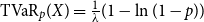 $\mathrm{TVaR}_p(X)= \frac {1}{\lambda } (1-\ln (1-p))$
, while for a lognormal distribution
$\mathrm{TVaR}_p(X)= \frac {1}{\lambda } (1-\ln (1-p))$
, while for a lognormal distribution
 $X \sim \mathrm{LN}(\mu ,\sigma ^2)$
, we have
$X \sim \mathrm{LN}(\mu ,\sigma ^2)$
, we have
 $\mathrm{TVaR}_p(X)= \frac {1}{1-p}e^{\mu +0.5\sigma ^2} \Phi \left ( \sigma - \Phi^{-1} (p) \right )$
, where
$\mathrm{TVaR}_p(X)= \frac {1}{1-p}e^{\mu +0.5\sigma ^2} \Phi \left ( \sigma - \Phi^{-1} (p) \right )$
, where
 $\Phi (\cdot )$
is the CDF of the standard normal distribution
$\Phi (\cdot )$
is the CDF of the standard normal distribution
 $\mathrm{N}(0,1)$
.
$\mathrm{N}(0,1)$
.
3.2 Premium principles
Building upon the extensive literature on optimal insurance structures, the optimal design for the Disaster Fund’s insurance coverage depends on the pricing methodology of the insurance contract. Consider a simplified scenario in which the VaR and TVaR constraints are not binding, and the upfront cost of CC is negligibleFootnote 9, then Propositions3 and 4 outline the implications of various insurance structures on the Disaster Fund.
Proposition 3.
Under the expected loss premium principle (i.e., when
 $\rho _2=0$
), the layer CC-I structure is the optimal insurance structure.
$\rho _2=0$
), the layer CC-I structure is the optimal insurance structure.
Proposition 4.
Under the standard deviation premium principle (i.e., when
 $\rho _2\gt 0$
), for sufficiently large losses (specifically for
$\rho _2\gt 0$
), for sufficiently large losses (specifically for
 $x \gt \arg _x{\{Y_I(x) = \mathrm{E}(Y_I(X))\}}$
), if the pdf of the loss distribution
$x \gt \arg _x{\{Y_I(x) = \mathrm{E}(Y_I(X))\}}$
), if the pdf of the loss distribution
 $f_X(x)$
is decreasing in
$f_X(x)$
is decreasing in
 $x$
, CC-I structure is not the optimal insurance structure.
$x$
, CC-I structure is not the optimal insurance structure.
Proposition3 indicates that when the insurance premium principle does not account for the volatility of the payout, it is always preferable to adopt the layered CC-I structure for the Disaster Fund. This is because higher-severity losses lead to a greater reduction in utility for the risk-averse government compared to lower-severity losses. In contrast, Proposition4 suggests that when the premium includes a loading based on the standard deviation of the payout, the proportional structure may be more advantageous than the CC-I structure.
In practice, due to the substantial uncertainty in characterizing disaster losses and the potentially catastrophic magnitudes of the associated payouts, insurers typically impose significant loadings on the variability of disaster risk payouts. Consequently, when
 $\rho _2$
is significant, we may observe the proportional structure outperforming the CC-I structure.
$\rho _2$
is significant, we may observe the proportional structure outperforming the CC-I structure.
3.3 Comparative statics
In this section, we perform a comparative static analysis to assess the impact of key external factors on the optimal solution, assuming that all constraints are non-binding, in order to focus on the direction of influence. To facilitate this analysis, we first introduce Lemma1.
Lemma 1.
Suppose
 $\theta ^*$
is the maximizer and
$\theta ^*$
is the maximizer and
 $\varphi \in \theta$
is one of the decision variables to optimize in Equation
13
. Moreover, assume that
$\varphi \in \theta$
is one of the decision variables to optimize in Equation
13
. Moreover, assume that
 $\frac {\partial ^2 \mathrm{E} \mathbb{U} (\theta ^*)}{\partial \varphi ^2} |_{\varphi = \varphi ^*} \lt 0$
. Then, for any exogenous variable
$\frac {\partial ^2 \mathrm{E} \mathbb{U} (\theta ^*)}{\partial \varphi ^2} |_{\varphi = \varphi ^*} \lt 0$
. Then, for any exogenous variable
 $\zeta$
(e.g.
$\zeta$
(e.g.
 $\rho _1,\rho _2, r_{CC}, F_{CC}$
or
$\rho _1,\rho _2, r_{CC}, F_{CC}$
or
 $r_e$
), if an increase (resp. decrease) in
$r_e$
), if an increase (resp. decrease) in
 $\zeta$
leads to an increase (resp. decrease) in first-order derivative
$\zeta$
leads to an increase (resp. decrease) in first-order derivative
 $\frac {\partial \mathrm{E}\mathbb{U} (\theta ^*)}{\partial \varphi }$
, the optimal
$\frac {\partial \mathrm{E}\mathbb{U} (\theta ^*)}{\partial \varphi }$
, the optimal
 $\varphi ^*$
will be increasing (resp. decreasing) in
$\varphi ^*$
will be increasing (resp. decreasing) in
 $\zeta$
.
$\zeta$
.
Lemma1 provides insights into how changes in
 $\zeta$
affect the optimal solution
$\zeta$
affect the optimal solution
 $\varphi ^*$
. It is sufficient to examine the change in
$\varphi ^*$
. It is sufficient to examine the change in
 $ \frac {\partial \mathrm{E}\mathbb{U}}{\partial \varphi }$
as
$ \frac {\partial \mathrm{E}\mathbb{U}}{\partial \varphi }$
as
 $\zeta$
varies to deduce the impact of
$\zeta$
varies to deduce the impact of
 $\zeta$
on
$\zeta$
on
 $\varphi ^*$
. Table 1 presents the comparative statics for the optimal parameters under both the proportional and CC-I structuresFootnote 10.
$\varphi ^*$
. Table 1 presents the comparative statics for the optimal parameters under both the proportional and CC-I structuresFootnote 10.
Comparative statics for the optimal parameters
 $\varphi \in \theta ^*$
under the proportional and CC-I structures in response to changes in exogenous variable
$\varphi \in \theta ^*$
under the proportional and CC-I structures in response to changes in exogenous variable
 $\xi$
. As
$\xi$
. As
 $\xi$
increases, the optimal parameter
$\xi$
increases, the optimal parameter
 $\varphi$
will either increase
$\varphi$
will either increase
 $\uparrow$
, decrease
$\uparrow$
, decrease
 $\downarrow$
, or the direction of influence is indeterminate
$\downarrow$
, or the direction of influence is indeterminate
 $\uparrow \downarrow$
. Since without imposing constraints on
$\uparrow \downarrow$
. Since without imposing constraints on
 $L$
,
$L$
,
 $L^*_{\text{CC-I}} = M^*_{\text{CC-I}}$
under the layer CC-I structure, the column for
$L^*_{\text{CC-I}} = M^*_{\text{CC-I}}$
under the layer CC-I structure, the column for
 $L^*_{\text{CC-I}}$
is excluded
$L^*_{\text{CC-I}}$
is excluded

As insurance premium becomes more expensive (i.e., higher
 $\rho _1, \rho _2$
), the government tends to adopt less insurance, reflected in higher values of
$\rho _1, \rho _2$
), the government tends to adopt less insurance, reflected in higher values of
 $L^*_{\text{prop}}$
and
$L^*_{\text{prop}}$
and
 $M^*_{\text{CC-I}}$
and lower values of
$M^*_{\text{CC-I}}$
and lower values of
 $\alpha ^*_{\text{prop}}$
,
$\alpha ^*_{\text{prop}}$
,
 $U^*_{\text{prop}}$
and
$U^*_{\text{prop}}$
and
 $U^*_{\text{CC-I}}$
. Moreover, when the upfront fee
$U^*_{\text{CC-I}}$
. Moreover, when the upfront fee
 $F_{CC}$
for arranging CC is high, the government will generally opt for less CC, leading to a higher
$F_{CC}$
for arranging CC is high, the government will generally opt for less CC, leading to a higher
 $L^*_{prop}$
and lower
$L^*_{prop}$
and lower
 $U^*_{\text{prop}}$
and
$U^*_{\text{prop}}$
and
 $U^*_{\text{CC-I}}$
. However, the effect of
$U^*_{\text{CC-I}}$
. However, the effect of
 $F_{CC}$
on
$F_{CC}$
on
 $\alpha ^*_{\text{prop}}$
and
$\alpha ^*_{\text{prop}}$
and
 $M^*_{\text{CC-I}}$
is inconclusive as higher
$M^*_{\text{CC-I}}$
is inconclusive as higher
 $F_{CC}$
can (i) reduce preference for CC due to higher cost, leading to a higher
$F_{CC}$
can (i) reduce preference for CC due to higher cost, leading to a higher
 $\alpha ^*_{\text{prop}}$
and lower
$\alpha ^*_{\text{prop}}$
and lower
 $M^*_{\text{CC-I}}$
, and (ii) deplete terminal wealth, prompting the government to reduce insurance purchase to lower premium payments and offset the wealth reduction caused by the higher upfront cost causing a lower
$M^*_{\text{CC-I}}$
, and (ii) deplete terminal wealth, prompting the government to reduce insurance purchase to lower premium payments and offset the wealth reduction caused by the higher upfront cost causing a lower
 $\alpha ^*_{\text{prop}}$
and higher
$\alpha ^*_{\text{prop}}$
and higher
 $M^*_{\text{CC-I}}$
.
$M^*_{\text{CC-I}}$
.
Similarly, the net impact of an increase in
 $r_{CC}$
on the optimal
$r_{CC}$
on the optimal
 $L^*_{\text{prop}}, U^*_{\text{prop}}$
and
$L^*_{\text{prop}}, U^*_{\text{prop}}$
and
 $M^*_{\text{CC-I}}$
is indeterminate since a higher interest rate on CC has two opposing effects: (i) deter the use of CC and propel the government to adopt insurance, which lowers
$M^*_{\text{CC-I}}$
is indeterminate since a higher interest rate on CC has two opposing effects: (i) deter the use of CC and propel the government to adopt insurance, which lowers
 $L^*_{\text{prop}}$
and
$L^*_{\text{prop}}$
and
 $M^*_{\text{CC-I}}$
and increases
$M^*_{\text{CC-I}}$
and increases
 $U^*_{\text{prop}}$
, and (ii) deplete terminal wealth due to higher loan repayment, causing the government to lower insurance purchase to in an effort to stabilize the terminal fund value, which in turn increases
$U^*_{\text{prop}}$
, and (ii) deplete terminal wealth due to higher loan repayment, causing the government to lower insurance purchase to in an effort to stabilize the terminal fund value, which in turn increases
 $L^*_{\text{prop}}$
and
$L^*_{\text{prop}}$
and
 $M^*_{\text{CC-I}}$
while decreasing
$M^*_{\text{CC-I}}$
while decreasing
 $U^*_{\text{prop}}$
.
$U^*_{\text{prop}}$
.
A higher ex-post borrowing interest rate
 $r_e$
has an unambiguous effect of increasing insurance uptake to avoid incurring substantial costs to secure additional funding for extremely large losses. Similarly, a higher risk aversion
$r_e$
has an unambiguous effect of increasing insurance uptake to avoid incurring substantial costs to secure additional funding for extremely large losses. Similarly, a higher risk aversion
 $\gamma$
motivates the government to rely more on insurance over CC and ex-post borrowing, driven by a preference to minimize volatility in the terminal Disaster Fund value.
$\gamma$
motivates the government to rely more on insurance over CC and ex-post borrowing, driven by a preference to minimize volatility in the terminal Disaster Fund value.
3.4 The VaR constraint
While the constraints
 $L \leq k_L$
and
$L \leq k_L$
and
 $U \leq k_U$
directly affect the optimal decision variables, the influence of the VaR constraint on these variables is more complex. To facilitate discussion, let
$U \leq k_U$
directly affect the optimal decision variables, the influence of the VaR constraint on these variables is more complex. To facilitate discussion, let
 $\varphi \in \{L,M,U \}$
denote a decision variable of interest and let
$\varphi \in \{L,M,U \}$
denote a decision variable of interest and let
 $\varphi ^*$
and
$\varphi ^*$
and
 $\varphi ^\#$
denote the optimal parameters for our optimization problem in Equation (13) obtained without and with VaR constraint (
$\varphi ^\#$
denote the optimal parameters for our optimization problem in Equation (13) obtained without and with VaR constraint (
 $\mathrm{VaR}_p(R_1) \geq k_{\mathrm{VaR}}$
), respectively.
$\mathrm{VaR}_p(R_1) \geq k_{\mathrm{VaR}}$
), respectively.
Proposition 5.
Under a binding VaR constraint,
 $\varphi ^\#$
will be either higher (resp. lower) than
$\varphi ^\#$
will be either higher (resp. lower) than
 $\varphi ^*$
depending on whether
$\varphi ^*$
depending on whether
 $F^{-1}_X(p_{\mathrm{VaR}})$
is higher (resp. lower) than
$F^{-1}_X(p_{\mathrm{VaR}})$
is higher (resp. lower) than
 $\varphi ^*$
.
$\varphi ^*$
.
-
• For Proportional Structure:
$F^{-1}_X(p_{\mathrm{VaR}})\lt L^* \Rightarrow L^\#\gt L^*$
, and
$F^{-1}_X(p_{\mathrm{VaR}})\gt L^* \Rightarrow L^\#\lt L^*$
.
$F^{-1}_X(p_{\mathrm{VaR}})\lt U^* \Rightarrow U^\#\lt U^*$
, and
$F^{-1}_X(p_{\mathrm{VaR}})\gt U^* \Rightarrow U^\#\gt U^*$
. -
• For CC-I Structure:
$F^{-1}_X(p_{\mathrm{VaR}})\lt M^* \Rightarrow M^\#\gt M^*$
, and
$F^{-1}_X(p_{\mathrm{VaR}})\gt M^* \Rightarrow M^\#\lt M^*$
.
$F^{-1}_X(p_{\mathrm{VaR}})\lt U^* \Rightarrow U^\#\lt U^*$
, and
$F^{-1}_X(p_{\mathrm{VaR}})\gt U^* \Rightarrow U^\#\gt U^*$
.


Proposition5 outlines the ramifications of enforcing a binding VaR constraint. Intuitively, if the VaR constraint is active and
 $p_{\mathrm{VaR}}$
-th quantile loss
$p_{\mathrm{VaR}}$
-th quantile loss
 $F^{-1}_X(p_{\mathrm{VaR}})$
is high (resp. low), the optimal strategy involves increasing (resp. decreasing) insurance coverage by reducing (resp. raising)
$F^{-1}_X(p_{\mathrm{VaR}})$
is high (resp. low), the optimal strategy involves increasing (resp. decreasing) insurance coverage by reducing (resp. raising)
 $L$
and raising (resp. lowering)
$L$
and raising (resp. lowering)
 $U$
.
$U$
.
3.5 The case of CARA utility
The Constant Absolute Risk Aversion (CARA) utility function, widely favored in the literature for its broad adoption and mathematical tractability, is expressed as
 \begin{equation*} \mathbb{U}(w;\,\gamma ) = -\mathrm{e}^{-\gamma w}, \text{ for } \gamma \gt 0. \end{equation*}
Due to the multiplicative property of exponential utility
 $\mathbb{U}(w_1 + w_2) = \mathbb{U}(w_1)\mathbb{U}(w_2)$
, the optimization problem becomes independent of the initial fund injection
$\mathbb{U}(w_1 + w_2) = \mathbb{U}(w_1)\mathbb{U}(w_2)$
, the optimization problem becomes independent of the initial fund injection
 $R_0$
when there are no VaR or TVaR constraints. In other words, the magnitude of
$R_0$
when there are no VaR or TVaR constraints. In other words, the magnitude of
 $R_0$
does not affect the values of the optimal decision variables
$R_0$
does not affect the values of the optimal decision variables
 $\theta ^*$
, and it can be omitted when VaR or TVaR constraints are absent.
$\theta ^*$
, and it can be omitted when VaR or TVaR constraints are absent.
Alternatively, if a government’s preference is governed by a CARA utility function, it is possible to endogenize the initial fund injection
 $R_0$
and determine the minimum value of
$R_0$
and determine the minimum value of
 $R_0$
necessary to satisfy the government’s risk requirement, as quantified by a VaR constraint with
$R_0$
necessary to satisfy the government’s risk requirement, as quantified by a VaR constraint with
 $p_{\mathrm{VaR}}$
above the exhaustion point
$p_{\mathrm{VaR}}$
above the exhaustion point
 $U$
. The government can first solve the expected utility maximization problem without the VaR constraint to obtain the optimal decision variables
$U$
. The government can first solve the expected utility maximization problem without the VaR constraint to obtain the optimal decision variables
 $\theta ^*$
. Subsequently, the minimum
$\theta ^*$
. Subsequently, the minimum
 $R_0$
required to satisfy the VaR requirement is
$R_0$
required to satisfy the VaR requirement is
 \begin{align} R_0 & = \inf \Big \{ r_0 \gt 0 \ | \ \mathrm{VaR}_{p_{\mathrm{VaR}}}(R_1(X);\,\theta ^*, r_0) \geq k_{\mathrm{VaR}} \Big \} \nonumber \\ & = \inf \left \{ r_0 \gt 0 \ \Bigg | \ \begin{array}{l} r_0 - C_I - C_{CC} - F^{-1}_{X}(p_{\mathrm{VaR}}) +Y_I\left (F^{-1}_{X}(p_{\mathrm{VaR}})\right ) \\ -r_{CC} Y_{CC}\left (F^{-1}_{X}(p_{\mathrm{VaR}}) \right ) -r_e Y_e\left (F^{-1}_{X}(p_{\mathrm{VaR}})\right ) \end{array} \geq k_{\mathrm{VaR}} \right \} \nonumber \\ & = k_{\mathrm{VaR}} + C_I + C_{CC} + F^{-1}_{X}(p_{\mathrm{VaR}}) - Y_I\left (F^{-1}_{X}(p_{\mathrm{VaR}})\right ) \nonumber \\ & \quad + r_{CC} Y_{CC}\left (F^{-1}_{X}(p_{\mathrm{VaR}})\right ) + r_e Y_e\left (F^{-1}_{X}(p_{\mathrm{VaR}})\right ). \end{align}
Intuitively,
 $R_0$
represents the minimum initial fund injection required to satisfy the VaR constraint
$R_0$
represents the minimum initial fund injection required to satisfy the VaR constraint
 $\mathrm{VaR}_{p_{\mathrm{VaR}}}(R_1) \geq k_{\mathrm{VaR}}$
. Graphically, as illustrated in Fig. 2, adjusting
$\mathrm{VaR}_{p_{\mathrm{VaR}}}(R_1) \geq k_{\mathrm{VaR}}$
. Graphically, as illustrated in Fig. 2, adjusting
 $R_0$
shifts the entire graph vertically upwards or downwards, while leaving the structure of the different layers (such as the reserve fund, insurance, CC, and ex-post financing) unchanged. In this context,
$R_0$
shifts the entire graph vertically upwards or downwards, while leaving the structure of the different layers (such as the reserve fund, insurance, CC, and ex-post financing) unchanged. In this context,
 $R_0$
functions as a vertical adjustment that alters the terminal fund value but does not impact the optimization procedure. The government can first determine the optimal Disaster Fund structure independently of
$R_0$
functions as a vertical adjustment that alters the terminal fund value but does not impact the optimization procedure. The government can first determine the optimal Disaster Fund structure independently of
 $R_0$
and calculate the necessary
$R_0$
and calculate the necessary
 $R_0$
to inject to meet the required VaR level
$R_0$
to inject to meet the required VaR level
 $k_{\mathrm{VaR}}$
.
$k_{\mathrm{VaR}}$
.
4. An application to the NFIP
The National Flood Insurance Program (NFIP) is a public-private partnership with a network of insurers and the federal government that provides affordable flood insurance protection for households and commercial buildings in the United States (FEMA, 2024a). Managed by the Federal Emergency Management Agency (FEMA), the NFIP serves over five million policyholders, with more than
 $\$$
1.3 trillion in coverage (FEMA, 2024a). NFIP is one of the largest government flood insurance programs in the world (Michel-Kerjan and Kunreuther, Reference Michel-Kerjan and Kunreuther2011).
$\$$
1.3 trillion in coverage (FEMA, 2024a). NFIP is one of the largest government flood insurance programs in the world (Michel-Kerjan and Kunreuther, Reference Michel-Kerjan and Kunreuther2011).
To fund claims payments following disaster occurrences, the NFIP relies not only on premium proceeds from flood insurance policies but also on private reinsurance and catastrophe bonds. In the year 2020 alone, NFIP secured
 $\$$
1.33 billion in disaster loss coverage through agreements with 27 reinsurers, paying an aggregate premium of
$\$$
1.33 billion in disaster loss coverage through agreements with 27 reinsurers, paying an aggregate premium of
 $\$$
205 million. Additionally, in February 2020, FEMA issued
$\$$
205 million. Additionally, in February 2020, FEMA issued
 $\$$
400 million in catastrophe bonds, incurring a first-year premium cost of
$\$$
400 million in catastrophe bonds, incurring a first-year premium cost of
 $\$$
50.28 million (Horn and Webel, Reference Horn and Webel2024; FEMA, 2024b)Footnote 11. Once these funding sources are exhausted, the NFIP can access its borrowing authority to secure loans from the Treasury. By the end of 2020, the NFIP’s cumulative debt to the Treasury stood at
$\$$
50.28 million (Horn and Webel, Reference Horn and Webel2024; FEMA, 2024b)Footnote 11. Once these funding sources are exhausted, the NFIP can access its borrowing authority to secure loans from the Treasury. By the end of 2020, the NFIP’s cumulative debt to the Treasury stood at
 $\$$
20.5 billion (Horn, Reference Horn2024).
$\$$
20.5 billion (Horn, Reference Horn2024).
Structurally, our Disaster Fund model closely aligns with the NFIP’s financing mechanism. Low-severity losses are absorbed directly, medium-severity risks are shared with external parties, and extremely large losses are managed through borrowings. From a cash flow perspective, both purchasing reinsurance and issuing catastrophe bonds function similarly, as they involve regular payments in exchange for financial protection in the event of a loss. As a result, in our Disaster Fund model, these mechanisms are grouped together under insurance. To enhance the model’s versatility, especially for less developed countries, we also incorporate a CC line. Setting
 $F_{CC}=r_{CC}=0$
effectively removes CC from the model, allowing flexibility to align with varying financial structures.
$F_{CC}=r_{CC}=0$
effectively removes CC from the model, allowing flexibility to align with varying financial structures.
4.1 Data
Using the loss data from OpenFEMAFootnote 12, we employ the NFIP as a case study to explore the construction of the Disaster Fund for flood risk management under various practical constraints and considerations. To ensure relevance and avoid potential seasonality, we aggregate all individual claims and policies at the annual level and restrict the data to the period from 2002 to 2020Footnote 13. While most flood insurance policies are single-year contracts, a subset of policies spans multiple years; for these, we distribute the total premium amount evenly across all applicable years. Furthermore, to ensure the claims data possess similar exposures across years, we calculate the annual premium growth rate over the last 12 years (2009 to 2020), which is approximately 4%, and inflate the annual claims data by a factor of
 $1.04^{(2020 - Year)}$
to bring all losses to 2020 exposure levels. By scaling all claims data to 2020 levels, we account for both the growing number of policyholders and the effects of inflation. Additionally, we conduct several time-series analyses (at
$1.04^{(2020 - Year)}$
to bring all losses to 2020 exposure levels. By scaling all claims data to 2020 levels, we account for both the growing number of policyholders and the effects of inflation. Additionally, we conduct several time-series analyses (at
 $5\%$
significance level) to ensure that the loss data (i) is homoskedastic (Breusch-Pagan test), (ii) has no autocorrelation (Breusch-Godfrey and Ljung-box test), (iii) is stationary (ADF and KPSS test), and (iv) is absent of time trend (regression slope t-test). Moreover, we rescale the loss data by dividing by
$5\%$
significance level) to ensure that the loss data (i) is homoskedastic (Breusch-Pagan test), (ii) has no autocorrelation (Breusch-Godfrey and Ljung-box test), (iii) is stationary (ADF and KPSS test), and (iv) is absent of time trend (regression slope t-test). Moreover, we rescale the loss data by dividing by
 $\$$
10 billion for brevity. Next, we fit the loss data to several candidate distributions – including Weibull, gamma, and lognormal – using the maximum likelihood estimation method. Among all distributions, the lognormal distribution emerges as the best fit, as it achieves the lowest Kolmogorov-Smirnov, Cramer-von Mises, and Anderson-Darling test statistics, as well as the lowest AIC and BIC values. The fitted loss distribution is
$\$$
10 billion for brevity. Next, we fit the loss data to several candidate distributions – including Weibull, gamma, and lognormal – using the maximum likelihood estimation method. Among all distributions, the lognormal distribution emerges as the best fit, as it achieves the lowest Kolmogorov-Smirnov, Cramer-von Mises, and Anderson-Darling test statistics, as well as the lowest AIC and BIC values. The fitted loss distribution is
 $X \sim LN(\mu = -1.466,\sigma ^2 = 1.096^2)$
.
$X \sim LN(\mu = -1.466,\sigma ^2 = 1.096^2)$
.
We set
 $k_U$
at the 99.8th percentile of the loss distribution, corresponding to the highest recurrence interval of a 1-in-500-year event, as documented by FEMA (e.g., FEMA, 2021). Additionally, we set
$k_U$
at the 99.8th percentile of the loss distribution, corresponding to the highest recurrence interval of a 1-in-500-year event, as documented by FEMA (e.g., FEMA, 2021). Additionally, we set
 $k_L$
to align with the common rule of thumb in literature and practice, where 1-in-10-year period losses are retained. Both
$k_L$
to align with the common rule of thumb in literature and practice, where 1-in-10-year period losses are retained. Both
 $p_{\mathrm{VaR}}$
and
$p_{\mathrm{VaR}}$
and
 $p_{\mathrm{TVaR}}$
are set at 99.8% to be consistent with
$p_{\mathrm{TVaR}}$
are set at 99.8% to be consistent with
 $U$
, following Proposition1. Without the loss of generality, we focus on the VaR constraint and set
$U$
, following Proposition1. Without the loss of generality, we focus on the VaR constraint and set
 $k_{\mathrm{VaR}} = 26$
for illustrative purposes to effectively demonstrate the functionality of the Disaster Fund modelFootnote 14.
$k_{\mathrm{VaR}} = 26$
for illustrative purposes to effectively demonstrate the functionality of the Disaster Fund modelFootnote 14.
For the simulation exercise, we adopt the CARA utility with an initial fund injection of
 $R_0 = 29.181$
, which corresponds to the 99.9995th percentile of the loss distribution. Under expected utility theory, it is widely known that wealth and risk aversion are indistinguishable (Yaari, Reference Yaari1987). We will put less emphasis on
$R_0 = 29.181$
, which corresponds to the 99.9995th percentile of the loss distribution. Under expected utility theory, it is widely known that wealth and risk aversion are indistinguishable (Yaari, Reference Yaari1987). We will put less emphasis on
 $R_0$
and focus on highlighting the characteristics of the DRF model. Moreover, as established in Section 3.5, when a CARA utility function is adopted and the VaR constraint is non-binding,
$R_0$
and focus on highlighting the characteristics of the DRF model. Moreover, as established in Section 3.5, when a CARA utility function is adopted and the VaR constraint is non-binding,
 $R_0$
does not influence the optimal decision parameters. Next, we set the necessary input parameters, referring to Clarke
et al. Reference Clarke, Mahul, Poulter and Teh(2017) for guidance. In practice, governments tailor these parameters to reflect their specific requirements, economic conditions, and risk profiles. A summary of all parameter values can be found in Table 2.
$R_0$
does not influence the optimal decision parameters. Next, we set the necessary input parameters, referring to Clarke
et al. Reference Clarke, Mahul, Poulter and Teh(2017) for guidance. In practice, governments tailor these parameters to reflect their specific requirements, economic conditions, and risk profiles. A summary of all parameter values can be found in Table 2.
Parameters for the Disaster Fund model for empirical simulations

4.2 Empirical findings
(a) and (b) show the optimal parameters
 $\theta ^*$
; (c) shows the differences in expected utility between the insurance structures; (d) and (e) show the amount of insurance and contingent credit; and (f) shows the
$\theta ^*$
; (c) shows the differences in expected utility between the insurance structures; (d) and (e) show the amount of insurance and contingent credit; and (f) shows the
 $VaR_{99.5\%}$
value for both insurance structures. All plots depict risk aversion parameter
$VaR_{99.5\%}$
value for both insurance structures. All plots depict risk aversion parameter
 $\gamma \in [0,10]$
and premium loading
$\gamma \in [0,10]$
and premium loading
 $\rho _2 \in [0,1]$
. Optimization adopts CARA utility and parameters from Table 2. To make
$\rho _2 \in [0,1]$
. Optimization adopts CARA utility and parameters from Table 2. To make
 $\alpha ^*$
span the entire vertical axis for illustrative purposes, we multiply
$\alpha ^*$
span the entire vertical axis for illustrative purposes, we multiply
 $k_U=5.4$
(upper limit of the plot) to
$k_U=5.4$
(upper limit of the plot) to
 $\alpha ^* \in [0,1]$
so that its new range becomes
$\alpha ^* \in [0,1]$
so that its new range becomes
 $[0,5.4]$
.
$[0,5.4]$
.

4.2.1 Base case
Fig. 3 presents the optimal decision variables, including the optimal amounts of insurance and CC for mid-severity losses, as well as the comparison between the expected utility and the VaR of the terminal Disaster Fund value, as derived from the maximization problem in Equation 13. From Figs. 3(a) and (b), two distinct extremes in
 $\theta ^* \in \Theta$
can be observed. When risk aversion
$\theta ^* \in \Theta$
can be observed. When risk aversion
 $\gamma$
is high and premium loading
$\gamma$
is high and premium loading
 $\rho _2$
is low, the mid-severity loss layer is predominantly covered by insurance, with minimal to no reliance on CC. As
$\rho _2$
is low, the mid-severity loss layer is predominantly covered by insurance, with minimal to no reliance on CC. As
 $\gamma$
decreases and
$\gamma$
decreases and
 $\rho _2$
increases, the amount of insurance reduces while CC usage rises. In contrast, at the opposite extreme, where
$\rho _2$
increases, the amount of insurance reduces while CC usage rises. In contrast, at the opposite extreme, where
 $\gamma$
is low and
$\gamma$
is low and
 $\rho _2$
is high, the VaR constraint becomes binding, resulting in a minimal amount of insurance required to meet the VaR requirement, as indicated by the plateauing of
$\rho _2$
is high, the VaR constraint becomes binding, resulting in a minimal amount of insurance required to meet the VaR requirement, as indicated by the plateauing of
 $\alpha ^*$
and
$\alpha ^*$
and
 $M^*$
. This aligns with our intuition, where higher risk aversion and lower insurance premium loading incentivize the government to shift from CC to insurance. When less insurance is purchased, the VaR constraint is more likely to be violated.
$M^*$
. This aligns with our intuition, where higher risk aversion and lower insurance premium loading incentivize the government to shift from CC to insurance. When less insurance is purchased, the VaR constraint is more likely to be violated.
In practice, it is crucial for the government to identify which region it falls into. If the government has high risk aversion and its VaR constraint is not binding, it will face significant price risk for disaster insurance, as its demand for insurance is highly price inelastic. In this case, the government is vulnerable to fluctuations or inflation in the insurance market. Conversely, if the government operates under an active VaR constraint, the optimal amount of insurance becomes extremely sensitive to the government’s chosen threshold
 $k_{\mathrm{Var}}$
, and insurance decisions are no longer driven solely by utility maximization. By relaxing the VaR constraint (i.e., decreasing
$k_{\mathrm{Var}}$
, and insurance decisions are no longer driven solely by utility maximization. By relaxing the VaR constraint (i.e., decreasing
 $k_{\mathrm{Var}}$
), the government can significantly influence its insurance amount and move closer to the optimal utility-maximizing level of insurance. Lastly, if the government falls into the middle region, where the VaR constraint is not binding and the optimal amount of insurance and CC changes rapidly across
$k_{\mathrm{Var}}$
), the government can significantly influence its insurance amount and move closer to the optimal utility-maximizing level of insurance. Lastly, if the government falls into the middle region, where the VaR constraint is not binding and the optimal amount of insurance and CC changes rapidly across
 $\gamma$
and
$\gamma$
and
 $\rho _2$
, the optimal fund construction is highly sensitive to the model’s parameters and assumptions, such as the shape of the utility function and the magnitude of the risk aversion parameter. These factors are often difficult to measure accurately and are prone to miscalibration in practice. Greater care should be taken when interpreting the outputs of the Disaster Fund model in this context.
$\rho _2$
, the optimal fund construction is highly sensitive to the model’s parameters and assumptions, such as the shape of the utility function and the magnitude of the risk aversion parameter. These factors are often difficult to measure accurately and are prone to miscalibration in practice. Greater care should be taken when interpreting the outputs of the Disaster Fund model in this context.
4.2.2 Proportional structure vs CC-I structure
From Fig. 3(d) and (e), both the proportional and layer CC-I structures generally suggest comparable amounts of insurance and CC. Consequently, both structures exhibit similar VaR values, as shown in Fig. 3(f). However, Fig. 3(c) indicates that the layer CC-I structure outperforms the proportional structure since it yields a higher expected utility
 $\mathrm{E}\mathbb{U}_{\text{CC-I}} \geq \mathrm{E} \mathbb{U}_{\text{prop}}$
, particularly for low
$\mathrm{E}\mathbb{U}_{\text{CC-I}} \geq \mathrm{E} \mathbb{U}_{\text{prop}}$
, particularly for low
 $\gamma$
and high
$\gamma$
and high
 $\rho _2$
. The flexibility of the CC-I structure, particularly the lack of a common attachment point
$\rho _2$
. The flexibility of the CC-I structure, particularly the lack of a common attachment point
 $L$
for insurance and CC, enables the government to purchase insurance only for high-severity losses. This flexibility makes the CC-I structure superior to the proportional structure in utility maximization.
$L$
for insurance and CC, enables the government to purchase insurance only for high-severity losses. This flexibility makes the CC-I structure superior to the proportional structure in utility maximization.
One puzzling question remains: under what circumstances will the proportional structure outperform the CC-I structure? To explore this, we simulate the optimal parameters without constraining the exhaustion point
 $U$
, effectively letting
$U$
, effectively letting
 $k_U \rightarrow \infty$
. We plot the results in Fig. B.7 in Appendix B and find that the proportional structure will dominate the CC-I structure only at extremely high loss quantiles. To ensure robustness, we repeat the experiment using a Gamma loss distribution, which is less skewed and has a smaller tail compared to the lognormal distribution, leading to lower quantile values. Similarly, we observe that the proportional structure can still outperform the layer CC-I structure. The optimal
$k_U \rightarrow \infty$
. We plot the results in Fig. B.7 in Appendix B and find that the proportional structure will dominate the CC-I structure only at extremely high loss quantiles. To ensure robustness, we repeat the experiment using a Gamma loss distribution, which is less skewed and has a smaller tail compared to the lognormal distribution, leading to lower quantile values. Similarly, we observe that the proportional structure can still outperform the layer CC-I structure. The optimal
 $U^*$
is approximately
$U^*$
is approximately
 $9.3$
, which corresponds to a
$9.3$
, which corresponds to a
 $106,903$
-year return period.
$106,903$
-year return period.
When considering losses of exceedingly high magnitudes, the proportional structure may outperform the layer CC-I structure, as it allows for partial coverage of each marginal unit of loss. This reduces the overall variability of the insurance payoff and can lead to substantial premium reductions, particularly when the premium loading
 $\rho _2$
is large and the loss severity is high. However, it remains uncertain whether such extreme loss quantiles are realistic or fall within the risk horizon of any government or Disaster Fund’s objectives.
$\rho _2$
is large and the loss severity is high. However, it remains uncertain whether such extreme loss quantiles are realistic or fall within the risk horizon of any government or Disaster Fund’s objectives.
4.2.3 Influence of higher-order moments
Disaster losses are often characterized by significant right skewness and fat tails, reflecting the frequent occurrence of extreme events. While the impact of the mean and variance of the loss distribution on optimal insurance decisions is well-established and intuitive, the influence of higher-order moments, such as skewness and kurtosis, is less direct and has not been as extensively studied. In this section, we investigate how the higher moments of the disaster loss distribution affect the optimal construction of the Disaster Fund.
Under fat-tailed losses, the government tends to purchase more insurance. When comparing Figs. 4(a)–(d) with Figs. 3(a)–(b), we observe that higher-order moments cause the region where insurance and CC change rapidly (referred to as the middle region in Section 4.2.1) to shift toward higher values of
 $\gamma$
and lower values of
$\gamma$
and lower values of
 $\rho _2$
. This trend is also apparent in Figs. 4(e)–(f), where the amount of insurance is lowest under
$\rho _2$
. This trend is also apparent in Figs. 4(e)–(f), where the amount of insurance is lowest under
 $X_3$
, followed by
$X_3$
, followed by
 $X_2$
, and then
$X_2$
, and then
 $X_1$
for any given (
$X_1$
for any given (
 $\gamma , \rho _2$
)-pair.
$\gamma , \rho _2$
)-pair.
Moreover, the region where insurance and CC change rapidly is narrowest under the lognormal distribution, indicating that, under highly skewed and fat-tailed losses, the government is more likely to lien toward either one extreme – (I) arrange for insurance without any CC or (2) purchase the minimum amount of insurance necessary to meet the VaR constraint – and less probable to adopt a mix of insurance and CC above the VaR requirement.
Three illustrative loss distributions, along with their first four moments.
 $X_1$
corresponds to the best-fit loss distribution in Section 4.1.
$X_1$
corresponds to the best-fit loss distribution in Section 4.1.
 $X_2$
and
$X_2$
and
 $X_3$
are two alternative distributions fitted with the same first two moments but possess smaller higher-order moments
$X_3$
are two alternative distributions fitted with the same first two moments but possess smaller higher-order moments


4.2.4 Utility function
For robustness, we repeated the analysis using the Constant Relative Risk Aversion (CRRA) utility function, with the results presented in Fig. B.8 in Appendix B. The key characteristics of the Disaster Fund remain consistent with those observed under the CARA utility function. This simulation refutes concerns that the DRF model is highly sensitive to small variations in risk aversion or overly dependent on the specific form of the utility function.
4.3 Optimal parameters under the Disaster Fund model
Optimal decision variables across risk aversion parameter
 $\gamma$
under the (a) proportional and (b) layer CC-I structure, with
$\gamma$
under the (a) proportional and (b) layer CC-I structure, with
 $\rho _2 = 0.2$
and all remaining parameter values from Table 2. The top red line denotes
$\rho _2 = 0.2$
and all remaining parameter values from Table 2. The top red line denotes
 $U^*$
, and the bottom green line denotes
$U^*$
, and the bottom green line denotes
 $L^*$
. The middle gray line represents
$L^*$
. The middle gray line represents
 $\alpha ^*$
for the (a) proportional structure and
$\alpha ^*$
for the (a) proportional structure and
 $M^*$
for the (b) CC-I structure. The red area denotes the proportion (for proportional structure) or amount (for CC-I structure) of insurance, while the green area represents the proportion/amount of contingent credit. The dashed line highlights
$M^*$
for the (b) CC-I structure. The red area denotes the proportion (for proportional structure) or amount (for CC-I structure) of insurance, while the green area represents the proportion/amount of contingent credit. The dashed line highlights
 $\gamma = 0.2$
, which is used in the discussion.
$\gamma = 0.2$
, which is used in the discussion.

Finally, we apply our Disaster Fund model to the NFIP to analyze its optimal combination of disaster financing tools. For illustration, in addition to the parameters in Table 2, we assume that insurance is available to NFIP at
 $\rho _2 = 0.2$
, and that NFIP’s preferences are represented by a CARA utility function with a risk aversion parameter of 0.2.
$\rho _2 = 0.2$
, and that NFIP’s preferences are represented by a CARA utility function with a risk aversion parameter of 0.2.
From Fig. 5(a), under the proportional strategy, the government should arrange insurance and CC to cover losses between
 $\$$
9 billion and
$\$$
9 billion and
 $\$$
47 billion, with insurance covering 65% of the losses. The expected terminal value of the Disaster Fund in this case is
$\$$
47 billion, with insurance covering 65% of the losses. The expected terminal value of the Disaster Fund in this case is
 $\$$
287 billion, with a standard deviation of
$\$$
287 billion, with a standard deviation of
 $\$$
2.01 billion.
$\$$
2.01 billion.
Similarly, Fig. 5(b) shows that under the CC-I strategy, the optimal configuration is to arrange CC for losses from
 $\$$
9 billion (
$\$$
9 billion (
 $L=0.9$
) to
$L=0.9$
) to
 $\$$
22 billion (
$\$$
22 billion (
 $M=2.2$
) and purchase insurance for losses between
$M=2.2$
) and purchase insurance for losses between
 $\$$
22 billion and
$\$$
22 billion and
 $\$$
46 billion (
$\$$
46 billion (
 $U^*=4.6$
). This corresponds to
$U^*=4.6$
). This corresponds to
 $\$$
13 billion of CC and
$\$$
13 billion of CC and
 $\$$
24 billion of insurance coverage. The expected terminal value of the Disaster Fund remains
$\$$
24 billion of insurance coverage. The expected terminal value of the Disaster Fund remains
 $\$$
287 billion, while the standard deviation increases to
$\$$
287 billion, while the standard deviation increases to
 $\$$
2.82 billion.
$\$$
2.82 billion.
For the VaR constraint to become binding, the threshold
 $k_{\mathrm{VaR}}$
must be set above
$k_{\mathrm{VaR}}$
must be set above
 $\$$
244.5 billion.
$\$$
244.5 billion.
4.4 An alternative budget constraint
As robustness check, we consider the budget constraint
 $L + C_{\text{I}} + C_{\text{CC}}$
as an alternative specification to our limited reserve constraint
$L + C_{\text{I}} + C_{\text{CC}}$
as an alternative specification to our limited reserve constraint
 $L \leq k_L$
. This budget constraint caps the total initial monetary outlay prior to loan repayments at
$L \leq k_L$
. This budget constraint caps the total initial monetary outlay prior to loan repayments at
 $k_L$
, thereby imposing an upper limit on the total insurance premium and the upfront cost of arranging CC, with all remaining funds allocated to the costless reserve fund.
$k_L$
, thereby imposing an upper limit on the total insurance premium and the upfront cost of arranging CC, with all remaining funds allocated to the costless reserve fund.
Base case results replicating Fig. 3 with the alternative constraint
 $L+C_I+C_{CC} \leq k_L$
.
$L+C_I+C_{CC} \leq k_L$
.

Fig. 6 replicates Fig. 3 after replacing the limited reserve constraint
 $L \leq k_L$
with the budget constraint
$L \leq k_L$
with the budget constraint
 $L + C_I + C_{CC} \leq k_L$
. Our empirical findings remain largely consistent under the budget constraint framework, as evidenced by the close resemblance between Figs. 3 and 6. The key distinction introduced by the budget constraint specification is the minor reallocation of funds, characterized as a small transfer from CC adoption to the costless reserve fund. However, the magnitude of these changes is relatively insignificant.
$L + C_I + C_{CC} \leq k_L$
. Our empirical findings remain largely consistent under the budget constraint framework, as evidenced by the close resemblance between Figs. 3 and 6. The key distinction introduced by the budget constraint specification is the minor reallocation of funds, characterized as a small transfer from CC adoption to the costless reserve fund. However, the magnitude of these changes is relatively insignificant.
For the layer CC-I strategy, in the absence of the VaR constraint, the optimal
 $M^*$
and
$M^*$
and
 $U^*$
are identical to those obtained under the limited reserve constraint, indicating that the amount of insurance and the severity of insured losses remain unchanged. For low levels of risk aversion
$U^*$
are identical to those obtained under the limited reserve constraint, indicating that the amount of insurance and the severity of insured losses remain unchanged. For low levels of risk aversion
 $\gamma$
and the standard deviation loading factor
$\gamma$
and the standard deviation loading factor
 $\rho _2$
, the optimal
$\rho _2$
, the optimal
 $L^*$
also remains across both constraints. However, for higher values of
$L^*$
also remains across both constraints. However, for higher values of
 $\gamma$
and
$\gamma$
and
 $\rho _2$
, the budget constraint slightly increases the optimal
$\rho _2$
, the budget constraint slightly increases the optimal
 $L^*$
, as it induces a substitution effect from CC toward the reserve fund. Given that the reserve fund does not incur an upfront cost, the government prioritizes its full utilization before resorting to CC. Nonetheless, since the upfront cost of CC
$L^*$
, as it induces a substitution effect from CC toward the reserve fund. Given that the reserve fund does not incur an upfront cost, the government prioritizes its full utilization before resorting to CC. Nonetheless, since the upfront cost of CC
 $F_{text{CC}}$
is relatively small, the overall impact is minimal.
$F_{text{CC}}$
is relatively small, the overall impact is minimal.
On the other hand, when the VaR constraint is binding,
 $L^*$
becomes marginally higher compared to the non-binding VaR constraint case, particularly for low
$L^*$
becomes marginally higher compared to the non-binding VaR constraint case, particularly for low
 $\gamma$
and
$\gamma$
and
 $\rho _2$
values. Since the amount of insurance is fixed at a minimum level to satisfy the VaR requirement, the new budget constraint allows slightly more CC to be substituted with reserve fund. Moreover, as the total budget
$\rho _2$
values. Since the amount of insurance is fixed at a minimum level to satisfy the VaR requirement, the new budget constraint allows slightly more CC to be substituted with reserve fund. Moreover, as the total budget
 $k_L$
increases under the new constraint, the allocation to the reserve fund
$k_L$
increases under the new constraint, the allocation to the reserve fund
 $L^*$
rises, especially when
$L^*$
rises, especially when
 $\gamma$
is low and
$\gamma$
is low and
 $\rho _2$
is high. In contrast, the value of
$\rho _2$
is high. In contrast, the value of
 $M^*$
exhibits only a marginal increase and exhaustion point of
$M^*$
exhibits only a marginal increase and exhaustion point of
 $U^*$
remains relatively constant.Footnote 15 Intuitively, the increase in
$U^*$
remains relatively constant.Footnote 15 Intuitively, the increase in
 $k_L$
induces only a minor reallocation from CC to the costless reserve fund, with negligible impact on the overall balance between risk transfer (insurance) and risk retention (CC and reserve fund) mechanisms.
$k_L$
induces only a minor reallocation from CC to the costless reserve fund, with negligible impact on the overall balance between risk transfer (insurance) and risk retention (CC and reserve fund) mechanisms.
A similar pattern emerges under the proportional strategy. Under the new budget constraint, both the optimal
 $L^*$
and
$L^*$
and
 $\alpha ^*$
increase, while optimal
$\alpha ^*$
increase, while optimal
 $U^*$
remains relatively stable. Consistent with the observations under the layer CC-I strategy, the model favors greater reliance on the reserve fund at the expense of CC, with insurance coverage remaining essentially unchanged relative to the limited reserve constraint. Additionally, there is a modest shift toward insuring more severe losses, with both
$U^*$
remains relatively stable. Consistent with the observations under the layer CC-I strategy, the model favors greater reliance on the reserve fund at the expense of CC, with insurance coverage remaining essentially unchanged relative to the limited reserve constraint. Additionally, there is a modest shift toward insuring more severe losses, with both
 $L^*$
and
$L^*$
and
 $\alpha ^*$
rising to preserve the same total insurance coverage. The presence of the VaR constraint leads to a more pronounced increase in
$\alpha ^*$
rising to preserve the same total insurance coverage. The presence of the VaR constraint leads to a more pronounced increase in
 $L^*$
and
$L^*$
and
 $\alpha ^*$
, while
$\alpha ^*$
, while
 $U^*$
decreases slightly to preserve the total amount of insurance coverage. As the constraint is relaxed through higher values of
$U^*$
decreases slightly to preserve the total amount of insurance coverage. As the constraint is relaxed through higher values of
 $k_L$
,
$k_L$
,
 $L^*$
increases,
$L^*$
increases,
 $U^*$
stays constant, and
$U^*$
stays constant, and
 $\alpha ^*$
increases slightly, resulting in a negligible influence on the amount of insurance uptake and a slight decline in CC arrangement.
$\alpha ^*$
increases slightly, resulting in a negligible influence on the amount of insurance uptake and a slight decline in CC arrangement.
Overall, the differences in the optimal DRF structure between the limited reserve constraint and the budget constraint are negligible.
5. Conclusion and discussion
With the increasing severity and frequency of disasters driven by climate change, it has become more critical than ever for governments to develop comprehensive DRF strategies to mitigate the severe social, political, humanitarian, and environmental consequences. While a variety of DRF instruments are available, each comes with its own strengths and limitations.Footnote 16 Therefore, it is essential to identify the optimal combination of these instruments and plan well in advance before a disaster occurs. Sound disaster preparedness is fundamental to ensuring a country’s resilience, stability, and long-term prosperity.
We propose a highly flexible and interpretable Disaster Fund model that integrates several practical aspects of DRF design. Governments often operate with limited reserves and constrained risk horizons due to budgetary limitations, short-term planning, or myopic risk assessment. Under extreme risk, governments also exhibit risk aversion – an important factor that much of the existing DRF literature overlooks for the sake of simplification. Our model further incorporates familiar insurance structures prevalent in the (re)insurance market, including excess-of-loss and proportional insurance, along with common premium loadings based on the expected value and standard deviation of insurance payouts. By leveraging a utility maximization framework, we analytically derive various comparative statics and apply our model to the NFIP dataset.
Our findings are extensive and provide significant insights into the design of DRF strategies. We establish analytically that the VaR and TVaR requirements are equivalent under a limited risk horizon, allowing regulators to focus on managing one risk requirement (typically VaR since it is simpler to understand and calculate). In addition, we demonstrate that the proportional structure can outperform the layer CC-I structure, particularly when insurers impose a high premium loading on payout variability and the government has a long risk horizon. Our empirical case study further validates this result. We perform comparative statics of several key exogenous variables, and the results largely align with our intuition. Furthermore, we analytically identify how the optimal parameters respond to the imposition of a binding VaR constraint, offering clarity on its effects. Empirically, we fit the claims and premium data from NFIP into our DRF model and identify the existence and significance of several prominent regions that characterize a government’s DRF strategy. Moreover, after accounting for the mean and variance, a highly skewed and fat-tailed loss distribution encourages higher insurance adoption and reduces the government’s likelihood of mixing insurance and CC. Lastly, we show that our results are robust under various utility functions and illustrate a possible construction of the Disaster Fund model for flood losses. These findings contribute to both the theoretical understanding and practical implementation of DRF strategies, ensuring governments are better prepared to manage catastrophic losses effectively.
While our analysis is based on a stylized model, it is important to acknowledge that, in real-world settings, additional intangible or institutional costs may exist that are not explicitly captured in our framework. For example, access to CC facilities provided by supranational institutions such as the World Bank is often conditional on the implementation of satisfactory policy frameworks and disaster risk management programs. These may include stringent repayment schedules, requirements for disaster relief plans, and constraints on capital structure, which can limit a country’s fiscal sovereignty and operational flexibility. Consequently, countries may perceive insurance, particularly parametric or index-linked contracts with fewer administrative and policy requirements, as a simpler and less restrictive alternative. Furthermore, eligibility criteria and country-specific borrowing limits may constrain access to CC facilities, leading some countries to favor insurance solutions. Limited experience in DRF and management can also influence preferences. For instance, uncertainty about the distribution of disaster-related losses or the trajectory of future interest rates may prompt policymakers to prefer insurance instruments, which offer predefined payouts and eliminate exposure to such unknown risks, unlike CC, which shifts the burden into the future and introduces repayment uncertainty. Additionally, insurance premiums may not always follow a simple expected loss or standard deviation-based pricing principle. For moderate loss events, insurance may be priced favorably due to better insurability, making the insurance-CC hybrid Insurance-Contingent Credit (I-CC) strategy economically attractive in practice.
DRF is a highly complex process. The Disaster Fund model requires that the government specify its utility function and understand the premium principles used by insurers, which should be analyzed empirically before adopting the DRF model. More advanced disaster loss modeling techniques can significantly improve the accuracy and practical relevance of the results and recommendations. Additionally, extending the model to include other unique risk requirements beyond VaR and TVaR would be straightforward and beneficial.
We believe that our proposed methodology and findings can inspire future research in this area and contribute to the limited body of quantitative DRF literature. Future research can explore the following directions: (i) derive closed-form solutions to the optimization problem, (ii) incorporate additional DRF instruments into the Disaster Fund model, (iii) expand the range of considerations and constraints, such as limited insurance capacity and maximum CC, (iv) develop a more concrete methodology for governments to determine values of exogenous variables such as
 $k_U, k_L, k_{\mathrm{VaR}}$
, and
$k_U, k_L, k_{\mathrm{VaR}}$
, and
 $k_{\mathrm{TVaR}}$
(or endogenize them into the model), and (v) extend the model to a multi-period framework.
$k_{\mathrm{TVaR}}$
(or endogenize them into the model), and (v) extend the model to a multi-period framework.
Funding statement
Tan acknowledges research funding from Nanyang Business School International PhD Scholarship. Zhang acknowledges the research funding support from the Singapore Ministry of Education Academic Research Fund Tier 1 Grant (RG49/24).
Competing interests
The authors declare that they have no conflict of interest.
Data availability statement
The authors confirm that the data and code supporting the findings of this study are available as supplementary materials accompanying the article.
A. Appendix: Proofs
A.1 Proof of Proposition 1
For every
 $p \geq p_U$
, we have
$p \geq p_U$
, we have
 $\mathrm{VaR}_{p}(R_1) = \mathrm{VaR}_{p_U}(R_1)-(1+r_e)(F^{-1}_X(p)-U)$
. Therefore,
$\mathrm{VaR}_{p}(R_1) = \mathrm{VaR}_{p_U}(R_1)-(1+r_e)(F^{-1}_X(p)-U)$
. Therefore,
 $\forall \ p_1,$
 $p_2 \geq p_U$
,
$p_2 \geq p_U$
,
 \begin{eqnarray*} \mathrm{VaR}_{p_1}(R_1) &=& \mathrm{VaR}_{p_U}(R_1)-(1+r_e)(F^{-1}_X(p_1)-U) \\ &=& \mathrm{VaR}_{p_2}(R_1) - (1+r_e)(F^{-1}_X(p_1) - F^{-1}_X(p_2)). \end{eqnarray*}
Hence,
 $\mathrm{VaR}_{p_1}(R_1) \geq k_{\mathrm{VaR}}$
if and only if
$\mathrm{VaR}_{p_1}(R_1) \geq k_{\mathrm{VaR}}$
if and only if
 $\mathrm{VaR}_{p_2}(R_1) \geq k_{\mathrm{VaR}} + (1+r_e)(F^{-1}_X(p_1) - F^{-1}_X(p_2))$
.
$\mathrm{VaR}_{p_2}(R_1) \geq k_{\mathrm{VaR}} + (1+r_e)(F^{-1}_X(p_1) - F^{-1}_X(p_2))$
.
A.2 Proof of Proposition 2
By Proposition1 we have,
 \begin{eqnarray*} \mathrm{TVaR}_{p}(R_1) &=& \frac {1}{1-p} \int ^1_p \mathrm{VaR}_q(R_1) \mathop {}\!\mathrm{d} q \\ &=& \frac {1}{1-p} \int ^1_p \left [ \mathrm{VaR}_p(R_1) - (1+r_e)(F^{-1}_X(q) - F^{-1}_X(p)) \right ] \mathop {}\!\mathrm{d} q \\ &=& \mathrm{VaR}_p(R_1) - (1+r_e) \left (\frac {1}{1-p}\int ^1_p F^{-1}_X(q) \mathop {}\!\mathrm{d} q \right ) + (1+r_e)F^{-1}_X(p) \\ &=& \mathrm{VaR}_p(R_1) - (1+r_e) \mathrm{TVaR}_p(X) + (1+r_e)F^{-1}_X(p). \end{eqnarray*}
Hence,
 $\mathrm{TVaR}_p(R_1) \geq k_{\mathrm{TVaR}}$
if and only if
$\mathrm{TVaR}_p(R_1) \geq k_{\mathrm{TVaR}}$
if and only if
 $\mathrm{VaR}_p(R_1) \geq k_{\mathrm{TVaR}} - (1+r_e) F^{-1}_X(p) + (1+r_e) \mathrm{TVaR}_p(X)$
.
$\mathrm{VaR}_p(R_1) \geq k_{\mathrm{TVaR}} - (1+r_e) F^{-1}_X(p) + (1+r_e) \mathrm{TVaR}_p(X)$
.
A.3 Proof of Proposition 3
We consider the optimization problem under the parameter space
 $\Theta$
where the constraints
$\Theta$
where the constraints
 $L \leq k_L$
and
$L \leq k_L$
and
 $U \leq k_U$
are satisfied. Since the upfront cost of contingent credit is insignificant
$U \leq k_U$
are satisfied. Since the upfront cost of contingent credit is insignificant
 $F_{CC}=0$
, we have
$F_{CC}=0$
, we have
 $C_{CC}=0$
. Our maximization problem becomes
$C_{CC}=0$
. Our maximization problem becomes
 \begin{equation*} \max \mathrm{E}\left [\mathbb{U} \left (R_0-C_I-X+Y_I+Y_{CC}+Y_e-(1+r_{CC})Y_{CC}-(1+r_e)Y_e\right )\right ], \end{equation*}
where
 $C_I \geq (1+\rho _1)\mathrm{E}(Y_I)+\rho _2\sqrt {\mathrm{Var}(Y_I)}$
and
$C_I \geq (1+\rho _1)\mathrm{E}(Y_I)+\rho _2\sqrt {\mathrm{Var}(Y_I)}$
and
 $0 \leq Y_I(x) \leq Y_I(U), \ \forall x \in [L,U]$
.
$0 \leq Y_I(x) \leq Y_I(U), \ \forall x \in [L,U]$
.
Consider the Lagrangian function on any arbitrary
 $x \in [L,U]$
, then we have
$x \in [L,U]$
, then we have
 \begin{align*} \mathbb{L}(Y_I(x)) & = \mathbb{U}\Big (R_0-C_I-x+Y_I(x)-r_{CC}Y_{CC}(x) \Big ) f_X(x) \\ & \quad + \lambda _1 \left [C_I - (1+\rho _1)\mathrm{E}(Y_I(X))-\rho _2\sqrt {\mathrm{Var}(Y_I)} \right ] + \lambda _2 \left [ \mathrm{VaR}_p(R_1) - k_{\mathrm{VaR}} \right ], \end{align*}
where
 $\lambda _1 \geq 0$
due to the Karush-Khun-Tucker theorem, and we drop the last constraint since insurance purchase is not binding for
$\lambda _1 \geq 0$
due to the Karush-Khun-Tucker theorem, and we drop the last constraint since insurance purchase is not binding for
 $x \in [L,U]$
. Moreover,
$x \in [L,U]$
. Moreover,
 $Y_e = 0$
and since each marginal unit of loss must be covered by either insurance or contingent credit, we have
$Y_e = 0$
and since each marginal unit of loss must be covered by either insurance or contingent credit, we have
 $Y_I(x) + Y_{CC}(x) = 1$
. Hence, the first-order derivative wrt
$Y_I(x) + Y_{CC}(x) = 1$
. Hence, the first-order derivative wrt
 $Y_I$
is
$Y_I$
is
 \begin{align*} \frac {\partial \mathbb{L}(Y_I(x))}{\partial Y_I(x)} & = \mathbb{U}'\Big (R_0-C_I-(1+r_{CC})x+(1+r_{CC})Y_I(x) \Big ) f_X(x) \\ & \quad - \lambda _1 \left [(1+\rho _1)+\frac {\rho _2}{\sqrt {\mathrm{Var}(Y_I)}} \Big (Y_I(x)-\mathrm{E}(Y_I(X))\Big )\Big (1-f_X(x)\Big ) \right ]f_X(x)\;:=\;0. \end{align*}
Thus, we obtain the following first-order condition (FOC),
 \begin{align} & \mathbb{U}'\Big (R_0-C_I-(1+r_{CC})x+(1+r_{CC})Y_I(x) \Big ) \nonumber \\ & \hspace {.6cm} = \lambda _1 \left [(1+\rho _1)+\frac {\rho _2}{\sqrt {\mathrm{Var}(Y_I)}} \Big (Y_I(x)-\mathrm{E}(Y_I(X))\Big )\Big (1-f_X(x)\Big ) \right ]. \end{align}
Consider the expected loss premium principle, where
 $\rho _2=0$
. Then, Equation (A.1) gives
$\rho _2=0$
. Then, Equation (A.1) gives
 \begin{align*} & \mathbb{U}'\Big (R_0-C_I-C_{CC}-(1+r_{CC})x+(1+r_{CC})Y_I(x) \Big ) = \lambda _1 (1+\rho _1), \end{align*}
where the RHS is a constant. Hence, the excess of loss insurance structure is optimal since for any
 $x$
above the deductible, we must have
$x$
above the deductible, we must have
 $\frac {\partial }{\partial x} Y_I(x) = 1$
.
$\frac {\partial }{\partial x} Y_I(x) = 1$
.
A.4 Proof of Proposition 4
Following Equation (A.1) in Appendix A.3, we consider
 $\rho _2\gt 0$
. Consider any arbitrary
$\rho _2\gt 0$
. Consider any arbitrary
 $x \in (\arg _x{\{Y_I(x) = \mathrm{E}(Y_I(X))\}}, U)$
. Thus, we have
$x \in (\arg _x{\{Y_I(x) = \mathrm{E}(Y_I(X))\}}, U)$
. Thus, we have
 $Y_I(x) \gt \mathrm{E}(Y_I(X))$
and
$Y_I(x) \gt \mathrm{E}(Y_I(X))$
and
 $\frac {\partial f_X(x))}{\partial x} \lt 0$
. We will prove by contradiction that the RHS and LHS of Equation (A.1) is increasing wrt
$\frac {\partial f_X(x))}{\partial x} \lt 0$
. We will prove by contradiction that the RHS and LHS of Equation (A.1) is increasing wrt
 $x$
.
$x$
.
From Equation (A.1), differentiating the terms inside the
 $\mathbb{U}'$
function on the LHS gives
$\mathbb{U}'$
function on the LHS gives
 $(1+r_{CC}) (\frac {\partial Y_I(x)}{\partial x}-1 )$
, and differentiating the RHS gives
$(1+r_{CC}) (\frac {\partial Y_I(x)}{\partial x}-1 )$
, and differentiating the RHS gives
 $\frac {\lambda _1 \rho _2}{\sqrt {\mathrm{Var}(Y_I(X))}} ( \frac {\partial Y_I(x)}{\partial x}(1-f_X(x)) - \frac {\partial f_X(x)}{\partial x} (Y_I(x)-\mathrm{E} (Y_I(x))) )$
.
$\frac {\lambda _1 \rho _2}{\sqrt {\mathrm{Var}(Y_I(X))}} ( \frac {\partial Y_I(x)}{\partial x}(1-f_X(x)) - \frac {\partial f_X(x)}{\partial x} (Y_I(x)-\mathrm{E} (Y_I(x))) )$
.
Table 4 shows the sign of
 $\frac {\partial Y_I}{\partial x}$
when both the LHS and RHS of Equation (A.1) is constant, decreasing or increasing. Suppose both RHS and LHS of Equation (A.1) are constant when
$\frac {\partial Y_I}{\partial x}$
when both the LHS and RHS of Equation (A.1) is constant, decreasing or increasing. Suppose both RHS and LHS of Equation (A.1) are constant when
 $x$
increases, then the LHS suggests that
$x$
increases, then the LHS suggests that
 $\frac {\partial Y_I}{\partial x}$
is equals to 1 while the RHS suggests that
$\frac {\partial Y_I}{\partial x}$
is equals to 1 while the RHS suggests that
 $\frac {\partial Y_I}{\partial x}$
is negative. By contradiction, LHS and RHS cannot be constant as
$\frac {\partial Y_I}{\partial x}$
is negative. By contradiction, LHS and RHS cannot be constant as
 $x$
increases. Next, similar to the previous case, if both LHS and RHS are decreasing when
$x$
increases. Next, similar to the previous case, if both LHS and RHS are decreasing when
 $x$
increases, then LHS implies that
$x$
increases, then LHS implies that
 $\frac {\partial Y_I}{\partial x}$
is positive while the RHS implies the opposite, suggesting that LHS and RHS cannot be decreasing as
$\frac {\partial Y_I}{\partial x}$
is positive while the RHS implies the opposite, suggesting that LHS and RHS cannot be decreasing as
 $x$
increases.
$x$
increases.
Signs of first order derivatives of the terms in LHS and RHS of Equation (A.1)

Thus, it follows that both LHS and RHS must be increasing as
 $x$
increases and the LHS suggests that
$x$
increases and the LHS suggests that
 $\frac {\partial Y_I}{\partial x} \lt 1$
, indicating that the CC-I structure is no longer optimal.
$\frac {\partial Y_I}{\partial x} \lt 1$
, indicating that the CC-I structure is no longer optimal.
A.5 Proof of Lemma 1
By the first order condition, we have
 \begin{align*} \frac {\partial \mathrm{E} \mathbb{U}}{\partial \varphi } \Big |_{\varphi =\varphi ^*} = 0. \end{align*}
By the Implicit Function Theorem,
 \begin{align*} \frac {\partial \varphi ^*}{\partial \zeta } = -\left [ \frac {\partial }{\partial \zeta } \left ( \frac {\partial \mathrm{E}\mathbb{U}}{\partial \varphi } \Big |_{\varphi =\varphi ^*} \right ) \right ]/ \left [ \frac {\partial ^2 \mathrm{E}\mathbb{U}}{\partial \varphi ^2} \Big |_{\varphi =\varphi ^*} \right ]. \end{align*}
Since
 $\frac {\partial ^2 \mathrm{E}\mathbb{U}}{\partial \varphi ^2} |_{\varphi =\varphi ^*} \lt 0$
, we have
$\frac {\partial ^2 \mathrm{E}\mathbb{U}}{\partial \varphi ^2} |_{\varphi =\varphi ^*} \lt 0$
, we have
 \begin{align*} sign \left (\frac {\partial \varphi ^*}{\partial \zeta } \right ) = sign \left [ \frac {\partial }{\partial \zeta } \left ( \frac {\partial \mathrm{E}\mathbb{U}}{\partial \varphi }\Big |_{\varphi =\varphi ^*} \right ) \right ]. \end{align*}
A.6 Proof of Table 1
Proportional structure: optimal
$L$

For the proportional strategy, let
 \begin{align} w_{prop,1}(x) & = R_0-C_I-F_{CC}(U-L)(1-\alpha ) -x, \nonumber \\ w_{prop,2}(x) & = R_0-C_I-F_{CC}(U-L)(1-\alpha ) -L -(x-L)(1-\alpha )(1+r_{CC}), \text{ and} \nonumber \\ w_{prop,3}(x) & = R_0-C_I-F_{CC}(U-L)(1-\alpha ) -L -(U-L)(1-\alpha )(1+r_{CC}) \nonumber \\ & \quad - (x-U)(1+r_e). \end{align}
Then, the expected utility function is,
 \begin{align} \mathrm{E}\mathbb{U}(L,\alpha ,U) &= \int ^L_0 \mathbb{U}(w_{prop,1}(x))f_X(x) \ \mathop {}\!\mathrm{d} x + \int ^U_L \mathbb{U}(w_{prop,2}(x))f_X(x) \ \mathop {}\!\mathrm{d} x \nonumber \\ & \quad + \int ^\infty _U \mathbb{U}(w_{prop,3}(x))f_X(x) \ \mathop {}\!\mathrm{d} x, \end{align}
where
 $0 \leq \alpha \leq 1$
,
$0 \leq \alpha \leq 1$
,
 $0\leq L \leq U$
,
$0\leq L \leq U$
,
 $C_I = (1+\rho _1)\mathrm{E}(Y_I)+\rho _2 \sqrt {\mathrm{Var}(Y_I )}$
. To simplify the notations, let
$C_I = (1+\rho _1)\mathrm{E}(Y_I)+\rho _2 \sqrt {\mathrm{Var}(Y_I )}$
. To simplify the notations, let
 $Y =0 \vee (X-L) \wedge (U-L)$
, then
$Y =0 \vee (X-L) \wedge (U-L)$
, then
 $Y_I = \alpha Y$
. Also, we have
$Y_I = \alpha Y$
. Also, we have
 \begin{align*} \mathrm{E}(Y) = \int ^U_L (x-L) f_X(x) \ \mathop {}\!\mathrm{d} x + (U-L)(1-F_X(U)) \quad \text{ and } \quad \mathrm{E}(Y_I) = \alpha \mathrm{E}(Y). \end{align*}
Differentiating premium
 $C_I$
by
$C_I$
by
 $L$
, we have
$L$
, we have
 \begin{align*} \frac {\partial \mathrm{E}(Y)}{\partial L} & = \int ^U_L -f_X(x) \ \mathop {}\!\mathrm{d} x + F_X(U)-1 = - [1-F_X(L)] \lt 0, \\ \frac {\partial \mathrm{E}(Y^2)}{\partial L} & = \frac {\partial }{\partial L} \left [\int ^U_L (x-L)^2f_X(x) \mathop {}\!\mathrm{d} x + (U-L)^2(1-F_X(U)) \right ] = -2 \mathrm{E}(Y), \\ \frac {\partial \mathrm{Var}(Y)}{\partial L} & = \frac {\partial }{\partial L} \left [\mathrm{E}(Y^2) - \mathrm{E}(Y)^2) \right ] = -2\mathrm{E}(Y) F_X(L) \lt 0, \\ \frac {\partial C_I}{\partial L} & = \alpha \left [ (1+\rho _1) \frac {\partial \mathrm{E}(Y)}{\partial L} + \rho _2 \frac {\partial \sqrt {\mathrm{Var}(Y)}}{\partial L} \right ] \\ & = - \alpha \left [ (1+\rho _1) [1-F_X(L)] + \frac {\rho _2}{\sqrt {\mathrm{Var}(Y)}}\mathrm{E}(Y)F_X(L) \right ] \leq 0. \end{align*}
Thus, the FOC is
 \begin{align} \frac {\partial \mathrm{E}\mathbb{U}}{\partial L} &= \left (-\frac {\partial C_I}{\partial L} + F_{CC}(1-\alpha ) \right )\int ^L_0 \mathbb{U}'( w_{prop,1}(x))f_X(x) \mathop {}\!\mathrm{d} x \nonumber \\ & \quad + \left (-\frac {\partial C_I}{\partial L} + F_{CC}(1-\alpha ) -1 + (1+r_{CC})(1-\alpha ) \right ) \times \nonumber \\ & \qquad \qquad \left [\int ^U_L \mathbb{U}'(w_{prop,2}(x))f_X(x) \mathop {}\!\mathrm{d} x + \int ^\infty _U \mathbb{U}'(w_{prop,3}(x))f_X(x) \mathop {}\!\mathrm{d} x \right ]\;:=\;0 \end{align}
When
 $\alpha \gt \frac {r_{CC}}{1+r_{CC}}$
,Footnote 17 since
$\alpha \gt \frac {r_{CC}}{1+r_{CC}}$
,Footnote 17 since
 $\mathbb{U}'(\cdot )\gt 0$
, the first order condition can be thought of as a balance between two terms of opposite signs. We focus on the case where the optimal parameters takes finite values to observe the comparative static effects. Let
$\mathbb{U}'(\cdot )\gt 0$
, the first order condition can be thought of as a balance between two terms of opposite signs. We focus on the case where the optimal parameters takes finite values to observe the comparative static effects. Let
 $\delta _j = \int ^L_0 \mathbb{U}'( w_{prop,j}(x))f_X(x) \mathop {}\!\mathrm{d} x \gt 0$
for all
$\delta _j = \int ^L_0 \mathbb{U}'( w_{prop,j}(x))f_X(x) \mathop {}\!\mathrm{d} x \gt 0$
for all
 $j \in \{1,2,3\}$
be the “weightings” on the coefficient values, then we can re-express Equation (A.4) in two equivalent forms,
$j \in \{1,2,3\}$
be the “weightings” on the coefficient values, then we can re-express Equation (A.4) in two equivalent forms,
 \begin{align} \frac {\partial \mathrm{E}\mathbb{U}}{\partial L} &= \delta _1 \overbrace {\left (-\frac {\partial C_I}{\partial L} + F_{CC}(1-\alpha ) \right )}^{\gt 0} \nonumber \\ & \quad + (\delta _2 + \delta _3) \overbrace {\left (-\frac {\partial C_I}{\partial L} + F_{CC}(1-\alpha ) -1 + (1+r_{CC})(1-\alpha ) \right )}^{\lt 0} \end{align}
 \begin{align} &= (\delta _1 + \delta _2+\delta _3) \overbrace {\left (-\frac {\partial C_I}{\partial L} + F_{CC}(1-\alpha ) \right )}^{\gt 0} + (\delta _2+\delta _3) \overbrace {\left (-1 + (1+r_{CC})(1-\alpha ) \right )}^{\lt 0}. \end{align}
Note that for the FOC (
 $\frac {\partial \mathrm{E}\mathbb{U}}{\partial L} = 0$
) to hold, the signs of the coefficients must be given as shown in Equations (A.5) and (A.6).
$\frac {\partial \mathrm{E}\mathbb{U}}{\partial L} = 0$
) to hold, the signs of the coefficients must be given as shown in Equations (A.5) and (A.6).
As
 $\rho _1$
and
$\rho _1$
and
 $\rho _2$
increases,
$\rho _2$
increases,
 $\frac {\partial C_I}{\partial L}$
increases and the magnitude of the positive coefficient in Equation (A.6) increases, leading to a higher
$\frac {\partial C_I}{\partial L}$
increases and the magnitude of the positive coefficient in Equation (A.6) increases, leading to a higher
 $\frac {\partial \mathrm{E}\mathbb{U}}{\partial L}$
. Concurrently, a higher
$\frac {\partial \mathrm{E}\mathbb{U}}{\partial L}$
. Concurrently, a higher
 $\rho _1$
and
$\rho _1$
and
 $\rho _2$
inflates the premium amount
$\rho _2$
inflates the premium amount
 $C_I$
, resulting in lower terminal wealth
$C_I$
, resulting in lower terminal wealth
 $\{w_{prop,i}\}_{i\in \{ 1,2,3\}}$
and a higher
$\{w_{prop,i}\}_{i\in \{ 1,2,3\}}$
and a higher
 $\{\delta _{i}\}_{i\in \{ 1,2,3\}}$
. Since the positive coefficient receives a higher increase (due to
$\{\delta _{i}\}_{i\in \{ 1,2,3\}}$
. Since the positive coefficient receives a higher increase (due to
 $\delta _1$
),
$\delta _1$
),
 $\frac {\partial \mathrm{E}\mathbb{U}}{\partial L}$
will increase. Together, by Lemma1, the optimal
$\frac {\partial \mathrm{E}\mathbb{U}}{\partial L}$
will increase. Together, by Lemma1, the optimal
 $L^*$
is higher.
$L^*$
is higher.
We follow the same procedure for the remaining exogenous variables. A higher
 $F_{CC}$
will reinforce the positive coefficient in Equation (A.6), giving rise to a higher
$F_{CC}$
will reinforce the positive coefficient in Equation (A.6), giving rise to a higher
 $\frac {\partial \mathrm{E}\mathbb{U}}{\partial L}$
. Furthermore, similar to the previous analysis, the terminal wealth
$\frac {\partial \mathrm{E}\mathbb{U}}{\partial L}$
. Furthermore, similar to the previous analysis, the terminal wealth
 $\{w_{prop,i}\}_{i\in \{ 1,2,3\}}$
will be lower, and weights
$\{w_{prop,i}\}_{i\in \{ 1,2,3\}}$
will be lower, and weights
 $\{\delta _{i}\}_{i\in \{ 1,2,3\}}$
will be higher.
$\{\delta _{i}\}_{i\in \{ 1,2,3\}}$
will be higher.
 $\frac {\partial \mathrm{E}\mathbb{U}}{\partial L}$
increases due to a higher increase in weights relative to the negative coefficient. Overall,
$\frac {\partial \mathrm{E}\mathbb{U}}{\partial L}$
increases due to a higher increase in weights relative to the negative coefficient. Overall,
 $L^*$
increases.
$L^*$
increases.
As
 $r_{CC}$
increases, the magnitude of the negative coefficient decreases in Equation (A.6), leading to a higher
$r_{CC}$
increases, the magnitude of the negative coefficient decreases in Equation (A.6), leading to a higher
 $\frac {\partial \mathrm{E}\mathbb{U}}{\partial L}$
. However, a higher
$\frac {\partial \mathrm{E}\mathbb{U}}{\partial L}$
. However, a higher
 $r_{CC}$
decreases
$r_{CC}$
decreases
 $\{w_{prop,i}\}_{i\in \{ 2,3\}}$
, causing
$\{w_{prop,i}\}_{i\in \{ 2,3\}}$
, causing
 $\{\delta _{i}\}_{i\in \{ 2,3\}}$
to be higher. Referencing to Equation (A.5), the weights on the negative coefficient will decrease, implying a higher
$\{\delta _{i}\}_{i\in \{ 2,3\}}$
to be higher. Referencing to Equation (A.5), the weights on the negative coefficient will decrease, implying a higher
 $\frac {\partial \mathrm{E}\mathbb{U}}{\partial L}$
. Hence, the net effect is indeterminate.
$\frac {\partial \mathrm{E}\mathbb{U}}{\partial L}$
. Hence, the net effect is indeterminate.
As for
 $r_e$
, an increase in
$r_e$
, an increase in
 $r_e$
will not affect the coefficients. Instead, the terminal wealth
$r_e$
will not affect the coefficients. Instead, the terminal wealth
 $w_{prop,3}$
will decrease, leading to an increase in
$w_{prop,3}$
will decrease, leading to an increase in
 $\delta _3$
, and by Equation (A.5),
$\delta _3$
, and by Equation (A.5),
 $\frac {\partial \mathrm{E}\mathbb{U}}{\partial L}$
will decrease, which lowers
$\frac {\partial \mathrm{E}\mathbb{U}}{\partial L}$
will decrease, which lowers
 $L^*$
.
$L^*$
.
Finally, for
 $\gamma$
, we cannot rely on the same procedure since we cannot apply Lemma1. Focusing on Equation (A.3), an increase in risk aversion
$\gamma$
, we cannot rely on the same procedure since we cannot apply Lemma1. Focusing on Equation (A.3), an increase in risk aversion
 $\gamma$
increases the convexity of the utility function
$\gamma$
increases the convexity of the utility function
 $\mathbb{U}(\cdot )$
, causing lower terminal wealth states (i.e.,
$\mathbb{U}(\cdot )$
, causing lower terminal wealth states (i.e.,
 $w_{prop,3}$
) to weight more than higher terminal wealth states (i.e.,
$w_{prop,3}$
) to weight more than higher terminal wealth states (i.e.,
 $w_{prop,3}$
). Thus, the state whereby disaster loss exceeds the premium amount is weighted more compared to that where disaster loss is low, implying that the government will find it beneficial to purchase more insurance. Hence, the optimal
$w_{prop,3}$
). Thus, the state whereby disaster loss exceeds the premium amount is weighted more compared to that where disaster loss is low, implying that the government will find it beneficial to purchase more insurance. Hence, the optimal
 $L^*$
decreases.
$L^*$
decreases.
Proportional structure: optimal
$\alpha$

Under the same procedure, we can derive the FOC with respect to
 $\alpha$
.Footnote 18
$\alpha$
.Footnote 18
 \begin{align} \frac {\partial C_I}{\partial \alpha } &= (1+\rho _1)\frac {\partial \mathrm{E}(Y_I)}{\partial \alpha } + \rho _2 \frac {\partial \sqrt {\mathrm{Var}(Y_I)}}{\partial \alpha } = (1+\rho _1)\mathrm{E}(Y) + \rho _2 \sqrt {\mathrm{Var}(Y)} \gt 0 \nonumber \\ \frac {\partial \mathrm{E}\mathbb{U}}{\partial \alpha } &= \left (-\frac {\partial C_I}{\partial \alpha } + F_{CC}(U-L)\right ) \bigg [ \int ^L_0 \mathbb{U}'(w_{prop,1}(x))f_X(x) \mathop {}\!\mathrm{d} x \nonumber \\ & \qquad + \int ^U_L \mathbb{U}'(w_{prop,2}(x))f_X(x) \mathop {}\!\mathrm{d} x + \int ^\infty _U \mathbb{U}'(w_{prop,3}(x))f_X(x) \mathop {}\!\mathrm{d} x \bigg ] + (1+r_{CC}) \nonumber \\ & \qquad \left [ \int ^U_L (x-L)\mathbb{U}'(w_{prop,2}(x))f_X(x) \mathop {}\!\mathrm{d} x + \int ^\infty _U (U-L)\mathbb{U}'(w_{prop,3}(x))f_X(x) \mathop {}\!\mathrm{d} x \right ]\;:=\;0 \end{align}
Let
-
$\delta _1\;:=\;\int ^L_0 \mathbb{U}'(w_{prop,1}(x))f_X(x) \mathop {}\!\mathrm{d} x$
,
-
$\delta _{2,1}\;:=\;\int ^U_L \mathbb{U}'(w_{prop,2}(x))f_X(x) \mathop {}\!\mathrm{d} x$
,
-
$\delta _{2,2}\;:=\;\int ^U_L (x-L) \mathbb{U}'(w_{prop,2}(x))f_X(x) \mathop {}\!\mathrm{d} x$
,
-
$\delta _{3,1}\;:=\;\int ^\infty _U \mathbb{U}'(w_{prop,3}(x))f_X(x) \mathop {}\!\mathrm{d} x$
, and
-
$\delta _{3,2}\;:=\;(U-L) \delta _{3,1}$
.


Then, we have
 \begin{equation} \frac {\partial \mathrm{E}\mathbb{U}}{\partial \alpha } = (\delta _1 + \delta _{2,1} +\delta _{3,1}) \overbrace {\left (-\frac {\partial C_I}{\partial \alpha } + F_{CC}(U-L)\right )}^{\lt 0} + (\delta _{2,1} +\delta _{3,1}) \overbrace {(1+r_{CC}) }^{\gt 0} \end{equation}
An increase in
 $\rho _1$
and
$\rho _1$
and
 $\rho _2$
magnifies the negative coefficient in Equation (A.8) and increases the weights on the negative coefficient more significantly, suggesting a decrease in
$\rho _2$
magnifies the negative coefficient in Equation (A.8) and increases the weights on the negative coefficient more significantly, suggesting a decrease in
 $\frac {\partial \mathrm{E}\mathbb{U}}{\partial \alpha }$
and a drop in
$\frac {\partial \mathrm{E}\mathbb{U}}{\partial \alpha }$
and a drop in
 $\alpha ^*$
. A higher
$\alpha ^*$
. A higher
 $F_{CC}$
lowers the magnitude of the negative coefficient and, at the same time, gives a more proportionate boost in the weights on the negative coefficient. Hence, both effects combined have an indeterminate impact.
$F_{CC}$
lowers the magnitude of the negative coefficient and, at the same time, gives a more proportionate boost in the weights on the negative coefficient. Hence, both effects combined have an indeterminate impact.
As
 $r_{CC}$
increases, the positive coefficient is larger while
$r_{CC}$
increases, the positive coefficient is larger while
 $\{\delta _{i}\}_{i\in \{ 2,3\}}$
to be higher, leading to a higher
$\{\delta _{i}\}_{i\in \{ 2,3\}}$
to be higher, leading to a higher
 $\frac {\partial \mathrm{E}\mathbb{U}}{\partial \alpha }$
and
$\frac {\partial \mathrm{E}\mathbb{U}}{\partial \alpha }$
and
 $\alpha ^*$
. Increasing
$\alpha ^*$
. Increasing
 $r_e$
augments
$r_e$
augments
 $\delta _3$
, which generates a higher
$\delta _3$
, which generates a higher
 $\alpha ^*$
. Lastly, following the same argument as before, since a larger
$\alpha ^*$
. Lastly, following the same argument as before, since a larger
 $\gamma$
makes lower terminal wealth states weigh more and higher terminal wealth states weigh less, the government will wish to increase
$\gamma$
makes lower terminal wealth states weigh more and higher terminal wealth states weigh less, the government will wish to increase
 $\alpha ^*$
to acquire more insurance protection.
$\alpha ^*$
to acquire more insurance protection.
Proportional structure: optimal
$U$

Likewise, following the same steps and notations in the optimal
 $L$
case, we obtain
$L$
case, we obtain
 \begin{align*} \frac {\partial \mathrm{E}(Y)}{\partial U} & = 1-F_X(U) \gt 0, \hspace {2cm} \frac {\partial \mathrm{E}(Y^2)}{\partial U} = 2(U-L)(1-F_X(U)),\\ \frac {\partial \mathrm{Var}(Y)}{\partial U} & = 2(U-L)(1-F_X(U)) - 2\mathrm{E}(Y) (1-F_X(U)) \\ &= 2(1-F_X(U))[U-L-\mathrm{E}(Y)] \gt 0, \text{ and,} \\ \frac {\partial C_I}{\partial U} & = \alpha \left [ (1+\rho _1) \frac {\partial \mathrm{E}(Y)}{\partial U} + \rho _2 \frac {\partial \sqrt {\mathrm{Var}(Y)}}{\partial U} \right ] \\ & = \alpha \left [ (1+\rho _1) [1-F_X(U)] + \frac {\rho _2 }{\sqrt {\mathrm{Var}(Y)}}(1-F_X(U))[U-L-\mathrm{E}(Y)] \right ] \geq 0. \end{align*}
Thus, the FOC is
 \begin{align} \frac {\partial \mathrm{E}\mathbb{U}}{\partial U} &= \left (-\frac {\partial C_I}{\partial U} - F_{CC}(1-\alpha ) \right ) \times \nonumber \\ & \qquad \qquad \left [ \int ^L_0 \mathbb{U}'( w_{prop,1}(x))f_X(x)\mathop {}\!\mathrm{d} x + \int ^U_L \mathbb{U}'(w_{prop,2}(x))f_X(x) \mathop {}\!\mathrm{d} x\right ] \nonumber \\ & \quad + \left (-\frac {\partial C_I}{\partial U} - F_{CC}(1-\alpha ) - (1+r_{CC})(1-\alpha ) +(1+r_e)\right ) \times \nonumber \\ & \qquad \qquad \left [ \int ^\infty _U \mathbb{U}'(w_{prop,3}(x))f_X(x) \mathop {}\!\mathrm{d} x \right ]\;:=\;0 \end{align}
and can be re-expressed as (following the same definitions for
 $\delta _1, \delta _2, \delta _3$
for optimal
$\delta _1, \delta _2, \delta _3$
for optimal
 $L$
)
$L$
)
 \begin{align} \frac {\partial \mathrm{E}\mathbb{U}}{\partial U} &= (\delta _1+\delta _2) \overbrace {\left (-\frac {\partial C_I}{\partial U} - F_{CC}(1-\alpha ) \right ) }^{\lt 0} \nonumber \\ & \quad + \delta _3 \overbrace {\left (-\frac {\partial C_I}{\partial U} - F_{CC}(1-\alpha ) +(1+r_e) - (1+r_{CC})(1-\alpha ) \right ) }^{\gt 0} \end{align}
 \begin{align} &= (\delta _1+\delta _2+\delta _3) \overbrace {\left (-\frac {\partial C_I}{\partial U} - F_{CC}(1-\alpha ) \right ) }^{\lt 0} + \delta _3\overbrace {\left ( (1+r_e) - (1+r_{CC})(1-\alpha ) \right )}^{\gt 0}. \end{align}
Higher values of
 $\rho _1$
and
$\rho _1$
and
 $\rho _2$
increase
$\rho _2$
increase
 $\frac {\partial C_I}{\partial U}$
, and thus, the negative coefficient, causing
$\frac {\partial C_I}{\partial U}$
, and thus, the negative coefficient, causing
 $\frac {\partial \mathrm{E}\mathbb{U}}{\partial U}$
to fall while increasing all
$\frac {\partial \mathrm{E}\mathbb{U}}{\partial U}$
to fall while increasing all
 $\{\delta _{i}\}_{i\in \{ 1,2,3\}}$
, leading to a decrease in
$\{\delta _{i}\}_{i\in \{ 1,2,3\}}$
, leading to a decrease in
 $\frac {\partial \mathrm{E}\mathbb{U}}{\partial U}$
too. Thus, the optimal
$\frac {\partial \mathrm{E}\mathbb{U}}{\partial U}$
too. Thus, the optimal
 $U^*$
decreases. Increasing
$U^*$
decreases. Increasing
 $F_{CC}$
will lead to a more significant negative coefficient in Equation (A.11) and higher weightage on the negative coefficient, suggesting a lower
$F_{CC}$
will lead to a more significant negative coefficient in Equation (A.11) and higher weightage on the negative coefficient, suggesting a lower
 $U^*$
.
$U^*$
.
As
 $r_{CC}$
increases, the positive coefficient in Equation (A.11) decreases and
$r_{CC}$
increases, the positive coefficient in Equation (A.11) decreases and
 $\{\delta _{i}\}_{i\in \{ 2,3\}}$
increases. The resulting net effect is indeterminate. If the increase in
$\{\delta _{i}\}_{i\in \{ 2,3\}}$
increases. The resulting net effect is indeterminate. If the increase in
 $\delta _3$
is large, we may observe
$\delta _3$
is large, we may observe
 $U^*$
increase. Otherwise,
$U^*$
increase. Otherwise,
 $U^*$
tends to be lower. As
$U^*$
tends to be lower. As
 $r_e$
increases, both the positive coefficient and the weight
$r_e$
increases, both the positive coefficient and the weight
 $\delta _3$
rises, resulting in a rise in
$\delta _3$
rises, resulting in a rise in
 $U^*$
too. Under a higher risk aversion
$U^*$
too. Under a higher risk aversion
 $\gamma$
, since we place a higher emphasis on states of the world with huge disaster loss, the government will opt for a higher
$\gamma$
, since we place a higher emphasis on states of the world with huge disaster loss, the government will opt for a higher
 $U^*$
.
$U^*$
.
CC-I structure: optimal
$L$

For the CC-I structure, let
 \begin{align} \begin{cases} w_{CC-I,1}(x) & = R_0-C_I-F_{CC}(M-L) -x, \\ w_{CC-I,2}(x) & = R_0-C_I-F_{CC}(M-L) -L -(x-L)(1+r_{CC}), \\ w_{CC-I,3} & = R_0-C_I-F_{CC}(M-L) -L-(M-L)(1+r_{CC}), \text{ and} \\ w_{CC-I,4}(x) & = w_{CC-I,3} - (x-U)(1+r_e). \end{cases} \end{align}
Then, the expected utility function is
 \begin{align*} \mathrm{E}\mathbb{U}(L,M,U) &= \int ^L_0 U(w_{CC-I,1}(x))f_X(x) \ \mathop {}\!\mathrm{d} x + \int ^M_L U(w_{CC-I,2}(x))f_X(x) \ \mathop {}\!\mathrm{d} x \\ & \quad + U(w_{CC-I,3})\left ( F_X(U) - F_X(M) \right ) + \int ^\infty _U U(w_{CC-I,4}(x))f_X(x) \ \mathop {}\!\mathrm{d} x, \end{align*}
where
 $ 0 \leq L \leq M \leq U, C_I = (1+\rho _1)\mathrm{E}(Y_I)+\rho _2 \sqrt {\mathrm{Var}(Y_I )}, Y_I = 0 \vee (X-M) \wedge (U-M)$
. Thus,
$ 0 \leq L \leq M \leq U, C_I = (1+\rho _1)\mathrm{E}(Y_I)+\rho _2 \sqrt {\mathrm{Var}(Y_I )}, Y_I = 0 \vee (X-M) \wedge (U-M)$
. Thus,
 $\mathrm{E}(Y_I) = \int ^U_M (x-M)f_X(x) \mathop {}\!\mathrm{d} x + (U-M)(1-F_X(U))$
.
$\mathrm{E}(Y_I) = \int ^U_M (x-M)f_X(x) \mathop {}\!\mathrm{d} x + (U-M)(1-F_X(U))$
.
It is straightforward to observe that insurance is not affected by the parameter
 $L$
, thus it follows that
$L$
, thus it follows that
 $\frac {\partial \mathrm{E}(Y_I)}{\partial L} = \frac {\partial Var(Y_I)}{\partial L} = \frac {\partial C_I}{\partial L} = 0$
.
$\frac {\partial \mathrm{E}(Y_I)}{\partial L} = \frac {\partial Var(Y_I)}{\partial L} = \frac {\partial C_I}{\partial L} = 0$
.
 \begin{align*} \frac {\partial \mathrm{E}\mathbb{U}}{\partial L} &= F_{CC} \Bigg [ \int ^L_0 \mathbb{U}'(w_{CC-I,1}(x))f_X(x) \mathop {}\!\mathrm{d} x + \int ^M_L \mathbb{U}'(w_{CC-I,2}(x))f_X(x) \mathop {}\!\mathrm{d} x \\ & \quad+ \mathbb{U}'(w_{CC-I,3})\left ( F_X(U) - F_X(M) \right ) + \int ^\infty _U \mathbb{U}'(w_{CC-I,4}(x))f_X(x) \mathop {}\!\mathrm{d} x \Bigg ] \\ & \quad + r_{CC} \Bigg [ \int ^M_L \mathbb{U}'(w_{CC-I,2}(x))f_X(x) \mathop {}\!\mathrm{d} x \\ & \quad+ \mathbb{U}'(w_{CC-I,3})\left ( F_X(U) - F_X(M) \right ) + \int ^\infty _U \mathbb{U}'(w_{CC-I,4}(x))f_X(x) \mathop {}\!\mathrm{d} x \Bigg ] \\ & \gt 0 \qquad \forall \ L\lt M \end{align*}
Thus, without constraint,
 $L^* = M^*$
.
$L^* = M^*$
.
We omit the proof of optimal parameters
 $M^*$
and
$M^*$
and
 $U^*$
under the CC-I structure for brevity since it follows exactly the same line of argument as the proportional structure case.
$U^*$
under the CC-I structure for brevity since it follows exactly the same line of argument as the proportional structure case.
A.7 Proof of Proposition 5
For brevity, we only sketch the proof for
 $U_{prop}^\#$
. Replicating the same steps, we can derive the proofs for all the remaining parameters
$U_{prop}^\#$
. Replicating the same steps, we can derive the proofs for all the remaining parameters
 $L^\#_{prop}, M^\#_{CC-I}, U^\#_{CC-I}$
in Proposition5. When we impose the VaR constraint, the objective function and the Lagrange function becomes
$L^\#_{prop}, M^\#_{CC-I}, U^\#_{CC-I}$
in Proposition5. When we impose the VaR constraint, the objective function and the Lagrange function becomes
 \begin{align*} \max _{\theta \in \Theta } \mathrm{E}\mathbb{U} & \text{ s.t. } \mathrm{VaR}_p(R_1) \geq k_{\mathrm{VaR}}, \text{ and}\\ \mathbb{L} & = \mathrm{E}\mathbb{U} - \lambda _1 (k_{\mathrm{VaR}}-\mathrm{VaR}_p(R_1)), \text{ where } \lambda _1 \geq 0, \text{while the FOC is} \\ \frac {\partial \mathbb{L}}{\partial U} &= \frac {\partial \mathrm{E}\mathbb{U}}{\partial U} + \lambda _1 \frac {\partial \mathrm{VaR}_p(R_1)}{\partial U}\;:=\;0. \end{align*}
Note that when the VaR constraint is active (i.e.,
 $\mathrm{VaR}_p(R_1) \lt k_{\mathrm{VaR}}$
), the Lagrange multiplier
$\mathrm{VaR}_p(R_1) \lt k_{\mathrm{VaR}}$
), the Lagrange multiplier
 $\lambda _1 \gt 0$
. Since we have already obtain
$\lambda _1 \gt 0$
. Since we have already obtain
 $ \frac {\partial \mathrm{E}\mathbb{U}}{\partial U}$
in the Section A.6, our goal here is to find out
$ \frac {\partial \mathrm{E}\mathbb{U}}{\partial U}$
in the Section A.6, our goal here is to find out
 $\frac {\partial \mathrm{VaR}_p(R_1)}{\partial U}$
and determine whether
$\frac {\partial \mathrm{VaR}_p(R_1)}{\partial U}$
and determine whether
 $\frac {\partial \mathrm{VaR}_p(R_1)}{\partial U}$
is higher or lower for the constrained case, compared to the unconstrained one, under the same value of
$\frac {\partial \mathrm{VaR}_p(R_1)}{\partial U}$
is higher or lower for the constrained case, compared to the unconstrained one, under the same value of
 $U$
.
$U$
.
Since
 $\mathrm{VaR}_p(R_1)$
can exist in the three different regions of Fig. 2, by adopting the same notations in Equation (A.2), we obtain
$\mathrm{VaR}_p(R_1)$
can exist in the three different regions of Fig. 2, by adopting the same notations in Equation (A.2), we obtain
 \begin{align*} \frac {\partial \mathrm{VaR}_p(R_1)}{\partial U} &= \begin{cases} \frac {\partial }{\partial U} w_{prop,1}(x) \Big |_{x=F_X(p_{\mathrm{VaR}})} , & \text{if } F^{-1}_X(p_{\mathrm{VaR}})\lt L^* \\ \frac {\partial }{\partial U} w_{prop,2}(x) \Big |_{x=F_X(p_{\mathrm{VaR}})} , & \text{if } L^*\lt F^{-1}_X(p_{\mathrm{VaR}})\lt U^* \\ \frac {\partial }{\partial U} w_{prop,3}(x) \Big |_{x=F_X(p_{\mathrm{VaR}})} , & \text{if } F^{-1}_X(p_{\mathrm{VaR}})\gt U^* \\ \end{cases} \\ &= \begin{cases} -\frac {\partial C_I}{\partial U} - F_{CC}(1-\alpha ), & \text{ if } F^{-1}_X(p_{\mathrm{VaR}})\lt L^*\\ -\frac {\partial C_I}{\partial U} - F_{CC}(1-\alpha ), & \text{if $L^*\lt F^{-1}_X(p_{\mathrm{VaR}})\lt U^*$}\\ -\frac {\partial C_I}{\partial U} - F_{CC}(1-\alpha ) \\ \hspace {2.5cm} - (1+r_{CC})(1-\alpha ) +(1+r_e), & \text{if $F^{-1}_X(p_{\mathrm{VaR}})\gt U^*$}\\ \end{cases} . \end{align*}
Substituting back into the FOC equation, we obtain
 \begin{align*} \frac {\partial \mathbb{L}}{\partial U} &= \begin{cases} \left [-\frac {\partial C_I}{\partial U} - F_{CC}(1-\alpha )\right ] \\ \quad \times \left [\int ^L_0 \mathbb{U}'( w_{prop,1}(x))f_X(x)\mathop {}\!\mathrm{d} x + \int ^U_L \mathbb{U}'(w_{prop,2}(x))f_X(x) \mathop {}\!\mathrm{d} x + \lambda _1 \right ] \\ + \left [-\frac {\partial C_I}{\partial U} - F_{CC}(1-\alpha ) - (1+r_{CC})(1-\alpha ) +(1+r_e) \right ] \\ \quad \times \left [\int ^\infty _U \mathbb{U}'(w_{prop,3}(x))f_X(x) \mathop {}\!\mathrm{d} x \right ], \hspace {4.5cm} \text{if $F^{-1}_X(p_{\mathrm{VaR}})\lt U^*$}\\ \\ \left [-\frac {\partial C_I}{\partial U} - F_{CC}(1-\alpha )\right ] \\ \quad \times \left [\int ^L_0 \mathbb{U}'( w_{prop,1}(x))f_X(x)\mathop {}\!\mathrm{d} x + \int ^U_L \mathbb{U}'(w_{prop,2}(x))f_X(x) \mathop {}\!\mathrm{d} x \right ] \\ + \left [-\frac {\partial C_I}{\partial U} - F_{CC}(1-\alpha ) - (1+r_{CC})(1-\alpha ) +(1+r_e) \right ] \\ \quad \times \left [\int ^\infty _U \mathbb{U}'(w_{prop,3}(x))f_X(x) \mathop {}\!\mathrm{d} x + \lambda _1 \right ], \hspace {3.5cm} \text{if $F^{-1}_X(p_{\mathrm{VaR}})\gt U^*$}\\ \end{cases} . \end{align*}
By treating
 $\frac {\partial \mathbb{L}}{\partial U}$
as the “
$\frac {\partial \mathbb{L}}{\partial U}$
as the “
 $\frac {\partial \mathrm{E}\mathbb{U}}{\partial U}$
” for constrained case, we have
$\frac {\partial \mathrm{E}\mathbb{U}}{\partial U}$
” for constrained case, we have
 \begin{align*} \frac {\partial \mathbb{L}}{\partial U} \bigg |_{U=U^*} \begin{cases} \lt \frac {\partial \mathrm{E}\mathbb{U}}{\partial U}\big |_{U=U^*}=0 \text{ under unconstrained case}, & \text{if $F^{-1}_X(p_{\mathrm{VaR}})\lt U^*$}\\ \gt \frac {\partial \mathrm{E}\mathbb{U}}{\partial U}\big |_{U=U^*}=0 \text{ under unconstrained case}, & \text{if $F^{-1}_X(p_{\mathrm{VaR}})\gt U^*$}\\ \end{cases} . \end{align*}
Thus, it follows that the optimal parameter
 $U^\#$
is lower (higher) compared to
$U^\#$
is lower (higher) compared to
 $U^*$
when
$U^*$
when
 $F^{-1}_X(p_{\mathrm{VaR}}) \lt (\gt ) \ U^*$
(or equivalently
$F^{-1}_X(p_{\mathrm{VaR}}) \lt (\gt ) \ U^*$
(or equivalently
 $p_{\mathrm{VaR}} \lt (\gt ) \ F_X(U^*)$
).
$p_{\mathrm{VaR}} \lt (\gt ) \ F_X(U^*)$
).
To see this, consider
 $F^{-1}_X(p_{\mathrm{VaR}})\gt U^*$
. When
$F^{-1}_X(p_{\mathrm{VaR}})\gt U^*$
. When
 $U$
increases, the weight on the negative term of
$U$
increases, the weight on the negative term of
 $\frac {\partial \mathbb{L}}{\partial U}$
increases while weight on the positive term of
$\frac {\partial \mathbb{L}}{\partial U}$
increases while weight on the positive term of
 $\frac {\partial \mathbb{L}}{\partial U}$
decreases, leading to a decrease in
$\frac {\partial \mathbb{L}}{\partial U}$
decreases, leading to a decrease in
 $\frac {\partial \mathbb{L}}{\partial U}$
. To ensure
$\frac {\partial \mathbb{L}}{\partial U}$
. To ensure
 $\frac {\partial \mathbb{L}}{\partial U}|_{U=U^\#} =0$
, if
$\frac {\partial \mathbb{L}}{\partial U}|_{U=U^\#} =0$
, if
 $\frac {\partial \mathbb{L}}{\partial U}|_{U=U^*} \lt (\gt ) \ 0$
, then
$\frac {\partial \mathbb{L}}{\partial U}|_{U=U^*} \lt (\gt ) \ 0$
, then
 $U$
must decrease (increase). This is also consistent with Lemma1. As the exogeneous parameter
$U$
must decrease (increase). This is also consistent with Lemma1. As the exogeneous parameter
 $\lambda _1$
increases, signifying a tighter VaR constraint,
$\lambda _1$
increases, signifying a tighter VaR constraint,
 $U^\#$
decreases (increases) since increasing
$U^\#$
decreases (increases) since increasing
 $\lambda _1$
decreases (increases)
$\lambda _1$
decreases (increases)
 $\frac {\partial \mathbb{L}}{\partial U}$
.
$\frac {\partial \mathbb{L}}{\partial U}$
.
B. Appendix: Diagrams
Similar plot to Fig. 3 but without constraint on
 $U$
(i.e.,
$U$
(i.e.,
 $k_U \rightarrow \infty$
).
$k_U \rightarrow \infty$
).

Similar plot to Fig. 3 under CRRA utility. Due to numerical issues, we scale losses by 100 billion when performing the simulation under CRRA utility. All other parameters remain identical.


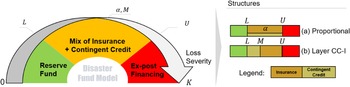
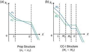


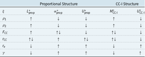


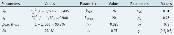
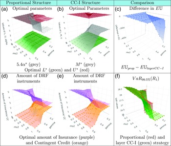


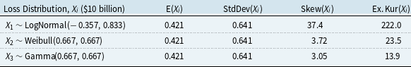


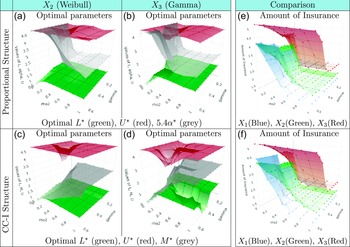

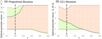


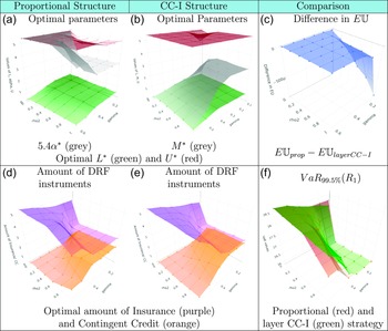

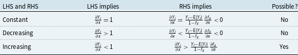
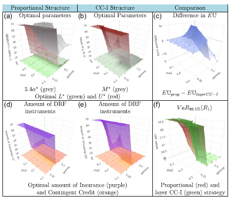


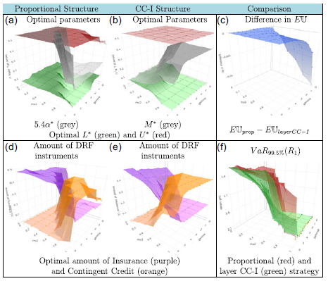

 Open access