2.1. Hydrology model

We apply a 1-D (depth-integrated) hydrology model to the terminal 60 km of the Sermeq Avannarleq flowline to compute subglacial hydraulic head. We conceptualize the glacier hydrologic system as having perfect connectivity between the englacial and subglacial hydrologic systems (i.e. small hydraulic resistance). The assumption of hydraulic equilibrium between the englacial and subglacial systems is reasonable for capturing the seasonal timescale behavior of the glacier hydrologic system. In this conceptual model the subglacial hydraulic head is equivalent to the local englacial water-table elevation, h _e. We therefore use the terms ‘subglacial hydraulic head’ and ‘englacial water-table elevation’ interchangeably. Conduits, which operate at the ice/bed interface, whose geometry evolves through time, control the horizontal water discharge, Q, within the glacier hydrologic system (Fig. 2). Thus, h _e varies in time and space due to variable conduit inflow and outflow as well as dynamic changes in conduit storage. As this model only has one horizontal layer (or ‘component’) representing both the englacial and subglacial systems, it can be viewed as a simplification of more advanced multicomponent models that parameterize the supraglacial, englacial, subglacial and groundwater hydrology components independently (Reference Flowers and ClarkeFlowers and Clarke, 2002; Reference Kessler and AndersonKessler and Anderson, 2004). As a consequence of not explicitly representing the supraglacial hydrologic system and the hydraulic retention time therein (i.e. firn; Reference Fountain and WalderFountain and Walder, 1998), surface ablation is routed instantly to the top of the englacial water table. By enforcing water conservation, the rate of change in hydraulic head (or englacial water-table elevation) at a given node along the flowline may be calculated from four terms: (1) external meltwater input, I (via both surface and basal ablation per unit area), multiplied by the flowband cross width, w, (2) internal meltwater generation due to viscous melt within the conduit, , (3) horizontal divergence of conduit discharge, ∂Q/∂x, and (4) changes in conduit storage volume (per unit length along the flowline) through time, ∂S _c/∂t:

(1)

where φ is the bulk ice porosity at a given node. With w = 1, Equation (1) describes the flow per unit width along the flowline. Assuming the ice behaves like a fractured rock-type aquifer rather than a porous medium-type aquifer, this bulk ice porosity (or ‘macro-porosity’) is taken to represent the fractional volume occupied by fully connected surfaceto-bed discrete water-storage elements (i.e. the lumped fractional volumes of surface and basal crevasses, conduits, moulins, etc.; Reference Flowers and ClarkeFlowers and Clarke, 2002). The geometry of these discrete water-storage elements remains unspecified (Reference Kessler and AndersonKessler and Anderson, 2004). Observed values of bulk ice porosity generally range between 0.004 and 0.013 in alpine glaciers (Reference Fountain and WalderFountain and Walder, 1998). Similar to Reference Kessler and AndersonKessler and Anderson (2004), we take bulk ice porosity as 0.01 and assume it is constant in space and time. We also run simulations with φ = 0.005 and 0.015, the water content range constrained by ice temperature modeling of nearby Jakobshavn Isbræ (Reference Lüthi, Funk, Iken, Gogineni and TrufferLüthi and others, 2002).

Fig. 2.

Schematic of the model variables and coordinate system at a given node. Variable notation table is provided in the Appendix.

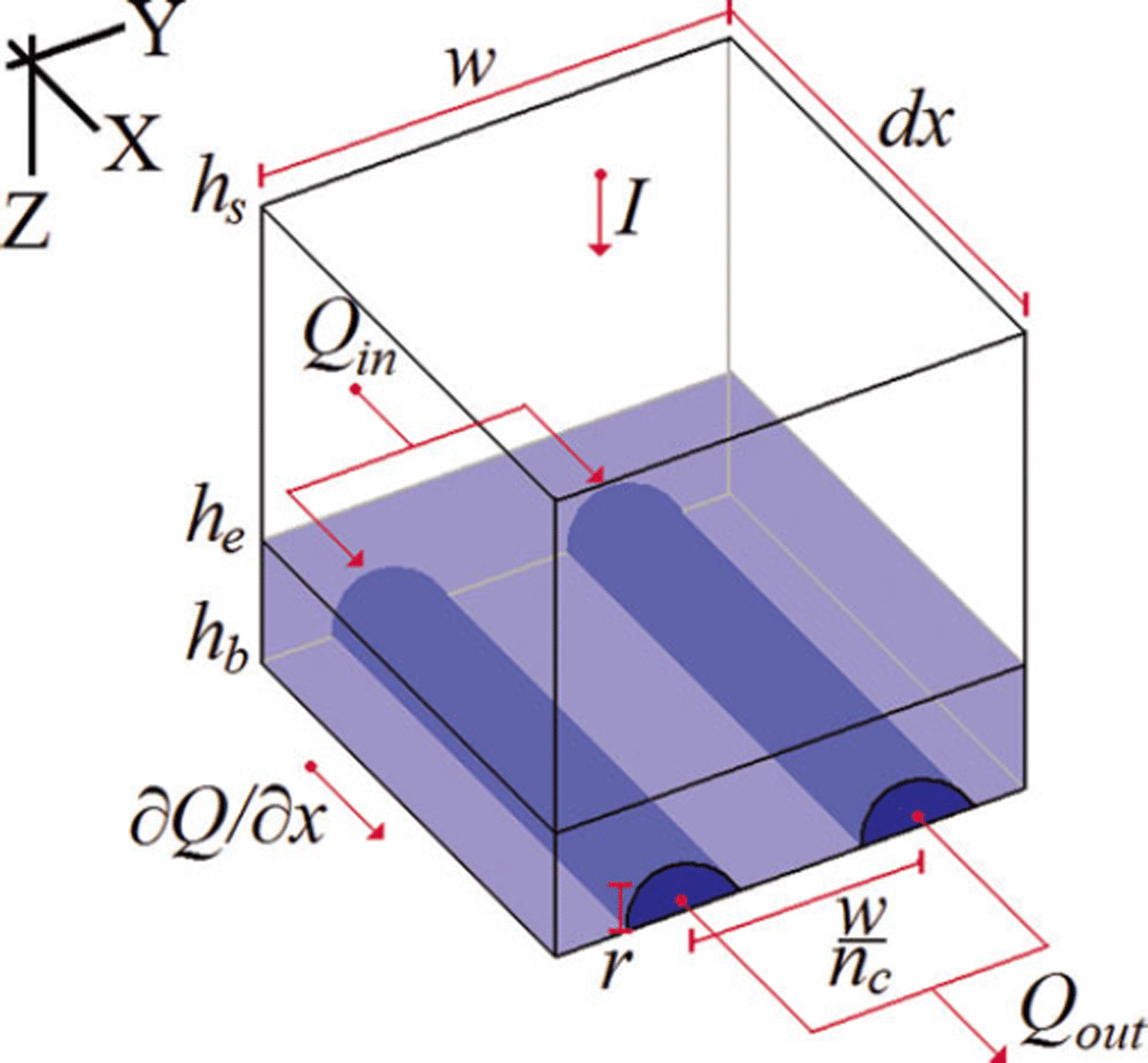
In the conceptual framework of this model, the total water volume stored per unit length along the flowline at a given node within the glacier hydrologic system, S, is the sum of two terms:

(2)

where S _e is the englacial storage volume per unit length and S _c is the subglacial conduit storage volume per unit length. S _e = φwH _e, where H _e is englacial water-column thickness (h _e – h _b). Assuming a semicircular conduit geometry, conduit storage volume per unit length (or total cross-sectional area) can be expressed as a function of conduit radius, r:

(3)

where n _c is the number of conduits per unit width in the cross-flow (y) direction (defined in section 2.1.2).

2.1.1. External meltwater input

At each node along the flowline, external meltwater input, I, occurs as the sum of both surface ablation rate, , and basal ablation rate, , according to

(4)

where F is the fraction of surface meltwater that reaches the englacial water table. This external meltwater input term does not accommodate episodic supraglacial lake drainage events, which can deliver tremendous amounts of water to a single location within the glacier hydrologic system (Reference DasDas and others, 2008). Rather, our interest is in the seasonal timescale response to the annual surface ablation forcing. In the ablation zone, where no firn layer exists, almost all surface meltwater can be expected to reach the glacier hydrologic system. In the accumulation zone, however, meltwater must percolate vertically through the snowpack and firn. As a result of temporary storage or refreezing during this percolation, only a fraction of surface meltwater production reaches the glacier hydrologic system (Reference Pfeffer, Meier and IllangasekarePfeffer and others, 1991; Reference Fountain and WalderFountain and Walder, 1998; Reference Janssens and HuybrechtsJanssens and Huybrechts, 2000). We approximate the englacial entry fraction based on the ratio of annual surface accumulation, c _s, to annual surface ablation, a _s. This formulation follows Reference Pfeffer, Meier and IllangasekarePfeffer and others (1991), who suggest that a given fraction of the annual accumulation must melt and saturate before runoff occurs, i.e.

(5)

Here F _r is the fraction of surface ablation retained in the firn where annual surface ablation and accumulation are equal. We take F _r as 0.5, which implies that water enters the glacier hydrologic system upstream of the equilibrium line. The along-flowline profile of F varies relatively little when F _r is in the range 0.3–0.7 (Fig. 3).

Fig. 3.

(a) Observed annual surface accumulation, c _s (Reference BurgessBurgess and others, 2010), and ablation, a _s (Reference Fausto, Ahlstrøm, van As, Bøggild and JohnsenFausto and others, 2009), versus distance upstream. (b) Englacial entry fraction, F, versus distance upstream with variable values of retention fraction, F _r. Vertical dashed lines denote the locations of JAR2, Swiss Camp and the equilibrium line. (c) Englacial entry fraction (with F _r = 0.5) over the observed range of c _s and a _s values.

We interpolate along-flowline annual surface accumulation, c _s, from a previously compiled dataset (Reference BurgessBurgess and others, 2010). Annual surface ablation, a _s, is taken as a function of elevation, based on previous in situ observations (Reference Fausto, Ahlstrøm, van As, Bøggild and JohnsenFausto and others, 2009), i.e.

(6)

where γ is the present-day ablation gradient (Δa _s/Δh _s, taken as 0.00372; Reference Fausto, Ahlstrøm, van As, Bøggild and JohnsenFausto and others, 2009) and is the equilibrium-line altitude (ELA, taken as 1125 m) and is the annual surface ablation at the ELA (taken as 0.4 m). Annual surface ablation is distributed through time to yield a surface ablation rate, , using a sine function to represent the melt-season solar insolation history (cf. Reference Pimentel and FlowersPimentel and Flowers, 2010):

(7)

where j is a given Julian date (JD), j _o is the JD of melt onset (estimated as j _o = 0.0183h _s + 114), and D is the duration of the melt season (the JD of melt cessation is similarly estimated as j _c = −0.0183h _s+248). While these idealized dates of melt onset and cessation lie within the observed range, this function likely underestimates the date of peak melt, which usually occurs closer to the end of the melt season (Fig. 4).

Fig. 4.

The modeled time–space distribution of surface ablation rate,. Vertical dashed lines denote the locations of JAR2, Swiss Camp and the equilibrium line.

The rate of basal ablation, , is calculated as

(8)

where Q _d and Q _f are the heat input due to deformational (strain) and frictional heating, respectively, Q _g is the geothermal flux, ρ _i is the density of ice (917 kg m⁻³) and L is the latent heat of fusion (333 550 J kg⁻¹). We assume a geothermal flux of 57 m W m⁻² along the entire flowline (Reference Sclater, Jaupart and GalsonSclater and others, 1980). We also assume that deformational heating is concentrated at the ice/bed interface where it contributes to basal ablation (Reference HookeHooke, 2005). The lack of vertical resolution in the single-component hydrology model also necessitates that internally produced meltwater is routed instantaneously to the bed (Reference Flowers, Marshall, Björnsson and ClarkeFlowers and others, 2005). Deformational and frictional heating are calculated as

(9)

where τ _b is taken as the basal gravitational driving stress, is depth-averaged deformational ice velocity and u _b is basal sliding velocity (Reference HookeHooke, 2005). Both τ _b and are calculated according to the shallow-ice approximation using the flow-law parameter for ice defined in section 2.1.4. As this glacier hydrology model is not currently coupled to an ice flow model that incorporates transient basal sliding velocities, we simply parameterize u _b as 15 m a⁻¹ throughout the ablation zone. Based on observations, this basal sliding velocity can be regarded as characteristic of the Sermeq Avannarleq ablation zone (see Colgan and others, in preparation). First-order calculations suggest that Q _f and Q _g are small compared with Q _d, which makes Q _d the main control on basal ablation.

With a mean value of 3.3 cm (std dev. 1.6 cm) in the ablation zone, annual basal ablation is a very small fraction of annual surface ablation. Beneath the km 7 icefall, however, steep surface slopes produce a strong deformational heat flux, which results in annual basal ablation of 9.3 cm. In comparison, annual surface ablation at the icefall is ∼3.5 m. These annual basal ablation values are small compared with those estimated for Jakobshavn Isbræ, where deformational heating alone is capable of producing >0.5 m of meltwater annually (Reference Truffer and EchelmeyerTruffer and Echelmeyer, 2003). Unlike surface ablation, basal ablation is distributed evenly throughout the year. We neglect submarine basal ablation at the ice/ocean interface, as hydraulic head is prescribed as sea level within the ice tongue.

2.1.2. Conduit discharge

Horizontal divergence of conduit discharge, ∂Q/∂x, is the along-flowline gradient in conduit discharge, Q. For sub-glacial conduits, where Reynolds numbers are expected to be large, we calculate discharge based on the Darcy–Weisbach equations for turbulent flow in conduits (e.g. Reference RöthlisbergerRöthlisberger, 1972; Reference NyeNye, 1976; Reference Spring and HutterSpring and Hutter, 1982; Reference Flowers, Björnsson, Pálsson and ClarkeFlowers and others, 2004; Reference Pimentel and FlowersPimentel and Flowers, 2010). As we assume perfect connectivity between the subglacial and englacial systems and that conduits are located at the ice/bed interface, conduit discharge is dependent on the local hydraulic-head gradient, ∂h _e/∂x:

(10)

where g is gravitational acceleration (9.81 m s⁻²), f is a friction factor, D _h is the effective hydraulic diameter, r is the conduit radius, n _c is the number of conduits per meter in the cross-flow direction and w is the flowband cross width. We assume a friction factor of 0.05, which is appropriate for turbulent flow in rough-walled pipes, where the amplitude of the wall roughness elements is ∼0.02 times the pipe diameter (Reference MoodyMoody, 1944). To assess model sensitivity, we also present a simulation in which f is taken as 0.01.

We approximate the observed arborescent nature of subglacial conduit systems (Reference Fountain and WalderFountain and Walder, 1998) within the framework of our flowline model by making the number of conduits per unit width, n _c, in the cross-flow (y) direction an exponential function of distance upstream from the terminus, x:

(11)

where is the number of conduits per unit width at the terminus (taken as 0.005 or 200 m between conduits) and a is a glacier hydrology length scale controlling the rate of increase in number of conduits per unit width (or the rate of decrease in spacing between conduits) with distance upstream. At any flowline position, the subglacial hydrologic system is represented as a set of non-interacting parallel conduits, with a conduit spacing given by Equation (11).

As disequilibrium between the forces promoting conduit opening and closure is permitted in the model (discussed in section 2.1.4), we must constrain conduit radii between reasonable maximum and minimum dimensions to prevent implausible feedbacks (i.e. permanent closure and unrestricted growth). The need to impose these boundaries may be attributed to the intrinsic limitations of a simplified 1-D hydrologic model. The evolving geometry of the subglacial hydrologic system can only be represented accurately with a higher-dimensional model that allows for flow divergence (convergence) away from (towards) highly conductive conduits. A model that incorporates these processes can in principle simulate conduit geometry without prescribed upper and lower bounds for conduit radii. Higher-dimensional modelling would also benefit from a more precise characterization of the bedrock geometry throughout our study area.

Similar to conduit spacing, we also parameterize maximum conduit radius, r _max, as an exponential function of distance upstream from the terminus:

(12)

where is the maximum permissible conduit radius at the terminus (arbitrarily taken as 2 m) and a is the same glacier hydrology length scale as in Equation (11), which controls the rate of decrease in maximum conduit radius with distance upstream (r _min is taken as 10% of r _max).

On the assumption that the total conduit storage volume per unit length, S _c, at a given position along the flowline reflects the integrated annual external meltwater input per unit width that enters the glacier hydrologic system upstream of that position (∫ I · dx), we can approximate the glacier hydrology length scale, α, as the length scale of the along-flowline ∫ I · dx profile. A qualitative assessment suggests that α = 20 km renders an along-flowline S _c profile that approximates the ∫ I · dx profile better than α = 10 or 30 km (Fig. 5). Thus, we take α = 20 km as the glacier hydrology length scale. Together, Equations (11) and (12) capture the essence of an arborescent conduit network, namely the decrease in both conduit spacing and conduit radius with distance upstream (Fig. 6). There are, however, an infinite number of combinations of conduit spacing and radius values that may yield a given discharge, and neither parameter is tightly constrained by field observations. Thus, our maximum and minimum conduit radii may not necessarily reflect actual limits found in nature; they merely reflect limits that, together with the conduit spacing relation we have imposed, lead to reasonable values for the overall transmissivity of the conduit system.

Fig. 5.

(a) Total annual external meltwater input per unit width entering the glacier hydrologic system upstream of a given position (∫ I · dx). (b) Maximum conduit radius, r _max. (c) Conduit spacing in the across-flow direction, n _c. (d) Total conduit storage volume per unit length, S _c. Line color varies with glacier hydrology length scale, α. Vertical dashed lines denote the locations of JAR2, Swiss Camp and the equilibrium line.

Fig. 6.

Schematic of the arborescent approximation of the conduit network: number of conduits (rounded to nearest integer) and maximum conduit diameter, 2r (5 times exaggerated), versus distance upstream when α = 20 km. Horizontal dashed lines denote the locations of JAR2, Swiss Camp and the equilibrium line.

2.1.3. Meltwater generation in conduits

At each node along the flowline, meltwater is generated within the conduits as a consequence of the dissipation of the heat generated by viscous friction in the water; this heat is instantaneously conducted to conduit walls (Reference NyeNye, 1976). The rate at which water is produced by internal melt, _m, in units of mass per length per time at a given node, is a function of conduit discharge, Q, local hydraulic-head gradient, ∂h _e/∂x, and the latent heat of fusion of ice, L:

(13)

2.1.4. Conduit volume

As the conduits grow and shrink at each node along the flowline, the local conduit storage volume per unit length, S _c (or total cross-sectional area), changes. Conduit storage volume grows through two processes: (1) the volume per unit length created by the ice removed through internal meltwater generation (, where is calculated according to Equation (13)), and (2) deformational opening, which occurs when water pressure, P _w (defined as ρ _w gH _e), exceeds ice pressure, P _i (defined as ρ _i gH _i). Conversely, conduit storage volume only decreases through deformational closure when P _i > P _w. Thus, our model assumes that deformational opening of conduits can occur in response to high subglacial water pressures (Reference NyeNye, 1976; Reference NgNg, 2000; Reference ClarkeClarke, 2003). As we are assuming perfect connectivity between the subglacial and englacial systems, the basal water pressure both inside and outside the conduits may be regarded as equivalent. This implicitly discounts the possibility of ‘leakage’ of high water pressures from the conduit system to adjacent regions (Reference Bartholomaus, Anderson and AndersonBartholomaus and others, 2008). As basal ice temperature in the ablation zone is likely at the pressure-melting point (Reference Phillips, Rajaram and SteffenPhillips and others, 2010), we do not consider conduit closure through refreezing of water within the conduits. The processes that govern the transient rate of change of conduit storage volume per unit length, ∂S _c/∂t, can be expressed as (Reference NyeNye, 1976)

(14)

where A is the temperature-dependent flow-law parameter (Reference Huybrechts, Letréguilly and ReehHuybrechts and others, 1991) and n is the Glen’s law exponent (n = 3). We enhance the temperature-dependent flow-law parameter by a factor of three to account for softer Wisconsinan basal ice (Reference ReehReeh, 1985; Reference PatersonPaterson, 1991), which comprises the bottom ∼20% of the ice column along the flowline (Reference HuybrechtsHuybrechts, 1994).

As recent thermodynamic modeling suggests that basal ice throughout the ablation zone of the Sermeq Avannarleq flowline is at the pressure-melting point (Reference Phillips, Rajaram and SteffenPhillips and others, 2010), we calculate basal ice temperature, T _i, downstream of the equilibrium line as

(15)

where β is the change in melting point with ice thickness (taken as 8.7 × 10⁻⁴ K m⁻¹;Reference PatersonPaterson, 1994). In the accumulation zone, where downward vertical ice velocities are expected to produce cold basal ice temperatures, we simply prescribe basal ice temperature as 268 K. This is the basal ice temperature predicted just upstream of the equilibrium line by recent thermodynamic modeling (Phillips and others, unpublished information). We linearly transition from pressure-melting point basal ice temperatures in the ablation zone to the cold basal ice temperature of the accumulation zone between the equilibrium line and 5 km upstream of the equilibrium line. The resultant basal ice temperature profile is consistent with the notion that meltwater percolation rapidly warms the ice below the equilibrium line and captures the essence of Sermeq Avannarleq basal ice temperature profiles produced by Phillips and others (unpublished information; Fig. 7).

Fig. 7.

(a) Modeled (black; see Colgan and others, in preparation) and observed (grey; Reference Scambos and HaranScambos and Haran, 2002) ice surface elevation, h _s, and observed bedrock topography, h _b (Reference Bamber, Layberry and GogineniBamber and others, 2001; Reference Plummer, Gogineni, van der Veen, Leuschen and LiPlummer and others, 2008). (b) Estimated basal ice temperature, T _i. Vertical dashed lines denote the locations of JAR2, Swiss Camp and the equilibrium line.

2.2. Datasets and boundary conditions

This hydrology model employs several observational data-sets. Annual surface accumulation and annual surface ablation profiles were obtained from previously compiled datasets (Reference Fausto, Ahlstrøm, van As, Bøggild and JohnsenFausto and others, 2009; Reference BurgessBurgess and others, 2010). Both these ice-sheet-scale surface climatology datasets use models to interpolate between in situ observations, including the four Greenland Climate Network (GC-Net) AWSs along the Sermeq Avannarleq flowline (Reference Steffen and BoxSteffen and Box, 2001). To define ice geometry, we use a modeled ice surface elevation (h _s) profile (see Colgan and others, in preparation), which compares well with the profile interpolated from a DEM of the Greenland ice sheet derived from satellite altimetry enhanced by photoclinometry (Reference Scambos and HaranScambos and Haran, 2002; Fig. 7). A coarse-resolution bedrock elevation (h _b) dataset is available along the entire flowline (Reference Bamber, Layberry and GogineniBamber and others, 2001). While this dataset has nominal 5 km horizontal resolution, actual resolution is dependent on the spacing of airborne flight-lines, and thus varies spatially and can exceed 5 km. A finer-resolution dataset (nominally 750 m) is available for the terminal 40 km of the flowline (Reference Plummer, Gogineni, van der Veen, Leuschen and LiPlummer and others, 2008).

Equipotential englacial hydraulic-head gradients are theoretically ∼11 times more sensitive to ice surface slopes than bedrock slopes (Reference ShreveShreve, 1972). Thus, first-order ice surface slope (i.e. regional or ∼10 ice thicknesses) may be expected to govern the first-order geometry of subglacial flow direction. For example, the water beneath Swiss Camp can be expected to travel ∼30 km to the ice-sheet margin on an azimuth of ∼279° (i.e. following regional ice surface slope; dashed line in Fig. 1). By forcing subglacial water to flow along the ice-dynamic flowline to the margin (i.e. following steepest local or ∼1 ice thickness surface slope), subglacial water is routed ∼48 km on an azimuth of ∼225°. This artificially reduces the hydraulic-head gradient, ∂h _e/∂x, by artificially increasing dx. To compensate for this we use simple trigonometry to project the dynamic flowline on the hydrologic coordinates, correcting dx values on a node-bynode basis, and thereby maintaining realistic ∂h _e/∂x values along the length of the flowline.

We apply first-type (specified head) Dirichlet boundary conditions to hydraulic head, h _e. From km0 to 2, the tidewater terminus, h _e is prescribed as sea level (i.e. h _e = 0 m). We use the cold-to-warm basal ice temperature transition at the equilibrium line (km 51) to approximate the upstream limit of the glacier hydrologic system. We impose a no-flux boundary that extends upwards from the bedrock beneath the equilibrium line to the ice surface at 11 times the local surface slope. This is the steepest theoretical gradient that water traveling through the ice sheet could be expected to take in order to reach the bed at the cold-to-warm basal ice temperature transition beneath the equilibrium line (Reference ShreveShreve, 1972). Thus, upstream of the equilibrium line, there is a portion of the glacier hydrologic system that behaves as a ‘perched’ aquifer (i.e. underlain by cold ice). In this ∼4 km portion of the flowline, we assume that ice temperature is sufficiently heterogeneous to allow the persistence of englacial conduits (Reference Catania and NeumannCatania and Neumann, 2010). We treat the discharge of these conduits in an identical manner to the conduits downstream of the equilibrium line, except we suspend the processes that govern the transient rate of change of conduit storage volume, ∂S _c/∂t, and prescribe conduit radii as constant (5 cm). We assume that any water entering the ice upstream of the intersection of the perched aquifer and the ice surface refreezes, although we do not perform a full enthalpy solution to incorporate this process as a transient flux. We also assume that basal ablation is zero beneath the cold basal ice in the accumulation zone. The glacier hydrologic system is therefore fully transient over the 49 km between the equilibrium line (km 51) and the tidewater terminus (km 2).

The differential equations describing transient hydraulic head, ∂h _e/∂t, were discretized in space using first-order finite-volume methods (dx = 500 m) with hydraulic head, h _e, at cell centers and fluxes, Q, at cell edges. The semi-discrete set of ordinary differential equations coupled at the computational nodes was then solved using ‘ode15s’, the stiff differential equation solver in MATLAB R2008b, with a 1 day time-step.

4.1. Hydrology model

Based on the absolute value of flotation fraction, as well as qualitative features in the annual hydraulic-head cycle (i.e. a positive phase followed by a negative phase with no significant change during the winter), we conclude that the relatively simple one-component 1-D hydrology model produces a reasonable annual hydrologic cycle along the terminal 60 km of the Sermeq Avannarleq flowline. The modeled hydraulic head oscillates close to flotation throughout the ablation zone of the Sermeq Avannarleq flowline. The suggestion of a relatively high englacial water table is consistent with previous in situ observations of flotation fractions between 0.79 and 1.05 in the Paakitsoq area (69.5° N, 50.0° W; Reference Thomsen and OlesenThomsen and Olesen, 1991) and between 0.95 and 1.00 in Jakobshavn Isbræ (69.2° N, 48.7° W; Reference Iken, Echelmeyer, Harrison and FunkIken and others, 1993; Reference Lüthi, Funk, Iken, Gogineni and TrufferLüthi and others, 2002). The high modeled flotation fraction along the flowline is due to the dependence of conduit conductivity and discharge on the relative difference between water and ice pressures. Sufficiently high hydraulic head is needed to overcome basal ice pressure and open the conduits. Once open, conduits draw down hydraulic head until reaching a threshold below which hydraulic head is no longer sufficient to counteract basal ice pressure and keep the conduits open. The conduits subsequently close, achieving their minimum prescribed radius, r _min, leaving large amounts of residual water stored in the glacier.

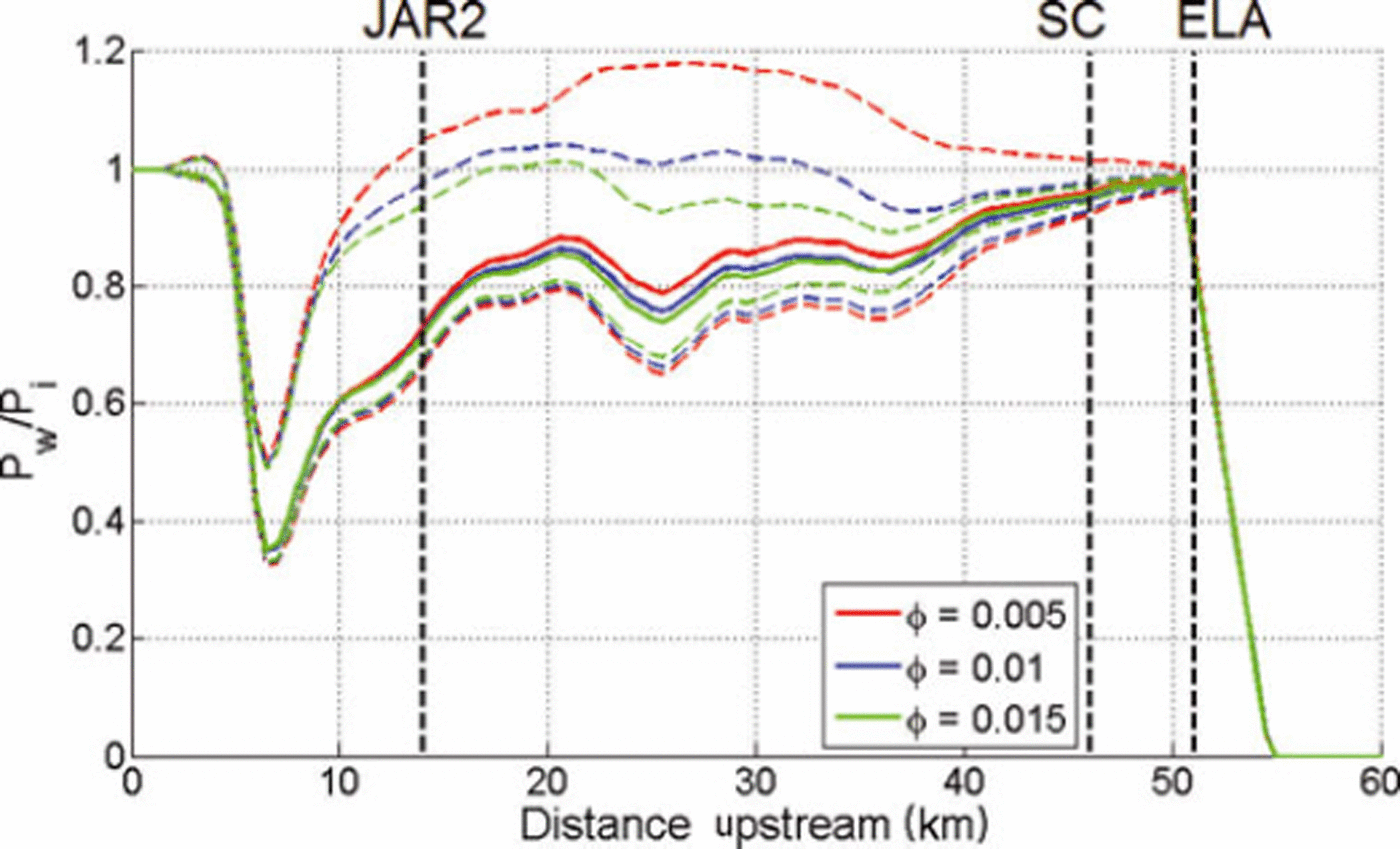
Model runs in which bulk ice porosity, φ, is taken as 0.005 and 0.015 return very similar along-flowline profiles of mean annual flotation fraction (Fig. 11). Thus, a relatively high hydraulic head is likely an inherent feature of a glacier hydrologic system drained solely by conduits. The alongflowline profile of maximum flotation fraction is, however, higher (lower) in the lower (higher) bulk ice porosity simulation. Thus, as currently parameterized, the magnitude of ∂h _e/∂t is a function of bulk ice porosity. When φ = 0.005, flotation fraction values are unrealistically high in the vicinity of km 25 (∼1.2 which is conducive to artesian springs). Bulk ice porosity values as low as 0.0005 have been postulated for alpine glaciers (Reference Humphrey, Raymond and HarrisonHumphrey and others, 1986). Our sensitivity analysis suggests that increased water storage at the bed must be invoked to produce realistic flotation fraction values when φ ≪ 0:01. At present, our single-component model does not explicitly incorporate the water storage volume created at the ice/bed interface by vertical uplift of the ice sheet (cf. Reference Pimentel and FlowersPimentel and Flowers, 2010). Due to this limitation a portion of the bulk ice porosity can be assumed to represent the storage volume of discrete voids at the ice/bed interface. In reality, the storage volume at the ice/bed interface is likely a function of hydraulic head, rather than constant in space and time as we have implicitly assumed by using constant porosity.

Fig. 11.

Mean annual flotation fraction, P _w/P _i, versus distance upstream for various values of bulk ice porosity, φ. Dashed curves represent annual maximum and minimum values. Vertical dashed lines denote the locations of JAR2, Swiss Camp and the equilibrium line.

The model inference of year-round subglacial conduit storage along certain portions of the flowline (km 16–25 and 42–50) is supported by limited observations of the persistence of some englacial hydrology features through the winter in the Sermeq Avannarleq ablation zone (Reference Catania and NeumannCatania and Neumann, 2010). The sharp model transitions between year-round and seasonally active conduit storage appear to be due to slight changes in the along-flowline gradient in local hydraulic head, ∂h _e/∂x; subglacial conduit storage volume per unit length, S _c, is proportional to the magnitude of (∂h _e/∂x)^1.5. When a bedrock topography that increases monotonically upstream is imposed, the pockets of year-round subglacial conduit storage form in the same location as when the observed bedrock topography is imposed (Animation 2). As short stretches of year-round subglacial conduit storage appear to form downstream of stretches of relatively steep ice surface topography, we speculate that the alongflowline gradient in ice surface elevation, dh _s/dx, influences the along-flowline gradient in local hydraulic head, ∂h _e/∂x, and hence the location of year-round subglacial conduit storage. When an ice surface topography with sinusoidal undulations (25 m amplitude and 10 km wavelength) is imposed, the pockets of year-round subglacial conduit storage tend to form beneath portions of the flowline with the steepest ice surface slopes (Animation 3). Along-flowline gradients in flotation fraction, P _w/P _i, as a result of ice surface topography may also have an influence in the location of year-round subglacial conduit storage. Maintaining year-round subglacial conduit storage through deformational opening, however, could only be expected along portions of the flowline where water pressure exceeds ice pressure year-round. The time–space distribution of modeled flotation fraction suggests that this only occurs in the tidewater tongue (km 0–2; Fig. 9). The model inference that portions of the subglacial conduit storage system may overwinter at the base of the Greenland ice sheet to be reactivated the following melt season differs slightly from previous alpine glacier work, which suggests a new channelized subglacial hydrologic system migrates up-glacier from the terminus each melt season (Reference Hubbard and NienowHubbard and Nienow, 1997).

Animation 2.

Same as Animation 1 except with a modified bedrock topography that increases monotonically upstream. Full movie available at http://www.igsoc.org/hyperlink/10J154_Animation2.mov.

Animation 3.

Same as Animation 2 except with a sinusoidal pattern (25 m amplitude and 10 km wavelength) imposed on ice surface topography and basal ablation actively disabled. Full movie available at www.igsoc.org/hyperlink/10J154_Animation3.mov.

During the period of peak decreasing hydraulic head at Swiss Camp (i.e. JD 300 or 325, depending on f parameterization; Fig. 10) the conduits draw down hydraulic head with the efficiency of a semicircular conduit 40 cm in diameter spaced every 20 m and operating at basal ice and water pressure (i.e. n _c = 0.050 m and r = 0.20 m). Similarly, during the period of peak decreasing hydraulic head at JAR2 (∼JD 180) the conduit system is parameterized to discharge water with the efficiency of a semicircular conduit 1.98 m in diameter spaced every 100 m operating at basal ice and water pressure (n _c = 0.010 m and r = 0.99 m). Although our parameterized conduit system appears to be reasonable, a lack of field observations makes this configuration speculative. The choice of conduit friction factor, f, which is a measure of resistance (discharge is inversely related to f), appears to influence the timing, but not magnitude, of negative ∂h _e/∂t values (Fig. 10). A smaller value of f propagates the perturbation in hydraulic-head gradient responsible for conduit opening upstream more quickly than a larger value of f.

Assuming a bulk ice porosity of 0.01, and that the modeled glacier hydrologic cycle is in quasi-steady state, the mean residence time, t _res, of water in the flowline can be calculated as ∼2.2 years, when w = 1 m, according to

(16)

where ∫ S · dx is the total flowline modeled water storage (annual mean ≈45 000 m³) and ∫ Iw · dx is the total flowline prescribed external water input (annual mean ≈20 000 m³ a⁻¹;Fig. 8). The integral notation (∫ · dx) refers to integration of continuous values over the entire length of flowline (i.e. all x values). Assuming bulk ice porosities of 0.005 and 0.015, the mean residence times are ∼1.1 and 3.3 years, respectively. This relatively short residence time suggests that the glacier hydrologic system can be expected to respond to external meltwater forcings on a relatively short timescale (i.e. years rather than decades).

4.2. Relevance to basal sliding

In section 1 we reviewed the notion that variations in basal sliding velocity can be attributed to variations in the rate of change of glacier water storage (i.e. dS/dt) in alpine glaciers (Reference Kamb, Engelhardt, Fahnestock, Humphrey, Meier and StoneKamb and others, 1994; Reference Fountain and WalderFountain and Walder, 1998; Reference AndersonAnderson and others, 2004; Reference Bartholomaus, Anderson and AndersonBartholomaus and others, 2008). This conceptual model of basal sliding has recently been extended to the Greenland ice sheet (Reference Bartholomew, Nienow, Mair, Hubbard, King and SoleBartholomew and others, 2010). Below we present both remotely sensed and in situ velocity data from the Sermeq Avannarleq flowline that suggest that observed periods of enhanced basal sliding generally correspond to modeled periods of positive rates of change in glacier water storage (or increasing hydraulic head), while periods of reduced basal sliding conversely correspond to modeled periods of negative rates of change in glacier water storage (or decreasing hydraulic head).

Given the proximity of Sermeq Avannarleq to Jakobshavn Isbræ, multiple 2005 and 2006 interferometric synthetic aperture radar (InSAR)-derived ice surface velocity profiles are available for the terminal 60 km of the Sermeq Avannarleq flowline (Reference Joughin, Das, King, Smith, Howat and MoonJoughin and others, 2008). Linear interpolation between these profiles yields a time–space velocity plot (Fig. 12). While summer velocities are not available upstream of km 22, the region around JAR2 exhibits a distinct annual velocity cycle. This cycle consists of a summer speed-up event, in which velocities exceed winter velocity, followed by a fall slowdown event, in which velocities decrease to lower than winter velocity. These observed velocity anomalies may be interpreted as periods of enhanced and suppressed basal sliding that qualitatively correspond to periods of modeled increasing and decreasing hydraulic head.

Fig. 12.

Annual ice surface velocity cycle along the terminal 60 km of the Sermeq Avannarleq flowline (color bar saturates at 175 m a⁻¹). Dotted black lines indicate individual InSAR velocity profiles. Vertical dashed lines denote the locations of JAR2, Swiss Camp and the equilibrium line.

High-frequency differential GPS measurements have been acquired at Swiss Camp since June 1996, providing daily resolution of the annual ice surface velocity cycle for the last 12 years (Reference Larson, Plumb, Zwally and AbdalatiLarson and others, 2001; Reference Zwally, Abdalati, Herring, Larson, Saba and SteffenZwally and others, 2002; Fig. 13). In accordance with the InSAR observations, these in situ GPS observations reveal that the ice at Swiss Camp also experiences a summer speed-up event, in which ice velocities increase above winter velocities, followed by a fall slowdown event, in which ice velocities decrease below winter velocities. The summer speed-up event varies in peak magnitude and timing over the 12 year record, presumably due to variable surface climatology and meltwater forcing, as well as local supraglacial lake drainage events. While the model is not forced with an observed melt history, the modeled period of increasing hydraulic head (i.e. JD 150–200) generally matches the timing of the observed speed-up event. The observed slowdown event, however, follows the observed speed-up event in relatively quick succession. The modeled peak in decreasing hydraulic head lags the modeled peak in increasing hydraulic head by 125–150 days (depending on the value of f; Fig. 10).

Fig. 13.

Observed GPS annual velocity cycle at Swiss Camp over the 1996–2008 period.

We speculate that this apparent delay in the negative ∂h _e/∂t phase, which is due to a delay in opening the upstream conduits, is a consequence of 1-D hydrological modeling. A two-dimensional (2-D; xy) hydrological model would better capture changes in englacial water-table gradient at Swiss Camp by allowing conduit discharge both parallel and perpendicular to the ice-dynamic flowline. Presently, by forcing water to flow along the entire ice-dynamic flowline to the terminus, the 1-D model essentially requires the perturbation in local hydraulic head gradient that initiates conduit opening to slowly migrate from the terminus upstream to Swiss Camp. In reality, the glacier hydrologic system near Swiss Camp is governed by both along- and across-flow hydraulic head gradients (∂h _e/∂x and ∂h _e/∂y respectively). A 2-D (xy) model would better represent the influence of bedrock topography on subglacial discharge, by allowing subglacial discharge to concentrate in topographic low points (Reference ShreveShreve, 1972; Reference Flowers, Marshall, Björnsson and ClarkeFlowers and others, 2005). Due to this concentration of discharge, 2-D models are inherently more capable of developing larger and more efficient conduits than 1-D models.

Based on the qualitative agreement between observations of a strong annual ice velocity cycle and the modeled annual glacier hydrologic cycle, we propose that the terminal 50 km of the Greenland ice sheet’s Sermeq Avannarleq flowline behaves akin to an alpine glacier, whereby the summer speed-up event is caused by inefficient subglacial drainage and positive rates of change of glacier water storage (i.e. dS/dt> 0, or increasing hydraulic head), while the fall slowdown event reflects the establishment of efficient subglacial drainage and negative rates of change of glacier water storage (i.e. dS/dt<0, or decreasing hydraulic head). A notable departure from the alpine analogy, however, is the model inference that subglacial conduit storage may be capable of overwintering beneath the Greenland ice sheet to be reactivated the following melt season, rather than migrating up-glacier from the terminus each melt season as observed in alpine glaciers (Reference Hubbard and NienowHubbard and Nienow, 1997). The recovery of both basal sliding velocities and rates of change of hydraulic head, ∂h _e/∂t, to winter values shortly after the fall slowdown, suggests that the glacier hydrologic system is capable of repressurizing to maintain winter sliding. Presumably, this occurs by: (1) a reduction in transmissivity due to conduit closure and (2) continued meltwater input, largely via basal ablation due to geothermal, frictional and deformation (strain) heat fluxes rather than internal meltwater generation,.