


1. Introduction
Transient radio emission is a signature of some of the most energetic and interesting events in our Universe: from stellar explosions (Weiler et al. Reference Weiler, Panagia, Montes and Sramek2002) and compact object mergers (Hallinan et al. Reference Hallinan2017) to tidal disruption and accretion around supermassive black holes (Zauderer et al. Reference Zauderer2011). These dynamic events happen in extreme physical conditions and hence let us test fundamental physics such as mechanisms for magnetic field generation, particle acceleration, the strong-field gravity regime (Kramer et al. Reference Kramer2021) and the cosmological star formation history (Tanvir et al. Reference Tanvir2009; Chandra et al. Reference Chandra2010). They also act as probes of the interplanetary (Jokipii Reference Jokipii1973), interstellar (Rickett Reference Rickett1990) and intergalactic media (Zhou et al. Reference Zhou, Li, Wang, Fan and Wei2014), giving us insight into the structure and composition of the Universe on all scales.
Transient events have played an important role in astronomy since its early days. For example, there are numerous records of ‘guest stars’ by Chinese astronomers in the first century of the Common Era (Stephenson & Green Reference Stephenson and Green2002), some of which were later established to be historical supernovae. In Europe, Tycho Brahe’s detailed observations of SN 1572 were an important step forward in challenging the Aristotelian/Ptolemaic paradigm of the ‘unchanging heavens’ (Hinse et al. Reference Hinse, Dorch, Occhionero and Holck2023). In the present era, targeted monitoring and surveys of optical transients have led to major discoveries: perhaps most notably the discovery of the accelerating expansion of the Universe through observations of distant supernovae (Riess et al. Reference Riess1998; Perlmutter et al. Reference Perlmutter1999), which won the 2011 Nobel Prize for Physics. Most recently, the detection of a gravitational wave transient, a binary black hole merger (Abbott et al. Reference Abbott2016), led to the 2017 Nobel Prize for Physics and opened up the field of multi-messenger transients (Abbott et al. Reference Abbott2017b ).
In contrast to optical and X-ray wavebands, the dynamic radio sky had been relatively unexplored (beyond targeted observations). The notable exception to this was pulsars, the discovery (Hewish et al. Reference Hewish, Bell, Pilkington, Scott and Collins1968) and study (Hulse & Taylor Reference Hulse and Taylor1975) of which have led to two Nobel Prizes, in 1974 and 1993 respectively. Looking beyond pulsars, the general lack of large-scale time domain studies at radio frequencies (until recent times – see Section 4.3) has been largely due to observational limitations: widefield, sensitive surveys with multiple epochs were difficult and time consuming to conduct.
Transient phase space showing radio luminosity versus the product of timescale and observing frequency for different transient source classes, following Cordes et al. (Reference Cordes, Lazio and McLaughlin2004). Note that the luminosity assumes sources are beamed into only 1 sr and no relativistic beaming, which may or may not be appropriate for individual objects, while the timescales are just the observed variability timescales and ignore more constraining limits such as the finite sizes of e.g. stellar sources. For sources with relativistic beaming the true brightness temperature could be significantly lower (e.g. Readhead Reference Readhead1994), while for some stellar sources the true brightness temperature could be significantly higher, as suggested by the arrows. The diagonal lines show contours of brightness temperature, with coherent emitters having
 $T_B\gt10^{12}\,$
K. Adapted from Pietka et al. (Reference Pietka, Fender and Keane2015) and Nimmo et al. (Reference Nimmo2022), with select sources added: the binary neutron star merger GW170817 (Mooley et al. Reference Mooley2018c); LFBOTs (Ho et al. Reference Ho2019; Coppejans et al. Reference Coppejans2020; Ho et al. Reference Ho2020); relativistic TDEs (Mimica et al. Reference Mimica, Giannios, Metzger and Aloy2015; Andreoni et al. Reference Andreoni2022); flare stars/brown dwarfs (Hallinan et al. Reference Hallinan2007; Rose et al. Reference Rose2023; Route & Wolszczan Reference Route and Wolszczan2016; Zic et al. Reference Zic2019); long-period radio pulsars (Caleb et al. Reference Caleb2022; Wang et al. Reference Wang2025d); Galactic Centre radio transients (Hyman et al. Reference Hyman, Lazio, Kassim, Ray, Markwardt and Yusef-Zadeh2005; Wang et al. Reference Wang2021b
); white dwarf pulsars (Pelisoli et al. Reference Pelisoli2023; de Ruiter et al. Reference de Ruiter2025) and long-period transients (Wang et al. Reference Wang2025c
; Lee et al. Reference Lee2025; Wang et al. Reference Wang2021b
; Caleb et al. Reference Caleb2024; Hurley-Walker et al. Reference Hurley-Walker2024, Reference Hurley-Walker2023, Reference Hurley-Walker2022b
; Dong et al. Reference Dong2025b
). In particular we highlight the range of sources from Table 2 that are filling out the centre of this space, straddling the coherent/incoherent divide: long-period radio pulsars are upward-pointing triangles, GCRTs are diamonds, pulsing white dwarf binaries are right-pointing triangles, and long period transients (LPTs) are squares.
$T_B\gt10^{12}\,$
K. Adapted from Pietka et al. (Reference Pietka, Fender and Keane2015) and Nimmo et al. (Reference Nimmo2022), with select sources added: the binary neutron star merger GW170817 (Mooley et al. Reference Mooley2018c); LFBOTs (Ho et al. Reference Ho2019; Coppejans et al. Reference Coppejans2020; Ho et al. Reference Ho2020); relativistic TDEs (Mimica et al. Reference Mimica, Giannios, Metzger and Aloy2015; Andreoni et al. Reference Andreoni2022); flare stars/brown dwarfs (Hallinan et al. Reference Hallinan2007; Rose et al. Reference Rose2023; Route & Wolszczan Reference Route and Wolszczan2016; Zic et al. Reference Zic2019); long-period radio pulsars (Caleb et al. Reference Caleb2022; Wang et al. Reference Wang2025d); Galactic Centre radio transients (Hyman et al. Reference Hyman, Lazio, Kassim, Ray, Markwardt and Yusef-Zadeh2005; Wang et al. Reference Wang2021b
); white dwarf pulsars (Pelisoli et al. Reference Pelisoli2023; de Ruiter et al. Reference de Ruiter2025) and long-period transients (Wang et al. Reference Wang2025c
; Lee et al. Reference Lee2025; Wang et al. Reference Wang2021b
; Caleb et al. Reference Caleb2024; Hurley-Walker et al. Reference Hurley-Walker2024, Reference Hurley-Walker2023, Reference Hurley-Walker2022b
; Dong et al. Reference Dong2025b
). In particular we highlight the range of sources from Table 2 that are filling out the centre of this space, straddling the coherent/incoherent divide: long-period radio pulsars are upward-pointing triangles, GCRTs are diamonds, pulsing white dwarf binaries are right-pointing triangles, and long period transients (LPTs) are squares.

We now know the radio sky is variable on all timescales, from nanoseconds (Hankins et al. Reference Hankins, Kern, Weatherall and Eilek2003) through to months and years (Chandra & Frail Reference Chandra and Frail2012; Zauderer et al. Reference Zauderer, Berger, Margutti, Pooley, Sari, Soderberg, Brunthaler and Bietenholz2013). The past decade has seen many advances in our understanding of radio transients, from the detection of radio emission from a binary neutron star merger (Hallinan et al. Reference Hallinan2017), to the real-time detection of an extreme scattering event (Bannister et al. Reference Bannister, Stevens, Tuntsov, Walker, Johnston, Reynolds and Bignall2016) and the discovery of a new class of long period transients (Hurley-Walker et al. Reference Hurley-Walker2022b ). This review is being written as we prepare for the wave of discoveries that will come in the era of the SKA Observatory (SKAO; Dewdney et al. Reference Dewdney2022), which is expected to begin science verification observations in 2027 and 2029 for the SKA-Low and SKA-Mid telescopes, respectively.Footnote a
1.1. The context for this review
There have been a number of reviews of radio transient surveys, mostly written in anticipation of the advent of the ‘next-generation’ radio telescopes that would enable large-scale time-domain imaging surveys on the path to the SKAO. The first of these is Cordes et al. (Reference Cordes, Lazio and McLaughlin2004) who defined a phase space for the exploration of radio transients (we show an updated version of it in Figure 1), and proposed a metric for the optimisation of radio transients surveys (we discuss and expand on this in Section 4.1), as well as discussing some of the key science cases for the SKAO. When Fender & Bell (Reference Fender and Bell2011) reviewed the field, they considered the time domain radio sky was still relatively unexplored. They highlighted the great potential of the major surveys about to commence on MeerKAT (Jonas et al. Reference Jonas2016), the Australian SKA Pathfinder (ASKAP; Hotan et al. Reference Hotan2021), and other SKAO pathfinder and precursor telescopes, with a particular emphasis on the Low-Frequency Array (LOFAR; van Haarlem et al. Reference van Haarlem2013). However, their predictions were based primarily on the transient rates reported by Bower et al. (Reference Bower, Saul, Bloom, Bolatto, Filippenko, Foley and Perley2007), most of which were later shown to be spurious (Frail et al. Reference Frail, Kulkarni, Ofek, Bower and Nakar2012, see Section 4.3.4).
The next review paper was the product of the ‘Advancing Astrophysics with the Square Kilometre Array’ meeting in Italy in 2014 (Braun et al. Reference Braun, Bourke, Green, Keane and Wagg2015). Fender et al. (Reference Fender, Stewart, Macquart, Donnarumma, Murphy, Deller, Paragi and Chatterjee2015a ) discuss the advantages of radio observations for understanding transient objects and present updated limits on radio transient rates from the untargeted transient surveys available at the time; these rates and limits were crude, owing to the lack of robust large-scale samples and reliable real-time identification of transients. Although not formally a review paper, Mooley et al. (Reference Mooley2016) presents the most comprehensive recent compilation of radio transient surveys and detection rates. The online tableFootnote b has been updated to 2025, and hence serves as a very useful summary of work in this area. We draw on this in our review of the history of radio transient surveys presented in Section 4.3.
Just over twenty years on from Cordes et al. (Reference Cordes, Lazio and McLaughlin2004) there are several major radio transient surveys well underway, with the capability to detect significant numbers of transient sources across the full range of their stated scientific goals. The SKAO will be operational within
 $\sim5\textrm{--}8$
yr, and planning is underway for other future instruments including the next-generation Very Large Array (ngVLA; Murphy Reference Murphy2018) and Deep Synoptic Array (DSA-2000; Hallinan et al. Reference Hallinan2019). Hence, it is timely to do a comprehensive review of this area. We hope it will be useful as a milestone in capturing the state of the field as we enter an era of transformational surveys.
$\sim5\textrm{--}8$
yr, and planning is underway for other future instruments including the next-generation Very Large Array (ngVLA; Murphy Reference Murphy2018) and Deep Synoptic Array (DSA-2000; Hallinan et al. Reference Hallinan2019). Hence, it is timely to do a comprehensive review of this area. We hope it will be useful as a milestone in capturing the state of the field as we enter an era of transformational surveys.
The structure of the paper is as follows. In the rest of this section we outline the scope of the review and define some key terminology. In Section 2, we discuss the key emission mechanisms that cause radio variability and in Section 3 we describe each of the main classes of radio transients. In Section 4, we discuss the motivation for untargeted surveys, and present a history of radio transient surveys. In Section 5, we discuss the main detection methods and approaches for radio transients. In Section 6, we discuss the metrics used to measure variability, and how we characterise the time variable sky. In Section 7, we discuss SKAO-era telescopes and how we can incorporate what we have learned from previous work. Finally, in Section 8, we present the future outlook for the field of radio transients.
1.2. The scope of this review
In this review we will focus on results from interferometers in a synthesis imaging mode (i.e. not single dish or coherent beamforming, although we do discuss those separately), often referred to as ‘image domain’ or ‘slow’ transientsFootnote
c
or similar (also see Section 1.3). Early observations of slow transients using single-dish telescopes (e.g. Spangler, Shawhan, & Rankin Reference Spangler, Shawhan and Rankin1974a
), made detections that were difficult to verify and distinguish from interference (Davis et al. Reference Davis, Lovell, Palmer and Spencer1978). Most recent studies use interferometric imaging at frequencies
 $\lt30\,$
GHz, although very large single-dish telescopes can offer advantages (e.g. Route & Wolszczan Reference Route and Wolszczan2013; Route Reference Route2019). At higher frequencies bolometric imaging arrays are the best option for millimetre surveys (Whitehorn et al. Reference Whitehorn2016; Naess et al. Reference Naess2021).
$\lt30\,$
GHz, although very large single-dish telescopes can offer advantages (e.g. Route & Wolszczan Reference Route and Wolszczan2013; Route Reference Route2019). At higher frequencies bolometric imaging arrays are the best option for millimetre surveys (Whitehorn et al. Reference Whitehorn2016; Naess et al. Reference Naess2021).
For both scientific and technical reasons, this review focuses on astronomical phenomena that show variability at radio wavelengths on timescales of seconds to years. We will discuss the physical processes that cause this variability and summarise the main classes of objects that are detected as variable radio sources. We will also cover radio transients surveys, detection methods and population rates.
To define a clear scope for the paper, we will not discuss the following topics:
-
• Solar, heliospheric, and ionospheric science: The Sun is the brightest radio source in the sky, and was first detected in the early days of radio astronomy (Hey Reference Hey1946). The proximity of the Sun to Earth means we are able to study its radio variability in great detail. Solar radio astronomy typically uses different observational approaches and techniques from the radio transients community. In fact, almost all continuum imaging observations (whether targeted, or untargeted surveys) deliberately avoid the Sun due to the impact on data quality. The main exceptions to this are recent programs that use interplanetary scintillation (IPS) caused by the solar wind (discovered by Clarke Reference Clarke1964, and reported by Hewish, Scott, & Wills Reference Hewish, Scott and Wills1964), for example Morgan et al. (Reference Morgan2018), to both study the solar wind and to select the most compact extragalactic sources (e.g. Chhetri et al. Reference Chhetri, Ekers, Morgan, Macquart and Franzen2018). Likewise, ionospheric variability is both interesting in its own right (e.g. Loi et al. Reference Loi2015a ) and due to its impact on studying radio variability at low frequencies (e.g. Loi et al. Reference Loi2015b ). However, for both scientific and methodological reasons we will not include solar, heliospheric and ionospheric radio astronomy in this review. For a review of this research area in the context of the SKAO, see Nindos et al. (Reference Nindos, Kontar and Oberoi2019).
-
• Solar System objects: the planets in our own Solar System are detectable at radio wavelengths. The five magnetised planets (Earth, Jupiter, Saturn, Uranus, and Neptune) all show auroral radio emission (Zarka Reference Zarka1998) and emission from their radiation belts (Mauk & Fox Reference Mauk and Fox2010). The non-magnetised planets show radio emission from thermal heating of the planet by incident solar radiation (Kellermann Reference Kellermann1966). Many radio studies of solar system planets have been done with both ground-based telescopes and spacecraft (e.g. the Voyager 1 and 2 missions; Warwick et al. Reference Warwick1979). Because of their rapid movement across the sky, it is common to detect Solar System planets (in particular Jupiter) in widefield radio imaging surveys (e.g. Table 2; Lenc et al. Reference Lenc, Murphy, Lynch, Kaplan and Zhang2018). Lessons learned from our solar system apply directly to exoplanetary systems (e.g., Kao et al. Reference Kao, Mioduszewski, Villadsen and Shkolnik2023 reported the first detection of radiation belts around an ultracool dwarf star). However, planets (and the Moon) are typically excluded in the process of searching for Galactic and extragalactic transients and we will not cover them in this review.
-
• Asteroids and meteors: When an asteroid (or material from an asteroid) enters the Earth’s atmosphere it vaporises, and can be seen as a streak of light across the sky. These large meteors are often called ‘fireballs’, and there are regular monitoring programs to detect them, such as the NASA All-sky Fireball NetworkFootnote d , due to their potential impact on orbiting spacecraft (e.g. Cooke & Moser Reference Cooke, Moser, Rudawska, Rendtel, Powell, Lunsford, Verbeeck and Knofel2012). Very low frequency (10–88 MHz) observations with the Long Wavelength Array (Taylor et al. Reference Taylor2012) established a correlation between low frequency transients and fireball trails, suggesting that the trails radiate at low radio frequencies (Obenberger et al. Reference Obenberger2014; Varghese et al. Reference Varghese, Dowell, Obenberger, Taylor, Anderson and Hallinan2024). In addition, meteor trails are known to reflect low frequency radio transmissions (e.g. Helmboldt et al. Reference Helmboldt, Ellingson, Hartman, Lazio, Taylor, Wilson and Wolfe2014). This makes asteroids a foreground source of radio transient bursts that need to be considered at low frequencies. However, since our focus is on Galactic and extragalactic transients we will not discuss them further in this review.
-
• Searches for extraterrestrial intelligence: SETI has been an active area of research in radio astronomy since the early 1960s. Searching for extraterrestrial communications or other technosignatures requires many of the same approaches as searching for astronomical transients, and the history of SETI is interwoven with the history of radio transients. In some cases SETI projects have piggybacked on astronomy observations, or searched existing archival data. In other cases they have involved dedicated programs. Substantial funding for radio telescopes and instrumentation has also come from SETI-motivated philanthropy, for example the Allen Telescope Array (ATA; Welch et al. Reference Welch2009) and Breakthrough Listen (Worden et al. Reference Worden2017). However, since the focus of this review is variable astronomical phenomena, we will not discuss SETI further. For reviews of SETI research, see Tarter (Reference Tarter2001) and Ekers et al. (Reference Ekers, Culler, Billingham and Scheffer2002). For a more recent discussion of approaches to detecting technosignatures, see Wright et al. (Reference Wright, Haqq-Misra, Frank, Kopparapu, Lingam and Sheikh2022).
-
• Radio frequency interference: RFI is an ever-present challenge for radio transient detection. Avoiding RFI was perhaps the most important factor in determining the scientific quality of sites for the SKAO telescopes (Schilizzi et al. Reference Schilizzi, Ekers, Dewdney and Crosby2024). Often appearing as extreme bursts of emission localised in frequency or time, RFI can mimic the astronomical signals we are trying to detect. This has resulted in false detections, such as the so-called ‘perytons,’ which were later identified as RFI from microwaves ovens (Petroff et al. Reference Petroff2015). At longer timescales, RFI generally has less impact on transient detection as it is averaged out in the process of synthesis imaging. However, it can still have a significant impact on image quality. Reflection of low frequency radio signals off satellites in low Earth orbits can create transient objects in images, and is an increasing problem (Prabu et al. Reference Prabu, Hancock, Zhang and Tingay2020). A very recent discovery is that of nanosecond electrostatic discharges from satellites (James et al. Reference James2025). In this review we will only touch on RFI in the context of its impact on transient detection approaches, in Section 5. For an overview of RFI mitigation methods see Fridman & Baan (Reference Fridman and Baan2001) and Offringa et al. (Reference Offringa, de Bruyn, Biehl, Zaroubi, Bernardi and Pandey2010). Lourenço et al. (Reference Lourenço2024) and Sihlangu et al. (Reference Sihlangu, Oozeer and Bassett2022) provide recent analyses of the RFI environment on the ASKAP and MeerKAT sites, respectively.
-
• Fast radio bursts: FRBs are astronomical radio flashes with durations of milliseconds (Lorimer et al. Reference Lorimer, Bailes, McLaughlin, Narkevic and Crawford2007). Their physical origin is as-yet unknown, although there are likely to be multiple classes of objects that cause FRBs (Pleunis et al. Reference Pleunis2021). While they are extremely interesting, and may be related to other types of radio transients (e.g., Bochenek et al. Reference Bochenek, Ravi, Belov, Hallinan, Kocz, Kulkarni and McKenna2020b ; Law, Connor, & Aggarwal Reference Law, Connor and Aggarwal2022), fast radio bursts themselves are beyond the scope of this review. This is partly for technical reasons (FRBs are most often discovered with different instrumentation and survey methods than the slower transients below, for instance using single dish telescopes or interferometric voltage beams) and partly for practical reasons (the huge amount of new science on FRBs and rapid developments necessitate their own reviews). For these reasons we point the reader to recent reviews such as Cordes & Chatterjee (Reference Cordes and Chatterjee2019), Petroff et al. (Reference Petroff, Hessels and Lorimer2022), or Zhang (Reference Zhang2023).
A final note: in the sections discussing survey strategy and the history of radio transients surveys, our focus will be on widefield imaging surveys. Hence we will not discuss, for example, large targeted monitoring programs such as those for interstellar scintillation (Lovell et al. Reference Lovell, Jauncey, Bignall, Kedziora-Chudczer, Macquart, Rickett and Tzioumis2003), follow-up of sources detected in other wavebands, for example gamma-ray bursts (GRBs; Frail et al. Reference Frail, Kulkarni, Berger and Wieringa2003) and large triggered follow-up programs (e.g. Staley et al. Reference Staley2013). When discussing what we know about different variable source classes, we will of course incorporate all sources of information.
1.3. Some notes on terminology
As the field of radio transients has evolved over the past few decades, there have been several important terms that are either (a) specific to this research area; (b) have been used in different ways in the community; or (c) have seen their usage evolve over this period. To avoid confusion we discuss and define them here.
-
• ‘Fast’ and ‘slow’ transients: these terms are generally used to mean variability on timescales faster than and slower than the telescope correlator integration time. Fast transient searches need to use data at a pre-correlator stage, and for most radio telescopes this is of the order of seconds. For example, the ASKAP integration time is 10 s (Hotan et al. Reference Hotan2021) and MeerKAT is 2–8 s (Jonas et al. Reference Jonas2016). For the VLA the default integration times for each configuration are between 2–5 s.Footnote e Due to the completely different data processing and analysis approaches (for example dedispersion is usually required in fast transient searches) it makes sense to consider these two domains separately. As a result, most of the major survey projects on SKAO pathfinder and precursor telescopes have split along these lines. For example, on ASKAP, the Commensal Real-time ASKAP Fast Transients Survey (CRAFT; Macquart et al. Reference Macquart2010) focuses on fast transients (also see Wang et al. Reference Wang2025b ) and the Variables and Slow Transients (VAST; Murphy et al. Reference Murphy2013) survey focuses on slow transients. Likewise on MeerKAT, the Transients and Pulsars with MeerKAT (TRAPUM; Stappers & Kramer Reference Stappers, Kramer, Taylor, Camilo, Leeuw and Moodley2016) project focused on fast transients and the ThunderKAT project (Fender et al. Reference Fender2016) focused on slow transients. Conveniently, the behaviour of most astrophysical phenomena also fall into one of these two regimes (see Figure 1), although some such as pulsars can show variability on both millisecond timescales and much slower timescales of minutes to hours, and new discoveries (e.g. Section 3.9) are further blurring the lines. This review will focus on slow transients.
-
• Transients and variables: as the era of large-scale imaging surveys started, there was considerable debate about how the terms ‘transient’ versus ‘variable’ should be used. When considering the underlying astronomical objects themselves, it is possible to make a distinction between persistent objects that show variable behaviour (e.g. flaring stars) and explosive events that appear, then fade and ultimately disappear (e.g. gamma-ray bursts). However, observationally this distinction is less clear, since the time morphology of a particular dynamic event is highly dependent on the sensitivity limit and time sampling of the observations. For example, radio bursts from a star that has quiescent emission below the sensitivity limit of the image will appear as transient events. Hence in this review, as in much of the literature, we use the terms transient and highly variable, relatively interchangeably (see, for example, comments in Section 5 of Mooley et al. Reference Mooley2016).
-
• Commensal and piggyback observations: The term ‘piggyback’ refers to the situation in which observations that are taken for a particular scientific purpose can be used for a different purpose, without affecting the original observing schedule and specifications. In radio astronomy, this strategy has been extensively used by SETI; for example the SERENDIP project in which data collected by all science projects on Arecibo was analysed independently for narrowband radio signals (Werthimer et al. Reference Werthimer2001). The word ‘commensal’ has its origins in biology. The Oxford Concise Medical Dictionary defines it as: ‘an organism that lives in close association with another of a different species without either harming or benefiting it’. It was introduced into the radio astronomy literature in the context of the plans for the Allen Telescope Array, to imply a more active form of piggybacking in which both parties had some influence over the observational strategy (DeBoer Reference DeBoer2006). The usage of commensal became more widespread in the literature after 2010, in the context of a number of new radio surveys being designed (e.g. Macquart et al. Reference Macquart2010; Wayth et al. Reference Wayth, Brisken, Deller, Majid, Thompson, Tingay and Wagstaff2011). In the current literature commensal and piggyback observations are often used interchangeably. Note that readers outside this area of research can be confused by this technical meaning.
-
• ‘Blind’ and untargeted surveys: The terms blind and untargeted are used interchangeably in the literature, to refer to a survey that has been designed without targeting specific objects, and with as few prior assumptions as possible. We prefer the term untargeted survey as it is more accurate and more inclusive.
2. Radio emission mechanisms and causes of variability
Astronomical objects that emit radio waves (from nearby planets and stars, to distant galaxies and active galactic nuclei; e.g. Kellermann & Verschuur Reference Kellermann and Verschuur1988) have a wide variety of emission types. In this section we focus on those types that produce transient and variable radio emission, either intrinsically, or as a result of propagation through an inhomogeneous ionised medium or other external causes. In general the emission will come from plasma where the particles (primarily electrons) are in local thermodynamic equilibrium (Condon & Ransom Reference Condon and Ransom2016), leading to thermal emission, or are not in equilibrium, leading to non-thermal emission (note, though, that some authors restrict thermal emission to only blackbody or thermal bremsstrahlung radiation). In most cases the sources of radio emission considered here arise from non-thermal plasmas.
For all of these objects we can consider the brightness temperature of the emission (Rybicki & Lightman Reference Rybicki and Lightman1985; Condon & Ransom Reference Condon and Ransom2016), which is the temperature of a hypothetical optically-thick thermal plasma that would emit at the same intensity. Note that this definition can be used even when the assumptions (like thermal emission) are not valid, as it is still a useful quantity for comparison. The brightness temperature is defined as:
 \begin{equation} T_B(\nu) \equiv \frac{I_\nu c^2}{2 k_B \nu^2} \end{equation}
where
 $I_\nu$
is the specific intensity (measured in
$I_\nu$
is the specific intensity (measured in
 $\mathrm{erg\,s}^{-1}\,\mathrm{cm}^{-2}\,\mathrm{Hz}^{-1}$
 $\mathrm{sr}^{-1}$
or equivalent), the frequency is
$\mathrm{sr}^{-1}$
or equivalent), the frequency is
 $\nu$
,
$\nu$
,
 $k_B$
is Boltzmann’s constant, and c is the speed of light. For a source with flux density
$k_B$
is Boltzmann’s constant, and c is the speed of light. For a source with flux density
 $S_\nu$
and solid angle
$S_\nu$
and solid angle
 $\Omega$
, we have
$\Omega$
, we have
 $I_\nu=S_\nu/\Omega$
. Note that this form assumes radiation is in the Rayleigh-Jeans limit, with
$I_\nu=S_\nu/\Omega$
. Note that this form assumes radiation is in the Rayleigh-Jeans limit, with
 $h\nu \ll k_B T$
, even if that is not actually true. For non-thermal sources the brightness temperature,
$h\nu \ll k_B T$
, even if that is not actually true. For non-thermal sources the brightness temperature,
 $T_B$
, is different from the actual electron temperature
$T_B$
, is different from the actual electron temperature
 $T_e$
, and typically
$T_e$
, and typically
 $T_B \gg T_e$
.
$T_B \gg T_e$
.
We should also distinguish between incoherent and coherent emission (Melrose Reference Melrose2017). Most radiation sources are incoherent, such that each electron radiates independently and the total emission is found by summing over a distribution of electrons. For an incoherent source,
 $T_B$
is limited by two mechanisms:
$T_B$
is limited by two mechanisms:
 $k_B T_B$
should be less than the energy of the emitting electrons, and
$k_B T_B$
should be less than the energy of the emitting electrons, and
 $T_B$
should be
$T_B$
should be
 $\lt 10^{12}\,$
K because above this point radiation by inverse Compton scattering will increase significantly, leading to rapid energy loss and cooling back down to
$\lt 10^{12}\,$
K because above this point radiation by inverse Compton scattering will increase significantly, leading to rapid energy loss and cooling back down to
 $10^{12}\,$
K (Kellermann & Pauliny-Toth Reference Kellermann and Pauliny-Toth1969). Note that the upper limit on
$10^{12}\,$
K (Kellermann & Pauliny-Toth Reference Kellermann and Pauliny-Toth1969). Note that the upper limit on
 $T_b$
could be even lower if set by equipartion between magnetic and particle energies (Readhead Reference Readhead1994). In general it can be difficult to directly measure or constrain
$T_b$
could be even lower if set by equipartion between magnetic and particle energies (Readhead Reference Readhead1994). In general it can be difficult to directly measure or constrain
 $T_B$
. However, sources that vary on a timescale
$T_B$
. However, sources that vary on a timescale
 $\tau$
, have their angular size limited to
$\tau$
, have their angular size limited to
 $\theta \lt c\tau/d$
at a distance d, which limits the solid angle to
$\theta \lt c\tau/d$
at a distance d, which limits the solid angle to
 $\Omega \lt (c\tau/d)^2$
. This then implies for the brightness temperature (e.g. Readhead Reference Readhead1994; Cordes et al. Reference Cordes, Lazio and McLaughlin2004; Miller-Jones et al. Reference Miller-Jones, Gallo, Rupen, Mioduszewski, Brisken, Fender, Jonker and Maccarone2008; Bell et al. Reference Bell2019):
$\Omega \lt (c\tau/d)^2$
. This then implies for the brightness temperature (e.g. Readhead Reference Readhead1994; Cordes et al. Reference Cordes, Lazio and McLaughlin2004; Miller-Jones et al. Reference Miller-Jones, Gallo, Rupen, Mioduszewski, Brisken, Fender, Jonker and Maccarone2008; Bell et al. Reference Bell2019):
 \begin{equation} T_B \gtrsim \frac{S_\nu d^2}{2 k_B \nu^2 \tau^2}\end{equation}
with flux density
 $S_\nu$
, ignoring relativistic beaming or cosmological effects. While the latter can be easily estimated for a source with a known redshift, relativistic beaming is an important contributor to sources having apparent brightness temperatures much higher than their intrinsic values (Readhead Reference Readhead1994): depending on the speed of the relativistic motion and the geometry, the luminosity can be boosted by the Doppler factor to some power (depending on the intrinsic spectrum) which can be 10 or more, with the inferred brightness temperature from variability boosted by the Doppler factor cubed since the timescale is also modified (Readhead Reference Readhead1994; Lähteenmäki & Valtaoja Reference Lähteenmäki and Valtaoja1999), so the overall boost can exceed a factor of 1000.
$S_\nu$
, ignoring relativistic beaming or cosmological effects. While the latter can be easily estimated for a source with a known redshift, relativistic beaming is an important contributor to sources having apparent brightness temperatures much higher than their intrinsic values (Readhead Reference Readhead1994): depending on the speed of the relativistic motion and the geometry, the luminosity can be boosted by the Doppler factor to some power (depending on the intrinsic spectrum) which can be 10 or more, with the inferred brightness temperature from variability boosted by the Doppler factor cubed since the timescale is also modified (Readhead Reference Readhead1994; Lähteenmäki & Valtaoja Reference Lähteenmäki and Valtaoja1999), so the overall boost can exceed a factor of 1000.
When beaming is not a factor, or when corrections have been done, the intrinsic (excluding variability caused by propagation, discussed in Section 2.5.1) brightness temperature can then be estimated. For brighter sources (large
 $S_\nu$
) and faster variability (small
$S_\nu$
) and faster variability (small
 $\tau$
), sources can have
$\tau$
), sources can have
 $T_B \gt10^{12}\,$
K, sometimes by many orders of magnitude, requiring an alternate mechanism for the emission (Cordes et al. Reference Cordes, Lazio and McLaughlin2004). These coherent mechanisms, where the contributions of individual particles can add up in-phase, relate to plasma instabilities or ‘collective plasma radiation processes’ (Melrose Reference Melrose1991, Reference Melrose2017), where the emission from N particles is
$T_B \gt10^{12}\,$
K, sometimes by many orders of magnitude, requiring an alternate mechanism for the emission (Cordes et al. Reference Cordes, Lazio and McLaughlin2004). These coherent mechanisms, where the contributions of individual particles can add up in-phase, relate to plasma instabilities or ‘collective plasma radiation processes’ (Melrose Reference Melrose1991, Reference Melrose2017), where the emission from N particles is
 $\propto N^2$
rather than
$\propto N^2$
rather than
 $\propto N$
for incoherent emission. A full description of these mechanisms is beyond the scope of this review, and we point the reader to helpful reviews such as Melrose (Reference Melrose2017). In this review we will discuss each briefly and associate the mechanisms with the sources where they operate.
$\propto N$
for incoherent emission. A full description of these mechanisms is beyond the scope of this review, and we point the reader to helpful reviews such as Melrose (Reference Melrose2017). In this review we will discuss each briefly and associate the mechanisms with the sources where they operate.
2.1. Synchrotron emission
The majority of the extragalactic radio sources that are bright enough for us to observe, are either active galactic nuclei (AGN, both ‘radio-loud’ and ‘radio-quiet’; Kellermann et al. Reference Kellermann, Sramek, Schmidt, Shaffer and Green1989) or star-forming galaxies, with the former dominating at higher flux densities (Condon, Cotton, & Broderick Reference Condon, Cotton and Broderick2002; Matthews et al. Reference Matthews, Condon, Cotton and Mauch2021). For AGN the emission is primarily via synchrotron radiation (Rybicki & Lightman Reference Rybicki and Lightman1985), a (typically) non-thermal, incoherent process, from a combination of their cores/nuclei and jets (Fanaroff & Riley Reference Fanaroff and Riley1974) produced by accretion onto central supermassive black holes (Blandford, Meier, & Readhead Reference Blandford, Meier and Readhead2019). For star-forming galaxies the emission is a combination of synchrotron emission from supernova remnants (SNRs) and diffuse gas as well as thermal emission from H II regions (Helou, Soifer, & Rowan-Robinson Reference Helou, Soifer and Rowan-Robinson1985; Chevalier Reference Chevalier1982). Since sources like SNRs and H II regions are usually too extended to show variability we will not consider them further, although in some cases young SNRs can show secular evolution (e.g. Sukumar & Allen Reference Sukumar and Allen1989), and their study can connect back to supernovae (Milisavljevic & Fesen Reference Milisavljevic, Fesen, Alsabti and Murdin2017).
Synchrotron emission is the result of relativistic electrons spiralling around magnetic field lines (Rybicki & Lightman Reference Rybicki and Lightman1985; Condon & Ransom Reference Condon and Ransom2016). The emission from a single electron depends on its energy, the magnetic field strength, and the angle between the electron’s motion and the magnetic field, with a spectrum peaking near the critical frequency which is the gyrofrequency (depending on the magnetic field strength) modified by the electron’s Lorentz factor. But for a power-law distribution of electron energies, the summed emission results in a power-law with spectral index
 $\alpha$
, defined as:
$\alpha$
, defined as:
 \begin{equation} S_\nu \propto \nu^\alpha\end{equation}
depending on the underlying distribution of the electrons (note that some authors define the spectral index with the opposite sign,
 $S_\nu \propto \nu^{-\alpha}$
, and care must be taken to correctly interpret values).
$S_\nu \propto \nu^{-\alpha}$
, and care must be taken to correctly interpret values).
Most synchrotron sources have a steep spectrum (
 $\alpha\lt0$
) with
$\alpha\lt0$
) with
 $\alpha\approx -0.7$
(Sabater et al. Reference Sabater2019; Franzen et al. Reference Franzen2021, and indeed most non-thermal sources have negative spectral indices in general). At lower frequencies, the brightness temperature approaches the effective temperature of the relativistic electrons and this emission is modified by synchrotron self-absorption, which causes the steep spectrum to turn over into one with
$\alpha\approx -0.7$
(Sabater et al. Reference Sabater2019; Franzen et al. Reference Franzen2021, and indeed most non-thermal sources have negative spectral indices in general). At lower frequencies, the brightness temperature approaches the effective temperature of the relativistic electrons and this emission is modified by synchrotron self-absorption, which causes the steep spectrum to turn over into one with
 $\alpha \approx 2.5$
.
$\alpha \approx 2.5$
.
Synchrotron radiation is ubiquitous in radio astronomy, and most sources are steady emitters. However, there are two physical scenarios that can lead to transient or variable emission: changes in accretion rate and jet launching in accreting compact objects on different mass scales; and explosions interacting with the surrounding medium.
2.1.1. Accretion and jet ejection
The process of disk accretion and jet ejection is ubiquitous across astrophysics (e.g. de Gouveia Dal Pino Reference de Gouveia Dal Pino2005), and where compact objects are involved those jets are typically relativistic (e.g. Bromberg et al. Reference Bromberg, Nakar, Piran and Sari2011b ) with similar characteristics that depend primarily on the accretor mass, accretion rate, and ejection velocity. In the context of radio transients, we focus on relativistic jets from AGN and X-ray binaries (XRBs), which we discuss below.
AGN dominate the radio sky at flux densities above a few millijanskys (at centimetre wavelengths), and most show little variability (Hovatta et al. Reference Hovatta, Tornikoski, Lainela, Lehto, Valtaoja, Torniainen, Aller and Aller2007; Hodge et al. Reference Hodge, Becker, White and Richards2013; Stewart et al. Reference Stewart2016; Mooley et al. Reference Mooley2016; Bell et al. Reference Bell2019; Murphy et al. Reference Murphy2021), although fluctuations of a few to few tens of percent are not uncommon (e.g. Falcke et al. Reference Falcke, Lehár, Barvainis, Nagar, Wilson, Peterson and Pogge2001; Mundell et al. Reference Mundell, Ferruit, Nagar and Wilson2009) and variations are both more significant and faster at higher radio frequencies (e.g. Ackermann et al. Reference Ackermann2011; Hovatta et al. Reference Hovatta, Tornikoski, Lainela, Lehto, Valtaoja, Torniainen, Aller and Aller2007), especially for sub-classes of AGN such as blazars (Max-Moerbeck Reference Max-Moerbeck2014; Richards et al. Reference Richards2011a ).
Aside from extrinsic causes (see Section 2.5.1) most of these changes are thought to be due to modest changes in the jets (e.g. Nyland et al. Reference Nyland2020), such as the propagation of shocks along the jets (Marscher & Gear Reference Marscher and Gear1985; Hughes, Aller, & Aller Reference Hughes, Aller and Aller1989, disk instabilities (Czerny et al. Reference Czerny, Siemiginowska and Janiuk2009; Janiuk & Czerny Reference Janiuk and Czerny2011), or changes in accretion power (Koay et al. Reference Koay, Vestergaard, Bignall, Reynolds and Peterson2016; Wołowska et al. 2017). These effects can be magnified by the jet orientation, with jets directed close to the line of sight having larger variability on shorter timescales due to relativistic effects (Lister Reference Lister2001): changes in orientation can therefore dominate any intrinsic changes in their effects on variability.
However, a subset of these sources show higher variability (e.g. Barvainis et al. Reference Barvainis, Lehár, Birkinshaw, Falcke and Blundell2005). This may be due to large-scale changes in the jet orientation from accretion instabilities or interaction within a binary super massive black hole (Palenzuela, Lehner, & Liebling Reference Palenzuela, Lehner and Liebling2010; An et al. Reference An, Baan, Wang, Wang and Hong2013), or large-scale changes in the jet power from changes in the accretion flow (Mooley et al. Reference Mooley2016; Nyland et al. Reference Nyland2020). These sources apparently transition from radio-quiet (often undetectable) to radio-loud (although the distinction may not be so simple, e.g. Kellermann et al. Reference Kellermann, Condon, Kimball and Perley2016), with the radio luminosity apparently increasing by more than an order of magnitude over several decades, potentially as a result of newly-launched jets.
Such changes in the jet behaviour can be replicated on much smaller scales (both physical and mass) through accreting X-ray binaries hosting neutron stars or black holes (Fender, Belloni, & Gallo Reference Fender, Belloni and Gallo2004a ; Fender et al. Reference Fender, Stirling, Spencer, Brown, Pooley, Muxlow and Miller-Jones2006; Fender Reference Fender2016). Here, small-scale changes in the jet power during the hard state correspond to normal AGN variability, while significant launching of superluminal jet components in the transition between hard and soft states correspond to the radio-quiet to radio-loud transitions of AGN.
2.1.2. Explosions and shocks
In contrast to the scenarios above, where accretion leads to jets that can vary as the accretion rate or direction varies, the radio emission from transient events such as classical novae (Chomiuk, Metzger, & Shen Reference Chomiuk, Metzger and Shen2021a ; Chomiuk et al. Reference Chomiuk2021b ), supernovae (Weiler et al. Reference Weiler, Panagia, Montes and Sramek2002), long and short gamma-ray bursts (Piran Reference Piran2004; Berger Reference Berger2014), magnetars (Frail, Kulkarni, & Bloom Reference Frail, Kulkarni and Bloom1999a ), neutron star mergers (Hallinan et al. Reference Hallinan2017), tidal disruption events (Levan et al. Reference Levan2011; Bloom et al. Reference Bloom2011) and similar phenomena lead more naturally to variable radio emission. These sorts of explosions/ejections have been among the most anticipated targets for large-area radio surveys (e.g. Metzger, Williams, & Berger Reference Metzger, Williams and Berger2015b ). Note that even though some of these sources, like gamma-ray bursts, may be powered by very short-lived relativistic jets, we discuss them separately from Section 2.1.1 as the jets themselves are not seen at radio wavelengths, but only their impact on the surrounding medium.
The basic scenario here is where an explosion leads to a rapid ejection of material. This outflow can be Newtonian or relativistic, and it can be collimated or spherical. Eventually the ejecta will impact the surrounding medium (typically circumstellar or interstellar material) leading to shock waves that amplify any magnetic fields present and accelerate electrons to relativistic energies, leading to synchrotron emission (Chevalier Reference Chevalier1982). This so-called ‘afterglow’ model is present in many variants in many different physical scenarios, where the mass, velocity, and angular profile of the ejecta and the radial profile of the surrounding medium can all change (Sari, Piran, & Narayan Reference Sari, Piran and Narayan1998; Chevalier & Li Reference Chevalier and Li2000; Chandra & Frail Reference Chandra and Frail2012; Mooley et al. Reference Mooley2018a ,Reference Mooleyc; Troja et al. Reference Troja2018; Lazzati et al. Reference Lazzati, Perna, Morsony, Lopez-Camara, Cantiello, Ciolfi, Giacomazzo and Workman2018).
Normally, for very energetic events like gamma-ray bursts the ejecta are observed to be ultrarelativsistic and jetted (Rhoads Reference Rhoads1997; Mészáros & Rees Reference Mészáros and Rees1997), such that the initial afterglow emission is beamed into a solid angle of
 $\sim 1/\Gamma^2$
(where
$\sim 1/\Gamma^2$
(where
 $\Gamma$
is the bulk Lorentz factor) centred on the jet axis, which is also where the
$\Gamma$
is the bulk Lorentz factor) centred on the jet axis, which is also where the
 $\gamma$
-rays themselves are visible. At later times the Lorentz factor will decrease so the solid angle will increase, leading to increasing visibility of the late-time afterglow emission. Eventually, when
$\gamma$
-rays themselves are visible. At later times the Lorentz factor will decrease so the solid angle will increase, leading to increasing visibility of the late-time afterglow emission. Eventually, when
 $1/\Gamma$
approaches the intrinsic jet size the entire jet will be visible. This tends to happen at the same time as the jet material will begin to expand sideways (Sari, Piran, & Halpern Reference Sari, Piran and Halpern1999). Together these lead to an achromatic ‘jet break’ in the lightcurve (Sari et al. Reference Sari, Piran and Halpern1999; Rhoads Reference Rhoads1999). Measurement of jet breaks can then be used to infer the jet size and hence intrinsic energetics of collimated explosions (Frail et al. Reference Frail2001).
$1/\Gamma$
approaches the intrinsic jet size the entire jet will be visible. This tends to happen at the same time as the jet material will begin to expand sideways (Sari, Piran, & Halpern Reference Sari, Piran and Halpern1999). Together these lead to an achromatic ‘jet break’ in the lightcurve (Sari et al. Reference Sari, Piran and Halpern1999; Rhoads Reference Rhoads1999). Measurement of jet breaks can then be used to infer the jet size and hence intrinsic energetics of collimated explosions (Frail et al. Reference Frail2001).
This also gives rise to the concept of an ‘orphan afterglow’, where only the late-time radio emission is visible from our line of sight (Rhoads Reference Rhoads2003; Ghirlanda et al. Reference Ghirlanda2014). Such an event would have a steeper and shorter rise than an on-axis GRB, but merge onto the same power-law in the decline (see Figure 2).
Model GRB lightcurves, computed using Ryan et al. (Reference Ryan, van Eerten, Piro and Troja2020) and inspired by Piran (Reference Piran2004). These models use the simplest possible model for a relativistic jet. The top dash-dotted curves are for infinite frequency (ignoring any effects of self-absorption), while the lower solid curves are for a frequency of 1 GHz. All curves are normalised at 10 d. For both frequencies, we show jet opening angles of
 $\theta_\mathrm{jet}=5\deg$
(blue),
$\theta_\mathrm{jet}=5\deg$
(blue),
 $15\deg$
(orange), and
$15\deg$
(orange), and
 $30\deg$
(green) with an on-axis observer (
$30\deg$
(green) with an on-axis observer (
 $\theta_\mathrm{obs}=0$
). The infinite frequency models show jet breaks when the jet has decelerated to a bulk Lorentz factor of
$\theta_\mathrm{obs}=0$
). The infinite frequency models show jet breaks when the jet has decelerated to a bulk Lorentz factor of
 $1/\theta_\mathrm{jet}$
, after which they have a similar power-law behaviour with
$1/\theta_\mathrm{jet}$
, after which they have a similar power-law behaviour with
 $F_\nu \propto \nu^{-p}$
(black dotted line), where p is the power-law index of the electron distribution. We also show a jet seen by an off-axis observer, potentially an ‘orphan afterglow’, since the observer would miss any high-energy emission (red dashed curve). This has similar late-time behaviour but is much fainter at early times.
$F_\nu \propto \nu^{-p}$
(black dotted line), where p is the power-law index of the electron distribution. We also show a jet seen by an off-axis observer, potentially an ‘orphan afterglow’, since the observer would miss any high-energy emission (red dashed curve). This has similar late-time behaviour but is much fainter at early times.

The general behaviour for all of these afterglows is a series of power-law increases and declines (Sari et al. Reference Sari, Piran and Narayan1998), where the increase reflects the expanding shock front as well as the changing level of self-absorption. This increase happens first at higher frequencies because the self-absorption is less significant there. Eventually the entire afterglow becomes optically thin, at which point it transitions into a decline phase as the ejecta expand and slow down. During this phase a standard non-thermal steep spectrum is present (Weiler et al. Reference Weiler, Panagia, Montes and Sramek2002). This is illustrated in Figure 2, which shows lightcurves with and without the effect of self-absorption. If absorption is not an issue, the peak on-axis flux density is expected to occur when the shock has swept up a mass comparable to its own material and starts to decelerate, and it will scale with the energy of the explosion (Nakar & Piran Reference Nakar and Piran2011; Metzger et al. Reference Metzger, Williams and Berger2015b
). The time until the peak will scale with the energy of the explosion to the
 $\frac{1}{3}$
power (neglecting cosmological effects).
$\frac{1}{3}$
power (neglecting cosmological effects).
We can also see in Figure 2 the lightcurve from a potential orphan afterglow. One clear difficulty with all of these lightcurves is that they have the same late-time behaviour, so without a lucky early detection or robust limits on prompt high-energy emission (complicated when the explosion time is also weakly constrained), many different phenomena can be fit with the same data.
2.2. Free-free emission
A small fraction of variable sources emit primarily via free-free (or bremsstrahlung) emission (Condon & Ransom Reference Condon and Ransom2016; Osterbrock & Ferland Reference Osterbrock and Ferland2006), typically in a thermal plasma. This is produced by electrons accelerated electrostatically around ions. At higher frequencies the emission typically has
 $\alpha\approx -0.1$
(Condon & Ransom Reference Condon and Ransom2016; Chomiuk et al. Reference Chomiuk2021b
), which then turns over into an opaque source with
$\alpha\approx -0.1$
(Condon & Ransom Reference Condon and Ransom2016; Chomiuk et al. Reference Chomiuk2021b
), which then turns over into an opaque source with
 $\alpha \approx 2$
once it becomes self-absorbed at lower frequencies.
$\alpha \approx 2$
once it becomes self-absorbed at lower frequencies.
The primary sources of variable free-free emission are classical novae (CNe; Chomiuk et al. Reference Chomiuk, Metzger and Shen2021a ,Reference Chomiuk b ), where a thermonuclear explosion on an accreting white dwarf has expelled material into the interstellar medium. These are frequently detected through optical and infrared time-domain surveysFootnote f although their emission spans the electromagnetic spectrum. At radio wavelengths, the traditional emission from CNe is free-free emission from a slowly expanding sphere of ionised ejecta (Hjellming et al. Reference Hjellming, Wade, Vandenberg and Newell1979; Seaquist & Palimaka Reference Seaquist and Palimaka1977), which evolves over timescales of weeks–years as the emission first increases due to decreasing self-absorption and then declines due to decreasing density (since emission is proportional to the square of the electron density). While more complex sources are now observed to have non-thermal synchrotron emission from interactions between the ejecta and the surrounding medium (Krauss et al. Reference Krauss2011; Weston et al. Reference Weston2016a ,Reference Weston b ; Finzell et al. Reference Finzell2018, and see Section 2.1.2), even the thermal emission itself can be more complex both spatially and temporally (Nelson et al. Reference Nelson2014; Chomiuk et al. Reference Chomiuk2014; Chomiuk et al. Reference Chomiuk2021b ).
2.3. Stellar emission: Gyrosynchrotron, plasma, and electron cyclotron maser emission
In a number of stellar systems, especially for cooler, later-type stars we can detect gyrosynchrotron emission, which is an incoherent, (usually) non-thermal process related to synchrotron emission (Dulk Reference Dulk1985; Güdel Reference Güdel2002). Here, however, the electrons are only mildly relativistic. This leads to broad-band emission that has significant (but not 100%) circular polarisation at higher frequencies, where it is optically thin. At lower frequencies we see a typical optically-thick spectral index of
 $\alpha=+2.5$
and a steep spectrum on the higher frequency side, with the power-law index depending on the underlying distribution of electron energies.
$\alpha=+2.5$
and a steep spectrum on the higher frequency side, with the power-law index depending on the underlying distribution of electron energies.
In contrast, plasma emission is a coherent process (Melrose Reference Melrose2017) observed in stellar flares (Güdel Reference Güdel2002; Bastian Reference Bastian1990), converting plasma turbulence into radiation via non-linear plasma processes. It can account for brightness temperatures up to
 $10^{18}\,$
K, with emission at the fundamental or harmonic of the plasma frequency (determined by the local electron density), typically at lower radio frequencies (
$10^{18}\,$
K, with emission at the fundamental or harmonic of the plasma frequency (determined by the local electron density), typically at lower radio frequencies (
 $\lesssim 1\,$
GHz): at higher frequencies the emission suffers from free-free absorption.
$\lesssim 1\,$
GHz): at higher frequencies the emission suffers from free-free absorption.
Finally, electron cyclotron maser emission (ECME) is also a coherent process observed in stellar flares (Dulk Reference Dulk1985; Güdel Reference Güdel2002). Instead of the plasma frequency, the emission is at the fundamental or (low) harmonic of the cyclotron frequency (determined by the local magnetic field). ECME dominates over plasma emission in diffuse highly-magnetised plasma such that the plasma frequency is much less than the cyclotron frequency (Treumann Reference Treumann2006), so measurement of frequency structure or cutoffs can be used to constrain the magnetic field strength. It can result in brightness temperatures up to
 $10^{20}\,$
K and circular polarisation of up to 100%. The emission can also be elliptically polarised, with a combination of linear and circular polarisation. This is typically only seen in pulsars (Melrose Reference Melrose2017) and planets (Zarka Reference Zarka1998), although it has been seen in a small number of late-type stars (Spangler, Rankin, & Shawhan Reference Spangler, Rankin and Shawhan1974b
; Lynch et al. Reference Lynch, Lenc, Kaplan, Murphy and Anderson2017; Villadsen & Hallinan Reference Villadsen and Hallinan2019).
$10^{20}\,$
K and circular polarisation of up to 100%. The emission can also be elliptically polarised, with a combination of linear and circular polarisation. This is typically only seen in pulsars (Melrose Reference Melrose2017) and planets (Zarka Reference Zarka1998), although it has been seen in a small number of late-type stars (Spangler, Rankin, & Shawhan Reference Spangler, Rankin and Shawhan1974b
; Lynch et al. Reference Lynch, Lenc, Kaplan, Murphy and Anderson2017; Villadsen & Hallinan Reference Villadsen and Hallinan2019).
2.4. Pulsar-related variability
Pulsar radio emission as seen from Earth is inherently variable, with regular modulation on the timescale of the rotational period (although see Basu, Athreya, & Mitra Reference Basu, Athreya and Mitra2011). Despite decades of study the pulsar emission mechanism still eludes detailed understanding (Melrose Reference Melrose2017; Lorimer & Kramer Reference Lorimer and Kramer2012; Philippov & Kramer Reference Philippov and Kramer2022), but it can achieve extremely high brightness temperatures of above
 $10^{20}\,$
K. Typically the emission has a steep spectral index (
$10^{20}\,$
K. Typically the emission has a steep spectral index (
 $\alpha\approx -1.5$
; Bates, Lorimer, & Verbiest Reference Bates, Lorimer and Verbiest2013; Jankowski et al. Reference Jankowski, van Straten, Keane, Bailes, Barr, Johnston and Kerr2018; Anumarlapudi et al. Reference Anumarlapudi2023; Karastergiou et al. Reference Karastergiou, Johnston, Posselt, Oswald, Kramer and Weltevrede2024), although some highly-magnetised pulsars known as magnetars can have much flatter spectra (Camilo et al. Reference Camilo, Ransom, Halpern, Reynolds, Helfand, Zimmerman and Sarkissian2006). It can be highly polarised – both linear and circular – with rotations of the linear position angle and sign changes of the circular polarisation occurring during the pulse.
$\alpha\approx -1.5$
; Bates, Lorimer, & Verbiest Reference Bates, Lorimer and Verbiest2013; Jankowski et al. Reference Jankowski, van Straten, Keane, Bailes, Barr, Johnston and Kerr2018; Anumarlapudi et al. Reference Anumarlapudi2023; Karastergiou et al. Reference Karastergiou, Johnston, Posselt, Oswald, Kramer and Weltevrede2024), although some highly-magnetised pulsars known as magnetars can have much flatter spectra (Camilo et al. Reference Camilo, Ransom, Halpern, Reynolds, Helfand, Zimmerman and Sarkissian2006). It can be highly polarised – both linear and circular – with rotations of the linear position angle and sign changes of the circular polarisation occurring during the pulse.
However, these properties do not explain why pulsars (especially millisecond pulsars) can be identified in traditional image domain transient and variable searches. The rotational modulation, on timescales of 1 ms to 10’s of seconds, is typically far too fast to appear as a variable source for an imaging survey (although this is now changing with short timescale imaging – see Sections 3.9 and 5.4). In addition to extrinsic modulations that can be very significant for pulsars (Section 2.5.1), there are a number of intrinsic mechanisms that can lead to variability on longer timescales. These range from ‘nulling’ (Backer Reference Backer1970), where the pulsar turns off for tens to hundreds of pulses, to intermittency (Kramer et al. Reference Kramer, Lyne, O’Brien, Jordan and Lorimer2006), where the pulsar turns off for days to months, to eclipses where the pulses or even the continuum emission disappear for part of a binary orbit (timescales of minutes to hours; Fruchter, Stinebring, & Taylor Reference Fruchter, Stinebring and Taylor1988; Broderick et al. Reference Broderick2016; Polzin et al. Reference Polzin, Breton, Bhattacharyya, Scholte, Sobey and Stappers2020). It is also possible that rather than distinct variable sub-classes, there may be a continuum of variability across the population (Lower et al. Reference Lower2025; Keith et al. Reference Keith2024) with ties between the rotational, pulse profile, and flux density variations that can be seen broadly with sufficient precision. Like the underlying emission mechanism, the theoretical basis for these changes is also not well understood.
Finally, for magnetars (Kaspi & Beloborodov Reference Kaspi and Beloborodov2017), presumed reconfiguration of their magnetic fields during bursts or giant flares can lead to the sudden appearance of pulsed radio emission (Camilo et al. Reference Camilo, Ransom, Halpern, Reynolds, Helfand, Zimmerman and Sarkissian2006), in addition to the ejection of relativistic plasma leading to synchrotron afterglows discussed in Section 2.1.2. This pulsed emission can have different spectral properties to typical pulsars, and fades on timescales of months.
2.5. Extrinsic variability
2.5.1. Diffractive and refractive scintillation
When the radio waves from a source propagate through an inhomogeneous ionised medium, the waves can bend and diffract to form spatial variations in the wavefront. If the observer is moving relative to the wavefront, this can result in temporal variability known as scintillation (Rickett Reference Rickett1990; Narayan Reference Narayan1992). Such scintillation has been observed coming from the heliosphere and interplanetary medium (IPS; Hewish et al. Reference Hewish, Scott and Wills1964) as well as the interstellar medium (interstellar scintillation or ISS; Scheuer Reference Scheuer1968; Rickett Reference Rickett1969). Interstellar scintillation is only detectable for the most compact radio sources, such as compact cores of AGN (Lovell et al. Reference Lovell, Jauncey, Bignall, Kedziora-Chudczer, Macquart, Rickett and Tzioumis2003), distance relativistic explosions (Goodman Reference Goodman1997; Frail et al. Reference Frail, Kulkarni, Nicastro, Feroci and Taylor1997), or pulsars and fast radio bursts. Moreover, scintillation can have a range of properties depending on the source size and observing frequency.
Relevant for scintillation is the Fresnel scale,
 $r_\mathrm{F} \equiv \sqrt{\frac{\lambda d}{2\pi}}$
, for a source at distance d observed at wavelength
$r_\mathrm{F} \equiv \sqrt{\frac{\lambda d}{2\pi}}$
, for a source at distance d observed at wavelength
 $\lambda$
. Also relevant is the diffraction scale
$\lambda$
. Also relevant is the diffraction scale
 $r_\mathrm{d}$
over which the phase variance is 1 rad. The ratio of these then defines the scintillation strength,
$r_\mathrm{d}$
over which the phase variance is 1 rad. The ratio of these then defines the scintillation strength,
 $ r_\mathrm{F}/r_\mathrm{d}$
. At higher frequencies and for closer sources the scintillation is typically in the ‘weak’ regime (
$ r_\mathrm{F}/r_\mathrm{d}$
. At higher frequencies and for closer sources the scintillation is typically in the ‘weak’ regime (
 $r_\mathrm{F}/r_\mathrm{ d} \ll 1$
), with small (
$r_\mathrm{F}/r_\mathrm{ d} \ll 1$
), with small (
 $\ll 1$
) rms phase perturbations on the Fresnel scale (Rickett Reference Rickett1990; Cordes & Lazio Reference Cordes and Lazio1991; Narayan Reference Narayan1992; Hancock et al. Reference Hancock, Charlton, Macquart and Hurley-Walker2019), leading to fractional variability
$\ll 1$
) rms phase perturbations on the Fresnel scale (Rickett Reference Rickett1990; Cordes & Lazio Reference Cordes and Lazio1991; Narayan Reference Narayan1992; Hancock et al. Reference Hancock, Charlton, Macquart and Hurley-Walker2019), leading to fractional variability
 $\ll 1$
.
$\ll 1$
.
More interesting is the ‘strong’ regime (
 $r_\mathrm{F}/r_\mathrm{d} \gg 1$
), where the phase fluctuations over the Fresnel scale are large. In this regime we can observe both diffractive (Scheuer Reference Scheuer1968) and refractive (Sieber Reference Sieber1982; Rickett, Coles, & Bourgois Reference Rickett, Coles and Bourgois1984) effects.
$r_\mathrm{F}/r_\mathrm{d} \gg 1$
), where the phase fluctuations over the Fresnel scale are large. In this regime we can observe both diffractive (Scheuer Reference Scheuer1968) and refractive (Sieber Reference Sieber1982; Rickett, Coles, & Bourgois Reference Rickett, Coles and Bourgois1984) effects.
Diffractive scintillation results from multipath propagation (Goodman et al. Reference Goodman, Romani, Blandford and Narayan1987) from many independent patches which can add constructively or destructively, leading to large intensity fluctuations in a frequency-dependent manner. The patches each scatter radiation into an angle
 $\theta_\mathrm{r}=r_\mathrm{r}/d$
, with the refractive scale
$\theta_\mathrm{r}=r_\mathrm{r}/d$
, with the refractive scale
 $r_\mathrm{ r}\equiv r_\mathrm{F}^2/r_\mathrm{d}$
. This phenomenon requires very small sources, with angular sizes
$r_\mathrm{ r}\equiv r_\mathrm{F}^2/r_\mathrm{d}$
. This phenomenon requires very small sources, with angular sizes
 $\theta_\mathrm{d}\equiv r_\mathrm{d}/d \ll \theta_\mathrm{ r}$
, and so is usually limited to pulsars, although compact relativistic explosions like GRBs can also scintillate diffractively in their early phases (Goodman Reference Goodman1997). For diffractive scintillation, the timescale and bandwidth both increase with observing frequency, and the modulation can saturate at
$\theta_\mathrm{d}\equiv r_\mathrm{d}/d \ll \theta_\mathrm{ r}$
, and so is usually limited to pulsars, although compact relativistic explosions like GRBs can also scintillate diffractively in their early phases (Goodman Reference Goodman1997). For diffractive scintillation, the timescale and bandwidth both increase with observing frequency, and the modulation can saturate at
 $\sim 100$
% although it can also appear to be lower when averaging over multiple ‘scintles’ (time-frequency maxima).
$\sim 100$
% although it can also appear to be lower when averaging over multiple ‘scintles’ (time-frequency maxima).
Refractive scintillation, on the other hand, is due to large scale focusing and defocusing over scales
 $r_\mathrm{r}$
, and where the sources need to be compact compared to
$r_\mathrm{r}$
, and where the sources need to be compact compared to
 $\theta_\mathrm{r}$
. Refractive scintillation corresponds to lower modulation over longer timescales and wider bandwidths.
$\theta_\mathrm{r}$
. Refractive scintillation corresponds to lower modulation over longer timescales and wider bandwidths.
2.5.2. Extreme scattering events
Beyond the stochastic variations caused by the turbulent interstellar medium discussed above, systematic monitoring of compact extragalactic radio sources discovered discrete high-amplitude changes in source brightness with a characteristic shape, called ‘extreme scattering events’ (ESEs; Fiedler et al. Reference Fiedler, Dennison, Johnston and Hewish1987). Subsequently also seen in Galactic pulsars (Cognard et al. Reference Cognard, Bourgois, Lestrade, Biraud, Aubry, Darchy and Drouhin1993), ESEs are believed to be due to coherent lensing structures within the interstellar medium (ISM) (Fiedler et al. Reference Fiedler, Dennison, Johnston, Waltman and Simon1994). However, significant questions remain regarding the natures of those structures that seem much denser and with higher pressure than the average ISM (Clegg et al. Reference Clegg, Fey and Lazio1998). Whether the structures are one dimensional (filaments), two dimensional (sheets), or three dimensional is still debated (Romani, Blandford, & Cordes Reference Romani, Blandford and Cordes1987; Pen & King Reference Pen and King2012; Henriksen & Widrow Reference Henriksen and Widrow1995; Walker & Wardle Reference Walker and Wardle1998), as the models need to reproduce the temporal and frequency structure of ESEs (Walker Reference Walker, Haverkorn and Goss2007; Vedantham Reference Vedantham and Murphy2018).
There is considerable work ongoing to improve real-time detection of ESEs (Bannister et al. Reference Bannister, Stevens, Tuntsov, Walker, Johnston, Reynolds and Bignall2016), which would lead to better observations of their environments. At the same time there are studies of the models of the structures that cause ESEs (Jow, Pen, & Baker Reference Jow, Pen and Baker2024; Dong, Petropoulou, & Giannios Reference Dong, Petropoulou and Giannios2018; Rogers & Er Reference Rogers and Er2019), as well as attempts to identify the underlying causes of the ISM inhomogeneities (Walker et al. Reference Walker, Tuntsov, Bignall, Reynolds, Bannister, Johnston, Stevens and Ravi2017).
2.5.3. Gravitational lensing
Separate from variability induced by scintillation, extragalactic radio sources may exhibit variability induced by gravitational lensing along the line of sight. This has been predicted to appear in several ways. Radio sources that already showed multiple lensed images could have substructure lensed by small compact objects (typical masses
 $\sim M_\odot$
) within the lensing galaxy (Gopal-Krishna & Subramanian 1991; Koopmans & de Bruyn Reference Koopmans and de Bruyn2000; Biggs Reference Biggs2023), showing correlated but not identical variations between the separate images on timescales of days. However, this can be hard to distinguish from scintillation (Koopmans et al. Reference Koopmans2003; Biggs Reference Biggs2021) – indeed there have been many reports of microlensing in the radio that have been difficult to verify (Koopmans & de Bruyn Reference Koopmans and de Bruyn2000; Vernardos et al. Reference Vernardos2024). While gravitational lensing should be achromatic, and hence show different behaviour from scintillation, the varying size of the radio emission region – assumed to be a knot of synchrotron-emitting material within a Doppler-boosted relativistic jet – with frequency can cause apparent frequency dependence.
$\sim M_\odot$
) within the lensing galaxy (Gopal-Krishna & Subramanian 1991; Koopmans & de Bruyn Reference Koopmans and de Bruyn2000; Biggs Reference Biggs2023), showing correlated but not identical variations between the separate images on timescales of days. However, this can be hard to distinguish from scintillation (Koopmans et al. Reference Koopmans2003; Biggs Reference Biggs2021) – indeed there have been many reports of microlensing in the radio that have been difficult to verify (Koopmans & de Bruyn Reference Koopmans and de Bruyn2000; Vernardos et al. Reference Vernardos2024). While gravitational lensing should be achromatic, and hence show different behaviour from scintillation, the varying size of the radio emission region – assumed to be a knot of synchrotron-emitting material within a Doppler-boosted relativistic jet – with frequency can cause apparent frequency dependence.
A related phenomenon could be seen with larger lensing masses. In this case (Vedantham et al. Reference Vedantham2017; Peirson et al. Reference Peirson2022) the lens masses would be
 $10^{3-6}\,{\rm M}_\odot$
, causing achromatic variability on timescales of months–years in the lightcurve of a single source (the lensed images are not separable). This would be similar to lensing observed from high-energy blazars in
$10^{3-6}\,{\rm M}_\odot$
, causing achromatic variability on timescales of months–years in the lightcurve of a single source (the lensed images are not separable). This would be similar to lensing observed from high-energy blazars in
 $\gamma$
-rays (e.g. Barnacka, Glicenstein, & Moudden Reference Barnacka, Glicenstein and Moudden2011), although the details of the lensed sources are likely different (Spingola et al. Reference Spingola2016).
$\gamma$
-rays (e.g. Barnacka, Glicenstein, & Moudden Reference Barnacka, Glicenstein and Moudden2011), although the details of the lensed sources are likely different (Spingola et al. Reference Spingola2016).
3. Classes of radio transients
Now we have presented the main physical mechanisms that cause radio variability, in this section we discuss each of the main classes of radio transient and variable objects. Our focus is on intrinsic variability (propagation effects were covered in Section 2.5) and what we can learn from radio observations. We also make the case for why radio transient surveys are important, in addition to targeted observations of individual objects. Since there is a limit to the amount of detail we can go into in this paper, where possible we point the reader to relevant review papers. The following subsections are roughly ordered from highly energetic extragalactic objects, through to stars, binaries with compact objects, and Galactic transients. We summarise the different variability timescales for the different classes of transients in Figure 3.
Plot showing the relevant timescales of different classes of radio transients. Approximate limits of variability timescales are shown for different sources and different mechanisms. We also separate the highly-polarised largely coherent transients in the top box from the synchrotron afterglows (Section 2.1.2) in the third box. We roughly delineate the timescales for traditional transient searches that find sources individually in each epoch and associate them across epochs (
 $\gtrsim\,$
hours, e.g. Swinbank et al. Reference Swinbank2015; Rowlinson et al. Reference Rowlinson2019; Pintaldi et al. Reference Pintaldi, Stewart, O’Brien, Kaplan and Murphy2022) and those that use image-subtraction or related techniques to find shorter-timescale variability at a reduced computational cost (
$\gtrsim\,$
hours, e.g. Swinbank et al. Reference Swinbank2015; Rowlinson et al. Reference Rowlinson2019; Pintaldi et al. Reference Pintaldi, Stewart, O’Brien, Kaplan and Murphy2022) and those that use image-subtraction or related techniques to find shorter-timescale variability at a reduced computational cost (
 $\lesssim\,$
hours, e.g. Wang et al. Reference Wang2023; Fijma et al. Reference Fijma2024; Smirnov et al. Reference Smirnov2025a
).
$\lesssim\,$
hours, e.g. Wang et al. Reference Wang2023; Fijma et al. Reference Fijma2024; Smirnov et al. Reference Smirnov2025a
).

3.1. Gamma-ray bursts
Detecting radio afterglows from gamma-ray bursts (GRBs), unbiased by higher frequency detections, was a major motivation for widefield radio transient surveys (as discussed in Section 4.1). Because of their particular importance in this context, we give a brief background to radio observations of GRBs, before summarising our current understanding of their physics.
3.1.1. Radio detection of gamma-ray bursts
The detection of gamma-ray bursts was first reported by Klebesadel et al. (Reference Klebesadel, Strong and Olson1973), and their origin remained the subject of debate for over two decades. Observations from the Burst And Transient Source Experiment provided a key breakthrough, showing that the sky distribution of GRBs was isotropic (Meegan et al. Reference Meegan, Fishman, Wilson, Paciesas, Pendleton, Horack, Brock and Kouveliotou1992; Briggs et al. Reference Briggs1996); and hence ruling out progenitors such as Galactic neutron stars. The focus then shifted to identifying a counterpart at other wavelengths so that a distance scale could be established. The detection of a counterpart, now called an ‘afterglow,’ to GRB 970228 in X-ray (Costa et al. Reference Costa1997) and optical (van Paradijs et al. Reference van Paradijs1997) wavebands, in a host galaxy at
 $z = 0.695$
, established that GRBs were cosmological. A review of early gamma-ray burst afterglow observations, and our derived understanding, is given by van Paradijs et al. (Reference van Paradijs, Kouveliotou and Wijers2000).
$z = 0.695$
, established that GRBs were cosmological. A review of early gamma-ray burst afterglow observations, and our derived understanding, is given by van Paradijs et al. (Reference van Paradijs, Kouveliotou and Wijers2000).
The first GRB for which a radio afterglow was detected was GRB 970508 (Frail et al. Reference Frail, Kulkarni, Nicastro, Feroci and Taylor1997). High variability was observed in the first month after the explosion, which was attributed to diffractive scintillation. Since diffractive scintillation occurs only when the source is smaller than a characteristic size, the transition from the diffractive to refractive regime could be used to measure the angular size of the fireball, determining that it was a relativistically expanding explosion. The subsequent monitoring of this event in radio (Frail, Waxman, & Kulkarni Reference Frail, Waxman and Kulkarni2000b ) demonstrated the utility of radio observations in measuring the calorimetric properties of GRBs.
The next decade and a half of radio follow-up campaigns is summarised by Chandra & Frail (Reference Chandra and Frail2012). They collate observations of 304 afterglows at frequencies between 0.6 and 660 GHz. Of the 306 GRBs with radio follow-up observations, 95 were detected in radio (31%). Of these, 65 had radio lightcurves (three or more detections in the same band). A key issue is that if a source was not detected early in a follow-up program, it was generally not observed subsequently. This is one factor motivating untargeted searches for GRB afterglows.
In the rest of this section we discuss our current understanding of long and short GRBs, and the connection between short GRBs and neutron star mergers.
3.1.2. Long gamma-ray bursts
Once GRB studies became more fruitful with the launch of dedicated satellites, it was quickly determined (Kouveliotou et al. Reference Kouveliotou, Meegan, Fishman, Bhat, Briggs, Koshut, Paciesas and Pendleton1993) that there appeared to be two separate populations of GRBs delineated mostly by burst duration but also somewhat by spectral characteristics, short-hard GRBs (SGRBs) with durations
 $\lt2\,$
s and long GRBs (LGRBs) with longer durations, although there are other subtleties as well (e.g. low-luminosity long GRBs, GRBs with extended emission; Campana et al. Reference Campana2006; Norris & Bonnell Reference Norris and Bonnell2006). Long GRBs are generally understood in the ‘collapsar’ model (Woosley Reference Woosley1993; Paczyński 1998; MacFadyen & Woosley Reference MacFadyen and Woosley1999; Piran Reference Piran2004). In this model the GRB originates from the collapse of a massive star (confirmed through observations of associated supernovae; Galama et al. Reference Galama1998), leading to a jetted, relativistic outflow and then an afterglow when the jet hits the surrounding interstellar medium and/or the remains of the progenitor’s winds (Section 2.1.2).
$\lt2\,$
s and long GRBs (LGRBs) with longer durations, although there are other subtleties as well (e.g. low-luminosity long GRBs, GRBs with extended emission; Campana et al. Reference Campana2006; Norris & Bonnell Reference Norris and Bonnell2006). Long GRBs are generally understood in the ‘collapsar’ model (Woosley Reference Woosley1993; Paczyński 1998; MacFadyen & Woosley Reference MacFadyen and Woosley1999; Piran Reference Piran2004). In this model the GRB originates from the collapse of a massive star (confirmed through observations of associated supernovae; Galama et al. Reference Galama1998), leading to a jetted, relativistic outflow and then an afterglow when the jet hits the surrounding interstellar medium and/or the remains of the progenitor’s winds (Section 2.1.2).
Early radio observations made important contributions to the studies of relativistic expansion (Frail et al. Reference Frail, Kulkarni, Nicastro, Feroci and Taylor1997; Taylor et al. Reference Taylor, Frail, Berger and Kulkarni2004), the nature of the progenitors (Li & Chevalier Reference Li and Chevalier2001; Frail et al. Reference Frail2000a ), the effects of viewing geometry on observables (Mészáros, Rees, & Wijers Reference Mészáros, Rees and Wijers1998), the structure of the jet (van der Horst et al. Reference van der Horst, Rol, Wijers, Strom, Kaper and Kouveliotou2005; Panaitescu, Mészáros, & Rees Reference Panaitescu, Mészáros and Rees1998), the passage of the reverse shock (Kulkarni et al. Reference Kulkarni1999), and the basic energetics of GRBs (Frail et al. Reference Frail2001, Reference Frail, Kulkarni, Berger and Wieringa2003, Reference Frail, Soderberg, Kulkarni, Berger, Yost, Fox and Harrison2005).
More recent observations and larger samples have refined and complicated this picture, providing constraints on the environment and related selection effects at multiple wavelengths (Schroeder et al. Reference Schroeder2022; Osborne, Bagheri, & Shahmoradi Reference Osborne, Bagheri and Shahmoradi2021); information on the shock structure (Horesh et al. Reference Horesh, Cenko, Perley, Kulkarni, Hallinan and Bellm2015; Laskar et al. Reference Laskar2016; McMahon, Kumar, & Piran Reference McMahon, Kumar and Piran2006) and the nature of the central engine (Li, Zhang, & Rice Reference Li, Zhang and Rice2015); and revealing a diversity in progenitors (Lloyd-Ronning & Fryer Reference Lloyd-Ronning and Fryer2017). See van Paradijs et al. (Reference van Paradijs, Kouveliotou and Wijers2000) and Piran (Reference Piran2004) for early reviews of GRBs, and Chandra (Reference Chandra2016), Resmi (Reference Resmi2017) and Anderson et al. (Reference Anderson2018) for more recent discussions focusing on radio observations.
Current sensitive, wide-band, surveys have enabled searches for larger samples of afterglows at later times, building on earlier results like Seaton & Partridge (Reference Seaton and Partridge2001) to move beyond the biases present in other studies. For instance, Peters et al. (Reference Peters2019) did a dedicated search for late-time radio emission from three supernovae associated with GRBs, while Leung et al. (Reference Leung2021) used ASKAP data to do a similar search. This approach helps explore late-time afterglow behaviour, which is affected by the progenitor’s wind output many years before the explosion.
However, those searches still targeted GRBs known from high-energy triggers. One of the longstanding goals of radio surveys (e.g. Murphy et al. Reference Murphy2013; Metzger et al. Reference Metzger, Williams and Berger2015b ; Mooley et al. Reference Mooley2016; Lacy et al. Reference Lacy2020) is understanding the true rate of cosmic explosions through the detection of orphan afterglows, which are not viewed along the jet axis. While early results were encouraging (e.g. Levinson et al. Reference Levinson, Ofek, Waxman and Gal-Yam2002), they were hard to validate as the candidates were discovered many years after the putative events, making followup impossible. More recent surveys have come some way to rectifying this, with much better candidates that are amenable to followup (Law et al. Reference Law, Gaensler, Metzger, Ofek and Sironi2018b ; Mooley et al. Reference Mooley2022) or robust limits (Leung et al. Reference Leung, Murphy, Lenc, Edwards, Ghirlanda, Kaplan, O’Brien and Wang2023), although the numbers are still small and it can be hard to definitively determine the cause of a synchrotron transient due to their similarity across many source types (e.g. tidal disruption events and supernovae).
3.1.3. Short gamma-ray bursts
Neutron star mergers have long been believed to be the origin of short gamma-ray bursts (Eichler et al. Reference Eichler, Livio, Piran and Schramm1989; Kochanek & Piran Reference Kochanek and Piran1993; although it can be more complicated, as in Troja et al. Reference Troja2022b ; Rastinejad et al. Reference Rastinejad2022). Like with long GRBs there is a collimated, relativistic jet that impacts the surrounding medium, and so many of the phenomena related to long GRBs could also take place in short GRBs (Granot & van der Horst Reference Granot and van der Horst2014; Berger Reference Berger2014).
This means that we expect similar relativistic afterglows for short GRBs (Section 2.1.2). However, in contrast to long GRBs, the radio emission is considerably fainter (Panaitescu, Kumar, & Narayan Reference Panaitescu, Kumar and Narayan2001) and hence the first detections were not made until years later (Berger et al. Reference Berger2005; Soderberg et al. Reference Soderberg2006c). This is due to both the difference in the energetics of the GRBs themselves, as well as considerably lower circumburst medium densities (Berger Reference Berger2014; Fong et al. Reference Fong, Berger, Margutti and Zauderer2015; O’Connor, Beniamini, & Kouveliotou Reference O’Connor, Beniamini and Kouveliotou2020; with the flux density scaling as the density to the 0.5 power). This environmental difference likely relates to the different underlying model (merger of compact objects instead of an exploding massive star) as well as the resulting change in delay time between formation and burst, which can be much longer in the cases of short GRBs (Gyr vs. Myr; Zevin et al. Reference Zevin, Nugent, Adhikari, Fong, Holz and Kelley2022). For a full review, see Granot & van der Horst (Reference Granot and van der Horst2014) and Berger (Reference Berger2014).
After years of meagre (but important) returns at radio wavelengths (e.g. Fong et al. Reference Fong, Berger, Margutti and Zauderer2015), the advent of more sensitive radio instruments and surveys has improved the prospects for radio detections of short GRBs (Schroeder et al. Reference Schroeder2025). Combined with X-ray observations, radio afterglow measurements constrain the energetics, geometry, and environment of short GRBs (e.g. Jin et al. Reference Jin2018; Dichiara et al. Reference Dichiara, Troja, O’Connor, Marshall, Beniamini, Cannizzo, Lien and Sakamoto2020; Rouco Escorial et al. Reference Rouco Escorial2023). Radio observations are especially important for measuring jet collimation (Fong et al. Reference Fong2014; Troja et al. Reference Troja2016), and deviations from a simple shock model that could indicate prolonged energy injection and/or passage of the reverse shock (e.g. Lloyd-Ronning Reference Lloyd-Ronning2018; Lamb et al. Reference Lamb2019; Troja et al. Reference Troja2019; Schroeder et al. Reference Schroeder2024; Anderson et al. Reference Anderson2024).
In the future, observations with more sensitive instruments (Lloyd-Ronning & Murphy Reference Lloyd-Ronning and Murphy2017) and untargeted surveys should detect a larger number of sources in a wider range of environments, exploring whether the conclusions drawn so far are biased and how they may relate to the related populations of Galactic neutron star binaries and extragalactic neutron star mergers (e.g. Chattopadhyay et al. Reference Chattopadhyay, Stevenson, Hurley, Rossi and Flynn2020; Gaspari et al. Reference Gaspari, Levan, Chrimes and Nelemans2024).
3.1.4. Neutron star mergers
While short GRBs have been studied with the understanding that they are most likely the result of neutron star mergers, this was largely untested empirically until the first (and so far still only) multi-messenger detection of a neutron star merger, GW170817/GRB170817A (Abbott et al. Reference Abbott2017a ,Reference Abbott b ). In this case a mildly relativistic off-axis afterglow was detected at radio wavelengths (Hallinan et al. Reference Hallinan2017) after first being detected at X-ray wavelengths (Troja et al. Reference Troja2017; Margutti et al. Reference Margutti2017). The proximity of this event allowed detailed study (e.g. Mooley et al. Reference Mooley2018a ; Alexander et al. Reference Alexander2017b ; Dobie et al. Reference Dobie2018; Troja et al. Reference Troja2018; Corsi et al. 2018; Mooley et al. Reference Mooley2018c) giving constraints on the structure, opening-angle, and viewing geometry (e.g. Lazzati et al. Reference Lazzati, Perna, Morsony, Lopez-Camara, Cantiello, Ciolfi, Giacomazzo and Workman2018). Further observations, including very long baseline interferometry (VLBI) astrometry, allowed more robust constraints on the geometry (Mooley et al. Reference Mooley2018b ; Ghirlanda et al. Reference Ghirlanda2019) that in turn allowed direct constraints on the Hubble parameter (Hotokezaka et al. Reference Hotokezaka, Nakar, Gottlieb, Nissanke, Masuda, Hallinan, Mooley and Deller2019).
While a burst of gamma-rays was seen from GW170817/GRB170817A (Goldstein et al. Reference Goldstein2017), it was considerably lower luminosity than from most GRBs. The distinction is that the observer needs to be on-axis to see a GRB, while the more general neutron star merger phenomena could be observed off-axis, as was the case with GW170817/GRB170817A. Most subsequent searches for neutron star mergers at radio wavelengths still rely on multi-messenger triggers. Given the uncertain nature of many of those triggers and the wide sky areas they point to (e.g. Petrov et al. Reference Petrov2022), even triggered searches still retain some aspects of wide-field radio surveys, with many sources to consider and tight control over false positives required. With these triggered searches, non-detections can still be used to constrain the geometry, energetics, and environments of neutron star mergers (Gulati et al. Reference Gulati2025). But even without such a trigger, the collimated afterglow from a SGRB/neutron star merger could still be detectable by wide-field radio surveys (Metzger et al. Reference Metzger, Williams and Berger2015b ; Hotokezaka et al. Reference Hotokezaka, Nissanke, Hallinan, Lazio, Nakar and Piran2016; Lin & Totani Reference Lin and Totani2020), although as with many similar events it may be a challenge to distinguish them from other related synchrotron transients. Nonetheless, they are promising targets to understand the diversity in jet launching and how neutron star mergers are tied to their environments. If detected, followup observations including astrometry and searches for scintillation can then be used to determine the jet geometry and energetics (Dobie et al. Reference Dobie, Kaplan, Hotokezaka, Murphy, Deller, Hallinan and Nissanke2020), especially with next-generation radio facilities (Dobie et al. Reference Dobie, Murphy, Kaplan, Hotokezaka, Bonilla Ataides, Mahony and Sadler2021; Corsi et al. Reference Corsi, Eddins, Lazio, Murphy and Osten2024).
Beyond the collimated, relativstic ejecta there are also predictions for an additional component, with mildly-relativistic dynamical ejecta interacting with the surrounding medium and causing a second afterglow-like component (Nakar & Piran Reference Nakar and Piran2011; Piran, Nakar, & Rosswog Reference Piran, Nakar and Rosswog2013; Hotokezaka & Piran Reference Hotokezaka and Piran2015; Hotokezaka et al. Reference Hotokezaka, Kiuchi, Shibata, Nakar and Piran2018). Unlike the jet launching discussed above, detecting this dynamical ejecta could allow studies of the neutron star equation of state and merger dynamics. So far there has not been a definitive radio detection of this emission from GW170817/GRB170817A (Hajela et al. Reference Hajela2019b ; Balasubramanian et al. Reference Balasubramanian2022), and while there have been claims of a second emission component at X-ray wavelengths (Hajela et al. Reference Hajela2022), this is currently a subject of debate (Troja et al. Reference Troja2022a ; Ryan et al. Reference Ryan, van Eerten, Troja, Piro, O’Connor and Ricci2024; Katira et al. Reference Katira, Mooley and Hotokezaka2025). Nonetheless, for future events these transients should be detectable by wide-field radio surveys (Metzger et al. Reference Metzger, Williams and Berger2015b ; Hotokezaka et al. Reference Hotokezaka, Nissanke, Hallinan, Lazio, Nakar and Piran2016; Corsi et al. Reference Corsi, Eddins, Lazio, Murphy and Osten2024; Bartos et al. Reference Bartos, Lee, Corsi, Márka and Márka2019).
Finally, there are models of neutron star mergers where the gravitational wave signal is expected to be accompanied by a coherent burst of low-frequency radio waves, potentially even before the gravitational wave signal (e.g. Usov & Katz Reference Usov and Katz2000; Totani Reference Totani2013; Zhang Reference Zhang2020b ; Yamasaki, Totani, & Kiuchi Reference Yamasaki, Totani and Kiuchi2018; Wang et al. Reference Wang, Peng, Wu and Dai2018; Cooper et al. Reference Cooper, Gupta, Wadiasingh, Wijers, Boersma, Andreoni, Rowlinson and Gourdji2023, and for candidate detections see Moroianu et al. Reference Moroianu, Wen, James, Ai, Kovalam, Panther and Zhang2023; Rowlinson et al. Reference Rowlinson2024). Identification of prompt emission would aid in prompt localisation of the gravitational wave event (thus aiding further electromagnetic followup), potentially provide a dispersion measure-based distance (e.g. Palmer Reference Palmer1993), and help understand the physical conditions at the site of the merger. These signals would not generally be detectable by most of the imaging surveys discussed here, but could be identified by beam-forming surveys, especially wide-area/all-sky surveys (Section 7.5).
3.2. Supernovae
Core-collapse supernovae (SNe) represent the end point in the evolution of massive stars. They are responsible for injecting mass, energy and enriched material into the ISM (Alsabti & Murdin Reference Alsabti and Murdin2017). The many different observational classifications/manifestations of SNe come from differences in the evolutionary state and mass-loss history of the progenitor (Alsabti & Murdin Reference Alsabti and Murdin2017; Smith Reference Smith2014). Radio emission from SNe largely comes from interaction between the SN ejecta and the circumstellar material (Chevalier Reference Chevalier1981, Reference Chevalier1982, Reference Chevalier1998; see Weiler et al. Reference Weiler, Panagia, Montes and Sramek2002). Observing the evolution of the radio emission allows one to unwind the mass-loss history of the progenitor, allowing studies of the latest stages of mass-loss right before explosion (which are unconstrained empirically; Chandra Reference Chandra2018). This can then be used to study the peculiarities of mass-loss for individual SNe (e.g. Sfaradi et al. Reference Sfaradi2024b ) and for large samples (Bietenholz et al. Reference Bietenholz, Bartel, Argo, Dua, Ryder and Soderberg2021; Sfaradi et al. Reference Sfaradi, Horesh, Fender, Rhodes, Bright, Williams-Baldwin and Green2025), which can then be correlated with the optical classification.
The simple picture of steady spherical mass-loss is, in many cases, contradicted by detailed radio observations. This has been studied in detail in the case of SN 1987A in the Large Magellanic Cloud (Staveley-Smith et al. Reference Staveley-Smith, Briggs, Rowe, Manchester, Reynolds, Tzioumis and Kesteven1993; McCray & Fransson Reference McCray and Fransson2016; Petruk et al. Reference Petruk2023), through multi-wavelength modeling of the evolving morphology and spectrum, but usually this level of detail is not possible. Instead observations can usually only constrain the flux density, and in small numbers of cases the size and rough shape (with very long baseline interferometry; e.g. DeMarchi et al. Reference DeMarchi2022). But even the basic lightcurve information is complex, and can show multiple radio peaks (Anderson et al. Reference Anderson2017; Palliyaguru et al. Reference Palliyaguru, Corsi, Pérez-Torres, Varenius and Van Eerten2021; Rose et al. Reference Rose2024) indicating episodic mass-loss, or broadened peaks (Soderberg et al. Reference Soderberg, Kulkarni, Berger, Chevalier, Frail, Fox and Walker2005; Sfaradi et al. Reference Sfaradi2024b ) showing aspherical ejecta. In particular, we highlight the use of unbiased surveys (Stroh et al. Reference Stroh2021; Rose et al. Reference Rose2024) in systematically probing for unexpected emission of a large, diverse sample of SNe, and further searching for (likely) SNe that were not identified previously (Gal-Yam et al. Reference Gal-Yam2006; Dong et al. Reference Dong2021).
Beyond the simple blast-wave model, sub-classes of SNe such as the stripped-envelope types Ibc or Ic-BL can probe additional particle acceleration and/or central engines that may be present in some SNe (Corsi et al. 2023; Soderberg et al. Reference Soderberg2010; Soderberg et al. Reference Soderberg, Nakar, Berger and Kulkarni2006b ). Studying the radio emission properties of these SNe can help constrain the energetics and geometries of relativistic jets (Shankar et al. Reference Shankar, Mösta, Barnes, Duffell and Kasen2021; Barnes et al. Reference Barnes, Duffell, Liu, Modjaz, Bianco, Kasen and MacFadyen2018). Some type Ic-BL supernovae also show long GRBs (Woosley & Bloom Reference Woosley and Bloom2006; Cano et al. Reference Cano, Wang, Dai and Wu2017), presumably from a jet associated with a central engine. Other observational manifestations can arise from partially successful jets that either lead to Ic-BL SNe without GRBs or with low-luminosity GRBs (Eisenberg et al. Reference Eisenberg, Gottlieb and Nakar2022; Bromberg, Nakar, & Piran Reference Bromberg, Nakar and Piran2011a ; Pais, Piran, & Nakar Reference Pais, Piran and Nakar2023; Piran et al. Reference Piran, Nakar, Mazzali and Pian2019).
Aside from core-collapse SNe, thermonuclear SNe (Type Ia; Blondin Reference Blondin and Mandel2024) are of considerable interest for their elemental enrichment patterns (Dwek Reference Dwek2016) and their use in cosmology (Riess et al. Reference Riess1998; Perlmutter et al. Reference Perlmutter1999), but the underlying natures of their progenitors are still poorly understood (Maoz et al. Reference Maoz, Mannucci and Nelemans2014; Liu, Röpke, & Han Reference Liu, Röpke and Han2023). Radio observations can in principle distinguish between progenitor scenarios (Horesh et al. Reference Horesh2012; Pérez-Torres et al. Reference Pérez-Torres2014), constraining the presence of a non-degenerate companion. However, despite considerable investment of observational resources (e.g. Panagia et al. Reference Panagia, Van Dyk, Weiler, Sramek, Stockdale and Murata2006; Hancock, Gaensler, & Murphy Reference Hancock, Gaensler and Murphy2011; Chomiuk et al. Reference Chomiuk2012; Margutti et al. Reference Margutti2012; Horesh et al. Reference Horesh2012; Pérez-Torres et al. Reference Pérez-Torres2014) no type Ia SNe were detected for many years. This changed with the detection of SN2020eyj by Kool et al. (Reference Kool2023), whose radio properties show signs of interaction between a blast wave and the circumstellar medium (CSM), suggesting a non-degenerate companion. However, the optical/infrared signature of this SN is also somewhat unusual, showing signs of CSM interaction (Type Ia-CSM; Silverman et al. 2013), so it remains to be seen whether this signature is borne out by future observations of a larger sample of Ia SNe.
3.2.1. Luminous fast blue optical transients
Sitting at the intersection of core-collapse SNe and GRBs, there are expected to be a variety of relativistic explosions that would lack high-energy emission (e.g. Mészáros & Waxman Reference Mészáros and Waxman2001). Such sources have begun to be discovered in increasing numbers by large optical surveys. The first of these from an emerging new class is AT2018cow (Prentice et al. Reference Prentice2018; Perley et al. Reference Perley2019; Ho et al. Reference Ho2019; Margutti et al. Reference Margutti2019; Nayana & Chandra Reference Nayana and Chandra2021), which was notable for having bright, fast, blue optical emission along with very bright and long-lasting (sub)millimetre emission transitioning, along with quickly declining centimetre emission whose properties are not easily reconciled with the millimetre emission (Margutti et al. Reference Margutti2019; Ho et al. Reference Ho2019, Reference Ho2022) in the usual way for synchrotron explosions. These sources are called ‘(luminous) fast blue optical transients’ or (L)FBOTs, with LFBOTs those with the highest peak luminosities (
 $10^{44}\,\mathrm{erg\,s}^{-1}$
) that are achieved in the shortest times (few days), although FBOTs can span a range of lower luminosities and slower timescales (e.g. Drout et al. Reference Drout2014).
$10^{44}\,\mathrm{erg\,s}^{-1}$
) that are achieved in the shortest times (few days), although FBOTs can span a range of lower luminosities and slower timescales (e.g. Drout et al. Reference Drout2014).
While the model for these sources is not clear (e.g. Kuin et al. Reference Kuin2019; Lyutikov & Toonen Reference Lyutikov and Toonen2019; Lyutikov Reference Lyutikov2022; Mohan, An, & Yang Reference Mohan, An and Yang2020; Pellegrino et al. Reference Pellegrino2022; Chen & Shen Reference Chen and Shen2022; Pasham et al. Reference Pasham2021; Vurm & Metzger Reference Vurm and Metzger2021), with models including tidal disruptions of white dwarfs, ongoing central engines, accretion, and circumstellar interactions in unusual environments, many observations suggest that they are related to relativistic explosions from massive stars although this is far from certain (Metzger Reference Metzger2022; Migliori et al. Reference Migliori2024). Increasing numbers of LFBOTs are being identified through optical surveys (e.g. Ho et al. Reference Ho2023b ), which are now able to optimise their selection procedures (Bright et al. Reference Bright2022; Ho et al. Reference Ho2020; Coppejans et al. Reference Coppejans2020; Perley et al. Reference Perley2021; Ofek et al. Reference Ofek2021; Ho et al. Reference Ho2023a ; Yao et al. Reference Yao2022; Chrimes et al. Reference Chrimes2024a ), and radio followup is playing a crucial role in understanding their properties and hence progenitor models. What is still lacking, though, are discoveries beginning with radio or millimetre wavelengths, although this may change with the next generation of millimetre surveys (Eftekhari et al. Reference Eftekhari2022). Like the supernova cases above, such discoveries can help understand the biases in the optical selection functions and what the true underlying rates are.
3.3. Active galactic nuclei
As discussed in Section 2.1.1, AGN are the dominant radio source by number in most widefield surveys to dateFootnote g (Condon et al. Reference Condon, Cotton and Broderick2002), and also the dominant source of variability (e.g. Falcke et al. Reference Falcke, Lehár, Barvainis, Nagar, Wilson, Peterson and Pogge2001; Mundell et al. Reference Mundell, Ferruit, Nagar and Wilson2009). Some of this is extrinsic (Section 2.5.1) but much of the variability is due to intrinsic changes in the sources themselves. For most variable sources this manifests as modest stochastic variability at the few percent to few tens of percent level on timescales from days to years. This low-level intrinsic variability is typically ascribed to changes in the accretion rate onto the central super-massive black hole, propagation of shocks along the jets, or similar phenomena (e.g. Bignall et al. Reference Bignall, Croft, Hovatta, Koay, Lazio, Macquart and Reynolds2015; Marscher & Gear Reference Marscher and Gear1985).
However, there are also examples with much more extreme variability, exceeding 100% (Barvainis et al. Reference Barvainis, Lehár, Birkinshaw, Falcke and Blundell2005). Causes for this can include reorientation of AGN jets, potentially from a binary supermassive black hole (Palenzuela et al. Reference Palenzuela, Lehner and Liebling2010; An et al. Reference An, Baan, Wang, Wang and Hong2013), or dramatic changes in the accretion rate (Kunert-Bajraszewska et al. Reference Kunert-Bajraszewska, Mooley, Kharb and Hallinan2020; Wołowska et al. 2021; Nyland et al. Reference Nyland2020). Both of these are of considerable interest. Binary supermassive black holes are likely related to the model for hierarchical growth of these black holes through mergers (Volonteri Reference Volonteri2010), and contribute to the low-frequency gravitational wave background (Agazie et al. Reference Agazie2023b ) detected through pulsar timing experiments (Agazie et al. Reference Agazie2023a ; EPTA Collaboration et al. 2023; Miles et al. Reference Miles2025; Reardon et al. Reference Reardon2023; Xu et al. Reference Xu2023) and potentially the expected signal at higher frequencies that would be detected through forthcoming space-based interferometers (Huang et al. Reference Huang, Bi, Cao and Huang2024). In contrast, significant changes in jet activity and accretion rate may give clues to the duty cycle and intermittency of AGN activity, which is important for understanding black hole growth (Volonteri Reference Volonteri2010) as well as feedback processes in galactic environments (e.g. Czerny et al. Reference Czerny, Siemiginowska and Janiuk2009).
3.4. Tidal disruption events
Tidal disruption events (TDEs; Hills Reference Hills1975; Rees Reference Rees1988; Komossa Reference Komossa2015; see Gezari Reference Gezari2021 for a recent review) occur when a star is disrupted while passing within the tidal radius of a supermassive black hole (note that other TDE scenarios involving compact objects and lower-mass black holes have been proposed, e.g. Krolik & Piran Reference Krolik and Piran2011). This leads to emission potentially across the electromagnetic spectrum, including at radio wavelengths (van Velzen, Körding, & Falcke Reference van Velzen, Körding and Falcke2011; Giannios & Metzger Reference Giannios and Metzger2011; see Alexander et al. Reference Alexander, van Velzen, Horesh and Zauderer2020 for a recent review).
The best studied cases of TDE emission in the radio are where relativistic jets are launched as in Swift J1644+57 (Bloom et al. Reference Bloom2011; Zauderer et al. Reference Zauderer2011; Levan et al. Reference Levan2011). However, there is a large diversity in the radio properties of TDEs, with many lacking relativistic jets and only 20–30% with detectable prompt (within the first few months after an optical/UV/X-ray transient) radio emission that instead originates from synchrotron emission from fast but sub-relativstic outflows and a wide range in luminosity (Alexander et al. Reference Alexander, van Velzen, Horesh and Zauderer2020). There are a number of proposed models for this radio emission, ranging from debris streams or winds from the accretion disk interacting with the surrounding medium, to self-interaction within debris streams (Bower et al. Reference Bower, Metzger, Cenko, Silverman and Bloom2013; Krolik et al. Reference Krolik, Piran, Svirski and Cheng2016; Alexander et al. Reference Alexander, Berger, Guillochon, Zauderer and Williams2016; Pasham & van Velzen Reference Pasham and van Velzen2018).
Perhaps even more interesting are the recent discoveries of significantly-delayed radio emission (Horesh, Cenko, & Arcavi Reference Horesh, Cenko and Arcavi2021a ; Horesh et al. Reference Horesh, Sfaradi, Fender, Green, Williams and Bright2021b ; Cendes et al. Reference Cendes2022), years after the original event. The origin of this – either a delay in mass ejection (Cendes et al. Reference Cendes2022) or a viewing angle effect (Sfaradi et al. Reference Sfaradi2024a ) – is still debated, but it seems to be relatively common (30–40%) among TDEs discovered at other wavelengths (Horesh et al. Reference Horesh, Sfaradi, Fender, Green, Williams and Bright2021b ; Cendes et al. Reference Cendes2024; Anumarlapudi et al. Reference Anumarlapudi2024). This points to a further diversity in TDE properties, based on the nature of the disrupted star, the characteristics of the surrounding medium, the mass/spin of the black hole, or additional factors. Understanding the underlying cause of this full range of manifestations can help with studies of accretion and the environments of supermassive black holes.
Radio lightcurves of a diverse set of synchrotron transients, following examples like Ho et al. (Reference Ho2020) and Coppejans et al. (Reference Coppejans2020). The sources include: long GRBs, sub-energetic GRBs, and short GRBs (circles; Section 3.1), supernovae (hexagons; Section 3.2), TDE (squares; Section 3.4), FBOTs (pluses; Section 3.2.1), changing-look AGN (diamonds; Section 3.3), and the potential orphan afterglow FIRST J141918.9+394036. Data are primarily at 7–10 GHz, except FIRST J141918.9+394036 (1.4 GHz, but which was scaled following Mooley et al. Reference Mooley2022), a few GRBs at 5 GHz, and a few TDEs at 15 GHz; in those cases no spectral correction or K-correction has been applied. Data were compiled by A. Gulati and are from Alexander et al. (Reference Alexander, Berger, Guillochon, Zauderer and Williams2016, Reference Alexander, Wieringa, Berger, Saxton and Komossa2017a ), Anderson et al. (Reference Anderson2024), Andreoni et al. (Reference Andreoni2022), Berger et al. (Reference Berger2001b ), Berger et al. (Reference Berger, Kulkarni and Frail2001c), Berger et al. (Reference Berger2000, Reference Berger, Soderberg, Frail and Kulkarni2003, Reference Berger2005), Bietenholz et al. (Reference Bietenholz, Bartel, Argo, Dua, Ryder and Soderberg2021), Bright et al. (Reference Bright2022), Brown et al. (Reference Brown2017), Cendes et al. (Reference Cendes2022, Reference Cendes, Alexander, Berger, Eftekhari, Williams and Chornock2021, Reference Cendes2024), Cenko et al. (Reference Cenko2011, Reference Cenko2006, Reference Cenko2012), Chandra et al. (Reference Chandra2008, Reference Chandra2010), Chrimes et al. (Reference Chrimes, Coppejans, Jonker, Levan, Groot, Mummery and Stanway2024b ), Coppejans et al. (Reference Coppejans2020), Djorgovski et al. (Reference Djorgovski, Frail, Kulkarni, Bloom, Odewahn and Diercks2001), Eftekhari et al. (Reference Eftekhari, Berger, Williams and Blanchard2018), Fong et al. (Reference Fong2014, Reference Fong, Berger, Margutti and Zauderer2015, Reference Fong2021), Frail et al. (Reference Frail, Waxman and Kulkarni2000b , Reference Frail, Kulkarni, Berger and Wieringa2003, Reference Frail, Soderberg, Kulkarni, Berger, Yost, Fox and Harrison2005, Reference Frail2006, Reference Frail2000c, Reference Frail1999b ), Galama et al. (Reference Galama2000, Reference Galama, Frail, Sari, Berger, Taylor and Kulkarni2003), Goodwin et al. (Reference Goodwin2023); Goodwin et al. (Reference Goodwin2025), Greiner et al. (Reference Greiner2013), Hajela et al. (Reference Hajela2025), Hancock et al. (Reference Hancock, Murphy, Gaensler and Zauderer2012b ), Harrison et al. (Reference Harrison2001, Reference Harrison1999), Ho et al. (Reference Ho2019, Reference Ho2020), Horesh et al. (Reference Horesh, Cenko and Arcavi2021a ,Reference Horesh, Cenko, Perley, Kulkarni, Hallinan and Bellm b , Reference Horesh, Cenko, Perley, Kulkarni, Hallinan and Bellm2015), Kulkarni et al. (Reference Kulkarni1998), Lamb et al. (Reference Lamb2019), Laskar et al. (Reference Laskar2023, Reference Laskar2016, Reference Laskar2018); Laskar et al. (Reference Laskar2022), Law et al. (Reference Law, Gaensler, Metzger, Ofek and Sironi2018b ), Leung et al. (Reference Leung2021), Levan et al. (Reference Levan2024), Margutti et al. (Reference Margutti2019, Reference Margutti2013), Mattila et al. (Reference Mattila2018), Meyer et al. (Reference Meyer2025), Moin et al. (Reference Moin2013), Mooley et al. (Reference Mooley2022), O’Connor et al. (Reference O’Connor2023), Pasham et al. (Reference Pasham2015), Perley et al. (Reference Perley2014), Perley et al. (Reference Perley2008), Price et al. (Reference Price2002), Rhodes et al. (Reference Rhodes2024), Rol et al. (Reference Rol2007), Rose et al. (Reference Rose2024), Schroeder et al. (Reference Schroeder2025); Schroeder et al. (Reference Schroeder2024), Sfaradi et al. (Reference Sfaradi2024a ), Soderberg et al. (Reference Soderberg2006c); Soderberg et al. (Reference Soderberg, Frail and Wieringa2004b ); Soderberg et al. (Reference Soderberg2004a ); Soderberg et al. (Reference Soderberg2006a ); Stein et al. (Reference Stein2021); Taylor et al. (Reference Taylor, Frail, Kulkarni, Shepherd, Feroci and Frontera1998); van der Horst et al. (Reference van der Horst2008); Zauderer et al. (Reference Zauderer, Berger, Margutti, Pooley, Sari, Soderberg, Brunthaler and Bietenholz2013). See https://github.com/ashnagulati/Transient_Comparison_Plots

The results above are from TDEs discovered at (primarily) optical wavelengths and then followed up in the radio. However, new radio surveys have led to discoveries of TDEs (and TDE candidates) starting with their radio emission (Anderson et al. Reference Anderson2020; Ravi et al. Reference Ravi2022b ; Somalwar et al. Reference Somalwar2023; Somalwar et al., Reference Somalwar2025a ; Somalwar et al. Reference Somalwar, Ravi and Lu2025b ; Dykaar et al. Reference Dykaar2024). Such discoveries, along with those at infrared wavelengths (e.g. Mattila et al. Reference Mattila2018), have the potential to more robustly probe the radio properties of TDEs without the underlying biases in optical surveys, such as being able to determine a rate independent of any host obscuration (Bower Reference Bower2011). This is echoed by the use of unbiased surveys to reveal unexpected flares in late-time emission (Ravi et al. Reference Ravi2022b ; Anumarlapudi et al. Reference Anumarlapudi2024).
We show a compilation of a diverse set of synchrotron transient lightcurves in Figure 4. This highlights the extreme range in luminosity (at least 6 orders of magnitude for the peak) and timescale (
 $\gt3$
orders of magnitude). Such empirical analyses are often helpful when classifying new events (e.g. Coppejans et al. Reference Coppejans2020; Ho et al. Reference Ho2020).
$\gt3$
orders of magnitude). Such empirical analyses are often helpful when classifying new events (e.g. Coppejans et al. Reference Coppejans2020; Ho et al. Reference Ho2020).
Gaia DR3 colour-magnitude diagram showing the stars in an updated version of the Sydney Radio Stars Catalogue. The colour scale shows the radio luminosity based on the maximum flux density of each star in the SRSC and the Gaia rgeo distance. The grey background points show the Gaia DR2 CMD for reference (Pedersen et al. Reference Pedersen2019), and we annotate some of the major features. The Sun is indicated by the red
 $\odot$
symbol. Individual stars are indicated by the coloured circles and are labeled with their types. We show a rough translation between Gaia
$\odot$
symbol. Individual stars are indicated by the coloured circles and are labeled with their types. We show a rough translation between Gaia
 $G_{BP}-G_{RP}$
colour and effective temperature determined from synthetic photometry (based on STScI Development Team 2013) and an extinction vector (Zhang & Yuan Reference Zhang and Yuan2023). Even cooler sources such as brown dwarfs are located off the right edge of the figure, and are not included as they do not have Gaia measurements. Figure is adapted from Driessen et al. (Reference Driessen2024).
$G_{BP}-G_{RP}$
colour and effective temperature determined from synthetic photometry (based on STScI Development Team 2013) and an extinction vector (Zhang & Yuan Reference Zhang and Yuan2023). Even cooler sources such as brown dwarfs are located off the right edge of the figure, and are not included as they do not have Gaia measurements. Figure is adapted from Driessen et al. (Reference Driessen2024).

3.5. Stars
Radio emission has been detected from stars at all stages of their evolution (Güdel Reference Güdel2002): pre-main sequence and main sequence stars; ultracool dwarfs and supergiants; and a range of unusual stellar types such as magnetically chemically peculiar stars, RS CVn binaries and Wolf-Rayet stars. Figure 5 (adapted from Driessen et al. Reference Driessen2024) demonstrates this diversity, showing the radio luminosity of a sample of known radio stars, spanning the entire colour-magnitude diagram, including the supergiant and white dwarf branches.
Radio emission gives us insight into a range of stellar phenomena that can not be fully understood with observations in other wavebands. This includes questions about: (i) stellar mass loss throughout the different stages of stellar evolution; (ii) how young stars and planets evolve in their common disk environment; (iii) the magnetic field structure of stars; and (iv) how the flaring activity of stars affects the habitability of planets they host (Matthews Reference Matthews2019).
However, radio emission has only been detected from a tiny fraction of stars. Of the
 $\sim1.8$
billion stars detected by Gaia (Gaia Collaboration et al. 2023), fewer than 1 500 have been detected at radio frequencies. Widefield radio transient surveys (and circular polarisation surveys), notably with ASKAP and LOFAR, are now transforming this area of research, with the number of known radio stars increased substantially from the well-established Wendker (Reference Wendker1987, Reference Wendker1995) catalogue, which contains 228 radio stars detected at
$\sim1.8$
billion stars detected by Gaia (Gaia Collaboration et al. 2023), fewer than 1 500 have been detected at radio frequencies. Widefield radio transient surveys (and circular polarisation surveys), notably with ASKAP and LOFAR, are now transforming this area of research, with the number of known radio stars increased substantially from the well-established Wendker (Reference Wendker1987, Reference Wendker1995) catalogue, which contains 228 radio stars detected at
 $\lt3$
GHz (and which was last updated in 2001), to the Sydney Radio Stars Catalogue which contains confirmed detections of 839 unique stars (Driessen et al. Reference Driessen2024).
$\lt3$
GHz (and which was last updated in 2001), to the Sydney Radio Stars Catalogue which contains confirmed detections of 839 unique stars (Driessen et al. Reference Driessen2024).
Radio stars exhibit a wide range of variability behaviours, driven by a range of emission mechanisms (see Section 2.3). Transient and highly variable radio emission is an indication of strong magnetic fields, shocks, or interactions between stars in binary systems. In this section we can only briefly summarise our current understanding of stellar radio emission (with a focus on variability), and point the reader to suitable review papers on each stellar class. We have summarised the key characteristics of each class in Table 1. Binary systems involving a compact object are addressed separately in Sections 3.6 and 3.7. The following subsections are presented in (roughly) decreasing order of temperature.
Key characteristics of radio emission from different stellar types. For each type we give a couple of key example objects, and the associated references. The types are roughly ordered in decreasing temperature, following the subsections in the main text.

Citations: 1 — Wendker et al. (Reference Wendker, Baars and Altenhoff1973); 2 — Morton & Wright (Reference Morton and Wright1978); 3 — Bieging et al. (Reference Bieging, Abbott and Churchwell1989); 4 — Dougherty et al. (Reference Dougherty, Beasley, Claussen, Zauderer and Bolingbroke2005); 5 — Churchwell et al. (Reference Churchwell, Bieging, van der Hucht, Williams, Spoelstra and Abbott1992); 6 — Abbott et al. (Reference Abbott, Beiging, Churchwell and Torres1986); 7 — White et al. (Reference White2019); 8 — (Drake et al. Reference Drake, Simon and Brown1993); 9 — Leto et al. (Reference Leto, Trigilio, Buemi, Umana and Leone2006); 10 — Leone & Umana (Reference Leone and Umana1993); 11 — Drake et al. (Reference Drake, Abbott, Bastian, Bieging, Churchwell, Dulk and Linsky1987); 12 — Gudel (Reference Gudel1992); 13 — Trigilio et al. (Reference Trigilio2018); 14 — Lim et al. (Reference Lim, Nelson, Castro, Kilkenny and van Wyk1992); 15 — Feldman et al. (Reference Feldman, Taylor, Gregory, Seaquist, Balonek and Cohen1978); 16 — Mutel et al. (Reference Mutel, Molnar, Waltman and Ghigo1998); 17 — Drake et al. (Reference Drake, Simon and Linsky1989); 18 — Zic et al. (Reference Zic2020); 19 — Berger et al. (Reference Berger2001a ); 20 — Rose et al. (Reference Rose2023);
3.5.1. O & B type main sequence stars
The dominant source of radio emission from hot (
 $ \sim 10\,000$
K to
$ \sim 10\,000$
K to
 $\gt50\,000$
K), massive (
$\gt50\,000$
K), massive (
 $\gt10\,{{\rm M}_\odot}$
), OB stars is their stellar winds (Güdel Reference Güdel2002). As the stars shed their strongly ionised winds, they produce thermal (free-free) radio emission (Section 2.2); and indeed radio observations are a well-established way of measuring stellar mass loss rates in OB stars (Leitherer, Chapman, & Koribalski Reference Leitherer, Chapman and Koribalski1995; Scuderi et al. Reference Scuderi, Panagia, Stanghellini, Trigilio and Umana1998). The associated radio emission is predicted to have a positive spectral index (
$\gt10\,{{\rm M}_\odot}$
), OB stars is their stellar winds (Güdel Reference Güdel2002). As the stars shed their strongly ionised winds, they produce thermal (free-free) radio emission (Section 2.2); and indeed radio observations are a well-established way of measuring stellar mass loss rates in OB stars (Leitherer, Chapman, & Koribalski Reference Leitherer, Chapman and Koribalski1995; Scuderi et al. Reference Scuderi, Panagia, Stanghellini, Trigilio and Umana1998). The associated radio emission is predicted to have a positive spectral index (
 $\alpha \sim+0.6$
) and not be variable (Wright & Barlow Reference Wright and Barlow1975). However, these theoretical models assume a steady, spherically symmetric wind. In cases where the wind is inhomogeneous, filaments and clumps in the wind can cause variations in the radio flux density. This has been observed in, for example, P Cygni, a luminous blue variable star, and the first OB star detected in radio (Wendker, Baars, & Altenhoff Reference Wendker, Baars and Altenhoff1973). VLBI observations by Skinner et al. (Reference Skinner, Exter, Barlow, Davis and Bode1997) and Exter et al. (Reference Exter, Watson, Barlow and Davis2002) demonstrated that the stellar wind of P Cyg is highly inhomogeneous and as a result its integrated flux density changes on timescales of days.
$\alpha \sim+0.6$
) and not be variable (Wright & Barlow Reference Wright and Barlow1975). However, these theoretical models assume a steady, spherically symmetric wind. In cases where the wind is inhomogeneous, filaments and clumps in the wind can cause variations in the radio flux density. This has been observed in, for example, P Cygni, a luminous blue variable star, and the first OB star detected in radio (Wendker, Baars, & Altenhoff Reference Wendker, Baars and Altenhoff1973). VLBI observations by Skinner et al. (Reference Skinner, Exter, Barlow, Davis and Bode1997) and Exter et al. (Reference Exter, Watson, Barlow and Davis2002) demonstrated that the stellar wind of P Cyg is highly inhomogeneous and as a result its integrated flux density changes on timescales of days.
Both blue and red supergiants (the highly evolved counterparts of massive OB stars) exhibit thermal radio emission from their stellar atmospheres, and where present, their stellar winds, via the same mechanisms as main sequence OB stars (Scuderi et al. Reference Scuderi, Panagia, Stanghellini, Trigilio and Umana1998). See, for example, radio studies of
 $\alpha$
Ori (Betelguese) (Lim et al. Reference Lim, Carilli, White, Beasley and Marson1998; O’Gorman et al. Reference O’Gorman2020).
$\alpha$
Ori (Betelguese) (Lim et al. Reference Lim, Carilli, White, Beasley and Marson1998; O’Gorman et al. Reference O’Gorman2020).
Up to 25–40% of radio-detected OB stars have been found to have signatures of non-thermal radio emission (Bieging, Abbott, & Churchwell Reference Bieging, Abbott and Churchwell1989), and in some cases this dominates the thermal component (Abbott, Bieging, & Churchwell Reference Abbott, Bieging and Churchwell1984). This emission, due to synchrotron radiation (Section 2.1), has a characteristic flat or negative spectral index, and can be variable on short timescales (e.g. Bieging et al. Reference Bieging, Abbott and Churchwell1989; Persi et al. Reference Persi, Tapia, Rodriguez, Ferrari-Toniolo and Roth1990). Synchrotron emission implies the presence of strong magnetic fields and shocks. Initially there were a range of hypotheses for the source of non-thermal emission, considering both single stars and binary systems. However, it is now established that most (if not all) OB stars that show non-thermal emission are binary systems (see Table 2 in De Becker Reference De Becker2007). The emission is caused by shocks in the colliding-wind region of binary OB systems, where the winds from both stars in the binary interact (see also Section 3.5.6). This has been demonstrated in a number of systems through the observed periodicity of the radio variability (see the series of papers studying stars in the Cyg OB association for examples Blomme et al. Reference Blomme, van Loo, De Becker, Rauw, Runacres, Setia Gunawan and Chapman2005; van Loo et al. Reference van Loo, Blomme, Dougherty and Runacres2008; Blomme et al. Reference Blomme, De Becker, Volpi and Rauw2010). A review of non-thermal radio emission in massive stars is given by De Becker (Reference De Becker2007).
Properties of long period transients and related Galactic sources. The sources are broadly grouped according to how they are reported in the literature. We have only included published objects here, but we know of a number of new discoveries currently in preparation.

Periods given are the primary radio periods, but these may be a mix of rotation and orbital periods or even beat frequencies, depending on the source; where both orbital and rotation periods are known they are given separately. Many sources show multiple modes with differing pulse widths and polarisation properties, and are highly variable. Properties given as “?” could not be determined from the available information. An up-to-date version of this table is available at https://vast-survey.org/LPTs. Also see Dong et al. (Reference Dong2025b ) and https://lpt.mwa-image-plane.cloud.edu.au/published/tables/1 for related samples.
Citations: 1 — Hyman et al. (Reference Hyman, Lazio, Kassim, Ray, Markwardt and Yusef-Zadeh2005); 2 — Hyman et al. (Reference Hyman, Roy, Pal, Lazio, Ray, Kassim and Bhatnagar2007); 3 — Roy et al. (Reference Roy, Hyman, Pal, Lazio, Ray and Kassim2010); 4 — Kaplan et al. (Reference Kaplan, Hyman, Roy, Bandyopadhyay, Chakrabarty, Kassim, Lazio and Ray2008); 5 — Hyman et al. (Reference Hyman, Lazio, Kassim and Bartleson2002); 6 — Hyman et al. (Reference Hyman, Wijnands, Lazio, Pal, Starling, Kassim and Ray2009); 7 — Wang et al. (Reference Wang2021b ); 8 — Dong et al. (Reference Dong2025b ); 9 — Hurley-Walker et al. (Reference Hurley-Walker2022b ); 10 — Rea et al. (Reference Rea2022); 11 — Hurley-Walker et al. (Reference Hurley-Walker2023); 12 — Wang et al. (Reference Wang2025c); 13 — Caleb et al. (Reference Caleb2024); 14 — Dobie et al. (Reference Dobie2024); 15 — McSweeney et al. (Reference McSweeney2025a ); 16 — Lee et al. (Reference Lee2025); 17 — Castro Segura et al. (Reference Castro Segura2025); 18 — Marsh et al. (Reference Marsh2016); 19 — Stanway et al. (Reference Stanway, Marsh, Chote, Gänsicke, Steeghs and Wheatley2018); 20 — Pelisoli et al. (Reference Pelisoli2023); 21 — Bloot et al. (Reference Bloot2025); 22 — Dong et al. (Reference Dong2025a ); 23 — Anumarlapudi et al. (Reference Anumarlapudi2025); 24 — de Ruiter et al. (Reference de Ruiter2025); 25 — Hurley-Walker et al. (Reference Hurley-Walker2024); 26 — Rodriguez (Reference Rodriguez2025); 27 — Wang et al. (Reference Wang2025d); 28 — Caleb et al. (Reference Caleb2022).
3.5.2. Wolf-Rayet stars
Wolf-Rayet (W-R) stars are the helium-burning remnants of massive OB stars. They are highly evolved, having lost their hydrogen-rich outer layers through the processes of Roche lobe overflow to a companion (in close binaries), mass loss by a strong stellar wind (in single stars), or a combination of both (Crowther Reference Crowther2007). W-R stars have extremely hot, dense stellar winds, and so exhibit strong thermal radio emission, via the same mechanisms as OB stars, and are some of the most luminous stellar radio sources (Abbott et al. Reference Abbott, Beiging, Churchwell and Torres1986). As with OB stars, this radio emission can also be used to measure stellar mass loss rates, which, for W-R stars, are very high (Nugis & Lamers Reference Nugis and Lamers2000).
A subset of W-R stars exhibit non-thermal synchrotron radiation, and as with OB stars, most (if not all) of these are in binary systems (see Table 1 in De Becker Reference De Becker2007). The archetypal example is WR 140, a W-R
 $+$
O star binary, with a 7.9 year orbit. Extensive monitoring with the VLA by White & Becker (Reference White and Becker1995) showed variability in the non-thermal emission, clearly correlated with the orbital phase. Further work by Dougherty et al. (Reference Dougherty, Beasley, Claussen, Zauderer and Bolingbroke2005) showed that the spectral index is also correlated with the orbital phase, suggesting that the relative importance of emission, absorption and plasma processes changes with stellar separation (and hence electron and ion density) throughout the orbit. For more information we refer the reader to the review of non-thermal radio emission in massive stars (including W-R stars) by De Becker (Reference De Becker2007).
$+$
O star binary, with a 7.9 year orbit. Extensive monitoring with the VLA by White & Becker (Reference White and Becker1995) showed variability in the non-thermal emission, clearly correlated with the orbital phase. Further work by Dougherty et al. (Reference Dougherty, Beasley, Claussen, Zauderer and Bolingbroke2005) showed that the spectral index is also correlated with the orbital phase, suggesting that the relative importance of emission, absorption and plasma processes changes with stellar separation (and hence electron and ion density) throughout the orbit. For more information we refer the reader to the review of non-thermal radio emission in massive stars (including W-R stars) by De Becker (Reference De Becker2007).
3.5.3. A & early F type main sequence stars
A and early F-type stars (
 $\sim 6\,500$
K to
$\sim 6\,500$
K to
 $\lt10\,000$
K) have neither the strong ionised stellar winds of OB type stars, nor the dynamo-generated magnetic fields of later type stars (Güdel Reference Güdel2002, and see below). Hence they are generally expected to have weak thermal emission from their atmospheres, and mostly not be detectable at radio wavelengths (Brown et al. Reference Brown, Veale, Judge, Bookbinder and Hubeny1990). A small number of nearby objects have been detected in radio, for example Sirius A (A0/1; White et al. Reference White, Aufdenberg, Boley, Hauschildt, Hughes, Matthews and Wilner2018, Reference White2019) and Procyon (F5; Drake, Simon, & Brown Reference Drake, Simon and Brown1993). For Procyon, the observed quiescent emission is thermal (free-free) chromospheric emission from the entire stellar disk. The variable emission is potentially due to either (a) active regions on the corona, analogous to our Sun; or (b) flares or bursts due to localised magnetic fields, again analogous to our Sun. See also the discussion of thermal radio emission detected from the late F9 star
$\lt10\,000$
K) have neither the strong ionised stellar winds of OB type stars, nor the dynamo-generated magnetic fields of later type stars (Güdel Reference Güdel2002, and see below). Hence they are generally expected to have weak thermal emission from their atmospheres, and mostly not be detectable at radio wavelengths (Brown et al. Reference Brown, Veale, Judge, Bookbinder and Hubeny1990). A small number of nearby objects have been detected in radio, for example Sirius A (A0/1; White et al. Reference White, Aufdenberg, Boley, Hauschildt, Hughes, Matthews and Wilner2018, Reference White2019) and Procyon (F5; Drake, Simon, & Brown Reference Drake, Simon and Brown1993). For Procyon, the observed quiescent emission is thermal (free-free) chromospheric emission from the entire stellar disk. The variable emission is potentially due to either (a) active regions on the corona, analogous to our Sun; or (b) flares or bursts due to localised magnetic fields, again analogous to our Sun. See also the discussion of thermal radio emission detected from the late F9 star
 $\eta$
Cas A by Villadsen et al. (Reference Villadsen, Hallinan, Bourke, Güdel and Rupen2014).
$\eta$
Cas A by Villadsen et al. (Reference Villadsen, Hallinan, Bourke, Güdel and Rupen2014).
A subset of A-type (and B-type) stars that do show strong radio emission are the magnetic chemically peculiar (Ap and Bp type) stars. We discuss these separately in Section 3.5.4.
3.5.4. Magnetic chemically peculiar stars
Magnetic chemically peculiar stars (MCPs, also referred to as Ap and Bp type stars), are a subset of main sequence stars that have strong (kilogauss), organised magnetic fields, and unusual chemical abundances on their surfaces (Preston Reference Preston1974; Landstreet Reference Landstreet1992).
There were many searches for radio emission from these stars, carried out over several decades (e.g. Trasco, Wood, & Roberts Reference Trasco, Wood and Roberts1970; Turner Reference Turner1985), until Drake et al. (Reference Drake, Abbott, Bastian, Bieging, Churchwell, Dulk and Linsky1987) successfully detected five systems with the VLA:
 $\sigma$
Ori E, HR 1890, and
$\sigma$
Ori E, HR 1890, and
 $\delta$
Ori C, IQ Aur, and Babcock’s star (HD 215441). Subsequent work by Linsky et al. (Reference Linsky, Drake and Bastian1992) showed the radio emission was consistent with gyrosynchrotron radiation from particles in the magnetosphere, accelerated due to interactions with the stellar wind.
$\delta$
Ori C, IQ Aur, and Babcock’s star (HD 215441). Subsequent work by Linsky et al. (Reference Linsky, Drake and Bastian1992) showed the radio emission was consistent with gyrosynchrotron radiation from particles in the magnetosphere, accelerated due to interactions with the stellar wind.
The geometry of magnetic fields in MCP stars is generally dipolar, with the magnetic axis inclined with respect to the rotational axis. Hence the observed magnetic field of the star is modulated by its rotational period (Landstreet Reference Landstreet1992). Consistent with this, Leone & Umana (Reference Leone and Umana1993) showed that the observed radio emission of two MCPs (HD 37017 and
 $\sigma$
Ori E) was periodic, and varied with the rotational period of the star.
$\sigma$
Ori E) was periodic, and varied with the rotational period of the star.
However, the gyrosynchrotron mechanism can not explain the observed radio emission of all MCPs. Observations of CU Vir by Trigilio et al. (Reference Trigilio, Leto, Leone, Umana and Buemi2000) detected bright, highly directional, and highly circularly polarised emission, that required a coherent mechanism to explain it. They showed this was consistent with electron cyclotron maser emission, a result supported by long-term monitoring observations of CU Vir (e.g. Trigilio et al. Reference Trigilio, Leto, Umana, Buemi and Leone2008; Ravi et al. Reference Ravi2010; Lo et al. Reference Lo2012)
The current generation of radio telescopes (and in particular widefield radio surveys) has enabled the detection of an increased number of magnetic chemically peculiar stars, including at lower radio frequencies. See Hajduk et al. (Reference Hajduk, Leto, Vedantham, Trigilio, Haverkorn, Shimwell, Callingham and White2022), Das et al. (Reference Das2022) and Das et al. (Reference Das2025) for recent results from LOFAR, GMRT (the Giant Metrewave Radio Telescope), and ASKAP respectively.
3.5.5. Late F, G & K type main sequence stars
Late F-type to early K-type main sequence stars are often referred to as ‘solar-type’ stars, as they are broadly similar to our Sun in terms of temperature, mass, and other physical processes. The Sun is extremely well-studied in radio: see Dulk (Reference Dulk1985) and Bastian, Benz, & Gary (1998) for earlier reviews of solar radio emission, and Benz & Güdel (Reference Benz and Güdel2010) for a more recent review of solar flares across the electromagnetic spectrum. Kowalski (Reference Kowalski2024) provides an equivalent review of stellar flares.
Like our Sun, F, G and K-type stars are observed to have quiescent thermal radio emission (Villadsen et al. Reference Villadsen, Hallinan, Bourke, Güdel and Rupen2014). If the Sun’s thermal radio emission was scaled to the distance of stars in our local neighbourhood, it would only reach
 $\mu$
Jy levels, which until recently was below the detection threshold of most radio telescopes. Hence the stars detected to date tend to be more luminous than the Sun.
$\mu$
Jy levels, which until recently was below the detection threshold of most radio telescopes. Hence the stars detected to date tend to be more luminous than the Sun.
F to K-type stars (and many other main sequence stars) have a magnetic corona like our Sun, and hence have magnetic fields generated by a dynamo at the interface between the radiative core and the convective envelope. They therefore show stellar flares, with both thermal and non-thermal components (e.g. Gudel Reference Gudel1992; Lim & White Reference Lim and White1995; Budding et al. Reference Budding, Carter, Mengel, Slee and Donati2002).
Solar-type stars have also been observed to flare with much higher energies than our own Sun (so-called ‘superflares’; Maehara et al. Reference Maehara2012). Superflares are caused by magnetic reconnection, and often linked to starspot activity. Superflares have not been definitively detected at radio wavelengths to date.
Finally, some F, G & K stars exhibit coherent bursts from a range of mechanisms (e.g. Matthews Reference Matthews2025), although in general the stellar equivalents of solar radio bursts have been primarily studied on K & M dwarfs due to their extremely strong magnetic fields, since these result in stronger and more frequent flare activity (see Section 3.5.7).
3.5.6. RS CVn and Algol binaries
RS Canum Venaticorum (RS CVn) and Algol stars are two subtypes of chromospherically active binary star systems.
RS CVn binaries consist of a subgiant or giant star of spectral type F–K with a companion main sequence star of spectral type G–M. They have typical orbital periods of 1–30 days, and typical separations of
 $\sim R_\odot$
(Hall Reference Hall and Fitch1976). They have active chromospheres, high rotational velocities and strong magnetic fields.
$\sim R_\odot$
(Hall Reference Hall and Fitch1976). They have active chromospheres, high rotational velocities and strong magnetic fields.
Algol binaries consist of two semi-detached stars, in which one is a hot (B or A-type) main sequence star, and the second is a more evolved (G or K-type) giant or subgiant. They have typical orbital periods of 1–20 days and typical separations of
 $\sim 10$
–
$\sim 10$
–
 $40\,{\rm R}_\odot$
(Giuricin, Mardirossian, & Mezzetti Reference Giuricin, Mardirossian and Mezzetti1983).
$40\,{\rm R}_\odot$
(Giuricin, Mardirossian, & Mezzetti Reference Giuricin, Mardirossian and Mezzetti1983).
At gigahertz frequencies, these stellar systems exhibit quiescent emission, due to mildly relativistic electrons radiating gyrosynchrotron emission in magnetic fields (Güdel Reference Güdel2002). Both RS CVn and Algol-type binaries also show variability in this gyrosynchrotron emission, on timescales of minutes to hours. This activity can be present for a significant fraction (
 $\sim30\%$
) of the time (Lefevre, Klein, & Lestrade Reference Lefevre, Klein and Lestrade1994). In addition, they show significant radio flaring activity (Drake et al. Reference Drake, Simon and Linsky1989; Lefevre et al. Reference Lefevre, Klein and Lestrade1994; Umana et al. Reference Umana, Trigilio and Catalano1998).
$\sim30\%$
) of the time (Lefevre, Klein, & Lestrade Reference Lefevre, Klein and Lestrade1994). In addition, they show significant radio flaring activity (Drake et al. Reference Drake, Simon and Linsky1989; Lefevre et al. Reference Lefevre, Klein and Lestrade1994; Umana et al. Reference Umana, Trigilio and Catalano1998).
At low radio frequencies, coherent emission mechanisms dominate in RS CVn binaries. Toet et al. (Reference Toet, Vedantham, Callingham, Veken, Shimwell, Zarka, Röttgering and Drabent2021) propose that this electron cyclotron maser emission could be generated by enhanced chromospheric flaring due to tidal forces or the interaction between the two binary stars, analogous to the Jupiter-Io interaction.
Two well-studied active binary systems are the RS CVn binary HR 1099 (e.g. Owen, Jones, & Gibson Reference Owen, Jones and Gibson1976; Feldman et al. Reference Feldman, Taylor, Gregory, Seaquist, Balonek and Cohen1978; Osten et al. Reference Osten2004; Slee, Wilson, & Ramsay Reference Slee, Wilson and Ramsay2008) and the canonical Algol binary,
 $\beta$
Persei (Mutel et al. Reference Mutel, Lestrade, Preston and Phillips1985, Reference Mutel, Molnar, Waltman and Ghigo1998).
$\beta$
Persei (Mutel et al. Reference Mutel, Lestrade, Preston and Phillips1985, Reference Mutel, Molnar, Waltman and Ghigo1998).
3.5.7. M dwarf and ultracool dwarf stars
M-dwarfs are very low mass (typically
 $0.1$
–
$0.1$
–
 $0.6$
M
$0.6$
M
 $_\odot$
), cool (
$_\odot$
), cool (
 $T \lt 3\,800$
K) stars. They are long lived, and extremely abundant, accounting for roughly 75% of the stars in our local neighbourhood (Winters et al. Reference Winters2019). M-dwarfs show bright radio bursts across all wavebands, associated with their extremely strong (up to kilogauss; Shulyak et al. Reference Shulyak, Reiners, Engeln, Malo, Yadav, Morin and Kochukhov2017) magnetic fields.
$T \lt 3\,800$
K) stars. They are long lived, and extremely abundant, accounting for roughly 75% of the stars in our local neighbourhood (Winters et al. Reference Winters2019). M-dwarfs show bright radio bursts across all wavebands, associated with their extremely strong (up to kilogauss; Shulyak et al. Reference Shulyak, Reiners, Engeln, Malo, Yadav, Morin and Kochukhov2017) magnetic fields.
The observed radio emission comes from a range of different emission mechanisms. Intense and highly polarised electron cyclotron maser emission often dominates (e.g. Hallinan et al. Reference Hallinan, Antonova, Doyle, Bourke, Lane and Golden2008; Lynch et al. Reference Lynch, Lenc, Kaplan, Murphy and Anderson2017; Villadsen & Hallinan Reference Villadsen and Hallinan2019). This likely originates both from magnetic active regions, and from auroral emission (e.g. Hallinan et al. Reference Hallinan2015), analogous to solar system planets (Zarka Reference Zarka1998). M-dwarfs also show quiescent and flaring emission due to gyrosynchrotron radiation (e.g. Berger et al. Reference Berger2001a ; Lynch et al. Reference Lynch, Murphy, Ravi, Hobbs, Lo and Ward2016).
Ultracool dwarfs (later than M7-type) are the coolest (
 $T \lt 2\,900$
K) stellar and substellar objects. Only ten L & T-type dwarfs have been detected in radio to date (see Table 2 in Rose et al. Reference Rose2023, and in addition the recently published detection by Guirado et al. Reference Guirado, Climent, Bergasa, Pérez-Torres, Marcaide and Peña-Moñino2025), but these observations have provided evidence for kilogauss magnetic fields even in the coolest of substellar objects (Kao et al. Reference Kao, Hallinan, Pineda, Stevenson and Burgasser2018). Given that ultracool dwarfs are fully convective (without a radiative core), this requires an alternative dynamo mechanism (e.g. Browning Reference Browning2008).
$T \lt 2\,900$
K) stellar and substellar objects. Only ten L & T-type dwarfs have been detected in radio to date (see Table 2 in Rose et al. Reference Rose2023, and in addition the recently published detection by Guirado et al. Reference Guirado, Climent, Bergasa, Pérez-Torres, Marcaide and Peña-Moñino2025), but these observations have provided evidence for kilogauss magnetic fields even in the coolest of substellar objects (Kao et al. Reference Kao, Hallinan, Pineda, Stevenson and Burgasser2018). Given that ultracool dwarfs are fully convective (without a radiative core), this requires an alternative dynamo mechanism (e.g. Browning Reference Browning2008).
Like M-dwarfs, ultracool dwarfs can show quiescent, flaring and auroral radio emission (e.g. Route & Wolszczan Reference Route and Wolszczan2012; Kao et al. Reference Kao, Hallinan, Pineda, Escala, Burgasser, Bourke and Stevenson2016). Because radio observations allow us to probe the magnetic field strength, they are critical for understanding energy generation in ultracool stars and substellar objects.
Radio observations complement X-ray and optical observations by providing direct measurements of the magnetic field strengths and plasma densities associated with stellar activity (Benz & Güdel Reference Benz and Güdel2010). Because coherent emission mechanisms often dominate, many M-dwarf and ultracool dwarf stars do not fit the empirically established (over 10 orders of magnitude) Gudel-Benz relation between quiescent gyrosynchrotron radio and soft X-ray luminosity.
Untargeted searches with current telescopes are enabling detection of larger samples of M dwarf and ultracool dwarf stars than were previously available (e.g. Callingham et al. Reference Callingham2021). They also enable searches that are unbiased by the properties of the stars in other wavebands (previous samples were often selected on the basis of their known chromospheric activity (e.g. Lynch et al. Reference Lynch, Lenc, Kaplan, Murphy and Anderson2017; Crosley & Osten Reference Crosley and Osten2018).
3.5.8. Star-planet interactions and exoplanetary systems
Radio emission is expected from exoplanetary systems, in analogy to what we observe from the magnetised planets in our own solar system (Zarka Reference Zarka2007). This predicted emission originates from several different mechanisms: (i) auroral emission from the interaction between the host stellar wind and the exoplanetary magnetosphere, as seen in magnetised planets in our solar system (Zarka Reference Zarka1998; Farrell, Desch, & Zarka Reference Farrell, Desch and Zarka1999); (ii) electron cyclotron maser emission from the magnetic interaction between a so-called ‘hot Jupiter’ and its host star (referred to as star-planet interactions, or SPI; Zarka Reference Zarka2007); (iii) emission from the interaction between an exoplanet and its exomoon/s, analogous to the Jupiter-Io system (Noyola, Satyal, & Musielak Reference Noyola, Satyal and Musielak2014).
There has been substantial theoretical and empirical work in predicting the flux densities expected (e.g. Lazio et al. Reference Lazio, Farrell, Dietrick, Greenlees, Hogan, Jones and Hennig2004; Grieß meier, Zarka, & Spreeuw 2007; Hess & Zarka Reference Hess and Zarka2011; Lynch et al. Reference Lynch, Murphy, Lenc and Kaplan2018). For (i) the radio emission has a cutoff frequency determined by the strength of the exoplanetary magnetic field, and hence is only likely to be detectable at low radio frequencies (
 $\lt 300$
MHz). For (ii), the emission frequency can be higher (up to gigahertz), as it is determined by the magnetic field strength of the host star rather than the planet.
$\lt 300$
MHz). For (ii), the emission frequency can be higher (up to gigahertz), as it is determined by the magnetic field strength of the host star rather than the planet.
Over the past two decades there have been many searches for radio emission from exoplanetary systems, from targeted observations of individual exoplanets considered likely to be detectable (e.g. Bastian, Dulk, & Leblanc Reference Bastian, Dulk and Leblanc2000; Lazio & Farrell Reference Lazio and Farrell2007; Vidotto et al. Reference Vidotto, Fares, Jardine, Donati, Opher, Moutou, Catala and Gombosi2012) to large-scale searches for emission from known exoplanetary systems in both targeted (e.g. Ortiz Ceballos et al. Reference Ortiz Ceballos, Cendes, Berger and Williams2024) and untargeted radio surveys (e.g. Murphy et al. Reference Murphy2015). In recent years, there have been a number of tentative detections (e.g. Vedantham et al. Reference Vedantham2020; Turner et al. Reference Turner2021), although none have yet been definitively confirmed as originating from star-planet interactions.
The improved sensitivity of current and future telescopes, and the capability of widefield surveys to target many systems at once means detecting exoplanetary systems at radio wavelengths is increasingly likely (see Zarka et al. Reference Zarka, Lazio and Hallinan2015, for a discussion of SKAO capabilities). However, a significant observational challenge is that the emission is beamed, and dependent on the orbital period of the planet. Although beaming can make the emission brighter, the high directionality reduces the probability of detection. In addition, once radio emission has been detected from an exoplanetary system, it is challenging to distinguish between an exoplanet-related cause, and emission from the host star (see, for example, the discussion in Pineda & Villadsen Reference Pineda and Villadsen2023). See Callingham et al. (Reference Callingham2024) for a recent review of radio emission from star planet interactions and space weather in exoplanetary systems.
3.6. Classical novae
Classical and recurrent novae – forms of cataclysmic variables (highly-variable binary systems involving a white dwarf), with the distinction between classical and recurrent novae coming from comparing the recurrence time to observational spans – are thermonuclear explosions on the surfaces of white dwarfs in binary systems (Gallagher & Starrfield Reference Gallagher and Starrfield1978; Bode, Seaquist, & Evans Reference Bode, Seaquist and Evans1987; for a recent review see Chomiuk et al. Reference Chomiuk, Metzger and Shen2021a
). A thin layer of accreted material undergoes unstable nuclear burning, driving off a modest amount of mass (more or less than the accreted amount) at a speed of hundreds to thousands of km s
 $^{-1}$
. These are among the most common explosions in the Milky Way, although the number of detections (largely from wide-field optical surveys) is limited by available monitoring and dust obscuration. While classical novae (CNe) are common, and broadly understood, further studies of CNe can help probe binary interactions, chemical enrichment, shocks, and high-energy acceleration (Chomiuk et al. Reference Chomiuk, Metzger and Shen2021a
).
$^{-1}$
. These are among the most common explosions in the Milky Way, although the number of detections (largely from wide-field optical surveys) is limited by available monitoring and dust obscuration. While classical novae (CNe) are common, and broadly understood, further studies of CNe can help probe binary interactions, chemical enrichment, shocks, and high-energy acceleration (Chomiuk et al. Reference Chomiuk, Metzger and Shen2021a
).
The traditional view of radio emission from CNe (Seaquist & Palimaka Reference Seaquist and Palimaka1977; Hjellming et al. Reference Hjellming, Wade, Vandenberg and Newell1979; and see Chomiuk et al. Reference Chomiuk2021b for a recent synthesis of radio emission properties) is where an expanding sphere of ionised gas emits via free-free radiation, with the temporal/spectral evolution depending on the expansion of the gas and the changes in the emission measure and self-absorption that result. Even in this simple model, measurements of the free-free emission can help constrain the distances to CNe, the masses of ejected material, and their energetics (Bode et al. Reference Bode, Seaquist and Evans1987; Gulati et al. Reference Gulati2023).
As more observations accumulated, the picture grew more complex. Suggestions that the brightness temperature required non-thermal emission (Snijders et al. Reference Snijders, Batt, Roche, Seaton, Morton, Spoelstra and Blades1987; Taylor et al. Reference Taylor, Seaquist, Hollis and Pottasch1987; Krauss et al. Reference Krauss2011; Weston et al. Reference Weston2016a
,Reference Weston
b
) emerged as radio observations sampled more CNe at earlier times. This emission – presumably synchrotron emission from shocks between the ejecta and surrounding material – may tie to the GeV
 $\gamma$
-ray emission (Ackermann et al. Reference Ackermann2014) that may have other signatures across the electromagnetic spectrum (Chomiuk et al. Reference Chomiuk, Metzger and Shen2021a
). Even the thermal emission itself may be more complex, with evidence for multiple, aspherical components (Chomiuk et al. Reference Chomiuk2014) or prolonged/delayed ejection (Nelson et al. Reference Nelson2014), which can best be probed through detailed radio followup of a wide range of CNe.
$\gamma$
-ray emission (Ackermann et al. Reference Ackermann2014) that may have other signatures across the electromagnetic spectrum (Chomiuk et al. Reference Chomiuk, Metzger and Shen2021a
). Even the thermal emission itself may be more complex, with evidence for multiple, aspherical components (Chomiuk et al. Reference Chomiuk2014) or prolonged/delayed ejection (Nelson et al. Reference Nelson2014), which can best be probed through detailed radio followup of a wide range of CNe.
Finally, while the vast majority of novae discovered come from optical surveys, these will miss many sources that are obscured by dust in the Milky Way (Chomiuk et al. Reference Chomiuk, Metzger and Shen2021a ). The advent of near-infrared (Lucas et al. Reference Lucas2020) surveys offers a new opportunity to discover obscured novae deep in the Galactic plane. Even more than that, radio surveys with sufficient sampling can identify new nova candidates on their own, probing a different aspect of the eruption process (tied more to ejecta mass and velocity than bolometric luminosity).
3.7. X-ray binaries
Low-mass X-ray binaries, where neutron stars or black holes accrete from stellar-mass companions, are highly variable sources seen across the electromagnetic spectrum (Fender & Gallo Reference Fender and Gallo2014; van den Eijnden et al. Reference van den Eijnden2021; Fender Reference Fender2006). The jets produced by these systems inject energy into the surrounding medium (Gallo et al. Reference Gallo, Fender, Kaiser, Russell, Morganti, Oosterloo and Heinz2005), regulating star formation and ionising the surrounding gas (Fender et al. Reference Fender, Maccarone and van Kesteren2005), and can be used to study the formation of jets and accretion across many orders of magnitude in accretor mass (from stellar-mass systems to supermassive black holes; Gallo, Fender, & Pooley Reference Gallo, Fender and Pooley2003; Gallo et al. Reference Gallo2014; van den Eijnden et al. Reference van den Eijnden2021), giving insight into the fundamental mechanisms of jet launching (McClintock, Narayan, & Steiner Reference McClintock, Narayan and Steiner2014) and synchrotron-emitting regions (e.g. Chauhan et al. Reference Chauhan2021). Detailed imaging of the radio jets can also show direct evidence for relativistic jet launching and superluminal motion (Mirabel & Rodríguez Reference Mirabel and Rodríguez1994; Fender et al. Reference Fender, Wu, Johnston, Tzioumis, Jonker, Spencer and van der Klis2004b ).
Radio emission from X-ray binaries depends on the jet type, which can change over time. Discrete blobs of ejected material have steeper radio spectra (
 $\alpha\approx -0.7$
), emitting as they move away from the compact object. In contrast, steady jets have much flatter spectra coming from a superposition of regions at different radii dominating at different frequencies.
$\alpha\approx -0.7$
), emitting as they move away from the compact object. In contrast, steady jets have much flatter spectra coming from a superposition of regions at different radii dominating at different frequencies.
Observing such systems over time and across wavelengths, there is evidence for correlation between the radio and X-ray luminosities that extends across many orders of magnitude in mass (Merloni, Heinz, & di Matteo Reference Merloni, Heinz and di Matteo2003; Migliari & Fender Reference Migliari and Fender2006; Gallo et al. Reference Gallo, Fender and Pooley2003) when the X-ray emission is in the ‘hard’ state, but which may also break into multiple tracks with different levels of radio emission (Soleri & Fender Reference Soleri and Fender2011) whose origin and significance are not understood (Gallo, Degenaar, & van den Eijnden Reference Gallo, Degenaar and van den Eijnden2018). However, when the X-ray emission is in other spectral states (‘intermediate’ or ‘soft’; Belloni Reference Belloni and Belloni2010) this correlation disappears as steady jet emission stops and discrete blobs may be ejected (Fender et al. Reference Fender, Belloni and Gallo2004a ). The transitions between these states likely represent disc instabilities changing the rate at which material moves from the disc onto the compact object (Coriat, Fender, & Dubus Reference Coriat, Fender and Dubus2012). Such transitions can give rise to transient radio jets, either going from the ‘soft’ X-ray state to the ‘hard’ or the other way, when newly-launched jets can impact the material from previous ejection cycles (Koljonen et al. Reference Koljonen, McCollough, Hannikainen and Droulans2013).
Historically, most radio observations of X-ray binaries have been triggered by state transitions observed at X-ray wavelengths (e.g. Plotkin et al. Reference Plotkin2017; Russell et al. Reference Russell, Soria, Miller-Jones, Curran, Markoff, Russell and Sivakoff2014), where the prevalence of all-sky X-ray monitors (e.g. Barthelmy et al. Reference Barthelmy2005; Matsuoka et al. Reference Matsuoka2009) allows for easy identification of sources requiring follow-up (although see e.g. Miller-Jones et al. Reference Miller-Jones, Blundell, Rupen, Mioduszewski, Duffy and Beasley2004). However, this leads to time-lags between when X-ray behaviour occurs and radio monitoring commences, and may overlook radio variability that is less tied to X-ray state changes (e.g. Wilms et al. Reference Wilms, Pottschmidt, Pooley, Markoff, Nowak, Kreykenbohm and Rothschild2007). Moreover, X-ray sources can be subject to significant absorption by intervening Galactic material. Therefore future radio monitoring of the Galactic plane can be used to identify transient/variable X-ray binary sources across a much wider range of radio luminosity, potentially independent of high-energy behaviour, to help understand if the standard paradigm actually holds in all cases (e.g. Corbel et al. Reference Corbel2015).
3.8. Pulsars and magnetars
Rotation-powered pulsars (spinning, highly-magnetised neutron stars; Lorimer & Kramer Reference Lorimer and Kramer2012) and magnetars (neutron stars powered by decay of ultra-strong magnetic fields; Kaspi & Beloborodov Reference Kaspi and Beloborodov2017) are most commonly identified by single-dish radio surveys and X-ray surveys, respectively. They are of broad astrophysical interest as probes of matter at extreme densities (e.g. Demorest et al. Reference Demorest, Pennucci, Ransom, Roberts and Hessels2010; Miller et al. Reference Miller2021) and magnetic fields (Kaspi & Beloborodov Reference Kaspi and Beloborodov2017; Philippov & Kramer Reference Philippov and Kramer2022), as well as related topics like how supernova asymmetries lead to high kick velocities (e.g. Cordes, Romani, & Lundgren Reference Cordes, Romani and Lundgren1993), searches for planets (Wolszczan & Frail Reference Wolszczan and Frail1992), and tests of gravity (e.g. Archibald et al. Reference Archibald2018); networks of pulsars can also be used to search for low-frequency gravitational waves (Agazie et al. Reference Agazie2023a ; Reardon et al. Reference Reardon2023; EPTA Collaboration et al. 2023; Xu et al. Reference Xu2023; Miles et al. Reference Miles2025).
Intrinsically, individual pulses from pulsars are highly variable (magnetospheric ‘weather’, in the language of Philippov & Kramer Reference Philippov and Kramer2022), but they tend to add together to form highly-stable averages (magnetospheric ‘climate’; Philippov & Kramer Reference Philippov and Kramer2022; also see Lorimer & Kramer Reference Lorimer and Kramer2012) with stable flux densities (Kumamoto et al. Reference Kumamoto2021). Hence, there must be some specific reason for pulsars to appear variable, and be detectable in image domain transient surveys; these mechanisms are discussed in Section 2.4.
Many cases of variability are due to extrinsic effects, such as diffractive or refractive scintillation (Section 2.5.1) or interactions in tight binary systems. The former results from the fact that neutron stars are extremely compact and hence are among the very few sources to show diffractive scintillation. The latter can be either periodic, with eclipses and modulations during the orbits of so-called ‘spider’ pulsars (pulsars with low-mass non-degenerate companions in tight orbits; Roberts Reference Roberts and van Leeuwen2013), or secular, with radio variability and optical state changes caused by the transition from an accretion-powered low-mass X-ray binary phase to a rotation-powered millisecond pulsar (Archibald et al. Reference Archibald2009). Both of these can cause pulsars to appear and disappear (e.g. Bond et al. Reference Bond, White, Becker and O’Brien2002; Zic et al. Reference Zic2024) during imaging observations, depending on the timescale of those observations compared to the orbital period and eclipse duration (for spiders) or state changes. In all cases these effects can be exploited to discover new pulsars (Backer et al. Reference Backer, Kulkarni, Heiles, Davis and Goss1982; Dai et al. Reference Dai, Johnston, Bell, Coles, Hobbs, Ekers and Lenc2016; Dai, Johnston, & Hobbs Reference Dai, Johnston and Hobbs2017), while scintillation itself can help understand the properties of the turbulent interstellar medium (e.g. Kumamoto et al. Reference Kumamoto2021), the pulsar velocity distribution (e.g. Cordes & Rickett Reference Cordes and Rickett1998), and the origin of extreme scattering events (Zhu et al. Reference Zhu, Baker, Pen, Stinebring and van Kerkwijk2023).
However, some types of pulsars also show intrinsic variability. In some cases, the time between seeing individual pulses is sufficiently long compared to the observation duration that normal pulse-to-pulse variations show up as significant variability between images. This can occur when the rotation period is very long (say
 $\gtrsim 10\,$
min; e.g. Hurley-Walker et al. Reference Hurley-Walker2022b
, Reference Hurley-Walker2023) although it is not yet clear if these objects are indeed neutron stars (see Section 3.9) or when the neutron stars do not emit a pulse every rotation period, as with rotating radio transients (RRATs; McLaughlin et al. Reference McLaughlin2006), where pulses are only detected once per hundreds or thousands of rotation periods. In fact, the RRAT phenomenon appears to be at least partly based on observational limitations, where the sources likely form a continuum of behaviour between pulsars that emit every pulse; pulsars that show short-term nulling behaviour (Backer Reference Backer1970); intermittent pulsars (Kramer et al. Reference Kramer, Lyne, O’Brien, Jordan and Lorimer2006); and those that only emit sporadically (Keane & McLaughlin Reference Keane and McLaughlin2011; Keane et al. Reference Keane, Kramer, Lyne, Stappers and McLaughlin2011). Broadly, this is likely to be related to the dynamics of the pulsar magnetosphere as pulsar emission weakens and then (in most cases) ceases, moving toward the so-called ‘death line’ (Philippov & Kramer Reference Philippov and Kramer2022).
$\gtrsim 10\,$
min; e.g. Hurley-Walker et al. Reference Hurley-Walker2022b
, Reference Hurley-Walker2023) although it is not yet clear if these objects are indeed neutron stars (see Section 3.9) or when the neutron stars do not emit a pulse every rotation period, as with rotating radio transients (RRATs; McLaughlin et al. Reference McLaughlin2006), where pulses are only detected once per hundreds or thousands of rotation periods. In fact, the RRAT phenomenon appears to be at least partly based on observational limitations, where the sources likely form a continuum of behaviour between pulsars that emit every pulse; pulsars that show short-term nulling behaviour (Backer Reference Backer1970); intermittent pulsars (Kramer et al. Reference Kramer, Lyne, O’Brien, Jordan and Lorimer2006); and those that only emit sporadically (Keane & McLaughlin Reference Keane and McLaughlin2011; Keane et al. Reference Keane, Kramer, Lyne, Stappers and McLaughlin2011). Broadly, this is likely to be related to the dynamics of the pulsar magnetosphere as pulsar emission weakens and then (in most cases) ceases, moving toward the so-called ‘death line’ (Philippov & Kramer Reference Philippov and Kramer2022).
Finally, larger-scale magnetospheric changes can also lead to changes in the radio properties of magnetars (Kaspi & Beloborodov Reference Kaspi and Beloborodov2017), which are powered not by rotation like most pulsars but by an overall magnetic energy store. Most magnetars do not emit radio pulses, but following outbursts there can be radio emission lasting months (Camilo et al. Reference Camilo, Ransom, Halpern, Reynolds, Helfand, Zimmerman and Sarkissian2006) to years (Liu et al. Reference Liu2021), although emission can also turn on absent any high-energy transient (Levin et al. Reference Levin2010; Levin et al. Reference Levin2019; Dai et al. Reference Dai2019). While in some ways this emission is pulsar-like, the spectral and polarisation properties can differ from those of most pulsars, with flatter spectra (Camilo et al. Reference Camilo, Ransom, Halpern, Reynolds, Helfand, Zimmerman and Sarkissian2006; Torne et al. Reference Torne2015) and higher polarisation fractions (Camilo et al. Reference Camilo2007; Philippov & Kramer Reference Philippov and Kramer2022).
As with the extrinsic effects, these intrinsic variations can be used to identify new pulsars through imaging surveys (Wang et al. Reference Wang2022b ; McSweeney et al. Reference McSweeney, Moseley, Hurley-Walker, Grover, Horváth, Galvin, Meyers and Tan2025b ) or new activations of known sources (e.g. Driessen et al. Reference Driessen, Lenc, Kaplan, Murphy, Gaensler and Sivakoff2023), as well as gather robust statistics of nulling and intermittency.
Beyond these phenomena, which relate to the pulsed emission from the neutron star, there are several related phenomena that likely tie to the birth and energetics of pulsars. We discuss these below.
3.8.1. Nascent pulsar/magnetar wind nebulae
When a supernova leaves behind a compact object, the luminosity of this object (both particle and electromagnetic) can power a new pulsar wind nebula (PWN; Gaensler & Slane Reference Gaensler and Slane2006; Olmi & Bucciantini Reference Olmi and Bucciantini2023) or magnetar wind nebula, depending on the nature of the compact object. This represents a transition from the supernova stage to a supernova remnant, a phase that may span a decade or so and is poorly probed observationally (e.g. Milisavljevic et al. Reference Milisavljevic, Patnaude, Chevalier, Raymond, Fesen, Margutti, Conner and Banovetz2018; Milisavljevic & Fesen Reference Milisavljevic, Fesen, Alsabti and Murdin2017) but can help constrain the population of newly formed compact objects and tie them to the properties of their parent supernovae (e.g. Metzger et al. Reference Metzger, Margalit, Kasen and Quataert2015a ; Fransson et al. Reference Fransson2024). This is especially relevant for sub-classes of supernovae (including Type Ic-BL and superluminous supernovae) that may be powered by ongoing emission from a central engine, often thought to be a magnetar (Thompson, Chang, & Quataert Reference Thompson, Chang and Quataert2004; Kasen & Bildsten Reference Kasen and Bildsten2010; Dessart Reference Dessart2024).
So far, direct radio searches for transitional sources have been mixed. Broad and targeted radio surveys of supernovae (e.g. Law et al. Reference Law2019; Eftekhari et al. Reference Eftekhari2019) have only yielded a few detections of new wind nebula candidates. Results from untargeted radio surveys have also only discovered a small number of sources (Dong & Hallinan Reference Dong and Hallinan2023; Marcote et al. Reference Marcote, Nimmo, Salafia, Paragi, Hessels, Petroff and Karuppusamy2019), and the interpretation of these discoveries is often unclear (Mooley et al. Reference Mooley2022) since the nature of the synchrotron emission is degenerate between many classes. Nonetheless, continued deep radio observations of large samples of supernovae from diverse classes, whether done as targeted searches or just parts of broad surveys, will help to further resolve this question and establish links between different supernova types and potential central engines.
3.8.2. Fast radio burst persistent radio sources
While we are not in general discussing FRBs in this review, we will briefly discuss the related phenomenon of ‘persistent radio sources’ (PRSs). First identified following the first FRB localisation (Chatterjee et al. Reference Chatterjee2017), PRSs are long-lived compact (
 $\sim$
mas; Marcote et al. Reference Marcote2017; Bhandari et al. Reference Bhandari2023) non-thermal radio sources that are co-located with (so far) repeating FRBs (Chatterjee et al. Reference Chatterjee2017; Marcote et al. Reference Marcote2017; Niu et al. Reference Niu2022; Bruni et al. Reference Bruni2024b
; Bruni et al. Reference Bruni2024a
). They are spatially offset from the nuclei of their host galaxies and have properties inconsistent with star-formation such as very high degrees of magnetisation (Michilli et al. Reference Michilli2018; Niu et al. Reference Niu2022) that appears to be tied to their luminosities (Yang, Li, & Zhang Reference Yang, Li and Zhang2020). This suggests a common origin with FRBs and perhaps an interpretation as a magnetar-powered nebula (Margalit & Metzger Reference Margalit and Metzger2018), although other models are possible (e.g. Zhang Reference Zhang2020a
; Sridhar & Metzger Reference Sridhar and Metzger2022, Ibik et al. Reference Ibik2024 and references therein). If confirmed, this interpretation would allow persistent radio sources to be used as FRB calorimeters and place constraints on the origin and evolution of FRBs and their progenitors.
$\sim$
mas; Marcote et al. Reference Marcote2017; Bhandari et al. Reference Bhandari2023) non-thermal radio sources that are co-located with (so far) repeating FRBs (Chatterjee et al. Reference Chatterjee2017; Marcote et al. Reference Marcote2017; Niu et al. Reference Niu2022; Bruni et al. Reference Bruni2024b
; Bruni et al. Reference Bruni2024a
). They are spatially offset from the nuclei of their host galaxies and have properties inconsistent with star-formation such as very high degrees of magnetisation (Michilli et al. Reference Michilli2018; Niu et al. Reference Niu2022) that appears to be tied to their luminosities (Yang, Li, & Zhang Reference Yang, Li and Zhang2020). This suggests a common origin with FRBs and perhaps an interpretation as a magnetar-powered nebula (Margalit & Metzger Reference Margalit and Metzger2018), although other models are possible (e.g. Zhang Reference Zhang2020a
; Sridhar & Metzger Reference Sridhar and Metzger2022, Ibik et al. Reference Ibik2024 and references therein). If confirmed, this interpretation would allow persistent radio sources to be used as FRB calorimeters and place constraints on the origin and evolution of FRBs and their progenitors.
Note that, while called ‘persistent’, PRSs do in fact have significant changes in both their Faraday rotation measure (Michilli et al. Reference Michilli2018; Niu et al. Reference Niu2022) and in their flux densities (Rhodes et al. Reference Rhodes, Caleb, Stappers, Andersson, Bezuidenhout, Driessen and Heywood2023; Zhang et al. Reference Zhang2023), likely from intrinsic causes. This then open an avenue for discovery of new PRSs: searching for compact, non-thermal, potentially variable radio sources either associated with known FRBs (Ibik et al. Reference Ibik2024; Eftekhari et al. Reference Eftekhari, Berger, Williams and Blanchard2018) or not (Ofek Reference Ofek2017; Dong & Hallinan Reference Dong and Hallinan2023). Such searches can help constrain the rate and lifetimes of repeating FRBs and PRSs, although care must be taken to not be confused by galactic nuclei, chance alignments, or thermal radio emission (e.g. Ravi et al. Reference Ravi2022a ; Dong et al. Reference Dong2024).
3.9. Long period transients and Galactic Centre Radio Transients
Imaging surveys with the latest generation of radio telescopes have begun to discover apparently periodic radio sources that lie at or well beyond the traditional pulsar ‘death line’ where radio emission is expected to stop (Figure 6). Called long-period transients (LPTs), their periods range from minutes (Hurley-Walker et al. Reference Hurley-Walker2022b , Reference Hurley-Walker2023; Caleb et al. Reference Caleb2024; Dong et al. Reference Dong2025b ; Wang et al. 2025c) to hours (Hurley-Walker et al. Reference Hurley-Walker2024; Lee et al. Reference Lee2025). We summarise the properties of the currently known LPTs in Table 2.
Pulse period versus polar magnetic field (
 $6.4\times 10^{19}\,\mathrm{G}\sqrt{P \dot P}$
) diagram for pulsars, magnetars, LPTs, and related sources, following Rea et al. (Reference Rea2024). We show radio pulsars as well as magnetars (stars), X-ray dim isolated neutron stars (XDINS; squares), central compact objects (CCOs, also some times referred to as ‘anti-magnetars’; pentagons) and select long-period radio pulsars (diamonds) from (Manchester et al. Reference Manchester, Hobbs, Teoh and Hobbs2005, version 2.6.0). We also plot LPTs (large circles; Wang et al. Reference Wang2025c; Lee et al. Reference Lee2025; Wang et al. Reference Wang2021b
; Caleb et al. Reference Caleb2024; Hurley-Walker et al. Reference Hurley-Walker2024, Reference Hurley-Walker2023, Reference Hurley-Walker2022b
; Dong et al. Reference Dong2025b
; Hurley-Walker et al. Reference Hurley-Walker2024), the radio pulsar J0311+1402 (Wang et al. Reference Wang2025d), and the long-period magnetar 1E 1613
$6.4\times 10^{19}\,\mathrm{G}\sqrt{P \dot P}$
) diagram for pulsars, magnetars, LPTs, and related sources, following Rea et al. (Reference Rea2024). We show radio pulsars as well as magnetars (stars), X-ray dim isolated neutron stars (XDINS; squares), central compact objects (CCOs, also some times referred to as ‘anti-magnetars’; pentagons) and select long-period radio pulsars (diamonds) from (Manchester et al. Reference Manchester, Hobbs, Teoh and Hobbs2005, version 2.6.0). We also plot LPTs (large circles; Wang et al. Reference Wang2025c; Lee et al. Reference Lee2025; Wang et al. Reference Wang2021b
; Caleb et al. Reference Caleb2024; Hurley-Walker et al. Reference Hurley-Walker2024, Reference Hurley-Walker2023, Reference Hurley-Walker2022b
; Dong et al. Reference Dong2025b
; Hurley-Walker et al. Reference Hurley-Walker2024), the radio pulsar J0311+1402 (Wang et al. Reference Wang2025d), and the long-period magnetar 1E 1613
 $-$
5055 (Esposito et al. Reference Esposito, Turolla, de Luca, Israel, Possenti and Burrows2011). In those cases we are assuming that the measured period is the spin period, and that the moment of inertia is that of a neutron star. We plot a range of possible ‘death lines’ for purely-dipolar (top) and highly twisted (bottom) magnetospheres, based on Rea et al. (Reference Rea2024), which delineate a ‘death valley’ in which radio emission is expected to cease. Finally, we show the limit where the total magnetic energy is roughly the gravitational binding energy (solid red line).
$-$
5055 (Esposito et al. Reference Esposito, Turolla, de Luca, Israel, Possenti and Burrows2011). In those cases we are assuming that the measured period is the spin period, and that the moment of inertia is that of a neutron star. We plot a range of possible ‘death lines’ for purely-dipolar (top) and highly twisted (bottom) magnetospheres, based on Rea et al. (Reference Rea2024), which delineate a ‘death valley’ in which radio emission is expected to cease. Finally, we show the limit where the total magnetic energy is roughly the gravitational binding energy (solid red line).

LPTs emit very bright, highly polarised radio pulses that last for several minutes (exhibiting peak flux densities of up to tens of Jy), with polarisation position-angle swings like those observed in pulsars or FRBs (Mckinven et al. Reference Mckinven2025), but on timescales hundreds of times longer (Dobie et al. Reference Dobie2024; Men et al. Reference Men, McSweeney, Hurley-Walker, Barr and Stappers2025). By using sub-structure within the pulse, we can determine a dispersion measure (DM) and infer the distance using a Galactic model (Cordes & Lazio Reference Cordes and Lazio2002; Yao et al. Reference Yao, Manchester and Wang2017); most LPTs appear to be at several kpc and largely within the plane of the Galaxy (which may be an observational bias). Some sources are only radio-loud for a few weeks to months, while others remain radio-loud for decades (Hurley-Walker et al. Reference Hurley-Walker2023). Many show a range of different emission ‘modes’ reminiscent of pulsar behaviour (Caleb et al. Reference Caleb2024), while others show ‘interpulses’, again much like pulsars (Lee et al. Reference Lee2025). Even among those that do not show discrete modes, there is extremely large variability in the intensity and morphology of individual pulses (Lee et al. Reference Lee2025). However, unlike other populations of very intermittent radio sources (McLaughlin et al. Reference McLaughlin2006; Surnis et al. Reference Surnis2023; Anna-Thomas et al. Reference Anna-Thomas, Burke-Spolaor, Law, Schinzel, Aggarwal, Bower, Connor and Demorest2024), LPT energetics computed from spin-down limits suggest that these sources cannot be rotation-powered neutron stars (Hurley-Walker et al. Reference Hurley-Walker2022b ; Wang et al. Reference Wang2025c), unlike some of the long-period radio pulsars also discovered recently (e.g. Wang et al. Reference Wang2025d).
These sources were discovered only once it became possible to explore widefield radio surveys with short-timescale imaging (sometimes called ‘fast imaging’). Prior to that, objects with periods of this length were largely overlooked by both pulsar surveys (often only sensitive to signals with periods
 $\lt10\,$
s, although there are some exceptions often related to detection of individual pulses rather than periodicity, such as Caleb et al. Reference Caleb2022) and radio transient imaging surveys. They are therefore filling in an under-populated area in the transient phase space (Figure 1). Short-timescale imaging approaches are discussed more in Section 5.4.
$\lt10\,$
s, although there are some exceptions often related to detection of individual pulses rather than periodicity, such as Caleb et al. Reference Caleb2022) and radio transient imaging surveys. They are therefore filling in an under-populated area in the transient phase space (Figure 1). Short-timescale imaging approaches are discussed more in Section 5.4.
The initial discoveries lacked any detections at optical/IR or X-ray wavelengths, despite some extensive searching (e.g. Rea et al. Reference Rea2022; Lee et al. Reference Lee2025), although given their locations in the Galactic plane with significant extinction/absorption, not all of the upper limits were equally constraining. We also note that many of those searches were not contemporaneous with periods when the radio source was active, raising questions about variability. Nonetheless, recent discoveries have uncovered sources with a wider range of multi-wavelength properties that include binary systems containing a white dwarf and late-type star (Hurley-Walker et al. Reference Hurley-Walker2024; Rodriguez Reference Rodriguez2025; de Ruiter et al. Reference de Ruiter2025) where it is clear that the radio periodicity is tied to the orbit, instead of the spin. These sources were discovered as radio transients like the other LPTs, but may represent a different underlying population (see below). Even more intriguing is ASKAP J1832
 $-$
0911, which was serendipitously detected in soft X-rays by Chandra (Wang et al. Reference Wang2025c). The X-ray luminosity exceeds the radio luminosity by a factor of
$-$
0911, which was serendipitously detected in soft X-rays by Chandra (Wang et al. Reference Wang2025c). The X-ray luminosity exceeds the radio luminosity by a factor of
 $\sim 10$
, making the standard pulsar energetic argument even more challenging, and the X-ray flux is seen to pulse on the radio period and then vary secularly together with the radio flux. This likely points to a shared magnetospheric origin (not accretion or intra-binary shocks), but detailed models are still lacking.
$\sim 10$
, making the standard pulsar energetic argument even more challenging, and the X-ray flux is seen to pulse on the radio period and then vary secularly together with the radio flux. This likely points to a shared magnetospheric origin (not accretion or intra-binary shocks), but detailed models are still lacking.
The characteristics of LPTs were immediately reminiscent of the so-called Galactic Centre Radio Transients (GCRTs) that had been discovered two decades earlier (Hyman et al. Reference Hyman, Lazio, Kassim and Bartleson2002; Hyman et al. Reference Hyman, Lazio, Kassim, Ray, Markwardt and Yusef-Zadeh2005; also see Davies et al. Reference Davies, Walsh, Browne, Edwards and Noble1976; Zhao et al. Reference Zhao1992) The most well known of these is GCRT J1745
 $-$
3009, the so-called ‘cosmic burper,’ which showed bursts of up to 1 Jy every 77 min, but then long spans in which it was undetectable. Long-term follow-up (e.g. Hyman et al. Reference Hyman, Lazio, Roy, Ray and Kassim2006, Reference Hyman, Roy, Pal, Lazio, Ray, Kassim and Bhatnagar2007; Roy et al. Reference Roy, Hyman, Pal, Lazio, Ray and Kassim2010) showed intermittent behaviour (which contributes to the difficulty of monitoring these sources) and different burst properties (flux density, spectral index, burst duration and periodicity). Additional GCRT sources have been discovered (Wang et al. Reference Wang2021b
, Reference Wang2022a
) recently, although it is unclear if they resemble the periodic emission of GCRT J1745
$-$
3009, the so-called ‘cosmic burper,’ which showed bursts of up to 1 Jy every 77 min, but then long spans in which it was undetectable. Long-term follow-up (e.g. Hyman et al. Reference Hyman, Lazio, Roy, Ray and Kassim2006, Reference Hyman, Roy, Pal, Lazio, Ray, Kassim and Bhatnagar2007; Roy et al. Reference Roy, Hyman, Pal, Lazio, Ray and Kassim2010) showed intermittent behaviour (which contributes to the difficulty of monitoring these sources) and different burst properties (flux density, spectral index, burst duration and periodicity). Additional GCRT sources have been discovered (Wang et al. Reference Wang2021b
, Reference Wang2022a
) recently, although it is unclear if they resemble the periodic emission of GCRT J1745
 $-$
3009, and if their location near the Galactic centre is a selection effect.
$-$
3009, and if their location near the Galactic centre is a selection effect.
LPTs also share some radio properties with radio pulsating white dwarf binary systems (that consist of a white dwarf star with an M-dwarf companion).Footnote
h
There have been potentially six such systems detected to date: AR Sco, with a radio period of
 $\sim1.95$
min in a 3.5 h orbit (Marsh et al. Reference Marsh2016); J1912
$\sim1.95$
min in a 3.5 h orbit (Marsh et al. Reference Marsh2016); J1912
 $-$
4410, with a radio period of
$-$
4410, with a radio period of
 $\sim 5.3$
min in a 4 h orbit (Pelisoli et al. Reference Pelisoli2023); ILT J1101
$\sim 5.3$
min in a 4 h orbit (Pelisoli et al. Reference Pelisoli2023); ILT J1101
 $+$
5521, with a much longer period of 2.1 h, matching the orbital period (de Ruiter et al. Reference de Ruiter, Meyers, Rowlinson, Shimwell, Ruhe and Wijers2024); GLEAM-X J0704
$+$
5521, with a much longer period of 2.1 h, matching the orbital period (de Ruiter et al. Reference de Ruiter, Meyers, Rowlinson, Shimwell, Ruhe and Wijers2024); GLEAM-X J0704
 $-$
37, with a period of 2.9 h (again matching the orbit; Hurley-Walker et al. Reference Hurley-Walker2024; Rodriguez Reference Rodriguez2025); SDSS J230641.47+244055.8 with pulsations at the 92 s WD spin period and a 3.5 h orbit (Castro Segura et al. Reference Castro Segura2025); and CHIME/ILT J163430+445010, with a 14 min radio period and a 0.6 or 1.2 h orbital period (Dong et al. Reference Dong2025a
; Bloot et al. Reference Bloot2025).
$-$
37, with a period of 2.9 h (again matching the orbit; Hurley-Walker et al. Reference Hurley-Walker2024; Rodriguez Reference Rodriguez2025); SDSS J230641.47+244055.8 with pulsations at the 92 s WD spin period and a 3.5 h orbit (Castro Segura et al. Reference Castro Segura2025); and CHIME/ILT J163430+445010, with a 14 min radio period and a 0.6 or 1.2 h orbital period (Dong et al. Reference Dong2025a
; Bloot et al. Reference Bloot2025).
We summarise the properties of all the sources that fit into this broad category in Table 2.Footnote i It is highly likely there are multiple underlying source classes that produce the observed behaviour of long period transients: the two most promising being neutron stars and highly magnetised white dwarfs (either isolated or in binaries) (Rea et al. Reference Rea2024; Qu & Zhang Reference Qu and Zhang2025). In this table we have roughly categorised them based on how the authors report them in the discovery papers and subsequent papers. There are further sources that have been recently discovered but not yet fully characterised, and which might align with any or none of these classes.
While the field is rapidly moving, at the time of writing the origin(s) of LPTs is unclear. LPTs may be old magnetars whose radio emission would ordinarily be expected to have ceased (Hurley-Walker et al. Reference Hurley-Walker2022b ; Rea et al. Reference Rea2022; Zhou et al. Reference Zhou, Huang, Cheng and Zheng2024), which were spun down to long periods through an initial ‘propeller’ accretion phase (Ronchi et al. Reference Ronchi, Rea, Graber and Hurley-Walker2022; Fan, Xu, & Chen Reference Fan, Xu and Chen2024; also see Ho & Andersson Reference Ho and Andersson2017); this would explain the long periods and energetic emission. Fully explaining the radio emission and evolution are still a challenge (Cooper & Wadiasingh Reference Cooper and Wadiasingh2024; Suvorov & Melatos Reference Suvorov and Melatos2023), but work is ongoing.
However, other models such as isolated or binary (like some of the sources discussed above) white dwarf (WD) pulsars, or even other binaries, are all possible (Zhang & Gil Reference Zhang and Gil2005; Katz Reference Katz2022; Loeb & Maoz Reference Loeb and Maoz2022; Rea et al. Reference Rea2024; Tong Reference Tong2023; Qu & Zhang Reference Qu and Zhang2025; Xiao & Shen Reference Xiao and Shen2024; Mao et al. Reference Mao, Li, Lai, Deng and Yang2025; Zhou et al. Reference Zhou, Kurban, Liu, Wang and Yuan2025), and may be relevant for a part of the population. For instance, Rodriguez (Reference Rodriguez2025) suggest that the longer period sources (
 $\gtrsim 1.2\,$
h) are different classes, with the short period sources related to white dwarf or neutron star spins and the longer period sources related to (in at least some cases) orbits in cataclysmic variables, potentially magnetised systems like polars: disentangling orbital versus spin properties remains a challenge, especially in the absence of optical counterparts, but one that could also be solved by space-based gravitational wave observations (e.g. Suvorov, Dehman, & Pons Reference Suvorov, Dehman and Pons2025). Recent long-term timing observations show that even among the ‘classical’ LPTs in Table 2 there may be connections to binary systems, may place a larger number of similar sources on a continuum of magnetic WD binaries, although evolutionary challenges still remain (Castro Segura et al. Reference Castro Segura2025).
$\gtrsim 1.2\,$
h) are different classes, with the short period sources related to white dwarf or neutron star spins and the longer period sources related to (in at least some cases) orbits in cataclysmic variables, potentially magnetised systems like polars: disentangling orbital versus spin properties remains a challenge, especially in the absence of optical counterparts, but one that could also be solved by space-based gravitational wave observations (e.g. Suvorov, Dehman, & Pons Reference Suvorov, Dehman and Pons2025). Recent long-term timing observations show that even among the ‘classical’ LPTs in Table 2 there may be connections to binary systems, may place a larger number of similar sources on a continuum of magnetic WD binaries, although evolutionary challenges still remain (Castro Segura et al. Reference Castro Segura2025).
Regardless of the specific model, both observationally and theoretically it appears that there is a significant underlying population of similar sources (Rea et al. Reference Rea2024; Beniamini et al. Reference Beniamini, Wadiasingh, Hare, Rajwade, Younes and van der Horst2023) which are only now being discovered. Hopefully through continued identification of new sources and longer-term studies of known ones (e.g. radio timing to determine the spin-down rate) the origin of these sources can be elucidated.
3.10. Unknown classes
Serendipity (the fact of finding interesting or valuable things by chanceFootnote j ) is a driving force in discovery-driven science. The importance of serendipity in astronomy has been discussed by many people, for example Harwit (Reference Harwit1981) and Fabian (Reference Fabian2009). One of the most well known examples of serendipity in time-domain astronomy is the discovery of gamma-ray bursts using data from the Vela nuclear test monitoring satellites (this history is summarised by Bonnell & Klebesadel Reference Bonnell, Klebesadel, Koutveliotou, Briggs and Fishman1996).
There have been many serendipitous discoveries in radio astronomy, as discussed in the proceedings of an 1983 workshop ‘Serendipitous Discoveries in Radio Astronomy’ held at NRAO.Footnote k Serendipity was built into the science case for the Square Kilometre Array (Schilizzi et al. Reference Schilizzi, Ekers, Dewdney and Crosby2024) and has been considered in the design of widefield transients surveys on SKAO pathfinder and precursor instruments.
When new transient candidates are discovered in radio imaging surveys, there is usually an extensive process of identification. This typically involves using other radio data, archival multi-wavelength data, and conducting new follow-up observations in radio and other wavebands. See Ofek et al. (Reference Ofek, Breslauer, Gal-Yam, Frail, Kasliwal, Kulkarni and Waxman2010) and Wang et al. (Reference Wang2021b ) for examples of this kind of analysis. It is often straightforward to identify the object as an already-catalogued object based on the available information. However, sometimes the source of the variable radio emission can not be identified.
In early surveys this was often due to poor time sampling in radio, a lack of multi-wavelength information, and the archival nature of the searches meaning that the transient was discovered long after the event occurred. An example of a well-investigated radio transient that remains unidentified is the one reported by Stewart et al. (Reference Stewart2016). It is likely that this object will remain unidentified, but the improved specifications and availability of rapid multi-wavelength follow-up in current and future surveys will make the discovery of new classes of radio transients more likely. The most recent example of this is the emergence of a new class of long-period transients, as discussed in Section 3.9.
4. Radio transient surveys
In this section we outline the motivation for radio transient surveys (in contrast to triggered observations or targeted monitoring). We discuss the parameters of an ideal radio transient survey, and then give a brief history of how such surveys have evolved from the early days of radio astronomy to the present day.
4.1. Motivation for radio transient surveys
There are a relatively small number of classes of astronomical objects that have been discovered and detected primarily at radio frequencies. Some key examples are pulsars (e.g. Hewish et al. Reference Hewish, Bell, Pilkington, Scott and Collins1968), fast radio bursts (e.g. Lorimer et al. Reference Lorimer, Bailes, McLaughlin, Narkevic and Crawford2007), Galactic Centre radio transients (e.g. Hyman et al. Reference Hyman, Lazio, Kassim, Ray, Markwardt and Yusef-Zadeh2005) and the newly emerging class of long period transients (e.g. Hurley-Walker et al. Reference Hurley-Walker2022b ). We also observe radio variability caused by diffractive and refractive scintillation, that can either be observed as long-term stochastic behaviour in the case of scintillating quasars (e.g. Dent Reference Dent1965), or discrete occurrences such as extreme scattering events (e.g. Fiedler et al. Reference Fiedler, Dennison, Johnston and Hewish1987).
Much of what we have learned about other transient and variable radio phenomena has come from monitoring individual objects with targeted observations, often triggered by a discovery event detected in other wavebands. This is the case for explosive phenomena including long gamma-ray bursts (e.g. Frail et al. Reference Frail, Kulkarni, Nicastro, Feroci and Taylor1997) short gamma-ray bursts (e.g. Berger et al. Reference Berger2005), core-collapse radio supernovae (e.g. Gottesman et al. Reference Gottesman, Broderick, Brown, Balick and Palmer1972) and recently, Type Ia supernovae (e.g. Kool et al. Reference Kool2023).
For many classes of persistent radio variables, objects of interest have been selected for radio monitoring based on their variability at other wavebands. This is largely the case for radio stars (e.g. Lovell, Whipple, & Solomon Reference Lovell, Whipple and Solomon1963), X-ray binary systems (Andrew & Purton Reference Andrew and Purton1968) and blazars (Hufnagel & Bregman Reference Hufnagel and Bregman1992). This targeted radio follow-up and monitoring has led to significant physical insights into these source classes (see Section 3), but remains limited by the selection effects present at other wavebands. Hence there are still gaps in our understanding of the phenomena themselves and also the overall populations as observed in the radio band.
Perhaps the best case study to demonstrate both the value of targeted follow-up and the need for untargeted surveys is radio follow-up of gamma-ray burst afterglows. As discussed in Section 3.1, our knowledge of the radio properties of these objects (and the subsequent insights in their physical properties) comes from radio follow-up campaigns of individual objects, initially detected at higher energies.
However, there are still some unanswered questions to address, for which untargeted surveys are needed. For example, as mentioned in Section 3.1 gamma-ray telescopes can not detect GRBs for which the jets are beamed away from our line of sight (Rhoads Reference Rhoads1997). In principle, widefield radio surveys allow us to detect such ‘orphan afterglows’ and hence constrain the beaming fraction of GRBs – a key quantity for understanding the true GRB event rate (Perna & Loeb Reference Perna and Loeb1998). They will also result in a significant increase in the number of radio afterglows detected, unbiased by selection criteria at other wavebands. These factors were key motivators in some of the early searches for radio transients in untargeted widefield surveys (e.g. Levinson et al. Reference Levinson, Ofek, Waxman and Gal-Yam2002; Gal-Yam et al. Reference Gal-Yam2006) which we will discuss further in Section 4.3.
4.2. Ideal survey design
The exploration of the unknown was a critical driver from the beginning of the SKAO project (see the discussion in Schilizzi et al. Reference Schilizzi, Ekers, Dewdney and Crosby2024, which gives a detailed account of the history of the SKAO). Time domain science has always been one of the key science areas, and as the SKAO project progressed, discussions of what an ideal time domain imaging survey would look like were initiated.
4.2.1. A figure of merit for transient surveys
In this context, Cordes et al. (Reference Cordes, Lazio and McLaughlin2004) proposed a figure of merit for transient detection surveys:
 \begin{equation}\mathrm{FOM}_\mathrm{CLM} \equiv A \Omega_\mathrm{epoch} \left(\frac{T}{\Delta T}\right)\end{equation}
that should be maximised for a given survey (subject to various constraints regarding actual telescope designs etc.). In this figure of merit, A is the collecting area of the telescope,
 $\Omega_\mathrm{epoch}$
is the solid angle coverage in a single epoch (not an instantaneous field-of-view like the usage in a classical étendue), T is the total duration of the observation, and
$\Omega_\mathrm{epoch}$
is the solid angle coverage in a single epoch (not an instantaneous field-of-view like the usage in a classical étendue), T is the total duration of the observation, and
 $\Delta T$
is the time resolution. For continuum imaging surveys, the trade-off has typically been between sensitivity and area, spending a finite total time either on a smaller number of deeper pointings or a larger number of shallow ones (e.g. the LOFAR Two-metre Sky Survey (LoTSS) covering
$\Delta T$
is the time resolution. For continuum imaging surveys, the trade-off has typically been between sensitivity and area, spending a finite total time either on a smaller number of deeper pointings or a larger number of shallow ones (e.g. the LOFAR Two-metre Sky Survey (LoTSS) covering
 $20\,000\,\mathrm{deg}^2$
with a rms of
$20\,000\,\mathrm{deg}^2$
with a rms of
 $2\,000$
 $\mu$
Jy beam
$\mu$
Jy beam
 $^{-1}$
vs. LoTSS Deep covering
$^{-1}$
vs. LoTSS Deep covering
 $30\,\mathrm{ deg}^2$
at 10
$30\,\mathrm{ deg}^2$
at 10
 $\mu$
Jy beam
$\mu$
Jy beam
 $^{-1}$
rms; Shimwell et al. Reference Shimwell2017; Best et al. Reference Best2023).
$^{-1}$
rms; Shimwell et al. Reference Shimwell2017; Best et al. Reference Best2023).
For the figure of merit in Equation (4), increasing the collecting area, A, increases the instantaneous sensitivity of the observations, which means a fainter source population can be probed. Increasing the solid angle coverage,
 $\Omega_\mathrm{epoch}$
, means the sky can be covered more efficiently, increasing the survey speed. Increasing the total duration of the observation, T, increases the sensitivity to phenomena on the timescale of the observations, and increasing the time resolution,
$\Omega_\mathrm{epoch}$
, means the sky can be covered more efficiently, increasing the survey speed. Increasing the total duration of the observation, T, increases the sensitivity to phenomena on the timescale of the observations, and increasing the time resolution,
 $\Delta T$
, broadens the range of timescales that can be explored by the survey.
$\Delta T$
, broadens the range of timescales that can be explored by the survey.
However, there are limitations to the metric in Equation (4), especially when comparing surveys with very different telescopes at very different frequencies over very different timescales.
Firstly, A is not an ideal way to fully parameterise the sensitivity of a telescope. Better would be
 $A/T_\mathrm{sys}$
(where
$A/T_\mathrm{sys}$
(where
 $T_\mathrm{sys}$
is the system temperature, including both the receiver temperature and the sky temperature, and A could also include the antenna efficiency
$T_\mathrm{sys}$
is the system temperature, including both the receiver temperature and the sky temperature, and A could also include the antenna efficiency
 $\eta_A$
to define the effective area
$\eta_A$
to define the effective area
 $A_\mathrm{ eff}\equiv\eta_A A$
). Alternately, especially when considering surveys done at a range of timescales, more appropriate might be the delivered RMS noise
$A_\mathrm{ eff}\equiv\eta_A A$
). Alternately, especially when considering surveys done at a range of timescales, more appropriate might be the delivered RMS noise
 $\sigma$
, which can include contributions from the system-equivalent flux density (related to
$\sigma$
, which can include contributions from the system-equivalent flux density (related to
 $A/T_\mathrm{sys}$
; e.g. Crane & Napier Reference Crane, Napier, Perley, Schwab and Bridle1989; Wrobel & Walker Reference Wrobel and Walker1999; Lorimer & Kramer Reference Lorimer and Kramer2012) but also things like confusion noise, and which will depend on the angular resolution and the timescale probed (
$A/T_\mathrm{sys}$
; e.g. Crane & Napier Reference Crane, Napier, Perley, Schwab and Bridle1989; Wrobel & Walker Reference Wrobel and Walker1999; Lorimer & Kramer Reference Lorimer and Kramer2012) but also things like confusion noise, and which will depend on the angular resolution and the timescale probed (
 $\sigma(\Delta T) \propto \Delta T^{-1/2}$
typically, if not dominated by confusion). This can be further modified to account for varying sensitivity as a function of observing frequency. Since most of the sources considered here have non-thermal spectra (the overall population will have a median spectral index of
$\sigma(\Delta T) \propto \Delta T^{-1/2}$
typically, if not dominated by confusion). This can be further modified to account for varying sensitivity as a function of observing frequency. Since most of the sources considered here have non-thermal spectra (the overall population will have a median spectral index of
 $\alpha\approx -0.7$
or lower) we will use
$\alpha\approx -0.7$
or lower) we will use
 $\sigma (\nu/\nu_0)^{-\alpha}$
comparing to some reference frequency
$\sigma (\nu/\nu_0)^{-\alpha}$
comparing to some reference frequency
 $\nu_0$
(this is also done elsewhere, as in Best et al. Reference Best2023). And unlike A or
$\nu_0$
(this is also done elsewhere, as in Best et al. Reference Best2023). And unlike A or
 $A/T_\mathrm{eff}$
, which we seek to maximise, smaller values of
$A/T_\mathrm{eff}$
, which we seek to maximise, smaller values of
 $\sigma$
are better.
$\sigma$
are better.
This plot shows how the effective survey volume, using the figure of merit in Equation (5) has evolved over time. Estimates are included for upcoming, but as yet unpublished, surveys. Some individual surveys of interest are labelled. The surveys are coloured by observing frequency, the shape corresponds to the telescope, and the size corresponds to the survey timescale (if multiple results are reported for a single survey on different timescales, it is plotted multiple times). Information has been updated from the survey compendium by Kunal Mooley and Deepika Yadav http://www.tauceti.caltech.edu/kunal/radio-transient-surveys/index.html. Labelled surveys include: GT86 (Gregory & Taylor Reference Gregory and Taylor1986); MR90 (McGilchrist & Riley Reference McGilchrist and Riley1990; Riley Reference Riley1993); MR00 (Minns & Riley Reference Minns and Riley2000); L+02 (Levinson et al. Reference Levinson, Ofek, Waxman and Gal-Yam2002); dV+04 (de Vries et al. Reference de Vries, Becker, White and Helfand2004); T+11 (Thyagarajan et al. Reference Thyagarajan, Helfand, White and Becker2011); M+13 (Mooley et al. Reference Mooley, Frail, Ofek, Miller, Kulkarni and Horesh2013); R+16 (Rowlinson et al. Reference Rowlinson2016); P+16 (Polisensky et al. Reference Polisensky2016); S+21 (Sarbadhicary et al. Reference Sarbadhicary2021); M+21 (Murphy et al. Reference Murphy2021); D+22 (Dobie et al. Reference Dobie2022); and C+24 (Chastain et al. Reference Chastain2025). Additional surveys from Table 4 are RACS-low, VAST-G (for VAST-Galactic), VLASS, LoTSS, and GPM, as well as a projection for using the VASTER fast-imaging pipeline (Wang et al. Reference Wang2023) on the EMU survey (Hopkins et al. Reference Hopkins2025).

Secondly, the survey area is hard to compare between telescopes that have very different angular resolutions. For example, some low-frequency dipole arrays (e.g. the Long Wavelength Array) have essentially instantaneous fields-of-view of
 $2\pi$
sr, but might have limited resolutions of a few arcmin or worse changed (which can lead to a higher confusion limit), while others (e.g. LOFAR) have intrinsic fields-of-view of
$2\pi$
sr, but might have limited resolutions of a few arcmin or worse changed (which can lead to a higher confusion limit), while others (e.g. LOFAR) have intrinsic fields-of-view of
 $2\pi\,$
sr but are limited by beam-formed to focus on smaller areas. This compares with traditional dish-based interferometers at higher frequencies (e.g. the VLA and the Australia Telescope Compact Array; ATCA) that have fields-of-view of arcmin
$2\pi\,$
sr but are limited by beam-formed to focus on smaller areas. This compares with traditional dish-based interferometers at higher frequencies (e.g. the VLA and the Australia Telescope Compact Array; ATCA) that have fields-of-view of arcmin
 $^2$
but resolutions of arcsec. Therefore instead of just
$^2$
but resolutions of arcsec. Therefore instead of just
 $\Omega_\mathrm{epoch}$
we use
$\Omega_\mathrm{epoch}$
we use
 $\Omega_\mathrm{epoch}/\theta^2$
, with
$\Omega_\mathrm{epoch}/\theta^2$
, with
 $\theta$
the angular resolution. This effectively normalises to the rough number of independent pixels (ignoring oversampling) or potential sources in a pointing. For a traditional interferometer this reduces to roughly
$\theta$
the angular resolution. This effectively normalises to the rough number of independent pixels (ignoring oversampling) or potential sources in a pointing. For a traditional interferometer this reduces to roughly
 $B^2/D^2$
, where B is the maximum baseline and D the element diameter, but systems like phased-array feeds (Hotan et al. Reference Hotan2021) can increase this significantly.
$B^2/D^2$
, where B is the maximum baseline and D the element diameter, but systems like phased-array feeds (Hotan et al. Reference Hotan2021) can increase this significantly.
Finally, rather than use
 $T/\Delta T$
separately we just use the number of epochs,
$T/\Delta T$
separately we just use the number of epochs,
 $N_\mathrm{epochs}$
, which has the same value. Putting these together we choose:
$N_\mathrm{epochs}$
, which has the same value. Putting these together we choose:
 \begin{equation} \mathrm{FOM} \equiv N_\mathrm{epochs}(\Delta T) \left(\frac{\Omega_\mathrm{epoch}}{\theta^2}\right) \left(\frac{\nu}{\nu_0}\right)^\alpha \frac{1}{\sigma(\Delta T)}\end{equation}
as the figure-of-merit that a survey should maximise, where we retain the explicit dependence of
 $N_\mathrm{epochs}$
and
$N_\mathrm{epochs}$
and
 $\sigma$
on the time-scale probed since the same data can be processed in multiple ways, although this assumes that there are sufficient sources on the relevant timescales to make this reprocessing worthwhile. This functions like an effective survey volume, multiplying the number of epochs times the number of sources divided by the noise. It could in principle be further modified to account for the total physical volume probed and various source number density scalings (such as
$\sigma$
on the time-scale probed since the same data can be processed in multiple ways, although this assumes that there are sufficient sources on the relevant timescales to make this reprocessing worthwhile. This functions like an effective survey volume, multiplying the number of epochs times the number of sources divided by the noise. It could in principle be further modified to account for the total physical volume probed and various source number density scalings (such as
 $N(\geq S_\nu)\propto S_\nu^{-3/2}$
for standard candles in a Euclidean universe), which would adjust the relative importance of going wider versus deeper, but we do not do that here. Such explorations can be done, but are best tied to individual source types and do not generalise to the entire field as well.
$N(\geq S_\nu)\propto S_\nu^{-3/2}$
for standard candles in a Euclidean universe), which would adjust the relative importance of going wider versus deeper, but we do not do that here. Such explorations can be done, but are best tied to individual source types and do not generalise to the entire field as well.
Our figure of merit here expands on the commonly used survey speed metric (the number of square degrees per hour needed to achieve a given sensitivity; e.g. Johnston et al. Reference Johnston2007) which is more relevant for design of a telescope than a particular survey (indeed we revisit it in Section 7 when discussing future facilities). Firstly, we divide the survey speed by the synthesized beam solid angle
 $\theta^2$
to allow comparison of widely different telescopes. Secondly, we do an explicit frequency correction assuming a spectral index
$\theta^2$
to allow comparison of widely different telescopes. Secondly, we do an explicit frequency correction assuming a spectral index
 $\alpha$
to allow comparison of widely different frequencies. But most importantly we explicitly consider the number of individual epochs and the timescale over which that sensitivity is achieved, to make sure that we probe variability on the timescales of interest.
$\alpha$
to allow comparison of widely different frequencies. But most importantly we explicitly consider the number of individual epochs and the timescale over which that sensitivity is achieved, to make sure that we probe variability on the timescales of interest.
4.2.2. Comparing transient surveys
In the ideal case, a survey that optimised all of the parameters in Equation (5) would be suitable for detecting and monitoring radio time domain phenomena across all timescales (which, as Figure 1 shows, span many orders of magnitude). In practice, in any given survey to date, some aspects of this ideal were significantly compromised, limiting the effectiveness of the survey for particular phenomena. In addition, in many of the surveys conducted to date, it has not been possible to control the time sampling or integration times, because they relied on archival data (e.g. Levinson et al. Reference Levinson, Ofek, Waxman and Gal-Yam2002; Bower et al. Reference Bower, Saul, Bloom, Bolatto, Filippenko, Foley and Perley2007; Bannister et al. Reference Bannister, Murphy, Gaensler, Hunstead and Chatterjee2011).
Over the past two decades there have been a large number of radio transient surveys, which we discuss in Section 4.3. Figure 7 shows how the effective survey ‘volume’ has evolved over time, using the figure of merit in Equation (5). It is important to note that while this way of representing the surveys does distinguish between different sampling times
 $\Delta T$
, it does not look at how sources vary over such timescales, as discussed below.
$\Delta T$
, it does not look at how sources vary over such timescales, as discussed below.
To compare the effectiveness of different surveys, a range of metrics have been used, most of which involve collapsing down the time dimension to form a ‘two-epoch equivalent’ source density parameter, introduced by Bower et al. (Reference Bower, Saul, Bloom, Bolatto, Filippenko, Foley and Perley2007). For the two-epoch source density to provide a meaningful comparison, it requires the assumption that we do not know the characteristic timescale of variability of the underlying population/s, and hence a survey of 10 epochs spanning hours is equivalent to a survey of 10 epochs spanning months. Clearly this is not a valid assumption for any given, known source type: a survey with a total duration spanning hours would not be optimal for detecting gamma-ray bursts and supernovae, which evolve over months. However, the two-epoch source density has proved to be a useful tool in comparing surveys as the field has grown, from the four surveys listed by Bower et al. (Reference Bower, Saul, Bloom, Bolatto, Filippenko, Foley and Perley2007) to the more than 50 that have been conducted to date, some of which are shown in Figure 7 In Section 4.3 we discuss the evolution of radio transient surveys over the past two decades.
4.2.3. Other survey properties
Looking beyond the pure detection capabilities, survey design also affects the capacity for multi-wavelength follow-up, which is often critical for classification and identification of radio transients. A survey with two epochs separated by years (such as the NVSS versus FIRST comparison conducted by Levinson et al. Reference Levinson, Ofek, Waxman and Gal-Yam2002) can identify objects that have changed on those timescales, which is useful for estimating transient rates. However, confirming the nature of the individual objects (in that case, trying to distinguish between orphan afterglows, radio supernova and scintillating AGN) is made challenging by (a) the length of time after the transient event that the detection is made; (b) the lack of precision in identifying when the event occurred; and (c) the poor sampling of the event. So in addition to optimising the survey figure of merit, an ideal radio transients survey would also have:
-
• A radio reference survey at a similar, or better, sensitivity;
-
• Sampling of a wide range of timescales;
-
• Rapid data processing to enable rapid identification;
-
• Effective RFI and artefact rejection;
-
• Archival multi-wavelength survey data;
-
• Contemporaneous multi-wavelength observations;
-
• Capability to trigger follow-up with other telescopes.
Triggered follow-up is often important in identifying transients, particularly those identified at higher frequency wavebands (optical, X-ray) or with multi-messenger detectors. The most notable example of a comprehensive multi-wavelength follow-up campaign in recent years is that of the binary neutron star merger GW170817, detected in gravitational waves (Abbott et al. Reference Abbott2017a ), with a counterpart identified in electromagnetic radiation (Abbott et al. Reference Abbott2017b ) and followed up in all wavebands from gamma-rays to radio, providing an incredibly detailed picture of the event (Kasliwal et al. Reference Kasliwal2017).
For many phenomena discovered in radio, follow-up is complicated by the fact that radio emission arrives later than X-ray, optical and other higher frequency emission due to the nature of the underlying physical processes. Taking GW170817 as an example, gamma-rays were detected 1.7s after the gravitational wave event (Goldstein et al. Reference Goldstein2017), optical/IR at 10.9 h post-event (Coulter et al. Reference Coulter2017), X-ray after 9 days (Troja et al. Reference Troja2017), and finally radio at 15 days after the event (Hallinan et al. Reference Hallinan2017). Had the radio been detected first, say as an orphan afterglow, triggers at other wavelengths would most likely have been too late to detect the event itself, or the subsequent time evolution of the emission.
For more short-lived phenomena, such as flares or bursts from radio stars, triggering from radio is also problematic, as it is rare that the burst is detected in real time, due to the data processing times. Fender et al. (Reference Fender, Anderson, Osten, Staley, Rumsey, Grainge and Saunders2015b ) demonstrated that rapid triggering (in this case the Arcminute Microkelvin Imager Large Array (AMI-LA), operating at 15 GHz, responding to a Swift burst) can been successful in detecting stellar flares, but these examples are relatively uncommon. An ideal survey for detecting these phenomena would have simultaneous, or contemporaneous, multi-wavelength monitoring.
There have been a number of successful coordinated monitoring programs. For example, Osten et al. (Reference Osten2004) reports on a 4-year monitoring campaign of RS CVn system V711 Tau, spanning radio, ultraviolet, extreme ultraviolet, and X-ray; and MacGregor et al. (Reference MacGregor2021) reported an extreme flaring event on Proxima Centauri, detected during a joint monitoring campaign with radio, millimetre and optical telescopes. Of course several challenges of this approach are the resources required, and the difficulty of coordinating time availability on competitive-access telescopes. The ideal for future large scale projects would be dedicated facilities for conducting shadowing observations in other wavebands. A demonstrator of this approach is the MeerLICHT telescope (Bloemen et al. Reference Bloemen, Hall, Gilmozzi and Marshall2016) that was built to shadow MeerKAT observations, hence providing optical lightcurves once a radio transient is identified (e.g. Andersson et al. Reference Andersson2022).
4.3. A brief history of radio transient surveys
Time variable behaviour has been observed since the early days of radio astronomy (e.g. Hey, Parsons, & Phillips Reference Hey, Parsons and Phillips1946; Ryle & Elsmore Reference Ryle and Elsmore1951). It was first observed in the closest, and brightest, radio sources: the Sun (see Wild, Smerd, & Weiss Reference Wild, Smerd and Weiss1963, for a review of early results on solar bursts, and Sullivan Reference Sullivan2009 for a more general history), Jupiter (Burke & Franklin Reference Burke and Franklin1955), and supernova remnant Cassiopeia A (Högbom & Shakeshaft Reference Högbom and Shakeshaft1961).
There were a number of attempts to monitor supernova remnants and radio galaxies for longer timescale variability in the late 1950s and early 1960s. However, most found either no significant variability, or were inconclusive, due to limited sensitivity or poor time sampling. Pauliny-Toth & Kellermann (Reference Pauliny-Toth and Kellermann1966) give a good summary of the research during this period. For example, the search for long period variability in radio ‘stars’ (as most discrete radio objects were thought to be, before the discovery/identification of radio galaxies, and then quasars), by Burke & Franklin (Reference Burke and Franklin1955), found that none of
 $\sim$
100 sources monitored showed variability of greater than 10% over 18 months. The discovery of quasars and the advent of synthesis imaging changed time domain radio astronomy significantly.
$\sim$
100 sources monitored showed variability of greater than 10% over 18 months. The discovery of quasars and the advent of synthesis imaging changed time domain radio astronomy significantly.
In this section we summarise the development of radio transient surveys in the image domain, as they evolved from discovery and monitoring of variable radio continuum sources, through to the current state of the field. In doing this we acknowledge the very useful compilation of survey specifications originally provided by Mooley et al. (Reference Mooley2016) and updated since, which we draw on here. We present the summary in largely chronological order, with some survey types (i.e. low and high frequency surveys, Galactic plane surveys, and circular polarisation surveys) treated separately for clarity (see Sections 4.3.7–4.3.10).
4.3.1. Targeted monitoring of stars and radio galaxies
Early radio observations were not expected to be sensitive enough to detect radio stars (and here we mean actual stars), on the assumption that the stars were similar in brightness to our own Sun (Lovell Reference Lovell1964). However, the discovery that flare stars (for which UV Ceti is the prototype) had flares several orders of magnitude greater than the Sun in optical (Luyten Reference Luyten1949) saw renewed attempts to detect stellar radio emission. These attempts faced two main challenges: firstly the sensitivity of the telescopes, and secondly the difficulty of distinguishing flares from radio frequency interference (see, for example, the discussion of stellar flare rates by Lynch et al. Reference Lynch, Lenc, Kaplan, Murphy and Anderson2017).
To unambiguously determine that observed flares were associated with a given star, combined optical and radio monitoring programs were carried out, resulting in simultaneous optical and radio flares detected on several stars including UV Ceti and V371 Ori (Slee, Solomon, & Patston Reference Slee, Solomon and Patston1963; Lovell et al. Reference Lovell, Whipple and Solomon1963). Calculations from these observations implied a non-thermal emission mechanism, but the nature of this emission mechanism was not determined until much later. See Hjellming & Wade (Reference Hjellming and Wade1971) for a contemporaneous review of early radio star discoveries, and Dulk (Reference Dulk1985) for a review of stellar emission mechanisms.
The first quasar to be discovered and confirmed as extragalactic (quasar 3C 273; Schmidt Reference Schmidt1963) was also one of the first extragalactic radio sources to have its variability characterised through monitoring (Dent Reference Dent1965). Over the next decade a number of teams conducted long-term repeated observations of radio galaxies and quasars from low to high radio frequencies (e.g. Pauliny-Toth & Kellermann Reference Pauliny-Toth and Kellermann1966; Hunstead Reference Hunstead1972; Schilizzi et al. Reference Schilizzi, Cohen, Romney, Shaffer, Kellermann, Swenson, Yen and Rinehart1975)
The 1960s also saw the discovery of, and further searches for, interplanetary scintillation (e.g. Hewish et al. Reference Hewish, Scott and Wills1964; Cohen et al. Reference Cohen, Gundermann, Hardebeck, Harris, Salpeter and Sharp1966), which ultimately led to the discovery of pulsars (Hewish et al. Reference Hewish, Bell, Pilkington, Scott and Collins1968). It was recognised from the start that IPS was a tool for measuring the angular size of extragalactic objects (e.g. Cohen et al. Reference Cohen, Gundermann, Hardebeck and Sharp1967).
In the 1980s, monitoring of extragalactic radio sources continued, including on shorter timescales (e.g. Heeschen et al. Reference Heeschen, Krichbaum, Schalinski and Witzel1987) and lower frequencies (e.g. Slee & Siegman Reference Slee and Siegman1988). By the end of the decade it was a well established that a majority of the observed variability could be explained by interstellar scintillation (e.g. Blandford, Narayan, & Romani Reference Blandford, Narayan and Romani1986; Rickett Reference Rickett1990). In other words, it was a propagation effect extrinsic to the source itself (Section 2.5.1).
Later work identified annual cycles in the observed variability due to interstellar scintillation (e.g. Jauncey & Macquart Reference Jauncey and Macquart2001) caused by the relative velocity of the scintillation pattern as the Earth orbits the Sun. Eventually large surveys of compact extragalactic sources were conducted, most notably the Microarcsecond Scintillation-Induced Variability (MASIV; Lovell et al. Reference Lovell, Jauncey, Bignall, Kedziora-Chudczer, Macquart, Rickett and Tzioumis2003; Lovell et al. Reference Lovell2008) survey. However, all of this work still involved targeted observations of individual objects.
4.3.2. The first imaging surveys for radio variability
The advent of synthesis imaging meant it was possible to conduct untargeted surveys for variability, observing a (relatively) large sample of sources, with better flux stability and source localisation than what had previously been available.
The first radio transient detected in a synthesis image was the X-ray binary Cygnus X-3, which was found in a Westerbork search for radio counterparts to X-ray sources (Braes & Miley Reference Braes and Miley1972) and which led to numerous followup studies (e.g. Hjellming, Hermann, & Webster Reference Hjellming, Hermann and Webster1972; Hjellming & Balick Reference Hjellming and Balick1972; Gregory et al. Reference Gregory, Kronberg, Seaquist, Hughes, Woodsworth, Viner and Retallack1972; Seaquist et al. Reference Seaquist, Gregory, Perley, Becker, Carlson, Kundu, Bignell and Dickel1974; Molnar, Reid, & Grindlay Reference Molnar, Reid and Grindlay1984). About a decade later, in the 1980s, the first larger scale searches for radio transients and variability commenced.
At low frequencies, McGilchrist & Riley (Reference McGilchrist and Riley1990), followed by Riley (Reference Riley1993) and Minns & Riley (Reference Minns and Riley2000) conducted a
 $\sim$
600 deg
$\sim$
600 deg
 $^2$
survey over 10 yr, at 151 MHz, with the Cambridge Low Frequency Synthesis Telescope. Riley & Green (Reference Riley and Green1995, Reference Riley and Green1998) conducted a 100 deg
$^2$
survey over 10 yr, at 151 MHz, with the Cambridge Low Frequency Synthesis Telescope. Riley & Green (Reference Riley and Green1995, Reference Riley and Green1998) conducted a 100 deg
 $^2$
survey at 408 MHz with the Dominion Radio Astrophysical Observatory Synthesis Telescope. In both cases, the sampling was roughly yearly, and these projects found that only a very small percentage of radio sources (
$^2$
survey at 408 MHz with the Dominion Radio Astrophysical Observatory Synthesis Telescope. In both cases, the sampling was roughly yearly, and these projects found that only a very small percentage of radio sources (
 $\lt$
1–2%) were highly variable at low frequencies, although that percentage was much higher for steep spectrum sources.
$\lt$
1–2%) were highly variable at low frequencies, although that percentage was much higher for steep spectrum sources.
The conclusions of these surveys were that most radio sources were not highly variable, and that most observed variability was consistent with scintillation. However, it is important to note that the sensitivity and limited time sampling meant that most timescales were not well explored.
Specifications of past large scale single-epoch radio continuum surveys, in order of observing frequency.

 $^\mathrm{a}$
The resolution depends on the declination as
$^\mathrm{a}$
The resolution depends on the declination as
 $\csc |\delta|$
.
$\csc |\delta|$
.
 $^\mathrm{b}$
There was an earlier epoch of MGPS (Green et al. Reference Green, Cram, Large and Ye1999). However, only images were released, not a source catalogue.
$^\mathrm{b}$
There was an earlier epoch of MGPS (Green et al. Reference Green, Cram, Large and Ye1999). However, only images were released, not a source catalogue.
 $^\mathrm{c}$
At 154 MHz.
$^\mathrm{c}$
At 154 MHz.
 $^\mathrm{d}$
At 154 MHz, roughly.
$^\mathrm{d}$
At 154 MHz, roughly.
 $^\mathrm{e}$
For the combined 170–231 MHz image.
$^\mathrm{e}$
For the combined 170–231 MHz image.
4.3.3. Widefield few-epoch searches
The possibility of detecting orphan afterglows from gamma-ray bursts motivated the next phase of radio transient searches, including both dedicated surveys and uses of archival data. Rather than focusing on characterising variability, as the previous imaging surveys had done, this wave of surveys had the stated aim of finding explosive ‘transient’ objects. Here (and in Section 4.3.4), astronomers made use of existing single-epoch large-scale surveys. The properties of some of the key large-scale continuum surveys are summarised in Table 3. By comparing sources between individual surveys, multi-epoch transient searches could be done.
The first of these was Levinson et al. (Reference Levinson, Ofek, Waxman and Gal-Yam2002), who used two of the primary radio continuum reference surveys, Faint Images of the Radio Sky at Twenty centimeters (FIRST; Becker, White, & Helfand Reference Becker, White and Helfand1995; White et al. Reference White, Becker, Helfand and Gregg1997) and the NRAO VLA Sky Survey (NVSS; Condon et al. Reference Condon, Cotton, Greisen, Yin, Perley, Taylor and Broderick1998), to search for isolated compact sources (with a flux density limit of 6 mJy beam
 $^{-1}$
at 1.4 GHz) that were present in one catalogue but not detected in the other. They found nine candidate afterglows, and identified that the most likely confusing source types were radio-loud AGN and radio supernovae. Subsequent radio and optical follow-up of these candidates by Gal-Yam et al. (Reference Gal-Yam2006) found that five were not true variables, one was an AGN and one a known pulsar. One of the objects was likely to be a radio supernova, and the other remained unidentified, but the authors concluded it was unlikely to be a GRB afterglow. The analysis presented in this pair of papers provided a foundation for radio transient searches for the next decade.
$^{-1}$
at 1.4 GHz) that were present in one catalogue but not detected in the other. They found nine candidate afterglows, and identified that the most likely confusing source types were radio-loud AGN and radio supernovae. Subsequent radio and optical follow-up of these candidates by Gal-Yam et al. (Reference Gal-Yam2006) found that five were not true variables, one was an AGN and one a known pulsar. One of the objects was likely to be a radio supernova, and the other remained unidentified, but the authors concluded it was unlikely to be a GRB afterglow. The analysis presented in this pair of papers provided a foundation for radio transient searches for the next decade.
Several 2–3 epoch VLA surveys followed, each exploring different timescales and sensitivities. Carilli et al. (Reference Carilli, Ivison and Frail2003) explored timescales of 19 days and 17 months, at submillijansky sensitivities in the Lockman Hole region. de Vries et al. (Reference de Vries, Becker, White and Helfand2004) used a repeat observation of the FIRST Southern Galactic Cap zero-declination strip region to explore timescales of 7 yr at millijansky sensitivities. Neither survey found any transients (objects that had appeared or disappeared between the epochs) and the authors set limits on the expected transient rate, as well as calculating the percentage of highly variable objects.
In the following decade, Croft et al. (Reference Croft2010) used the Allen Telescope Array Twenty-Centimetre Survey (ATATS) to do a two-epoch comparison with NVSS. They took the combined catalogue of 12 epochs of ATATS and compared to the NVSS, observed 15 yr earlier. At the same time, Bower et al. (Reference Bower2010) conducted a similar analysis with the ATA Pi GHz Sky Survey (PiGSS) with a smaller sky area but better sensitivity. Neither survey found any radio transients, and both put limits on the number of transients and variables expected in an all-sky survey.
Most surveys in future years were much better sampled than these. However, there were a few more widefield few-epoch surveys, such as Heywood et al. (Reference Heywood2016) and Murphy et al. (Reference Murphy2017). Both of these found one candidate transient or highly variable object, but did not have enough information to identify the likely source class.
These few-epoch transient surveys provided a good starting point for initial characterisation of the dynamic radio sky. However, it was evident that to do useful science, it would be necessary to have more observation epochs, better sensitivity, and timely analysis to enable follow-up.
4.3.4. Exploring archival data and surveys
To get more information about the dynamic radio sky before future surveys became available, researchers delved deeper into archival datasets in order to exploit repeated observations that had been done for other purposes, for example calibration. The first example of this was by Bower et al. (Reference Bower, Saul, Bloom, Bolatto, Filippenko, Foley and Perley2007) who searched 5 and 8.4 GHz observations from the VLA data archives. The dataset consisted of 944 epochs of the same calibrator field, taken over 22 yr. They found 10 transients, which had no optical counterparts (Ofek et al. Reference Ofek, Breslauer, Gal-Yam, Frail, Kasliwal, Kulkarni and Waxman2010), and were not able to be identified. Later re-analysis by Frail et al. (Reference Frail, Kulkarni, Ofek, Bower and Nakar2012) showed that most of these were likely to be imaging and calibration artefacts, but at the time the results motivated the exploration of a number of other archival searches.
Bower & Saul (Reference Bower and Saul2011) built on this work to conduct a search using 1.4 GHz observations of the same calibrator field (3C 286). Using more stringent criteria, they found no transient candidates, and calculated limits on the expected all-sky rate. Bell et al. (Reference Bell2011) further expanded on the work, using an automatic pipeline developed for the LOFAR transients project (Fender et al. Reference Fender, Wijers and Stappers2008). They analysed 5 037 observations of seven calibrator fields, primarily at 5 and 8.4 GHz. They also found no transient sources on timescales of 4–45 days, and reported new limits on the all-sky rate.
Bannister et al. (Reference Bannister, Murphy, Gaensler, Hunstead and Chatterjee2011) conducted an analysis of the Molonglo Observatory Synthesis Telescope (MOST; Bock et al. Reference Bock, Large and Sadler1999) archive, consisting of 22 yr of observations at 843 MHz. Although most of the fields were only observed once as part of the Sydney University Molonglo Sky Survey (SUMSS; Mauch et al. Reference Mauch, Murphy, Buttery, Curran, Hunstead, Piestrzynski, Robertson and Sadler2003) and Molonglo Galactic Plane Surveys (Green et al. Reference Green, Cram, Large and Ye1999; Murphy et al. Reference Murphy, Mauch, Green, Hunstead, Piestrzynska, Kels and Sztajer2007), about 30% of the fields were observed multiple times for calibration, data quality, or monitoring of specific objects. This search found 15 transients, some of which were identified with known objects (e.g. Nova Muscae 1991) and some of which remained unknown.
Thyagarajan et al. (Reference Thyagarajan, Helfand, White and Becker2011) conducted a similar analysis of repeated observations from the FIRST survey. Each field was observed 2–7 times, and a large number of variable sources (but no transients) were identified. These projects demonstrated the challenges of working with an extremely inhomogeneous dataset in terms of time sampling, and the challenge of doing meaningful follow-up and analysis of transients that occurred many years before discovery. To make substantial progress, continuum surveys designed specifically for time domain science were required.
4.3.5. Multi-epoch radio transient surveys (2010s)
The 2010s saw the emergence of designed-for-purpose multi-epoch radio transient surveys. Some of the first of these were conducted with the Allen Telescope Array (ATA; DeBoer Reference DeBoer2006), an instrument designed for SETI searches. Croft et al. (Reference Croft, Bower, Keating, Law, Whysong, Williams and Wright2011) published results from a 12-epoch, 690 deg
 $^2$
survey (ATATS) at 1.4 GHz. Bower & Saul (Reference Bower and Saul2011) and Croft et al. (Reference Croft, Bower and Whysong2013) presented results from the PiGSS survey at 3 GHz. Neither of these surveys detected any transients (which they defined as varying by a factor of
$^2$
survey (ATATS) at 1.4 GHz. Bower & Saul (Reference Bower and Saul2011) and Croft et al. (Reference Croft, Bower and Whysong2013) presented results from the PiGSS survey at 3 GHz. Neither of these surveys detected any transients (which they defined as varying by a factor of
 $\gt10$
). However, they set more stringent limits on transient rates. Unfortunately, due to funding changes, radio imaging surveys did not continue after these initial results, and the full potential of the array as a transient machine was not realised.
$\gt10$
). However, they set more stringent limits on transient rates. Unfortunately, due to funding changes, radio imaging surveys did not continue after these initial results, and the full potential of the array as a transient machine was not realised.
There were also a set of relatively small area (0.02–60 deg
 $^2$
) multi-epoch surveys conducted with the VLA (e.g. Ofek et al. Reference Ofek, Frail, Breslauer, Kulkarni, Chandra, Gal-Yam, Kasliwal and Gehrels2011; Hodge et al. Reference Hodge, Becker, White and Richards2013; Mooley et al. Reference Mooley, Frail, Ofek, Miller, Kulkarni and Horesh2013; Alexander, Soderberg, & Chomiuk Reference Alexander, Soderberg and Chomiuk2015) and the ATCA (e.g. Bell et al. Reference Bell, Huynh, Hancock, Murphy, Gaensler, Burlon, Trott and Bannister2015; Hancock et al. Reference Hancock, Drury, Bell, Murphy and Gaensler2016). Only one of these, Ofek et al. (Reference Ofek, Frail, Breslauer, Kulkarni, Chandra, Gal-Yam, Kasliwal and Gehrels2011), detected a transient object, which, although not unambiguously identified, they state is consistent with being from a neutron star merger. These more sensitive surveys, with multiple epochs, were able to be used to start characterising the variability of the radio source population beyond a single numerical metric, for example looking at how variability changed with flux density, timescale and Galactic latitude. Radcliffe et al. (Reference Radcliffe, Beswick, Thomson, Garrett, Barthel and Muxlow2019) was notable for exploring the variability of radio sources at
$^2$
) multi-epoch surveys conducted with the VLA (e.g. Ofek et al. Reference Ofek, Frail, Breslauer, Kulkarni, Chandra, Gal-Yam, Kasliwal and Gehrels2011; Hodge et al. Reference Hodge, Becker, White and Richards2013; Mooley et al. Reference Mooley, Frail, Ofek, Miller, Kulkarni and Horesh2013; Alexander, Soderberg, & Chomiuk Reference Alexander, Soderberg and Chomiuk2015) and the ATCA (e.g. Bell et al. Reference Bell, Huynh, Hancock, Murphy, Gaensler, Burlon, Trott and Bannister2015; Hancock et al. Reference Hancock, Drury, Bell, Murphy and Gaensler2016). Only one of these, Ofek et al. (Reference Ofek, Frail, Breslauer, Kulkarni, Chandra, Gal-Yam, Kasliwal and Gehrels2011), detected a transient object, which, although not unambiguously identified, they state is consistent with being from a neutron star merger. These more sensitive surveys, with multiple epochs, were able to be used to start characterising the variability of the radio source population beyond a single numerical metric, for example looking at how variability changed with flux density, timescale and Galactic latitude. Radcliffe et al. (Reference Radcliffe, Beswick, Thomson, Garrett, Barthel and Muxlow2019) was notable for exploring the variability of radio sources at
 $\mu$
Jy sensitivities (and finding the rates comparable to those at mJy sensitivities).
$\mu$
Jy sensitivities (and finding the rates comparable to those at mJy sensitivities).
The re-evaluation of the Bower et al. (Reference Bower, Saul, Bloom, Bolatto, Filippenko, Foley and Perley2007) transient results and the subsequent reduction of the derived rates by Frail et al. (Reference Frail, Kulkarni, Ofek, Bower and Nakar2012), motivated Aoki et al. (Reference Aoki2014) to revisit the rates that had been reported from the 1.4 GHz Nasu Sky Survey. Although not strictly an imaging survey (transients were detected directly in drift scan fringe data), 11 extreme transients had been reported over a number of years (see Kuniyoshi et al. Reference Kuniyoshi2007; Niinuma et al. Reference Niinuma2007; Matsumura et al. Reference Matsumura2009, and others). The derived transient rate was inconsistent with other rates reported at the time. However, in the re-analysis, only a single transient passed the more rigorous thresholds applied by Aoki et al. (Reference Aoki2014), giving a rate more consistent with other projects.
The first results from the Australia SKA Pathfinder Boolardy Engineering Test Array (ASKAP-BETA; Hotan et al. Reference Hotan2014) came in 2016, with Heywood et al. (Reference Heywood2016) and Hobbs et al. (Reference Hobbs2016) publishing transient surveys covering timescales of days and minutes to hours, respectively. These surveys used the 6-dish ASKAP test array, operating at
 $\sim 1$
GHz. This work was followed by Bhandari et al. (Reference Bhandari2018) who conducted a pilot survey at 1.4 GHz using a 12-dish array, in the Early Science phase of ASKAP operations. None of these surveys detected any transient sources, but provided the first demonstration of ASKAP’s capabilities for transient science. In particular, the prospect of imaging of long integration observations on short timescales (Hobbs et al. Reference Hobbs2016).
$\sim 1$
GHz. This work was followed by Bhandari et al. (Reference Bhandari2018) who conducted a pilot survey at 1.4 GHz using a 12-dish array, in the Early Science phase of ASKAP operations. None of these surveys detected any transient sources, but provided the first demonstration of ASKAP’s capabilities for transient science. In particular, the prospect of imaging of long integration observations on short timescales (Hobbs et al. Reference Hobbs2016).
A big step forward came with the Caltech-NRAO Stripe 82 Survey (CNSS; Mooley et al. Reference Mooley2016), a multi-year, sensitive (rms
 $\sim 40\,\mu$
Jy beam
$\sim 40\,\mu$
Jy beam
 $^{-1}$
) survey of the 270 deg
$^{-1}$
) survey of the 270 deg
 $^2$
Stripe 82 region. The survey was conducted with the VLA at 3 GHz, and the Stripe 82 region was chosen for its existing multi-wavelength coverage, to improve the chances of identifying transients. By many measures this could be considered the most successful radio transient imaging survey to date, at that time. In addition to characterising the variability of the 3 GHz source population, the initial pilot survey over
$^2$
Stripe 82 region. The survey was conducted with the VLA at 3 GHz, and the Stripe 82 region was chosen for its existing multi-wavelength coverage, to improve the chances of identifying transients. By many measures this could be considered the most successful radio transient imaging survey to date, at that time. In addition to characterising the variability of the 3 GHz source population, the initial pilot survey over
 $50\,\mathrm{deg}^2$
detected two transients serendipitously, which were both identified – as an RS CVn binary and a dKe star. Further studies discovered a tidal disruption event (Anderson et al. Reference Anderson2020) and identified state changes in AGN (Kunert-Bajraszewska et al. Reference Kunert-Bajraszewska, Mooley, Kharb and Hallinan2020; Wołowska et al. 2021).
$50\,\mathrm{deg}^2$
detected two transients serendipitously, which were both identified – as an RS CVn binary and a dKe star. Further studies discovered a tidal disruption event (Anderson et al. Reference Anderson2020) and identified state changes in AGN (Kunert-Bajraszewska et al. Reference Kunert-Bajraszewska, Mooley, Kharb and Hallinan2020; Wołowska et al. 2021).
Another novel aspect of CNSS was a contemporaneous optical survey carried out with the Palomar Transient Factory (Law et al. Reference Law2009). This allowed a comparison of the dynamic sky in optical and radio wavebands; the main finding being that they are quite distinct, something that needs to be considered in planning for complementarity with, for example, the SKAO and Rubin Observatory (Ivezić et al. 2019) transient surveys.
4.3.6. Multi-epoch radio transient surveys (2020s)
By the start of the 2020s, roughly 50 untargeted radio transient imaging surveys had been conducted using both dedicated observations and commensal data obtained for other purposes, and yet only a handful of radio transients had been discovered via those surveys, most of which had not been conclusively classified. The main reasons for this were (i) the lack of surveys that were able to optimise the metrics presented in Equations (4) and (5) – all were limited in either sensitivity, sky coverage, or time sampling; and (ii) processing limitations meant that in many cases candidates were identified long after the event, limiting the potential for multi-wavelength follow-up.
The promise of large scale, well-sampled radio transient imaging surveys was finally (partially) realised, with the arrival of three SKAO pathfinder telescopes: ASKAP, MeerKAT and LOFAR, along with the VLA and MWA. The specifications for the major transient surveys on these telescopes are given in Section 4.4. In this section we will summarise some of the key results that have been published to date.
On ASKAP, the dedicated Variables and Slow Transients survey (VAST; Murphy et al. Reference Murphy2013, see Section 4.4.3) has both a Galactic and extragalactic component. The pilot survey, conducted at 888 MHz (Murphy et al. Reference Murphy2021), consisted of 12 min observations (with typical sensitivity of 0.24 mJy beam
 $^{-1}$
), repeated with cadences of 1 day to 8 months. This survey detected 28 highly variable and transient sources including: known pulsars, new radio stars, sources associated with AGN and galaxies, and some sources yet to be identified. A pilot survey search of the Galactic Centre by Wang et al. (Reference Wang2022a
) resulted in the detection of a new GCRT (see Section 3.9).
$^{-1}$
), repeated with cadences of 1 day to 8 months. This survey detected 28 highly variable and transient sources including: known pulsars, new radio stars, sources associated with AGN and galaxies, and some sources yet to be identified. A pilot survey search of the Galactic Centre by Wang et al. (Reference Wang2022a
) resulted in the detection of a new GCRT (see Section 3.9).
Dobie et al. (Reference Dobie2019, Reference Dobie2022) conducted 10 observations of a single ASKAP field (30 deg
 $^2$
) which covered 87% of the localisation area of the gravitational event GW190814 localisation area. They reported a single synchrotron transient, which was not associated with the neutron star-black hole merger. Further multi-wavelength observations were conducted, but are so far inconclusive (D. Dobie, private communication). Reprocessing of a subset of this data on 15-min timescales resulted in the discovery of 6 rapid scintillators in a linear arrangement on the sky (Wang et al. Reference Wang, Tuntsov, Murphy, Lenc, Walker, Bannister, Kaplan and Mahony2021a
). These were used to constrain the physical properties of a degrees-long plasma filament in our own Galaxy.
$^2$
) which covered 87% of the localisation area of the gravitational event GW190814 localisation area. They reported a single synchrotron transient, which was not associated with the neutron star-black hole merger. Further multi-wavelength observations were conducted, but are so far inconclusive (D. Dobie, private communication). Reprocessing of a subset of this data on 15-min timescales resulted in the discovery of 6 rapid scintillators in a linear arrangement on the sky (Wang et al. Reference Wang, Tuntsov, Murphy, Lenc, Walker, Bannister, Kaplan and Mahony2021a
). These were used to constrain the physical properties of a degrees-long plasma filament in our own Galaxy.
Wang et al. (Reference Wang2023) extended this short-timescale (15 min) imaging approach to 505 h of data from several ASKAP pilot surveys, with typical frequency
 $\sim 1$
GHz. Their search found 38 variable and transient sources, which is enough to start characterising the fraction of different source types on these timescales. They found 22 AGN or galaxies, 8 stars, 7 (known) pulsars and one unknown source, somewhat similar to the population found by Murphy et al. (Reference Murphy2021).
$\sim 1$
GHz. Their search found 38 variable and transient sources, which is enough to start characterising the fraction of different source types on these timescales. They found 22 AGN or galaxies, 8 stars, 7 (known) pulsars and one unknown source, somewhat similar to the population found by Murphy et al. (Reference Murphy2021).
On MeerKAT there have also been several surveys that sample a range of timescales, often resulting from data focused on monitoring other sources (e.g. Driessen et al. Reference Driessen2020, Reference Driessen, Williams, McDonald, Stappers, Buckley, Fender and Woudt2022a
; Andersson et al. Reference Andersson2022). Rowlinson et al. (Reference Rowlinson2022) searched data from a monitoring campaign of MAXI J1820+070. There were 64 weekly observations with a typical integration time of 15 min and typical sensitivity of 1 mJy beam
 $^{-1}$
. This resulted in 4 AGN, a pulsar and one unidentified object. Driessen et al. (Reference Driessen2022b
) searched data from weekly observations of GX 339
$^{-1}$
. This resulted in 4 AGN, a pulsar and one unidentified object. Driessen et al. (Reference Driessen2022b
) searched data from weekly observations of GX 339
 $-$
4 and identified 21 variable sources, most of which have low-level variability consistent with refractive scintillation from AGN. On shorter timescales, Fijma et al. (Reference Fijma2024) re-imaged 5.45 h of MeerKAT data, centred on NGC 5068, on timescales of 8 s, 128 s, and 1 hr, but did not find any transients.
$-$
4 and identified 21 variable sources, most of which have low-level variability consistent with refractive scintillation from AGN. On shorter timescales, Fijma et al. (Reference Fijma2024) re-imaged 5.45 h of MeerKAT data, centred on NGC 5068, on timescales of 8 s, 128 s, and 1 hr, but did not find any transients.
On the VLA, the CHILES Variable and Explosive Radio Dynamic Evolution Survey (Sarbadhicary et al. Reference Sarbadhicary2021) was designed to study radio variability in the extragalactic COSMOS deep field. It had 960 h of 1–2 GHz data, observed over 209 epochs, with typical sensitivity of
 $\sim10\,\mu$
Jy beam
$\sim10\,\mu$
Jy beam
 $^{-1}$
. They found 18 moderately variable sources, all of which were identified as AGN or galaxies.
$^{-1}$
. They found 18 moderately variable sources, all of which were identified as AGN or galaxies.
The VLA Sky Survey (VLASS; Lacy et al. Reference Lacy2020) is underway and producing results (see Section 4.4.5) but no general transient survey paper has been published yet. At low frequencies, the MWA Galactic Plane Monitor and LOFAR transient surveys are discussed in Sections 4.4.2 and 4.4.1.
We have now reached a regime where radio transient imaging surveys are detecting significant numbers of transient and highly variable objects. Equally importantly, they have sufficient time sampling and resolution, along with multi-wavelength information, to allow the class of most of the objects to be identified. We discuss these populations further in Section 6.2.
4.3.7. Low frequency surveys
In the decades leading up to the mid-2010s, a majority of radio transient imaging surveys were conducted at gigahertz frequencies, predominantly with the VLA. There were a small number of exceptions, for example Lazio et al. (Reference Lazio2010) conducted a survey at 73.8 MHz with the Long Wavelength Demonstrator Array (LWDA), finding no transients above 500 Jy, and Jaeger et al. (Reference Jaeger, Hyman, Kassim and Lazio2012), who found one (unidentified) transient source in a search of 6 archival VLA fields observed at 325 MHz.
However, the advent of three new wide-field, low-frequency telescopes – the Long Wavelength Array (LWA1; Ellingson et al. Reference Ellingson2013), the Murchison Widefield Array (MWA; Tingay et al. Reference Tingay2013) and the Low Frequency Array (LOFAR; van Haarlem et al. Reference van Haarlem2013) – opened up the possibility of more fully characterising the time domain radio sky at
 $\lt 300$
MHz.
$\lt 300$
MHz.
The LWA1 enabled very widefield surveys at low frequencies (10–88 MHz), but with relatively poor sensitivity (10s–100s of Jy). Surveys by Obenberger et al. (Reference Obenberger2014, Reference Obenberger2015) detected fireballs from meteors, but no transients originating outside the Solar System.
The next set of results were from early surveys with the MWA and LOFAR. Bell et al. (Reference Bell2014) conducted a survey on timescales of 26 min and 1 yr with MWA at 154 MHz. They found no transients above 5.5 Jy. Carbone et al. (Reference Carbone2016) reported on a LOFAR survey of 4 fields, observed on cadences between 15 min and several months. The frequency of the observations were between 115 and 190 MHz. They found no transients above 0.3 Jy. Stewart et al. (Reference Stewart2016) reported results from a 4 month monitoring campaign of the Northern Galactic Cap as part of the Multifrequency Snapshot Sky Survey. The survey consisted of 2149 11-min snapshots, each covering 175 deg
 $^2$
. They reported the discovery of one transient source, with no optical or high-energy counterpart. Despite an extensive investigation, the source class was not identified, and future attempts to discover more sources from this hypothetical population were unsuccessful (e.g. Huang et al. Reference Huang, Anderson, Hallinan, Lazio, Joseph, Price and Sharma2022).
$^2$
. They reported the discovery of one transient source, with no optical or high-energy counterpart. Despite an extensive investigation, the source class was not identified, and future attempts to discover more sources from this hypothetical population were unsuccessful (e.g. Huang et al. Reference Huang, Anderson, Hallinan, Lazio, Joseph, Price and Sharma2022).
The Stewart et al. (Reference Stewart2016) transient increased the motivation for low frequency transient surveys. However, the next set of surveys yielded no new candidates. These included: Rowlinson et al. (Reference Rowlinson2016), Feng et al. (Reference Feng2017), Tingay & Hancock (Reference Tingay and Hancock2019), Kemp et al. (Reference Kemp, Tingay, Midgley and Mitchell2024) all with the MWA at 150–190 MHz; Polisensky et al. (Reference Polisensky2016) with the Jansky Very Large Array Low-band Ionosphere and Transient Experiment (VLITE) survey at 340 MHz; Anderson et al. (Reference Anderson2019) taking advantage of the wide field of view of the Owens Valley Radio Observatory Long Wavelength Array (OVRO-LWA) at
 $\lt$
100 MHz and Hajela et al. (Reference Hajela, Mooley, Intema and Frail2019a
) with the GMRT at 150 MHz. Even with improved sensitivity, a significant population of low frequency transients remained elusive.
$\lt$
100 MHz and Hajela et al. (Reference Hajela, Mooley, Intema and Frail2019a
) with the GMRT at 150 MHz. Even with improved sensitivity, a significant population of low frequency transients remained elusive.
The lack of radio transients at low frequencies is partly expected from predictions of synchrotron transient rates (e.g. Metzger et al. Reference Metzger, Williams and Berger2015b ). As emission from, for example, GRBs evolves, the brightness decreases as the spectral peak moves to lower frequencies and the evolution slows, meaning they are less likely to be detectable given the sensitivity of low frequency telescopes (Ghirlanda et al. Reference Ghirlanda2014). Recently there has been a shift in focus towards searching for shorter timescale Galactic transients: these often have coherent emission mechanisms, leading to much faster variability. For example, de Ruiter et al. (Reference de Ruiter, Meyers, Rowlinson, Shimwell, Ruhe and Wijers2024) present an analysis of the LOFAR Two-metre Sky Survey (LoTSS; Shimwell et al. Reference Shimwell2017) on 8-s timescales, which resulted in the detection of a new magnetic white dwarf M-dwarf binary system (de Ruiter et al. Reference de Ruiter2025). See Sections 4.4.2 and 4.4.1 for work currently underway at low frequencies.
4.3.8. High frequency surveys
All of the surveys discussed so far have been conducted at or below frequencies of a few gigahertz. At higher radio frequencies (and in the millimetre regime), telescope fields of view are much smaller. For example, the field of view of the Australia Telescope Compact Array is
 $\sim2$
arcmin at 20 GHz, and the field of view of the Atacama Large Millimeter Array (ALMA; Wootten & Thompson Reference Wootten and Thompson2009) is
$\sim2$
arcmin at 20 GHz, and the field of view of the Atacama Large Millimeter Array (ALMA; Wootten & Thompson Reference Wootten and Thompson2009) is
 $\sim19^{\prime\prime}$
at 300 GHz. As a result, there are very few large scale continuum surveys at frequencies
$\sim19^{\prime\prime}$
at 300 GHz. As a result, there are very few large scale continuum surveys at frequencies
 $\gt10$
GHz. Two examples are the 9C survey (Waldram et al. Reference Waldram, Pooley, Grainge, Jones, Saunders, Scott and Taylor2003) covering 520 deg
$\gt10$
GHz. Two examples are the 9C survey (Waldram et al. Reference Waldram, Pooley, Grainge, Jones, Saunders, Scott and Taylor2003) covering 520 deg
 $^2$
at 15 GHz and the AT20G survey (Murphy et al. Reference Murphy2010) covering 20 626 deg
$^2$
at 15 GHz and the AT20G survey (Murphy et al. Reference Murphy2010) covering 20 626 deg
 $^2$
at 20 GHz. Two conclusions from these projects were that (i) the overall properties of the source population at high frequencies can not be extrapolated from the
$^2$
at 20 GHz. Two conclusions from these projects were that (i) the overall properties of the source population at high frequencies can not be extrapolated from the
 $\sim1$
GHz population; (ii) the high frequency radio sky has a comparable level of variability to gigahertz frequencies: (
$\sim1$
GHz population; (ii) the high frequency radio sky has a comparable level of variability to gigahertz frequencies: (
 $\sim 5\%$
of bright sources were variable on 1–2 yr timescales; Sadler et al. Reference Sadler2006).
$\sim 5\%$
of bright sources were variable on 1–2 yr timescales; Sadler et al. Reference Sadler2006).
The challenges of conducting large-scale high frequency radio surveys means that there have been a limited number of studies of high frequency radio variability. Bolton et al. (Reference Bolton, Chandler, Cotter, Pearson, Pooley, Readhead, Riley and Waldram2006) selected 51 sources from the 9C survey for further monitoring. The motivation for 9C was to identify foreground contaminants for cosmic microwave background (CMB) maps; and variability could impact the completeness of such a sample. Monitoring over 3 yr confirmed that about half of the steep spectrum objects (likely to be compact young radio galaxies), and none of the flat spectrum objects, were highly variable. There are various other high frequency monitoring programs in which sources have been selected from surveys (e.g. Franzen et al. Reference Franzen2009), however there have not been any untargeted multi-epoch imaging surveys, as such.
At even higher (millimetre) frequencies there have been a relatively small number of transient surveys using bolometric arrays on single-dish telescopes. Several of these are with the South Pole Telescope (SPT; Carlstrom et al. Reference Carlstrom2011). Whitehorn et al. (Reference Whitehorn2016) searched for transients in the SPT 100 Square Degree Survey at 95 and 150 GHz, finding a single transient consistent with an extragalactic synchrotron source. Guns et al. (Reference Guns2021) searched at 95, 150, and 220 GHz, resulting in the detection of 15 transient events including stellar flares and possible AGN activity. Other examples are Chen et al. (Reference Chen, Rachen, López-Caniego, Dickinson, Pearson, Fuhrmann, Krichbaum and Partridge2013) who searched for transients using the combined Wilkinson Microwave Anisotropy Probe and Planck epochs at 4 bands between 33 and 94 GHz; Naess et al. (Reference Naess2021), Li et al. (Reference Li2023) and Biermann et al. (Reference Biermann2025) using the Atacama Cosmology Telescope at 77–277 GHz.
We note that the majority of these surveys have been designed for cosmological purposes and hence have focused on high Galactic latitudes, where the transient targets are largely extragalactic synchrotron transients (although the actual discoveries often include Galactic stars). Therefore they have excluded low-latitude sources like X-ray binaries, which can show high levels of variability at millimetre frequencies associated with state transitions (e.g. Fender et al. Reference Fender, Pooley, Durouchoux, Tilanus and Brocksopp2000; Russell et al. Reference Russell2020). Future low-latitude surveys will doubtless identify more Galactic sources.
We will not discuss millimetre transient surveys further in this review. An analysis of the expected populations of extragalactic transients detectable in future CMB surveys (including long and short GRBs, tidal disruption events and fast blue optical transients) is given by Eftekhari et al. (Reference Eftekhari2022).
4.3.9. Galactic Centre and Galactic plane surveys
Parallel to the efforts to characterise variability in the extragalactic radio sky, there were a number of surveys of the Galactic Centre, Galactic bulge and the Galactic plane more generally. These surveys were motivated by the dense stellar and compact object environment in the plane (and centre) of our Galaxy, making it a likely rich source of transient events (e.g. Muno et al. Reference Muno2003; Morris & Serabyn Reference Morris and Serabyn1996; Calore et al. Reference Calore, Di Mauro, Donato, Hessels and Weniger2016). However, radio imaging of Galactic regions comes with additional challenges, including (a) producing high quality images in regions of significant diffuse emission; and (b) identifying multi-wavelength counterparts when the optical and infrared source density is high, and there is substantial extinction.
One of the first Galactic surveys was a 5-yr monitoring program of the northern Galactic plane, conducted between 1977 and 1981 with the NRAO 91m transit telescope, operating at 6 GHz (Gregory & Taylor Reference Gregory and Taylor1981, Reference Gregory and Taylor1986). This survey explored timescales from days to
 $\sim1$
yr. A key motivation was to find more sources like the high mass X-ray binary Cyg X-3, which had recently been discovered to have large radio outbursts (Gregory et al. Reference Gregory, Kronberg, Seaquist, Hughes, Woodsworth, Viner and Retallack1972). About 5% of the 1 274 sources monitored showed significant variability on either short or long timescales. The authors were not able to identify any of these objects, but determined that most were likely to be extragalactic.
$\sim1$
yr. A key motivation was to find more sources like the high mass X-ray binary Cyg X-3, which had recently been discovered to have large radio outbursts (Gregory et al. Reference Gregory, Kronberg, Seaquist, Hughes, Woodsworth, Viner and Retallack1972). About 5% of the 1 274 sources monitored showed significant variability on either short or long timescales. The authors were not able to identify any of these objects, but determined that most were likely to be extragalactic.
The next major long-term Galactic centre monitoring program was conducted by Hyman et al. (Reference Hyman, Lazio, Kassim and Bartleson2002). This project used archival and new widefield images of the Galactic centre taken with the VLA at 0.33 GHz, with targeted follow-up of objects of interest at 1.4 and 4.8 GHz. They introduced the nomenclature Galactic Centre Radio Transient (GCRT) to describe these sources, as their nature was unknown. Subsequent work by Hyman et al. (Reference Hyman, Lazio, Kassim, Ray, Markwardt and Yusef-Zadeh2005, Reference Hyman, Lazio, Roy, Ray and Kassim2006, Reference Hyman, Roy, Pal, Lazio, Ray, Kassim and Bhatnagar2007, Reference Hyman, Wijnands, Lazio, Pal, Starling, Kassim and Ray2009) resulted in the discovery of three GCRTs. These sources shared some common properties (highly variable, steep spectrum, circularly polarised) but their identity has remained elusive (see Section 3.9).
The challenges presented by imaging near the Galactic region, and difficulty of identifying potential transients has limited the number of surveys with a Galactic focus. Becker et al. (Reference Becker, Helfand, White and Proctor2010) searched for transients in three epochs of the Multi-Array Galactic Plane Imaging Survey, a collection of VLA observations conducted at 4.8 GHz. The observations spanned 15 yr, with a sky area of
 $23.2$
deg
$23.2$
deg
 $^2$
. They found no transients, and a number of highly variable sources (at a higher source density than found by extragalactic surveys at that time). However, they were not able to conclusively identify their object class.
$^2$
. They found no transients, and a number of highly variable sources (at a higher source density than found by extragalactic surveys at that time). However, they were not able to conclusively identify their object class.
Williams et al. (Reference Williams, Bower, Croft, Keating, Law and Wright2013) conducted a two-year survey with the Allen Telescope Array at 3 GHz, with weekly visits to 23 deg
 $^2$
in two fields in the Galactic plane. This was a substantial improvement on previous surveys, but did not detect any transient sources, pointing to lower frequencies potentially being more productive for Galactic transient discovery. The capabilities of SKAO pathfinder and precursor telescopes has seen a renewed interest in transient surveys of the Galactic centre and Galactic bulge (e.g. Hyman et al. Reference Hyman2021; Wang et al. Reference Wang2022a
; Frail et al. Reference Frail2024) as well as the re-exploration of archival data (e.g. Chiti et al. Reference Chiti, Chatterjee, Wharton, Cordes, Lazio, Kaplan, Bower and Croft2016). Some of the large-scale Galactic plane surveys currently underway are outlined in Section 4.4.
$^2$
in two fields in the Galactic plane. This was a substantial improvement on previous surveys, but did not detect any transient sources, pointing to lower frequencies potentially being more productive for Galactic transient discovery. The capabilities of SKAO pathfinder and precursor telescopes has seen a renewed interest in transient surveys of the Galactic centre and Galactic bulge (e.g. Hyman et al. Reference Hyman2021; Wang et al. Reference Wang2022a
; Frail et al. Reference Frail2024) as well as the re-exploration of archival data (e.g. Chiti et al. Reference Chiti, Chatterjee, Wharton, Cordes, Lazio, Kaplan, Bower and Croft2016). Some of the large-scale Galactic plane surveys currently underway are outlined in Section 4.4.
4.3.10. Circular polarisation surveys
A vast majority of radio sources are driven by synchrotron emission and so do not show significant levels of circular polarisation (Saikia & Salter Reference Saikia and Salter1988). For example, AGN, by far the most populous objects in the radio sky, are typically
 $\lt0.1\%$
circularly polarised (e.g. Rayner, Norris, & Sault Reference Rayner, Norris and Sault2000). However, some highly variable radio source classes do have significant fractions of circularly polarised emission, including pulsars (Section 3.8), radio stars (Section 3.5), and unusual transients like GCRTs and LPTs (Section 3.9).
$\lt0.1\%$
circularly polarised (e.g. Rayner, Norris, & Sault Reference Rayner, Norris and Sault2000). However, some highly variable radio source classes do have significant fractions of circularly polarised emission, including pulsars (Section 3.8), radio stars (Section 3.5), and unusual transients like GCRTs and LPTs (Section 3.9).
Circular polarisation surveys provide an alternative way of discovering and identifying these objects. Historically, most large radio surveys have only produced total intensity (Stokes I) data products (see Table 3). For example the Westerbork Northern Sky Survey (Rengelink et al. Reference Rengelink, Tang, de Bruyn, Miley, Bremer, Roettgering and Bremer1997), SUMSS (Mauch et al. Reference Mauch, Murphy, Buttery, Curran, Hunstead, Piestrzynski, Robertson and Sadler2003) and the GMRT 150 MHz All-sky Radio Survey First Alternative Data Release (Intema et al. Reference Intema, Jagannathan, Mooley and Frail2017). The NRAO VLA Sky Survey (Condon et al. Reference Condon, Cotton, Greisen, Yin, Perley, Taylor and Broderick1998) produced linear polarisation products (Stokes Q and U) but did not produce circular polarisation products.
When circular polarisation is available, it provides a method for easily identifying many interesting objects (e.g. Kaplan et al. Reference Kaplan2019; Wang et al. Reference Wang2021b , Reference Wang2022b ) while filtering out the non-variable sources. In the cases where sensitivity in Stokes I is limited by confusion, Stokes V can also often have better sensitivity. Finally, unlike linear polarisation no correction for Faraday rotation (Burn Reference Burn1966) is needed, which eliminates the need for multiple frequency channels and hence provides better sensitivity (cf. Brentjens & de Bruyn Reference Brentjens and de Bruyn2005) and easier processing.
The first all-sky circular polarisation survey was conducted using the MWA at 200 MHz (Lenc et al. Reference Lenc, Murphy, Lynch, Kaplan and Zhang2018). An untargeted search of this data resulted in detections of Jupiter, some known pulsars, several artificial satellites, and the tentative detection of two known flare stars. Several large survey telescopes now produce circular polarisation products by default, enabling searches for new objects via their circularly polarised emission. For example, Pritchard et al. (Reference Pritchard2021) detected 33 radio stars in the ASKAP RACS survey at 888 MHz; and Callingham et al. (Reference Callingham2023) produced a catalogue of 68 circularly polarised sources from V-LoTSS (the circularly polarised LOFAR Two-metre Sky Survey). These sources consisted of radio stars, pulsars, and several that remain unidentified. This is an area that the SKAO pathfinder and precursor surveys are opening up for discovery.
4.4. Current large-scale radio transient surveys
There are a number of large image domain radio transient surveys underway (or recently completed). In this section we briefly describe their properties in the context of the history we have presented in Section 4.3, and the future plans for the SKAO, ngVLA, DSA-2000 and other instruments, that we will discuss in Section 7. The specifications of these current surveys are summarised in Table 4, in order of increasing frequency. The specifications of major single-epoch radio continuum surveys are summarised in Table 3, for comparison.
Note that we are not including the many smaller-scale transient searches (e.g. of various archival datasets) that are underway but not-yet-published. Also, our focus remains on imaging surveys, so we do not include other ongoing radio transients surveys such as CHIME (e.g. CHIME/FRB Collaboration et al. 2021, which primarily looks for dispersed signals in beamformed data) and MeerTRAP (e.g. Turner et al. Reference Turner2025).
Specifications of current large scale radio transient surveys in the image domain. See the main text for the key reference papers.

 $^{\mathrm{a}}$
At the time of writing the MWA GPM survey paper has not been published, but has been briefly described in the Methods section of Hurley-Walker et al. (Reference Hurley-Walker2023). The other MWA GPM specifications listed here have been provided by N. Hurley-Walker (private communication). The sky coverage changes throughout the year.
$^{\mathrm{a}}$
At the time of writing the MWA GPM survey paper has not been published, but has been briefly described in the Methods section of Hurley-Walker et al. (Reference Hurley-Walker2023). The other MWA GPM specifications listed here have been provided by N. Hurley-Walker (private communication). The sky coverage changes throughout the year.
 $^{\mathrm{b}}$
RACS can be considered as a 5-epoch survey at 3 comparable frequencies, see Section 4.4.4.
$^{\mathrm{b}}$
RACS can be considered as a 5-epoch survey at 3 comparable frequencies, see Section 4.4.4.
 $^{\mathrm{c}}$
RACS-low3 was observed at a slightly different frequency, 943.5 MHz.
$^{\mathrm{c}}$
RACS-low3 was observed at a slightly different frequency, 943.5 MHz.
 $^{\mathrm{d}}$
The estimated sensitivity is 7–10 mJy beam
$^{\mathrm{d}}$
The estimated sensitivity is 7–10 mJy beam
 $^{-1}$
on 5 min timescales and 70–100 mJy beam
$^{-1}$
on 5 min timescales and 70–100 mJy beam
 $^{-1}$
on 4 s timescales.
$^{-1}$
on 4 s timescales.
 $^{\mathrm{e}}$
At the time of writing VAST is 50% complete.
$^{\mathrm{e}}$
At the time of writing VAST is 50% complete.
 $^{\mathrm{f}}$
Note that although LoTSS was conceived as single-epoch survey, it can be reprocessed on short timescales to allow for transient searches see Section 4.4.1.
$^{\mathrm{f}}$
Note that although LoTSS was conceived as single-epoch survey, it can be reprocessed on short timescales to allow for transient searches see Section 4.4.1.
4.4.1. The LOFAR two-metre sky survey
The LOFAR Two-metre Sky Survey (LoTSS; Shimwell et al. Reference Shimwell2017) is a 150 MHz survey of the sky north of
 $\delta=0^\circ$
. Each LoTSS image is an 8-h observation, resulting in a typical sensitivity of
$\delta=0^\circ$
. Each LoTSS image is an 8-h observation, resulting in a typical sensitivity of
 $83\,\mu$
Jy beam
$83\,\mu$
Jy beam
 $^{-1}$
and a resolution of
$^{-1}$
and a resolution of
 $6^{\prime\prime}$
, with full Stokes parameters. The most recent data release covers 27% of the sky (Shimwell et al. Reference Shimwell2022), with an upcoming data release expected to cover 70% of the sky.Footnote
l
$6^{\prime\prime}$
, with full Stokes parameters. The most recent data release covers 27% of the sky (Shimwell et al. Reference Shimwell2022), with an upcoming data release expected to cover 70% of the sky.Footnote
l
Although LoTSS is essentially a single-epoch continuum survey, we have included it here because there is a substantial short-time scale imaging project underway that will search for transients on timescales of 8 s, 2 min and 1 h (de Ruiter et al. Reference de Ruiter, Meyers, Rowlinson, Shimwell, Ruhe and Wijers2024). The discovery of a white dwarf binary system from this survey was reported by de Ruiter et al. (Reference de Ruiter2025).
In addition, there are other LOFAR surveys underway that will be useful for transient searches, for example the LoTSS Deep Fields which consist of hundreds of hours of repeated observations of three fields (ELIAS-N1, Boötes and the Lockman Hole), with observing blocks scheduled months to years apart (Best et al. Reference Best2023; Shimwell et al. Reference Shimwell2025), with eventual sensitivities of
 $\approx 10\,\mu$
Jy beam
$\approx 10\,\mu$
Jy beam
 $^{-1}$
.
$^{-1}$
.
4.4.2. The MWA Galactic Plane Monitor
The MWA Galactic Plane Monitoring program (MWA GPM; project code G0080)Footnote
m
is a transient survey being conducted at 185–215 MHz. It covers the Galactic plane south of
 $\delta \lt +15^\circ$
with
$\delta \lt +15^\circ$
with
 $|b|\lt15^\circ$
, with longitude coverage changing through the year and 30 min integrations on a bi-weekly cadence. It has a resolution of
$|b|\lt15^\circ$
, with longitude coverage changing through the year and 30 min integrations on a bi-weekly cadence. It has a resolution of
 $45^{\prime\prime}$
and a typical sensitivity of 10 mJy beam
$45^{\prime\prime}$
and a typical sensitivity of 10 mJy beam
 $^{-1}$
on 5 min timescales (Hurley-Walker, private communication).
$^{-1}$
on 5 min timescales (Hurley-Walker, private communication).
The main scientific goal of the survey is to discover long-period transients. The survey parameters are briefly described in the Methods section of Hurley-Walker et al. (Reference Hurley-Walker2023), which reports the discovery of GPM J1839
 $-$
10, a new long period transient, and will be fully described in a paper in preparation.
$-$
10, a new long period transient, and will be fully described in a paper in preparation.
4.4.3. The ASKAP VAST survey
The ASKAP Variables and Slow Transients survey (VAST; Murphy et al. Reference Murphy2013, Reference Murphy2021) is one of nine key survey projects on the ASKAP telescope. The survey is being conducted at 887.5 MHz, and produces total intensity (Stokes I) and circular polarisation (Stokes V) data products. There are two components to the survey: an extragalactic component covering 10 954 square degrees, with typical sensitivity of
 $220\,\mu$
Jy beam
$220\,\mu$
Jy beam
 $^{-1}$
, and a Galactic component covering 2 402 square degrees with a typical sensitivity of
$^{-1}$
, and a Galactic component covering 2 402 square degrees with a typical sensitivity of
 $250\,\mu$
Jy beam
$250\,\mu$
Jy beam
 $^{-1}$
. Note that the Galactic survey also includes two fields that cover the Large and Small Magellanic Clouds. The extragalactic fields are sampled with a median cadence of 2 months, and the Galactic fields are sampled with a median cadence of 2 weeks.
$^{-1}$
. Note that the Galactic survey also includes two fields that cover the Large and Small Magellanic Clouds. The extragalactic fields are sampled with a median cadence of 2 months, and the Galactic fields are sampled with a median cadence of 2 weeks.
The survey was designed to cover a wide range of science goals, and these goals have evolved over time since the original proposal (Murphy et al. Reference Murphy2013). Results from the VAST pilot survey, a 200 h test of the observing strategy, data quality and data processing approach have confirmed the survey is effective for a number of these goals. Two examples are the multi-epoch sampling of the radio star population (Pritchard et al. Reference Pritchard, Murphy, Heald, Wheatland, Kaplan, Lenc, O’Brien and Wang2024), and the discovery of unusual Galactic transients (e.g. Wang et al. Reference Wang2021b ).
4.4.4. The Rapid ASKAP Continuum Survey
The Rapid ASKAP Continuum Survey (RACS; McConnell et al. Reference McConnell2020) was designed to produce a reference image of the entire sky visible to ASKAP (
 $\delta \lt +50^\circ$
), that would help in calibration of all ASKAP surveys. The first epoch (RACS-low1) was conducted at 887.5 MHz, starting in April 2019, with a resolution of 15
$\delta \lt +50^\circ$
), that would help in calibration of all ASKAP surveys. The first epoch (RACS-low1) was conducted at 887.5 MHz, starting in April 2019, with a resolution of 15
 $^{\prime\prime}$
and typical rms sensitivity of 250
$^{\prime\prime}$
and typical rms sensitivity of 250
 $\mu$
Jy beam
$\mu$
Jy beam
 $^{-1}$
. There have been five subsequent epochs, two in the higher ASKAP bands: RACS-mid1 at 1 367.5 MHz starting December 2020 (Duchesne et al. Reference Duchesne2023, Reference Duchesne2024); and RACS-high1 at 1 665.5 MHz, starting in December 2021 (Duchesne et al. Reference Duchesne2025); and two repeats of RACS-low starting in March 2022 and December 2023. See Table 4 for the detailed specifications of these surveys.
$^{-1}$
. There have been five subsequent epochs, two in the higher ASKAP bands: RACS-mid1 at 1 367.5 MHz starting December 2020 (Duchesne et al. Reference Duchesne2023, Reference Duchesne2024); and RACS-high1 at 1 665.5 MHz, starting in December 2021 (Duchesne et al. Reference Duchesne2025); and two repeats of RACS-low starting in March 2022 and December 2023. See Table 4 for the detailed specifications of these surveys.
The RACS data products include total intensity, linear and circular polarisation (Stokes I, Q, U, V). The repeated epochs were designed to allow exploration of the time variable sky. Early results have demonstrated the effectiveness for RACS for this. For example, in the detection of late-time radio counterparts for optically detected tidal disruption events (Anumarlapudi et al. Reference Anumarlapudi2024).
4.4.5. The Very Large Array Sky Survey
The VLA Sky Survey (VLASS; Lacy et al. Reference Lacy2020) is an all-sky survey conducted at 2–4 GHz, with 2.5
 $^{\prime\prime}$
resolution. It covers the entire sky above
$^{\prime\prime}$
resolution. It covers the entire sky above
 $\delta \gt -40^\circ$
, with typical rms sensitivity of 120
$\delta \gt -40^\circ$
, with typical rms sensitivity of 120
 $\mu$
Jy beam
$\mu$
Jy beam
 $^{-1}$
. It was designed to have a time domain component: one of the four science goals is ‘Hidden Explosions and Transient Events’. Hence the survey has three repeated epochs separated by
$^{-1}$
. It was designed to have a time domain component: one of the four science goals is ‘Hidden Explosions and Transient Events’. Hence the survey has three repeated epochs separated by
 $\sim32$
months, with a fourth epoch partially completed. The VLASS data products include total intensity and linear polarisation images (Stokes I, Q, U) but, at the time of writing, no public circular polarisation (Stokes V).
$\sim32$
months, with a fourth epoch partially completed. The VLASS data products include total intensity and linear polarisation images (Stokes I, Q, U) but, at the time of writing, no public circular polarisation (Stokes V).
The science goals for VLASS are outlined in Lacy et al. (Reference Lacy2020). In the time domain, the survey is best suited to search for objects that vary on timescales of
 $\sim$
months, such as gamma-ray burst afterglows, radio supernovae and tidal disruption events, although it will also detect bursts from radio stars and Galactic transients. Indeed, early results have demonstrated the survey’s effectiveness for finding synchrotron transients, for example: a merger-triggered core collapse supernova (Dong et al. Reference Dong2021), and a sample of radio-detected tidal disruption events (Somalwar et al. Reference Somalwar, Ravi and Lu2025b
). However, the sparse sampling has meant that extensive followup is needed to fully characterise the discoveries.
$\sim$
months, such as gamma-ray burst afterglows, radio supernovae and tidal disruption events, although it will also detect bursts from radio stars and Galactic transients. Indeed, early results have demonstrated the survey’s effectiveness for finding synchrotron transients, for example: a merger-triggered core collapse supernova (Dong et al. Reference Dong2021), and a sample of radio-detected tidal disruption events (Somalwar et al. Reference Somalwar, Ravi and Lu2025b
). However, the sparse sampling has meant that extensive followup is needed to fully characterise the discoveries.
4.5. Trends and developments in survey design
As we look at the progression of surveys over time (see Figure 7 and Table 4) and consider the developments in the last
 $\sim 5$
yr (see Sections 4.3.6 and 4.4), some trends emerge. These include:
$\sim 5$
yr (see Sections 4.3.6 and 4.4), some trends emerge. These include:
-
• Wider surveys: Some surveys go deep (e.g. Sarbadhicary et al. Reference Sarbadhicary2021), but more surveys are going as wide as feasible (e.g. Murphy et al. Reference Murphy2021; Lacy et al. Reference Lacy2020) at the expense of depth. The advantages this offers in terms of transient rates can be debated, but having brighter sources certainly makes followup and classification easier. Planned future surveys will be able to go both deeper and wider than currently possible (Adams & van Leeuwen Reference Adams and van Leeuwen2019).
-
• Galactic transients: More surveys are concentrating on Galactic sources (Murphy et al. Reference Murphy2021; Frail et al. Reference Frail2024; Hurley-Walker et al. Reference Hurley-Walker2023), especially in the Galactic plane. This represents a shift from the extragalactic synchrotron transients targeted in previous surveys (e.g. Mooley et al. Reference Mooley2016), and is related to instruments that focus on lower frequencies (
 $\lesssim 1.4\,$
GHz) where the synchrotron transients are slow and faint. Instead, searches for faster, often coherent, sources in the Galactic plane (Wang et al. Reference Wang2022a
; Pritchard et al. Reference Pritchard2021) are becoming prominent.
$\lesssim 1.4\,$
GHz) where the synchrotron transients are slow and faint. Instead, searches for faster, often coherent, sources in the Galactic plane (Wang et al. Reference Wang2022a
; Pritchard et al. Reference Pritchard2021) are becoming prominent. -
• Polarisation products: Surveys are increasingly producing full polarisation products (e.g. Shimwell et al. Reference Shimwell2017; Murphy et al. Reference Murphy2021), and in particular, circular polarisation. This works together with the targeting of Galactic sources mentioned above.
-
• Many epochs: Surveys are increasing from 2–3 epochs that are only sufficient for identification/discovery, to multiple (
$\gtrsim 10$
) epochs (e.g. Murphy et al. Reference Murphy2021), which enables source classification and probing of different timescales. -
• Short-timescale imaging: Even when a survey only has a small number of observing epochs (including single-epoch surveys), it is now possible to reprocess the data on multiple timescales to reveal faster behaviour (e.g. Wang et al. Reference Wang2023; de Ruiter et al. Reference de Ruiter, Meyers, Rowlinson, Shimwell, Ruhe and Wijers2024). This approach is most relevant to Galactic sources (de Ruiter et al. Reference de Ruiter2025), and a major early driver was detecting fast radio bursts (e.g. Tingay et al. Reference Tingay2015), but it has also revealed some scintillating extragalactic sources (Wang et al. Reference Wang, Tuntsov, Murphy, Lenc, Walker, Bannister, Kaplan and Mahony2021a ).


The VLA Sky Survey (Lacy et al. Reference Lacy2020) stands apart from some of these trends, drawing on the success of the Caltech-NRAO Stripe 82 Survey (Mooley et al. Reference Mooley2016, and following papers). It operates at 3 GHz, consists of 3–4 epochs, and has yet to release circular polarisation data. Note that unlike some other surveys, VLASS was designed not solely as a transients survey, but with a broad set of science goals, even though much of the justification for the multiple epochs do come from the time domain. Perhaps because of these aspects, it has been very successful in discovering extragalactic synchrotron transients that other current surveys do not probe as well (Somalwar et al. Reference Somalwar2023; Stroh et al. Reference Stroh2021; Dong & Hallinan Reference Dong and Hallinan2023; Dong et al. Reference Dong2021; Somalwar et al. Reference Somalwar2025a ,Reference Somalwar, Ravi and Lu b ).
Overall, the combination of newer instruments (e.g. ASKAP, MeerKAT), newer techniques (Wang et al. Reference Wang2023; Fijma et al. Reference Fijma2024; Smirnov et al. Reference Smirnov2025a ) and new targets along with increasing investment of telescope time has allowed both the scope of the surveys to increase together with their yield. We expect that future developments in instrumentation (SKAO, ngVLA, DSA-2000, LOFAR2.0) will allow this to continue into the next decade. These telescopes, and the prospective surveys that may run on them, are discussed in Section 7.
5. Detection methods and approaches
In optical astronomy, the well-established method of finding transient sources in the image domain is via image subtraction (e.g. Zackay, Ofek, & Gal-Yam Reference Zackay, Ofek and Gal-Yam2016). This approach has been used in major projects, for example, the Palomar Transient Factory (Law et al. Reference Law2009) and the Zwicky Transient Facility (Bellm et al. Reference Bellm2019). However, the limited sampling of the uv-plane makes this less straightforward in radio astronomy, and in general, a catalogue cross-matching approach has proved more successful. Catalogue cross-matching is also used in some major optical projects, for example the Catalina Real-Time Transients Survey (Drake et al. Reference Drake2009).
Regardless of the approach, calibration and imaging artefacts are a significant issue in radio transient surveys, and, as in optical surveys, can result in false ‘transients’. For example, many of the transient candidates reported by Bower et al. (Reference Bower, Saul, Bloom, Bolatto, Filippenko, Foley and Perley2007) from their analysis of archival VLA data were later found to be artefacts, or the result of calibration errors (Frail et al. Reference Frail, Kulkarni, Ofek, Bower and Nakar2012).
In this section we review the main transient detection methods used in radio transient surveys, as well as some of the main approaches to follow-up, monitoring and source identification.
5.1. Image subtraction and difference imaging
In the optical domain, image subtraction is a core part of most transient detection pipelines. The typical approach used is to form a reference image from the first n observations of a given field (or from dedicated deep observations). Each subsequent observation of that field is then astrometrically aligned with the reference image using a catalogue of extracted sources, and convolved to a common resolution. The new image is subtracted from the reference image following Alard & Lupton (Reference Alard and Lupton1998), Alard (Reference Alard2000) or similar (e.g. Zackay et al. Reference Zackay, Ofek and Gal-Yam2016). Sources that are unchanged are effectively removed, leaving sources that have appeared, disappeared or changed substantially in brightness between the observations. These transient sources are detected in the subtracted images using source finding software such as SExtractor (Bertin & Arnouts Reference Bertin and Arnouts1996). This approach (and variations on it) has been used in many major optical transients surveys (e.g. Wozniak Reference Wozniak2000; Riess et al. Reference Riess2004; Law et al. Reference Law2009; Bellm et al. Reference Bellm2019).
In radio images, the sparse sampling of the uv-plane results in artefacts of a number of kinds, including ghost sources (e.g. Grobler et al. Reference Grobler, Nunhokee, Smirnov, van Zyl and de Bruyn2014) and sidelobes near imperfectly modelled bright sources (e.g. Polisensky et al. Reference Polisensky2016). Hence when image subtraction is used, the resulting images are dominated by these artefacts, rather than genuine transient sources. As a result, although there was a lot of experimentation with image subtraction in early radio transient surveys, it has had very limited use in published results. One example is Varghese et al. (Reference Varghese, Obenberger, Dowell and Taylor2019) who detect a transient using two Long Wavelength Array stations, via image subtraction, as described by Obenberger et al. (Reference Obenberger2015).
A variation on image subtraction that is only possible in radio astronomy is visibility differencing and imaging, also just called ‘difference imaging’. In this case, the subtraction can be done using the model visibilities, hence removing the need for the (generally time-consuming) image deconvolution stage. There are a few examples of this (e.g. Law et al. Reference Law2018a ) but it has not be widely used.
A further variation is making a deep reference image and subtracting this continuum image from snapshot images with much shorter integration times from the same data-set (this is possible since the correlator integration time of 1–10 s is typically much smaller than the image integration time). This is appropriate only for transients with small duty cycles such that they do not appear in the deep image, or significant variability, and has been used in a number of recent projects, for example Wang et al. (Reference Wang2021b , Reference Wang2023), Fijma et al. (Reference Fijma2024), Smirnov et al. (Reference Smirnov2025a ). See also the discussion in Section 5.4.
In current (and future) surveys with improved uv-coverage, image subtraction and difference imaging are becoming feasible approaches for radio transient detection. In addition, if there is full control over the observation strategy, some of the above problems mentioned in this section may be mitigated. For example, if the images to be subtracted are observed at the same local sidereal time, it reduces the image of residual synthesised beam sidelobes (although changes in beam shape due to ionospheric refraction or differences in flagging may still be present). In practice, this is difficult to achieve, but should be considered in the design of current and future automatic schedulers.
5.2. Other direct image analysis techniques
A technique related to difference imaging is variance imaging. In this approach, an image is created from either a frequency (or time) cube by computing the variance of each pixel across all frequency (or time) channels. This has been proposed as a way of detecting new pulsars via their interstellar scintillation (e.g. Crawford, Robertson, & Davidson Reference Crawford, Robertson and Davidson1996). This technique has not been widely used, but has discovery potential with the increased sensitivity and frequency resolution of current imaging surveys (e.g. Dai et al. Reference Dai, Johnston, Bell, Coles, Hobbs, Ekers and Lenc2016, Reference Dai, Johnston and Hobbs2017; Morgan et al. Reference Morgan2018).
Another approach is the use of matched filters – which are in general an optimal statistic for detection (e.g. Helstrom Reference Helstrom1995) directly on image pixels. One component of the rms noise in radio images is the classical confusion noise, which comes from the background of faint, unresolved sources (Condon Reference Condon1974). For telescopes with low angular resolution, this can become a dominant factor in the total noise. In this ‘confusion-limited’ regime, matched filter techniques might be useful. Applying a matched filter involves searching for a signal of a known or approximate functional form (e.g. a top-hat), taking advantage of the fact that nearly all of the background sources contributing to the confusion noise are static with time. This approach is used widely in signal processing in engineering, and in gravitational wave detection (e.g. Allen et al. Reference Allen, Anderson, Brady, Brown and Creighton2012). It has not been used widely in radio transient detection, but one example implementation is given by Feng et al. (Reference Feng2017) for a transient search with the MWA.
Matched filters are also useful when searching for a particular class of transients in catalogue data (rather than image cubes); for example, searching for gamma-ray burst afterglows (Leung et al. Reference Leung, Murphy, Lenc, Edwards, Ghirlanda, Kaplan, O’Brien and Wang2023). In cases like this, slowly evolving lightcurves mean the sources of interest may not be highly variable using traditional metrics, and hence a matched filter is more effective for discovery. See Section 6.1.5 for further discussion of this topic.
5.3. Catalogue cross-matching
A vast majority of radio transient imaging surveys use a transient detection approach that follows these basic steps:
-
1. Image each epoch of data;
-
2. Run source-finding software on each image to extract sources above a noise threshold;
-
3. Associate sources from different epochs with each other via positional cross-matching;
-
4. Measure upper limits in cases where a previously detected object is not detected;
-
5. Create lightcurves for each detected object;
-
6. Use various metrics to identify transients and highly variable objects.
There are many variations on how each of these steps is implemented (or whether the step is done at all). Two key examples of this approach that have been formalised into software pipelines are the LOFAR Transients Pipeline (TraP; Swinbank et al. Reference Swinbank2015) and the VAST Pipeline (Pintaldi et al. Reference Pintaldi, Stewart, O’Brien, Kaplan and Murphy2022). In an ideal survey, transient detection would work in real time, as part of the imaging processing pipeline; to allow immediate identification and follow-up of transients. However, to date, the computational challenges of rapid imaging have meant that most projects have done their image-based transient detection in an offline or batch mode. See, for example, recent results from ASKAP VAST (Murphy et al. Reference Murphy2021), LOFAR (Kuiack et al. Reference Kuiack, Wijers, Shulevski, Rowlinson, Huizinga, Molenaar and Prasad2021) and MeerKAT (Rowlinson et al. Reference Rowlinson2022).
In the rest of this subsection we briefly describe each of the steps in the catalogue cross-matching approach, pointing the reader to the relevant papers for more detailed explanations. Discussion of radio interferometric imaging is beyond the scope of this paper, so we will assume the imaging has already been done on the relevant timescale. Transient and variability metrics will be discussed in Section 6.1.
5.3.1. Source finding
The goal of source finding software is to identify astronomical objects in radio images. The typical approach to this is to identify statistically significant collections of pixels (‘sources’) and ‘extract’ them by fitting elliptical Gaussians to measure their properties: position, angular size and flux density (note that the more general radio source finding approach can consider more complex source shapes, but transients are assumed to be point sources, although they can be in complex regions).
In optical astronomy, one of the most well-used source finding packages is SExtractor (Bertin & Arnouts Reference Bertin and Arnouts1996), and many large projects use their own custom software (e.g. Masci et al. Reference Masci2019) that works in a similar way. However, the needs for radio source finding can be both more complex and simpler than in the optical. For instance, in the radio the typical noise properties of the images are different (adjacent pixels in a restored image are correlated in the radio, but not in the optical); images are usually restored with a single beam shape that is not subject to seeing variations (although there can be ionospheric effects and variations due to RFI flagging); there are often multiple simultaneous images to search (e.g. as a function of frequency or polarisation), and imaging artefacts are usually deconvolution sidelobes rather than halos, satellite trails, and cosmic rays. These limitations and differences led to the development of radio-specific source finding packages for continuum surveys.
Source finding is a significant focus for radio continuum surveys as we prepare for the SKAO. See, for example, the results of the ASKAP Evolutionary Map of the Universe (EMU; Norris et al. Reference Norris2011; Hopkins et al. Reference Hopkins2025) Source Finding Data Challenge (Hopkins et al. Reference Hopkins2015) and the Square Kilometre Array Science Data Challenge 1 (Bonaldi et al. Reference Bonaldi2021). However, many of the most challenging aspects (such as characterising sources that are diffuse or have a complex morphology) are not as relevant for radio transient surveys where the objects of interest are expected to be intrinsically compact.Footnote n
Nevertheless, there are some aspects of source finding of particular importance to radio transient surveys. These include:
-
• Speed: if source finding is running as part of real-time processing then it needs to be computationally efficient without reducing reliability and completeness;
-
• Identifying sources with negative flux density: for example in the case of circular polarisation (Stokes V) images in which sources can have either sign of polarisation;
-
• Source finding in the uv-plane: an alternative to image-plane source finding that can be useful when rapid processing is needed, but requires modelled sources to subtract.
Some of the main source finding packages used in current radio transient surveys are: Selavy (Whiting & Humphreys Reference Whiting and Humphreys2012) used in the ASKAP workflow; AEGEAN (Hancock et al. Reference Hancock, Murphy, Gaensler, Hopkins and Curran2012a ; Hancock, Trott, & Hurley-Walker Reference Hancock, Trott and Hurley-Walker2018), used in GLEAM-X (Hurley-Walker et al. Reference Hurley-Walker2022a ); and PyBDSF (Python Blob Detector and Source Finder, Mohan & Rafferty Reference Mohan and Rafferty2015), used in RACS (Hale et al. Reference Hale2021) and LoTSS (Shimwell et al. Reference Shimwell2019). A summary of the main aspects of radio source finding, for example background noise estimation, island-finding and deblending (shared by many of these packages) is given by Lucas et al. (Reference Lucas, Staley and Scaife2019). A comparison of the performance of some of these packages (with a focus on continuum survey science applications) is given by Boyce et al. (Reference Boyce2023).
5.3.2. Source association
Once sources have been identified and fit in each individual epoch, the next step is associating detections of the same object throughout multiple epochs. This is done via positional cross-matching. Both the TraP and VAST pipelines cross-match using the ‘de Ruiter radius’ (de Ruiter, Willis, & Arp Reference de Ruiter, Willis and Arp1977): the angular distance on the sky between a source and its potential counterpart in the next epoch, normalised by the positional error of both sources.
To achieve optimal results in source association there are a number of issues to consider. These include how to deal with variable image quality between epochs and how to ensure unique matches in cases were multiple potential matches are identified. There are also computational challenges when scaling this up to large datasets with many repeated fields. These issues are discussed in more detail by Swinbank et al. (Reference Swinbank2015).
5.3.3. Lightcurve creation
Source association produces a lightcurve of flux density measurements with time for all epochs in which the source was detected. To make a more complete lightcurve most pipelines measure either (i) limits or (ii) forced fit parameters for each source in each epoch in which it is not detected (this is also done for optical transient surveys, e.g. Masci et al. Reference Masci2023). Limits are typically based on the local rms noise in the region of the source (a more computationally efficient but less accurate alternative is to use the overall rms noise of each image). Forced fitting involves fitting an elliptical Gaussian at the known position of the transient source. In both cases, the implementation approach depends on whether the pipelines are running in real time (and hence cannot access previously observed images, beyond a given buffer) or in an offline or batch mode.
Subsequent analysis, such as applying variability metrics, searching for periodic behaviour, or doing automatic classification, is performed on the resulting lightcurves.
5.4. Short-timescale (‘fast imaging’) approaches
As mentioned in Section 1.3, almost all radio transient surveys to date have been designed to detect either ‘fast’ (timescales
 $\lt$
seconds) transient behaviour, via single-dish/beamformed observations (with typical time resolution of 10s to 100s of microseconds), or ‘slow’ (timescales
$\lt$
seconds) transient behaviour, via single-dish/beamformed observations (with typical time resolution of 10s to 100s of microseconds), or ‘slow’ (timescales
 $\gt$
seconds) transient behaviour via imaging (with maximum time resolution of
$\gt$
seconds) transient behaviour via imaging (with maximum time resolution of
 $\sim 10+$
seconds). These two regimes have substantially different observational, technical and computational approaches.
$\sim 10+$
seconds). These two regimes have substantially different observational, technical and computational approaches.
However, in recent years, the discovery of (a) very slow pulsars (e.g. Tan et al. Reference Tan2018; Caleb et al. Reference Caleb2022); (b) long-period radio transients (e.g. Hurley-Walker et al. Reference Hurley-Walker2022b
; Caleb et al. Reference Caleb2024), and (c) the need to localise fast radio bursts (e.g. Chatterjee et al. Reference Chatterjee2017; Bannister et al. Reference Bannister2019) has motivated the exploration of the
 $100\,\mathrm{ms}$
–
$100\,\mathrm{ms}$
–
 $10\,\mathrm{s}$
timescales that fall between these two regimes.
$10\,\mathrm{s}$
timescales that fall between these two regimes.
This missing region of parameter space has been approached from opposite directions. The first has been to take the fast transients approach, but incorporate imaging on (relatively) coarse timescales. These systems build on the success of single dish pulsar projects, by taking advantage of the localisation capabilities of interferometers. For example, the realfast system (Law et al. Reference Law2018a
), running on the VLA (and inspired by V-FASTR on the VLBA; Wayth et al. Reference Wayth, Brisken, Deller, Majid, Thompson, Tingay and Wagstaff2011), uses an alternative approach to traditional imaging, made possible by the low density of sources in any given field on timescales of
 $\sim 10\, \mathrm{ms}$
. Unlike the image-subtraction below, this subtracts the mean visibilities on
$\sim 10\, \mathrm{ms}$
. Unlike the image-subtraction below, this subtracts the mean visibilities on
 $\sim$
s timescales to remove constant sources, creates ‘dirty’ images for a range of integration time and dispersion measure, and then uses a matched filter to identify dispersed point sources for subsequent analysis. This approach resulted in the first localisation of a fast radio burst (Chatterjee et al. Reference Chatterjee2017) as well as identification of unusual bursts from a Galactic
$\sim$
s timescales to remove constant sources, creates ‘dirty’ images for a range of integration time and dispersion measure, and then uses a matched filter to identify dispersed point sources for subsequent analysis. This approach resulted in the first localisation of a fast radio burst (Chatterjee et al. Reference Chatterjee2017) as well as identification of unusual bursts from a Galactic
 $\gamma$
-ray source (Anna-Thomas et al. Reference Anna-Thomas, Burke-Spolaor, Law, Schinzel, Aggarwal, Bower, Connor and Demorest2024).
$\gamma$
-ray source (Anna-Thomas et al. Reference Anna-Thomas, Burke-Spolaor, Law, Schinzel, Aggarwal, Bower, Connor and Demorest2024).
More recently, Wang et al. (Reference Wang2025b
) developed the Commensal Realtime ASKAP Fast Transient COherent (CRACO) system, which is another example of a system that comes from a pulsar-inspired background. CRACO images on
 $110\,\mathrm{ms}$
timescales, with plans to increase this to higher resolutions. It works on-the-fly, and can only store a relatively small buffer of images for sources of interest. An early result from CRACO is the detection of a long period transient with a 44.3 min period (Wang et al. Reference Wang2025c).
$110\,\mathrm{ms}$
timescales, with plans to increase this to higher resolutions. It works on-the-fly, and can only store a relatively small buffer of images for sources of interest. An early result from CRACO is the detection of a long period transient with a 44.3 min period (Wang et al. Reference Wang2025c).
The second approach is to perform standard radio imaging, on much shorter timescales than the observation length. This has been impractical for most earlier radio surveys due to the limited uv-coverage of the instruments. Prior to the past year, there were only a small number of projects that did imaging transient searches on very short (
 $\sim10$
s) timescales (e.g. Obenberger et al. Reference Obenberger2015; Kaplan et al. Reference Kaplan2015; Tingay et al. Reference Tingay2018). However, the low angular resolution and relatively poor sensitivity of the instruments used in those studies (LWA and MWA) at the time these searches were conducted meant the ability to detect many transient phenomena was limited.
$\sim10$
s) timescales (e.g. Obenberger et al. Reference Obenberger2015; Kaplan et al. Reference Kaplan2015; Tingay et al. Reference Tingay2018). However, the low angular resolution and relatively poor sensitivity of the instruments used in those studies (LWA and MWA) at the time these searches were conducted meant the ability to detect many transient phenomena was limited.
The current set of interferometers, with a large number of dishes or antennas, and hence much improved instantaneous uv-coverage have made imaging (or re-imaging) on short timescales possible. One example of this approach is the fast imaging of MeerKAT data on 8 s timescales by Fijma et al. (Reference Fijma2024). Another example is the VASTER fast imaging pipeline (Lee et al. Reference Lee, Wang, Caleb and Murphy2026) which images ASKAP data on 10 s and 10 min timescales. Both of these projects ran the fast imaging in offline, batch-mode.
A significant step towards online/realtime fast imaging is TRON (Transient Radio Observations for Newbies), which can image MeerKAT data on 8 s timescales (Smirnov et al. Reference Smirnov2025a ). So far it has been used to search archival imaging data, resulting in the detection of millisecond pulsars (Smirnov et al. Reference Smirnov2025a ) and a stellar flare (Smirnov et al. Reference Smirnov2025b ). At the time of writing, work is underway to get TRON running in realtime on MeerKAT (Heywood, private communication) and VASTER is running in realtime on ASKAP (Wang, private communication), although results from these modes have not yet been published.
These early explorations have already produced some interesting results. The next step is to make these approaches more computationally efficient, and integrate them into the standard processing pipelines for current and future telescopes.
5.5. Multi-wavelength identification
Radio data alone is rarely sufficient to allow the class of a given transient candidate to be identified. There are a few exceptions, most notably pulsars and fast radio bursts, although if they are discovered in imaging data, beamformed or single-dish observations are needed to confirm them (see Kaplan et al. Reference Kaplan2019 for a pulsar example and Bhandari et al. Reference Bhandari2020 for an FRB example).
Typically, multi-wavelength data is required to confirm the source type of a radio transient. For example the gamma-ray counterpart of a GRB afterglow, the optical counterpart of a radio supernova, the optical/IR counterpart of a star, or the quasar responsible for observed scintillation. Even within the radio regime, multiple radio frequencies may be needed to understand the nature of a new transient (such as its spectral behaviour and evolution). This multi-wavelength data may exist in archival observations, or may require dedicated follow-up observations. Related to this is dedicated imaging at higher angular resolution (which might require different instruments, different frequencies, or both). Such data can be vital for establishing precise positions for counterpart identification, such as in crowded regions of the Galactic plane (Caleb et al. Reference Caleb2024) or within a host galaxy (Dong & Hallinan Reference Dong and Hallinan2023).
It is beyond the scope of this paper to discuss the many ways of identifying different classes of objects, and all their associated challenges and subtleties. However, we have summarised some of the common checks that are conducted in Table 5. This is intended as a high-level guide to common practice, rather than a detailed implementable method.
A high-level summary of the types of multi-wavelength data and checks used to identify radio transient candidates.

 $^{\mathrm{a}}$
The Pulsar Scraper includes both published, and announced-but-unpublished pulsars, and can be accessed at https://pulsar.cgca-hub.org/.
$^{\mathrm{a}}$
The Pulsar Scraper includes both published, and announced-but-unpublished pulsars, and can be accessed at https://pulsar.cgca-hub.org/.
 $^{\mathrm{b}}$
See Driessen et al. (Reference Driessen2024) for a full analysis of cross-matching with stellar catalogues, including how to select a suitable match radius.
$^{\mathrm{b}}$
See Driessen et al. (Reference Driessen2024) for a full analysis of cross-matching with stellar catalogues, including how to select a suitable match radius.
 $^\mathrm{c}$
NASA’s High Energy Astrophysics Science Archive Research Center can be accessed at https://heasarc.gsfc.nasa.gov/docs/archive.html.
$^\mathrm{c}$
NASA’s High Energy Astrophysics Science Archive Research Center can be accessed at https://heasarc.gsfc.nasa.gov/docs/archive.html.
 $^{\mathrm{d}}$
The Transient Name Server can be accessed at https://www.wis-tns.org/.
$^{\mathrm{d}}$
The Transient Name Server can be accessed at https://www.wis-tns.org/.
The relatively small number of radio transients detected in surveys to date means that this exploration has been done manually. However, as the number of detections increases, automatic methods are becoming more important, and we discuss these in Section 5.7.
5.6. VLBI observations
For the most part, observations using Very Long Baseline Interferometry (VLBI) function as a follow up technique for radio transients identified elsewhere. VLBI can provide a critical role in determining the geometry and expansion rate of relativistic explosions (e.g. Taylor et al. Reference Taylor, Frail, Berger and Kulkarni2004; Bloom et al. Reference Bloom2011; Mooley et al. Reference Mooley2018a ; Giarratana et al. Reference Giarratana2024), separating the components of gravitational lenses (e.g. Spingola et al. Reference Spingola2016), identifying jet ejection and kinematics in X-ray binary microquasars (e.g. Dhawan, Mirabel, & Rodríguez Reference Dhawan, Mirabel and Rodríguez2000; Dhawan et al. Reference Dhawan, Mirabel, Ribó and Rodrigues2007; Stirling et al. Reference Stirling, Spencer, de la Force, Garrett, Fender and Ogley2001; Miller-Jones et al. Reference Miller-Jones2019; Wood et al. Reference Wood2021), or eliminating star-formation regions from searches for FRB persistent radio sources (e.g. Bruni et al. Reference Bruni2024b ). Similarly, for Galactic sources it can be used to determine parallax distances and help constrain energetics (e.g. Miller-Jones et al. Reference Miller-Jones2021).
However, we do note that VLBA-like systems can be used for transient discovery, such as the VLBA Fast Radio Transients Experiment (V-FASTR; Wayth et al. Reference Wayth, Brisken, Deller, Majid, Thompson, Tingay and Wagstaff2011). In this case it is searching for events like FRBs, evaluating incoherent sums between antennas on ms timescales. A detailed discussion of this approach is outside the scope of this review.
5.7. Machine learning and classification
The aims of transient searches are to: (a) identify, and study the nature of, individual objects; (b) understand populations of variable sources; or (c) use the transient objects as probes of our Galaxy or extragalactic space. To achieve any of these aims, classifying the source is critical. Typically this involves measuring radio properties of the source either from radio images or its lightcurve, and searching for multi-wavelength associations. Doing this work manually is laborious, and consists of making decisions based on an extensive list of parameters and rules – some of which are strictly deterministic and others of which require judgement. These factors make transient source classification an ideal task for supervised machine learning.
Supervised machine learning is the use of algorithms that improve automatically through experience, to classify data (Mitchell Reference Mitchell1997). The basic methodology involves extracting features (measuring properties) from the dataset; then training a model that maps these features to a set of known classes. The model is evaluated using metrics such as precision, recall and overall accuracy. When suitable performance is achieved, the model can then be applied to new datasets.
Machine learning has been widely used in astronomy: see Ball & Brunner (Reference Ball and Brunner2010), Fluke & Jacobs (Reference Fluke and Jacobs2020) and Huertas-Company & Lanusse (Reference Huertas-Company and Lanusse2023) for overviews, and see Buchner & Fotopoulou (Reference Buchner and Fotopoulou2024) for a useful how-to guide for beginners. A variety of algorithms have been applied to time-domain astronomy, tackling a wide range of classification tasks. For example, the classification of variable stars using random forests (Richards et al. Reference Richards2011b ), photometric supernova classification (Lochner et al. Reference Lochner, McEwen, Peiris, Lahav and Winter2016) and separating real from bogus events in the Zwicky Transient Facility (Duev et al. Reference Duev2019).
Most of the work in machine learning classification of radio transients has focused on the fast transients domain, where there are many candidates, significant computational challenges, and a need for real-time (or rapid) detection (e.g. Wagstaff et al. Reference Wagstaff2016; Agarwal et al. Reference Agarwal, Aggarwal, Burke-Spolaor, Lorimer and Garver-Daniels2020) because the large data volumes prohibit full storage. In the image domain, efforts have been somewhat limited by a lack of training data, and the lack of surveys producing large numbers of transient and highly variable sources. We discuss the key work in the following subsections. Most of the efforts to date have been supervised approaches (see Section 5.7.1), which can only recover class types that have already been identified. However, there has been some exploration of unsupervised approaches, which we touch on briefly in Section 5.7.2.
5.7.1. Radio lightcurve classification
One of the primary data products of a multi-epoch survey is radio lightcurves. Radio data alone does not typically provide enough information for a firm classification for many sources types: this usually requires multi-wavelength information (e.g. Mooley et al. Reference Mooley2016; Rowlinson et al. Reference Rowlinson2022). However, the lightcurves of different source classes do have different time-dependent features, as shown in Figure 8. For example: radio supernovae have a rapid rise followed by a power-law decay; flaring stars show short, discrete bursty behaviour that is sometimes periodic; and scintillation appears as stochastic fluctuations with characteristic amplitudes and timescales. Some sources classes (e.g. syncrotron transients) also show frequency dependent time evolution, and others such as pulsars and long period transients show variability in their polarisation fraction (these dimensions are not captured in Figure 8).
Sketches of lightcurves for a range of radio transient source types. The lightcurves capture qualitatively different variability with rough timescales indicated. We have not attempted to capture spectral energy evolution, polarisation fraction, or the typical flux density scale. Not all source types are included; for example other synchrotron transients such as TDEs will show qualitatively the same evolution as GRB afterglows. Note that many source classes exhibit variability on multiple timescales. Most of the sketches are inspired by real data, as listed: AGN intraday variability (Bignall et al. Reference Bignall2003); AGN flaring (Hovatta et al. Reference Hovatta, Nieppola, Tornikoski, Valtaoja, Aller and Aller2008); Changing look AGN (Meyer et al. Reference Meyer2025); supernova re-brightening (Anderson et al. Reference Anderson2017); active binary star (Osten et al. Reference Osten2004); X-ray binary (Fender et al. Reference Fender2023); eclipsing binary pulsar (Zic et al. Reference Zic2024); M dwarf star (Zic et al. Reference Zic2019); extreme scattering event (Bannister et al. Reference Bannister, Stevens, Tuntsov, Walker, Johnston, Reynolds and Bignall2016); long period transient (and long period pulsars) (Wang et al. Reference Wang2025d).

As a result of the lack of suitable training data (i.e. observed, well-sampled radio lightcurves from a range of source types), the first efforts in automatic classification of radio transients used simulated datasets (e.g. Rebbapragada et al. Reference Rebbapragada, Lo, Wagstaff, Reed, Murphy, Thompson, Griffin, Hanisch and Seaman2012; Murphy et al. Reference Murphy2013). These were useful as a proof-of-concept, but the simulated lightcurves did not account for the full complexity (or the poor sampling) of real survey data.
Following this, there were various efforts that focused on specific aspects of classification. Pietka et al. (Reference Pietka, Staley, Pretorius and Fender2017) focused on the timescale of variability as a key feature in determining an initial classification for radio transient lightcurves. They automatically measured the rise rate of
 $\sim 800$
synchrotron flares from a range of source types to define a probability distribution of timescales for each source type. While the predictive power of a single property is naturally limited, the intention was that this would be a useful component of a more comprehensive classification process.
$\sim 800$
synchrotron flares from a range of source types to define a probability distribution of timescales for each source type. While the predictive power of a single property is naturally limited, the intention was that this would be a useful component of a more comprehensive classification process.
Along similar lines, Stewart et al. (Reference Stewart, Muñoz-Darias, Fender and Pietka2018) investigated radio versus optical flux density as a means of making a preliminary classification of radio transients. They showed that different source types do fall (broadly) into different regions of this two-parameter space. For example, quasars tend to have quite a high radio to optical flux density ratio, whereas stars typically have a much lower one. Wang et al. (Reference Wang2022b ) took this further and used radio to near-infrared (to be more robust against extinction) flux ratio versus circular polarisation fraction, showing that the locations of pulsars and stellar sources (the two main classes of sources with significant polarisation) were very different. And Wang et al. (Reference Wang2025c) compared X-ray and radio fluxes (drawing on the radio/X-ray correlation plots for accreting sources; e.g. Gallo et al. Reference Gallo, Fender and Pooley2003; Russell et al. Reference Russell2016; Ridder et al. Reference Ridder, Heinke, Sivakoff and Hughes2023), showing that LPTs occupied an extreme region of that space distinct from other potentially related populations like low-mass X-ray binaries, stars, and cataclysmic variables, but did resemble magnetars. As with the timescale of variability, these metrics alone are not enough to definitively classify objects, but would be useful parts of a classification pipeline.
The most comprehensive attempt to classify radio transient lightcurves to date is that by Sooknunan et al. (Reference Sooknunan2021), based on an approach presented by Lochner et al. (Reference Lochner, McEwen, Peiris, Lahav and Winter2016) for optical lightcurves. They addressed the limitations of the currently available data in several ways: (1) they interpolated a set of real lightcurves (from Pietka et al. Reference Pietka, Fender and Keane2015 and Dobie et al. Reference Dobie2018) so they have equivalent sampling; (2) they augmented this set of lightcurves to produce a larger, more balanced training set; and (3) they incorporated some external contextual information, such as whether the object is in the Galactic plane, and the object’s optical flux density. The classifier achieved
 $\sim 75\%$
accuracy for a 5-class problem (AGN, GRBs, XRBs, Novae and SNe), a promising result, but with significant room for improvement.
$\sim 75\%$
accuracy for a 5-class problem (AGN, GRBs, XRBs, Novae and SNe), a promising result, but with significant room for improvement.
Automatic classification of radio transients is on the cusp of becoming a reality for large surveys. The machine learning techniques are well-established in optical time domain surveys, and some of the additional challenges presented by radio surveys have been investigated in isolation. With the much larger datasets resulting from current surveys, it should be possible to train pipelines that work effectively, at least to provide an initial classification that can be further investigated manually.
5.7.2. Anomaly and outlier detection
One of the aims of radio transient surveys is to detect rare classes of objects, or unusual examples of existing classes. Anomaly detection is a type of unsupervised machine learning that involves searching for data points that do not conform to the normal properties of a given dataset (often called outliers), making it well suited to this task. The methods for identifying anomalies range from well-established statistical techniques, through to more sophisticated algorithms. For a comprehensive review of anomaly detection techniques and applications in science, engineering and business, see Chandola et al. (Reference Chandola, Banerjee and Kumar2009). For a review of anomaly detection methods applied to time series data, see Blázquez-Garca et al. (Reference Blázquez-Garca, Conde, Mori and Lozano2021).
In time-domain astronomy, anomaly detection approaches have been demonstrated on a range of tasks. For example, searching for unusual objects in Kepler light curves (Giles & Walkowicz Reference Giles and Walkowicz2019; Martnez-Galarza et al. Reference Martinez-Galarza, Bianco, Crake, Tirumala, Mahabal, Graham and Giles2021). Both of these projects were motivated by the serendipitous discovery of Boyajian’s star KIC 8462852 (Boyajian et al. Reference Boyajian2016), and the need to prepare for, and capitalise on, the increased discovery potential for unusual objects that will come with the Vera Rubin Observatory 10-yr Legacy Survey of Space and Time (LSST; Ivezić et al. Reference Ivezić2019).
Lochner & Bassett (Reference Lochner and Bassett2021) present a general framework for anomaly detection aimed at astronomy applications. It incorporates active learning, with the ability for the expert user to rank and categorise the results. Their approach is demonstrated on a set of 50 000 simulated lightcurves that represent typical (99%) and outlier (1%) sources. Andersson et al. (Reference Andersson2025) is the first group to apply this approach to observed radio transient lightcurves. Using data from ThunderKAT, they were able to recover interesting outlier sources (as defined by citizen science volunteers – see Section 5.7.3) with some success, giving results that are complementary to other approaches. This area of research shows promise for future, larger, radio transient surveys.
5.7.3. Citizen science projects
Citizen science projects (one of the first, and most influential of which, was SETI@HOME; Werthimer et al. Reference Werthimer2001) are designed to leverage the enthusiasm of members of the public to help complete large scale scientific data collection and classification, either using only their personal computer facilities (as in the case of SETI@HOME) or using the citizens themselves to help analyse data. In astronomy, a pioneering project in this space was Galaxy Zoo (Lintott et al. Reference Lintott2008) which invited the general public to visually inspect and classify the morphology of nearly a million galaxies from the Sloan Digital Sky survey (Lintott et al. Reference Lintott2011). The success of the initial Galaxy Zoo project led it to broaden its remit to the Zooniverse. This platform, and other similar approaches, have been applied to a wide range of classification tasks including gravitational wave glitch identification (Zevin et al. Reference Zevin2017), exoplanet discovery (Christiansen et al. Reference Christiansen2018), and radio galaxy classification (Lukic et al. Reference Lukic, Brüggen, Banfield, Wong, Rudnick, Norris and Simmons2018).
The first (and, to date, only) citizen science project for classifying image domain radio transients is the ‘Bursts From Space’ project on MeerKAT (Andersson et al. Reference Andersson2023). They had
 $\sim 1\,000$
volunteers who provided
$\sim 1\,000$
volunteers who provided
 $\sim 89\,000$
classifications of sources using images and lightcurves. Sources were classified into five classes: Stable, Extended Blobs, Transients/Variables, Artefacts and Unsure. From this, 142 variable sources were identified, most of which the authors conclude are likely to be AGN. The amount of data available from current and future radio surveys should allow similar projects with more detailed classification schema.
$\sim 89\,000$
classifications of sources using images and lightcurves. Sources were classified into five classes: Stable, Extended Blobs, Transients/Variables, Artefacts and Unsure. From this, 142 variable sources were identified, most of which the authors conclude are likely to be AGN. The amount of data available from current and future radio surveys should allow similar projects with more detailed classification schema.
6. Characterising the time variable sky
There are two major aspects to characterising the dynamic radio sky. The first is how to measure and compare the variability of individual objects. In Section 6.1 we describe some of the main metrics used to do this, and discuss the advantages and disadvantages of each. The second is how to characterise the population of highly variable radio sources, against the background radio source population. In Section 6.2 we discuss this in the context of what we know from current radio transient surveys.
6.1. The variability of individual objects
To understand the time variable sky we need a way of identifying and characterising the variability of individual radio sources. There are a range of metrics for identifying variable sources that have been used in the literature. In some cases, the aim is to identify the most highly variable objects for further monitoring, in other cases the aim is to characterise the time behaviour of the entire radio source population.
In this section we focus on metrics for identifying variability. Classification of sources into different discrete types (e.g. supernovae vs. stars) is covered in Section 5.7.
6.1.1. Basic metrics
For surveys with a small number of epochs, the simplest way of measuring the variability of a source is to take the maximum difference between the observed flux density values at different times. For example, Carilli et al. (Reference Carilli, Ivison and Frail2003) used:
 \begin{equation} \Delta S = |S_1 - S_2|\end{equation}
the absolute change in flux density, S, between two pairs of two epochs (in their case, 19 days and 17 months apart). To determine if this difference was significant, they compared the value of
 $\Delta S$
to the
$\Delta S$
to the
 $5\sigma$
image rms noise. Sources that exhibited the most extreme variability of 100%, would be detected in one epoch and not the other. These have typically been referred to as transients in the literature (but see Section 1.3 for a discussion of terminology).
$5\sigma$
image rms noise. Sources that exhibited the most extreme variability of 100%, would be detected in one epoch and not the other. These have typically been referred to as transients in the literature (but see Section 1.3 for a discussion of terminology).
This approach was also used by Levinson et al. (Reference Levinson, Ofek, Waxman and Gal-Yam2002) in their search for orphan afterglows between the FIRST and NVSS surveys. When the two epochs have significantly different sensitivity limits, additional care is required. Levinson et al. (Reference Levinson, Ofek, Waxman and Gal-Yam2002) chose a flux density cutoff designed to exclude (most) persistent sources fluctuating around the sensitivity limit.
A related approach is the fractional variability V used by Gregory & Taylor (Reference Gregory and Taylor1986):
 \begin{equation} V = \frac{S_\mathrm{max}-S_\mathrm{min}}{S_\mathrm{ max}+S_\mathrm{min}},\end{equation}
where
 $S_\mathrm{min}$
and
$S_\mathrm{min}$
and
 $S_\mathrm{max}$
are the minimum and maximum flux density, respectively. This metric is only appropriate for data with a small number of measurements. However, the modulation index below can be considered a more sophisticated version of this metric.
$S_\mathrm{max}$
are the minimum and maximum flux density, respectively. This metric is only appropriate for data with a small number of measurements. However, the modulation index below can be considered a more sophisticated version of this metric.
Rather than consider a difference between values, de Vries et al. (Reference de Vries, Becker, White and Helfand2004) looked at the ratio between two flux densities
 $S_1$
and
$S_1$
and
 $S_2$
, which they called the variability ratio, VR:
$S_2$
, which they called the variability ratio, VR:
 \begin{equation} VR = S_1/S_2\end{equation}
This was modified to account for the varying noise levels in the different epochs, which could be functions of the flux densities themselves (most appropriate for bright sources).
All of these metrics are inherently limited, and for surveys with many observations of each source, a more sophisticated approach is preferred.
6.1.2.
$\chi^2$
probability

Another way of measuring overall variability is to calculate the
 $\chi^2$
value for a model where the source remained constant over the observing period:
$\chi^2$
value for a model where the source remained constant over the observing period:
 \begin{equation} \chi^2_\mathrm{lc} = \sum_{i=1}^{n} \frac{(S_i - \bar{S})^2}{\sigma^2_i} \end{equation}
where
 $S_i$
is the ith flux density measurement with variance
$S_i$
is the ith flux density measurement with variance
 $\sigma^2_i$
within a source light curve, and n is the total number of flux density measurements in the light curve.
$\sigma^2_i$
within a source light curve, and n is the total number of flux density measurements in the light curve.
 $\bar{S}$
is the weighted mean flux density defined as:
$\bar{S}$
is the weighted mean flux density defined as:
 \begin{equation} \bar{S} = \sum_{i=1}^n \frac{S_i}{\sigma_i^2} / \sum_{i=1}^n \frac{1}{\sigma_i^2}\end{equation}
This has been used for a number of variability monitoring programs, for example Kesteven et al. (Reference Kesteven, Bridle and Brandie1976), Gaensler & Hunstead (Reference Gaensler and Hunstead2000), Bell et al. (Reference Bell2014). Kesteven et al. (Reference Kesteven, Bridle and Brandie1976) considered a source ‘variable’ if the probability
 $p(\chi_\mathrm{lc}^2)$
of exceeding the observed
$p(\chi_\mathrm{lc}^2)$
of exceeding the observed
 $\chi_\mathrm{lc}^2$
by chance is
$\chi_\mathrm{lc}^2$
by chance is
 $\le 0.1\%$
and ‘possibly variable’ if
$\le 0.1\%$
and ‘possibly variable’ if
 $0.1\% \le p \le 1\%$
. Care must be taken to consider the number of sources measured (effectively a ‘trials factor’), since with 1 000 sources a single-source probability of 0.1% becomes insignificant (e.g. Bannister et al. Reference Bannister, Murphy, Gaensler, Hunstead and Chatterjee2011).
$0.1\% \le p \le 1\%$
. Care must be taken to consider the number of sources measured (effectively a ‘trials factor’), since with 1 000 sources a single-source probability of 0.1% becomes insignificant (e.g. Bannister et al. Reference Bannister, Murphy, Gaensler, Hunstead and Chatterjee2011).
The probability p is independent of the number of data points, so this method can be used to compare lightcurves with different numbers of observations. However, as identified by the authors, a limitation of this metric is that it is independent of the order of the flux density measurements, and hence is not sensitive to slowly increasing or decreasing variability with time, much less more complex behaviour (cf. Leung et al. Reference Leung, Murphy, Lenc, Edwards, Ghirlanda, Kaplan, O’Brien and Wang2023).
6.1.3. Modulation index
Together with
 $\chi^2$
, a popular statistic is the modulation index, which is the standard deviation of the flux density divided by the (weighted) mean (e.g. Narayan Reference Narayan1992; Rickett Reference Rickett1990). This can also be written as
$\chi^2$
, a popular statistic is the modulation index, which is the standard deviation of the flux density divided by the (weighted) mean (e.g. Narayan Reference Narayan1992; Rickett Reference Rickett1990). This can also be written as
 \begin{equation} V = \frac{1}{\bar{S}} \sqrt{\frac{N}{N-1}(\overline{S^2}-\bar{S}^2)}, \end{equation}
with
 \begin{equation} \overline{S^2} = \sum_{i=1}^n \frac{S_i^2}{\sigma_i^2} / \sum_{i=1}^n \frac{1}{\sigma_i^2},\end{equation}
and where the use of
 $N-1$
in the denominator means we are using the unbiased estimator of the sample variance. This has been used extensively in radio transients analysis (for example, see Gaensler & Hunstead Reference Gaensler and Hunstead2000; Bannister et al. Reference Bannister, Murphy, Gaensler, Hunstead and Chatterjee2011; Swinbank et al. Reference Swinbank2015; Rowlinson et al. Reference Rowlinson2019). The modulation index, which is also called the ‘coefficient of variation,’ is often written as V, but also as m (especially in the literature around scintillation). It is an extension of the fractional variability that makes use of more than two measurements. Different authors also use weighted or unweighted means.
$N-1$
in the denominator means we are using the unbiased estimator of the sample variance. This has been used extensively in radio transients analysis (for example, see Gaensler & Hunstead Reference Gaensler and Hunstead2000; Bannister et al. Reference Bannister, Murphy, Gaensler, Hunstead and Chatterjee2011; Swinbank et al. Reference Swinbank2015; Rowlinson et al. Reference Rowlinson2019). The modulation index, which is also called the ‘coefficient of variation,’ is often written as V, but also as m (especially in the literature around scintillation). It is an extension of the fractional variability that makes use of more than two measurements. Different authors also use weighted or unweighted means.
Yet another variant on this is also seen: a ‘debiased’ variability index (Akritas & Bershady Reference Akritas and Bershady1996; Barvainis et al. Reference Barvainis, Lehár, Birkinshaw, Falcke and Blundell2005; Sadler et al. Reference Sadler2006):
 \begin{equation} V_d = \frac{1}{\bar{S}} \sqrt{\frac{\sum (S_i - \bar{S})^2 - \sum \sigma_i^2}{N}},\end{equation}
which also has extensive use in the X-ray literature (e.g., Green et al. Reference Green, Cram, Large and Ye1999; Vaughan et al. Reference Vaughan, Edelson, Warwick and Uttley2003; Markowitz & Edelson Reference Markowitz and Edelson2004). This is similar to Equation (11) in presenting fractional variability. It typically has not used weighted sums, but attempts to account for the range in individual measurement error through the subtraction of the per-observation variance inside the radical. A downside to this is that the factor inside the radical can easily be negative for non-variable sources (rather than deal with this issue directly, other authors use a ‘normalised excess variance’ which is
 $V_d^2$
; e.g. Nandra et al. Reference Nandra, George, Mushotzky, Turner and Yaqoob1997; Vaughan et al. Reference Vaughan, Edelson, Warwick and Uttley2003). Barvainis et al. (Reference Barvainis, Lehár, Birkinshaw, Falcke and Blundell2005) and Sadler et al. (Reference Sadler2006) handle this in slightly different ways. They generally allow
$V_d^2$
; e.g. Nandra et al. Reference Nandra, George, Mushotzky, Turner and Yaqoob1997; Vaughan et al. Reference Vaughan, Edelson, Warwick and Uttley2003). Barvainis et al. (Reference Barvainis, Lehár, Birkinshaw, Falcke and Blundell2005) and Sadler et al. (Reference Sadler2006) handle this in slightly different ways. They generally allow
 $V_d$
to be negative when the factor inside the radical is negative, and then present the results either as a negative value or use the range of small negative and positive values to define a minimum threshold for variability, and assign this value to all numbers below it. However, we note that
$V_d$
to be negative when the factor inside the radical is negative, and then present the results either as a negative value or use the range of small negative and positive values to define a minimum threshold for variability, and assign this value to all numbers below it. However, we note that
 $\sum (S_i - \bar{S})^2$
is distributed as a scaled
$\sum (S_i - \bar{S})^2$
is distributed as a scaled
 $\chi^2$
distribution for
$\chi^2$
distribution for
 $N-1$
degrees-of-freedom. For well-detected sources but with minimal excess variability, the fraction of values that have the factor inside the radical negative is
$N-1$
degrees-of-freedom. For well-detected sources but with minimal excess variability, the fraction of values that have the factor inside the radical negative is
 $\gt50$
%. Also, as discussed extensively in the literature the exact value of this metric will depend on how the cadence of the observations compares to a typical variability timescale (when known), so in some cases more explicit parameterisations or functional forms could be used (Section 6.1.5).
$\gt50$
%. Also, as discussed extensively in the literature the exact value of this metric will depend on how the cadence of the observations compares to a typical variability timescale (when known), so in some cases more explicit parameterisations or functional forms could be used (Section 6.1.5).
Standard
 $\eta$
-V plot for identifying variable sources, following Swinbank et al. (Reference Swinbank2015). The data here were simulated and consist entirely of Gaussian noise with constant amplitude. The distribution of source brightnesses are a power-law with cumulative distribution
$\eta$
-V plot for identifying variable sources, following Swinbank et al. (Reference Swinbank2015). The data here were simulated and consist entirely of Gaussian noise with constant amplitude. The distribution of source brightnesses are a power-law with cumulative distribution
 $N(\gt S)\propto S^{-1.5}$
, appropriate for standard candles in a Euclidean universe (e.g. Hoyle & Narlikar Reference Hoyle and Narlikar1961; Longair & Scott Reference Longair and Scott1965), with SNR ranging from 6 to 2000. The points are coloured by SNR (with a colour-scale to the right). We also show marginal distributions for
$N(\gt S)\propto S^{-1.5}$
, appropriate for standard candles in a Euclidean universe (e.g. Hoyle & Narlikar Reference Hoyle and Narlikar1961; Longair & Scott Reference Longair and Scott1965), with SNR ranging from 6 to 2000. The points are coloured by SNR (with a colour-scale to the right). We also show marginal distributions for
 $\eta$
(top) and V (right), along with theoretical predictions (solid orange lines). Finally, we show the line
$\eta$
(top) and V (right), along with theoretical predictions (solid orange lines). Finally, we show the line
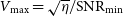 $V_\mathrm{max}=\sqrt{\eta}/\mathrm{SNR}_\mathrm{min}$
which bounds the top of the distribution (red dashed line).
$V_\mathrm{max}=\sqrt{\eta}/\mathrm{SNR}_\mathrm{min}$
which bounds the top of the distribution (red dashed line).

6.1.4.
$\eta$
-V parameters

It has become standard to consider both the reduced
 $\chi^2$
:
$\chi^2$
:
 \begin{equation} \eta = \frac{1}{N-1} \chi^2_\mathrm{lc}\end{equation}
(where there are
 $N-1$
degrees of freedom) and the modulation index V together in finding variables which would have high values of
$N-1$
degrees of freedom) and the modulation index V together in finding variables which would have high values of
 $\eta$
, V, or both (e.g. Swinbank et al. Reference Swinbank2015; Rowlinson et al. Reference Rowlinson2019).
$\eta$
, V, or both (e.g. Swinbank et al. Reference Swinbank2015; Rowlinson et al. Reference Rowlinson2019).
Both of these statistics are based on the second moments of the flux density (i.e. variance or standard deviation), and both are independent of data order. So they should convey some similar information. However, while correlated, the outliers in
 $\eta$
or V are not always the same. As discussed by Rowlinson et al. (Reference Rowlinson2019), sources with high
$\eta$
or V are not always the same. As discussed by Rowlinson et al. (Reference Rowlinson2019), sources with high
 $\eta$
usually are brighter, have some large flares or similar excursions from the mean, and have low uncertainties relative to the mean. Such lightcurves are statistically distinguishable from a constant value, although this relies on accurate calibration and error analysis at high signal-to-noise, which is not always reliable. In contrast, sources with high V typically have lower average flux densities.
$\eta$
usually are brighter, have some large flares or similar excursions from the mean, and have low uncertainties relative to the mean. Such lightcurves are statistically distinguishable from a constant value, although this relies on accurate calibration and error analysis at high signal-to-noise, which is not always reliable. In contrast, sources with high V typically have lower average flux densities.
This is illustrated in Figure 9, which consists entirely of simulated data with Gaussian noise and a range of signal-to-noise ratios (SNRs)Footnote
o
but no transients or variables beyond those expected from the noise realisations. As expected, at high V the data are dominated by low SNR sources that just happened to have slightly higher noise realisations. The trend with
 $\eta$
is harder to see, but at a constant V there is a trend toward higher
$\eta$
is harder to see, but at a constant V there is a trend toward higher
 $\eta$
at higher SNR. We also show the theoretical predictions for the marginal distributions. In the case of
$\eta$
at higher SNR. We also show the theoretical predictions for the marginal distributions. In the case of
 $\eta$
it is a scaled
$\eta$
it is a scaled
 $\chi^2$
distribution (as expected), which indeed resembles a log-normal distribution as discussed by Rowlinson et al. (Reference Rowlinson2019). For V the distribution is largely just the distribution of
$\chi^2$
distribution (as expected), which indeed resembles a log-normal distribution as discussed by Rowlinson et al. (Reference Rowlinson2019). For V the distribution is largely just the distribution of
 $1/\mathrm{SNR}$
, which will depend on the underlying flux density distribution: since in this simulation S has a power-law distribution and
$1/\mathrm{SNR}$
, which will depend on the underlying flux density distribution: since in this simulation S has a power-law distribution and
 $\mathrm{SNR}\propto S$
(constant noise), V also has a power-law distribution up to the maximum value but with an inverted index,
$\mathrm{SNR}\propto S$
(constant noise), V also has a power-law distribution up to the maximum value but with an inverted index,
 $N(\gt V)\propto V^{1.5}$
. This can change in other samples, though. Finally, we also see a cutoff at high V that depends on
$N(\gt V)\propto V^{1.5}$
. This can change in other samples, though. Finally, we also see a cutoff at high V that depends on
 $\eta$
as
$\eta$
as
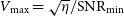 $V_\mathrm{ max}=\sqrt{\eta}/\mathrm{SNR}_\mathrm{min}$
: such cutoffs are observed in real data (e.g. Rowlinson et al. Reference Rowlinson2019; Murphy et al. Reference Murphy2021).
$V_\mathrm{ max}=\sqrt{\eta}/\mathrm{SNR}_\mathrm{min}$
: such cutoffs are observed in real data (e.g. Rowlinson et al. Reference Rowlinson2019; Murphy et al. Reference Murphy2021).
This demonstration serves several purposes. Firstly, the use of both
 $\eta$
and V, while common, is not necessarily optimal since they are related to each other as a function of SNR. A better second metric in addition to
$\eta$
and V, while common, is not necessarily optimal since they are related to each other as a function of SNR. A better second metric in addition to
 $\eta$
or V might be something optimised for detecting short-timescale variability such as the result of an outlier search or a matched filter, or some other metric that incorporates information about the order of the data. Secondly, the background distribution of
$\eta$
or V might be something optimised for detecting short-timescale variability such as the result of an outlier search or a matched filter, or some other metric that incorporates information about the order of the data. Secondly, the background distribution of
 $\eta$
should follow a
$\eta$
should follow a
 $\chi^2$
distribution, while that of V depends on the range of SNRs considered, and both can be used to determine thresholds for investigation.
$\chi^2$
distribution, while that of V depends on the range of SNRs considered, and both can be used to determine thresholds for investigation.
6.1.5. Other variability metrics
The metrics discussed in the previous section are related: they are both second-order statistics that depend on the degree of variability but ignore any shape/ordering of the lightcurve. Hence a number of other metrics or analyses have been used in different cases.
Perhaps the simplest is the temporal gradient
 $\nabla_F \equiv dS/dt$
used by Bell et al. (Reference Bell2019), who also divided the gradient by its uncertainty,
$\nabla_F \equiv dS/dt$
used by Bell et al. (Reference Bell2019), who also divided the gradient by its uncertainty,
 $\nabla_S \equiv \nabla_F/\sigma_F$
to identify statistically significant changes. They also found that higher-order polynomial changes were not needed to describe the data.
$\nabla_S \equiv \nabla_F/\sigma_F$
to identify statistically significant changes. They also found that higher-order polynomial changes were not needed to describe the data.
More general parameterisations use the autocorrelation function:
 \begin{equation} ACF(\tau) = \langle S(t+\tau)S(t)\rangle,\end{equation}
which is sometimes replaced by the autocovariance function (also ACF):
 \begin{equation} ACF(\tau) = \langle [S(t+\tau)-\overline{S}][S(t)-\overline{S}]\rangle,\end{equation}
where the means are subtracted before calculation. Both of these determine the ACF as a function of lag
 $\tau$
. The autocorrelation function can be used to study the timescale of variations (Rickett Reference Rickett1977), especially for diffractive scintillation in pulsars. A similar concept is the structure function:
$\tau$
. The autocorrelation function can be used to study the timescale of variations (Rickett Reference Rickett1977), especially for diffractive scintillation in pulsars. A similar concept is the structure function:
 \begin{equation} D(\tau) = \langle [F(t+\tau) - F(t)]^2 \rangle\end{equation}
for all measurements in some bin with lag
 $\tau$
, where F can be the raw flux density measurements (Hughes et al. Reference Hughes, Aller and Aller1992; Kumamoto et al. Reference Kumamoto2021), but also measurements with the mean subtracted and then normalised by the standard deviation (Gaensler & Hunstead Reference Gaensler and Hunstead2000), or just normalised by the mean (Rickett & Lyne Reference Rickett and Lyne1990; Kaspi & Stinebring Reference Kaspi and Stinebring1992; Lovell et al. Reference Lovell2008). This is commonly used to study variability in AGN (Hughes et al. Reference Hughes, Aller and Aller1992; Lovell et al. Reference Lovell2008; Gaensler & Hunstead Reference Gaensler and Hunstead2000) and pulsars (Rickett & Lyne Reference Rickett and Lyne1990; Kaspi & Stinebring Reference Kaspi and Stinebring1992; Kumamoto et al. Reference Kumamoto2021) which can be compared against the predictions for refractive scintillation (e.g. Hancock et al. Reference Hancock, Charlton, Macquart and Hurley-Walker2019). Using expectations for the behaviour of the structure function with lag, it can be used to give a better definition of the modulation index and its associated timescale (e.g. Kaspi & Stinebring Reference Kaspi and Stinebring1992). In both cases effort must be taken to do this correctly for irregularly-sampled data (Edelson & Krolik Reference Edelson and Krolik1988; Kreutzer et al. Reference Kreutzer, Gillen, Briegal and Queloz2023).
$\tau$
, where F can be the raw flux density measurements (Hughes et al. Reference Hughes, Aller and Aller1992; Kumamoto et al. Reference Kumamoto2021), but also measurements with the mean subtracted and then normalised by the standard deviation (Gaensler & Hunstead Reference Gaensler and Hunstead2000), or just normalised by the mean (Rickett & Lyne Reference Rickett and Lyne1990; Kaspi & Stinebring Reference Kaspi and Stinebring1992; Lovell et al. Reference Lovell2008). This is commonly used to study variability in AGN (Hughes et al. Reference Hughes, Aller and Aller1992; Lovell et al. Reference Lovell2008; Gaensler & Hunstead Reference Gaensler and Hunstead2000) and pulsars (Rickett & Lyne Reference Rickett and Lyne1990; Kaspi & Stinebring Reference Kaspi and Stinebring1992; Kumamoto et al. Reference Kumamoto2021) which can be compared against the predictions for refractive scintillation (e.g. Hancock et al. Reference Hancock, Charlton, Macquart and Hurley-Walker2019). Using expectations for the behaviour of the structure function with lag, it can be used to give a better definition of the modulation index and its associated timescale (e.g. Kaspi & Stinebring Reference Kaspi and Stinebring1992). In both cases effort must be taken to do this correctly for irregularly-sampled data (Edelson & Krolik Reference Edelson and Krolik1988; Kreutzer et al. Reference Kreutzer, Gillen, Briegal and Queloz2023).
These functions are also intrinsically related to the Fourier power spectrum and its extension for irregularly-sampled data, the Lomb-Scargle power spectrum (Scargle Reference Scargle1982, Reference Scargle1989). Such power spectra can be estimated directly when searching for explicitly periodic emission, such as from eclipsing pulsar systems (e.g. Zic et al. Reference Zic2024; Petrou et al. Reference Petrou2025). There are also many refinements to these broad techniques such as Gaussian processes (Aigrain & Foreman-Mackey Reference Aigrain and Foreman-Mackey2023), but in the cases of radio lightcurves with only a few tens of data-points for most examples, the differences between the techniques are small.
Furthermore, Fourier techniques can be seen as matched filters with sine/cosine kernel functions with unknown period. This can be explored further with more specific kernels that are appropriate to specific transient types. For example, Leung et al. (Reference Leung, Murphy, Lenc, Edwards, Ghirlanda, Kaplan, O’Brien and Wang2023) designed a matched filter around the expected shape of a GRB afterglow, especially orphan afterglows, parameterised as a power-law lightcurve with an optional break. Compared to selection via a standard techniques selecting sources compared to a constant model (effectively the
 $\chi^2_\mathrm{lc}$
in Equation 9), none of the five selected sources from that paper would have passed a more basic
$\chi^2_\mathrm{lc}$
in Equation 9), none of the five selected sources from that paper would have passed a more basic
 $3\sigma$
threshold due to their slow evolution. Such a strategy can of course be adopted for an arbitrary light-curve shape, such as a generic burst. All of these techniques, though, require richer data sets with at least tens (if not more) samples, which are only becoming common with the latest generation of surveys.
$3\sigma$
threshold due to their slow evolution. Such a strategy can of course be adopted for an arbitrary light-curve shape, such as a generic burst. All of these techniques, though, require richer data sets with at least tens (if not more) samples, which are only becoming common with the latest generation of surveys.
6.1.6. Burst detection
In time-domain surveys with small numbers of temporal samples (observing epochs or otherwise), there is in general no need for explicit burst detection beyond the variability analysis presented above. But as the number of samples grows, especially with short integrations from longer images (Section 5.1), the need for explicit burst detection grows.
Historically, there has not been a large focus on burst detection from radio images, largely due to the small number of samples available. This is in contrast to the significant literature in finding and classifying bursts in other domains such as FRBs (e.g. Rajwade & van Leeuwen Reference Rajwade and van Leeuwen2024) or XRBs and GRBs (e.g. Barthelmy et al. Reference Barthelmy2005; Meegan et al. Reference Meegan2009). Those cases are made further difficult by the need to examine large data-sets in real time – leading to efficient hardware implementations, machine learning classifiers, and distributed architectures – something which radio imaging surveys are only now starting to confront.
Beyond initial approaches using the metrics above or variants, there can be techniques that segment the data into ‘background’ and ‘burst’. At the simplest level, iterative sigma clipping (e.g. Leroy & Rousseeuw Reference Leroy and Rousseeuw1987) is often used for outlier excision (Vallisneri & van Haasteren Reference Vallisneri and van Haasteren2017), but can be used for outlier identification as well. More complex approaches can be taken to the same problem (e.g. Hogg, Bovy, & Lang Reference Hogg, Bovy and Lang2010) with robust statistical models that attempt to assign probabilities to each data point regarding whether it is part of the background or not. However, these approaches may be limited in that they consider each observation independently. If the burst duration is less than the sampling time that is fine, but if bursts can last longer then techniques which take into account the temporal relation between data points may be preferred.
The basic techniques used in those cases are typically variants of matched filtering (also see Section 5.2), which is also commonly used for FRB detection (after dedispersion). Typically a Gaussian or boxcar filter (if there is a priori knowledge that the burst shape should be different that could of course be used instead, or a more complex basis like wavelets if there are enough samples) of a given width is convolved with the data to identify bursts, and then this is repeated for a range of widths. And as with the outlier detection metrics above, a more formal Bayesian approach can be taken here too. For instance, Scargle et al. (Reference Scargle, Norris, Jackson and Chiang2013) offer an efficient algorithm that can identify segments of arbitrary length which differ from the background, and which can be applied to data arriving in real time and to data which have already been collected. This algorithm achieves similar sensitivity to the theoretical limit.
6.2. Populations and rates
In many previous papers, where transients were identified from 2-epoch searches in small numbers, often years after the fact (limiting followup possibilities), the results were presented as a limit or constraint on the rate (areal density) of transient sources (e.g. Bower & Saul Reference Bower and Saul2011; Croft et al. Reference Croft2010, Reference Croft, Bower, Keating, Law, Whysong, Williams and Wright2011; Stewart et al. Reference Stewart2016; Rowlinson et al. Reference Rowlinson2016; Bell et al. Reference Bell2011, Reference Bell, Huynh, Hancock, Murphy, Gaensler, Burlon, Trott and Bannister2015, Reference Bell2014; Bhandari et al. 2018; Mooley et al. Reference Mooley, Frail, Ofek, Miller, Kulkarni and Horesh2013); see Mooley et al. (Reference Mooley2016) for a nice compilation that has been recently updated.Footnote p This served to help develop expectations for improved surveys, as well as understand the discovery rate relative to the expected rates of various source populations (e.g. Metzger et al. Reference Metzger, Williams and Berger2015b ). This analysis particularly applied to synchrotron transients, which have very similar lightcurves.
However, the changes outlined in Section 4.5 have changed this practice. Firstly, using multi-epoch surveys makes the distinction between transients and variables less clear. Although some sources are clearly explosive in origin and hence intrinsically ‘transient’, many of the sources identified by earlier surveys are more clearly examples of variable sources when richer data sets are used (e.g. Murphy et al. Reference Murphy2021). This also means that lightcurve shape can influence the inferred transient rate explicitly, as described in detail by Carbone et al (Reference Carbone2016, Reference Carbone, van der Horst, Wijers and Rowlinson2017). Those works include more powerful but also more specific techniques to constrain the rates of individual source populations. These approaches rely on assumptions about the underlying source properties and distributions, as well as detailed knowledge of the observing strategy (similar to Feindt et al. Reference Feindt, Nordin, Rigault, Brinnel, Dhawan, Goobar and Kowalski2019). For a general review such as this, it is difficult to do a comprehensive analysis for a large set of previous surveys and sources. Secondly, faster identification has allowed much more reliable followup and classification (e.g. Law et al. Reference Law, Gaensler, Metzger, Ofek and Sironi2018b ; Anderson et al. Reference Anderson2020; Dong et al. Reference Dong2021; Dong & Hallinan Reference Dong and Hallinan2023). Thirdly, searches for shorter-duration events and polarised sources have allowed discovery of new classes of sources besides synchrotron transients (e.g. Hurley-Walker et al. Reference Hurley-Walker2022b , Reference Hurley-Walker2023; Caleb et al. Reference Caleb2024; Lee et al. Reference Lee2025; Wang et al. Reference Wang2021b , Reference Wang2025c ; Dong et al. Reference Dong2025b ). Finally, the latest generation of surveys (VLASS, VAST, LoTSS, MWA GPM) are still ongoing, with individual sources being published and final tallies of discoveries still to come. All of these make the continuation of overall rate projections less valuable. Rates are extremely valuable still for studying individual classes of objects (e.g. Beniamini et al. Reference Beniamini, Wadiasingh, Hare, Rajwade, Younes and van der Horst2023) but we do not focus on the ‘transient rate’.
These recent surveys have allowed us to start to characterise the overall populations of radio transients and variables for the first time. Figure 10 shows the number of each source type found in a selection of recent surveys. Most surveys found AGN/galaxies as the dominant class (except for Dobie et al. Reference Dobie2023 who deliberately excluded them), followed by radio stars and pulsars.
Source class distribution for the transient and variable sources found in a selection of recent image-domain surveys: Wang et al. (Reference Wang2023), who searched for minute-scale variability at frequencies near 1 GHz with ASKAP; Murphy et al. (Reference Murphy2021), who searched for longer-scale variability at 888 MHz with ASKAP; Dobie et al. (Reference Dobie2023), who searched for fast variability at 943 MHz with ASKAP; Rowlinson et al. (Reference Rowlinson2022), who searched for variability on timescales of weeks at 1.4 GHz with MeerKAT; Sarbadhicary et al. (Reference Sarbadhicary2021), who searched for longer-scale variability in deep images with the VLA at 1–2 GHz; and Chastain et al. (Reference Chastain2025), who searched for short-term variability with MeerKAT at 1.3 GHz. Most surveys show AGN & galaxies as the dominant class, except for Dobie et al. (Reference Dobie2023) who deliberately excluded them. Since each survey had very different fields-of-view and total numbers of epochs we do not present absolute numbers, but just relative populations, and even those will change for different surveys (e.g. stars and pulsars will be over-represented on shorter timescales).

We have looked at the potential discovery volume from different past/ongoing surveys (Figure 7) but more to show the overall progression with time, rather than to allow direct comparison. The proliferation of survey strategies probing different timescales with different techniques has made such comparisons increasingly hard (e.g. Rowlinson et al. Reference Rowlinson2016). In the following section, we look toward future facilities (for which the details of potential surveys are still unclear) to see broadly where they might excel, but we still do not give detailed projections for yields. This is best left to in-depth analyses that examine specific source classes.
Specifications for future radio telescopes.

 $^\mathrm{a}$
Multiple configurations trading bandwidth between HBA and LBA arrays and multiple beams are possible. Most specifications are for the full EU array.
$^\mathrm{a}$
Multiple configurations trading bandwidth between HBA and LBA arrays and multiple beams are possible. Most specifications are for the full EU array.
 $^\mathrm{b}$
Based on https://www.astron.nl/telescopes/square-kilometre-array/, Dewdney et al. (Reference Dewdney2022), and https://sensitivity-calculator.skao.int/mid. Most specifications are for Band 2, containing 1.4 GHz. Sensitivity and resolution can be changed with different weighting schemes.
$^\mathrm{b}$
Based on https://www.astron.nl/telescopes/square-kilometre-array/, Dewdney et al. (Reference Dewdney2022), and https://sensitivity-calculator.skao.int/mid. Most specifications are for Band 2, containing 1.4 GHz. Sensitivity and resolution can be changed with different weighting schemes.
 $^\mathrm{c}$
Based on https://ngect.nrao.edu. Most specifications are for the ‘main’ (core plus spiral out to 1000 km) array and for Band 1 (centred at 2.4 GHz).
$^\mathrm{c}$
Based on https://ngect.nrao.edu. Most specifications are for the ‘main’ (core plus spiral out to 1000 km) array and for Band 1 (centred at 2.4 GHz).
 $^{\mathrm{d}}$
At 1.4 GHz.
$^{\mathrm{d}}$
At 1.4 GHz.
 $^\mathrm{e}$
Defined as
$^\mathrm{e}$
Defined as
 $\Omega A_\mathrm{eff}^2/T_\mathrm{sys}^2$
.
$\Omega A_\mathrm{eff}^2/T_\mathrm{sys}^2$
.
7. Previewing future transient surveys
The substantial amount of effort that has been put into conducting image domain radio transient surveys over the past 15 years has resulted in significant steps forward in our understanding of individual radio transient source types, of the overall populations, and of the advantages and limitations of various approaches to transient identification and classification.
It is critical that we draw on this experience to optimise the scientific benefit of the surveys that will be possible on upcoming radio telescopes. In this section we outline the specifications of three major future instruments, summarise some of the other planned facilities, and reflect on lessons learned from current transient surveys.
We summarise the basic properties of the telescopes in Table 6. Note that this does not contain details of prospective surveys. Some of the facilities will be primarily survey-driven, while others will be used more for PI-led science including transient followup. So focusing on the ‘survey speed’ may not be the most relevant metric. Nonetheless, we do present a survey speed calculated for each facility as:
 \begin{equation} \mathrm{SS} \equiv \Omega_\mathrm{inst} \frac{A_\mathrm{eff}^2}{T_\mathrm{sys}^2}.\end{equation}
Unlike in Section 4.2.1,
 $\Omega_\mathrm{inst}$
here is the instantaneous telescope field-of-view, since we are discussing telescopes and not surveys. In principle this should actually be an integral of the sensitivity over solid angle (e.g., Hotan et al. Reference Hotan2021), but such information is not always available. In some uses survey speed can also include a bandwidth factor (so that it more directly reflects the time needed to achieve a given flux density limit over a given area), but we do not do that here.
$\Omega_\mathrm{inst}$
here is the instantaneous telescope field-of-view, since we are discussing telescopes and not surveys. In principle this should actually be an integral of the sensitivity over solid angle (e.g., Hotan et al. Reference Hotan2021), but such information is not always available. In some uses survey speed can also include a bandwidth factor (so that it more directly reflects the time needed to achieve a given flux density limit over a given area), but we do not do that here.
This survey speed is intended to be proportional to the expected speed it would take to survey the sky down to a constant limiting flux density (and higher is better), although it does ignore some elements like changing bandwidth between telescopes or other sources of noise like confusion (compared to Equation 5 which uses the delivered noise). Note that we can relate the survey speed to the system equivalent flux density:
 \begin{equation} \mathrm{SEFD} \equiv \frac{2 k_B T_\mathrm{sys}}{A_\mathrm{eff}}\end{equation}
via
 \begin{equation} \mathrm{SS} = \Omega_\mathrm{inst} \frac{4k_B^2}{\mathrm{SEFD}^2}\end{equation}
and the continuum sensitivity
 \begin{equation} \sigma = \frac{\mathrm{SEFD}}{\sqrt{N_p \Delta t \Delta \nu}}\end{equation}
with
 $N_p=2$
the number of polarisations,
$N_p=2$
the number of polarisations,
 $\Delta t$
the integration time, and
$\Delta t$
the integration time, and
 $\Delta \nu$
the bandwidth (and this ignores any loss of sensitivity from uv tapering or weighting). So we also have
$\Delta \nu$
the bandwidth (and this ignores any loss of sensitivity from uv tapering or weighting). So we also have
 \begin{equation} \mathrm{SS} = \Omega_\mathrm{inst} \frac{4 k_B^2}{N_p \Delta t \Delta \nu \sigma^2}\end{equation}
In addition, comparisons between telescopes operating at very different frequencies are complicated by the changing sensitivities and bandwidths, together with expected source characteristics. Instead of an explicit spectral correction like in Equation 5 we separate the high (
 $\sim 1.4\,$
GHz) and low (
$\sim 1.4\,$
GHz) and low (
 $\lesssim 200\,$
MHz) facilities (especially as the contribution from Galactic synchrotron emission in the latter can be highly significant and highly variable with position).
$\lesssim 200\,$
MHz) facilities (especially as the contribution from Galactic synchrotron emission in the latter can be highly significant and highly variable with position).
In Figure 11 we plot the capabilities of the future facilities from Table 6 (which we discuss more below) along with current-generation facilities. We include both the survey speed, relevant for wide-field discovery, as well as the sensitivity (inverse of the SEFD), which is relevant for pointed followup. It is clear that the future facilities will have big improvements in both metrics, although the survey speed improvements will be most significant, and overall the boost at lower frequencies with the SKA-Low will be more significant than at higher frequencies.
Sensitivity of planned future radio facilities. We show the survey speed (Equation 18) in the top panel and the sensitivity (
 $A_\mathrm{eff}/T_\mathrm{sys}$
, from Equation 19) in the bottom panel as a function of frequency. Current facilities are shown with thinner lines, while future facilities are with thicker lines. The data are a mix of detailed calculations and simplistic projection (e.g. ignoring effective area changes within a frequency band). Data sources for future facilities are: DSA-2000 from G. Hallinan (pers. comm.), ngVLA from https://github.com/dlakaplan/, SKA1-low from http://skalowsensitivitybackup-env.eba-daehsrjt.ap-southeast-2.elasticbeanstalk.com, and SKA1-mid from https://gitlab.com/ska-telescope/ost/ska-ost-senscalc. Data sources for current facilities are: MeerKAT from https://gitlab.com/ska-telescope/ost/ska-ost-senscalc, upgraded GMRT (uGMRT) from Gupta et al. (Reference Gupta2017), VLA from https://science.nrao.edu/facilities/vla/docs/manuals/oss/performance, ASKAP from Hotan et al. (Reference Hotan2021) and E. Lenc (pers. comm.), LOFAR from van Haarlem et al. (Reference van Haarlem2013) for the Dutch array but with double the number of LBA antennas per station, and MWA from Ung (Reference Ung2019) via https://github.com/ysimonov/MWA-Sensitivity. Facilities at
$A_\mathrm{eff}/T_\mathrm{sys}$
, from Equation 19) in the bottom panel as a function of frequency. Current facilities are shown with thinner lines, while future facilities are with thicker lines. The data are a mix of detailed calculations and simplistic projection (e.g. ignoring effective area changes within a frequency band). Data sources for future facilities are: DSA-2000 from G. Hallinan (pers. comm.), ngVLA from https://github.com/dlakaplan/, SKA1-low from http://skalowsensitivitybackup-env.eba-daehsrjt.ap-southeast-2.elasticbeanstalk.com, and SKA1-mid from https://gitlab.com/ska-telescope/ost/ska-ost-senscalc. Data sources for current facilities are: MeerKAT from https://gitlab.com/ska-telescope/ost/ska-ost-senscalc, upgraded GMRT (uGMRT) from Gupta et al. (Reference Gupta2017), VLA from https://science.nrao.edu/facilities/vla/docs/manuals/oss/performance, ASKAP from Hotan et al. (Reference Hotan2021) and E. Lenc (pers. comm.), LOFAR from van Haarlem et al. (Reference van Haarlem2013) for the Dutch array but with double the number of LBA antennas per station, and MWA from Ung (Reference Ung2019) via https://github.com/ysimonov/MWA-Sensitivity. Facilities at
 $\lt300\,$
MHz include contributions from the sky temperature, although we use a pointing location away from the Galactic plane.
$\lt300\,$
MHz include contributions from the sky temperature, although we use a pointing location away from the Galactic plane.

7.1. The SKA Observatory
The SKA Observatory (SKAO) consists of two telescopes (SKA-Low and SKA-Mid), currently under construction.Footnote q SKA-Low will consist of 512 low frequency aperture array stations, spread over an area 80 km in diameter, located in Western Australia. Each station will have 256 wire antennas in a 38-m diameter area. It will observe in the frequency range 50–350 MHz. SKA-Mid will consist of 197 mid frequency dishes (64 from the existing MeerKAT array) spread over an area 180 km in diameter. It will be located in the Karoo region of South Africa. The telescope will operate in 6 frequency bands (3 initially) ranging from 350 MHz to 15.4 GHz. Full details and technical specifications of the telescopes are given in the Design Baseline Description and the SKAO Staged Delivery, Array Assemblies And Layouts documents and summarised in Table 6.
The SKAO telescopes are being constructed in stages, as outlined in the SKAO construction timeline.Footnote
r
A key milestone will be the completion of the AA
 $^*$
arrays, which will consist of 307 SKA-Low stations and 144 SKA-Mid dishes. These arrays are expected to be completed in 2029 and 2031, respectively, with the specifications summarised in Table 6.
$^*$
arrays, which will consist of 307 SKA-Low stations and 144 SKA-Mid dishes. These arrays are expected to be completed in 2029 and 2031, respectively, with the specifications summarised in Table 6.
The science case for the SKAO telescopes has been outlined in two paper collections. Firstly, in ‘Science with the Square Kilometre Array’ (Carilli & Rawlings Reference Carilli and Rawlings2004) and then, a decade later, in ‘Advancing Astrophysics with the Square Kilometre Array’ (Braun et al. Reference Braun, Bourke, Green, Keane and Wagg2015). A new science book, stemming from the 2025 SKAO General Science Meeting, ‘A new era in astrophysics: Preparing for early science with the SKAO’ is currently in preparation.
The exact operating model of the SKAO telescopes (including how time is allocated, and potential survey design) is yet to be determined. However, the current plan is that PI-led science would start in 2030 on AA
 $^*$
and larger observing programs led by the Key Science Projects would start several years later.
$^*$
and larger observing programs led by the Key Science Projects would start several years later.
7.2. DSA-2000
The DSA-2000 telescope is a planned instrument that, as originally scoped, will consist of
 $2\,000 \times 5$
-m dishes spanning an area of 19 km
$2\,000 \times 5$
-m dishes spanning an area of 19 km
 $\times$
15 km in Nevada, USA (Hallinan et al. Reference Hallinan2019). However, the array specification has changed to
$\times$
15 km in Nevada, USA (Hallinan et al. Reference Hallinan2019). However, the array specification has changed to
 $1\,650 \times 6.15$
-m (along with a new name, still to be determined), which will have a similar survey speed but a better point-source sensitivity (G. Hallinan, pers. comm.). The telescope will operate at radio frequencies of 700 MHz–2 GHz. The baseline reference design specifications are summarised in Table 6. The aim is to survey the sky repeatedly with a logarithmic cadence, with more of a focus on the Galactic plane.
$1\,650 \times 6.15$
-m (along with a new name, still to be determined), which will have a similar survey speed but a better point-source sensitivity (G. Hallinan, pers. comm.). The telescope will operate at radio frequencies of 700 MHz–2 GHz. The baseline reference design specifications are summarised in Table 6. The aim is to survey the sky repeatedly with a logarithmic cadence, with more of a focus on the Galactic plane.
The science case for DSA-2000 has been outlined in the Community Science Book.Footnote s There are four main science areas, two of which are directly relevant to this review: ‘the dynamic radio sky’ and ‘ multi-messenger astronomy’. Unlike the SKAO and ngVLA, there are no receivers to switch, so the DSA-2000 is planning on surveying the sky for its main science goals (with some time devoted to followup of multi-messenger transients). This, combined with the small element diameter and consequent large field-of-view, gives DSA-2000 a considerable advantage in survey speed compared to the other facilities at the same frequency.
7.3. The next-generation VLA
The next-generation Very Large Array (ngVLA; Murphy Reference Murphy2018) is a planned instrument that will consist of a Main array of
 $214\times 18\,$
m off-axis parabolic antennas distributed across the USA and Mexico, out to baselines of 1 000 km, plus another
$214\times 18\,$
m off-axis parabolic antennas distributed across the USA and Mexico, out to baselines of 1 000 km, plus another
 $30\times 18\,$
m dishes on continental baselines (out to 9 000 km) in the Long Baseline Array (LBA) and
$30\times 18\,$
m dishes on continental baselines (out to 9 000 km) in the Long Baseline Array (LBA) and
 $19\times 6\,$
m dishes in the Short Baseline Array for diffuse sources (which is of less interest for transient science). The array will operate in a frequency range from 1 to 116 GHz, with maximum bandwidth 20 GHz.
$19\times 6\,$
m dishes in the Short Baseline Array for diffuse sources (which is of less interest for transient science). The array will operate in a frequency range from 1 to 116 GHz, with maximum bandwidth 20 GHz.
In contrast to the SKAO and DSA-2000, the ngVLA is designed to be primarily a PI-driven instrument. It has 5 key science drivers, the most relevant to this review being: ‘Understanding the Formation and Evolution of Stellar and Supermassive Black Holes in the Era of Multi-Messenger Astronomy’. For the most part it is not planned that there will be large-scale surveys with the ngVLA, but it will certainly participate in dedicated time-domain followup studies, and the capabilities of the LBA for astrometry and precision measurements enable new science compared to what SKA and DSA-2000 offer on their own (e.g. Section 5.6).
7.4. LOFAR 2.0
The LOw-Frequency ARray (LOFAR; van Haarlem et al. Reference van Haarlem2013) is a network of 24 Core stations located near Dwingeloo in the Netherlands, 14 Remote stations distributed across the Netherlands and 14 larger International stations distributed over Europe. Each station consists of low band antennas (LBAs) that operate at 10–90 MHz and high band antennas (HBAs) that operate at 110–240 MHz.
LOFAR 2.0Footnote t is a major upgrade to the LOFAR telescope. Two new stations will be added. New low-noise amplifiers will be added to all antennas (Wang, Norden, & Donker Reference Wang, Norden and Donker2025a ), and processing improvements will allow simultaneous use of both LBAs and HBAs, or using two beams for each HBA station. There are also improvements in the clock distribution and central processing facility used for calibration and imaging, as well as a 24/7 transient buffer for imaging and localisation. The net result will be a more powerful and flexible system capable of optimising its operation for many different transient cases (timescales, sensitivities, etc), as well as general improvements in image fidelity and processing (enabling faster followup with better localisation).
The science case is outlined in the LOFAR 2.0 White Paper.Footnote u Transient science (including supernova, gamma-ray bursts, stellar activity and exploring the unknown), forms a major part of the science case.
7.5. All-sky radio transient monitors
To maximise the chance of detecting very rare, very bright events (e.g. fast radio bursts, long period transients, extreme stellar bursts, or coherent signals from neutron star mergers) it is desirable to maximise the time on sky. These can be achieved with existing and proposed facilities that can continuously monitor large fractions of the sky (e.g. Prasad et al. Reference Prasad2016; Bochenek et al. Reference Bochenek, McKenna, Belov, Kocz, Kulkarni, Lamb, Ravi and Woody2020a ; Sokolowski et al. Reference Sokolowski2021; Connor et al. Reference Connor2021; Lin et al. Reference Lin2022; Luo et al. Reference Luo2024; Kosogorov et al. Reference Kosogorov2025), which are being developed with increasing sensitivity and other capabilities. This strategy achieved notable success in detecting a FRB-like burst from a Galactic magnetar (Bochenek et al. Reference Bochenek, Ravi, Belov, Hallinan, Kocz, Kulkarni and McKenna2020b ), which served to motivate future experiments.
All-sky monitors have typically been designed to detect ‘fast’ transients, using multiple receivers or digital beamforming techniques rather than imaging. This leads to good performance for short-duration signals, especially those that have detectable dispersion across the band (helping with interference rejection), but means they have reduced sensitivity to longer-duration signals due to fluctuations in the receiver electronics. Nonetheless, there is overlap in the type of sources these systems can detect and those discussed in this review, such as the discovery of a LPT with period of 14 min by the CHIME FRB system (Dong et al. Reference Dong2025a , although note that the same source was independently detected through LOFAR imaging by Bloot et al. Reference Bloot2025). This discovery was helped by the relatively short pulse period and narrow duty cycle, such that individual pulses were short enough to be detected by the FRB system. Future explorations of the overlap between all-sky beamformed searches and more targeted imaging searches will help map out the underlying distribution of periods and fluences from sources like these.
8. Summary and outlook
Time domain studies have been important since the dawn of radio astronomy, and give us insight into physical phenomena that span orders of magnitude in luminosity (from stars in our local neighbourhood through to distant gamma-ray bursts); in timescale (from nanosecond pulses through to afterglows that evolve over years); and in physical properties (from highly dense, magnetised compact objects to scintillation caused by interstellar plasma). These regimes are often inaccessible via other observations and have led to numerous breakthroughs.
The field of image-domain transients has evolved from targeted studies of individual objects, to serendipitous coverage by generic surveys, through to custom designed large scale surveys. In the current decade (the 2020s), the plans mapped out many years ago have started to come to fruition, with a suite of telescopes reaching the sensitivity, resolution, and survey speed required to detect a wide range of radio transients at megahertz and gigahertz radio frequencies.
Some of the scientific highlights of the past decade (from both targeted and untargeted observations) include (with tentative results in italics):
-
• Detection of an extreme scattering event in real time (Bannister et al. Reference Bannister, Stevens, Tuntsov, Walker, Johnston, Reynolds and Bignall2016);
-
• Identification of persistent radio sources associated with Fast Radio Bursts (Chatterjee et al. Reference Chatterjee2017);
-
• Radio detection and monitoring of the afterglow from GW170817 (Hallinan et al. Reference Hallinan2017);
-
• Detection of a possible gamma-ray burst orphan afterglow ( Law et al. Reference Law, Gaensler, Metzger, Ofek and Sironi2018b ; Mooley et al. Reference Mooley2022 );
-
• Discovery of fast blue optical transients (FBOTs; Ho et al. Reference Ho2019);
-
• Tentative signs of radio emission from star-planet interactions ( Vedantham et al. Reference Vedantham2020 ).
-
• Detection of delayed radio flares from a tidal disruption event (Horesh et al. Reference Horesh, Cenko and Arcavi2021a );
-
• Precision measurement of the distance to and mass of the black hole X-ray binary Cygnus X-1 (Miller-Jones et al. Reference Miller-Jones2021);
-
• Detection of merger-triggered core collapse supernova (Dong et al. Reference Dong2021);
-
• Discovery of long period transients (Hurley-Walker et al. Reference Hurley-Walker2022b ; Caleb et al. Reference Caleb2022);
-
• First detection of radio emission from Type Ia supernova (Kool et al. Reference Kool2023);
-
• Substantial expansion of the known radio star population (Driessen et al. Reference Driessen2024);
-
• Identification of Type II radio burst from an M dwarf, suggestive of a coronal mass ejection (Callingham et al. Reference Callingham2025).
Many of these discoveries are only the first in their class (e.g. long period transients and fast blue optical transients), and have already been supplemented by further discoveries. Future surveys will continue to detect more examples, allowing us to understand the full underlying populations.
The diversity of these results show that we are long past the point of exploring the radio transient sky in a way that is uninformed by the properties of the underlying populations. While early surveys emphasised searching in ways that were independent of the time domain properties of the potential populations, we can now characterise the populations on very different timescales (contrast long period transients, with periods of seconds to hours; with gamma-ray bursts that evolve over months). Rather than counting the number of ‘transients’, we can instead study multiple classes.
Much of the planning over the past few decades has been framed in the context of preparation for SKAO-era radio transient surveys. With this in mind, we end with some reflections on lessons learned from the pathfinder and precursor surveys that we hope feed into the plans for upcoming surveys with the telescopes discussed in Section 7. Some of the things we think will be important are:
-
• Real-time imaging and transient detection: No major radio transient imaging survey so far has had the capability to detect transients in real time (unlike FRB surveys). This will be critical in opening up shorter timescales (by enabling rapid follow-up or more complex analysis), which are currently proving very productive in finding new classes of radio transients, and in enabling rapid follow-up of new detections.
-
• Commensal transient surveys: Serendipity is an important part of transient astronomy. To discover rare objects, it is important to maximise the time on sky. Hence continuing to have full commensal access to other large surveys, with dedicated rapid processing, for the purpose of transient detection is critical, and helps maximise the scientific output of our telescopes. Of course data processing in the era of massive datasets is not ‘free’, but the benefits of commensal transient surveys are likely to make this relatively minimal extra cost worthwhile.
-
• Custom-designed transient surveys: It is important to state that commensal observing is not enough to reveal and study populations of radio transients. We have now begun to characterise the time domain, spectral, and polarisation properties of a range of source classes. To maximise the chance of detection of the most interesting sources, custom-designed surveys that consider the time domain properties of specific populations are required.
-
• Radio follow-up capability: Large-scale widefield surveys are key to discovering rare events. However, understanding them often requires detailed radio monitoring across a range of frequencies. For example, to establish the spectral evolution of synchrotron sources, or establish periodic behaviour in stellar objects. Hence it is critical in the SKAO era that we maintain access to facilities that can be used for this follow-up, including VLBI.
-
• Multiwavelength coverage: Multiwavelength (optical, near-infrared, X-ray, gamma-ray) survey data is vital for assessing the nature of new discoveries. In general this does not have to be contemporaneous, although this is beneficial for some scientific goals. For example, stellar flares show significant structure within an event, so modelling requires multi-wavelength data, but triggering is impractical. For synchrotron transients, optical/IR data is required to identify a host galaxy, and archival high-energy data can be vital to determining whether it is a novel event like an orphan afterglow.
-
• Automatic classification of radio transients: Now we are detecting significant numbers of radio transients in untargeted surveys, it is important to have automatic methods for removing poor quality data, and for classifying transients and identifying the most interesting outliers. There are well-established approaches in optical transient surveys that are in relative infancy in radio. These should be developed and refined.
In addition, the capabilities identified in Section 4.5 are important considerations for future surveys.
Enormous progress has been made in the field of radio transient surveys in the past decades. The surveys (and targeted monitoring) conducted to date have been fruitful, and in some cases revealed new populations of objects. However, there are still many unanswered questions that we will be able to address when the telescopes currently under development come online. With such a substantial investment of time and resources, it is important we incorporate the lessons learned from our existing experience as we head into this new era of radio transients.
Acknowledgements
Thank you to the anonymous reviewer whose comments were very helpful in improving this manuscript, and to the editor, Minh Huynh, for advice and assistance throughout the publication process.
Huge thanks to Ron Ekers, Elaine Sadler, Dougal Dobie and Iris de Ruiter for feedback on parts of our draft manuscript. In preparing this review we drew on the very useful compilation of radio transient surveys and rates by Kunal Mooley. Thanks to Kunal (and Deepika Yadav) for updating their online table in time for this review. Thank you to Laura Driessen for permission to adapt the colour-magnitude diagram in Figure 5. Romy Pearse created the lightcurve sketches in Figure 8. Thank you also to Ashna Gulati for help preparing Figures 4 and 8. Finally, thanks to Liroy Lourenço for his help with references and the formatting of this manuscript. Of course any remaining errors in the text are our own.
We had useful interactions and discussions with many people in the preparation of this review. Particular thanks to Gemma Anderson, Shari Breen, Manisha Caleb, Fernando Camilo, Lauren Carter, Shami Chatterjee, Barnali Das, Paul Demorest, Iris de Ruiter, Dougal Dobie, Laura Driessen, Ashna Gulati, Gregg Hallinan, Natasha Hurley-Walker, Scott Hyman, Francois Kapp, Emil Lenc, Walter Max-Moerbeck, Eric Murphy, Joshua Pritchard, Kovi Rose, Antonia Rowlinson, Sarrvesh Sridhar, Randall Wayth, Michael Wheatland and Andrew Zic.
This research has made use of the Astrophysics Data System, funded by NASA under Cooperative Agreement 80NSSC21M00561. In conducting this review, generative AI tools (ChatGPT-4) were used to help search for relevant papers in the literature. No information or text directly from generative AI was used in the preparation of this manuscript.
This research was supported by the Australian Research Council Centre of Excellence for Gravitational Wave Discovery (OzGrav), project number CE230100016, and by National Science Foundation grant AST-2511757.


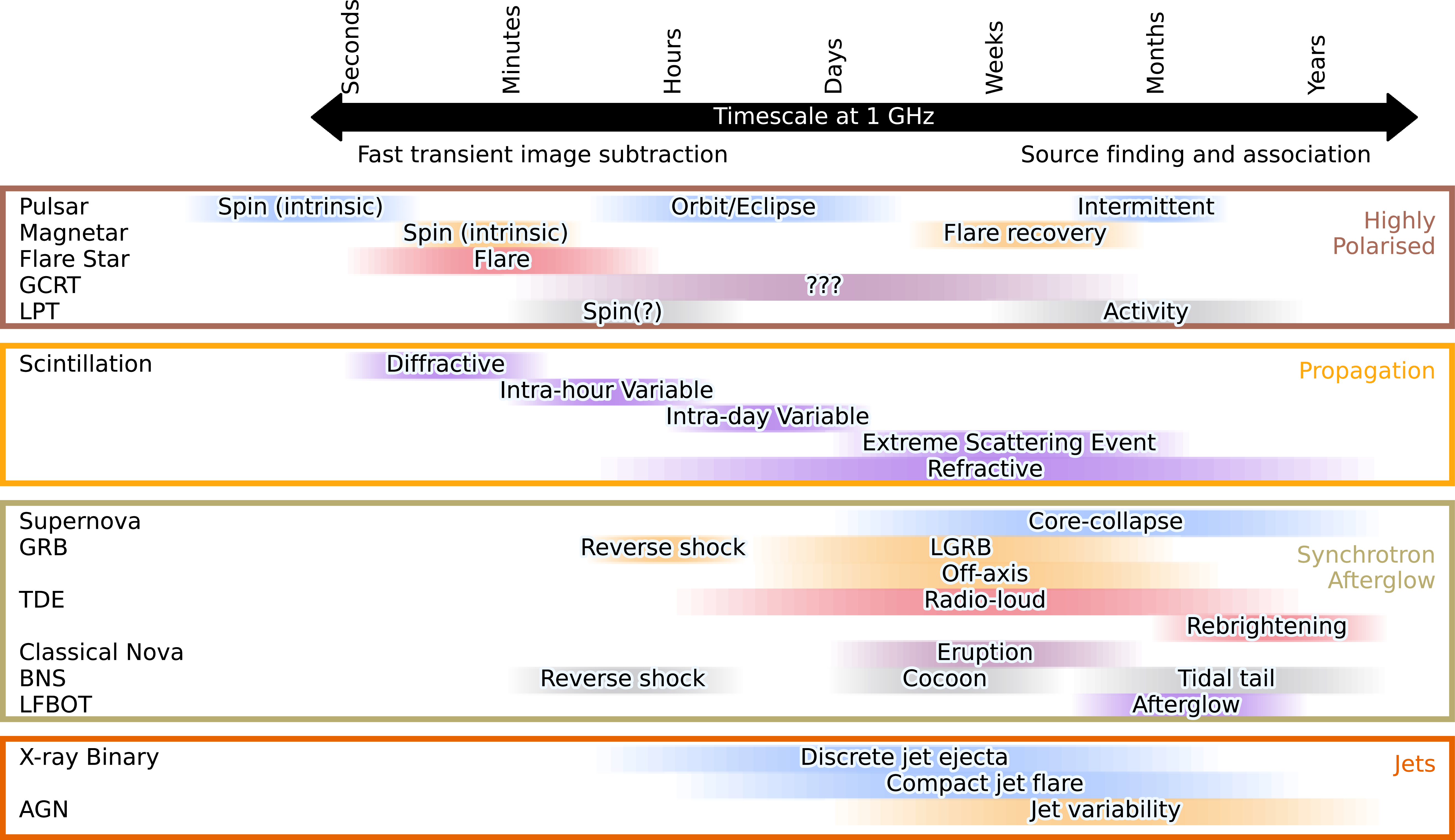


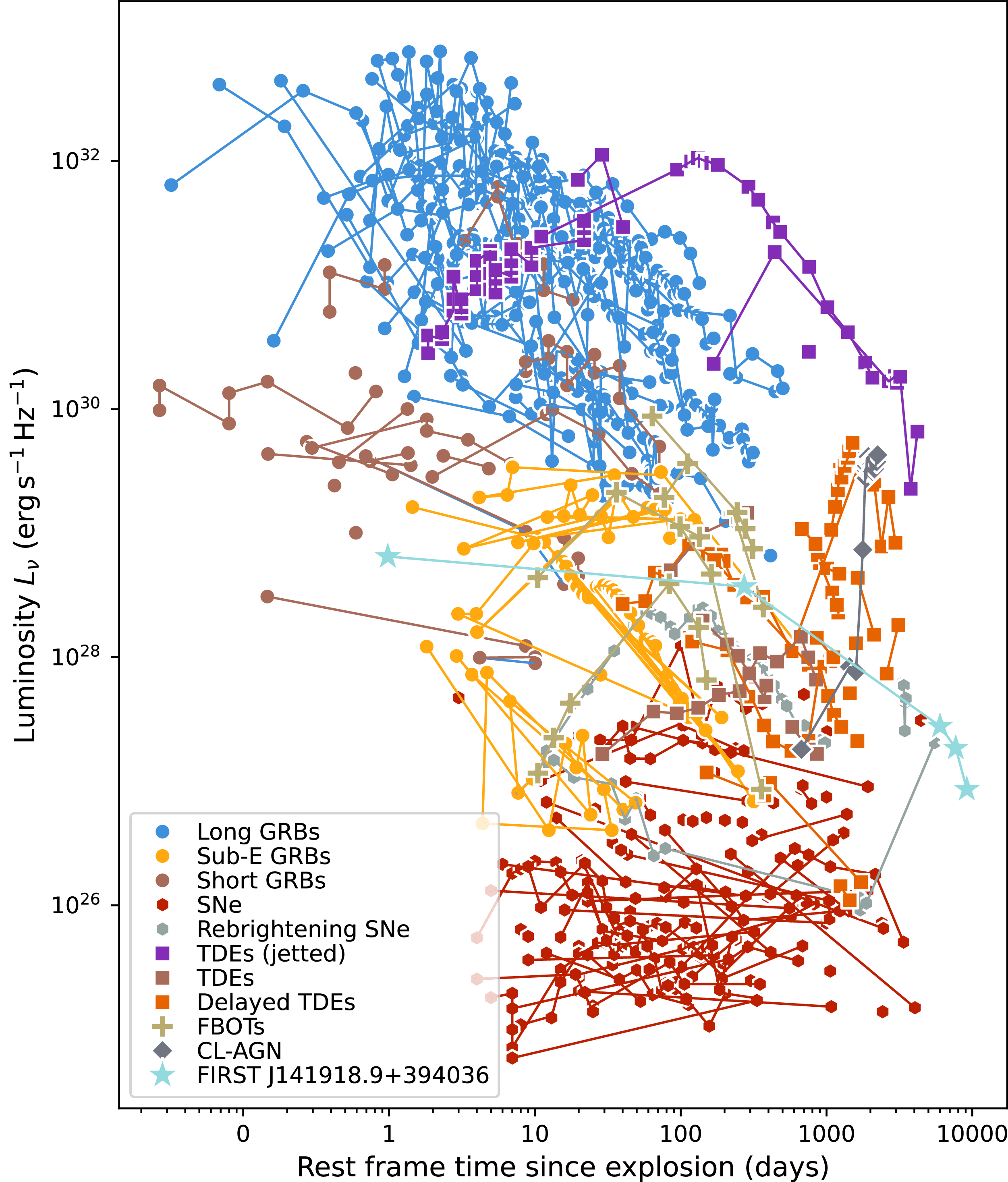
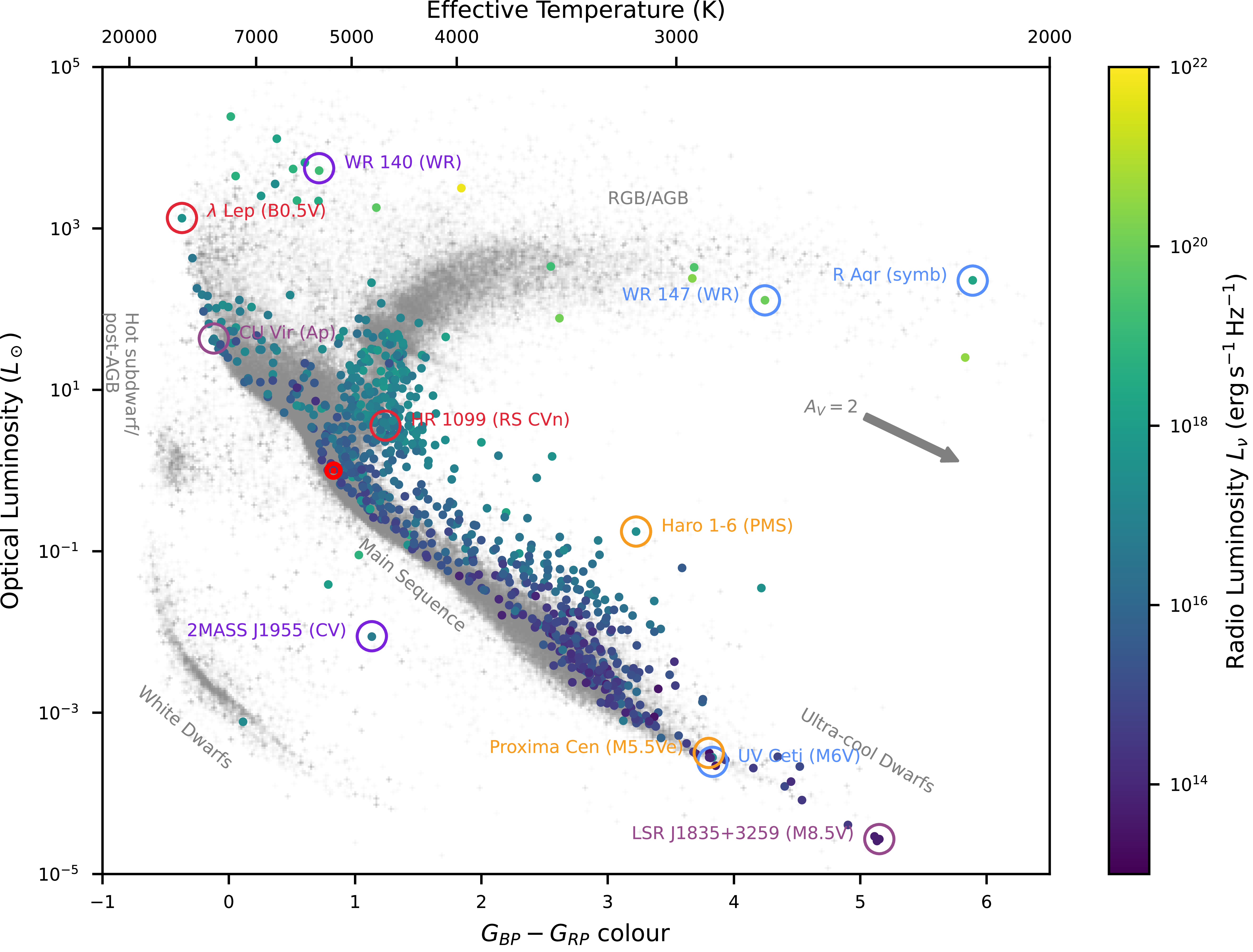


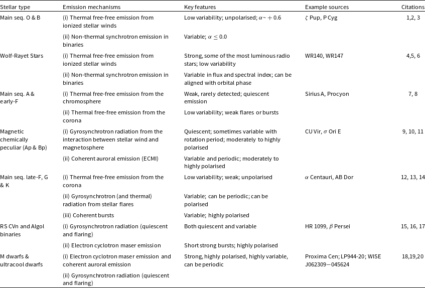
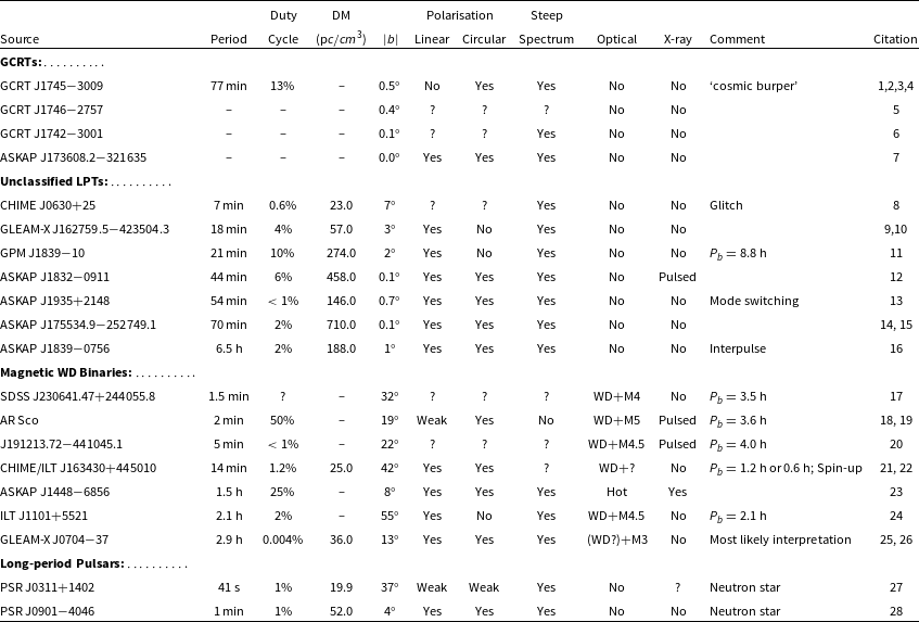
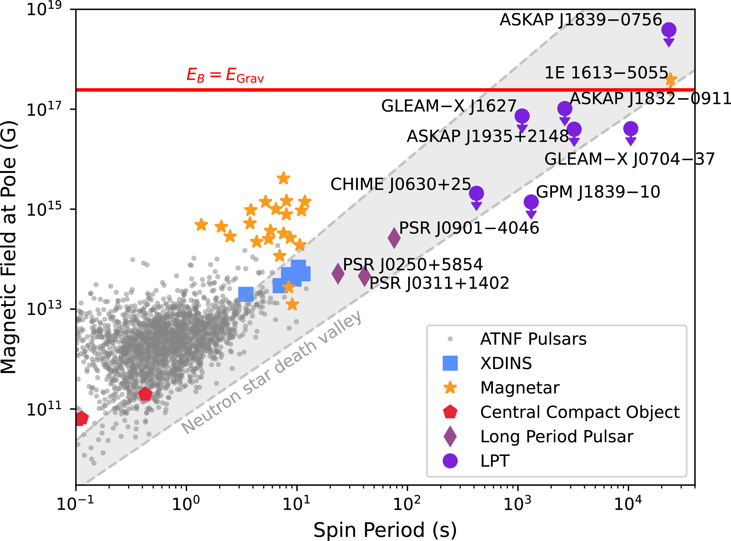


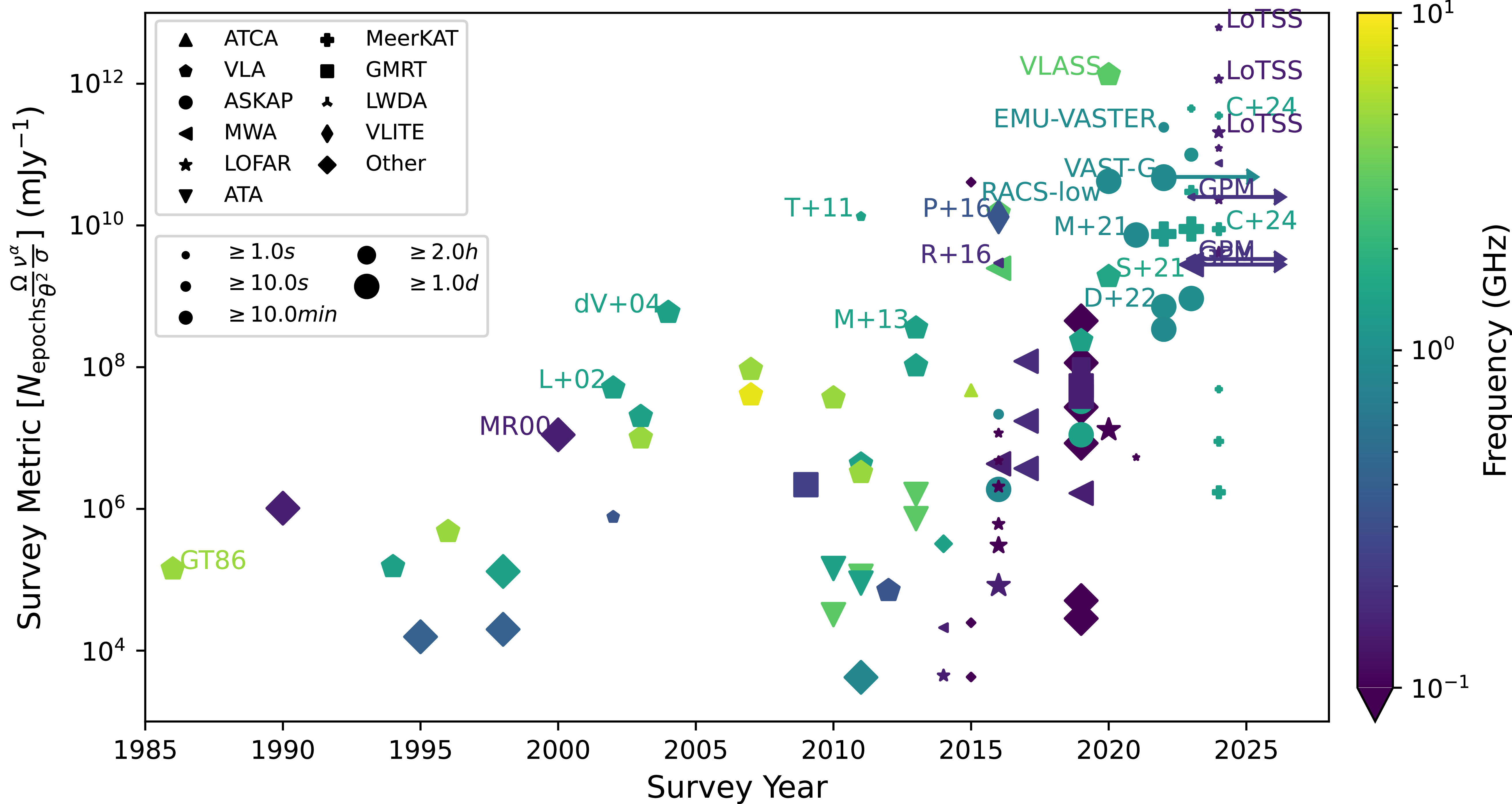
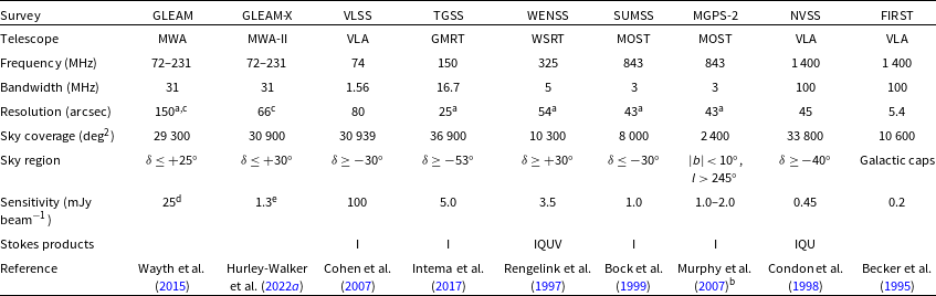
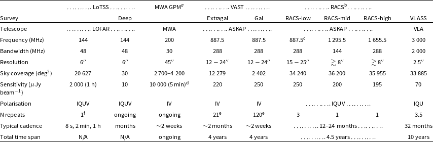
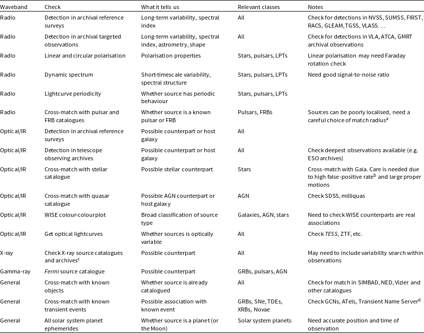
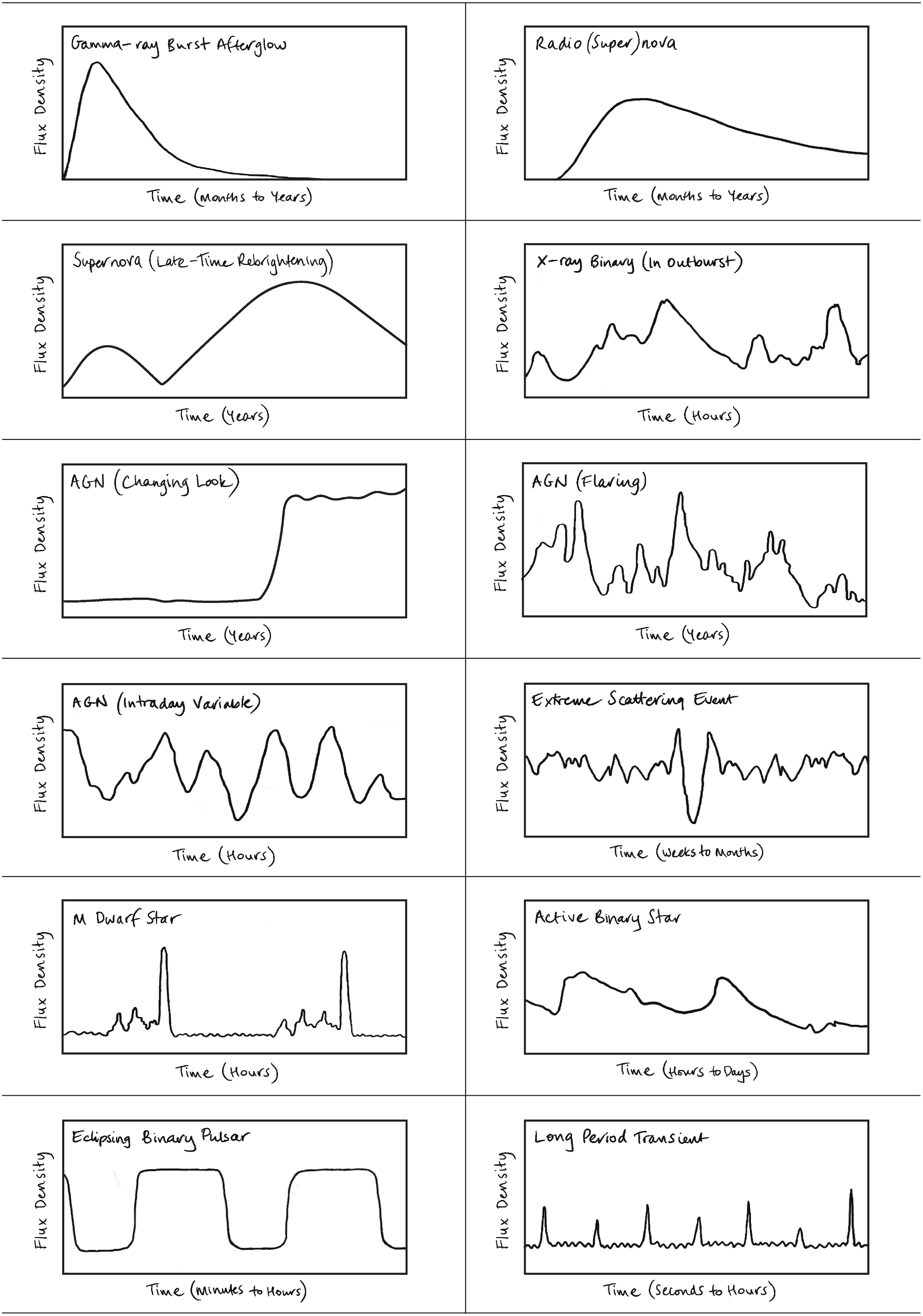
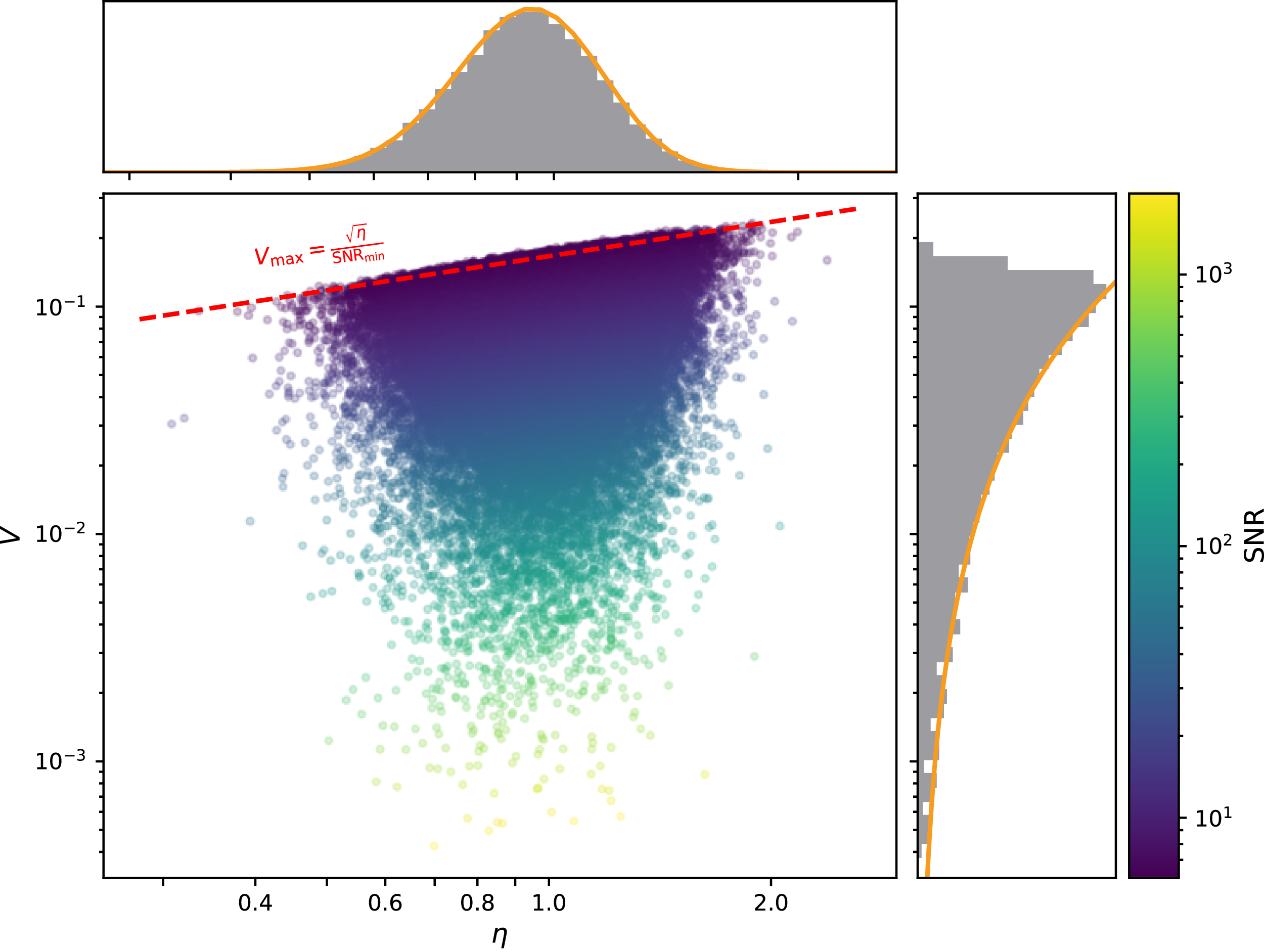


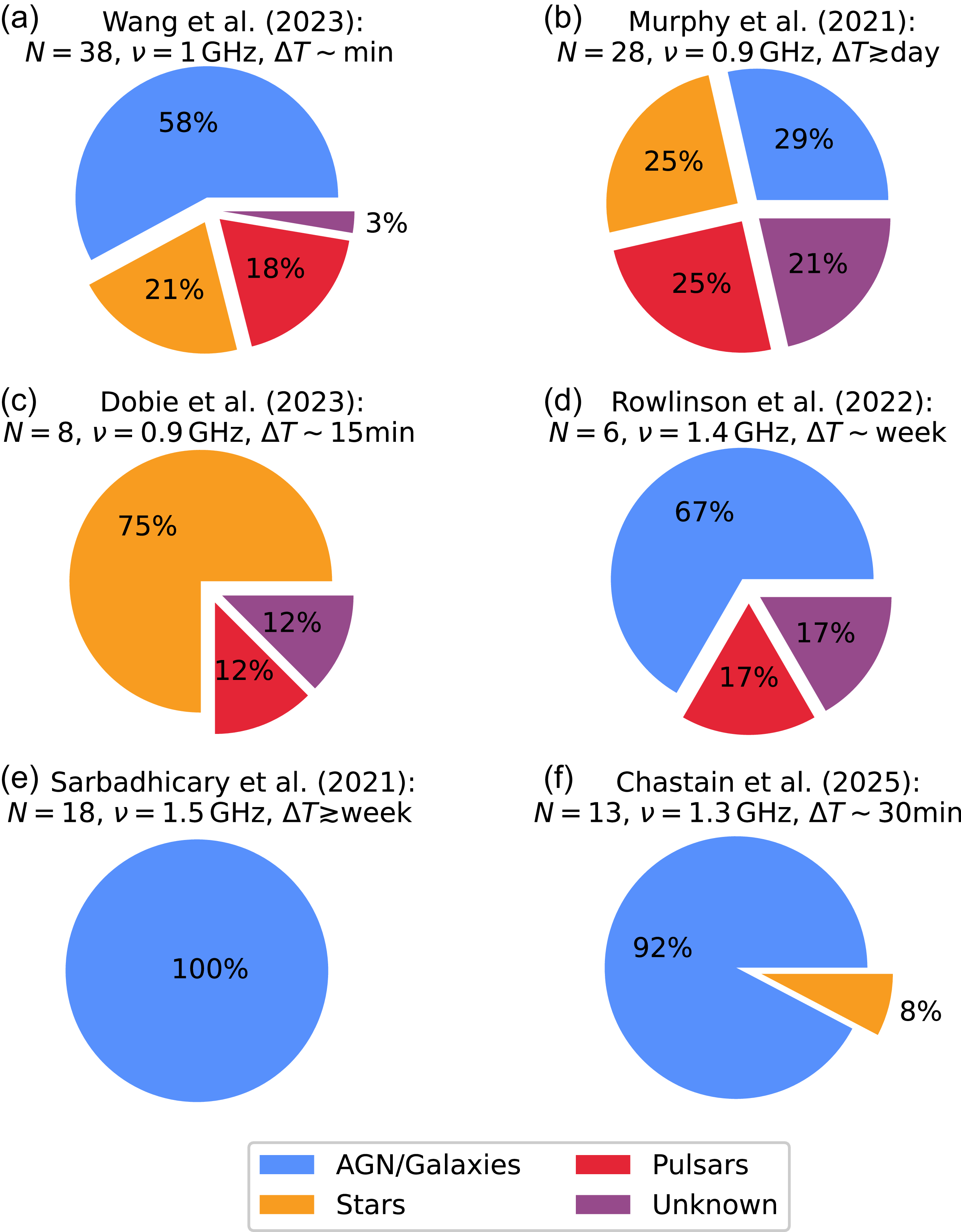
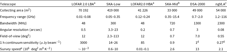
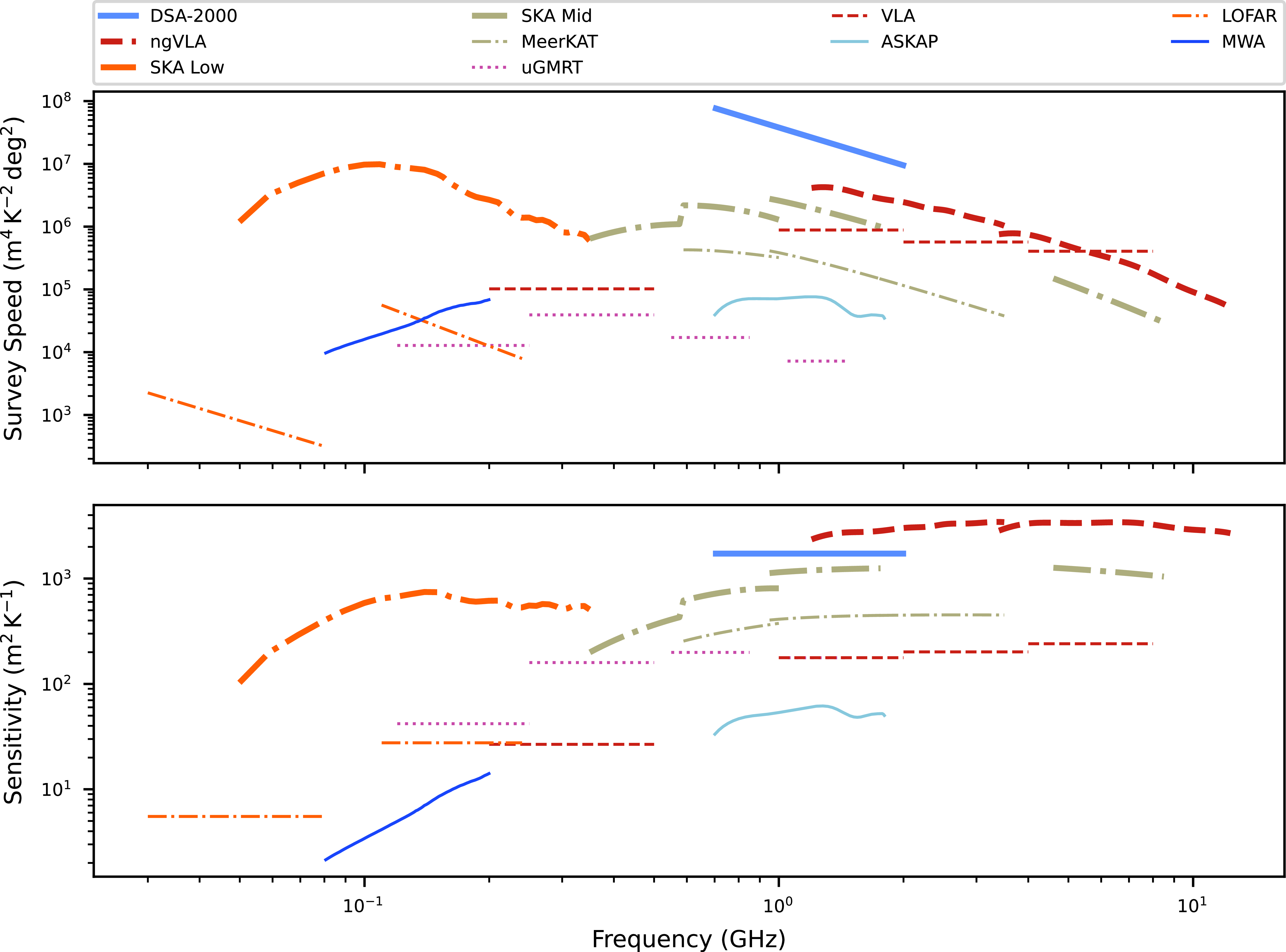


 Open access