


1 Introduction
Recent geochemical studies suggest that large environmental changes took place during the Late Ordovician in the interval leading up to and during the Late Ordovician mass extinction (LOME). These changes include a secular decline in global temperatures, most likely in response to reduced atmospheric pCO2, possibly related to ultramafic weathering or enhanced carbon burial (possibly due in part to land plant and marine green algal biomass expansion; see the recent review by Algeo & Shen Jun 2023) or some combination of those factors, which culminated in continental-scale glaciation. In addition, some recent work suggests that Late Ordovician cooling may have been interrupted by warming episodes created by the catastrophic outpouring of CO2 and H2S from massive volcanicity, although this remains controversial (e.g., Bond & Grasby Reference Bond and Grasby2017, Dahl et al. Reference Dahl, Hammarlund, Rasmussen, Bond and Canfield2021, Zhou Yu-ping et al. Reference Yu-ping, Yong and Wang2024). The Late Ordovician also apparently experienced large changes in sea level as well as changes in nutrient cycling, carbon burial, and phytoplankton community composition, among other possible effects. These oceanographic and nutrient cycling effects are manifest in pronounced facies changes, stable isotopic excursions, including the widely documented Hirnantian isotopic carbon excursion (HICE), as well as reported perturbations in nitrogen, sulfur, uranium, and others (e.g., Melchin et al. Reference Melchin, Mitchell, Holmden and Štorch2013, Harper Reference Harper2023, Young et al. Reference Young, Edwards, Ainsaar, Lindskog and Saltzman2023).
Testing alternative hypotheses about the direct cause (or causes) of the LOME requires a clear and precise understanding of the timing, rate, and selectivity of the extinctions. As the current, regionally heterogeneous response to global warming demonstrates, however, no single section or region can provide an adequate proxy for global change. Thus, a full assessment of mass extinction dynamics must include a global analysis that integrates the individual paths of biotic response to the local facies and habitat manifestations of global environmental change, while also compensating as much as possible for the artifacts that arise from sequence stratigraphic effects on the preserved record (Holland & Patzkowsky Reference Holland and Patzkowsky2015, Holland Reference Holland2016, Zimmt et al. Reference Zimmt, Holland, Finnegan and Marshall2021, Holland Reference Holland2023). Yet many recent papers regarding the LOME have nonetheless extrapolated from small regional studies or even single sections to global-scale conclusions about Late Ordovician climate and mass extinctions while taking little or no account of local-scale basin dynamics or potential sequence stratigraphic effects on the record. It is not surprising, then, that the literature is now replete with conflicting explanations for this momentous episode in Earth history.
The specific goals of the present research are, first, to use the paleotropical synthesis of graptolite species occurrence data employed by Melchin et al. (Reference Melchin, Sheets, Mitchell and Fan2017) to assess the rate, timing, and selectivity of graptolite species turnover within a global, high-resolution, sample-based composite timescale; and secondly, to apply that sample-based composite timescale to make a precise set of comparisons between the resulting global history and the patterns of environmental change in local sections across the paleotropics and thereby test the principal alternative hypotheses about the drivers of mass extinction during the Late Ordovician.
1.1 Background
From their analysis of the Late Ordovician record, Brenchley et al. (Reference Brenchley, Marshall and Carden1994, Reference Brenchley, Marshall and Underwood2001, Reference Brenchley, Carden and Hints2003) suggested that the Late Ordovician mass extinction comprised two pulses, and this interpretation has been widely (if somewhat imprecisely) adopted in studies of the LOME (e.g. Sheehan Reference Sheehan2001, Finnegan et al. Reference Finnegan, Heim, Peters and Fischer2012b, Melchin et al. Reference Melchin, Mitchell, Holmden and Štorch2013, Harper et al. Reference Harper, Hammarlund and Rasmussen2014, Luo Gen-ming et al. Reference Gen-ming, Algeo and Ren-bin2016, Zou Cai-neng et al. Reference Cai-neng, Zhen and Poulton2018a, Bond & Grasby Reference Bond and Grasby2020, Hu Dong-ping et al. Reference Dong-ping, Meng-han and Xiao-lin2020, Chen Yan et al. Reference Yan, Chun-fang, Zhen and Wei2021, Kozik et al. Reference Kozik, Gill, Owens, Lyons and Young2022a, Harper Reference Harper2023, Hu Rui-ning et al. Reference Rui-ning, Jing-qiang and Wen-hui2024, among many others). Not coincidentally, the Late Ordovician glacial interval, although part of a long-term and gradually increasingly severe glacial epoch, is now widely regarded as having culminated in two major glacial advance cycles within the Hirnantian itself separated by a brief warm period that took place early in the interval of the Metabolograptus persculptus Biozone (reviewed in Ghienne et al. Reference Ghienne, Desrochers and Vandenbroucke2014; see Fig. 1). Nonetheless, Chen Xu et al. (Reference Xu, Melchin, Sheets, Mitchell and Jun-xuan2005b), based on species occurrence data from a set of four sections in South China, found that graptolite extinction in this interval was dominated by a single early Hirnantian pulse. Likewise, Wang Guang-xu et al. (Reference Guang-xu, Ren-bin and Percival2019) concluded from their global review of Late Ordovician faunas that turnover among brachiopods during the LOME was dominated by a pulsed, although somewhat diachronous, extinction around the beginning of the Hirnantian that was then followed by an extended period of turnover as the newly evolved faunas tracked the changing Hirnantian and early Rhuddanian environments. These results reinforce the concerns, highlighted by Holland and Patzkowsky (Reference Holland and Patzkowsky2015), that we should have about the degree to which the “two pulse” model is a real feature of the LOME rather than an artifact generated by the effects of glaciation on the rock record itself.
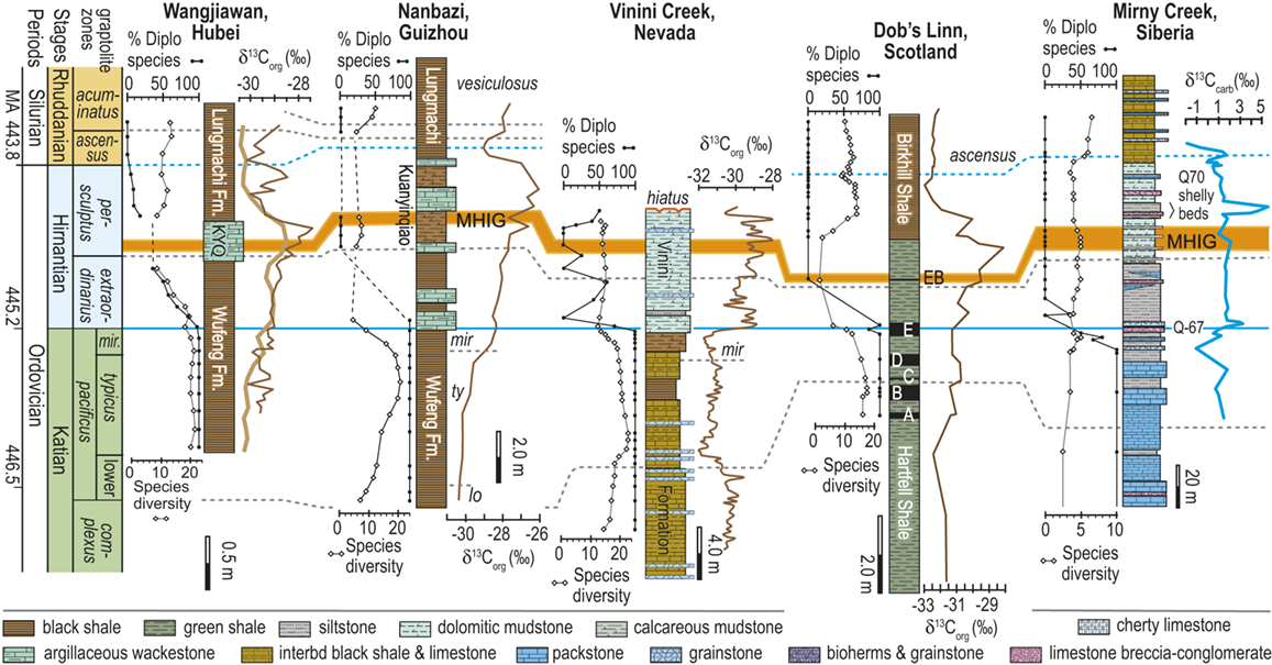
Observed trajectories in graptolite species diversity and turnover in clade composition relative to lithostratigraphy and the Hirnantian carbon isotopic excursion (HICE) at five intensively studied sections from across the paleotropics (see Fig. 2 for site locations). Sections exhibit distinctly different patterns of graptolite faunal turnover relative to lithological change and the trajectory of the C-isotopic excursion, as described later in the Element. Sections shown, from left to right: Wangjiawan (25) and Honghuayuan/Nanbazi (12) in South China; Vinini Creek (24) and Dob’s Linn (6) on opposite sides of Laurentia; and Mirny Creek (19) in Kolyma. Full names of graptolite biozones (in descending order, including abbreviations): Cystograptus vesiculosus Biozone, Parakidograptus acuminatus Biozone, Akidograptus ascensus Biozone, Metabolograptus persculptus Biozone, Metabolograptus extraordinarius Biozone, Paraorthograptus pacificus Biozone, Diceratograptus mirus Subzone, Tangyagraptus typicus Subzone (ty); lower unnamed subzone of P. pacificus Biozone (lo), Dicellograptus complexus Biozone. Other abbreviations: A,B,C,D,E, Anceps Bands A–E; EB, Extraordinarius Band; KYQ, Kuanyinqiao Beds; MHIG, mid-Hirnantian interglacial episode. Placement of the MHIG is based on a combination of geochemical and faunal data; see Appendix A for additional information about the occurrence of Metabolograptus persculptus in the EB at Dob’s Linn and Appendix B for data sources.
1.1.1 Graptolites and the Late Ordovician Mass Extinction
Although meaningful analyses of faunal dynamics have been conducted using genera, it is obvious that species-level data are preferable when the record is sufficiently complete. The graptolite fossil record is such a case (see, for example, Sadler et al. Reference Sadler, Cooper and Melchin2011). Based on their analysis of a global compilation of graptolite species ranges, Foote et al. (Reference Foote, Sadler, Cooper and Crampton2019, p. 1049) estimated that for the species that dwelt within the region of preserved Ordovician and Silurian strata, approximately “75% of Ordovician–Silurian graptoloid species have been sampled and that, of those known from more than one resolvable stratigraphic level, c. 85% of their original durations are represented by their composite stratigraphic ranges.” Foote et al. concluded that relative to other studied animal groups, graptolites have one of the most completely sampled fossil records.
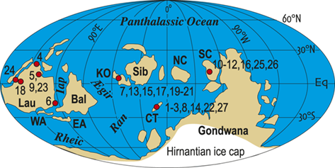
Additionally, as macrozooplankton, graptolites offer a unique perspective on environmental dynamics within the surface regions of the world’s oceans. Individual species are known to have been widely distributed across the paleotropics (Chen Xu et al. Reference Xu, Melchin, Jun-xuan and Mitchell2003, Boyle et al. Reference Boyle, Sheets and Wu2017) (Fig. 2) and, as such, their fates were likely to have been intimately intertwined with similarly global features of the Late Ordovician environment (Cooper et al. Reference Cooper, Rigby, Loydell and Bates2012, Reference Cooper, Sadler, Munnecke and Crampton2014, Crampton et al. Reference Crampton, Cooper, Sadler and Foote2016, Crampton et al. Reference Crampton, Meyers and Cooper2018). Observed graptolite species diversity in the paleotropics declined dramatically through the LOME from a peak of about 80 species known in mid Katian time (~ 446 Ma) to a Hirnantian nadir of about 20 species, barely 1.5 Myr later (Sadler et al. Reference Sadler, Cooper and Melchin2011). The composition of the faunas changed dramatically as well. Late Ordovician graptolite faunas were populated by species from two major clades: the Diplograptina and the Neograptina, which had diverged during the Darriwilian, approximately 15 Myr prior to the LOME events (Mitchell et al. Reference 74Mitchell, Goldman and Klosterman2007a, Reference Mitchell, Maletz and Goldman2009, Štorch et al. Reference Štorch, Mitchell, Finney and Melchin2011, Maletz Reference Maletz2023). In the late Katian, prior to the mass extinction, the Diplograptina were diverse and common throughout the paleotropics, where they comprised some 16 genera and were the only planktic graptolites present (Chen Xu et al. Reference Xu, Melchin, Jun-xuan and Mitchell2003, Goldman et al. Reference Goldman, Mitchell and Melchin2011, Melchin et al. Reference Melchin, Mitchell, Naczk-Cameron, Junxuan and Loxton2011, Goldman et al. Reference Goldman, Maletz, Melchin, Jun-xuan, Harper and Servais2014). The Late Ordovician Neograptina, in contrast, have a sparse fossil record and are only known from about ten species within two genera that were entirely confined to mid-high paleolatitude regions. However, coincident with the onset of the LOME in the latest Katian (i.e., within the Diceratograptus mirus Subzone of the P. pacificus Biozone), the Neograptina invaded the paleotropics and rapidly became the dominant graptolites (Chen Xu et al. Reference Chen, Jun-xuan, Melchin and Mitchell2005a, Goldman et al. Reference Goldman, Maletz, Melchin, Jun-xuan, Harper and Servais2014, Sheets et al. Reference Sheets, Mitchell and Melchin2016). By the end of the Hirnantian, the Diplograptina were entirely extinct (Melchin & Mitchell Reference Melchin, Mitchell, Barnes and Williams1991, Melchin Reference Melchin1998, Chen Xu et al. Reference Chen, Yuan-dong and Jun-xuan2006b, Finney et al. Reference Finney, Berry and Cooper2007, Goldman et al. Reference Goldman, Mitchell and Melchin2011, Bapst et al. Reference Bapst, Bullock, Melchin, Sheets and Mitchell2012).
Location map of 27 Late Ordovician to early Silurian graptolite-bearing sections studied here. Paleoplates from which data were used in the present study are labeled with the following abbreviations: Bal, Baltica; CT, Chu Ili-Tien Shan terrane; EA, East Avalon terrane; Iap, Iapetus Ocean; KO, Kolyma-Omolon terrane, Lau, Laurentia; NC, North China; SC, South China; WA, West Avalon terrane. Sites numbered as in Melchin et al. (Reference Melchin, Sheets, Mitchell and Fan2017); see Appendix 2 for data sources and sample-by-sample species occurrence data from these sites.
1.1.2 Distinguishing the Local and the Global
In general it appears that the macroevolutionary rates and clade turnover in graptolite faunas exhibit long-term rhythms that are comparable in duration with global Milankovitch-driven climate cycles (Crampton et al. Reference Crampton, Meyers and Cooper2018). Graptolite species turnover rates shifted to higher values during the LOME, in synchrony with the HICE and Hirnantian glaciation, and those elevated rates then persisted for the remainder of the clade’s history (Cooper et al. Reference Cooper, Sadler, Munnecke and Crampton2014, Crampton et al. Reference Crampton, Cooper, Sadler and Foote2016). Those results clearly implicate climate oscillations as a major driving force in graptolite extinction and several prior studies have proposed specific ties between graptolite ecology and the likely effects of Hirnantian climate change that could account for their extinction during the LOME (Melchin & Mitchell Reference Melchin, Mitchell, Barnes and Williams1991, Chen Xu et al. Reference Xu, Melchin, Sheets, Mitchell and Jun-xuan2005b, Finney et al. Reference Finney, Berry and Cooper2007). Nevertheless, the precise global pattern of timing and rate of turnover in graptolite faunas relative to Late Ordovician environmental change has not been well characterized at a temporal resolution sufficient to assess the degree of synchrony with the Hirnantian glacial advance and retreat cycles or other paleoenvironmental changes through that interval. Furthermore, regional and local-scale environmental effects (including but not limited to those associated with preserved facies shifts or hiatuses) have overprinted the record of global climate change. For instance, detailed local records of graptolite species turnover relative to the HICE and the mid-Hirnantian interglacial episode (which may provide approximate, independent measures of synchroneity among sections – see Holmden et al. Reference Holmden, Mitchell and LaPorte2013, Melchin et al. Reference Melchin, Mitchell, Holmden and Štorch2013, Ghienne et al. Reference Ghienne, Desrochers and Vandenbroucke2014) reveal disparate patterns of change in species diversity and faunal composition. These patterns may be grouped broadly into three sets (Figs. 1, 2):
Abrupt loss of all graptolites coincident with early Hirnantian facies change; examples include sections at Blackstone River, Laurentia [site 4], Ojsu Spring, Kazakhstan [22] and Ludiping, South China [16].
Graptolites remain common in the Hirnantian strata but faunas undergo a rapid loss of diversity and abrupt replacement of diplograptines by neograptines through the Katian-Hirnantian transition interval (ex: Vinini Creek, Laurentia [24], Mirny Creek, Siberia [19], Durben well, Kazakhstan [8], Honghuayan, South China [12]).
Faunas show an extended period of species diversity decline and clade replacement over the course of the latest Katian to mid-Hirnantian – namely through the entire first Hirnantian glacial megacycle (ex: Wangjiawan, South China [36], Dob’s Linn, Laurentia [6]).
In all of these cases diversity decline commences in the mid to upper part of the uppermost Katian Paraorthograptus pacificus Biozone; roughly in step with the onset of the HICE, however, the disappearance of species is earlier and more rapid in the more on-shore sites and latest in the more oceanic sites (see Sheets et al. Reference Sheets, Mitchell and Melchin2016, figs. S4, S5). Nonetheless, species losses are present in the deep sites that do not appear to be purely a result of facies and habitat displacement (e.g., at Vinini Creek, Sheets et al. Reference Sheets, Mitchell and Melchin2016), and at several of these sites species that appeared to go extinct in this initial pulse reappear as Lazarus taxa in the Metabolograptus persculptus Biozone in association with the falling limb of the HICE in the upper Hirnantian (Štorch et al. Reference Štorch, Mitchell, Finney and Melchin2011). Thus, many of the apparent early Hirnantian losses may be artifacts of sampling or habitat displacement or both (Mitchell et al. Reference Mitchell, Sheets and Belscher2007b) rather than true extinctions, consistent with sequence stratigraphic considerations (Holland & Patzkowsky Reference Holland and Patzkowsky2015, Holland Reference Holland2016, Reference Holland2023).
This ambiguity about the timing of extinctions is amplified by the individual failures of even these well-studied sections. Two examples will suffice here. The Mirny Creek section (the most complete and most fossiliferous of the seven Omulev Uplift sections studied in detail by Koren et al. Reference Koren, Oradovskaya, Pylma, Sobolevskaya and Chugaeva1983) is orders of magnitude thicker than the other principal graptolite-bearing Late Ordovician sections, and graptolites are rare in the Mirny Creek strata (Fig. 1). Most species are represented in each of the Omulev region collections by one to five specimens (Koren et al. Reference Koren, Oradovskaya, Pylma, Sobolevskaya and Chugaeva1983), despite a cumulative collection effort amounting to 20 person-months (T. Koren’ personal communication to CEM, 2005). Thus, it is likely that only the most common species were recovered, and that if some diplograptine species persisted into the Hirnantian there as rare individuals (see Koren’ & Sobolevskaya Reference Koren’ and Sobolevskaya2008), as we know they did elsewhere, these relict species almost certainly would not have been recovered.
The late Katian and early Hirnantian record at the Dob’s Linn section, which contains the global stratotype for the base of the Silurian System and has figured prominently in discussions of the LOME, is even more highly incomplete. Graptolite faunas of the late Katian P. pacificus Biozone, although reasonably diverse (Fig. 1), are recoverable from only two relatively thin black shale intervals (Anceps Band C and D; Williams Reference Williams1982). This zone has an estimated duration of some 1.8–3.38 My in the GTS 2012 and 2020 timescales, respectively (Cooper & Sadler Reference Cooper, Sadler, Gradstein, Ogg, Schmitz and Ogg2012, Goldman et al. Reference Goldman, Sadler, Leslie, Gradstein, Ogg, Schmitz and Ogg2020). The base of the Hirnantian is not recorded precisely, but most likely lies somewhere between Band D and Band E, which contains the first record of Metabolograptus extraordinarius, and thus probably corresponds to a level within the early Hirnantian M. extraordinarius Biozone (Williams Reference Williams1982, Melchin et al. Reference Melchin, Holmden, Williams, Albanesi, Beresi and Peralta2003, Chen Xu et al. Reference Xu, Jia-yu and Jun-xuan2006a). Restudy of the very small fauna preserved within the overlying, ~ 2 cm-thick Extraordinarius Band indicates that it contains Metabolograptus persculptus and is thus of late Hirnantian, M. persculptus Biozone age (Melchin et al. Reference Melchin, Holmden, Williams, Albanesi, Beresi and Peralta2003; see also Appendix A of this Element for further details). Accordingly, Band E is the only level from which early Hirnantian graptolites may be recovered at Dob’s Linn. It is thick enough to be subsampled (Fig. 1) but nonetheless represents only a small portion of the total duration of this biozone. Furthermore, sedimentological evidence suggests that Band E was deposited during an interglacial episode (Armstrong & Coe Reference Armstrong and Coe1997), and is thus atypical of the glacial conditions that prevailed during the early Hirnantian. Thus, the critical late Katian to mid Hirnantian LOME interval is represented at this site by five samples, none of which appear to sample the first main glacial advance. Since resolving the order of a set of events requires at least as many samples as events, the record at Dob’s Linn is grossly insufficient to resolve the extinction history of the 17 species present in the P. pacificus interval there. It is surprising, therefore, to see graptolite diversity data from this section cited as evidence that a spike in Hg abundance at this site indicated that the mass extinction was caused by an abrupt pulse in volcanic activity (Bond & Grasby Reference Bond and Grasby2020). Such a causal relationship simply cannot be determined from those data.
From the foregoing it is clear that no single section, not even the best, can serve adequately as a proxy for the full environmental and evolutionary history that we seek to understand. Accordingly, we have compiled a global composite based upon the full record of graptolite species sightings, occurrence by occurrence, through 27 sections from across the paleotropics (Melchin et al. Reference Melchin, Sheets, Mitchell and Fan2017) and herein report on the pattern of graptolite turnover extracted from that composite. As we discuss more fully later, this high-resolution composite overcomes some of the failures of the record imposed by local sections and permits a close, and precisely timescaled comparison between geochemical environmental proxies from those sections and the composite macroevolutionary history of graptolites.
1.1.3 Sample-Based Graptolite Occurrence Dataset
The dataset that we employed for this study of graptolite species dynamics through the LOME is the same dataset employed in Melchin et al. (Reference Melchin, Sheets, Mitchell and Fan2017). It comprises 3,508 presence-absence records for 105 species from 633 collections distributed among 27 measured sections. The selected sections are those that exhibit relatively continuous sedimentation through the LOME interval, are rich in graptolites, and have been documented via detailed systematic study of those faunas. We have compiled this dataset from the published record of species occurrences; in several cases, however, we have augmented that record by additional collections from the sections (especially at Dob’s Linn) and, for most of these collections, by direct restudy of the original graptolite material. We have applied a uniform taxonomy to the species occurrences insofar as this is possible based on the published record and our ability to restudy those collections. The study sites occur within the region ~ 20° north and south of the paleoequator and encompass approximately 210° in paleolongitude. Data from higher-latitude regions are available from very few sites and include too few species in common with the paleotropical faunas to be reliably integrated by the automated sequencing approach that we employed to form a unified composite of species occurrences (see the “Methods” section later in the Element). Thus, although conceptually of value in the present context, these occurrences are not treated quantitatively herein.
The number of species that cooccur within individual samples varies considerably among the samples employed for this study and most samples contain few species (Fig. 3), some of which are confined to single sections. Such species are not stratigraphically informative and the age of the samples in which they occur is constrained only by the presence of other, more widely shared species – either in those samples or in other samples in the same section. In the present study we employ the occurrences of stratigraphically informative species to form an ordered sequence of samples by the methods described later in the Element. The ranked frequency distribution of informative species diversity per sample follows the expected negative log-normal distribution for sampled species diversity more generally, with an R2 of 0.9627 between informative species diversity and the log of the number of samples. The median per-sample diversity of stratigraphically informative species is 4.0 (Fig. 3A). Similarly, histograms of species sighting frequency (Fig. 3B) indicate that most stratigraphically informative species occur in few samples (Fig. 3B), consistent with the findings of Foote et al. (Reference Foote, Sadler, Cooper and Crampton2019); however, Fig. 3B also shows a second mode of species that are moderately to widely occurring with 50 or more occurrences in the sampled sections. The median number of occurrences per species ranges from three to 12 among biozones in the latest Ordovician and earliest Silurian, which, although somewhat variable, shows no obvious trend through the study interval, particularly when treated as sightings per million years (Fig. 3B; we describe the sources of the zone durations in Section 2.2). Furthermore, the number of sightings per million years for individual species during the Hirnantian are similar to the overall median for the dataset. Accordingly, the available data appears to be sufficient to warrant the analyses described in the following sections.
A Histogram of the number of stratigraphically informative species per sample (ordinate). Thirty-five samples contain only species that are not shared with samples from other sections (i.e., species that are unique to single localities) and thus have zero informative species. The position in the ordinal composite of such samples is constrained only by samples above or below them that do contain stratigraphically informative species. The ordinal position of 67 percent of samples is constrained by the joint occurrence in those samples of three or more species and that of slightly less than half is constrained by five or more. B, Histogram of the sighting frequency (i.e., the number of recorded occurrences) for each species through its full range within the dataset, together with tabulated median, median/myr, and maximum sighting frequencies within individual biozone intervals and the study interval as a whole; for example, Appendispinograptus supernus (which is the most widely reported species in the set) is reported in 200 samples within the full dataset and in 145 samples within the P. pacificus Biozone.
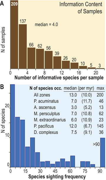
Figure 3 Long description
A. The upper panel presents a histogram of the number of species within samples as a documentation of the diversity values recorded are counts of the number of stratigraphically informative species, i.e., species at occur in more than one stratigraphic section. The histogram contains 11 bins, each with an interval width of 2, and they exhibit a monotonically decreasing frequency value as sample diversity increases from one to a maximum of 22. Thus, the left-most is also the highest column and represents the number of samples that contain 1 or 2 stratigraphically informative species, and the last (eleventh) represents samples with 23 or 24 species. The number of samples for each of these cohorts is 209, 137, 66, 62, 56, 39, 26, 20, 10, 5, and 3. The median number of informative species per sample is 4.0.
B. The lower panel also contains a histogram of the number of occurrences per species (species sighting frequency) for the data set as a whole, as well as a small table of statistics about the number of occurrences per species within each graptolite biozone. The histogram contains 19 bins, each with an interval width of 5. The largest number of species (28) have one or two occurrences, and the number of species with increasing sighing frequency falls rapidly to a low of one species that has 41 to 45 occurrences. This is followed by a slight increase in the number of species with yet higher sightings to a secondary mode of four with 61 to 65 occurrences, following which species with higher sightings again become fewer, with none that have 86 to 90 occurrences. The overflow bin of species with greater than 90 occurrences includes 10 species, the most common of which, Appendispinograptus supernus, is recorded in 200 samples within the full dataset. Inset within the area of the figure is a table that reports three measures of the species sighting frequency distribution: median, median/myr, and maximum observed values. Values are given for the whole data set and for each biozone, from youngest to oldest: all zones 13.0 10.0 200 P. acuminatus 7.0 11.7 46 A. ascensus 3.0 5.2 13 M. persculptus 7.0 10.8 62 M. extraordinarius 6.0 10.9 23 P. pacificus 12.0 6.7 145 D. complexus 7.5 9.1 36
2 Methods
2.1 Determining Species Ranges
We determined graptolite species ranges by use of an automated sequencing approach called Horizon Annealing (Sheets et al. Reference Sheets, Mitchell and Izard2012, Melchin et al. Reference Melchin, Sheets, Mitchell and Fan2017). Horizon Annealing (HA) is a modification of the more widely used constrained optimization (CONOP) approach developed by P. M. Sadler and colleagues (Kemple et al. Reference Kemple, Sadler, Strauss, Mann and Lane1995, Sadler & Kemple Reference Sadler, Kemple, Cooper, Droser and Finney1995, Sadler et al. Reference Sadler, Kemple, Kooser and Harries2003). These automated sequencing approaches are based on the contention that the first and most fundamental task for measuring species durations in the fossil record is to determine the order of those events – the species’ global first and last appearance events (FAD and LAD, respectively). That set of ordered events is then scaled relative to a convenient timescale – generally one measured in millions of years and derived from geochronologically dated samples that can also be placed within the ordinal sequence of events (see the discussion in Goldman et al. Reference Goldman, Sadler, Leslie, Gradstein, Ogg, Schmitz and Ogg2020 and references cited therein).
Detailed descriptions of the HA ordination process are given in Sheets et al. (Reference Sheets, Mitchell and Izard2012) and Melchin et al. (Reference Melchin, Sheets, Mitchell and Fan2017), but briefly, both the HA and CONOP automated sequencing techniques seek to determine the global ordinal sequence of a set of species’ FADs and LADs in such a way that the ordination minimizes the sum of all the species ranges while also accounting for the observed overlaps among the species ranges. CONOP does this by explicitly ordering species’ FADs and LADs based on the order of these events within individual sections. HA, in contrast, orders all available samples (not just range ends) based on the species contents of the samples (constrained by stratigraphic position within sections) and the implications of those occurrences for the overlap of species ranges, seeking to minimize the number of range overlaps while again accounting for all observed within-sample co-occurrences and range overlaps. The ordinal position of 67 percent of samples is constrained by the joint occurrence in those samples of three or more species and that of slightly less than half is constrained by five or more species (Fig. 3A).
For the purpose of sample ordination in HA, we may define the term “taxa” broadly to include not only species occurrences but also any other observable event that appears to have regional or global chronostratigraphic significance, such as volcanic ash layers, unique lithostratigraphic markers (such as sequence boundaries or other distinctive event beds), or chemostratigraphic events, among other possibilities. In the process of constructing the ordination employed here, Melchin et al. (Reference Melchin, Sheets, Mitchell and Fan2017) included the Kuanyinchiao Bed, which is a lithostratigraphically distinctive unit that is widely distributed in the mid-Hirnantian succession of South China (Chen Xu et al. Reference Chen, Jia-yu, Yue and Boucot2004, Chen Qing et al. Reference Qing, Jun-xuan, Melchin and Lin-na2014) as well as the rising and falling limbs of the HICE, each treated as discrete taxa (see Melchin et al. Reference Melchin, Sheets, Mitchell and Fan2017 for further discussion).
For this analysis all of the samples and taxa (whether graptolite species or other event types) were weighted equally. This approach did not privilege ‘key’ or zonal index taxa and did not assume that the FAD of M. extraordinarius (or of any taxon) is everywhere the same age. Thus, the ordination employed here is an unbiased maximization of all the available information in the dataset about the sequence of graptolite FADs and LADs and does not rely upon any particular assumption about the correspondence of species appearances or disappearances to Late Ordovician glacial or other events (such as the HICE) or to the timing of those events. Each is allowed to find its own level, as it is best fit by the data overall. The resulting ordination integrates species occurrences across regional facies gradients and paleoplates within a sequential framework that maximizes the fit of all the available data to the modeled species durations. It is this relaxation of the assumption of synchroneity among species range ends and the integration of occurrences across regional facies gradients (from on-shore sites to outer shelf and slope sites) that maximizes the likelihood of overcoming taxon range truncations imposed by eustatic changes in sea level and the resulting incompleteness of the geological record (Holland Reference Holland2020, Zimmt et al. Reference Zimmt, Holland, Finnegan and Marshall2021).
The Horizon Annealing composite employed here has three additional features that are noteworthy in the present analyses. Firstly, the HA composite is amenable to jackknife analysis, in which sections are removed from the dataset, one section at a time, and the ordination solution is then recalculated. The standard deviation of the variation in the placement of each sample across the set of jackknife replicates may serve as a measure of uncertainty in the position of that sample in the ordination (Melchin et al. Reference Melchin, Sheets, Mitchell and Fan2017). This uncertainty naturally differs among samples based on the faunal content of the sample and its stratigraphic context. In the present case, the median standard deviation in horizon placements (omitting the lowest and highest 16 percent of ordinal positions, where variance in position appears to be constrained by edge effects) is 8.14 ordinals. This jackknife uncertainty value provides a useful gauge of the reliable resolution of the ordination and thus served as a guide to selecting a minimum temporal bin duration for our turnover analysis.
Secondly, because the analyzed sample set retains all occurrences of each of the graptolite taxa in the studied sections, rather than only their FADs and LADs, the final ordination includes information about the frequency with which taxa occur through the succession and among sites. That information, then, can be used to assess the likelihood of encountering an extant taxon in an observational interval. This is a key piece of information needed to refine estimates of species origination and extinction rates and to assess their interdependency with changes in completeness of the dataset through the glacial interval (Foote Reference Foote2001). We will return to this topic later in our discussion of Capture-Mark-Recapture analysis.
Thirdly, because HA orders samples rather than taxa, and because all samples from a given section must remain in their observed stratigraphic order, HA can carry any sample through the ordination process, irrespective of whether that sample contains species or other properties that are informative about their position in the ordinal sequence. Thus, the HA composite can include occurrences of species that are unique to single samples or sections in so far as these horizons are constrained by other horizons in the same sections. More importantly, this property of HA allows ordinal placement of samples that bear locally unique chemostratigraphic, paleoenvironmental, or lithostratigraphic information of value to the interpretation of the geological and evolutionary history of the species of concern. We make use of this feature in our discussion of the possible environmental causes of the observed graptolite species turnover. Taken together these features provide a well-grounded evidentiary basis from which to assess species turnover dynamics and facilitate discrimination between local and global patterns of turnover and their relationships to paleoenvironmental change.
2.2 Temporal Scaling of the Ordinal Composite
In the HA composite, each sample occupies a unique position in the ordered sequence of samples. In order to provide species ranges in millions of years, we must convert that ordinal sequence to a timescaled succession. We estimated median durations (in Myr) for D. complexus through C. vesiculosus biozones based on those given in GTS2012 (Cooper & Sadler Reference Cooper, Sadler, Gradstein, Ogg, Schmitz and Ogg2012, Melchin et al. Reference Melchin, Sadler, Cramer, Gradstein, Ogg, Schmitz and Ogg2012) and combined those estimates with additional estimates of zone duration. These latter include estimates derived from geochronological age dates (Ling Ming-xing et al. Reference Ming-xing, Ren-bin and Guang-xu2019, Du Xue-bin et al. Reference Xue-bin, Yong-chao and Dan2020) and astrochronological interval durations (Lu Yang-bo et al. Reference Yang-bo, Chun-ju and Shu2019, Jin Si-ding et al. Reference Si-ding, Hu-cheng and Xing2020, Zhong Yang-yang et al. Reference Yang-yang, Huai-chun and Jun-xuan2020). The 3.38 Myr duration of the P. pacificus Biozone in the GTS2020 timescale (Goldman et al. Reference Goldman, Sadler, Leslie, Gradstein, Ogg, Schmitz and Ogg2020) is unusually long compared to that in the GTS2012 and to other estimates of the duration of this zone. Consequently, we did not use the GTS2020 zone durations in our timescaling process although we did adopt 443.07 Ma as the current best estimate of the age of the beginning of the Silurian. After determining the median duration of each zone, we placed the position of zone boundaries in the composite based on the ordinal position of the FAD of the key index taxon for each zone. Working from the GTS2020 estimated age of the beginning of the Silurian (i.e., the start of the A. ascensus Biozone; 443.07 Ma), we used the median durations to provide estimates of the geochronological age of each of the other zonal boundaries. Finally, we used linear interpolation to convert the ordinal positions of all horizons within each of the biozones to a corresponding geochronological age. The resulting intervals in the scaled composite that encompass the set of samples from each of the graptolite biozones or subzones are chronostratigraphic units – that is, they are our best estimate of the particular intervals of geological time during which the strata of the biozones were deposited. Following the standard terminology of the International Commission on Stratigraphy, we refer to these intervals in our scaled composite as chrons and subchrons and label them by the trivial epithet of the eponymous species of the corresponding biozone (e.g., “Extraordinarius Chron,” and so on).
We divided the resulting temporally scaled composite into twenty-four analytical intervals (referred to herein as bins), each with a duration of 210,000 years.Footnote 1 These temporal bins contain an average of 24 horizons and a range of 10 and 61 horizons per bin. Thus, all bins are longer than the jackknife uncertainty in the ordinal position of horizons and most are several times longer. Most of the biostratigraphic units recognized through the latest Ordovician and early Silurian formed during intervals on the order of 0.6 Myr and are represented in the dataset by two or three bins. The relatively long P. pacificus Chron (with its three subchrons), which has a median estimated duration of 1.8 Myr in the datasets we employed, is represented by eight or nine bins. The temporal resolution of our chosen binning is comparable to that which Chen Xu et al. (Reference Xu, Melchin, Sheets, Mitchell and Jun-xuan2005b) employed in their analysis of graptolite species turnover in the Yangtze Platform region of China and similar to the duration of the moving window that Copper et al. (Reference Cooper, Sadler, Munnecke and Crampton2014) and Crampton et al. (Reference Crampton, Cooper, Sadler and Foote2016, Reference Crampton, Meyers and Cooper2018) employed in their analyses of graptolite species diversity and turnover.
Recognizing that uncertainty in the ordinal location of events in the Melchin et al. (Reference Melchin, Sheets, Mitchell and Fan2017) HA composite is substantial relative to the resolution in our binning scheme, we constructed two alternative placements of the 24 equal-duration bins relative to the composite sequence: binning schemes, B1 and B2 (Fig. 4). We also employed a third, substantially different binning scheme, B3, that we describe further later. These alternatives provide an indication of the effects of bin boundary placement on the estimated rates and timing of species turnover. In the first binning scheme, B1, we placed the bin boundaries such that the first bin spans the beginning of the Complexus Chron and the start of the 14th bin coincides with the global FAD of Metabolograptus extraordinarius (i.e., to the start of the Extraordinarius Chron). That level in the composite is equivalent, within error, to the position of the Hirnantian GSSP at Wangjiawan, South China, which also lies within B1 bin-14. Thus, bin B1-14 represents the beginning of the Hirnantian Age as formally defined (see Melchin et al. Reference Melchin, Sheets, Mitchell and Fan2017). In B2, we offset the bins upward by approximately one-half a bin so that the start of the first bin coincides with the FAD of D. complexus (= the beginning of the Complexus Chron) and the FAD of M. extraordinarius falls within B2-13. This bin placement retains the Hirnantian GSSP level within B2-14, and thus, does not impose synchroneity between the global first appearance of M. extraordinarius and the start of the Hirnantian Age.
Timescale employed for the analysis of graptolite species diversity and turnover during the late Katian and Hirnantian ages (Late Ordovician Epoch) to early Rhuddanian Age (Llandovery Epoch, Silurian Period). Geochronological ages (in Ma) and chronozone durations employed herein based on the GTS2020 timescale (Goldman et al. Reference Goldman, Sadler, Leslie, Gradstein, Ogg, Schmitz and Ogg2020) and data from the literature (see Table 1 and text for discussion). Uncertainty error bars (±2σ) shown for the geochronological age of the beginning of the Silurian, duration of the Hirnantian (based on calculations herein), the first appearance datum (FAD) of Metabolograptus extraordinarius and the Hirnantian GSSP in the timescale, along with the location of the rising limb, peak, and falling limb of the widespread Hirnantian d13C isotopic excursion (HICE), all based on the ordinal position of global events, including the FADs and LADs of the rising and falling limbs of the HICE, in the Melchin et al. (Reference Melchin, Sheets, Mitchell and Fan2017; see also Appendix B) composite. Also shown is the temporal alignment of the three sets of 24 analytical bins (B1-B3) employed for the diversity analysis. All bins in B1 and B2 are 210 Kyr in duration but encompass different numbers of horizons (N from 10–52); those of B3 are variable in duration (80–420 Kyr) but each includes 24 horizons. Hirnantian bins are shaded and the beginning of the first Hirnantian-aged bin in the B1 set (B1-14) is aligned with the beginning of M. extraordinarius Chron, whereas the beginning of the first bin in B2 and B3 is aligned with the beginning of the D. complexus Chron. Based on the placement of samples marking the LAD of the rising limb and FAD of the falling limb of the HICE (see Melchin et al., Reference Melchin, Sheets, Mitchell and Fan2017 for discussion of the coding of the segments of the HICE) the late HICE peak displayed at Wangjiawan (site 25) and Dob’s Linn (site 6) and shown in Fig. 1, occupies an interval from about 443.73 ± 0.19 Ma, coeval with the start of the Persculptus Chron, to about 443.62 ± 0.10 Ma at the beginning of the falling limb of the HICE in mid Persculptus Chron time. At other sites, such as Vinini Creek (site 24) and Blackstone River (site 4), the broader HICE peak commences near the beginning of the Hirnantian
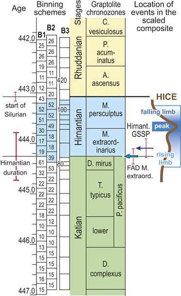
The offset between the B1 and B2 schemes results in differences in the total number of bins that incorporate Hirnantian samples (six in B1 and seven in B2) and changes the extent to which the 24 bins extend into the early Silurian (Fig. 4). They also shift slightly the overlap between the Mirus Subchron and our bins. This is noteworthy because previous work on the LOME indicates that both the turnover events and related environmental changes that are associated with the LOME (including disruptions of the carbon system reflected in the HICE) accelerated during the Mirus Subchron. That upsurge in the pace of LOME-related change will thus appear in slightly different places among the three binning schemes; it occupies the 12th and 13th bins in B1, only the 12th bin in B2, and the 9th–11th bins in B3 (more on this last scheme later).
Foote (Reference Foote, Erwin and Wing2000) demonstrated that short-term changes in sampling intensity or probabilities of taxon recovery affect estimates of rates of origination and extinction. As we noted earlier, the number of samples included in each bin differs among bins and it also differs among binning schemes for similar points in the time series (Fig. 4). This arises because the biozones that we used to scale the composite themselves differ in duration and because the number of samples within each biozone differs substantially among biozones independently of their duration (Table 1). Consequently, the temporal spacing of the ordinal horizons differs through the time series. We have used two different approaches to assess the impact of the differing levels of sampling among bins. First, by shifting bin boundaries to form the B1–B2 sets we not only altered the placement of environmental events relative to those boundaries (concentrating or spreading episodes), we also shifted the density of data within bins (Fig. 4) relative to those events. For instance, the four bins that span the beginning of the Hirnantian in B1 contain 32, 61,19 and 17 horizons, whereas those in B2 contain 22, 53, 39, and 18. We also constructed the B3 binning, in which each of the 24 bins contains exactly 24 horizons. Those bins also average 210 Kyr, as in the other two bin sets, but range in duration from 80 to 420 Kyr. This clearly shifts the density of data in a dramatically different way, equalizing sampling per bin at the cost of equal duration bins. Features of the turnover history of graptolites shared among these three different bin sets must necessarily be largely independent of related sampling effects, at least at the ~ 210 Kyr resolution of the dataset. An obvious alternative is to analyze the data via a method, such as capture-mark-recapture analysis, that directly addresses uneven rates of taxon recovery, which we describe in the following section.
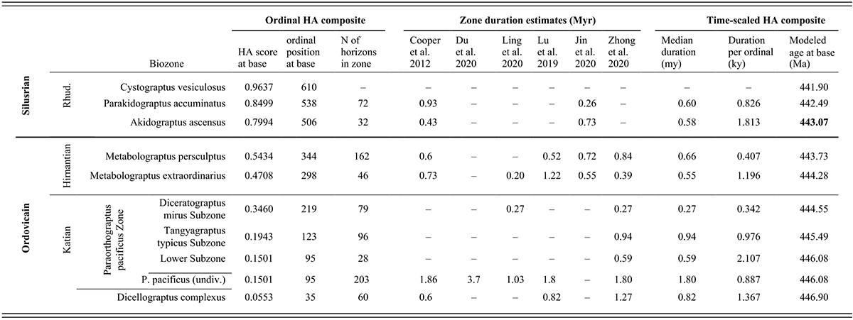
Table 1 Long description
This table presents data about the temporal duration and geochronological age of the stratigraphic intervals examined in this study. The chronostratigraphic interval examined is divided in the table into three sets of rows, highest (also the youngest) at the top and the lowest (oldest) at the bottom, and these intervals are labeled along the left side of the table. The highest of the three intervals considered here is the lower part of the Rhuddanian Stage, which is the basal part of the Silurian System. This interval contains three graptolite biozones that, also from highest to lowest, are the Cystograptus vesiculosus, Parakidograptus acuminatus, and Akidograptus ascensus biozones. The next oldest interval is the Hirnantian Stage, which is the highest of the Upper Ordovician Series, and consists of two biozones, the Metabolograptus persculptus and M. extraordinarius biozones, in descending order. The lower of the three examined intervals is the uppermost part of the Katian Stage, also part of the Upper Ordovician. That interval includes two biozones, the Paraorthograptus pacificus and Dicellograptus ornatus biozones, in descending order. The P. pacificus Biozone consists of three subzones, which, from highest to lowest, are the Diceratograptus mirus, Tangyagraptus typicus, and an unnamed lower subzone. Data for the P. pacificus Biozone are presented first for each subzone and then for the full biozone, undivided, which is then followed by data for the underlying D. ornatus Biozone.
The rest of the table consists of three blocks of information, all arranged in columns with a datum (or dash when data are missing) in each biostratigraphically labeled row. In the following description, the rows are identified for simplicity only by the trivial epithet of the biozone or subzone’s species name. Since the beginning of the Vesiculosus Biozone forms the top end of our analyzed time series, we present information only for that datum level.
The left-most data block consists of three columns that present information about the location of the biozones within the ordinal composite constructed by Horizon Annealing (H A). The first two columns (left to right) are, respectively, H A scores and H A ordinal positions. Both values reflect the location of individual samples (horizons) in that sequence, which has a total of 633 horizons and a set of scores that range from zero at the beginning of the ordination to 1.00 at its top. The ordinal position of the base of each biozone corresponds to the first appearance datum (F A D) of the eponymous species in the ordinal sequence. Since Tangyagraptus typicus and many associated species occur only in South China, the base of that sub-biozone and the succeeding Diceratograptus mirus subzone are determined only by the South China samples. Also listed in the third column, following the H A score and ordinal position, is the number of individual horizons (samples) included in each biozone. The data in this block of the table is as follows: vesiculosus 0.963665 610 (blank) acuminatus 0.8499 538 72 ascensus 0.7994 506 32 persculptus 0.5434 344 162 extraordinarius 0.4708 298 46 mirus subzone 0.3460 219 79 typicus subzone 0.1943 123 96 lower pacificus subzone 0.1501 95 28 pacificus undivided 0.1501 95 203 complexus 0.0553 35 60 Thus, the F A D of Dicellograptus complexus has an H A score of 0.0553, occurs as the thirty-fifth sample in the ordinated set, and the biozone includes 60 samples between this F A D and that of P. pacificus at the ninety-fifth ordinal position.
The next (central) block of the table presents estimates of the duration of each of the biostratigraphic units from six published sources that are here organized in six columns from left to right: Cooper et al. (2012), Du et al. (2020), Ling et al. (2020), Lu et al. (2019), Jin et al. (2020), and Zhong et al. (2020). The relatively sparse elements in this section of the table are as follows: vesiculosus (blank) (blank) (blank) (blank) (blank) (blank) acuminatus 0.93 (blank) (blank) (blank) 0.26 (blank) ascensus 0.43 (blank) (blank) (blank) 0.73 (blank) persculptus 0.6 (blank) (blank) 0.52 0.72 0.84 extraordinarius 0.73 (blank) 0.20 1.22 0.55 0.39 mirus (blank) (blank) 0.27 (blank) (blank) 0.27 typicus (blank) (blank) (blank) (blank) (blank) 0.94 lower pacificus subzone (blank) (blank) (blank) (blank) (blank) 0.59 pacificus undivided 1.86 3.7 1.03 1.8 (blank) 1.80 complexus 0.6 (blank) (blank) 0.82 (blank) 1.27
The final data block in this table presents three columns of calculated values for the time-scaled composite. From left to right, they are the median duration in millions of years of the geochronological interval occupied by each of the biostratigraphic units in the time-scaled composite, the average duration (in thousands of years) per ordinal within those intervals, and finally, the modeled age of the beginning of the intervals (in millions of years ago). These calculated values are vesiculosus (blank) (blank) 441.90 acuminatus 0.60 0.826 442.49 ascensus 0.58 1.813 443.07 persculptus 0.66 0.407 443.73 extraordinarius 0.55 1.196 444.28 mirus 0.27 0.342 444.55 typicus 0.94 0.976 445.49 lower pacificus subzone 0.59 2.107 446.08 pacificus undivided 1.80 0.887 446.08 complexus 0.82 1.367 446.90
In the text, we refer to these chronostratigraphic intervals as chrons, again labeled by the eponymous species’ trivial epithet. The quoted average duration per ordinal (interval length divided by number of ordinals in the interval) is then the temporal spacing applied to samples within those intervals prior to grouping (binning) horizons into the sets of 24 analytical intervals (bins), and so also quantifies the temporally variable information density through the sampled time series. Thus, the Complexus Chron has an estimated duration of 0.82 million years, a sample spacing of 1.367 kiloyears, and commences at 446.90 M a. The modeled starting dates of the intervals are simple additive combinations of the median estimated durations for the intervals, aligned in time with the beginning of the Silurian Period (443.07 M a), given in G T S 2020 (Goldman et al., 2020).
2.3 Estimation of Species Turnover Dynamics and Capture-Mark-Recapture Analysis
We employed two related approaches to quantifying species diversity, origination, and extinction rates. The first is the set of metrics (referred to as “face-value metrics” in the following text) advocated by Foote (Reference Foote, Erwin and Wing2000). These metrics are simple to calculate from presence-absence data and provide a relatively unbiased basis for the comparison of macroevolutionary rates and taxonomic diversity based on the fossil record. In this scheme, the chosen occurrence record is taken at face-value (hence the descriptor) and taxa are censused in a bin-by-bin scheme according to which of the bins’ boundaries they cross, as follows. Of the number of taxa that occur within a bin, some are bottom crossers (i.e., are known from older bins) and are symbolized as Nb; of those some will go extinct within the bin (= NbL, for bottom crosser and Last occurrence) and the remainder will pass into younger bins (cross the top boundary, =Nbt). Some of these latter may only be known from bins above and below but are treated as range-through taxa and included in the quantity Nbt. Additionally, some taxa within a bin cross (or are inferred to have crossed) the top of the bin (Nt), and these include species that first appeared (F) within that bin (NFt). Taxa that occur only within one bin (‘singletons’) cross neither bin boundary (NFL). Their number strongly depends upon bin duration and sampling completeness and thus increase the vulnerability of taxonomic diversity and evolutionary rate metrics to sampling artifacts (among other problematic effects; see Foote, Reference Foote, Erwin and Wing2000). Accordingly, we follow Foote’s practice and exclude singletons from our diversity and evolutionary rate calculations. Given these notations, estimated mean standing diversity is calculated as (NbL+NFt+2Nbt)/2 and estimated per capita origination (p̂) and extinction (q̂) rates (respectively) are –ln(Nbt/Nt)/ΔT and –ln(Nbt/Nb)/ΔT, where ΔT is the bin duration. For the sake of convenience, we plot the estimated diversity, origination, and extinction rate values at bin midpoints.
The Diplograptina went extinct in the late Hirnantian and we are unable to report an extinction rate for the bin in which the last known species occurs just as one cannot calculate an extinction rate for the final bin in a set of bins: it requires information that does not exist. Similarly, the Neograptina invaded the paleotropics in the latest Katian (Goldman et al. Reference Goldman, Mitchell and Melchin2011) and we therefore are unable to report an origination rate at that appearance or to distinguish in situ origination from immigration during this early segment of Neograptine resurgence in the paleotropics. Thus, the p̂ and q̂ time series reported from the face-value and CMR analyses for these clades are one bin shorter at both ends than the time series of species diversity with which they are associated in our figures and do not fully capture the timing of their initial immigration or final extirpation due to the logical limitations of binning and the calculations involved.
We calculated mean standing species diversity and per capita rates separately for each of the Late Ordovician to early Silurian graptolite clades (the Diplograptina and the Neograptina) following the systematic treatment of these graptolites given by Štorch et al. (Reference Štorch, Mitchell, Finney and Melchin2011) and Melchin et al. (Reference Melchin, Mitchell, Naczk-Cameron, Junxuan and Loxton2011) as well as for the full set of planktic graptolite species present in this interval. In order to provide additional phylogenetic context for the LOME events, we also counted the number of species appearances and disappearances in each bin for the three constituent subclades of the Diplograptina (the Dicranograptoidea, Diplograptoidea, and Climacograptoidea). We also separated the Neograptina into the clade Retiolitoidea and its subtending stem group, which we refer to as ‘stem-group neograptines,’ namely the Normalograptidae including species of the genus Normalograptus, and all other taxa that root below the common ancestor of the Retiolitoidea sensu Melchin et al. (Reference Melchin, Mitchell, Naczk-Cameron, Junxuan and Loxton2011). The Retiolitoidea is a diverse clade that in the LOME interval was represented overwhelmingly by M. extraordinarius and related species of the paraphyletic Neodiplograptidae (Metabolograptus, Neodiplograptus, Korenograptus, and Paraclimacograptus).
We have calculated the face-value metrics described earlier for each of the three different binning schemes as a rough gauge of the turnover history of graptolites through the LOME and also as a means to assess the role of binning (and its effect on sampling) on the calculated time series. These face-value metrics have a number of shortcomings, however. Most significantly for our present purposes, they do not incorporate information about the probability of sampling taxa through the study interval (Foote Reference Foote2003). If sighting probabilities are very unequal over time or space, or differ among taxa, then the face-value metrics will not capture the macroevolutionary dynamics accurately (Foote Reference Foote, Erwin and Wing2000, Reference Foote2001, Reference Foote2003). For instance, the omission of sighting information from the analyses forces one to assume that observed first and last occurrences represent the actual time of origin or extinction of the taxa. Considering the global sea level fall and related facies changes that are known to have occurred during the Late Ordovician (summarized in the introduction), it is likely that sighting probability was variable through this interval and that this incompleteness may have distorted the record of species losses through the Late Ordovician (Finnegan et al. Reference Finnegan, Heim, Peters and Fischer2012b, Holland & Patzkowsky Reference Holland and Patzkowsky2015, Zimmt et al. Reference Zimmt, Holland, Finnegan and Marshall2021). We consider this effect on the record of graptolite turnover during the LOME in greater detail in the discussion section of the paper.
Capture-Mark-Recapture (CMR) analysis provides a model-based approach that offers a more nuanced reading of the original presence-absence data (reviewed in Liow & Nichols Reference Liow and Nichols2010). CMR was developed for wildlife population assessment and adapts readily to the study of species-level biodiversity. It makes use of maximum likelihood to simultaneously estimate likelihoods of species sighting (pi) as well as parameters known as survival and seniority. Survival (φi) is the probability that a taxon extant in the i-th interval is still extant in the following interval (i+1). Seniority (γi) is the probability that a taxon extant in the i-th interval was also extant in the preceding interval (i–1). Per-interval, per-taxon probabilities of extinction and origination may be derived from these parameters: the probability of extinction is 1–φ, and that of origination is calculated as 1/(1+ γi+1)–1 (Connolly & Miller Reference Connolly and Miller2001). To facilitate their comparison with the estimated per capita origination (p̂) and extinction (q̂) rates described earlier, we divide (or rescale) the per-interval probabilities obtained from our CMR analyses by the same Δt (interval duration for bins) used in those calculations. The resulting values are not rates in the same sense as Foote’s (Reference Foote, Erwin and Wing2000) metrics. The rates p̂ and q̂ are derived based on a continuous process whereas CMR models births and deaths as discrete events, and the two variables do not scale with interval in the same manner. Nonetheless, rescaling the CMR probabilities by interval duration is useful as a means to directly compare the relative magnitudes of extinction and origination determined by these different approaches.
In the present context, it is important to note that the values of p, φ and γ are jointly and simultaneously estimated, using a likelihood function that incorporates all three parameters for each bin; variations in sighting (p) affect estimates of φ and γ for the same interval. Accordingly, CMR takes into consideration evidence for changes in sighting as part of the model fitting process. We employed the program FITMAN, written by one of us (HDS), to carry out the CMR analyses. A full accounting of the behavior and application of this method is given in Chen Xu et al. (Reference Xu, Melchin, Sheets, Mitchell and Jun-xuan2005b) and in Liow and Nichols (Reference Liow and Nichols2010). Like the program MARK (Cooch & White Reference Cooch and White2019), FITMAN generates a series of models that are ranked based on Akaike’s Information Criterion (Akaike Reference Akaike, Petrov and Csaki1973, Burnham & Anderson Reference Burnham and Anderson1998), which balances data fit and model simplicity. Model ranking is expressed as the “relative AIC weight,” and sums to 1.00 over the set of models compared. We utilized a set of models that range from maximally simple (p, φ, and γ are fixed over all intervals) to the maximally complex (all three parameters vary throughout the time series), as well as various intermediate combinations of parameters that were fixed or fully variable over time. Thus, we test explicitly whether the data indicate that sighting probability varied significantly through the interval of the LOME and affected estimates of E and O. Finally, because the species diversity in our dataset is relatively small, we employ the more appropriate, sample-size-adjusted version of AIC (AICc) (see Burnham & Anderson, Reference Burnham and Anderson1998).
An additional feature of FITMAN is that it allows us to conduct a goodness-of-fit (GOF) test to ascertain whether the most complex model under consideration adequately describes the observed data. The observed deviance in the fitted model is compared to the distribution of the deviance values obtained from a series of Monte Carlo simulations in which the fitted model is used as a generating model. While this process is not perfect, it does allow detection of situations in which the model is missing substantial features of the original dataset, a method described by Pradel (1996). Among the critical model expectations is the requirement that all taxa have similar dynamical properties, which is essential since CMR employs the entire dataset to obtain singular estimates of pi, φi, and γi for each interval. In the present case, we expected a priori (as described in the Introduction section) that the dynamical histories of the Diplograptina and Neograptina were distinctly different and therefore we conducted CMR modeling for each clade separately as well as in combination. We examined these three CMR models (all species combined, and the two species sets separated by clade) for the B1 and B2 binning schemes. Because CMR models require equal duration sampling intervals, the B3 set was inappropriate for this method and so we did not conduct CMR analyses of that dataset.
FITMAN employs nonparametric bootstrapping to numerically determine 95 percent confidence intervals (CI) around the parameter estimates for each bin. These CIs were estimated from parameter distributions obtained by resampling the original distribution of extinctions and originations within intervals to form 100 bootstrap sets.
2.4 Species Prevalence
Lastly, in addition to the per-bin estimates of sighting probability (pi) obtained from FITMAN, we made use of the fact that the binned horizons in our HA composite retain a record of all the occurrences of each individual species through the study interval. This feature allows us to assess the prevalence of each species in each bin, bin by bin. By species prevalence (sp) we mean the proportion of horizons in a bin that contain a record of the species. We calculate a value of this metric for each species during every one of the bins within the species’ inferred temporal range. Thus, for each species there is a time series of sp values that correspond to the interval in which it was extant. Similarly, for each bin there is a set of sp values representing the set of species that were extant during that time interval. As with the boundary-crosser metrics, we omitted from this analysis species that are confined to single bins.
Previous work has demonstrated that graptolite communities experienced substantial changes in community structure and species’ relative abundances in the interval leading into the LOME (Sheets et al. Reference Sheets, Mitchell and Melchin2016) and suggest that such changes may have presaged the mass extinction itself. Species prevalence offers a related measure, in this case gathered from the present global dataset, which we compared to species turnover and sighting rates to gain additional insights into the driving forces behind the LOME.
3 Results
3.1 Face-Value Turnover Metrics
Trajectories of species richness (estimated mean standing diversity, EMSD) obtained by the face-value boundary crosser metrics from three binning schemes are each very similar to one another (Fig. 5A) and differ greatly between the Diplograptina and Neograptina as well as among their subclades (Fig. 5B). Consistent with the finding of Goldman et al. (Reference Goldman, Mitchell and Melchin2011), the Neograptina are entirely absent from our samples prior to their appearance in the paleotropics during the Mirus Subchron near the end of the Katian Age. The peak in graptolite diversity that occurred during the Typicus Subchron within the Pacificus Chron consisted entirely of diplograptines (EMSD = 42.5 – 44.5, depending on the binning treatment); predominantly species of the Diplograptiodea and the Dicranograptiodea (see also Sadler et al. Reference Sadler, Cooper and Melchin2011, Cooper et al. Reference Cooper, Sadler, Munnecke and Crampton2014, Crampton et al. Reference Crampton, Cooper, Sadler and Foote2016). Climacograptoids had a relatively low and steady diversity (7.5–9 species) until late in the Pacificus Chron when they and the other two subclades began their decline toward final extinction. Crampton et al. (Reference Crampton, Cooper, Sadler and Foote2016) noted that the LOME preferentially affected long-lived species to a greater degree than was the case during other times in the Ordovician, and this feature is reflected in our analysis as well: almost no diplograptines went extinct during the > 2 myr-long Complexus to early Pacificus interval that preceded the onset of the LOME (Fig. 5B). Similarly, except for a brief surge in the number of dicranograptoid species originations during the early Pacificus and Typicus subchrons, the number of diplograptine originations (Fig. 5 C) peaked early in the same pre-LOME interval in which there were nearly no observed extinctions. Diplograptine originations declined to zero by the start of the HICE in the latest Katian, just as the number of extinctions began to rise and the neograptines appeared in the paleotropics.
Observed diversity dynamics of planktic graptolite species through late Katian to early Rhuddanian chronozones and relative to the span of the HICE (as in Fig. 4). A, Estimated mean standing diversity in binning schemes B1–B3 for all graptolite species present through the study interval taken together, alongside those of the three constituent subclades within the Diplograptina: the Dicranograptoidea (Dc), Diplograptoidea (Dp) and Climacograptoidea (Cl), and two subgroups within the Neograptina: stem-group Neograptina (sN) and Retiolitoidea (Re). Note that variation among results from B1–B3 is small relative to the large changes in species diversity and to the differences in those changes in diplograptine versus neograptine subclades. B, Stacked plot of the number of species extinctions within B1 bins by subclade. C, as in B but for species originations. High numbers of diplograptine species extinctions preceded the beginning of the HICE and the invasion of the paleotropics by neograptine species, which subsequently diversified while diplograptines went extinct over the course of the Hirnantian and earliest Rhuddanian. D, Time series of approximate per species sighting probabilities (proportion of observed, extant species recovered in bin) for each binning scheme; values are somewhat variable but are similar among binning schemes. Values show no long-term trend and those in the mass extinction interval (Mirus + Hirnantian bins) are not significantly different from nonextinction interval values; overall the sighting probabilities average 0.88 ± 0.22 (95 percent CI). Cl: Climacograptoidea; Dc: Dicranograptoidea; Di: Diplograptoidea; sN: stem neograptines; Re: Retiolitoidea.
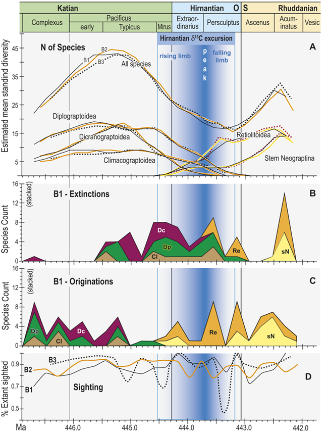
Figure 5 Long description
A. Estimated mean standing diversity in binning schemes B1 to B3 for all graptolite species present through the study interval taken together, alongside those of the three constituent subclades within the Diplograptina: the Dicranograptoidea (D c), Diplograptoidea (D p), and Climacograptoidea (C l), and two subgroups within the Neograptina: stem-group Neograptina (s N) and Retiolitoidea (R e). Variation among results from B1 to B3 is small relative to the large changes in species diversity and to the differences in those changes in diplograptine versus neograptine subclades. Diversity of the diplograptine clade and subclades all peaked during the early part of the Typicus Subchron, irrespective of binning scheme, following which they decline monotonically to final extirpation in the early to mid Persculptus Chron. The Dicranograptoidea increased sharply to a peak of about 19 species in the early part of the study interval and also declined quickly with final extinction at about 444.45 M a whereas the Diplograptoidea (also with about 19 species) and Climacograptoidea (peak diversity: 10 species) declined more slowly with the latter going extinct at about the same time as the Dicranograptoidea and the former persisting to a final extinction late in the Persculptus Chron, at about 444.0 M a. At the same time as the Diplograptina show extended diversity decline, the Neograptina exhibit a steady increase in diversity beginning with their immigration late in the Mirus Subchron synchronously with the early part of the HICE rising limb,
B. Stacked plot of the number of species extinctions within B1 bins by subclade. Species extinctions among the Diplograptina are strongly concentrated in the interval from early Typicus Subchron through the early part of the Extraordinarius Chron, with a second concentration of losses among Climacograptoidea and Diplograptoidea in the mid Persculptus Chron, contemporaneous with the falling limb of the H I C E. There are nearly no extinctions among this clade in the earlier part of the study interval, and species loss among the Neograptina is concentrated in the mid to late Persculptus Chron. A large peak in apparent losses in the Neo clade in the Acuminatus Chron is an artifact of incomplete sampling at the end of the time series.
C. Stacked plot of the number of species originations within B1 bins by subclade. Diplograptine clades show numerous species originations in the Complexus Chron and early in the Pacificus Chron, and none thereafter except for a very few continuing among the Dicranograptoidea into the Mirus Subchron when the Neograptina appear and add many species through the course of the Hirnantian, returning total graptolite diversity to values nearly equal those prior to the mass extinction.
D. Time series of approximate per species sighting probabilities (proportion of observed, extant species recovered in bin) for each binning scheme; values are somewhat variable but are similar among binning schemes, show no long-term trend and values in the mass extinction interval (Mirus plus Hirnantian) are not significantly different from non-extinction interval values; overall the sighting probabilities average 0.88 plusminus 0.22 (95% C I).
The appearance of neograptines during the Mirus Subchron slightly precedes the onset of the HICE in our scaled ordination and manifests as a pulse of species appearances among both the stem-neograptines and the Retiolitoidea within the latest Katian and early Hirnantian. Previous biogeographic analyses suggest that the appearance of Neograptina in the paleotropics at this moment represents an immigration event from mid- to high-latitude regions (Goldman et al. Reference Goldman, Mitchell and Melchin2011). This immigration event coincides in our analyses with the largest number of diplograptine species extinctions recorded during the Late Ordovician (Fig. 5B,C). It is this dramatic disappearance of diplograptine species (and the consequent change in the composition of graptolite and other species assemblages) around the start of the Hirnantian Age that is commonly identified as the first pulse of the LOME. We will return to a discussion of the nature of that event later.
The mean standing diversity values for the graptolite clade as a whole fell to 17.5–15.5 species near the end of the Persculptus Chron; an approximately 62 percent loss of species diversity. The Neograptina diversified during the LOME and became the most specious clade concomitantly with the onset of the postglacial flooding event early in the Persculptus Chron, only some 600 kyr after their initial invasion of the paleotropics. By the early Silurian, in the Acuminatus Chron approximately 1.2 Myr from its nadir, graptolite EMSD had nearly recovered to Katian peak values.
All three of our binning schemes produce essentially the same pattern of change in estimated per capita extinction and origination rates (Fig. 6A,B). Among the Diplograptina rates of origination fall to near zero values by the end of the Typicus Chron while extinction rates slowly rise to a modest peak at the start of the Hirnantian, irrespective of bin boundary placement or whether the bins equalize sampling interval length or the number of horizons in each interval. This general similarity continues through the LOME, with the exception that the very short bin durations in the B3 set through the Katian–Hirnantian transition interval and the postglacial late Persculptus Chron interval produce exceptionally high p̂ values among the Neograptina during both of those intervals (Fig. 6B) as well as an exceptionally high q̂ among the Diplograptina in the late Persculptus Chron (Fig. 6A). The longer durations of the B1 and B2 bins recover similar peaks in the per capita rates but tend to spread them over a broader interval and in some cases shift their timing earlier or later by a half bin. In any case the two clades display strikingly different dynamical histories. This is most notable in the case of the late Persculptus peak rates: Diplograptines experienced high rates of extinction at precisely the same time that Neograptines speciated at high rates.
Time series of per capita and Capture-Mark-Recapture (CMR) model-based estimates of graptolite species turnover dynamics. Species of the clades Diplograptina and Neograptina analyzed separately based on the B1–B3 occurrence records for the per capita rates and the B1 and B2 records for CMR. Timing of neograptine invasion and diplograptine subclade final extinctions shown by arrows along the timeline below A (abbreviations as in Fig. 5). A, Per capita extinction rate (q̂) from B1–B3 data treatments. B, Per capita origination rate (p̂) from B1–B3 data treatments. C, CMR modeled species sighting probabilities (±95 percent bootstrapped CI); sighting rates and CI fixed for both of the highest ranked models of the Diplograptina record and variable for both Neograptina models. D, Extinction rates (±95 percent CI) derived from the highest ranked CMR models; rates time-variant for the Diplograptina in both models and only slightly variable or fixed for the Neograptina. E, Origination rates (±95 percent CI) derived from the highest ranked CMR models; rates fixed or minimally time-variant for the Diplograptina and highly variable for the Neograptina in both models. F, Number of species extinctions in the two clades inferred from the highest ranked B1 and B2 CMR models.
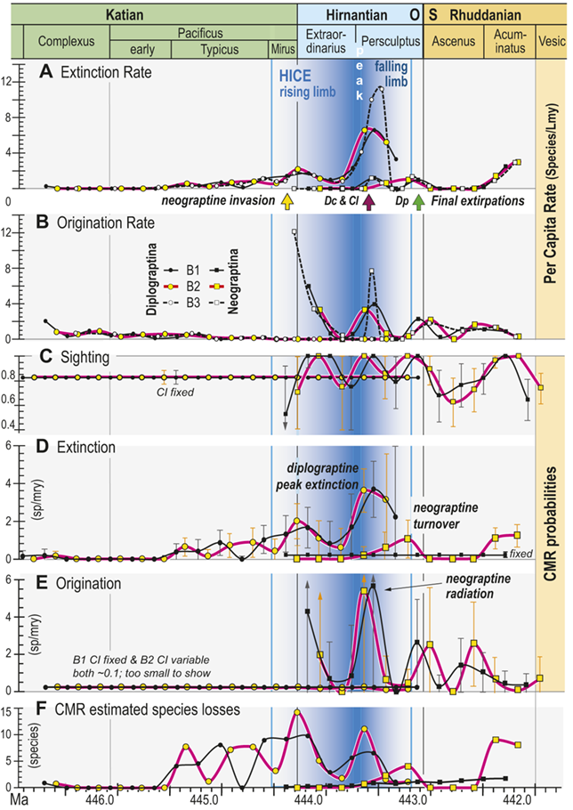
Figure 6 Long description
The values identified in the figure explanation as being plotted in the six panels are all provided in Appendix 2, and the general temporal patterns of species turnover illustrated herein are described in the Results and Discussion portions of the text.
In general, the data plotted in this figure show that extinction risk among the Diplograptina as measured by both approaches and in all three binning schemes was near zero during the Complexus and Lower Subzone intervals and then began a slow climb to moderately a value of about 2 species per m y at the beginning of the Hirnantian, which was followed by a brief decline into the later part of the Extraordinarius Chron before climbing again to a yet higher peak of about 4 s p per m y early in the Persculptus Chron, based on the C M R analyses. The per-capita, face value metrics yield a slightly higher peak of nearly 6 s p per m y at that same point in time. Diplograptines went extinct shortly after that peak, following a partial decline. Taking variation in sighting probability into account, C M R estimates that substantial species losses began abruptly during the Typicus Subchron and grew in number only slightly into the early Hirnantian, but as those losses became a larger fraction of the declining diversity, estimated per-species extinction risk increased. The Neograptina exhibit several peaks in origination and extinction, and these peaks correspond in time with those exhibited by the Diplograptina: the largest neograptine probabilities of origination (greater than 5 s p per m y) occurred in the early Persculptus Chron at the same time as the highest peak in risk of extinction among the Diplograptina.
3.2 Capture-Mark-Recapture Models
We generated CMR models based on the B1 and B2 data treatments for ‘all taxa’ and for the Diplograptina and the Neograptina individually (Table 2). As we noted earlier, the B3 bin set with its unequal interval lengths is not suitable for CMR analysis. Each analysis included a set of models that range from maximally complex models in which all parameters are fully time-variant (pt φt γt) to those that are fully time-invariant (p. φ. γ.) and ranked models according to their AICc weights. The all-taxa models fit parameters to the entire 24-bin time series, whereas those for the two clades employed a shorter time series corresponding to the duration of the clades: bins 1–18 for the Diplograptina and bins 13–24 for the Neograptina. In no case were fully time-invariant models the most highly ranked. For the B1-all taxa models, [p. φt γt] is the highest ranked model with sighting probability treated as fixed (Table 2). The corresponding B2 binning failed to pass the GOF test. The deviance value for the B2 all-taxa dataset was higher than that of 95 percent of the Monte Carlo simulations, indicating that those data are more poorly fit than expected by the most complex (fully time-variant model). As the per capita rates suggest (Fig. 6A,B), the Diplograptina and Neograptina display quite different turnover histories through the Late Ordovician and as a result the combined sighting record of the two clades in the B2 data treatment may not be sufficiently homogenous in its dynamical properties to be fit reliably by standard CMR methods. The best-fit models recovered for the two individual clades varied somewhat depending both on clade and binning. In the case of the Diplograptina, the highest ranked models for both the B1 and B2 data treatments are [p. φt γ.] with fixed rates of sighting and origination (Tables 2, 3). Only extinction rates varied significantly over time in these models of diplograptine turnover. In contrast, the most highly ranked models of the turnover dynamics of the Neograptina were the fully time-variant model [pt φt γt] for the B2 data treatment but, surprisingly, a very low and fixed risk of extinction [pt φ. γt] for the B1 neograptine occurrence record (Table 2). In that model all the variation in species turnover is attributed to a combination of variation in the probabilities of origination and sighting.
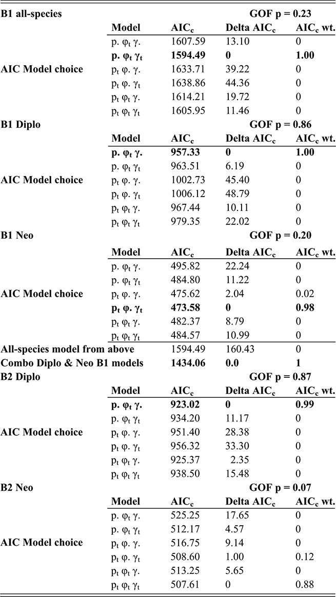
Table 2 Long description
Capture-mark-recapture (C M R) model choice results. This is a complex table arranged into six data blocks. Each block is identified by the data set that was analyzed and presents results for that set. Those results consist of two components: a p-value that expresses the goodness-of-fit between the data set and the C M R model expectations (values greater than 0.95 represent failure to fit). The second component is the main body of each block, and presents the results of comparisons among six alternative models of changing species diversity in the data time series. The models employ three parameters, which are p: prob. of recovery of an extant individual; phi: prob. of individual survival into the following interval; gamma: prob. of seniority (that is, prob. of extant individual having been present in preceding interval). The six alternative models range from one in which only phi varies among time intervals (upper row) to models in which all three parameters are time-variant (lower row). Time-variant parameters are labeled by (t) and those that are invariant by (.). Thus, each row in each data block is a C M R model that is identified by the list of parameters and their temporal variability. The models are compared in the body of each data block on the basis of Akaike’s Information Criterion, modified for low sample sizes (A I C c), as more fully described in the text. Three measures are given for each model, which are, from left to right: A I C c score, delta A I C c (departure of the A I C c score for a particular model from the lowest A I C c score in the set), and finally, relative A I C c weight.
First scenario: B1 All-species data set results goodness-of-fit: 0.23 P. Phi(t) Gamma. 1607.59 13.095 0 P. Phi(t) Gamma(t) 1594.49 0 1.00 P(t) Phi. Gamma. 1633.71 39.215 0 P(t) Phi. Gamma(t) 1638.86 44.364 0 P(t) Phi(t) Gamma. 1614.21 19.723 0 P(t) Phi(t) Gamma(t) 1605.95 11.46 0
For this scenario, the preferred or best-fit model is P. Phi(t) Gamma(t), which has the lowest A I C c score (1594.49), a zero delta A I C c, and the highest relative weight (1.00). Among the analyses of the five principal C M R scenarios, no model with all three parameters fixed or with only the gamma variable was ever among the four highest-ranked models, and so we do not present model choice results for those models in any of the scenarios.
Second scenario: B1-Diplograptina data set results goodness-of-fit: 0.86 P. Phi(t) Gamma. 957.33 0 1.00 P. Phi(t) Gamma(t) 963.51 6.185 0 P(t) Phi. Gamma. 1002.73 45.403 0 P(t) Phi. Gamma(t) 1006.12 48.792 0 P(t) Phi(t) Gamma. 967.44 10.107 0 P(t) Phi(t) Gamma(t) 979.35 22.024 0 Third scenario: B1-Neograptina data set results Goodness-of-fit: 0.20 P. Phi(t) Gamma. 495.82 22.238 0 P. Phi(t) Gamma(t) 484.8 11.218 0 P(t) Phi. Gamma. 475.62 2.037 0.0167 P(t) Phi. Gamma(t) 473.58 0 0.9833 P(t) Phi(t) Gamma. 482.37 8.791 0 P(t) Phi(t) Gamma(t) 484.57 10.985 0 Comparison of the best-fit B1 all-species model to the combined best-fit Diplo and Neo models Best-fit All-species 1594.49 160.43 0 Neo plus Diplo 1434.06 0 1.00 Fourth scenario: B2 Diplograptina data set results Goodness-of-fit: 0.87 P. Phi(t) Gamma. 923.02 0 0.9909 P. Phi(t) Gamma(t) 934.2 11.174 0 P(t) Phi. Gamma. 951.4 28.376 0 P(t) Phi. Gamma(t) 956.32 33.299 0 P(t) Phi(t) Gamma. 925.37 2.347 0.0091 P(t) Phi(t) Gamma(t) 938.5 15.475 0 Fifth scenario: B2 Neograptina data set results Goodness-of-fit: 0.07 P. Phi(t) Gamma. 525.25 17.65 0 P. Phi(t) Gamma(t) 512.17 4.566 0.0001 P(t) Phi. Gamma. 516.75 9.142 0 P(t) Phi. Gamma(t) 508.6 0.996 0.1199 P(t) Phi(t) Gamma. 513.25 5.646 0 P(t) Phi(t) Gamma(t) 507.61 0 0.88
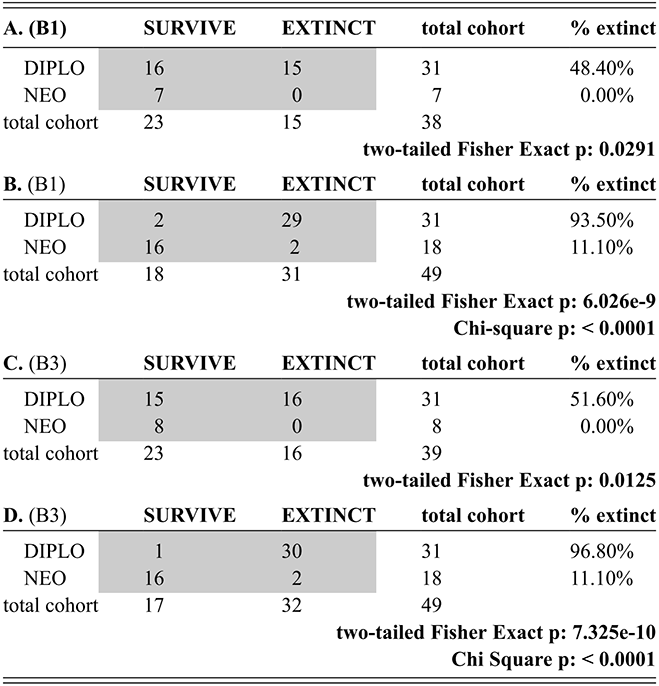
Because the log likelihood values underlying the AIC are additive, it is possible to compare the fit of the B1-all taxa model to a combination of the separate Diplograptina and Neograptina B1 models (Table 2). The combined models yield a substantially lower summed AIC value (reported here following correction to AICc) than that of the highest ranked all-taxon model. Indeed, the resulting deltaAICc is larger than the difference between any of the alternate all-taxa B1 models (Table 2). This result indicates that the dynamical history of graptolites through the LOME is much better fit when the clades are modeled separately. Consequently, we focus for the remainder of the paper on the two-clade CMR models.
The estimated sighting probabilities of ~0.83 for diplograptines leads to higher projected total species diversity in the late Katian (52–58 species) than the estimated diversity obtained via the face-value metrics since in this formalism the observed species diversity is thought to underestimate true standing diversity by 1–p. Additionally, the CMR models suggest a slightly larger, 64–67 percent decline in species diversity during the LOME but recover a similar early Persculptus Chron crossover in the diversity trajectories of the two clades, some 630 Kyr (three bins) prior to the final extirpation of the Diplograptina.
In general, all the per capita rates and CMR estimates of extinction intensity follow comparable trajectories; however, the two prominent peaks in extinction risk present in the face-value rates during the Katian–Hirnantian passage interval (“LOME-1 peak” hereafter) and during the early phase of the falling limb of the HICE (LOME-2 peak) are more subdued in the CMR results. This reflects the fact that the CMR models attribute some of the missing taxa to incomplete sampling rather than to extinction. Consideration of the 95 percent CI bounds on these probabilities reveals two additional salient features. Firstly, the LOME-1 peak was preceded by an interval of elevated extinction risk during the Typicus Subchron that is not significantly lower than that in LOME-1 peak. This extended period of accelerated extinction rates is matched in the CMR results by substantial numbers of implied extinctions through the latest Katian (Fig. 6 F). Secondly, peak values in the LOME-1 were not significantly different than those of the LOME-2 peak, although extinction risk in that interval was significantly elevated relative to that in the Typicus Subchron and relative to the low extinction rates that occurred near the end of the Extraordinarius Chron between these two Hirnantian pulses.
The clade-specific CMR models of species origination reveal a pattern that is less similar to that of the per capita, face-value interpretations in that they estimate a constant low level of origination among the Diplograptina, rather than the modest but declining p̂ shown in the face-value rates, attributing fluctuation in the frequency of species appearances to incomplete sampling (Fig. 6E). Consequently, nearly all variance in occurrences is mapped onto variation in extinction risk (Fig. 6D).
In striking contrast to the diplograptine models, sighting and origination probabilities are strongly time-variant in the CMR models of neograptine turnover (Fig. 6 C,E) and extinction risk is either fixed or only slightly time-variant (Fig. 6D). The 95 percent CI bounds on neograptine extinction risk indicate that the two models differ significantly from one another only in the early Silurian (Fig. 6D), where we suspect that edge-effects (false range truncations) may have contributed to the inferred higher extinction in the B2 set. Origination, on the other hand, reveals two relatively high peaks with similar magnitude and age placement in both binning treatments (differing only in age by the ~ half bin offset). The first of these peaks in origination corresponds to the LOME-2 interval when the Diplograptina experienced the highest levels of extinction risk (Fig. 6D,E). The second represents a third LOME turnover pulse, more or less coincident with the beginning of the Silurian Period, during which the dominance of neograptine clades shifted from retiolitoids to stem-neograptines (Fig. 5B,C) and the final Diplograptina went extinct just prior to the end of the Ordovician (Fig. 6A). Note that during the Hirnantian the origination timeseries for the Neograptina is based on small numbers of species, which leads to high uncertainty in the modeled origination probabilities. The time series is also truncated at its start because we cannot estimate a reasonable value of origination associated with the paleotropical debut of the neograptines during the Mirus Subchron (indicated by a arrow in Fig. 6C) and it is likely that the high origination rate at that point in some measure reflects immigration rather than in situ evolutionary origination of the sighted species. Curiously, the final extirpation of the three diplograptine clades all occurred during intervals of relatively high origination probability among the Neograptina (arrows labeled “Dc & Cl,” and “Dp” in Fig. 6A).
3.3 Species Prevalence
In our examination of the proportion of horizons occupied by extant species within each bin (species prevalence or sp), we utilized the B1 and B3 bin sets. In the former, all bins have a duration of ~210 Kyr and differ from one another in the number of horizons included. In contrast, each of the bins in B3 encompasses 24 horizons but have substantially different durations (Figs. 4, 7B). Despite these differences in approach, the median of the sp values calculated for the diplograptine species during each bin exhibits a significant decline in through the late Katian and Hirnantian for both datasets (B1: r = 0.7118, p = 0.0003; B3: r = 0.7475, p =0.0001). In both sets, median sp reaches a local minimum at the end of the Mirus Subchron (Fig. 7A) and that minimum is followed by a strong rebound in the Extraordinarius Chron, where sp values are comparable to those early in the Pacificus Subchron.
A, Time series of median species prevalence (the fraction of horizons within a bin that include a given species, assessed separately for each species) in the Diplograptina and the Neograptina derived from the contrasting B1 and B3 binning schemes. (B) Time series of the number of horizons per bin for B1 and B3, which have, respectively, intervals with a fixed 210 Kyr duration (B1, equally spaced midpoints) but variable sample sizes versus bins of variable duration (B3, unequally spaced midpoints) but with fixed sample size (24 horizons per interval). (C) Comparison of average species prevalence in diplograptine species during the Katian (ordinate) versus the average species prevalence of the same species during the Hirnantian; Explanation of symbols: (Δ), species with increased prevalence in the Hirnantian; (+), little change in prevalence (less than ±20 percent of Katian average); (•), decreased prevalence. (D) histogram of change in average species prevalence of diplograptine species based on values plotted in C. Values included in red bars (left of the mode) correspond to data plotted in C as (•), modal blue bar as (+) and right-most yellow bar as (Δ).
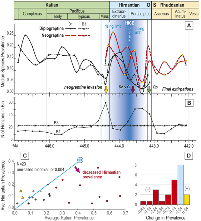
Figure 7 Long description
This complex figure includes four panels. A. The first is a plotted time series of median values of species prevalence. The medians are calculated for all species included in the Diplograptina, and separately for all species in the Neograptina, and thus the plot includes a mean value for each bin for each clade using both the B1 and B3 data sets, which are maximally different in how they combine samples through the time series. Nonetheless, both B1 and B3 time series of median values of species prevalence show very similar trajectories and similar differences between diplograptine and neograptine time series. Although somewhat variable diplograptine median species prevalence values exhibit a significant long-term decline of about 75 percent from initially higher values (approximately 0.2) in the Complexus Chron at the start of the study interval to a minimum (approximately 0.05) during the Mirus Subchron. Those diplograptine values recover to about 0.15 in the mid to late Extraordinarius Chron interval and then again crash to near-zero values as the clade went extinct late in the Persculptus Chron. The timeseries of median species prevalence values for neograptines begins during the Extraordinarius Chron and also shows a peak in values coincident with the resurgent peak exhibited by diplograptines, but with yet higher values (0.20 to 0.25) and then also plummets to a comparable nadir late in the Persculptus Chron, after which it recovers and thereafter fluctuates around a value of 0.12. Thus, both of the intervals of high extinction and origination probability during the L O M E were also intervals of very low median species prevalence.
B. The second panel shows a time series of the number of horizons included in each bin for the B1 and B3 sets. The latter is constant at 24, but the duration of those bins varies widely, with particularly short bins late in the Pacificus Chron and late in the Persculptus Chron, also when median species prevalence was particularly low and extinction risks particularly high. Correspondingly, the B1 bins have relatively high numbers of horizons in those same intervals. Nonetheless, the prevalence values and turnover probabilities of the two binning schemes are essentially the same, indicating that although this increased sampling may affect the dynamical features of the timeseries, they cannot themselves be an artifact of the binnings employed. The text discusses this issue at greater length.
C. The third panel is a scatter plot of species prevalence values for a cohort of 23 diplograptine species that were extant at the peak of diplograptine diversity during the Typicus Subchron. For each species, its average prevalence value during the Katian is plotted along the abscissa versus the average species prevalence value for that same species during the Hirnantian on the ordinate. All but two of those species plot either near a line of slope 1 (indicating no change in average prevalence for those species) or fall to the right of the line (as 13 species do), indicating a decline in species prevalence for those species, in several cases by large amounts. The figure reports that the p value for a one-tailed test of the fit of this outcome to expectations of a binomial distribution is 0.004, which indicates that this outcome is highly unlikely to have arisen by chance: Katian diplograptines that survived into the Hirnantian did so with significantly reduced species prevalence, despite the maintenance of sampling rates in that interval that are comparable to those in the Katian.
D. Final panel displays essentially the same result as a histogram based on the previous cohort of Katian diplograptines, but examining the frequency distribution of differences between the Hirnantian and Katian prevalence values for those species. The histogram shows a mode at the bin that spans zero (minus 0.04 to plus 0.04) and a strongly left-skewed distribution of differences with most contrasts on the negative side of zero and extending out to (minus 0.64 to minus 0.74), but only one bar with two positive contrasts grouped in the zero-adjacent bin (0.04 to 0.14), which distribution then appears very unlike that of a normal binomial distribution, consistent with the test value reported above.
The observed trend in median sp value through the late Katian appears to primarily reflect declining prevalence of individual species rather than a preferential loss of more prevalent species. Twenty-three diplograptine species have multiple occurrences in the late Katian and early Hirnantian in the B-1 bin set. For each of these species, we compared the average sp value among its occurrences in Katian time bins to that for Hirnantian samples and consider any difference less than 0.0± 0.04 (20 percent of the observed standard deviation in the data) to be no change in sp (Fig. 7C,D; this plot is based on B1 data but those from B3 produce equivalent results; given that agreement we did not examine the pattern in B2 data). Under that conservative criterion, prevalence values for only two Katian diplograptines increase in the Hirnantian and seven exhibit no change, whereas sp values for 13 species decreased from the Katian into the Hirnantian. The two-tailed binomial probability associated with this degree of biased outcome is 0.004 (narrower no-change cutoffs of ±0.02 and zero yield outcome ratios of 4:4:15 and 6:0:17, both of which also differ significantly from random expectations). Not surprisingly, species with higher average prevalence during the Katian were more likely to continue into the Hirnantian. We calculated the average species prevalence across all Katian bins for each species present in the cohort of species that was extant at the peak of diplograptine diversity in the Typicus Subchron. We then plotted the age of these species’ last appearance datum (LAD) as a function of their average Katian sp (Fig. 8). Here too the relationship is strongly significant in both the B3 and B1 datasets and is illustrated here for B3. All the species that went extinct during LOME-1 had average sp values in the lower half of the observed range in sp values (< 0.35). Nevertheless, 19 of the 39 species that had average Katian sp values in that same lower half of the range survived into LOME-2 (or, in the case of Paraorthograptus kimi, which is the last known diplograptine, into the late Persculptus Chron LOME-3). That outcome suggests that even species with relatively low species prevalence during the Katian had a 50:50 chance of surviving LOME-1 and remaining among our sampled diplograptine taxa in the Hirnantian.
Correspondence (least squares regression, dashed red line) between the median prevalence of diplograptine species during the Katian and the age of their last appearance datum (bin midpoint) in the B3 dataset (B1 data yield the same result). The plotted species set is the cohort of 46 diplograptine species extant early in the Typicus Subchron (bin 5 of the B3 set), when the Diplograptina reached its peak diversity. The variance explained by the regression (R2) is 0.278 and p, the probability of obtaining this relationship by chance, is 0.0002. Thirty-two species with low species prevalence in this cohort went extinct during LOME 1 (late Katian to earliest Hirnantian) but only seven such cohort members survived into LOME 2 (late Persculptus Chron) whereas all seven species in the cohort that had a species prevalence value in the upper half of the range (>0.32) survived into the later phases of LOME2. Accordingly, it appears that species’ prevalence during the Katian significantly predicts their probability of survival during the LOME.
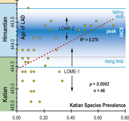
The preceding results could reflect sampling effects. In addition to the general higher rates of loss expected for rare taxa and backwards displacement of their apparent time of extinction (the Signore–Lipps effect, see Wang & Zhong Reference Wang and Zhong2018), sampling effects in this case could also reflect the loss of record caused by facies displacement or omission (e.g., Holland Reference Holland2020, Zimmt et al. Reference Zimmt, Holland, Finnegan and Marshall2021). However, the local nadir in sp values during the Mirus Subchron coincides with an interval of relatively high sampling (large numbers of horizons in each B1 bin and short B3 bins) whereas the peak in median sp values during the Extraordinarius Chron occurs during an interval of lower sampling intensity (Fig. 7A,B). Because most species are uncommon (graptolite species included, Fig. 3; but see also Crampton et al. 2020), as one increases the number of horizons in a sample, the number of sightings for most species increases much more slowly than the number of horizons, which causes the median sp values in the B1 set to exhibit a weak but significant negative correlation with the number of horizons per bin (the slope of the least squares regression is ~0.05 but the 95 percent CI nonetheless excludes zero and the R2 = 0.36 with a two-tailed p = 0.003). The residuals from this regression nonetheless exhibit a minimum in median sp during the same interval as for the original data. Furthermore, the B3 dataset has a constant number of horizons per bin and median sp values in that dataset are not significantly correlated with bin duration or other measures of sampling intensity in our data. Thus, the correspondence in the temporal trajectory of the median sp values in the B3 and B1 indicate that the decline in median sp through the latest Katian reflects a robust pattern of changing species prevalence. Additionally, this result is consistent with the community composition changes assessed from bulk samples at Vinini Creek (Sheets et al. Reference Sheets, Mitchell and Melchin2016), where declining species diversity was accompanied by increased dominance of communities by a smaller number of species. As species diversity declined in this interval, many species were also becoming less common in graptolite collections, and presumably in graptolite communities.
The minimum in median sp during Mirus Chron coincides with the reinvasion of the paleotropics by the neograptines Normalograptus angustus, N. ajjeri, and Metabolograptus ojsuensis. Median sp values for the Neograptina at the time of their debut are higher than those of the contemporaneous Diplograptina. At Vinini Creek neograptine specimens, although representing relatively few species, are by far the most numerous elements of the early Hirnantian faunas (Sheets et al. Reference Sheets, Mitchell and Melchin2016). The relatively high prevalence of neograptines is retained throughout the time series (Fig. 7A) and the two curves largely track one another in both the B1 and B3 sets. Following the recovery in median sp values during the early Hirnantian, values again decline precipitously at the time of the final extirpation of the three diplograptine clades during LOME-2 in the mid to late Persculptus Chron. The late Hirnantian minimum in species prevalence again occurs simultaneously in the B1 and B3 sets and again took place during an interval of relatively high sampling and low origination rates among the neograptines. These relationships suggest that low species prevalence may be causally linked to high extinction risk and reduced probability of origination.
One indication of the nature of that linkage comes from comparison of sp values for individual species with their patterns of specimen abundance in individual bulk samples. Sp values for individual species are significantly correlated with counts of specimen abundance. Sheets et al. (Reference Sheets, Mitchell and Melchin2016) documented shifting patterns of species abundance and community structure at two sites along the Laurentian margin of the Panthalassan Ocean (Vinini Creek and Blackstone River; Fig. 2). Bin-by-bin values of individual species prevalence are significantly correlated with the coeval specimen counts for those same species at Vinini Creek (Fig. 9A) and Blackstone River (Fig. 9B). The relations are illustrated here for B3 but the relationship in data from B1 is similarly significant, despite the considerable scatter in values present. Locally rare species (based on specimen counts) were generally uncommon globally as well, whereas species with locally larger populations tended to have correspondingly higher global prevalence.
Regressions (dashed lines) between number of specimens of individual species in bulk samples (note log scale) and global species prevalence for those same species in coeval temporal intervals. Points labeled by taxon and age but regressions employed all taxa (n is the number of data pairs), with corresponding variance explained (R2) and significance value (p).
species recovered in 16 bulk samples through the Vinini Creek section (mid Complexus to early Persculptus chrons) at Vinini Creek (Sheets et al. Reference Sheets, Mitchell and Melchin2016) versus their coeval species prevalence values in temporal bins B3–2 to B3–16.
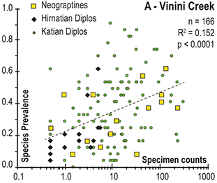
Figure 9(A) Long description
A. Counts of the number of specimens of individual graptolite species recovered in bulk samples from the D. complexus to M. persculptus biozones at Vinini Creek (site 24) are plotted on a log scale along the abscissa versus the species prevalence values for those same species. Species prevalence values are those for the B3 bins in which the Vinini Formation bulk samples were placed in the H A ordination. Thus, individual species may be represented by multiple data points, each corresponding to an age-equivalent pair of bulk samples and a global prevalence value for that species, such that for the Vinini Creek data set, there are 166 data points plotted. Variance explained by linear regression is low (0.152); however, species prevalence is significantly correlated with specimen abundance (p less than 0.0001; analysis with B1 prevalence values produces a similar p value). Data for Katian diplograptine samples and Hirnantian neograptine samples occupy similar regions in the plot; however, those for the Hirnantian occurrences of Diplograptina are clustered in the lower left quadrant of the overall distribution, with low numbers of specimens recovered in the bulk samples and low global species prevalence values. Specimen counts are from Sheets et al. (2016).
, as for A but for bulk samples from Blackstone River (early Pacificus to early Extraordinarius chrons). The prevalence of species is significantly correlated with contemporaneous specimen abundance at each site, suggesting that global prevalence is a function, in part, of specimen density in local populations. Also note that in samples from the Hirnantian strata at Vinini Creek, the carry-over diplograptines generally have lower specimen counts and species prevalence than the diplograptine species did at that site during the Katian and are generally lower in both specimen abundance and species prevalence than the contemporaneous neograptines from that site.
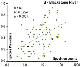
Figure 9(B) Long description
B. Scatter plot like that in A but for specimen counts of species from bulk samples in the upper Katian P. pacificus Biozone to the lower-most beds of the Hirnantian M. extraordinarius Biozone at Blackstone River (Site 4; Sheets et al., 2016) versus the species prevalence values for those species in the B3 bins into which the H A ordination placed those Blackstone River samples, for 82 pairs of values. In this instance, linear regression estimates a slightly higher but still small variance explained (0.224) and a significant correlation between species prevalence and specimen abundance (p less than 0.0001; B1 species prevalence values are similarly well correlated with these specimen abundances). See text for further discussion.
The long-term decline in diplograptine species prevalence and the correlation of species prevalence with specimen abundance, together with the relatively higher species prevalence of contemporaneous neograptine species, accounts for the apparent abruptness of species losses through the Katian–Hirnantian transition at individual sections (Mitchell et al. Reference Mitchell, Sheets and Belscher2007b, Sheets et al. Reference Sheets, Mitchell and Melchin2016). Although precise specimen counts are available only for the Blackstone River and Vinini Creek sections (Sheets et al. Reference Sheets, Mitchell and Melchin2016), qualitative abundance ranks are available for several sections in China (Wangjiawan, the Hirnantian global stratotype section, Honghuayuan, and Fenxiang; Chen Xu et al. Reference Xu, Jia-yu and Mitchell2000, Reference Chen, Jun-xuan, Melchin and Mitchell2005), Dob’s Linn (the Silurian global stratotype section; Williams Reference Williams1982) and Mirny Creek (Koren et al. Reference Koren, Oradovskaya, Pylma, Sobolevskaya and Chugaeva1983). In all these sections, the Diplograptina make up a substantial portion of number of recovered taxa in early Hirnantian assemblages (from a third to as much as 80 percent of the combined diplograptine and neograptine species diversity) but generally are much smaller components when the number of specimens of diplograptines is compared to that of neograptines (Fig. 10). At the intensively collected Mirny Creek section, Parorthograptus sp. occurs as one of only four taxa in the basal Hirnantian strata there but specimens of this graptolite were so few and so poor that T. N. Koren’ was initially reluctant to report it (personal communication, MJM; compare range charts in Koren et al. Reference Koren, Oradovskaya, Pylma, Sobolevskaya and Chugaeva1983, Koren’ & Sobolevskaya Reference Koren’ and Sobolevskaya2008). At each of these sites, diplograptine specimens fall from 100 percent in assemblages during the mid to late Pacificus Chron to generally less than 20 percent (and often much less, especially in more near-shore sites) at the beginning of the Hirnantian and generally continue to decline in abundance through the Hirnantian more rapidly than diplograptine species diversity. Thus, although many diplograptine species survived the transition into the Hirnantian, they appear to have rapidly become minor components of Hirnantian graptolite communities throughout the paleotropics and are correspondingly difficult to recover in graptolite collections. Once again we see here the sort of common cause linkage among specimen abundance, geographic range, stratigraphic duration and ease of collection – between ecology and geology. Notwithstanding that difficulty, it appears that the changes in sp documented earlier likely include a strong signal from changing graptolite metapopulation structures.
Time series of the percentage of faunas within individual Late Ordovician graptolite collections that are comprised by diplograptine species and diplograptine specimens versus the biozonal assignment of those collections. Data from Vinini Creek (site 24), Blackstone River (4), Wangjiawan North (25), Fenxiang (10), Honghuayuan (12), Mirny Creek (19) and Dob’s Linn (6); binned by part of biozone: D. mirus Subzone, and lower, middle, and upper parts of the M. extraordinarius and M. persculptus biozones (see text for references). Late Katian assemblages were dominantly or entirely composed of Diplograptina but as a proportion of graptolite assemblages, the percent of recovered specimens that were diplograptine fell even more precipitously than did the proportion of diplograptine species in those assemblages (gap between average values indicated by stippled area).
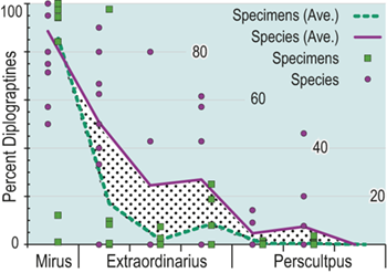
The alteration of graptolite community structure through the LOME is reflected in changing frequency distributions of species prevalence (Fig. 11). The illustrated distributions are derived from the B3 bin set, which once again yields results that are similar to the B1 set but are utilized here because they provide higher resolution through the Katian–Hirnantian transition than the equal duration bin sets. At the peak in graptolite species diversity during the Pacificus Chron (Typicus Subchron) histograms of species prevalence values exhibit the classic strongly right-skewed distribution of species abundance patterns: most species are relatively rare (have low sp values in this context, but as we demonstrated earlier, these values are significantly correlated with local species abundance, site by site), and the frequency of the more abundant species falls approximately exponentially (Fig. 11, Typicus-4–6). However, as species diversity declined through the late Katian, the distribution of species prevalence values contracted leftward and flattened as rare species went extinct and formerly common species became less so, thereby replenishing the low sp tail of the distribution (Fig. 11, Typicus-7–Mirus-9). This latter phase coincided with the interval of increasing extinction risk among the Diplograptina that marks the transition into the LOME-1. Late in the Mirus Subchron the distribution of diplograptine sp values flattened and by the early Extraordinarius Chron the rarest species no longer formed the mode of the distribution. The few surviving diplograptines and the invading Neograptina were unusually prevalent (Fig. 11, Extra-12). The sp distribution recovered somewhat across the Extraordinarius–Persculptus Chron boundary during the interglacial episode between the two principal Hirnantian ice sheet advances (Armstrong & Coe Reference Armstrong and Coe1997, Melchin et al. Reference Melchin, Mitchell, Holmden and Štorch2013, Ghienne et al. Reference Ghienne, Desrochers and Vandenbroucke2014, Mauviel et al. Reference Mauviel, Sinnesael and Desrochers2020), before again flattening during LOME-2.
Interval-by-Interval (or bin-by bin) frequency distributions of individual species prevalence values for species present in each analytical interval (bin) beginning during the Typicus Subchron of the Pacificus Chron, when graptolite species diversity reached its Katian peak (bin B3–4) through the latest Hirnantian Persculptus Chron (B3–19); intervals labeled by chron and bin number. Prevalence values for diplograptines indicated by dark (green) columns and those of neograptines by pale (yellow) columns. Scope of the LOME-1 is indicated by the flattening and leftward shift (toward lower species prevalence, i.e., toward greater rarity) of the frequency distributions, which in the B3 set is exhibited by data from B3–6, late Typicus Chron through B3–12, early in the Extraordinarius Chron. Similar changes occurred during LOME-2 mass extinction phases in the late Persculptus Chron B3–15 and B3–16 intervals. nD and nN indicate the total number of diplograptine and neograptine species in each interval, respectively; NiN: indicates the interval (B3–10 Mirus Chron) during which the Neograptina invaded the paleotropics.
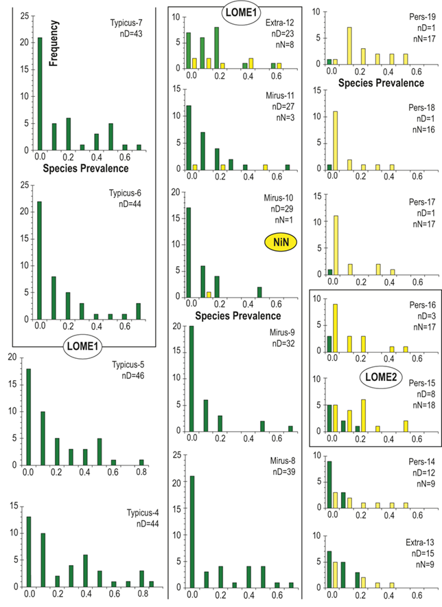
Figure 11 Long description
The 16 histograms included in this figure are all right-skewed, with the mode in the interval of the left-most, and lowest species prevalence (s p) values or one interval farther right at the second lowest values, with a long right-ward tail to s p values greater than 0.6. These distributions are approximately negative log-normal. In the early phases of L O M E 1, the mode grew more populous still, and the columns in the right tail shrank further. Neograptine species entered the assemblages late in the L O M E 1 interval at generally higher s p values, causing a flattening of the histogram distribution in the Extraordinarius Chron as diplograptines with low s p disappeared preferentially (see Figure 8). Although they contain relatively few species, histograms for the latest Extraordinarius B3 to 13 and earliest Persculptus B3 to 14 intervals return to a more nearly log-normal form. In the succeeding L O M E-2, late Persculptus Chron intervals (B3 to 15 and 16), the distributions again flatten and are populated mainly by neograptines. Finally, histograms in the post-L O M E-2 intervals (B3 to 17 to 19) again return to more nearly negative log-normal distributions and include a single diplograptine species (Paraorthograptus kimi) resident in the lowest s p sector of the plots. Species counts in each bin interval shown on the figure are provided in Appendix 2.
Although the changes in sp values described earlier are not primarily artifacts of sampling, it is also not a coincidence that the two intervals of relatively higher sampling (more horizons per unit time) occupy intervals of paleobiological significance (the neograptine invasion and the diplograptine final extirpation). The first encompasses the beginning of the Hirnantian, and graptolite sections around the world have been intensively sampled through that interval with the specific intent to precisely locate species appearances as part of the effort to define the global boundary stratotype of the stage and to better understand the paleobiological events associated with it. The second interval of intense sampling is the interval of postglacial flooding when graptolite-bearing black shales once again became widespread and is followed rapidly by the beginning of the Silurian. These two intervals also correspond to the rising and falling limbs of the HICE and so surely also coincided with substantial changes in the global climate and oceanographic conditions. We turn to a discussion of those events and their relationship to graptolite species turnover in the following section.
4 Discussion
4.1 Timing and Pace of Turnover
The present results indicate that the Late Ordovician change in graptolite species richness and taxonomic composition took place over an extended interval that, at the scale of our analyses, included three distinct turnover phases: first, during the interval of the Katian–Hirnantian boundary, then during the mid Persculptus Chron, postglacial flooding episode, and finally around the beginning of the Silurian (Figs. 5,6, 12; the apparent rise in extinction rate in the Acuminatus Chron is an artifact of range truncation at the end of the sampled time series). Chen Xu et al. (Reference Xu, Melchin, Sheets, Mitchell and Jun-xuan2005b), in their CMR analysis of graptolite turnover record in South China, recovered a similarly extended LOME-1 event as well as a strong turnover pulse near the end of the Hirnantian (LOME-3 as recognized herein). However, the LOME-2 event associated with the end of the postglacial flooding interval was obscured in the relatively poorly fossiliferous facies transition from the Kuanyinchiao lime mudstones (which contain the HICE peak in South China) into the overlying Longmachi black shales and so was expressed mainly as a pulse of neograptine origination and exaggerated extinction in the early Hirnantian. In contrast, analyses of a high-resolution, global composite by Crampton et al. (Reference Crampton, Cooper, Sadler and Foote2016, Reference Crampton, Meyers and Cooper2018)Footnote 2 reveal an overall increased rate of graptolite species turnover during the Hirnantian punctuated by distinct peaks in origination and extinction rates that, as in our results, affect both rates simultaneously. Rather than three Hirnantian turnover peaks, the Crampton et al. results exhibit four, divided in the middle by a sharp decline in rates. We suggest that this lull in species turnover likely corresponds to the pause in turnover captured herein between the extended late Katian to early Hirnantian LOME-1 episode (and corresponding to the first two peaks in the Crampton et al. results) and the pair of intense turnover events (LOME 2 & 3 in our results) that took place during the Persculptus Chron. That interval of reduced turnover appears to correspond to the mid-Hirnantian interglacial (i.e., the interval of sea level rise between LOGC 2 and 3 of Ghienne et al. Reference Ghienne, Desrochers and Vandenbroucke2014; Fig. 1 herein, see also Li Chao et al. Reference Chao, Jun-peng and Wen-jie2021, Jin Si-ding et al. Reference Si-ding, Hai-yang and Ming-cai2024). This interpretation is supported by the spectral analysis of Crampton et al. (Reference Crampton, Meyers and Cooper2018), which those authors concluded reflects orbital forcing of climate change and its effect on graptolite biotopes (see also Cooper & Sadler Reference Cooper and Sadler2010, Cooper et al. Reference Cooper, Sadler, Munnecke and Crampton2014).
Comparison of time series of several measures of graptolite faunal turnover, including the three phases of the LOME described in the text (shaded horizontal bands), to those of estimated sea surface temperature, δ13C, and to the Brenchley et al. (Reference Brenchley, Marshall and Underwood2001) model of graptolite generic turnover through the LOME. (A) δ13C trajectories from Anticosti Island (narrow black curve “A”; from Mauviel & Desrochers (Reference Mauviel and Desrochers2016), Blackstone River (dashed curve “B”; from LaPorte et al., (Reference LaPorte, Holmden and Patterson2009) and Monitor Range (thick blue grey line “M”; from LaPorte et al., (Reference LaPorte, Holmden and Patterson2009) illustrating a range of different trajectories through the Hirnantian carbon isotopic excursion (HICE). (B) Sea surface temperature (SST) with 2σ uncertainty in SST (horizontal error bars) and estimated uncertainty in sample age (vertical error bars); SST data from Finnegan et al. (Reference Finnegan, Bergmann and Eiler2011), but sample ages revised to reflect placement of the beginning of the Hirnantian Stage near the base of the Ellis Bay Formation at Anticosti Island (Achab et al., Reference Achab, Asselin, Desrochers, Riva and Farley2011; Achab et al. Reference Achab, Asselin, Desrochers and Riva2013, Mauviel et al.,Reference Mauviel, Sinnesael and Desrochers2020; Zimmt & Jin, Reference Zimmt and Jin2023; Zimmt et al., Reference Zimmt, Holland, Desrochers, Jones and Finnegan2024) and their correlation to samples in the Cincinnatian succession (Brett et al., Reference Brett, Aucoin and Dattilo2020; Sinnesael et al., Reference Sinnesael, McLaughlin and Desrochers2021). (C) Graptolite species diversity from Fig. 5. (D) Estimated mean standing diversity of graptolite genera (B1 bin set) in the Diplograptina and Neograptina. (E) Capture-Mark-Recapture estimates of species origination and extinction intensity for the Diplograptina and Neograptina, as in Fig. 6D,E. (F) The Brenchley et al. (Reference Brenchley, Marshall and Underwood2001) interpretation of graptolite generic diversity change through the LOME as presented in Harper (Reference Harper2023, Fig. 4), fit to the timing of the HICE.
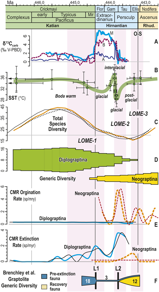
Brenchley et al. (Reference Brenchley, Marshall and Underwood2001) presented a quite different model of the LOME in which essentially the entire graptolite extinction took place in a geologically abrupt event (L1 in Fig. 12G) following which diversity remained low with no new taxa originating prior to the succeeding second pulse (L2) at the end of the Hirnantian glacial epoch. The L1 diversity decline was depicted as occupying a small fraction of the estimated 0.5–1 million years that separated the L1 and L2 events (Brenchley et al. Reference Brenchley, Marshall and Underwood2001, p. 330 and their figure 2). Despite its striking disagreement with a prior quantitative study of graptolite turnover (Melchin & Mitchell Reference Melchin, Mitchell, Barnes and Williams1991) and several subsequent publications (Chen Xu et al. Reference Xu, Melchin, Sheets, Mitchell and Jun-xuan2005b, Fan Jun-xuan & Chen Xu Reference Jun-xuan and Chen2007, Finney et al. Reference Finney, Berry and Cooper2007, Sadler et al. Reference Sadler, Cooper and Melchin2011), this interpretation has been employed explicitly in several recent studies (e.g., Hammarlund et al. Reference Hammarlund, Dahl and Harper2012, Harper et al. Reference Harper, Hammarlund and Rasmussen2014, Bond & Grasby Reference Bond and Grasby2017, Reference Bond and Grasby2020, Harper Reference Harper2023) that relied on geochemical proxies to assess the potential causes of environmental changes during the LOME and implicitly in a large number of others (Bartlett et al. Reference Bartlett, Elrick and Wheeley2018, Zou Cai-neng et al. Reference Cai-neng, Zhen, Heng-ye, Da-zhong and Bin2018b, Li Na et al. Reference Na, Chao and Jun-xuan2019, Hu Dong-ping et al. Reference Dong-ping, Meng-han and Jiu-bin2021, Li Na et al. Reference Na, Chao and Algeo2021, Pohl et al. Reference Pohl, Lu and Lu2021, Jeon et al. Reference Jeon, Li and Kershaw2022, Kozik et al. Reference Kozik, Young and Newby2022b, Liu Mu et al. Reference Mu, Dai-zhao and Lei2022, Qiu Zhen et al. Reference Zhen, Cain-eng and Mills2022, Hu Rui-ning et al. Reference Rui-ning, Jing-qiang and Wen-hui2024, Liang Yu et al. Reference Yu, Zerui Ray and Algeo2024). Indeed, the LOME turnover event does appear as two abrupt extinction-only events, L1 and L2, as depicted in many of the stratigraphic sections examined in these studies. That appearance is largely an artifact, and the causes of the apparent abruptness are several. Holland and Patzkowsky (Reference Holland and Patzkowsky2015), Holland (Reference Holland2020) and Zimmt et al. (Reference Zimmt, Holland, Finnegan and Marshall2021) have described the role of sequence stratigraphic effects on producing apparently pulsed extinction where none existed and we need not repeat that discussion here. We note simply that the ~200 m change in sea level and related facies displacements that were driven by the Hirnantian glaciation clearly fit the conditions under which sequence stratigraphic effects should be pronounced. The extinction pulses that have been identified at the majority of shelf sections, including several of those dominated by graptolite-bearing strata in Laurentia, South China, Chu-Ili Kazakh terrains, and Siberia (see Finney et al. Reference Finney, Berry and Cooper2007), coincide with sharp facies changes and these facies changes clearly have truncated many species ranges in these sections based on our current understanding of their global species ranges (see supplemental data files in Appendix B for range data). These facies and hiatus-related truncations contributed to the apparent abruptness of the LOME species losses in individual sections. Several particular features of graptolite ecology and biogeography also contribute to the apparent abruptness of the LOME turnover. First, diplograptines experienced a dramatic drop in global metapopulation sizes, which is reflected in widespread reduction in the abundance of diplograptine specimens in bedding plane assemblages (Mitchell et al. 2007, Sheets et al. Reference Sheets, Mitchell and Melchin2016) and in their reduced species prevalence (Figs. 7,8,11). Most diplograptines seemed to go extinct in the latest Katian or early Hirnantian when they actually simply became rare (and harder to collect), even in otherwise abundantly graptolitic successions (Fig. 10). Those changes were accompanied by the immigration of several neograptine species that appeared widely in paleotropical assemblages around the globe (high species prevalence) and did so with relatively high specimen abundances (Goldman et al. Reference Goldman, Mitchell and Melchin2011, Sheets et al. Reference Sheets, Mitchell and Melchin2016), which turned most surviving diplograptines into relict species, effectively hidden among the abundant neograptines. This effect is especially strong at sparsely fossiliferous (e.g., Dob’s Linn; Williams Reference Williams1982, Reference Williams1983)Footnote 3 or poorly productive sites (e.g., Mirny Creek; Koren et al. Reference Koren, Oradovskaya, Pylma, Sobolevskaya and Chugaeva1983), but is also evident even in highly productive successions, such as at Vinini Creek, where repeated intensive bulk sampling extended many species ranges compared to those initially reported there (compare Finney et al. Reference Finney, Berry and Cooper2007, Štorch et al. Reference Štorch, Mitchell, Finney and Melchin2011) (see also the discussion in Mitchell et al. Reference Mitchell, Sheets and Belscher2007b, Holland Reference Holland2016, Sheets et al. Reference Sheets, Mitchell and Melchin2016). Thus, the Brenchley et al. model mistakenly accepted the artificially abrupt turnover as an accurate reflection of the extinction dynamics. Recent work suggests that a similar revision of the trajectory of turnover among brachiopods may be necessary as well (e.g., Wang Guang-xu et al. Reference Guang-xu, Ren-bin and Percival2019, Rong Jiayu et al. Reference Jiayu, Harper and Bing2020, Zimmt & Jin Reference Zimmt and Jin2023, Jin & Harper Reference Jin and Harper2024). Whether the same will prove to be true of other clades during the LOME awaits further study.
Although the pace of change during the LOME clearly fluctuated dramatically, the picture that emerges from analyses of graptolite turnover indicates that the entire Late Ordovician glacial interval was a time of ecological and evolutionary flux. Declining species diversity and species prevalence together with rising extinction probability indicate that the LOME-1 events began in the late Katian (Typicus Subchron) as climate transitioned from the Boda warm toward the Hirnantian glaciation (Kröger et al., Reference Kröger, Franeck and Rasmussen2019; Rasmussen et al., Reference Rasmussen, Kröger, Nielsen and Colmenar2019; Fan Jun-xuan et al.,Reference Jun-xuan, Shu-zhong and Erwin2020; Deng Yi-ing et al., Reference Yi-ing, Jun-xuan and Shu-han2021). This phase of the turnover reached a crescendo synchronously with the early Extraordinarius Chron glacial advance and carbon cycle disruptions recorded as the rising limb of the HICE and correlated changes in δ18O due to increased continental ice volume reflected in lower global sea level. Overall the LOME-1 transformation of graptolite faunas encompassed an interval of nearly a million years duration, comparable to the scope of diversity decline and acceleration in extinction rates that affected Late Ordovician biotas more generally (Kröger et al., Reference Kröger, Franeck and Rasmussen2019; Rasmussen et al., Reference Rasmussen, Kröger, Nielsen and Colmenar2019; Fan Jun-xuan et al., Reference Jun-xuan, Shu-zhong and Erwin2020; Deng Yi-ing et al., Reference Yi-ing, Jun-xuan and Shu-han2021). The duration of the LOME-2 and LOME-3 intervals, based on our data, again defined by the timing of final clade extinctions, species prevalence and extinction risk, was of the order of 200 kyr each. LOME-2 spanned the second major glacial advance from the Hirnantian interglacial into the succeeding postglacial sea level rise in the Persculptus Chron. The LOME-2 extinctions also accompanied the maximum extent of the carbon cycle disruption (recorded by the peak HICE excursion) and the interval of its rapid return to conditions more like those of previous epochs (falling limb of the HICE). As we discuss in more detail later, each of these extinction phases also involved new species originations among the Neograptina, again unlike the diversity trajectory depicted in the Brenchley et al. model, which only depicted extinctions (Fig.13C,D,G).
4.2 Selectivity of Turnover
The LOME turnover was highly selective at the clade level. Almost immediately upon discovery of the phylogenetic clade structure of planktic graptolites (Fortey & Cooper Reference Fortey and Cooper1986, Mitchell Reference Mitchell1987, Melchin Reference Melchin1998) it became apparent that the species turnover among graptolites involved a complete replacement of the formerly dominant Ordovician lineages by the greatly diversified descendants of a lineage that includes species of Normalograptus and their descendants (Mitchell, Reference Mitchell, Taylor and Larwood1990; Melchin & Mitchell, Reference Melchin, Mitchell, Barnes and Williams1991; Finney et al., Reference Finney, Berry and Cooper1999; Finney, Reference Finney2001; Chen Xu et al., Reference Xu, Melchin, Sheets, Mitchell and Jun-xuan2005b; Melchin et al., Reference Melchin, Mitchell, Naczk-Cameron, Junxuan and Loxton2011; Sadler et al. Reference Sadler, Cooper and Melchin2011). Survivorship of graptolite species cohorts through the LOME-1 and LOME-2 intervals demonstrate that extinctions throughout the LOME were significantly concentrated among the Diplograptina (Table 3). In contrast to the CMR models for the Neograptina, both of which include high origination rates (Figs. 5B,C), the best-fit CMR models for the Diplograptina posit a very low, albeit nonzero, origination rate (<0.3 sp/myr). Nevertheless, all known species originations during the Hirnantian occurred among the Neograptina, which (allowing for range uncertainty) added 16–19 species during the Hirnantian.
Unlike the LOME-1 and LOME-2 events, the LOME-3 episode affected only the Neograptina. By that point the Diplograptina were all but gone. Nonetheless, this event too, exhibited a substantial degree of selectivity. The initial radiation of neograptines in the early Hirnantian took place almost exclusively among the neodiplograptines (a paraphyletic stem group within the Retiolitoidea) and LOME-3 extinction occurred primarily among species of this clade whereas the stem-neograptines (which includes the conservative Normalograptus species) did not diversify until the postglacial Hirnantian (late Persculptus Chron) and early Silurian, when they gave rise to morphologically innovative dimorphograptids and monograptids (Fig. 5; Melchin et al. Reference Melchin, Mitchell, Naczk-Cameron, Junxuan and Loxton2011, Bapst et al. Reference Bapst, Bullock, Melchin, Sheets and Mitchell2012).
4.3 Simultaneous Origination and Extinction
The driving forces behind the LOME produced a positive correlation between origination and extinction throughout the mass extinction interval. Peaks in neograptine origination coincided with peaks in diplograptine extinction during both LOME-1 and LOME-2, each separated by an interval of low turnover near the end of the Extraordinarius Chron (Fig. 12E). Following their immigration from the cool-temperate zone into low-latitude regions at the outset of the LOME-1 (Goldman et al. Reference Goldman, Mitchell and Melchin2011, Goldman et al. Reference Goldman, Maletz, Melchin, Jun-xuan, Harper and Servais2014), neograptine species richness (Fig. 5A), genus richness (Fig. 12D) and, to a lesser degree, structural diversity (Melchin et al. Reference Melchin, Mitchell, Naczk-Cameron, Junxuan and Loxton2011, Bapst et al. Reference Bapst, Bullock, Melchin, Sheets and Mitchell2012) expanded monotonically throughout the interval of the LOME. Thus, rather than being broadly detrimental for the pelagic biota (as one might expect for widespread oceanic anoxia, for instance), conditions during the LOME not only selectively favored the Neograptina, they did so contemporaneously (at least at the 210 kyr temporal scale of our dataset) with the negative effects that drove the Diplograptina to total extinction. In contrast, by the LOME-3 interval, diplograptines were all but extinct and the correlated peaks in origination and extinction in that episode almost exclusively arise from neograptine turnover.
4.4 Metapopulation Dynamics
The LOME turnover was accompanied by increasing rarity of diplograptine species. Diplograptines experienced significant reduction in species prevalence through the latest Katian and early Hirnantian (Figs. 7A,11) as well as a greatly diminished specimen abundance among the species that survived into the Hirnantian (Figs. 9,10). The result was that populations of most surviving diplograptines in the Hirnantian seldom reached local population sizes that were large enough to allow them to be routinely present in fossil collections. This suggests that diplograptine species occupied smaller geographic ranges and had more sparse populations, creating overall decreased total metapopulation sizes with lower spatial persistence. These changes in metapopulation dynamics exposed species to increased risk of extinction (Fig. 8). The immigrant neograptines replaced diplograptines during the earliest Hirnantian as the most widespread and abundant graptolite species. Furthermore, neograptines in general retained greater species prevalence and specimen abundance throughout the Hirnantian, regardless of the rise and fall of species prevalence in the two clades during the LOME (Figs. 7,9). This pattern of diminished diplograptine metapopulations is evident in well-studied paleotropical sites from around the globe; that is, from sections in South China (Wangjiawan-North, Hongjuayuan and Fenxiang; Chen Xu et al. Reference Xu, Jia-yu and Mitchell2000), western Laurentia (Vinini Creek and Blackstone River; Sheets et al. Reference Sheets, Mitchell and Melchin2016) and Kolyma-Omolon (Mirny Creek; Koren et al. Reference Koren, Oradovskaya, Pylma, Sobolevskaya and Chugaeva1983), which together span ~ 210° in longitude around the paleotropics (Figs. 1, 2, 10).
4.5 Relationship to Changing Phytoplankton Communities
Drawing upon new and previously published N isotopic data, Melchin et al. (Reference Melchin, Mitchell, Holmden and Štorch2013) argued that graptolite mass extinction during the LOME was strongly linked to changes in Late Ordovician phytoplankton communities. Evidence in support of this idea has continued to grow. The δ15N of organic matter preserved in sediments deposited in the late Katian during the greenhouse conditions of the Boda interval immediately prior to the onset of the LOME generally have near zero values (±0.5 ‰). These low levels of 15N-enrichment have been widely interpreted to be the result of nearly complete remineralization of fixed N by denitrification within the deep ocean in layers of persistently deoxygenated seawater, or in oxygen-depleted zones within areas of upwelling near the continental margins (LaPorte et al. Reference LaPorte, Holmden and Patterson2009, Melchin et al. Reference Melchin, Mitchell, Holmden and Štorch2013, Luo Gen-ming et al. Reference Gen-ming, Algeo and Ren-bin2016, Liu Yu et al. Reference Liu, Chao, Jun-xuan and Algeo2020, Yang Xiang-rong et al. Reference Xiang-rong, De-tian and Tong2020, Yang Sheng-chao et al. Reference Chao, Jun-peng and Wen-jie2021, Yang Xiang-rong et al. Reference Xiang-rong, De-tian and Dai-zhao2021). That interpretation suggests that photosynthesis in the relatively oligotrophic overlying water mass likely was dependent on biological fixation of N by cyanobacteria. This inference is supported by the fact that lipid biomarker suites from Boda interval samples are dominated by hopanes, consistent with those of cyanobacteria as well as 3β-methylhopanes (3-MeH) characteristic of methanotrophic proteobacteria (Rohrssen et al. Reference Rohrssen, Love, Fischer, Finnegan and Fike2013, Hu Rui-ning et al. Reference Rui-ning, Jing-qiang and Wen-hui2024, Liang Yu et al. Reference Yu, Zerui Ray and Algeo2024). Considering the widespread occurrence of paleotropical diplograptines in sediments of that character, it is reasonable to suppose that these graptolites relied upon some combination of cyanobacteria and the chemosynthetic or heterotrophic microflora (including methanotrophic proteobacteria) of a tropical denitrification zone composed of oligotrophic shallow waters overlying expansive layers of anoxic deep waters (Finney et al. Reference Finney, Berry and Cooper2007, Cooper et al. Reference Cooper, Rigby, Loydell and Bates2012). In contrast, during the LOME interval, N isotopic data from low- latitude settings in Laurentia and South China suggest less intense denitrification concomitantly with an increase in sterane concentrations and other biomarkers consistent with green algal productivity as well as a reduction in the concentrations of 3-MeH, an indicator of methanotrophy (Rohrssen et al. Reference Rohrssen, Love, Fischer, Finnegan and Fike2013, Luo Gen-ming et al. Reference Gen-ming, Huan, Algeo, Hallmann and Shu-cheng2018, Hu Rui-ning et al. Reference Rui-ning, Jing-qiang and Wen-hui2024). These changes suggest that the deep waters of the oceans were more oxygenated during the glaciations, consistent with the reduction in methanotrophy and water column denitrification, and overall increased productivity among eukaryotic algal phytoplankton (Rohrssen et al. Reference Rohrssen, Love, Fischer, Finnegan and Fike2013, Shen Jia-heng et al. Reference Jia-heng, Pearson and Henkes2018, Hu Rui-ning et al. Reference Rui-ning, Jing-qiang and Wen-hui2024) due to the increased availability of recycled sources of fixed-N (LaPorte et al., Reference LaPorte, Holmden and Patterson2009). The LOME-1 and LOME-2 intervals also included accelerated turnover in the fossil record of phytoplankton taxa in the paleotropics (Delabroye et al. Reference Delabroye, Munnecke and Vecoli2011).
In this context it is worth recalling that eukaryotic algal cells are roughly an order of magnitude larger than bacterial cells, which are so small that molecular motion in sea water prevents individual cells from sinking. Shen et al. (Reference Jia-heng, Pearson and Henkes2018)Footnote 4 argued that the increased productivity by algae during the late Katian and Hirnantian may have increased rates of carbon burial and, in turn, contributed to the C-cycle changes recorded in the HICE (we return to that topic later). Our point here is that this change to more abundant, larger phytoplankton is also likely to have negatively affected the food supply of paleotropical diplograptines.
Coeval strata from the cool-temperate Late Ordovician succession in the Prague synform (then part of the peri-Gondwanan microcontinent of Perunica) do not show a significant shift in δ15N through the LOME interval, consistent with the relatively shallower, oxygenated and well-mixed water column in that region (Melchin et al. Reference Melchin, Mitchell, Holmden and Štorch2013). Under these conditions the Late Ordovician phytoplankton community in temperate and higher-latitude sites likely included a relatively high contribution from green algae compared to cyanobacteria and methanotrophs. Perhaps not coincidentally, all of the neograptine species known to have migrated into the paleotropics during the onset of the LOME-1 (Normalograptus angustus, N. ajjeri, Neodiplograptus charis and Metabolograptus ojsuensis) also occur in the Katian–Hirnantian succession in Perunica (Kraft et al. Reference Kraft, Štorch and Mitchell2015, CEM unpublished), Iberia (Mitchell et al. Reference Mitchell, Štorch, Holmden, Melchin, Gutierrez-Marco, Gutierrez-Marco, Rábano and García-Bellido2011) and North Africa (Denis et al. Reference Denis, Buoncristiani, Konaté, Ghienne and Guiraud2007). Thus, the character of the phytoplankton community in low-latitude oceanic settings during the Hirnantian glaciation likely shifted away from the particular conditions to which the Diplograptina had adapted during the Boda interval and toward compositions more similar to those at higher latitudes; that is, toward conditions to which the Neograptina were already adapted.
These inferences are also consistent with those of Crampton et al. (Reference Crampton, Meyers and Cooper2018). Their spectral analysis of a timescaled 64 Myr-long composite of graptolite species ranges (see also Footnote 2) revealed highly significant periodicities of 1.3 and 2.6 my duration in the probability of both extinction and origination. Based on comparison to the Earth’s orbital periodicity during the Cenozoic, Crampton et al. concluded that these periods likely corresponded to Milankovitch “grand cycles” in obliquity and eccentricity, respectively. “These grand cycles would have modulated climate variability, alternating times of relative stability in the environment with times of maximum volatility, which influenced oceanic circulation and structure and thus, phytoplankton populations at the base of the marine food web (Crampton et al. Reference Crampton, Meyers and Cooper2018, p. 5686; emphasis added),” in agreement with the earlier studies of LaPorte et al. (Reference LaPorte, Holmden and Patterson2009) and Melchin et al. (Reference Melchin, Mitchell, Holmden and Štorch2013). We return to the connection between graptolite turnover and climate cycles in the following section.
4.6 Relationship to C-Cycle and Anoxia
Considerable evidence indicates that anoxic to euxinic conditions were widespread during the latest Katian to Rhuddanian interval (e.g., Dahl et al. Reference Dahl, Hammarlund, Rasmussen, Bond and Canfield2021, Li Na et al. Reference Na, Chao and Algeo2021, Pohl et al. Reference Pohl, Lu and Lu2021, Kozik et al. Reference Kozik, Gill, Owens, Lyons and Young2022a, Song Li-cai et al. Reference Li-cai, Qing, Hui-jun and Chang-zhou2023, Yang Sheng-chao & Fan Jun-xuan Reference Sheng-chao and Jun-xuan2025). Furthermore, several studies have argued from those data that the LOME extinction event resulted in whole or in part from the direct kill effects of anoxia itself or from sulfide or toxic metal poisoning, or some combination of these redox-related effects (e.g., Hammarlund et al. Reference Hammarlund, Dahl and Harper2012, Vandenbroucke et al. Reference Vandenbroucke, Emsbo and Munnecke2015, Bartlett et al. Reference Bartlett, Elrick and Wheeley2018, Zou Cai-neng et al. Reference Cai-neng, Zhen and Poulton2018a, Bond & Grasby Reference Bond and Grasby2020, Dahl et al. Reference Dahl, Hammarlund, Rasmussen, Bond and Canfield2021). Given that the case for anoxia as a driver of mass extinction hinges critically on the coincidence in time and space between anoxia and the extinction of the organisms it is alleged to have affected, we begin our consideration of the question of whether widespread anoxia may account for the timing and selectivity of the LOME turnover among graptolites with a brief synthesis of the temporal and spatial distribution of anoxia through the Late Ordovician and early Silurian.
The consensus of the available evidence suggests that ocean oxygenation through the latest Ordovician and early Silurian falls into three distinct phases. 1. late Katian (Pacificus Chron): anoxia was widespread, ranging from locally intermittent to persistent (Fig. 13; Melchin et al. Reference Melchin, Mitchell, Holmden and Štorch2013, Kozik et al. Reference Kozik, Young and Newby2022b, Liu Mu et al. Reference Mu, Dai-zhao and Lei2022, Song Li-cai et al. Reference Li-cai, Qing, Hui-jun and Chang-zhou2023). 2. Hirnantian Glaciation (Extraordinarius – early Persculptus chrons): in this interval anoxia was generally less persistent and more localized except during a brief period of sea level rise associated with the mid-Hirnantian interglacial warm period that separated the two main cycles of ice-sheet advance recorded in North Africa. The interglacial lies stratigraphically just below the main peak of the HICE around the globe, including several sections in South China (Li Chao et al. Reference Chao, Jun-peng and Wen-jie2021, Li Na et al. Reference Na, Chao and Algeo2021, Chen Qing et al. Reference Qing, Ji-tao, Wen-jie and Zhen-sheng2023), western Laurentia at the Vinini Creek, Blackstone River, and Monitor Range sections, (lower Persculptus Biozone, O5c max deepening; Fig. 1; Holmden et al. Reference Holmden, Mitchell and LaPorte2013, Sheets et al. Reference Sheets, Mitchell and Melchin2016, Ahm et al. Reference Ahm, Bjerrum and Hammarlund2017) and eastern Laurentia on Anticosti Island (in the Lousy Cove Member of the Ellis Bay, with an occurrence of Metabolograptus parvulus and geochemical proxies suggesting global anoxia (Melchin Reference Melchin2008, Bartlett et al. Reference Bartlett, Elrick and Wheeley2018, Kozik et al. Reference Kozik, Gill, Owens, Lyons and Young2022a), and at Dob’s Linn (the Extraordinarius Band, Fig. 1; Melchin et al. Reference Melchin, Holmden, Williams, Albanesi, Beresi and Peralta2003, Bond & Grasby Reference Bond and Grasby2020, Mitchell & Melchin Reference Mitchell and Melchin2020), among other sites. 3. Late Hirnantian to Rhuddanian: anoxia became widespread again with the deglaciation of Gondwana and rapid sealevel rise, as indicated by profound shifts in geochemical redox proxies (e.g., Smolarek et al. Reference Smolarek, Marynowski, Trela, Kujawski and Simoneit2017, Young et al. Reference Young, Benayoun and Kozik2020, Dahl et al. Reference Dahl, Hammarlund, Rasmussen, Bond and Canfield2021, Li Na et al. Reference Na, Chao and Algeo2021) and by the global distribution of black shales with high TOC contents in deep shelf to basinal facies (e.g., Melchin et al. Reference Melchin, Mitchell, Holmden and Štorch2013, Yang Sheng-chao & Fan Jun-xuan Reference Sheng-chao and Jun-xuan2025, and references therein). Melchin et al. recognized this particularly widespread interval of anoxia and high-TOC-bearing “hot” shales as the “Rhuddanian Oceanic Anoxia Event” (Rhuddanian OAE). The great preponderance of volcanic ash deposits (summarized in Longman et al. Reference Longman, Mills, Manners, Gernon and Palmer2021) and Hg anomalies (Jones et al. Reference Jones, Martini, Fike and Kaiho2017, Smolarek-Lach et al. Reference Smolarek-Lach, Marynowski, Trela and Wignall2019, Hu Dong-ping et al. Reference Dong-ping, Meng-han and Jiu-bin2021, Song Li-cai et al. Reference Li-cai, Qing, Hui-jun and Chang-zhou2023) that have been cited as evidence of voluminous volcanic activity in the late Katian to early Rhuddanian rocks occurs within the first and third of the three axoxia-rich intervals just outlined here. On the other hand, several studies have suggested that few of the reported Hg enrichments in this interval are volcanic in origin (Shen Jun et al. Reference Jun, Algeo and Jiu-bin2019, Shen Jun et al. Reference Jun, Algeo and Qing-lai2022, Zhou Yu-ping et al. Reference Yu-ping, Yong and Wang2024) and thus it remains unclear to what degree volcanic activity may have contributed to the widespread development of anoxia during the Rhuddanian OAE.
Does the pattern of graptolite turnover during the LOME conform with the timing and expected effects of widespread, shallow oceanic anoxia? We believe it does not. It is conceivable that reduction in population size and fission of species ranges might well accompany increased oceanic anoxia or upwelling of sulfidic water masses and that these changes might increase the risk of extinction and the likelihood of species vicariance, and thus contribute to the linked extinction and origination observed among graptolites. The timing of widespread anoxia fits poorly to the timing of LOME-1 graptolite species losses, however. Firstly, diplograptines were at their peak diversity during the time of widespread Pacificus Chron anoxia; secondly, the rise in rates of extinction and falling origination among these species preceded and persisted longer than the pulse of anoxia locally present at the Katian–Hirnantian boundary; and thirdly, the highest rates of graptolite species extinction during LOME-1 occurred in the early Hirnantian when the oceans were less anoxic than previously. In contrast, the timing of anoxia during the late Hirnantian–early Rhuddanian postglacial interval (Rhuddanian OAE) does correspond well to those of LOME-2 and LOME-3 episodes, during which the few remaining diplograptines and numerous neograptines went extinct. We note that our results indicate that the duration of the species turnover during the Rhuddanian OAE was much more extended than the concentrated episode that is typically shown for LOME-2. Furthermore, the Rhuddanian OAE coincides with a marked diversification (both in taxa and in colony structure) among the Neograptina; an expansion that continued through the entire Rhuddanian Age (e.g., Melchin et al. Reference Melchin, Mitchell, Naczk-Cameron, Junxuan and Loxton2011, Sadler et al. Reference Sadler, Cooper and Melchin2011, Deng Yi-ing et al. Reference Yi-ing, Jun-xuan and Shu-han2021, Štorch Reference Štorch2023). Based on our understanding of the paleoecology of graptolites (see Cooper et al. Reference Cooper, Rigby, Loydell and Bates2012), however, we can envision no reasonable scenario in which these physical drivers could cause extinction to be limited almost exclusively to the Diplograptina and origination to occur only, and simultaneously, in the Neograptina, as evidently was the case, nor to produce the different turnover histories exhibited by the two main neograptine clades (stem-neograptines and the Neodiplograptidae).
It is important to keep in mind that diplograptine and neograptine species occur together in the great preponderance of latest Katian and early Hirnantian samples and so they must have occupied more or less the same sites and water masses most of that time. The same is also true of the two neograptine groups, species of which occur side by side in Hirnantian samples all across the paleotropics. Additionally, although the neograptines for which Sheets et al. (Reference Sheets, Mitchell and Melchin2016) inferred biotope affinities were all identified as epipelagic species, so too were the majority of the diplograptines and both they and the deeper-water, mesopelagic diplograptines ultimately all went extinct, in spite of the differences in their biotope affiliation and the initially higher rates of loss among the mesopelagic species. Thus, although a depth-stratified model of risk in which deeper-dwelling species were more affected by anoxia than the epipelagic species could account for the preferential species losses among mesopelagic species (see also Li Na et al. Reference Na, Chao and Algeo2021), it fails to account for the overall joint pattern of graptolite origination and extinction.
An alternative explanation for the initially higher rate of extinction of mesopelagic species may lie in their resource utilization and likely smaller geographical ranges. In their study of the influence of biotope on extinction risk among Ordovician graptolites, Cooper and Sadler (Reference Cooper and Sadler2010) found that mesopelagic species had significantly and consistently higher rates of extinction. Since graptolites were most abundant and diverse around the margins of continental shelves (like microzooplankton today and oceanic productivity more generally), Cooper and Sadler reasoned that, other things being equal, species confined to deeper shelf-edge habitats likely had smaller geographic ranges (and so, overall smaller metapopulation sizes). They also noted that these more limited habitats likely were more sensitive to climate disruption. Boyle et al. (Reference Boyle, Sheets and Wu2017) also found that off-shore obligate graptolite species also had significantly higher extinction risk than did species that displayed no facies-limited occurrences but found that overall commonness (the combination of number of occurrences and geographic range), which again is likely to be related to total metapopulation size, provided the strongest explanation for variation in species extinction risk. Those inferences have received support from subsequent work that shows graptolite species turnover to be closely correlated with climate fluctuation and the related habitat disruptions (Cooper et al. Reference Cooper, Sadler, Munnecke and Crampton2014, Crampton et al. Reference Crampton, Cooper, Sadler and Foote2016, Reference Crampton, Meyers and Cooper2018). These features naturally would result in an earlier and more intense response among mesopelagic species, as a group, to the climate disruptions that accompanied the Hirnantian glaciation than the, on average, more widely distributed epipelagic species, consistent with the findings of Sheets et al. (Reference Sheets, Mitchell and Melchin2016) and Li Na et al. (Reference Na, Chao and Algeo2021).
Rather than direct kill effects, it appears that the principal importance of anoxia during the LOME interval is that it attests to the disruptions experienced by the oceanic ecosystem. Anoxia in this interval has been widely attributed to high rates of organic matter (OM) productivity and, together with the HICE, has been taken to record an interval of relatively high rates of OM burial relative to inorganic C sequestration rates (e.g., Marshall & Middleton Reference Marshall and Middleton1990, Saltzman Reference Saltzman2005, Qiu Zhen et al. Reference Zhen, Cain-eng and Mills2022, Algeo & Shen Jun 2023, Young et al. Reference Young, Edwards, Ainsaar, Lindskog and Saltzman2023, Liang Yu et al. Reference Yu, Zerui Ray and Algeo2024). Several lines of evidence suggest that the surface waters of the oceans during the LOME-1 interval experienced an increase in nutrient supply (fixed nitrogen and P, among others) through invigorated upwelling (LaPorte et al., Reference LaPorte, Holmden and Patterson2009;Melchin et al., Reference Melchin, Mitchell, Holmden and Štorch2013; Luo Gen-ming et al., Reference Gen-ming, Algeo and Ren-bin2016; Liu Yu et al., Reference Liu, Chao, Jun-xuan and Algeo2020; Yang Sheng-chao et al., Reference Chao, Jun-peng and Wen-jie2021; Zan Bo-wen et al., Reference Bo-wen, Chuan-long and Lash2024), higher volcanic weathering inputs (Yang Sheng-chao et al., Reference Sheng-chao, Wen-xuan and Xiao-lin2019; Longman et al., Reference Longman, Mills, Manners, Gernon and Palmer2021) and increased terrestrial runoff more generally (Lenton et al., Reference Lenton, Dahl and Daines2016; Porada et al., Reference Porada, Lenton and Pohl2016; Dahl & Arens, Reference Dahl and Arens2020; Müller et al. Reference Müller, Joachimski, Lehnert, Männik and Sun2024). Ventilation of the deep ocean reduced the distribution of anoxic marine sediments and the associated burial of OC in sediments underlying anoxic marine bottom waters. To offset the reduction in anoxic marine facies, OC burial would need to have increased in oxygenated marine sediments to account for the HICE. Such an increase in OC burial could have been a result of the increased abundance of larger and more decay-resistant particles contributed from nonvascular land plants and eukaryotic algae (Lenton et al., Reference Lenton, Crouch, Johnson, Pires and Dolan2012; Parnell & Foster Reference Parnell and Foster2012; Rohrssen et al., Reference Rohrssen, Love, Fischer, Finnegan and Fike2013; Lenton et al., Reference Lenton, Dahl and Daines2016; Shen Jia-heng et al., Reference Jia-heng, Pearson and Henkes2018; Hu Rui-ning et al., Reference Rui-ning, Jing-qiang and Wen-hui2024), or by overall slower organic matter decomposition rates in the colder Hirnantian oceans (Stanley, Reference Stanley2010; Finnegan et al., Reference Finnegan, Fike, Jones and Fischer2012a). Melchin et al., (Reference Melchin, Mitchell, Holmden and Štorch2013) noted, however, that there is no direct evidence of increased sedimentary carbon storage during the early mid Hirnantian: nearly all rocks of that age have lower concentrations of organic matter than those before and after the HICE rather than the predicted increases (see also Yang Sheng-chao & Fan Jun-xuan, Reference Sheng-chao and Jun-xuan2025). Arguments that the missing carbon-rich sediments were largely confined to sediments deposited in the abyssal depths and subsequently subducted with the oceanic sea floor or destroyed by tectonic forces, although possible, seem forced at best considering that most oceanic productivity occurs near continental margins, and that bottom-water anoxia was more widespread before and after the main glacial epoch when sedimentary TOC contents were higher and δ13C values were lower than in sediments deposited during the HICE. Furthermore, it is not clear how widespread anoxia in the abyssal realm could account for the LOME in any case. The observed diversity changes that constitute the LOME are virtually all based on the fossil record of organisms that lived on the continental shelves and in epicontinental seas rather than in the abyssal ocean floor, which has an extremely limited fossil record during the Paleozoic Era. Accordingly, it appears unlikely that the positive δ13C excursion can be attributed to increased productivity or its burial efficiency (Olivarez Lyle & Lyle, Reference Olivarez Lyle and Lyle2006).
An alternative resolution to this apparent conflict may be found among the other factors that influence the δ13C value of ocean C reservoir, such as the globally averaged δ13C value of the weathered carbon flux from the continents, and the photosynthetic fractionation factor (εP) associated with marine primary production. Kump et al. (Reference Kump, Arthur and Patzkowsky1999) and Kump and Arthur (Reference Kump and Arthur1999) employed a simple box model to explore the implications of global changes in these parameters as an alternative means of forcing the HICE without increasing the fraction of organic carbon relative to inorganic carbon buried in marine sediments. Increasing the δ13C value of weathered C flux to the oceans by 4‰ and εP by 7‰ (≡ Δ13C = δ13Ccarb – δ13Corg) could account for the magnitude of the largest reported C isotopic excursion (CIE) of 7‰, which they (and many others since, e.g., Brenchley et al., Reference Brenchley, Carden and Hints2003; Bergström et al., Reference Bergström, Chen, Gutiérrez-Marco and Dronov2009; Lenton et al., Reference Lenton, Dahl and Daines2016; Algeo & Shen Jun, Reference Algeo and Jun2023; Zhang Jun-peng et al., Reference Jun-peng, Chao and Yang-yang2024) assumed represented the global shift in the δ13C values of the ocean and atmosphere during the glaciation. Subsequently, shelf gradients in the magnitude of the HICE were found by Melchin and Holmden (Reference Melchin and Holmden2006) and LaPorte et al. (Reference LaPorte, Holmden and Patterson2009): shallow nearshore environments generally record larger excursions than deeper offshore ones (see also Jones et al., Reference Jones, Brothers and Crüger Ahm2020). CIEs in offshore settings average just 2.7 ± 0.4‰ (LaPorte et al., Reference LaPorte, Holmden and Patterson2009), or 1.5‰ if only the deepest setting is considered (LaPorte et al., Reference LaPorte, Holmden and Patterson2009; Ahm et al., Reference Ahm, Bjerrum and Hammarlund2017). These offshore sites are more likely than nearshore settings to record the true change in ocean C cycling during the glaciation. Additionally, many Yangtze Platform sections yield similarly low-amplitude HICE excursions (e.g., Gorjan et al., Reference Gorjan, Kaiho, Fike and Chen2012; Yan De-tain et al., Reference De-tain, Hua and Qi-long2015; Zou Cai-neng et al., Reference Cai-neng, Zhen and Poulton2018a; Song Li-cai et al., Reference Li-cai, Qing, Hui-jun and Chang-zhou2023; Yang Sheng-chao et al., Reference Sheng-chao, Jun-xuan and Algeo2024). Because the magnitude of the excursion in δ13C is smaller than previously thought, the sea level–driven perturbation in carbonate weathering is by itself more than enough to account for the positive excursion. The 7‰ additional increase in globally averaged εP (Kump et al., Reference Kump, Arthur and Patzkowsky1999), which subsequent studies failed to corroborate (Melchin & Holmden, Reference Melchin and Holmden2006; LaPorte et al., Reference LaPorte, Holmden and Patterson2009); is not needed. Using the same model setup and C-cycle parameters as Kump et al. (Reference Kump, Arthur and Patzkowsky1999), a 6 percent increase in carbonate weathering predicts a CIE of 1.5‰. If we instead use the full 22 percent increase in carbonate exposure inferred from geological maps, then the same 1.5‰ excursion can be achieved with a co-occurring decrease of 6 percent in the fraction of organic carbon buried relative to inorganic carbon buried in marine sediments (Table 4). In this scenario, the δ13C value of the riverine flux of dissolved C to the oceans changes from –7 to –5‰ representing contributions from carbonate weathering (80 percent at 0‰) and kerogen weathering (20 percent at –25‰).
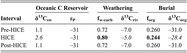
Table 4 Long description
Explanations of model assumptions are provided in the table caption along with citations of sources used to construct the model.
The table consists of three rows of six parameter values. The rows represent three time periods in the Late Ordovician: pre-H I C E, H I C E, and post-H I C E, and the specified parameters represent the starting conditions, the changed conditions during the H I C E, and the return to baseline in post-H I C E time. The six parameters are grouped into three sets of two parameters each. The first pair specifies the inferred change in the delta 13 C value of seawater during the H I C E and the photosynthetic fractionation factor, which is a constant in the model, the second set to the change in the modeled perturbation in the fraction of carbonate C weathering and its effect on the delta 13 C value of global river runoff during the H I C E, and the last pair to the change in the fraction of organic carbon buried as a consequence of the change in carbonate weathering contribution to the weathered C flux to the oceans, and the inferred steady-state change in delta 13 C org value of the organic carbon buried in the oceans.
Pre-H I C E interval (first row): the dissolved inorganic carbon of the oceanic reservoir (delta 13 C s w) is 1.1, and the photosynthetic fractionation factor (epsilon-P) is minus 31. The fraction of carbonate-derived carbon in riverine C-flux (fw-carb) is 0.72, and the terrestrial riverine C input (delta 13 C riv) is minus 7.0; the fraction of organic carbon buried (forg) is 0.260, and the isotopic composition of the organic carbon buried in oceanic sediments (delta 13 C org) is minus 31.0.
H I C E interval (Second row): the dissolved inorganic carbon of the oceanic reservoir (delta 13 C s w) is 2.6, and the photosynthetic fractionation factor (epsilon-P) is minus 31. The fraction of carbonate-derived carbon in riverine C-flux (fw-carb) is 0.80, and the terrestrial riverine C input (delta 13 C riv) is minus 5.0; the fraction of organic carbon buried (forg) is 0.244, and the isotopic composition of the organic carbon buried in oceanic sediments (delta 13 C org) is minus 28.4.
Post-H I C E interval (third row): the dissolved inorganic carbon of the oceanic reservoir (delta 13 C s w) is 1.1, and the photosynthetic fractionation factor (epsilon-P) is minus 31. The fraction of carbonate-derived carbon in riverine C-flux (fw-carb) is 0.72, and the terrestrial riverine C input (delta 13 C riv) is minus 7.0; the fraction of organic carbon buried (forg) is 0.260, and the isotopic composition of the organic carbon buried in oceanic sediments (delta 13 C org) is minus 31.0.
Considering factors that can change the δ13C value of the continental weathering flux rather than the burial efficiency of organic carbon during the glaciation has the advantage of being able to explain the origin of the positive CIE without contradicting the evidence for low TOC contents of sediments deposited during the Hirnantian sea-level lowstand. It is also consistent with sequence stratigraphic and geochemical evidence that positive CIEs through the Late Ordovician and early Silurian commonly correspond to sea-level lowstands (Ludvigson et al., Reference Ludvigson, Witzke and González2004; Saltzman & Young, Reference Saltzman and Young2005; Fanton & Holmden, Reference Fanton and Holmden2007; Immenhauser et al., Reference Immenhauser, Holmden and Patterson2008; Holmden et al., Reference Holmden, Mitchell and LaPorte2013; Husinec & Leslie, Reference Husinec and Leslie2022; Zimmt et al., Reference Zimmt, Holland, Desrochers, Jones and Finnegan2024). These considerations further suggest that increases in carbon burial and water column anoxia during the early mid Hirnantian may have been less extensive and persistent than previously supposed. Our argument here is that productivity during this interval shifted in character rather than increased – that productivity generally became both more localized and more variable in response to the climate variability that periodically altered local supplies of P, fixed N, and water column oxidation, and that these changes led to green-algal dominated phytoplankton communities that diplograptines were poorly equipped to utilize but that fit the needs of the exaptively well-equipped Neograptina.
The widespread anoxia associated with the rise of sea level concomitant with the retreat of the Hirnantian ice caps reflects the return to warm, stratified, oligotrophic oceanic conditions. Presumably those changes reshuffled the ecological deck yet again and resulted in the LOME-2 and LOME-3 turnover pulses (Finnegan et al., Reference Finnegan, Heim, Peters and Fischer2012b; Melchin et al., Reference Melchin, Mitchell, Holmden and Štorch2013; Harper et al., Reference Harper, Hammarlund and Rasmussen2014; Young et al., Reference Young, Benayoun and Kozik2020; Yang Sheng-chao et al., Reference Chao, Jun-peng and Wen-jie2021; Lu Yang-bo et al., Reference Yang-bo, Jun and Yu-xuan2022; Liang Yu et al., Reference Yu, Zerui Ray and Algeo2024; Zhang Jun-peng et al., Reference Jun-peng, Chao and Yang-yang2024). The linkage between anoxia, δ13CDIC, nutrient-related productivity changes, and species turnover during the LOME is supported by the correlation between the positive excursions in C and N isotopes that occur during glacial intervals in general and during the LOME interval in particular (reviewed in Algeo & Shen, Jun 2023). In the latter instance, δ15N values exhibit patterns of spatial variation among regions and among oceanic settings (relatively restricted shallow versus relatively open deep sites) that correspond with those of δ13C: large local changes in N cycling drove large local changes in C-cycling and isotopic fractionation that accentuated those of the global reservoir.
As we have argued earlier, the long-term record of graptolite turnover indicates that turnover among these zooplankton was intimately connected to fluctuations in the C-cycle (Cooper et al. Reference Cooper, Sadler, Munnecke and Crampton2014) in step with astronomically forced climate variability (Crampton et al. Reference Crampton, Meyers and Cooper2018). Interestingly, several sites that exhibit abrupt changes in δ13C and δ15N (e.g., Blackstone, Vinini Creek, see Figure 1) also exhibit abrupt changes in graptolite community composition, whereas at Wangjiawan, where the C and N stable isotope curves (Luo Gen-ming et al. Reference Gen-ming, Algeo and Ren-bin2016) exhibit extended rising limb and a brief peak in the lower M. persculptus Biozone interval also shows an extended turnover in the graptolite faunas (Fig. 1). Nanbazi and Dob’s Linn also exhibit a slow rising limb of the HICE through the M. extraordinarius Biozone strata with a distinct peak confined to the lower part of the M. persculptus Biozone there (Fig. 1) but unfortunately the Extraordinarius Chron interval at those sites produced few graptolite-bearing collections. Although it is possible that this pattern might be due in part to sedimentary condensation or hiatuses, we have found no independent sedimentological evidence for such at Blackstone or Vinini Creek, the latter of which also possesses a graptoliferous and apparently complete M. extraordinarius Biozone succession. Biomarker data, although also very sparse at this point, seem to follow a similar pattern – tracking rates of change in paleocommunity proxies and in N and C stable isotopes. Further studies are needed to test these relationships, but if these patterns are not artifacts, then it appears that local variation in the rate and timing of changes in N and C cycling may also have driven the pace of local population changes in plankton communities generally, including graptolites and the primary producers upon which they depended. We expect that these changes in N and C cycling likely affected many other organisms similarly.
4.7 Hirnantian Turnover Pulse Hypothesis
Building on her extensive work on Neogene mammalian faunas across Africa, Vrba (Reference Vrba1985, Reference Vrba1993, see also Barnosky Reference Barnosky2001, Faith & Behrensmeyer Reference Faith and Behrensmeyer2013), proposed the Turnover Pulse Hypothesis (TPH). She argued that alterations in habitat conditions brought about by Milankovitch cyclicity and climate change, especially during major episodes of cooling, led to pulses of migration, vicariance, and altered competition, which then led to turnover pulses – intervals of high origination and extinction – with durations on the scale of 100,000 yrs. Vrba (Reference Vrba1993) argued that the pairing of origination with extinction during a turnover pulse is especially informative, and that it indicated that these two outcomes are part of a single continuum of species’ responses to rapid habitat fragmentation and displacement: species undergo vicariance as metapopulations become disconnected, local populations shrink and either respond creatively to their shifting habitat through speciation or continue to decline into extinction. The TPH was originally developed as an explanation for the observed patterns of change in mammalian faunas across Africa during the late Neogene. A number of recent studies, however, suggest that similar dynamics affect marine plankton (e.g., Bendif et al., Reference Bendif, Nevado and Wong2019; Filatov et al., Reference Filatov, Bendif, Archontikis, Hagino and Rickaby2021; Beaufort et al., Reference Beaufort, Bolton and Sarr2022; Bendif et al., Reference Bendif, Probert and Archontikis2023).
The model of the Hirnantian mass extinction articulated by Brenchley et al. (Reference Brenchley, Marshall and Underwood2001, Reference Brenchley, Carden and Hints2003) reflects the general conception of mass extinction as a two-step process in which an intense interval of species losses occurs in response to some catastrophic forcing that persists through a depauperate interregnum of some duration that is followed ultimately by a return to “normal” conditions accompanied by evolutionary radiation and ecological recovery. We argued earlier that our results indicate that this model is poorly fit by the graptolite record during the end Ordovician events. The principal features of graptoloid species turnover during the LOME instead appear to correspond closely with those that Vrba identified as the likely drivers of a macroevolutionary turnover pulse. These include the coincidence of high rates of origination and extinction and their correspondence with times of strong habitat disruption caused by climate change and paced by Milankovitch cyclicity. Our data lack sufficient geographic resolution to demonstrate vicariance; however, the documented changes in metapopulation size do match predictions. The present analysis also generally lacks sufficient temporal resolution to demonstrate cyclicity in rates on the scale of 100 kyr throughout the Hirnantian, however, durations in the B3 bin set (equal sample size binning) during the interval of LOME-2 and LOME-3 are 100 kyr and the strong peaks in origination and extinction are fully captured (Fig. 6 A,B) and the p̂ and q̂ values for the B3 LOME-2 peak are the highest values obtained in any of our analyses. It is also noteworthy that the rapid changes in redox indicators at several sites in South China (e.g., Kozik et al., Reference Kozik, Young and Newby2022b; Jin Si-ding et al., Reference Si-ding, Hai-yang and Ming-cai2024; Wu Shuai-cai et al., Reference Shuai-cai, Lei and Min2024) and by δ13C and δ18O values at Anticosti Island, Laurentia (Mauviel et al., Reference Mauviel, Sinnesael and Desrochers2020; Zimmt et al., Reference Zimmt, Holland, Desrochers, Jones and Finnegan2024), among others, likely reflect astronomical forcing of climate variation. Such rapid fluctuations in redox and nutrient cycling undoubtedly added to the stress experienced by species during the LOME. Furthermore, that variability is likely to have empowered a selective ratchet that filtered organisms based on their capacity to accommodate the ensuing changes in habitats (size, location, and associated ecology). Dynesius and Jansson (Reference Dynesius and Jansson2000) referred to this phenomenon as “orbitally-forced range dynamics” or ORD. It is likely that the Neograptina, which were already adapted to the higher levels of climate variability present in temperate zone regions, reacted to the Hirnantian ORD inherently differently than the paleotropical Diplograptina and that this difference contributed to the observed clade-level selectivity of the graptolite species turnover: extinction in one and speciation in the other.
Further analysis of species’ biotope affiliation and geographic distribution through the LOME may permit testing of these ideas. Additional work is also needed to determine whether the observed replacement of diplograptines by neograptines was an expression of macroecological displacement driven by shared, limited resources or was simply a parallel but opposite response to ice-house conditions in the paleotropics.
4.8 Levels of Selection
Taken together, the principal features of graptolite species turnover during the LOME indicate that the late Katian oceanographic conditions produced by declining global temperature and the growth of the Gondwanan ice cap became increasingly inhospitable to the formerly dominant (wide-spread, abundant and long-lived) Diplograptina as their favored habitats shrank, were displaced off-shore and became more temporally unstable. These changes were probably accompanied by increased seasonal upwelling and regionally extensive, shallow anoxia (in contrast to the more enduring stratified systems and deeper, more stable oxygen-depleted deep-water layers of the preceding Boda warm interval) – changes that also altered patterns of carbon and nutrient cycling along with phytoplankton community compositions. This forced diplograptine species into smaller habitable areas and probably led to smaller and less well-connected metapopulations. It is reasonable to infer that the resulting ORD increased the difficulty of tracking their diminished realized niche and maintaining viable populations. In contrast, the invading neograptine species, having formerly occupied temperate to subpolar sites, were exaptively well suited to the new prevailing oceanographic conditions of the latest Katian and Hirnantian oceans. Neograptines appear to have taken advantage of the cool, well-oxygenated shelf settings and seasonal upwelling zones that were increasingly dominated by green algae. These features combined with Milankovitch-driven oscillations in oceanographic conditions and the resulting orbitally forced range dynamics of graptolite populations likely facilitated vicariance and speciation among the Neograptina in step with increased extinction among the Diplograptina. In short, Late Ordovician climate change actuated a ratchet-like selection regime that ultimately drove the entire diplograptine clade into extinction while simultaneously advancing the species diversity of the Neograptina. This level of selectivity appears to be a particularly severe version of what now seems to be a common feature of mass extinctions (Jablonski Reference Jablonski2005, Reference Jablonski2017b, a).
The observed clade-level selectivity of the LOME turnover indicates that the forces driving this turnover acted upon species as selective-individuals. Although the differential extinction and origination of diplograptine and neograptine species surely involved the differential birth and death of individual graptolite colonies, the defining feature of this turnover event is that none of the diplograptine species possessed a sufficient reservoir of suitable variance to adapt to and survive the Hirnantian icehouse. The survival of Paraorthograptus kimi into LOME-3 near the end of the Persculptus Chron past the demise of its clade-mates might be regarded as an exception to that generality; however, this ‘dead-clade walking’ (sensu Jablonski Reference Jablonski2002) merely proves the rule: species’ survival without descendants is a macroevolutionary death. Conversely, several neograptine species lineages evidently possessed apt properties (e.g., niche properties related to temperature, resource utilization, modes of reproduction, etc.) that enabled many of their species not only to survive but also to undergo speciation at rates that routinely exceeded extinctions through the Hirnantian icehouse interval and its aftermath and to undergo the structural innovations that seeded the unique graptolite lineages of the Silurian Period (Melchin et al. Reference Melchin, Mitchell, Naczk-Cameron, Junxuan and Loxton2011). Leaving aside the question of whether speciation and extinction are emergent, species-level traits or upward-caused effects of individual or population-level properties (see, for instance, Vrba & Gould Reference Vrba and Gould1986, Myers & Saupe Reference Myers and Saupe2013, Jablonski Reference Jablonski2017b), it is clear that the lack of variance for these key macroevolutionary traits among the diplograptines and its residence exclusively among neograptines means that there cannot have been selection for differential survivorship and proliferation within these species (see Lloyd & Gould Reference Lloyd and Gould1993, Gould & Lloyd Reference Gould and Lloyd1999). Instead, selection can only have acted relative to variance in these traits among species, presumably as a consequence of their clade-specific apomorphies – that is, strictly via species selection. Indeed, selectivity of extinction and origination probabilities among clades (especially during intervals of intense selection as in the LOME) may be one of the most fruitful sources of direct evidence of species selection available in the fossil record.
5 Conclusions
Graptolite turnover from the latest Katian into the earliest Silurian exhibited an extraordinary level of clade selectivity. The Neograptina experienced high rates of speciation simultaneously with the high rates of extinction among diplograptine species; extinctions that ultimately led to the complete extirpation of the Diplograptina. The proliferation of the Neograptina appears to have resulted in some significant measure as an exaptive response to Hirnantian icehouse conditions, which created favorable circumstances in the paleotropics for the immigration of several temperate neograptine species. Their subsequent macroevolutionary radiation led to the origination of a series of novel graptolite clades including the uni-biserial Dimorphograpidae, the reticulated Retiolitinae and the wildly diverse Monograptidae (Melchin et al. Reference Melchin, Mitchell, Naczk-Cameron, Junxuan and Loxton2011, Sadler et al. Reference Sadler, Cooper and Melchin2011, Bapst et al. Reference Bapst, Bullock, Melchin, Sheets and Mitchell2012). Thus, although the LOME is often regarded as having exerted little selective effect on either the clade composition or ecological structure of marine communities (e.g., McGhee Jr et al. Reference McGhee, Sheehan, Bottjer and Droser2012, Krug & Patzkowsky Reference Krug and Patzkowsky2015, Bush et al. Reference Bush, Wang, Payne and Heim2020), planktic graptolites experienced the episode quite differently. This, in turn, suggests that the graptolite response to the LOME may provide a particularly sensitive indicator of the causes of that event.
Diplograptine and neograptine species occur together in the great preponderance of latest Katian and early Hirnantian samples and so they must have occupied more or less the same sites and water masses most of that time. This fact considered together with the trajectory of graptolite species extinction and origination during the LOME events and the strong clade-level selectivity of that turnover, indicate that oceanic anoxia was not a primary driver of species extinction among the zooplankton during the LOME. Instead, the widespread anoxia appears to have been a symptom of the altered oceanographic and climatic conditions associated with the Hirnantian glaciation, and in particular, reflected changes in oceanic circulation, nutrient supply, and phytoplankton productivity. We suggest that it was primarily these features, in combination with changes in habitat area and the displacement of habitats offshore, that drove graptolite species turnover during the LOME. Similarly, correlations between species turnover more generally and local facies and geochemical proxies may reflect common causes in which each was responding to the underlying paleoclimatic and oceanographic disruptions created during greenhouse–icehouse transitions. The long-term, multiphased history of turnover among graptolites through the Late Ordovician, with its coordinated rise and fall of origination and extinction rates in synchrony with climate-driven habitat change suggests that the LOME was not a unitary or even two-phased mass extinction at all but an extended episode of multiple successive turnover pulses (a la Vrba Reference Vrba1985, Reference Vrba1993) paced by orbital periodicity during the relatively short-lived but intense late Katian–Hirnantian glaciation and the following greenhouse.
6 Afterthought: The Late Ordovician Timescale
Zhang et al. (Reference Zhang, Yang and Sahy2025) present several new U-Pb radiometric dates derived from zircons sampled from ash beds in three sections in South China, including the Wangjiawan Hirnantian GSSP section. Based on these age results, Zhang et al. conclude that the Hirnantian Age lasted for only ~320 Kyr and that the P. pacificus Biozone interval had a duration of ~1 myr – much shorter than the intervals in our scaled composite (1.2 myr and 1.8 myr, respectively). These new dates indicate that the three glacial advance–retreat cycles (Mirus Subchron to early Persculptus Chron) that largely coincide with the LOME had durations of approximately 120 Kyr each, similar to those in the Quaternary glacial epoch. The Zhang et al. (Reference Zhang, Yang and Sahy2025) timescale also suggests that the duration of our B1–B3 bins in the Pacificus Chron interval are also about 120 kyr and those in the Mirus to Ascensus interval may have durations of only ~52 Kyr. These durations, in turn, suggest that the three major turnover pulses documented here correspond even more closely with those that Vrba (Reference Vrba1985, Reference Vrba1993) identified in her model. The new dates also suggest, of course, that the LOME may have been much more intense than our present turnover rates reveal, with peak extinction and origination rates some four times higher than our rates and an increased contrast in rates between those in pre-Mirus Chron times and those in the main LOME turnover pulses. These revisions, however, do not alter the relative duration of three main turnover phases documented herein, which are not consistent with the claim in Zhang et al. (Reference Zhang, Yang and Sahy2025) that the LOME consisted of an extended, low-intensity phase in the early Hirnantian and a shorter, higher-rate turnover confined to the immediate postglacial interval. That apparent difference in rates through the course of the LOME again appears to be largely an artifact of the sampled record (as discussed earlier) and the general problem inherent in the comparison of rates measured over different interval lengths (see, for instance, Sadler Reference Sadler1981, Sheets & Mitchell Reference Sheets and Mitchell2001, Harmon et al. Reference Harmon, Pennell and Henao-Diaz2021).
Acknowledgements
MJM acknowledges ongoing financial support from a Natural Sciences and Engineering Council Discovery Grant. We thank David W. Bapst and an anonymous reviewer for their carefully considered suggestions on an earlier draft, which substantially helped us improve the manuscript.
Editor-in-Chief
Brenda R. Hunda
Cincinnati Museum Center
About the Series
The Elements of Paleontology series is a publishing collaboration between the Paleontological Society and Cambridge University Press. The series covers the full spectrum of topics in paleontology and paleobiology, and related topics in the Earth and life sciences of interest to students and researchers of paleontology.
The Paleontological Society is an international nonprofit organization devoted exclusively to the science of paleontology: invertebrate and vertebrate paleontology, micropaleontology, and paleobotany. The Society’s mission is to advance the study of the fossil record through scientific research, education, and advocacy. Its vision is to be a leading global advocate for understanding life’s history and evolution. The Society has several membership categories, including regular, amateur/avocational, student, and retired. Members, representing some 40 countries, include professional paleontologists, academicians, science editors, Earth science teachers, museum specialists, undergraduate and graduate students, postdoctoral scholars, and amateur/avocational paleontologists.

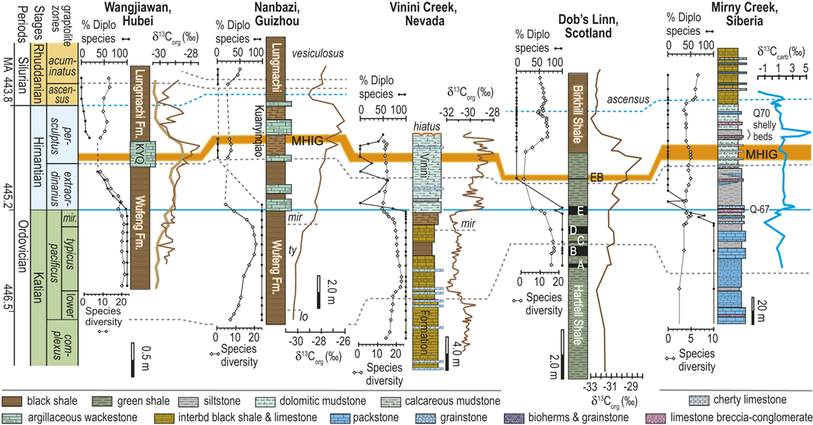
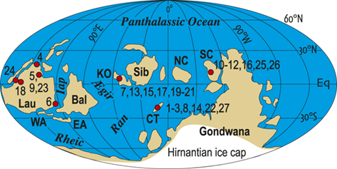
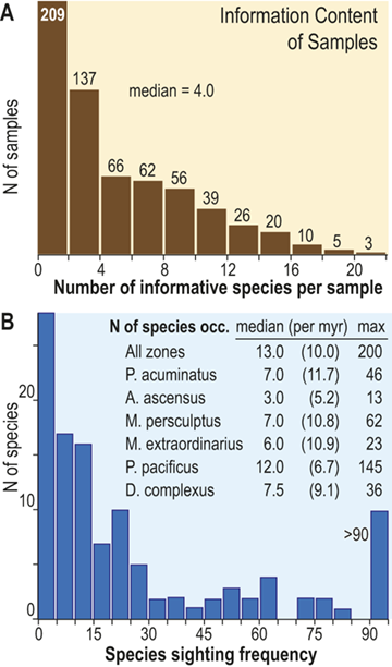
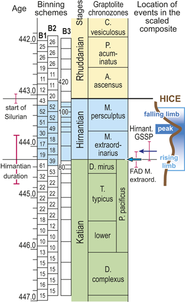
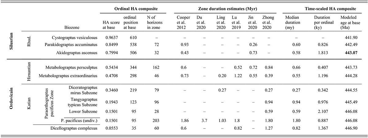
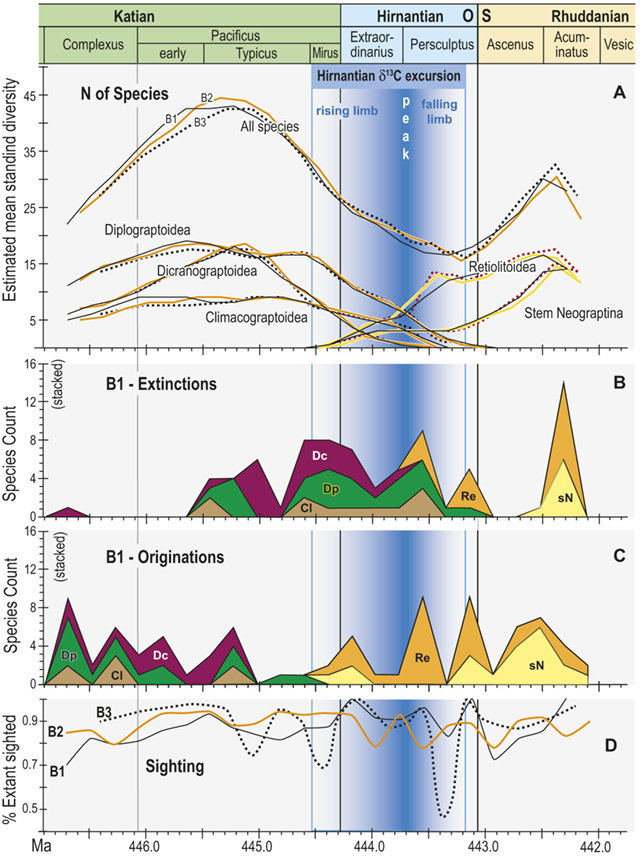
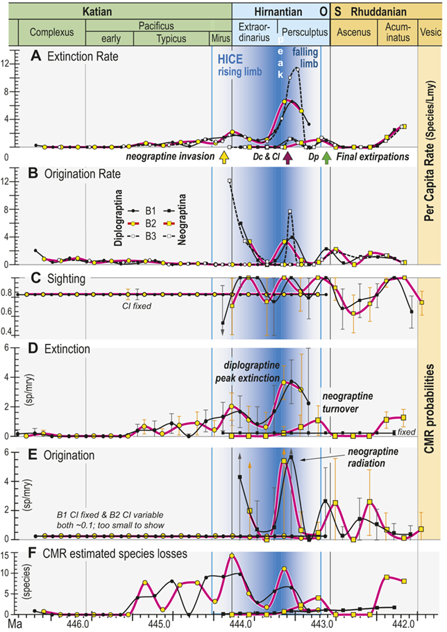
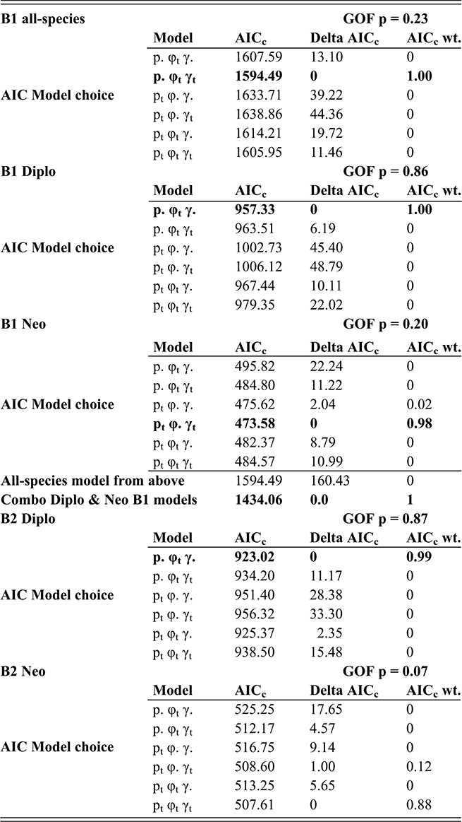
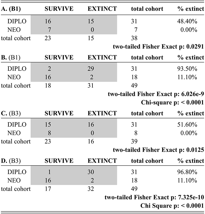
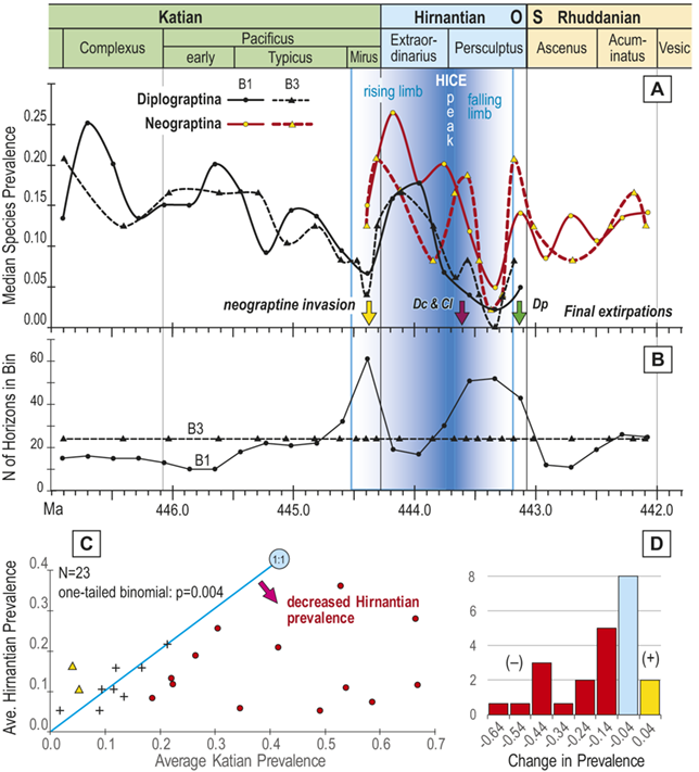
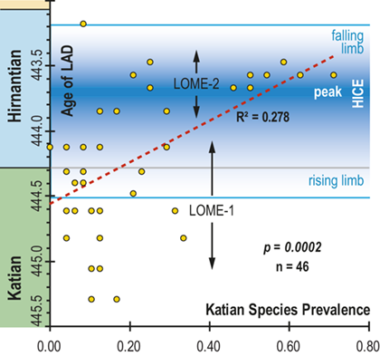
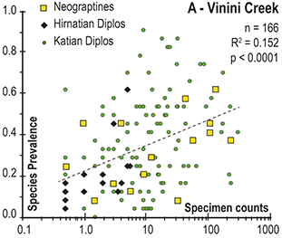
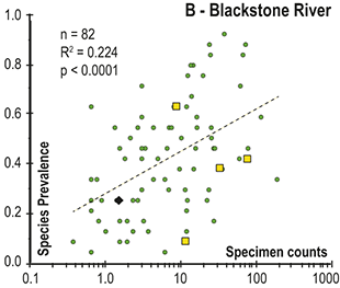
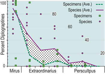
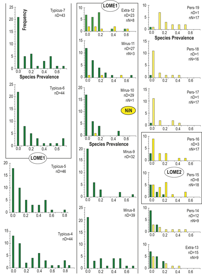
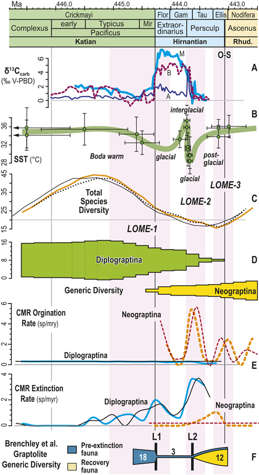
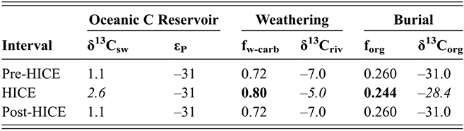

 Open access