


NOMENCLATURE
 ${c_{cr1}},{c_{cr2}}$
constant coefficients in conventional QCR
- ${c_{cr3}},{c_{cr4}}$
additional constant coefficients in extended QCR
- ${\tilde c_{cr3}}$
effective additional constant coefficient
$\left( { = {c_{cr3}} - {c_{cr4}}} \right)$- DNS
direct numerical simulation
- h
half-height of channel/duct
- k
turbulent kinetic energy
- LES
large-eddy simulation
- LEVM
linear eddy-viscosity model
- p
pressure
- P
production of turbulent kinetic energy
- QCR
quadratic constitutive relation
- r
radius of pipe
- RANS
Reynolds-averaged Navier–Stokes
- Re $_\tau $
friction Reynolds number
- Re $_\theta $
Reynolds number based on boundary-layer momentum thickness
- ${S_{ij}}$
stress tensor
- $S_{ij}^*$
traceless stress tensor
- ${x_i} = \left\{ {x,y,z} \right\}$
streamwise, wall-normal and spanwise spatial coordinate
- ${u_b}$
bulk streamwise velocity
- ${u_i} = \left\{ {u,v,w} \right\}$
mean velocity in the
$\left\{ {x,y,z} \right\}$ direction- ${u_{i}}^{'} = \left\{ u^{'},v^{'},w^{'} \right\}$
turbulent velocity fluctuation in the
$\left\{ {x,y,z} \right\}$ direction- ${u_\tau }$
friction velocity
- ${y^ + }$
wall-normal coordinate in wall units


Greek symbol
- $\delta $
boundary-layer thickness
- ${\delta _{ij}}$
Kronecker delta
- ${\delta _{{\rm{ref}}}}$
flow thickness: channel half-height, boundary-layer thickness, pipe radius
- $\varepsilon $
dissipation of turbulent kinetic energy
- ${\mu _t}$
eddy viscosity
- $\rho $
density
- ${\tilde \sigma _{ij}}$
rescaled estimate of the turbulent stress tensor
$\left( { = {{\tilde \tau }_{ij}}/{\mu _t}} \right)$- ${\tau _{ij}}$
turbulent stress tensor
- ${\tilde \tau _{ij}}$
turbulent stress tensor estimated using an eddy-viscosity model
- ${\omega _i} = \left\{ {{\omega _x},{\omega _y},{\omega _z}} \right\}$
mean vorticity component in the
$\left\{ {x,y,z} \right\}$ direction- ${\Omega _{ij}}$
vorticity tensor, with respect to an inertial reference frame


1.0 INTRODUCTION
Despite the availability of high-fidelity computational approaches, such as large-eddy simulations (LES) and direct numerical simulations (DNS), the prohibitive cost of these approaches means that, for design purposes, Reynolds-averaged Navier–Stokes (RANS) methods remain ubiquitous in the aerospace industry. Practical applications in this industry often feature complex geometries, such as wing–body junctions and turbine blade–hub junctions, where anisotropies in the turbulent stress distributions are known to influence the mean flow(Reference Gessner and Jones1). In such applications, accurate calculations of the turbulent stresses are therefore paramount in order to reliably predict the overall flow field.
RANS computations do not obtain the turbulent stresses directly but instead use a prescribed turbulence model to estimate the eddy viscosity,  ${\mu _t}$, from the mean flow data. An ‘eddy-viscosity model’ is then used to evaluate an approximation the turbulent stresses from
  ${\mu _t}$. Linear eddy-viscosity models (LEVMs) have remained popular due to their simplicity and low computational cost, as compared to more involved closure models, despite providing somewhat inaccurate turbulent stress estimates. For example, LEVMs result in a simple distribution of normal turbulent stresses,
  $\overline {u^{\prime}u^{\prime}} = \overline {v^{\prime}v^{\prime}} = \overline {w^{\prime}w^{\prime}} $. This can be particularly problematic in the complex geometries often encountered in practical applications, where normal stress anisotropy is expected to influence the mean flow. As a result, LEVMs are unable to reliably predict the flow in jets, streamwise corners or separated boundary layers(Reference Wilcox2).
One approach to extend the capabilities of LEVMs with only a mild increase in complexity is to consider terms that are quadratic in the mean stress and vorticity tensors, when evaluating the turbulent stress tensor. Spalart developed this type of quadratic eddy-viscosity model, termed the quadratic constitutive relation (QCR), which still relates the eddy viscosity with the turbulent stresses using only properties of the mean flow rather than any variables specific to the turbulence model in use(Reference Spalart3,Reference Mani, Babcock, Winkler and Spalart4) .
The key success of QCR has been the prediction of the flow in geometries featuring streamwise corners. Here, experiments and direct numerical simulations show the presence of a counter-rotating vortex pair. Whilst RANS computations using linear eddy-viscosity models do not capture these vortices, QCR is able to successfully predict the presence of a vortex pair in the corner flow(Reference Mani, Babcock, Winkler and Spalart4,Reference Bisek5) . The improvement in flow prediction has been shown to result in a better estimate of corner separation(Reference Rumsey, Carlson and Ahmad6), including shock-induced separation in transonic and supersonic flows(Reference Dandois7). However, even these predictions are limited in their accuracy(Reference Rumsey, Carlson and Ahmad6,Reference Dandois7) . Furthermore, when the constant  ${c_{cr1}}$ (which, in practice, is treated like a tuning parameter) exceeds the recommended value of 0.3, Leger et al. have noted the appearance of additional non-physical vortices(Reference Leger, Bisek and Poggie8).
More generally, with the exception of the successful prediction of large streamwise vortices in Couette flow(Reference Spalart, Garbaruk and Strelets9), the improvement in the computation of other complex flow fields has been somewhat modest. Of course, a perfect prediction of turbulent stresses for all types of flow is not attainable using an approach with a small number of calibration constants. However, the limited success in mean flow prediction suggests that the inclusion of QCR terms does not significantly improve estimates of turbulent stresses. In order to investigate the capabilities and limitations of QCR, this paper considers an extension with additional quadratic terms not included in the original definitions.
The aim of the analysis is to investigate the capabilities of three eddy-viscosity models: an LEVM, conventional QCR and the proposed extension to QCR. RANS computations of a flow problem require a prescribed turbulence model and so the corresponding results would be dependent on the chosen turbulence model. Instead, the procedure adopted in this paper directly tests the eddy-viscosity models themselves. To do so, the impact of different eddy-viscosity models on turbulent stress anisotropy is assessed by using accurate values of mean velocity and turbulent stresses from direct numerical simulations (DNS).
For several flow fields, published DNS velocity statistics are used to determine the distribution of  ${\mu _t}$ that would best relate the relevant turbulent stresses to the mean flow. This can be considered as the best-case scenario for an hypothetical RANS simulation using a ‘perfect’ turbulence model for that particular flow, even if such a model does not exist in reality. From the DNS-obtained eddy viscosity, the turbulent stresses are predicted for each eddy-viscosity model under investigation and are then compared with the ‘correct’ stresses reported by DNS. This comparison provides an evaluation of how well the turbulent stresses, which can have a significant impact on the mean flow, are predicted by the various eddy-viscosity models.
The particular DNS data sets used in this study are all incompressible flows at moderate Reynolds numbers, as detailed in Table 1. These flow fields include canonical cases — channel flow(Reference Bernardini, Pirozzoli and Orlandi10,Reference Hoyas and Jiménez11) , boundary layers(Reference Sillero, Jiménez and Moser12–Reference Schlatter, Li, Brethouwer, Johansson and Henningson14) and pipe flow(Reference El Khoury, Schlatter, Noorani, Fischer, Brethouwer and Johansson15) — as well as more complex flows, such as the separated boundary layers(Reference Coleman, Rumsey and Spalart16) and square duct flow(Reference Pirozzoli, Modesti, Orlandi and Grasso17). The profiles from these different flow families exhibit quite distinct turbulent stress distributions, especially away from the wall(Reference Monty, Hutchins, Ng, Marusic and Chong18), allowing a wide range of flow cases to be studied.
Direct numerical simulations of incompressible flows analysed in this paper. Reτ is the friction Reynolds number, and Re $_\theta $ is the Reynolds number based on boundary-layer momentum thickness

 $^{{\rm{(}}a)}$This study was performed using well-resolved large-eddy simulations.
Note that since RANS simulations may not exactly compute the correct mean flow, the adopted procedure does not quite equate to an assessment of how well an actual RANS calculation would predict the turbulent stresses. However, the validity of this process improves with increased accuracy of RANS simulations and the fundamental aim of RANS is to produce the correct mean flow, so this approach can still be considered instructive. Furthermore, the DNS-based analysis has the significant advantage that it is independent of any turbulence model and so provides a direct test of the eddy-viscosity models themselves.
2.0 The quadratic constitutive relation (QCR)
Linear eddy-viscosity models estimate the time-averaged turbulent stress tensor,  ${\tau _{ij}} = - \rho \overline {{u_{i}^{\prime}} {u_{j}^{\prime}}} $, using the Boussinesq assumption:
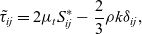 \begin{equation}{\tilde \tau _{ij}} = 2{\mu _t}S_{ij}^* - \frac{2}{3}\rho k{\delta _{ij}},\end{equation}
where  ${\tilde \tau _{ij}}$ is the estimated turbulent stress tensor and
  ${\mu _t}$ is the eddy viscosity. In this equation, the traceless stress tensor
 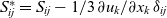 $S_{ij}^* = {S_{ij}} - 1/3{\kern 1pt} \partial {u_k}/\partial {x_k}{\kern 1pt} {\delta _{ij}}$, with
  ${\delta _{ij}}$ denoting the Kronecker delta, and
  ${S_{ij}} = 1/2\left( {\partial {u_i}/\partial {x_j} + \partial {u_j}/\partial {x_i}} \right)$. The mean velocity components
  ${u_i} = \left\{ {u,v,w} \right\}$ correspond to the spatial coordinates
  ${x_i} = \left\{ {x,y,z} \right\}$ in the streamwise, wall-normal and spanwise directions, respectively. The density is given by
  $\rho $, and k corresponds to the turbulent kinetic energy. Note that the second term,
  $2/3\rho k{\delta _{ij}}$, is neglected in one-equation turbulence models, which have instead:
 \begin{equation}{\tilde \tau _{ij}} = 2{\mu _t}S_{ij}^*{\rm{.}}\end{equation}
There are three iterations of the quadratic constitutive relation, developed by Spalart. The original statement of the relation, QCR-2000(Reference Spalart3), is defined by:
 \begin{equation}{\tilde \tau _{ij}} = 2{\mu _t}S_{ij}^* - \frac{4{c_{cr1}}{\mu _t}}{\sqrt {{S_{kl}}{S_{kl}} + {\Omega _{kl}}{\Omega _{kl}}} }\left[ {{\Omega _{ik}}S_{kj}^* - S_{ik}^*{\Omega _{kj}}} \right],\end{equation}
where the vorticity tensor  ${\Omega _{ij}} = 1/2\left( {\partial {u_i}/\partial {x_j} - \partial {u_j}/\partial {x_i}} \right)$ or, in applications with rotation or curvature, would be defined with respect to an inertial reference frame(Reference Shur, Strelets, Travin and Spalart19). Note that since this modification uses only mean-flow properties, it can be applied to any single-equation or multi-equation turbulence model that is based on a linear eddy-viscosity model. For turbulence models that provide the turbulent kinetic energy, k, the additional term
  $2/3\rho k{\delta _{ij}}$ can be included in the eddy-viscosity relation:
 \begin{equation}{\tilde \tau _{ij}} = 2{\mu _t}S_{ij}^* - \frac{4{c_{cr1}}{\mu _t}}{\sqrt {{S_{kl}}{S_{kl}} + {\Omega _{kl}}{\Omega _{kl}}} }\left[ {{\Omega _{ik}}S_{kj}^* - S_{ik}^*{\Omega _{kj}}} \right] - \frac{2}{3}\rho k{\delta _{ij}}.\end{equation}
An extension to this framework, QCR-2013(Reference Mani, Babcock, Winkler and Spalart4), was proposed for turbulence models that do not provide k. This formulation includes an additional term:
 \begin{equation}{\tilde \tau _{ij}} = 2{\mu _t}S_{ij}^* - {{4{c_{cr1}}{\mu _t}} \over {\sqrt {{S_{kl}}{S_{kl}} + {\Omega _{kl}}{\Omega _{kl}}} }}\left[ {{\Omega _{ik}}S_{kj}^* - S_{ik}^*{\Omega _{kj}}} \right] - {c_{cr2}}{\mu _t}\left[ {\sqrt {2S_{kl}^*S_{kl}^*} } \right]{\delta _{ij}}.\end{equation}
The constants  ${c_{cr1}}$ and
  ${c_{cr2}}$ were proposed as
  $0.3$ and
  $2.5$, respectively, after calibration in the outer part of an equilibrium turbulent boundary layer(Reference Mani, Babcock, Winkler and Spalart4). The additional term,
  ${c_{cr2}}{\mu _t}\left[ {\sqrt {2S_{kl}^*S_{kl}^*} } \right]{\delta _{ij}}$, approximately accounts for the
  $2/3\rho k{\delta _{ij}}$ term in the Boussinesq equation (Equation (1)), which had been omitted in Equations (2) and (3).
Note that this term contributes  $\partial /\partial {x_j}\left( {{c_{cr2}}{\mu _t}\left[ {\sqrt {2S_{kl}^*S_{kl}^*} } \right]{\delta _{ij}}} \right) = \partial /\partial {x_i}\left( {{c_{cr2}}{\mu _t}\left[ {\sqrt {2S_{kl}^*S_{kl}^*} } \right]} \right)$ to the momentum equation. This is simply a gradient in the
  ${x_i}$ direction and so takes the same form as the pressure gradient term,
  $\partial p/\partial {x_i}$. Therefore, even if this term was not explicitly included, its effect would be implicitly incorporated in the pressure distribution, and so the term does not affect the mean velocity distribution. As a result, the inclusion of this particular term is not intended to directly improve prediction of the mean velocity field but instead allows the distribution of pressure and normal turbulent stresses to better match the true values.
Similarly, the additional term in Equation (5) also provides a means to extend the linear eddy-viscosity model for one-equation models (Equation (2)) by introducing an estimated, non-zero turbulent kinetic energy:
 \begin{equation}{\tilde \tau _{ij}} = 2{\mu _t}S_{ij}^* - {c_{cr2}}{\mu _t}\left[ {\sqrt {2S_{kl}^*S_{kl}^*} } \right]{\delta _{ij}}{\rm{.}}\end{equation}
A recent version of the model, termed QCR-2020, has been proposed by Rumsey et al. (Reference Rumsey, Carlson, Pulliam and Spalart20). In this formulation, the constants,  ${c_{cr1}}$ and
  ${c_{cr2}}$, are no longer assumed to be spatially uniform but are replaced with equivalent coefficients containing wall-normal dependency, which vary from one value at the walls to a different one near the boundary-layer edge. Given the relative infancy of the QCR-2020 extension and its inherent added complexity, this paper instead focuses on QCR-2013, which has constant coefficient values and whose effect has been studied extensively(Reference Bisek5–Reference Leger, Bisek and Poggie8).
3.0 An extension to the quadratic constitutive relation
The modest success of QCR in most flow fields suggests that the turbulent stress predictions need to be further improved. One possible approach is to revisit the expansion developed by Gatski and Speziale(Reference Gatski and Speziale21), whose first two terms correspond to the linear term (Equation (2)) and to the QCR-2000 quadratic term (Equation (3)). To improve the estimate of turbulent stresses, it may therefore be beneficial to include additional terms in the eddy-viscosity model from the expansion.
In fact, it is not necessary to immediately extend the eddy-viscosity model to cubic terms because there are two additional terms, not included in QCR-2013, which are quadratic in S and  $\Omega $ and which satisfy the fundamental contraction (
 $\overline {{u_i}^{\prime} {u_i}^{\prime}} = k$) and symmetry (
 $\overline {u_i^{\prime}u_j^{\prime}} = \overline {u_j^{\prime}u_i^{\prime}} $) properties(Reference Pope22,Reference Pope23) . If it is assumed that the scaling with
  ${\mu _t}$, S and
  $\Omega $ of all these terms is the same as for the quadratic term in QCR-2013, we obtain:
 \begin{align} {{\tilde \tau }_{ij}} = 2{\mu _t}S_{ij}^* & \underbrace { - {{4{c_{cr1}}{\mu _t}} \over {\sqrt {{S_{kl}}{S_{kl}} + {\Omega _{kl}}{\Omega _{kl}}} }}\left[ {{\Omega _{ik}}S_{kj}^* - S_{ik}^*{\Omega _{kj}}} \right]}_{\rm{A}} - {c_{cr2}}{\mu _t}\left[ {\sqrt {2S_{kl}^*S_{kl}^*} } \right]{\delta _{ij}}\nonumber \\
&{\underbrace { - {{4{c_{cr3}}{\mu _t}} \over {\sqrt {{S_{kl}}{S_{kl}} + {\Omega _{kl}}{\Omega _{kl}}} }}\left[ {S_{ik}^*S_{kj}^* - \frac{1}{3}S_{kl}^*S_{kl}^*{\delta _{ij}}} \right]}_{\rm{B}}} \\
& {\underbrace { + {{4{c_{cr4}}{\mu _t}} \over {\sqrt {{S_{kl}}{S_{kl}} + {\Omega _{kl}}{\Omega _{kl}}} }}\left[ {{\Omega _{ik}}{\Omega _{kj}} + \frac{1}{3}{\Omega _{kl}}{\Omega _{kl}}{\delta _{ij}}} \right]}_{\rm{C}}.}\nonumber \end{align}
\begin{align} {{\tilde \tau }_{ij}} = 2{\mu _t}S_{ij}^* & \underbrace { - {{4{c_{cr1}}{\mu _t}} \over {\sqrt {{S_{kl}}{S_{kl}} + {\Omega _{kl}}{\Omega _{kl}}} }}\left[ {{\Omega _{ik}}S_{kj}^* - S_{ik}^*{\Omega _{kj}}} \right]}_{\rm{A}} - {c_{cr2}}{\mu _t}\left[ {\sqrt {2S_{kl}^*S_{kl}^*} } \right]{\delta _{ij}}\nonumber \\
&{\underbrace { - {{4{c_{cr3}}{\mu _t}} \over {\sqrt {{S_{kl}}{S_{kl}} + {\Omega _{kl}}{\Omega _{kl}}} }}\left[ {S_{ik}^*S_{kj}^* - \frac{1}{3}S_{kl}^*S_{kl}^*{\delta _{ij}}} \right]}_{\rm{B}}} \\
& {\underbrace { + {{4{c_{cr4}}{\mu _t}} \over {\sqrt {{S_{kl}}{S_{kl}} + {\Omega _{kl}}{\Omega _{kl}}} }}\left[ {{\Omega _{ik}}{\Omega _{kj}} + \frac{1}{3}{\Omega _{kl}}{\Omega _{kl}}{\delta _{ij}}} \right]}_{\rm{C}}.}\nonumber \end{align}
For a parallel mean shear flow,  $u\left( y \right)$, where
  $v = w = 0$, the two new terms (B and C) are different to the original QCR-2000 quadratic term (A) but are identical to each other:
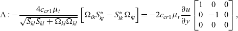 \begin{equation}{\rm{A}}: - \frac{{4{c_{cr1}}{\mu _t}}}{{\sqrt {{S_{kl}}{S_{kl}} + {\Omega _{kl}}{\Omega _{kl}}} }}\left[ {{\Omega _{ik}}S_{kj}^* - S_{ik}^*{\Omega _{kj}}} \right] = - 2{c_{cr1}}{\mu _t}\frac{{\partial u}}{{\partial y}}\left[ {\begin{array}{*{20}{c}}
100 \\
0{ - 1}0 \\
000 \\
\end{array}} \right],\end{equation}
\begin{equation}{\rm{A}}: - \frac{{4{c_{cr1}}{\mu _t}}}{{\sqrt {{S_{kl}}{S_{kl}} + {\Omega _{kl}}{\Omega _{kl}}} }}\left[ {{\Omega _{ik}}S_{kj}^* - S_{ik}^*{\Omega _{kj}}} \right] = - 2{c_{cr1}}{\mu _t}\frac{{\partial u}}{{\partial y}}\left[ {\begin{array}{*{20}{c}}
100 \\
0{ - 1}0 \\
000 \\
\end{array}} \right],\end{equation}
 \begin{equation}{\rm{B}}: - \frac{{4{c_{cr3}}{\mu _t}}}{{\sqrt {{S_{kl}}{S_{kl}} + {\Omega _{kl}}{\Omega _{kl}}} }}\left[ {S_{ik}^*S_{kj}^* - \frac{1}{3}S_{kl}^*S_{kl}^*{\delta _{ij}}} \right] = - \frac{1}{3}{c_{cr3}}{\mu _t}\frac{{\partial u}}{{\partial y}}\left[ {\begin{array}{*{20}{c}}
100 \\
010 \\
00{ - 2} \\
\end{array}} \right],\end{equation}
\begin{equation}{\rm{B}}: - \frac{{4{c_{cr3}}{\mu _t}}}{{\sqrt {{S_{kl}}{S_{kl}} + {\Omega _{kl}}{\Omega _{kl}}} }}\left[ {S_{ik}^*S_{kj}^* - \frac{1}{3}S_{kl}^*S_{kl}^*{\delta _{ij}}} \right] = - \frac{1}{3}{c_{cr3}}{\mu _t}\frac{{\partial u}}{{\partial y}}\left[ {\begin{array}{*{20}{c}}
100 \\
010 \\
00{ - 2} \\
\end{array}} \right],\end{equation}
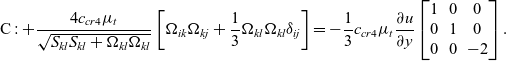 \begin{equation}{\rm{C}}:{\rm{ + }}\frac{{{\rm{4}}{{\rm{c}}_{{\rm{cr4}}}}{\mu _{\rm{t}}}}}{{\sqrt {{{\rm{S}}_{{\rm{kl}}}}{{\rm{S}}_{{\rm{kl}}}}{\rm{ + }}{\Omega _{{\rm{kl}}}}{\Omega _{{\rm{kl}}}}} }}\left[ {{\Omega _{{\rm{ik}}}}{\Omega _{{\rm{kj}}}}{\rm{ + }}\frac{{\rm{1}}}{{\rm{3}}}{\Omega _{{\rm{kl}}}}{\Omega _{{\rm{kl}}}}{\delta _{{\rm{ij}}}}} \right]{\rm{ = - }}\frac{{\rm{1}}}{{\rm{3}}}{{\rm{c}}_{{\rm{cr4}}}}{\mu _{\rm{t}}}\frac{{\partial {\rm{u}}}}{{\partial {\rm{y}}}}\left[ {\begin{array}{*{20}{c}}
100 \\
010 \\
00{ - 2} \\
\end{array}} \right].\end{equation}
\begin{equation}{\rm{C}}:{\rm{ + }}\frac{{{\rm{4}}{{\rm{c}}_{{\rm{cr4}}}}{\mu _{\rm{t}}}}}{{\sqrt {{{\rm{S}}_{{\rm{kl}}}}{{\rm{S}}_{{\rm{kl}}}}{\rm{ + }}{\Omega _{{\rm{kl}}}}{\Omega _{{\rm{kl}}}}} }}\left[ {{\Omega _{{\rm{ik}}}}{\Omega _{{\rm{kj}}}}{\rm{ + }}\frac{{\rm{1}}}{{\rm{3}}}{\Omega _{{\rm{kl}}}}{\Omega _{{\rm{kl}}}}{\delta _{{\rm{ij}}}}} \right]{\rm{ = - }}\frac{{\rm{1}}}{{\rm{3}}}{{\rm{c}}_{{\rm{cr4}}}}{\mu _{\rm{t}}}\frac{{\partial {\rm{u}}}}{{\partial {\rm{y}}}}\left[ {\begin{array}{*{20}{c}}
100 \\
010 \\
00{ - 2} \\
\end{array}} \right].\end{equation}
The conventional QCR term (A) was chosen because it increases  $\overline {{u^{\prime}}{u^{\prime}}} $ and decreases
  $\overline {{v^{\prime}}{v^{\prime}}} $ such that
 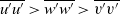 $\overline {{u^{\prime}}{u^{\prime}}} \gt \overline {{w^{\prime}}{w^{\prime}}} \gt \overline {{v^{\prime}}{v^{\prime}}} $, which is known to hold for parallel mean shear flows
  $u\left( y \right)$, such as boundary layers(Reference Pope22). However, the other quadratic terms (B and C) are of the same order in the expansion about S and
  $\Omega $, so these terms might be expected to have an influence of similar magnitude as term A.
In general, as well as evaluating to identical expressions for a parallel mean shear flow, terms B and C also tend to the same expression as each other for any fully developed flow where  $u \gg v,w$. Whilst a long-term aim is to discriminate between these two terms, for now the problem is therefore simplified by considering instead:
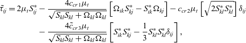 \begin{align} {{\tilde \tau }_{ij}} = 2{\mu _t}S_{ij}^* & - {{4{c_{cr1}}{\mu _t}} \over {\sqrt {{S_{kl}}{S_{kl}} + {\Omega _{kl}}{\Omega _{kl}}} }}\left[ {{\Omega _{ik}}S_{kj}^* - S_{ik}^*{\Omega _{kj}}} \right] - {c_{cr2}}{\mu _t}\left[ {\sqrt {2S_{kl}^*S_{kl}^*} } \right]{\delta _{ij}} \nonumber\\
& - {{4{{\tilde c}_{cr3}}{\mu _t}} \over {\sqrt {{S_{kl}}{S_{kl}} + {\Omega _{kl}}{\Omega _{kl}}} }}\left[ {S_{ik}^*S_{kj}^* - {1 \over 3}S_{kl}^*S_{kl}^*{\delta _{ij}}} \right], \end{align}
\begin{align} {{\tilde \tau }_{ij}} = 2{\mu _t}S_{ij}^* & - {{4{c_{cr1}}{\mu _t}} \over {\sqrt {{S_{kl}}{S_{kl}} + {\Omega _{kl}}{\Omega _{kl}}} }}\left[ {{\Omega _{ik}}S_{kj}^* - S_{ik}^*{\Omega _{kj}}} \right] - {c_{cr2}}{\mu _t}\left[ {\sqrt {2S_{kl}^*S_{kl}^*} } \right]{\delta _{ij}} \nonumber\\
& - {{4{{\tilde c}_{cr3}}{\mu _t}} \over {\sqrt {{S_{kl}}{S_{kl}} + {\Omega _{kl}}{\Omega _{kl}}} }}\left[ {S_{ik}^*S_{kj}^* - {1 \over 3}S_{kl}^*S_{kl}^*{\delta _{ij}}} \right], \end{align}
with  ${\tilde c_{cr3}} = {c_{cr3}} - {c_{cr4}}$. Further simplification is achieved by assuming that
  ${c_{cr1}}$,
  ${c_{cr2}}$ and
  ${\tilde c_{cr3}}$ are constant in space, rather than a function of the production-dissipation ratio,
  $P/\epsilon $, or indeed some other relevant non-dimensional quantity.
In order to calibrate the coefficients ( ${c_{cr1}}$,
  ${c_{cr2}}$,
  ${\tilde c_{cr3}}$), the DNS data from the parallel shear flows in Table 1 are used. These consist of channel flows(Reference Bernardini, Pirozzoli and Orlandi10,Reference Hoyas and Jiménez11) , boundary layers(Reference Sillero, Jiménez and Moser12–Reference Schlatter, Li, Brethouwer, Johansson and Henningson14) and pipe flows(Reference El Khoury, Schlatter, Noorani, Fischer, Brethouwer and Johansson15). For these parallel shear flows, the only turbulent stress component that affects the mean velocity,
  $u\left( y \right)$, is the shear stress,
  ${\tau _{xy}}$. It is therefore possible to use the DNS data to determine the distribution of
  ${\mu _t}$ that would correctly relate the shear stress to the mean flow in a RANS simulation. In order to relate the mean flow to the turbulent stresses, the method of Spalart et al. is invoked(Reference Spalart, Shur, Strelets and Travin24):
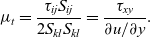 \begin{equation}{\mu _t} = {{{\tau _{ij}}{S_{ij}}} \over {2{S_{kl}}{S_{kl}}}} = {{{\tau _{xy}}} \over {\partial u/\partial y}}.\end{equation}
The extracted distribution of  ${\mu _t}$ can then be used to determine the unknown calibration coefficients,
  ${c_{cr1}}$,
  ${c_{cr2}}$ and
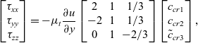
  ${\tilde c_{cr3}}$. By evaluating the diagonal terms of Equation (11) for a parallel mean shear flow, we obtain:
 \begin{equation}\left[ {\begin{array}{*{20}{c}}
{{\tau _{xx}}} \\
{{\tau _{yy}}} \\
{{\tau _{zz}}} \\
\end{array}} \right] = - {\mu _t}\frac{{\partial u}}{{\partial y}}\left[ {\begin{array}{*{20}{c}}
21{1/3} \\
{ - 2}1{1/3} \\
01{ - 2/3} \\
\end{array}} \right]\left[ {\begin{array}{*{20}{c}}
{{c_{cr1}}} \\
{{c_{cr2}}} \\
{{{\tilde c}_{cr3}}} \\
\end{array}} \right],\end{equation}
\begin{equation}\left[ {\begin{array}{*{20}{c}}
{{\tau _{xx}}} \\
{{\tau _{yy}}} \\
{{\tau _{zz}}} \\
\end{array}} \right] = - {\mu _t}\frac{{\partial u}}{{\partial y}}\left[ {\begin{array}{*{20}{c}}
21{1/3} \\
{ - 2}1{1/3} \\
01{ - 2/3} \\
\end{array}} \right]\left[ {\begin{array}{*{20}{c}}
{{c_{cr1}}} \\
{{c_{cr2}}} \\
{{{\tilde c}_{cr3}}} \\
\end{array}} \right],\end{equation}
where  ${\tau _{xx}}$,
  ${\tau _{yy}}$ and
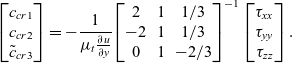
  ${\tau _{zz}}$ correspond to the true normal stresses, which are extracted from DNS. Equation (13) is then inverted to find the values of
  ${c_{cr1}}$,
  ${c_{cr2}}$ and
  ${\tilde c_{cr3}}$ which give the correct normal stresses at each point,
 \begin{equation}\left[ {\begin{array}{*{20}{c}}
{{c_{cr1}}} \\
{{c_{cr2}}} \\
{{{\tilde c}_{cr3}}} \\
\end{array}} \right] = - \frac{1}{{{\mu _t}\frac{{\partial u}}{{\partial y}}}}{\left[ {\begin{array}{*{20}{c}}
21{1/3} \\
{ - 2}1{1/3} \\
01{ - 2/3} \\
\end{array}} \right]^{ - 1}}\left[ {\begin{array}{*{20}{c}}
{{\tau _{xx}}} \\
{{\tau _{yy}}} \\
{{\tau _{zz}}} \\
\end{array}} \right].\end{equation}
\begin{equation}\left[ {\begin{array}{*{20}{c}}
{{c_{cr1}}} \\
{{c_{cr2}}} \\
{{{\tilde c}_{cr3}}} \\
\end{array}} \right] = - \frac{1}{{{\mu _t}\frac{{\partial u}}{{\partial y}}}}{\left[ {\begin{array}{*{20}{c}}
21{1/3} \\
{ - 2}1{1/3} \\
01{ - 2/3} \\
\end{array}} \right]^{ - 1}}\left[ {\begin{array}{*{20}{c}}
{{\tau _{xx}}} \\
{{\tau _{yy}}} \\
{{\tau _{zz}}} \\
\end{array}} \right].\end{equation}
This matrix equation directly determines the constants from the true mean flow and turbulent stresses, which are known from DNS. Equation (14) is then solved at each point for the canonical parallel shear flows described above.
Calibration of (a)  ${c_{cr1}}$, (b)
  ${c_{cr2}}$ and (c)
  ${\tilde c_{cr3}}$ along the wall-normal direction, scaled by the flow thickness,
  ${\delta _{{\rm{ref}}}}$. Flowfields: channel flow (—)(Reference Bernardini, Pirozzoli and Orlandi10,Reference Hoyas and Jiménez11) ; boundary layers (- -)(Reference Sillero, Jiménez and Moser12,Reference Schlatter, Örlü, Li, Brethouwer, Fransson, Johansson, Alfredsson and Henningson13,Reference Schlatter, Li, Brethouwer, Johansson and Henningson14) ; pipe flow (-
 $ \cdot $-)(Reference El Khoury, Schlatter, Noorani, Fischer, Brethouwer and Johansson15).

The values of the coefficients as a function of the wall-normal coordinate, y, are shown in Fig. 1 for the three different parallel mean shear flows. For channel flow and boundary layers, this figure includes data from more than one simulation, as listed in Table 1, in order to represent flows at different Reynolds numbers. Inspection of Fig. 1 suggests that the calibrated coefficients appear to be fairly uniform across much of the flow and are similar between the different flow cases. This finding helps to justify the simplification of assigning the coefficients a single constant value rather than allowing them to vary with non-dimensional wall-normal coordinate. A reasonable value for these coefficients is obtained in three stages. First, the coefficient values between  $y/{\delta _{{\rm{ref}}}} = 0.1$ and
  $1$ are averaged in each data set. The mean of these values is then calculated over the different Reynolds-number cases for each flow field. A final average is then performed over the three canonical flow fields to give calibrated constant coefficient values of
  ${c_{cr1}} = 0.7$,
  ${c_{cr2}} = 2.5$ and
  ${\tilde c_{cr3}} = 0.8$. This modified version of the conventional formulation is termed the ‘extended quadratic constitutive relation’, or extended QCR.
3.1 Effect of eddy-viscosity model on turbulent stress estimates
The effect on turbulent stress estimates of the different eddy-viscosity models, including extended QCR, is studied using the DNS flows listed in Table 1. The estimated turbulent stress distributions are obtained by evaluating the relevant eddy-viscosity model equation using the mean velocities provided by the DNS data and the eddy viscosity,  ${\mu _t}$, from Equation (12). The estimated turbulent stresses are then compared with the ‘true’ values from DNS.
Prior to evaluating the capabilities of extended QCR, conventional eddy-viscosity models are assessed for the cases of channel flow, boundary layers and pipe flow. The turbulent stresses are estimated for: an LEVM which doesn’t account for turbulent kinetic energy (Equation (2)); QCR-2000 (Equation (3)); QCR-2013 (Equation (5)); and an LEVM accounting for turbulent kinetic energy using the  ${c_{cr2}}$ term from QCR-2013 (Equation (6)). Figure 2 shows how the estimated normal stresses (
 ${\tau _{xx}}$,
  ${\tau _{yy}}$ and
  ${\tau _{zz}}$) from each model compare to the distributions from DNS(Reference Bernardini, Pirozzoli and Orlandi10,Reference Sillero, Jiménez and Moser12,Reference El Khoury, Schlatter, Noorani, Fischer, Brethouwer and Johansson15) . This comparison shows that an LEVM based on Equation (2) predicts all three normal stresses to be equal to zero everywhere, which is not an accurate representation of the true distribution.
Effect of different turbulent stress approximations on estimating the normal turbulent stresses (i.  $\overline {{u^{\prime}}{u^{\prime}}} $, ii.
  $\overline {{v^{\prime}}{v^{\prime}}} $, iii.
  $\overline {{w^{\prime}}{w^{\prime}}} $), scaled by the friction velocity,
  ${u_\tau }$. The true stress from DNS (—) and estimated stress from an LEVM (Equation (2), -
 $ \cdot $-), an LEVM with the
  ${c_{cr2}}$ term (Equation (6), -
 $ \cdot $-), QCR-2000 (Equation (3), - -) and QCR-2013 (Equation (5), - -). Flowfields: (a) channel flow(Reference Bernardini, Pirozzoli and Orlandi10); (b) boundary layer(Reference Sillero, Jiménez and Moser12); (c) pipe flow(Reference El Khoury, Schlatter, Noorani, Fischer, Brethouwer and Johansson15). In each case, the stress distributions are presented with the wall-normal coordinate in both outer units (
 $y$) and wall units (
 ${y^ + }$).

From Fig. 2, it is also evident that the  ${c_{cr1}}$ and
  ${c_{cr2}}$ terms in QCR-2013 serve two different purposes. QCR-2000, which contains only the
  ${c_{cr1}}$ term, better predicts the anisotropies between the turbulent stresses, capturing the fact that
  $\overline {{u^{\prime}}{u^{\prime}}} \gt \overline {{w^{\prime}}{w^{\prime}}} \gt \overline {{v^{\prime}}{v^{\prime}}} $. However, the estimated stresses remain much smaller than the true values. On the other hand, the estimates from Equation (6), which contains only the
  ${c_{cr2}}$ term, better estimate the size of the stresses but do not predict any variation between the different turbulent stresses. This observation suggests that the
  ${c_{cr1}}$ term improves prediction of the anisotropy between the normal turbulent stresses, while the
  ${c_{cr2}}$ term improves the estimate of the magnitudes. QCR-2013, which contains both
  ${c_{cr1}}$ and
  ${c_{cr2}}$ terms, therefore benefits from both improvements and features significantly better turbulent stress estimates than the other models. However, even QCR-2013 exhibits noticeable deviations from the true stress distributions, motivating the need for an extended QCR.
A comparison of the turbulent stress estimates from QCR-2013 and extended QCR against the true DNS values is shown in Fig. 3. This figure shows that extended QCR predicts the turbulent stresses substantially better than QCR-2013. Note that these improvements are achieved with coefficient values that are neither spatially dependent nor flow specific. However, in the near-wall region both models struggle to accurately predict the stresses. This observation is particularly evident when the spatial coordinate is scaled in wall units,  ${y^ + }$. These plots show that extended QCR agrees reasonably well with the DNS data in the outer part of the flow but, below
 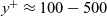 ${y^ + } \approx 100 - 500$, none of the eddy-viscosity models produce satisfactory estimates of the turbulent stresses. Nevertheless, even in this region, extended QCR still generally performs better than the other models.
Effect of different turbulent stress approximations on estimating the normal turbulent stresses (i.  $\overline {{u^{\prime}}{u^{\prime}}} $, ii.
  $\overline {{v^{\prime}}{v^{\prime}}} $, iii.
  $\overline {{w^{\prime}}{w^{\prime}}} $), scaled by the friction velocity,
  ${u_\tau }$. The true stress from DNS (—) and estimated stress from QCR-2013 (Equation (5), - -) and extended QCR (Equation (11), —). Flowfields: (a) channel flow(Reference Bernardini, Pirozzoli and Orlandi10); (b) boundary layer(Reference Sillero, Jiménez and Moser12); (c) pipe flow(Reference El Khoury, Schlatter, Noorani, Fischer, Brethouwer and Johansson15). In each case, the stress distributions are presented with the wall-normal coordinate in both outer units (
 $y$) and wall units (
 ${y^ + }$).
Effect of Reynolds number on estimates of normal turbulent stresses (i.  $\overline {{u^{\prime}}{u^{\prime}}} $, ii.
  $\overline {{v^{\prime}}{v^{\prime}}} $, iii.
  $\overline {{w^{\prime}}{w^{\prime}}} $), scaled by the friction velocity,
  ${u_\tau }$. The true stress from DNS (—) and estimated stress from QCR-2013 (Equation (5), - -) and extended QCR (Equation (11), —). Reynolds numbers: (a) Re
 $_\tau $ = 2,050; (b) Re
 $_\tau $ = 1,000; (c) Re
 $_\tau $ = 550; (d) Re
 $_\tau $ = 180(Reference Bernardini, Pirozzoli and Orlandi10). In each case, the stress distributions are presented with the wall-normal coordinate in wall units (
 ${y^ + }$), with the data in outer units (
 $y$) only included for cases (a) and (d) for brevity.

The poor predictions in the near-wall region can be attributed to the fact that extended QCR has been developed in free shear flows and does not take advantage of any information regarding the proximity of the wall. Capturing this wall-normal dependence remains a challenge for the future, perhaps using the approach of QCR-2020, which allows the values of coefficients to vary with wall-normal distance. It is worth noting, however, that even QCR-2020 has trouble reproducing, in particular, the sharp near-wall peak of  ${\tau _{xx}}$ at high Reynolds numbers(Reference Rumsey, Carlson, Pulliam and Spalart20).
In addition to evaluating the improvement in turbulent stress estimates by extended QCR for different flow fields, it is also useful to consider the effects of Reynolds number. This analysis is performed using the channel flow as an example, which was studied for Re $_\tau = 4100$ in Fig. 3(a). However, DNS simulations were also conducted by Bernardini et al. for the same flow field at Re
 $_\tau = 2050$, 1000, 550, and 180. Figure 4 presents the turbulent stresses from the velocity statistics for these additional simulations, alongside the estimated distributions from QCR-2013 and extended QCR. This comparison shows that extended QCR provides a better estimate of the normal stresses than QCR-2013, not just at Re
 $_\tau = 4100$ where the coefficient values were calibrated, but for the entire Reynolds-number range, Re
 $_\tau = 180$ – 4100.
A similar analysis to the parallel mean shear flows in Fig. 3 can also be extended to the more complex cases in Table 1, namely the separated boundary layer(Reference Coleman, Rumsey and Spalart16) and the flow in a square duct(Reference Pirozzoli, Modesti, Orlandi and Grasso17). In contrast to the parallel shear flows from Fig. 3, the mean velocity in such flow fields (which have non-zero cross-flow and which vary in x or z) are no longer determined solely by  ${\tau _{xy}}$. Therefore, it is not possible to use the eddy-viscosity distribution from Equation (12) to correctly relate shear stress with the mean flow. Instead, a different method is used to evaluate a relevant eddy-viscosity distribution,
  ${\mu _t}$, which provides the best fit for a weighted balance of all six turbulent stress components:
 \begin{equation} {{\mu _t} = \frac{{\tau _{ij}}{{\tilde \sigma }_{ij}}}{{{\tilde \sigma }_{kl}}{{\tilde \sigma }_{kl}}}}. \end{equation}
In this equation,  ${\tau _{ij}}$ is the true turbulent stress tensor from DNS and
  ${\tilde \sigma _{ij}} = {\tilde \tau _{ij}}$ /
  ${\mu _t}$, where the definition of
  ${\tilde \tau _{ij}}$ is taken from Equations (5) or (11) for QCR-2013 and extended QCR, respectively. Note that
  ${\tilde \tau _{ij}}$ is proportional to
  ${\mu _t}$ for all three definitions, and so
  ${\tilde \sigma _{ij}}$ is independent of
  ${\mu _t}$.
Figure 5 shows the estimated normal turbulent stresses ( ${\tau _{xx}}$,
  ${\tau _{yy}}$ and
  ${\tau _{zz}}$) for these flows. This figure exhibits similar behaviour to that from the simpler flow cases (Fig. 3). In the outer part of the flow, extended QCR provides substantial improvements compared to QCR-2013. However, whilst the turbulent stresses appear to be reasonably predicted down to
  ${y^ + } = 10$ for the separated boundary layer, neither of the eddy-viscosity models provide accurate estimates for the turbulent stresses in the near-wall region (
 ${y^ + } \mathbin{\lower.3ex\hbox{$\buildrel \lt \over{\smash{\scriptstyle\sim}\vphantom{_x}}$}} 60$) of the corner bisector for the square duct flow. This finding further highlights the importance of capturing the wall-normal dependency of the QCR coefficients in future improvements to the current model.
Effect of different turbulent stress approximations on estimating the normal turbulent stresses (i.  $\overline {{u^{\prime}}{u^{\prime}}} $, ii.
  $\overline {{v^{\prime}}{v^{\prime}}} $, iii.
  $\overline {{w^{\prime}}{w^{\prime}}} $), scaled by the bulk velocity,
  ${u_b}$. The true stress from DNS (—) and estimated stress from QCR-2013 (Equation (5), - -) and extended QCR (Equation (11), —). Flowfields: (a) separated boundary layer(Reference Coleman, Rumsey and Spalart16); (b) corner bisector of duct flow(Reference Pirozzoli, Modesti, Orlandi and Grasso17). In each case, the stress distributions are presented with the wall-normal coordinate in both outer units (
 $y$) and wall units (
 ${y^ + }$).

Figures 3 and 5, therefore, suggest that extended QCR improves the predictions of turbulent stresses, which might be expected to improve the calculation of mean flow fields. In order to test the effect on mean flow behaviour, it would be necessary to assess the accuracy of RANS simulations conducted using extended QCR. Such an assessment is outside the scope of the present paper but would be the ultimate test of the proposed quadratic eddy-viscosity model.
4.0 Prediction of corner flows using qcr
The analysis of DNS data in Figs. 3 and 5 has shown that QCR-2013 produces a somewhat inaccurate estimate of turbulent stresses. Nevertheless, conventional QCR appears to more accurately calculate the flow along corner geometries than the corresponding linear eddy-viscosity models(Reference Mani, Babcock, Winkler and Spalart4,Reference Bisek5,Reference Dandois7) . The successful prediction of stress-induced corner vortices using poor estimates of the turbulent stresses is somewhat counter-intuitive. In order to better understand this apparent contradiction, the turbulent stresses in corner flows are analysed more closely.
4.1 Analysis of turbulent stresses
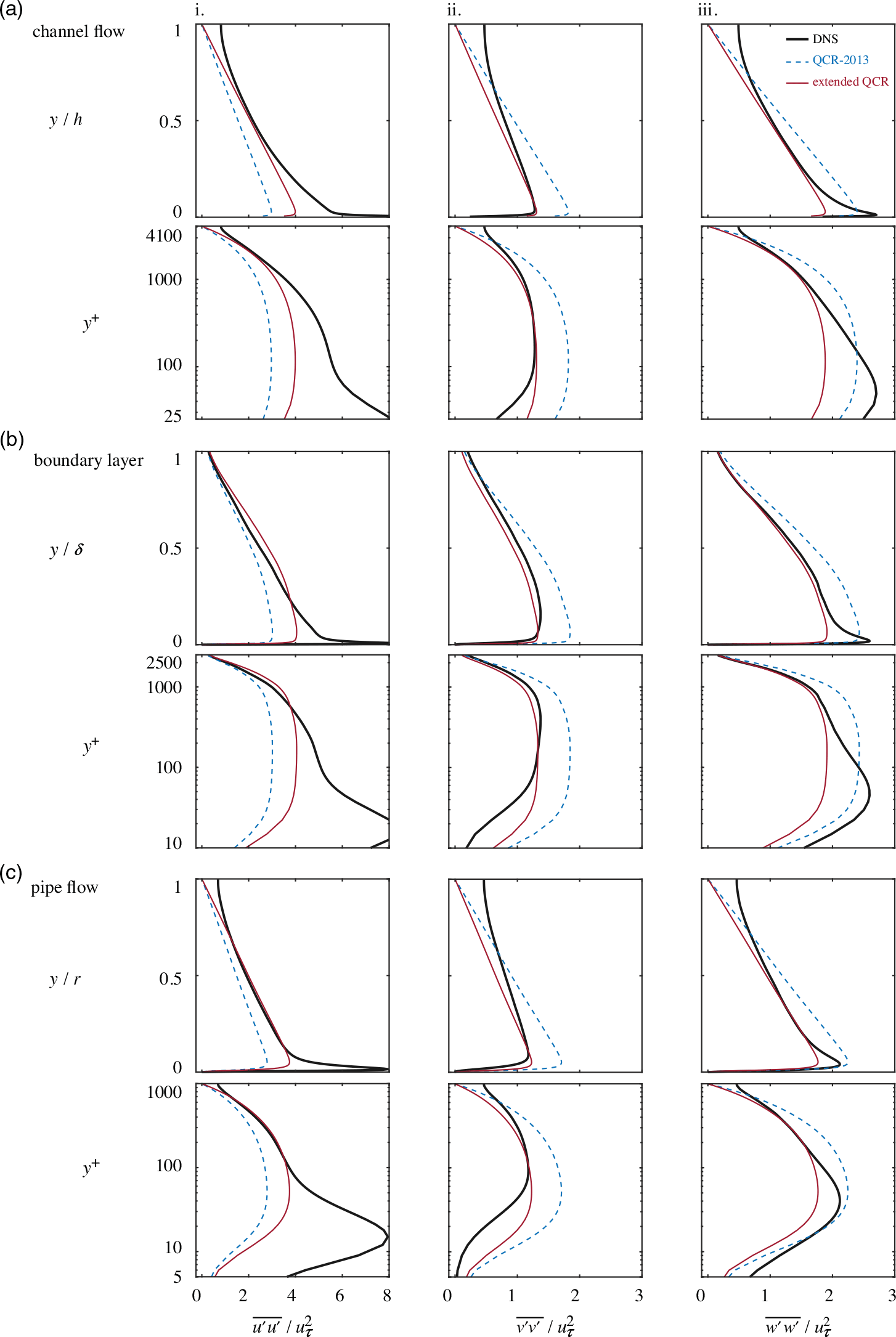
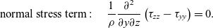
Since corner flows are dominated by the presence of a counter-rotating pair of streamwise vortices(Reference Gessner and Jones1), we consider the mean streamwise vorticity equation:
 \begin{align} v{{\partial {\omega _x}} \over {\partial y}} + w{{\partial {\omega _x}} \over {\partial z}} = \underbrace {{\omega _y}{{\partial u} \over {\partial y}} + {\omega _z}{{\partial u} \over {\partial z}}}_{\rm{A}} & + \underbrace {\nu \left( {{{{\partial ^2}} \over {\partial {y^2}}} + {{{\partial ^2}} \over {\partial {z^2}}}} \right){\omega _x}}_{\rm{B}} \nonumber\\
& + \underbrace {\left( {{{{\partial ^2}} \over {\partial {y^2}}} - {{{\partial ^2}} \over {\partial {z^2}}}} \right)\left( { - \overline {v^{\prime}w^{\prime}} } \right)}_{\rm{C}} + \underbrace {{{{\partial ^2}} \over {\partial y\partial z}}\left( {\overline {{{v^{\prime}}^2}} - \overline {{{w^{\prime}}^2}} } \right)}_{\rm{D}}, \end{align}
\begin{align} v{{\partial {\omega _x}} \over {\partial y}} + w{{\partial {\omega _x}} \over {\partial z}} = \underbrace {{\omega _y}{{\partial u} \over {\partial y}} + {\omega _z}{{\partial u} \over {\partial z}}}_{\rm{A}} & + \underbrace {\nu \left( {{{{\partial ^2}} \over {\partial {y^2}}} + {{{\partial ^2}} \over {\partial {z^2}}}} \right){\omega _x}}_{\rm{B}} \nonumber\\
& + \underbrace {\left( {{{{\partial ^2}} \over {\partial {y^2}}} - {{{\partial ^2}} \over {\partial {z^2}}}} \right)\left( { - \overline {v^{\prime}w^{\prime}} } \right)}_{\rm{C}} + \underbrace {{{{\partial ^2}} \over {\partial y\partial z}}\left( {\overline {{{v^{\prime}}^2}} - \overline {{{w^{\prime}}^2}} } \right)}_{\rm{D}}, \end{align}
where  ${\omega _x}$,
  ${\omega _y}$ and
  ${\omega _z}$ are the vorticity components in the streamwise, wall-normal and spanwise directions, while
  $\nu $ is the kinematic viscosity of the flow. This equation shows the balance of the convection of vorticity (the left side) with production and diffusion on the right side. Term A on the right side corresponds to the generation of Prandtl vortices of the first kind, corresponding to a bending of vortex lines by the mean shear. The second term (B) represents the viscous diffusion of vorticity. The third and fourth terms (C and D) correspond to the production of Prandtl vortices of the second kind, which is related to turbulent stress anisotropy in the flow.
The streamwise vortices which exist in corner flows are believed to be generated by mechanisms relating to Prandtl vortices of the second kind(Reference Gessner and Jones1), corresponding to terms C and D above. We therefore restrict our attention to these two terms, which are referred to as the ‘shear stress term’ (term C) and the ‘normal stress term’ (term D). These two terms are evaluated using the turbulent stresses estimated using an LEVM, QCR-2013 and extended QCR, and are then compared with the equivalent ‘correct’ distribution calculated from the DNS turbulent stresses.
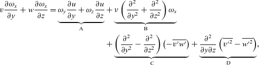
For this analysis, we assume that in corner flows the streamwise velocities are much greater than any transverse velocity components ( $v \approx w \approx 0$) and the flow is fully developed (
 $\partial u/\partial x = 0$). For a linear eddy-viscosity model, defined by Equation (6), we find that
  ${\tau _{yz}} = 0$ and
  ${\tau _{yy}} = {\tau _{zz}}$, which gives:
 \begin{equation}{\rm{shear\ stress\ term}}:\quad {1 \over \rho }\left( {{{{\partial ^2}} \over {\partial {y^2}}} - {{{\partial ^2}} \over {\partial {z^2}}}} \right){\tau _{yz}} = 0,\end{equation}
 \begin{equation}{\rm{normal\ stress\ term}}:\quad {1 \over \rho }{{{\partial ^2}} \over {\partial y\partial z}}\left( {{\tau _{zz}} - {\tau _{yy}}} \right) = 0.\end{equation}
Since the vorticity production terms equate to zero, RANS simulations with an LEVM are unable to generate the quasi-streamwise vortices that exist in corners, resulting in a poor prediction of these flows.
The situation is different when quadratic modifications are introduced, however. Rather than repeating the entire analysis separately for QCR-2013 and extended QCR, both models can be studied simultaneously using Equation (11). As determined in Section 3.0, the proposed values of  ${c_{cr1}} = 0.7$,
  ${c_{cr2}} = 2.5$ and
  ${\tilde c_{cr3}} = 0.8$ give extended QCR. On the other hand, QCR-2013, which does not contain the
  ${\tilde c_{cr3}}$ term, can be replicated by using Equation (11) with the coefficient combination
  ${c_{cr1}} = 0.3$,
  ${c_{cr2}} = 2.5$ and
  ${\tilde c_{cr3}} = 0$. Evaluating the relevant turbulent stress combinations for the shear stress term and the normal stress term in Equation (16) for a corner flow,
  $u\left( {y,z} \right)$, we find that:
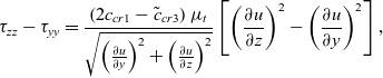 \begin{equation}\tau _{zz} - \tau _{yy} = \frac{\left( {2{c_{cr1}} - {{\tilde c}_{cr3}}} \right){\mu _t}}{\sqrt{{\left( \frac{\partial u}{\partial y} \right)}^2 + {\Big( \frac{\partial u}{\partial z} \Big)}^2 }}
\left[ {{{\left( {{\frac{\partial u}{\partial z}}} \right)}^2} - {{\left( {{\frac{\partial u}{\partial y}}} \right)}^2}} \right],\end{equation}
\begin{equation}\tau _{zz} - \tau _{yy} = \frac{\left( {2{c_{cr1}} - {{\tilde c}_{cr3}}} \right){\mu _t}}{\sqrt{{\left( \frac{\partial u}{\partial y} \right)}^2 + {\Big( \frac{\partial u}{\partial z} \Big)}^2 }}
\left[ {{{\left( {{\frac{\partial u}{\partial z}}} \right)}^2} - {{\left( {{\frac{\partial u}{\partial y}}} \right)}^2}} \right],\end{equation}
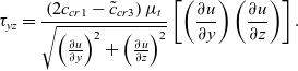 \begin{equation}{\tau _{yz}} = {\frac{\left( {2{c_{cr1}} - {{\tilde c}_{cr3}}} \right){\mu _t}}{\sqrt {{{\left( {{\frac{\partial u}{\partial y}}} \right)}^2} + {\Big( \frac{\partial u}{\partial z} \Big)}^2} }}
\left[ {\left( {{\frac{\partial u}{\partial y}}} \right)\left( {{\frac{\partial u}{\partial z}}} \right)} \right].\end{equation}
\begin{equation}{\tau _{yz}} = {\frac{\left( {2{c_{cr1}} - {{\tilde c}_{cr3}}} \right){\mu _t}}{\sqrt {{{\left( {{\frac{\partial u}{\partial y}}} \right)}^2} + {\Big( \frac{\partial u}{\partial z} \Big)}^2} }}
\left[ {\left( {{\frac{\partial u}{\partial y}}} \right)\left( {{\frac{\partial u}{\partial z}}} \right)} \right].\end{equation}
These turbulent stress combinations only depend on the constant combination  $2{c_{cr1}} - {\tilde c_{cr3}}$. This suggests that the generation of streamwise vorticity depends only on the value of
  $2{c_{cr1}} - {\tilde c_{cr3}}$ (i.e. some measure of the strength of the quadratic modification) rather than the individual contributions from the different terms. Therefore, while corner flows do show the importance of quadratic terms in turbulence modelling, they are poor at discriminating between them. The dependence of vorticity production on
  $2{c_{cr1}} - {\tilde c_{cr3}}$ suggests that, if the combined use of both (or all three) quadratic terms can generate accurate stresses, the streamwise vorticity in corner flows can be produced using just one of these terms, such as in conventional QCR. For this to be the case, it is necessary that the model which provides accurate stress estimates and conventional QCR both share a common value of
  $2{c_{cr1}} - {\tilde c_{cr3}}$.
Indeed, it is interesting to note that  $2{c_{cr1}} - {\tilde c_{cr3}} = 0.6$ both for QCR-2013 and for extended QCR. This suggests that vorticity production in corner flows is essentially equivalent between the two forms and provides an explanation for the success of conventional QCR in such flows despite somewhat poor turbulent stress prediction. An additional consequence of this finding is that extending QCR to its more general form is unlikely to detrimentally impact the key success of conventional QCR, i.e. the prediction of the mean flow along streamwise corners.
4.2 Analysis of velocity statistics from DNS
Data from relevant direct numerical simulations are used to illustrate the findings from Section 4.1. A fully developed, incompressible square duct flow was computed by Pirozzoli et al. for a friction Reynolds number, Re $_\tau = 1100$(Reference Pirozzoli, Modesti, Orlandi and Grasso17). Figures 6(a) and (b) show the streamwise velocity and vorticity distributions, respectively, for a quarter of the duct. As well as capturing the shear in the boundary layers, the vorticity distribution displays the pair of counter-rotating vortices (labelled V+ and V−) either side of the corner bisector. The distorted boundary-layer shape, denoted by the dotted line in Fig. 6(a), demonstrates how the vortices affect the streamwise velocity profile through momentum transfer between the core flow and the boundary layers.
Direct numerical simulation of the flow in a quarter of a square duct(Reference Pirozzoli, Modesti, Orlandi and Grasso17) with half-height,  $h$, and bulk velocity,
  ${u_b}$: (a) the mean streamwise velocity component,
  $u$, with the highlighted contour at
  $u$/
$u$/ ${u_b} = 1$, representative of the boundary-layer edge shape; (b) the mean streamwise vorticity,
  ${\omega _x}$. Contours of positive values are shown with solid lines and negative values are marked by dashed lines.

Figure 7(a) presents the turbulent stresses ( ${\tau _{yz}}$,
  ${\tau _{yy}}$ and
  ${\tau _{zz}}$) that appear in the streamwise vorticity equation (Equation (16)), extracted directly from DNS. The turbulent shear stress,
  $\overline {{u^{\prime}}{v^{\prime}}} $, is negative along the corner bisector and is roughly zero on either side. The normal stresses are generally larger in magnitude than the shear stress, with
  $\overline {{v^{\prime}}{v^{\prime}}} $ concentrated towards the floor and
  $\overline {{w^{\prime}}{w^{\prime}}} $ towards the sidewall. These distributions are compared with equivalent estimates using Equations (6), (5) and (11), which correspond to an LEVM, QCR-2013 and extended QCR, respectively.
Turbulent stresses relevant for streamwise vorticity production, in the square duct(Reference Pirozzoli, Modesti, Orlandi and Grasso17): i.  $\overline {{u^{\prime}}{v^{\prime}}} $, ii.
  $\overline {{v^{\prime}}{v^{\prime}}} $ and iii.
  $\overline {{w^{\prime}}{w^{\prime}}} $. These stresses are (a) directly extracted from the DNS turbulence statistics, or are estimated using (b) a linear eddy-viscosity model, (c) QCR-2013, and (d) extended QCR. Contours of positive values are shown with solid lines and negative values are marked by dashed lines.

A comparison of Fig. 7(a) with (b) shows that linear eddy-viscosity models cannot accurately predict the distribution of relevant turbulent stresses. When the QCR-2013 modification is used, there is an improvement in  ${\tau _{yz}}$ (Fig. 7(c–i)), which now more closely reflects the distribution in Fig. 7(a–i). However, the estimates of
  ${\tau _{yy}}$ (Fig. 7(c–ii)) and
  ${\tau _{zz}}$ (Fig. 7(c–iii)) are still inaccurate in both magnitude and topology. Figure 7(d) shows that extended QCR appears to provide a reasonable prediction of all three stresses, although the true stress distributions from Fig. 7(a) are still not perfectly replicated.
As well as investigating the individual turbulent stresses, Fig. 8 shows the equivalent comparison for the stress combination  ${\tau _{zz}} - {\tau _{yy}}$, which appears in the normal stress term of Equation (16). Linear eddy-viscosity models that obey Equation (6) assume that
  ${\tau _{yy}} = {\tau _{zz}}$, and so the difference between the two stress components evaluates to zero. Since this distribution would correspond to an empty plot, it is not shown in Fig. 8. More interestingly, Fig. 8(b) and (c) appear to be equivalent, which shows that QCR-2013 exactly emulates the estimates from extended QCR. This is a direct consequence of the finding in Section 4.1 that, for these quadratic modifications,
  ${\tau _{zz}} - {\tau _{yy}}$ depends only on
  $2{c_{cr1}} - {\tilde c_{cr3}}$. This coefficient combination evaluates to 0.6 for both QCR-2013 and extended QCR. For the same reason, the distribution of
  ${\tau _{yz}}$ in Fig. 7(c–i) (QCR-2013) and Fig. 7(d–i) (extended QCR) appear to be equivalent.
Turbulent stress combination  $\overline {{w^{\prime}}{w^{\prime}}} - \overline {{v^{\prime}}{v^{\prime}}} $, in the square duct(Reference Pirozzoli, Modesti, Orlandi and Grasso17). These terms are (a) directly extracted from the DNS turbulence statistics, or are estimated using (b) QCR-2013 and (c) extended QCR. Contours of positive values are shown with solid lines and negative values are marked by dashed lines. Note that the equivalent plot for an LEVM is blank and so has not been presented here.

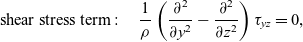
From the turbulent stress distributions, the shear stress and the normal stress terms from Equation (16) are evaluated, both individually and in combination (Fig. 9). Figure 9(a) presents these vorticity production terms for the DNS stress distributions. The overall vorticity production (Fig. 9(a–iii)) takes the form of one lobe each side of the corner bisector (P $^ + $ and P
 $^ - $), with opposite sign. Both production terms affect these lobes, with the shear stress term contributing more towards the corner bisector and the normal stress term influencing the behaviour close to the walls.
The streamwise vorticity production terms from Equation (16), in the square duct(Reference Pirozzoli, Modesti, Orlandi and Grasso17): i. shear stress term  $\left( {{h^2}/u_b^2\left( {{\partial ^2}/\partial {y^2} - {\partial ^2}/\partial {z^2}} \right)\left( { - \overline {v^{\prime}w^{\prime}} } \right)} \right)$, ii. normal stress term
 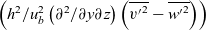 $\left( {{h^2}/u_b^2\left( {{\partial ^2}/\partial y\partial z} \right)\left( {\overline {{{v^{\prime}}^2}} - \overline {{{w^{\prime}}^2}} } \right)} \right)$, and iii. sum of shear stress term and normal stress term. These terms are (a) directly extracted from the DNS turbulence statistics, or are estimated using (b) QCR-2013 and (c) extended QCR. Contours of positive values are shown with solid lines and negative values are marked by dashed lines. Note that the equivalent plot for an LEVM is blank and so has not been presented here.

As expected from the analysis of the streamwise vorticity equation, the vorticity production terms for LEVMs evaluate to zero, so such models cannot produce streamwise vorticity using this mechanism. Since this distribution would produce an empty contour plot, it is not included in Fig. 9. The production terms for QCR-2013 (Fig. 9(c)) and extended QCR (Fig. 9(d)) produce very similar distributions to one another. This is a consequence of these two quadratic modifications displaying equivalent spatial distributions for the relevant turbulent stress combinations  ${\tau _{yz}}$ (Figs. 7(c–i) and (d–i)) and
  ${\tau _{zz}} - {\tau _{yy}}$ (Fig. 8(b) and (c)). Therefore, the following discussion does not distinguish between QCR-2013 and extended QCR.
A closer analysis of Fig. 9 shows that the estimated vorticity production for QCR exhibits primary lobes of the correct sign. These are labelled P $_1^ + $ and P
 $_1^ - $, corresponding to P
 $^ + $ and P
 $^ - $ from Fig. 9(a). This rough agreement in the structure, sign and magnitude of the production terms explains the improvement in simulation of corner flows when QCR is used.
However, the topology of the production terms for the quadratic models do exhibit deviations from the ‘true’ DNS distribution. A direct comparison of Fig. 9(b–i) and (c-i) to Fig. 9(a–i) shows that QCR underestimates the contribution from the shear stress term. Instead, the primary lobes in the quadratic models (P $_1$) are determined mainly from the normal stress term. As a result, the estimate of overall vorticity production by QCR (Fig. 9(b-iii) and (c–iii)) does not correspond well with the true distribution (Fig. 9(a–iii)). In particular, QCR predicts the P
 $_1$ lobes to be elongated close to the corner bisector whilst the true production distribution (P
 $^ + $ and P
 $^ - $) is concentrated towards the walls. This suggests that, whereas QCR is able to predict the presence of corner vortices and the resultant boundary-layer shape, the properties of the vortices (such as their position) may not quite correspond to those in the physical flow.
Another reported limitation of QCR in corner flows occurs when simulations are run with  ${c_{cr1}}$ greater than the recommended value of 0.3, which may occur, for example, in an attempt to better match the mean flow. In such cases, additional non-physical vortices are generated(Reference Leger, Bisek and Poggie8). To investigate this phenomenon further, the vorticity production terms are estimated for
  ${c_{cr1}} = 0.5$ and
  ${\tilde c_{cr3}} = 0$, i.e.
  $2{c_{cr1}} - {\tilde c_{cr3}} = 1.0$ rather than 0.6. The primary effect is to strengthen all the turbulent stresses and thus increase the overall vorticity production, shown in Fig. 10(c). This figure also reveals the appearance of additional lobes away from the corner bisector, labelled P
 $_2^ + $ and P
 $_2^ - $. These lobes are of opposite sign to the primary P
 $_1$ lobes. The P
 $_2$ lobes also appear in Fig. 10(a), and so seem to be associated with the shear stress term in Equation (16). Note that weak analogues to these P
 $_2$ lobes can be identified in Fig. 9(b–iii) and (c–iii), where
  $2{c_{cr1}} - {\tilde c_{cr3}} = 0.6$. The lobes in Fig. 10, however, are strong enough to be prominent in the distribution of overall vorticity production. The presence of the P
 $_2$ lobes may correspond to the non-physical vortices reported in RANS simulations of these geometries(Reference Leger, Bisek and Poggie8).
The streamwise vorticity production terms from Equation (16), in the square duct(Reference Pirozzoli, Modesti, Orlandi and Grasso17): (a) shear stress term  $\left( {{h^2}/u_b^2\left( {{\partial ^2}/\partial {y^2} - {\partial ^2}/\partial {z^2}} \right)\left( { - \overline {v^{\prime}w^{\prime}} } \right)} \right)$, (b) normal stress term
  $\left( {{h^2}/u_b^2\left( {{\partial ^2}/\partial y\partial z} \right)\left( {\overline {{{v^{\prime}}^2}} - \overline {{{w^{\prime}}^2}} } \right)} \right)$, and (c) sum of shear stress term and normal stress term. These terms are obtained with
  ${c_{cr1}} = 0.5$,
  ${c_{cr2}} = 2.5$ and
  ${\tilde c_{cr3}} = 0$ in Equation (11). Contours of positive values are shown with solid lines and negative values are marked by dashed lines.
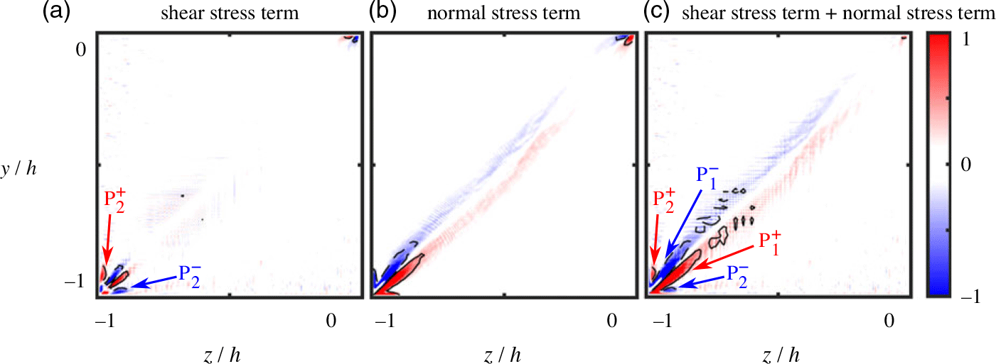
In this way, the appearance of the spurious vortices can be linked to the shear stress term in Equation (16) and, in turn, the inaccuracy of estimating the turbulent shear stress component,  ${\tau _{yz}}$. However, the dependence of the production terms only on the combination
  $2{c_{cr1}} - {\tilde c_{cr3}}$ suggests that any simple quadratic modification would face similar issues with corner flow prediction. To overcome this, it is necessary to add complexity either by capturing the wall-normal dependence of the coefficients or by estimating the turbulent stresses using a different, more involved technique.
5.0 Conclusions
This paper revisits the quadratic constitutive relation, a modification to linear eddy-viscosity models. The analysis in this paper shows that the conventional form of QCR provides a definite improvement but does not, in general, compute the turbulent stresses very accurately, which may help to explain why its success in mean flow prediction for many flow fields has been limited.
The improvements in computing the flow along streamwise corners reported by others are not due to a much better prediction of turbulent stresses in general. Instead, this success can be attributed to improved estimates of the particular turbulent stress combinations which appear in the mean streamwise vorticity equation. As a result, the topology and rough magnitudes of the vorticity production terms are in reasonable agreement with the true values from DNS, which explains why corner flow computations are improved. Nevertheless, the precise topology of the production terms deviates from the DNS distribution, particularly close to the walls, which suggests that the properties of the vortices (such as their position) may not quite correspond to those in the physical flow. In addition, the imperfect estimate of the shear stress term is observed to be the source of additional, non-physical vortices when the QCR coefficient,  ${c_{cr1}}$, exceeds 0.3.
An extension to QCR is proposed, which improves turbulent stress predictions over a wide range of canonical and more complex flows. For a small increase in complexity, with one additional quadratic modification term and associated coefficient compared to QCR, the turbulent stress estimates now match the true values from DNS more closely. The flow along streamwise corner geometries is one such example of a flow field where extended QCR predicts turbulent stresses with reasonable accuracy. It turns out that streamwise vorticity production in such flows depends only on the coefficient combination  $2{c_{cr1}} - {\tilde c_{cr3}}$ rather than the precise values of each coefficient. The fact that both extended QCR and conventional QCR have
  $2{c_{cr1}} - {\tilde c_{cr3}} = 0.6$ explains why conventional QCR can reliably predict the generation of corner vortices despite inaccurate turbulent stress estimates. This finding also implies that, whilst corner flow calculations are affected by the presence of quadratic terms in the eddy-viscosity model, this flow field is not a suitable test case for comparing the capabilities of different quadratic models.
Note that the proposed formulation of extended QCR is still not perfect, however. In particular, the stresses near the wall are still poorly predicted, demanding a closer study into the wall-normal dependence of this type of model. Nevertheless, the marked improvement in turbulent stress predictions is promising and provides compelling reasons to conduct RANS simulations with extended QCR. These computations would enable the effect of the proposed modification on mean flow calculations to be assessed. Such calculations would also permit evaluation of the numerical stability of this modification, and would test the existence of possible spurious vortices in a model where  ${c_{cr1}} = 0.7$ greatly exceeds 0.3.
Acknowledgements
This material is based upon work supported by the US Air Force Office of Scientific Research under award FA9550–16–1–0430.
Supplementary Material
For supplementary material accompanying this paper visit https://doi.org/10.1017/aer.2021.42


 Open access