


Introduction
Mass loss from outlet glaciers in Antarctica is a primary source of uncertainty in sea-level rise projections (Cornford and others, Reference Cornford2015; DeConto and Pollard, Reference DeConto and Pollard2016). A prerequisite to reliable projections of mass loss from Antarctica is understanding what sets the flow speed of ice streams and outlet glaciers. The driving force of ice streams is gravity, due to the sloped topography of the ice surface. However, the resisting forces of ice flow in ice streams are not fully constrained in Antarctica, and this contributes to the uncertainty of the response of outlet glaciers to changes in climate.
The flow of ice streams is resisted in part by drag at the bed (Echelmeyer and others, Reference Echelmeyer, Harrison, Larsen and Mitchell1994), commonly related to the basal velocity through a sliding law. A typical form of the sliding law, and the form taken in this study, relates the basal drag to a power of the basal velocity with a prefactor denoted here as basal slipperiness (Weertman, Reference Weertman1957). Basal drag represents resistance to slip at the ice–bed interface, and so basal slipperiness represents the lack of resistance to slip at the ice–bed interface. Inversions for the sliding-law prefactor in ice streams in Antarctica suggest that the prefactor in the sliding law can vary spatially and temporally over a wide range of values due to variations in bed composition, roughness, and water pressure (Joughin and others, Reference Joughin, MacAyeal and Tulaczyk2004; Morlighem and others, Reference Morlighem, Seroussi, Larour and Rignot2013; Isaac and others, Reference Isaac, Petra, Stadler and Ghattas2015).
The flow of ice streams is also constrained by viscous forces within the ice. On long timescales, ice flows as a non-Newtonian fluid with a viscosity that is a function of strain rate and a flow-rate parameter (the prefactor in the constitutive relation). The flow-rate parameter depends on ice temperature, crystal size and orientation, porosity, interstitial liquid water content, and the density of the ice, among other factors (Cuffey and Paterson, Reference Cuffey and Paterson2010). These dependencies suggest that the flow-rate parameter is not constant in space or time, as deformation softens the ice through viscous dissipation and evolution of the crystalline structure, further affecting deformation rates (Alley, Reference Alley1988; Jacobson and Raymond, Reference Jacobson and Raymond1998; Minchew and others, Reference Minchew, Meyer, Robel, Gudmundsson and Simons2018).
Previous studies have used inverse methods to infer basal drag or the flow-rate parameter from suites of observations. Inverse methods are a class of methods that use observations to infer parameters of a model. The classical inverse method involves the construction of a cost function and a subsequent optimization step to minimize the misfit between the output of a model and the observations (MacAyeal, Reference MacAyeal1993). The inversions done to infer basal properties and properties of ice rheology make use of surface velocity data, relying on the fact that basal drag and ice rheology affect surface velocity. These inverse methods also require estimates of ice thickness, surface elevation, and ice density. Gudmundsson (Reference Gudmundsson2003) as well as Raymond and Gudmundsson (Reference Raymond and Gudmundsson2005) describe the effect of basal properties on surface velocity and topography, suggesting that surface velocity datasets, along with surface topography and ice thickness data, might be sufficient to infer basal properties (basal drag and basal topography). A later study confirmed that accurate inferences of basal properties can be achieved using surface velocity and topography data (Gudmundsson and Raymond, Reference Gudmundsson and Raymond2008).
Initial studies conducted inversions to infer a single parameter, assuming that other parameters are known (MacAyeal, Reference MacAyeal1992, Reference MacAyeal1993; MacAyeal and others, Reference MacAyeal, Bindschadler and Scambos1995; Larour and others, Reference Larour, Rignot, Joughin and Aubry2005; Morlighem and others, Reference Morlighem2010, Reference Morlighem, Seroussi, Larour and Rignot2013; Habermann and others, Reference Habermann, Maxwell and Truffer2012). However, there are uncertainties in multiple parameters that are not incorporated into these single inversions. In particular, both basal drag and the flow-rate parameter are unknown parameters. Assuming one is known introduces errors into the single inversion. Since both basal slip and ice rheology act as controls on the speed of flow, inferring both basal friction and the flow-rate parameter simultaneously is necessary (Arthern and others, Reference Arthern, Hindmarsh and Williams2015).
Previous studies have resolved multiple parameters using inverse methods. Gudmundsson and Raymond (Reference Gudmundsson and Raymond2008) used surface topography and surface velocity data to estimate basal topography and the basal drag coefficient using a Bayesian inverse method. Raymond and Gudmundsson (Reference Raymond and Gudmundsson2009) conducted the same Bayesian inversion through the use of nonlinear optimization and transfer functions. Perego and others (Reference Perego, Price and Stadler2014) inferred the basal slipperiness coefficient and basal topography using adjoint-based optimization for model initialization. Other studies have inverted for basal drag and the flow-rate parameter. Arthern (Reference Arthern2015) and Arthern and others (Reference Arthern, Hindmarsh and Williams2015) performed this inversion using Bayesian methods and iterative methods with regularization. Arthern and Gudmundsson (Reference Arthern and Gudmundsson2010) inverted for viscosity and basal drag to initialize ice flow models. Cornford and others (Reference Cornford2015) inferred a coefficient of ice viscosity and basal drag for large-scale ice-sheet simulations. Hoffman and others (Reference Hoffman2018) implemented inversions for viscosity and basal drag following Perego and others (Reference Perego, Price and Stadler2014) in a land-ice model. Finally, Gudmundsson and others (Reference Gudmundsson, Paolo, Adusumilli and Fricker2019) inferred basal slipperiness and the flow-rate parameter, in a similar method used here, over Antarctica to estimate mass loss due to the ice shelf thinning.
While these joint inversions have been accomplished using surface velocity data, no study has yet examined the performance and accuracy of jointly inferring the flow-rate parameter and basal drag. To date, it has been unclear whether it is possible to separate the effects of these two parameters while inferring both parameters in the same spatial location from a single dataset (Habermann and others, Reference Habermann, Maxwell and Truffer2012; Arthern, Reference Arthern2015). In this study, we introduce a new approach that incorporates strain rates into the regularization to minimize any mixing between the two parameters in the inversion. We use synthetic experiments designed to resemble natural ice streams to determine how accurate these methods are in terms of constraining both the magnitude and the distribution of the slipperiness coefficient and flow-rate parameter. After showing that the inferred values agree with the true value, we apply our inversion method to data collected over Bindschadler and MacAyeal Ice Streams, West Antarctica.
Model and inverse method
For this study, surface velocities are modeled using a finite-element ice flow model Úa, which solves the shallow-shelf approximation (SSA; Gudmundsson and others, Reference Gudmundsson, Krug, Durand, Favier and Gagliardini2012), a vertically integrated version of the momentum equations. The following is a summary of the model and the inverse method as implemented in Úa.
Governing equations
Ice flow is governed by the Stokes equations, a reduced form of the momentum equations that neglects inertial terms, yielding a balance between the stress divergence and body forces

where σij is the Cauchy stress tensor, x j is the direction in the coordinate system, ρ is the mass density of the ice, g is the gravitational acceleration, $\hat {z}$ is the vertical unit vector, and summation is implied for repeating indices. The Cauchy stress σij is related to the deviatoric stress τij by τij = σij − pδij, where p = (1/3)σkk is the mean isotropic pressure. We assume that ice is incompressible, such that ∂u i/∂x i = 0, where u i is the velocity vector.
The momentum balance in Eqn (1) can be vertically integrated to obtain a reduced form of the momentum balance equations, known as SSA. The primary assumptions of SSA are that the vertical shear and bridging stresses (horizontal gradients of the vertical shear stresses) are negligible, ice thickness is much smaller than the length and width of the ice stream (the thin-film approximation), and the normal stresses are cryostatic, meaning they are of the form σzz = −ρg(s − z), where s is the height of the ice surface and z is parallel to the gravity vector and positive upward, with z = 0 at the bed. The cryostatic assumption ensures σzz is zero at the ice surface to second order. The resulting SSA equations are as follows:

where H is the ice thickness, $\tau _{b_i} = \lsqb \tau _{b_x}\comma\; \, \tau _{b_y}\rsqb$ is the basal drag vector and $\tau _{d_i} = \lsqb \tau _{d_x}\comma\; \, \tau _{d_y}\rsqb = -\rho g H\lpar {\partial s}/{\partial x_i}\rpar$
 is the driving stress (MacAyeal, Reference MacAyeal1989). The deviatoric stresses are related to strain rates by (Glen, Reference Glen1955)


where $\dot {\epsilon }_{ij} = \lpar {1}/{2}\rpar \lpar \lpar {\partial u_i}/{\partial x_j}\rpar + \lpar {\partial u_j}/{\partial x_i}\rpar \rpar$ is the strain rate tensor, $\dot {\epsilon }_e = \sqrt {\lpar {1}/{2}\rpar \dot {\epsilon }_{ij} \dot {\epsilon }_{ij}}$
 is the effective strain rate, A is the flow-rate parameter, η is the dynamic viscosity, and n is the stress exponent commonly taken to be 3, a reasonable assumption for the temperatures and pressures relevant to this study (Jezek and others, Reference Jezek, Alley and Thomas1985; Barnes and others, Reference Barnes, Tabor and Walker1971). Our interest in this study is in the net softening or stiffening of glacier ice, and so we take A, n, and η to be scalars and leave for future work an explicit consideration of anisotropic constitutive relations. Applying the constitutive relation (Eqn (4)), the momentum equations (Eqns (2) and (3)) can be rewritten in terms of dynamic viscosity η (and consequently, the flow-rate parameter A) and velocity gradients:


Boundary condition
Slip at the bed is characterized by the sliding law, which relates basal velocity $u_{b_i}$ to the basal drag vector $\tau _{b_i}$

where m is the scalar sliding law exponent and c is the scalar basal slipperiness (representing the lack of resistance the bed provides to the ice slipping over it). The sliding law exponent can vary widely, from negative values to infinity for a perfectly plastic bed (Schoof, Reference Schoof2005, Reference Schoof2010; Minchew and others, Reference Minchew2016). This exponent is commonly assumed to be m = n, which reduces the number of free parameters in the model and represents the viscous flow of ice around obstacles in the absence of Leeward cavitation. In practice, m = 3 describes a sliding law used for hard-bed sliding (Weertman, Reference Weertman1957), currently the most commonly-used in ice-sheet modeling and the value used in this study. Constraining the value of the sliding exponent is an area of active research (Joughin and others, Reference Joughin, Smith and Schoof2019).
Inverse method
The inverse method is implemented in Úa and the setup is summarized here. This method minimizes a cost function J = I + R, where I is the misfit of the surface velocities:

where (u x, u y) are the modeled surface velocities, $\lpar u_{x_{{\rm obs}}}\comma\; \, u_{y_{{\rm obs}}}\rpar$ are the observed surface velocities, $\lpar u_{x_{{\rm err}}}\comma\; \, u_{y_{{\rm err}}}\rpar$
 are the formal errors in the observed surface velocities, and Ω is the area of the model domain. These inversions are ill-posed, and thus regularization is needed, particularly in the presence of measurement errors or errors in estimation of ice thickness (Habermann and others, Reference Habermann, Maxwell and Truffer2012). Here, we use a Tikhonov regularization term defined as

where A p is the prior value of the flow-rate parameter and c p is the prior value of the slipperiness coefficient, both of which represent the information known about the parameters prior to the inversion. This form of Tikhonov regularization encourages smooth solutions that are close to the prior values. The regularization coefficients $g_{a_A}\comma\; \, g_{a_c}\comma\; \, g_{s_A}\comma\; \, g_{s_c}$ can be chosen to ensure the regularization terms remain of a similar magnitude to each other and to the misfit term. The regularization coefficient $g_{a_i}$
 , where i = [A, c], controls the departure from the prior (A p, c p), and the coefficient $g_{s_i}$
 controls the gradient. The minimization problem min c,A J(c, A) is solved using a quasi-Newton method (Gudmundsson and others, Reference Gudmundsson, Krug, Durand, Favier and Gagliardini2012). The adjoint method is a computationally effective method of computing the gradient of the cost function with respect to A and c. More details on the use of adjoints and Lagrange multipliers in inverse problems are provided in Joughin and others (Reference Joughin, MacAyeal and Tulaczyk2004) and Morlighem and others (Reference Morlighem, Seroussi, Larour and Rignot2013).
In this study, we set regularization coefficients and minimize the cost function. Once completed, we set the resulting inferences as the starting value and run the inversion again with reduced regularization to keep the regularization balanced with the misfit. Functionally, we are incorporating the information from the resulting inferences into an informed inversion run. With each inversion run, the regularization coefficients $g_{s_i}$ are decreased by approximately an order of magnitude and the coefficient $g_{a_c}$
 is reduced by approximately half an order of magnitude. This approach of functionally decreasing the coefficients throughout the inversion ensures that we get close to the minimum misfit and minimum regularization. The initial and final regularization coefficients used in this study are presented in Supplement Table S2.
There is currently no consistent and systematic approach to finding the regularization coefficients in glaciological contexts. Many previous studies have examined potential ways of determining the amount of regularization (Habermann and others, Reference Habermann, Maxwell and Truffer2012), though since this problem involves four coefficients to tune, many of those methods prove intractable for this problem. Thus, the current best approach for tuning these coefficients is a trial approach while attempting to maintain the same amount of regularization for both the flow-rate parameter and the basal slipperiness coefficient, which requires scaling based on the magnitudes of these two parameters. The approach used here begins with a set of regularization coefficients that ensure approximately equal amounts of regularization placed on each parameter and then decreases the value of the coefficients throughout the inversion to ensure a minimum is reached.
However, more work needs to be done in the field of inverse methods and their applications to glaciological problems to find a more complete and systematic way to pick regularization coefficients, particularly in problems with multiple coefficients that require tuning. A worthwhile direction for glaciological inverse problems may be to turn toward data assimilation and variational methods such as those used in meteorological contexts that require no explicit tuning of regularization coefficients (Goldberg and Sergienko, Reference Goldberg and Sergienko2011). This may streamline our approach and potentially enable inversions that are time-dependent (Goldberg and Heimbach, Reference Goldberg and Heimbach2013; Bannister, Reference Bannister2017). These are all interesting and useful directions for future work. For this study, the regularization coefficients are presented in Table S2 of the Supplement and the variation in the coefficients over the ice streams is visualized in Figure S2 of the Supplement.
Synthetic experiments
Synthetic ice stream
To test the inverse methods described above, we constructed a synthetic ice stream that resembles Antarctic Ice Streams in terms of the geometry and mechanical properties. The synthetic ice stream is 20 km wide and 200 km long. The ice is 1 km thick upstream and decreases downstream, similar to ice streams in Antarctica (Fretwell and others, Reference Fretwell2013). The boundary conditions on the lateral margins are no-slip, and the upstream and downstream boundary conditions are given by a prescribed input flux and hydrostatic pressure, respectively (Gudmundsson and others, Reference Gudmundsson, Krug, Durand, Favier and Gagliardini2012). The model domain encompasses the grounded ice stream with the domain boundary located immediately downstream of the grounding line. The resolution of the forward model is higher than the variability of the inferred fields.
The true values of basal slipperiness and the flow-rate parameters are set to mirror natural fluctuations in these parameters (first column of Fig. 1). Since relatively rapid rates of deformation occur in shear margins enabling multiple processes that enhance creep (Jacobson and Raymond, Reference Jacobson and Raymond1998; Suckale and others, Reference Suckale, Platt, Perol and Rice2014; Hewitt and Schoof, Reference Hewitt and Schoof2017; Haseloff and others, Reference Haseloff, Hewitt and Katz2019), we expect ice to be softer in the margins. We approximate the structure of the flow-rate parameter by a transversely-varying cosine curve, in which the flow-rate parameter is highest in the margins of an ice stream and reaches a minimum in the middle of an ice stream. Thus, we set the true value of the flow-rate parameter in the synthetic ice stream to be

where L y is the width of the ice stream (such that −L y/2 ≤ y ≤ L y/2) and A r = 1.6729 × 10⁻⁷ a−1 kPa−3, a tabulated value for temperate ice (Cuffey and Paterson, Reference Cuffey and Paterson2010).
Results from two tests of the inverse method conducted on a synthetic ice stream. The left column shows ‘observed’ velocity (synthetic velocity set as measured velocity in the inversion), the prescribed ‘true’ slipperiness distribution (with slippery spots represented as Gaussian spikes), and the prescribed ‘true’ flow-rate parameter distribution (with high values in the lateral shear margins, where ice is softer due to viscous deformation). The middle and right columns present results of tests, with velocity misfit defined as the difference between the observed and inferred surface velocity, scaled by data errors (in this case, u err = 1 m a−1). The middle column presents results with spatially constant regularization coefficients, in which the inversion captures the spatial variability of both distributions but there is mixing in the center line of the flow-rate parameter distribution. The right column presents results from an inversion where the flow-rate parameter regularization coefficients are scaled by strain rates (Eqn (14)). Employing strain rates in the inversion reduces the mixing in the flow-rate parameter distribution and improves the estimation of the magnitude of slippery spots in the slipperiness distribution. Figure S2 of the Supplement shows the strain rate field.

The magnitude of the slipperiness coefficient varies spatially. Previous inversions have found sticky patches in which basal slipperiness is low and fast-flowing patches in which basal slipperiness is high (MacAyeal, Reference MacAyeal1992; Joughin and others, Reference Joughin, MacAyeal and Tulaczyk2004). Here, we approximate this spatial variation through Gaussian bumps representing ‘slippery patches’, or localized increases in basal slipperiness:

where a i are a series of coefficients that determine the magnitude of slipperiness in m a−1 kPa−3, x i and y i are the spatial coordinates of the Gaussian bump, and d x, d y determine the width of the bump in the x- and y-direction. The values of a i, x i, y i are given in Table S1 of the Supplement.
Set-up and results of synthetic experiments
To test whether current inversion methods can resolve ice rheology parameters and basal slipperiness in both space and magnitude, we generate synthetic observations by using the true parameters defined in Eqns (12) and (13) in the forward model. The synthetic observed velocity, which we use without added measurement errors, mirrors the surface velocity of many ice streams in Antarctica: a parabolic across-flow profile arises due to no-slip boundary conditions in the lateral margins and the flow velocity increases toward the grounding line. The surface velocity misfit is defined as the difference between the observed and modeled surface velocity scaled by data errors. For the synthetic tests, there are no added measurement errors to the surface velocity, so to define a surface velocity misfit, we set errors equal to 1 m a−1 everywhere. The surface velocity misfit can be used as a judge of how well the inversion is performed. The inversion has minimized the misfit uniformly enough over the spatial domain to get reasonable estimates of the parameters when the difference between observed and inferred velocity falls below data errors (in the synthetic case, the absolute value of the misfit is less than unity) over the full length of the domain and when the misfit lacks a significant structure.
Prior values represent our prior knowledge of the parameters, both in spatial structure and in magnitude. We set spatially constant prior values: A p = A r, c p = 1 m a−1 kPa−3. For the case of basal slipperiness, this is equivalent to assuming little knowledge of the spatial structure of basal slipperiness and some knowledge of the background field. This is reasonable within Antarctic Ice Streams, since we have borehole measurements to provide some insight into the mechanical properties of the bed, which enables us to estimate the background slipperiness. Most of the uncertainties within many Antarctic Ice Streams lie in the spatial variability and the localized patches of low slipperiness, which our formulation of the prior assumes no knowledge of. For the case of the flow-rate parameter, this is equivalent to having little knowledge of the spatial structure of the flow rate parameter and knowledge of the background field. Again, for the case of Antarctic Ice Streams, this is reasonable since the flow-rate parameter is dependent upon temperature, parameterized through an Arrhenius relation, and thus from ice temperature, we can compute the flow-rate parameter based on tabulated values for ice of a given temperature (Cuffey and Paterson, Reference Cuffey and Paterson2010). We have enough knowledge of ice temperature, particularly at the surface, to enable reasonable estimates of the flow-rate parameter. Therefore, similar to the basal slipperiness parameter, most of the uncertainty lies in the spatial variability.
The results of two synthetic tests are shown in the second and third columns of Figure 1 respectively. The first test is the standard inversion with spatially constant regularization values (shown in Table S2 of the Supplement). The second test considers the use of strain rates in the regularization coefficients as a method of spatially separating the parameters in the inversion (values also shown in Table S2 of the Supplement).
Classical regularization
We conducted an inversion with spatially constant priors and spatially constant regularization values (second column of Fig. 1). To determine the regularization coefficients, combinations of regularization coefficients were tested, similarly to creating an L-curve. In an L-curve setup, the optimal regularization coefficient(s) are considered to be the ones that minimize both the resulting misfit and the resulting regularization. We varied the four regularization coefficients to find a balance that produced the smallest misfit and regularization. An example of this approach is shown in Supplement Figure S1 for the case of regularization coefficients that include strain rates (described further below).
For an inversion with spatially constant priors and regularization values (second column of Fig. 1), the misfit (defined as the difference between observed and modeled surface velocities, scaled by data errors) falls between − 1 and 1. The inferred slipperiness distribution captures the spatial variability of the true distribution. It contains all the Gaussian peaks prescribed in the true distribution. However, the errors (true – inferred) in slipperiness are approximately of the same order as the highest peaks in the true distribution, suggesting that the classical inversion method fails to resolve fully the variability in magnitude.
This classical inversion was also able to resolve the broad characteristics of the spatially distributed flow-rate parameter. There are localized areas with overestimated values of the flow-rate parameter in the trunk of the ice stream. The highest scaled error is in the center line. This high error in the center line is likely due to the peaks in the slipperiness distribution being picked up in the flow-rate parameter. We refer to this behavior as mixing, which we define as a misattribution of structure from one parameter to another.
This test suggests that this inversion on a synthetic ice stream can resolve the broad properties of spatial distributions of both the slipperiness parameter and the flow-rate parameter, though with some error. In particular, the inversion struggles to capture high magnitude in the slipperiness coefficient and results in mixing between the two estimates.
Regularization with strain rates
We now test whether the inclusion of strain rates in the regularization of the inversion might mitigate mixing between the two parameters we are inverting for. We justify this parameterization of the regularization based on our understanding of the dynamics of ice streams. The flow-rate parameter can vary dramatically in the margins of the ice streams due to a variety of mechanisms, including heating and recrystallization, that are enhanced in areas of rapid deformation. Softening of ice in the shear margins can have significant effects on ice stream dynamics. On the other hand, the variability of the basal slipperiness coefficient in the fast-flowing trunk should dominate the contribution of the bed to ice stream dynamics. It is therefore feasible to spatially partition the domain of the ice stream, in effect inverting primarily for basal slipperiness in the center line and inverting primarily for the flow-rate parameter in the shear margins. Since the results of the classical regularization suggested that inverting for both parameters in the same physical location together does not enable separation of the two parameters, this spatial separation should minimize mixing when inverting for both parameters.
In practice, we accomplish this spatial separation by weighting the coefficients for the flow-rate parameter $g_{s_A}\comma\; \, g_{a_A}$ in grounded ice by the inverse of the strain rates. This effectively penalizes changes in the flow-rate parameter in areas with low strain rates, such as near or along the center line, which creates spatial disjointness in the inversion. The inversion puts more weight on the slipperiness parameter in the center line, where most of the changes in the slipperiness parameter are focused, and more weight on the flow-rate parameter in areas of high deformation rates, such as the lateral shear margins. Rheology can be inferred most accurately in rapidly deforming regions, so prioritizing estimates of the flow-rate parameter in small areas of high shear is physically justifiable as well as methodologically sound.
On the ice shelf, there is a negligible basal drag (c → ∞), so the inversion ceases to be a simultaneous inversion and instead becomes a single inversion of only one parameter, the flow-rate parameter. On ice shelves, there is no need for a spatial separation, so we only apply the strain rates in the regularization to grounded ice. We thus adjust the regularization coefficients for the flow-rate parameter by the following:

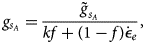
where $\dot {\epsilon }_e$ is the observed effective strain rate, f is a floatation mask, where f = 1 denotes floating ice and f = 0 denotes grounded ice. The constant k is approximately the same order of magnitude as the strain rates (k = 10−2 s−1 in this study), and $\tilde {g}_{a_A}$
 and $\tilde {g}_{s_A}$
 are constants chosen to ensure that the terms ${\tilde {g}_{a_A}}/{k}$
 and ${\tilde {g}_{s_A}}/{k}$
 are approximately the regularization coefficients that would be used without strain rates, to ensure that the regularization balance is maintained across the grounding line.
Supplement Figure S1 presents our approach, similar to an L-curve approach, to determining these coefficients in which we vary the regularization coefficients used and evaluate the resulting misfit to determine how well the inversion performed. We show that some combinations of regularization coefficients fail to decrease the misfit to a reasonable range, while others do significantly better. The coefficients used in this study are presented in Table S2 of the Supplement and are of the same magnitudes as the regularization coefficients applied to the classical regularization case. This ensures that any changes we see in the inferences between the two cases are due to the inclusion of the strain rates and the resulting spatial variability of the coefficients, rather than being because of differences in the magnitude of the regularization coefficients we use.
The formulation presented in Eqns (13) and (14) faces difficulty in areas of very small strain rates, since the regularization coefficients will then get arbitrarily large. In Antarctic Ice Streams, this is unlikely to be a significant problem due to the rapid rates of deformation and therefore this form of regularization can be used effectively in ice streams. However, this method cannot be used reliably outside of ice streams, in areas of low rates of deformation.
The third column of Figure 1 shows the result of the inversion that includes strain rates in the regularization. The misfit decreases to a small value in comparison to the average velocity. The inversion continues to capture the spatial variability of the slipperiness field when including the strain rates. The errors in some of the peaks of the slipperiness distribution are smaller with the strain rates than without, suggesting that the strain rates may have enabled a more accurate resolution of magnitude. This inversion also captures the spatial variability of the flow-rate parameter, with relatively high values in the margins. There is decreased mixing in the center line, suggesting that the inclusion of strain rates in the regularization partitions the domain into regions where ice is deforming relatively rapidly and the model is more sensitive to values of the flow-rate parameter, and regions where there is little deformation in the ice and thus low sensitivity to the values of the flow-rate parameter. However, there is a systematic overestimation of the flow-rate parameter near the grounding line by about a factor of 2. This is likely due to increasing strain rates towards the grounding line (Supplement Fig. S2), and may be mitigated by a more spatially variable regularization coefficient. We expect that for such a small overestimate (less than a factor of 2), the effect on the results for Antarctic Ice Streams is likely to be minimal. We reserve further exploration of this overestimate for future work.
This synthetic test considers the case of high- frequency spatial variability in basal slipperiness, which is often the case for some Antarctic Ice Streams. However, many ice streams have lower frequency spatial variability in basal slipperiness. We conducted tests on a slipperiness field with smaller (in the magnitude of the peak) Gaussian spikes and a long-wavelength background field that increases the slipperiness closer to the grounding line. The regularization coefficients are presented in Table S3 of the Supplement, the regularization coefficients in Figure S4 of the Supplement, and the results in Figure S3 of the Supplement. The inversion resolves spatial distributions in both parameters, with less dramatic mixing even in the case without strain rates. The minimization of mixing may be because the two parameters vary in different directions (basal slipperiness varies along with the flow and the flow-rate parameter varies across flow) and thus there is an inherent spatial disjointness in the inversion. Because of the lower magnitude of the Gaussian spikes, the inversion is slightly better at resolving variations in magnitude. We consider here only the case of ice streams and reserve for future work a thorough investigation of more complex spatial variations in basal slipperiness, the flow-rate parameter, and the geometry of the glacier that may be expected in areas other than ice streams.
While in these synthetic tests, we approximate ‘slippery patches’ in the basal slipperiness field, in which the magnitude of the Gaussian bumps in the slipperiness field is larger than the mean- field, many studies have found evidence of ‘sticky patches’ in Antarctic Ice Streams, a localized decrease in basal slipperiness. Figure S5 in the Supplement presents the results of a similar test with ‘sticky patches’, in which the Gaussian bumps are less than the mean-field. Here, we see similar results to the test presented here. The inversion captures all of the spatial variations in basal slipperiness, except one misplaced sticky spot. The inversion captured the sharp increase in the flow-rate parameter in the shear margins and the flow-rate parameter field shows little mixing between the estimates, likely due to the inclusion of strain rates in the regularization.
The above tests are conducted without added errors in observed velocities. Surface velocity datasets, widely available, are extensive in coverage and have errors much smaller than the magnitude of surface velocity on Antarctica (Gardner and others, Reference Gardner2018). However, any uncertainties in the surface velocity datasets would impact the results of the inversion. Results from a synthetic inversion using measurement errors suggest that, while errors in surface velocity would add noise to the inferred distribution, the large-scale structure and magnitude of basal slipperiness and the flow-rate parameter would still be quite accurate.
Data of ice thickness and basal topography, on the other hand, have more significant errors (Fretwell and others, Reference Fretwell2013). Uncertainties in ice thickness in particular are likely to affect results of inversions, especially estimates of the flow-rate parameters (Eqns (6) and (7)). This is a limitation of inverse methods as applied to any glaciological problem, and more work needs to be done to determine the effect that current uncertainties in data related to glacier geometry may have on the results of glaciological inversions. We leave for future work an in-depth examination of the effect of noise in ice thickness and basal topography on estimates of the flow-rate parameter and the basal slipperiness coefficient.
Results of synthetic tests presented here suggest that inverse methods can provide accurate estimates of basal slipperiness and the flow-rate parameter in Antarctic Ice Streams. Our synthetic tests assume an ice stream geometry, in which the width is much smaller than the length of the glacier, and no-slip lateral margins that are consistent with Antarctic Ice Streams. Furthermore, our synthetic tests assume certain structures of the flow-rate parameter and basal slipperiness that are found in observations and previous inversions on Antarctic Ice Streams (MacAyeal, Reference MacAyeal1992; Echelmeyer and others, Reference Echelmeyer, Harrison, Larsen and Mitchell1994; MacAyeal and others, Reference MacAyeal, Bindschadler and Scambos1995; Joughin and others, Reference Joughin, MacAyeal and Tulaczyk2004; Arthern and others, Reference Arthern, Hindmarsh and Williams2015; Gardner and others, Reference Gardner2018). The inclusion of strain rates into regularization is a strategy that takes advantage of our knowledge of ice stream dynamics and is thus not necessarily applicable to other types of glaciers and ice flow. Thus, this is not necessarily a universal approach.
In particular, the need for further studies is important where basal slipperiness and ice rheology might be expected to vary with the same spatial pattern. Figures S6 and S7 of the Supplement show the results of a synthetic test in which the true flow-rate parameter distribution is constant and the true basal slipperiness distribution varies along-flow and varies in localized Gaussian spikes as shown in Figure 1, respectively. Since the flow-rate parameter does not increase at the margins, and the changes in strain rate are not due to variations in the flow-rate parameter, this approach presented here does not mitigate mixing as it does in Figure 1. Further testing would be required to ascertain whether these inverse methods apply to other outlet glaciers with different glacier geometries or to other glaciers that may have different structures of basal slipperiness and the flow-rate parameter. However, for the case of Antarctic Ice Streams, we have a good physical justification for the flow-rate parameter being higher in the margins thus the results shown here enable us to make use of inverse methods to improve our understanding of Antarctic Ice Streams.
Bindschadler and MacAyeal Ice Streams
The ice streams on the Siple Coast, West Antarctica, are of particular interest to the study of ice flow in outlet glaciers because these ice streams slip over weak sediment, introducing the possibility that shear stress in the lateral margins plays a significant role in controlling ice flow (MacAyeal, Reference MacAyeal1992; Echelmeyer and others, Reference Echelmeyer, Harrison, Larsen and Mitchell1994; Joughin and others, Reference Joughin, MacAyeal and Tulaczyk2004). As a result, the ice streams on the Siple Coast are appealing targets for applying the methods developed above and offer natural laboratories for studying shear-margin processes. Here, we infer basal slipperiness and ice rheology over two Siple Coast ice streams, Bindschadler and MacAyeal Ice Streams, using inverse methods that include strain rates in the regularization term.
Model and data
Previous studies have applied inverse methods similar to those described above with ‘classical’ regularization (e.g., Joughin and others, Reference Joughin, MacAyeal and Tulaczyk2004), but increased quantity and quality of satellite data in the last few years enable more accurate inversions. Inversions require data of bed topography, surface elevation, and surface velocity. Ice-penetrating radar data are used to derive bed topography, and in Figure 2c, we show the radar coverage for Bedmap2, overlaid with contours of observed surface velocity (magenta line; Gardner and others, Reference Gardner2018). While extensive in the ice streams, particularly in Bindschadler Ice Stream, radar coverage contains gaps evident in the shear margins. Fretwell and others (Reference Fretwell2013) estimated the uncertainty in the bed elevation to be ~60 m in the Siple Coast. We use surface topography data from the Reference Elevation Model of Antarctica (REMA) (Fig. 2b), which computes surface elevation from satellite imagery (Howat and others, Reference Howat, Porter, Smith, Noh and Morin2019). Here, we use the filled elevation data with a spatial resolution of 200 m. The elevation error is estimated to be ~0.15–1.2 m in the Siple Coast (Howat and others, Reference Howat, Porter, Smith, Noh and Morin2019). Ice thickness (Fig. 2f) is computed from the difference of REMA elevation data (Fig. 2b) and basal topography from Bedmap2 (Fig. 2d) (Fretwell and others, Reference Fretwell2013; Howat and others, Reference Howat, Porter, Smith, Noh and Morin2019).
Model domain and data used in the inversion: (a) the red outline in the inset shows the location of the model domain, with grounded ice in light gray and floating ice in dark gray. Optical imagery of Bindschadler and MacAyeal Ice Streams from MODIS Mosaic of Antarctica (Scambos and others, Reference Scambos, Haran, Fahnestock, Painter and Bohlander2007), (b) surface elevation from the REMA, (c) radar coverage used to produce bed topography, (d) bed topography from Bedmap2, (e) surface velocity derived from a combination of Landsat 7 and Landsat 8 satellite imagery (Gardner and others, Reference Gardner2018), (f) ice thickness computed as the difference of surface elevation from REMA and bed topography from Bedmap2, (g) effective strain rates ($\dot {\epsilon }_e = \sqrt {\lpar {1}/{2}\rpar \dot {\epsilon }_{ij} \dot {\epsilon }_{ij}}$ ) computed from surface velocity observations (panel e), (f) driving stress computed from the product of ice thickness (panel f), ice density, and surface slope.
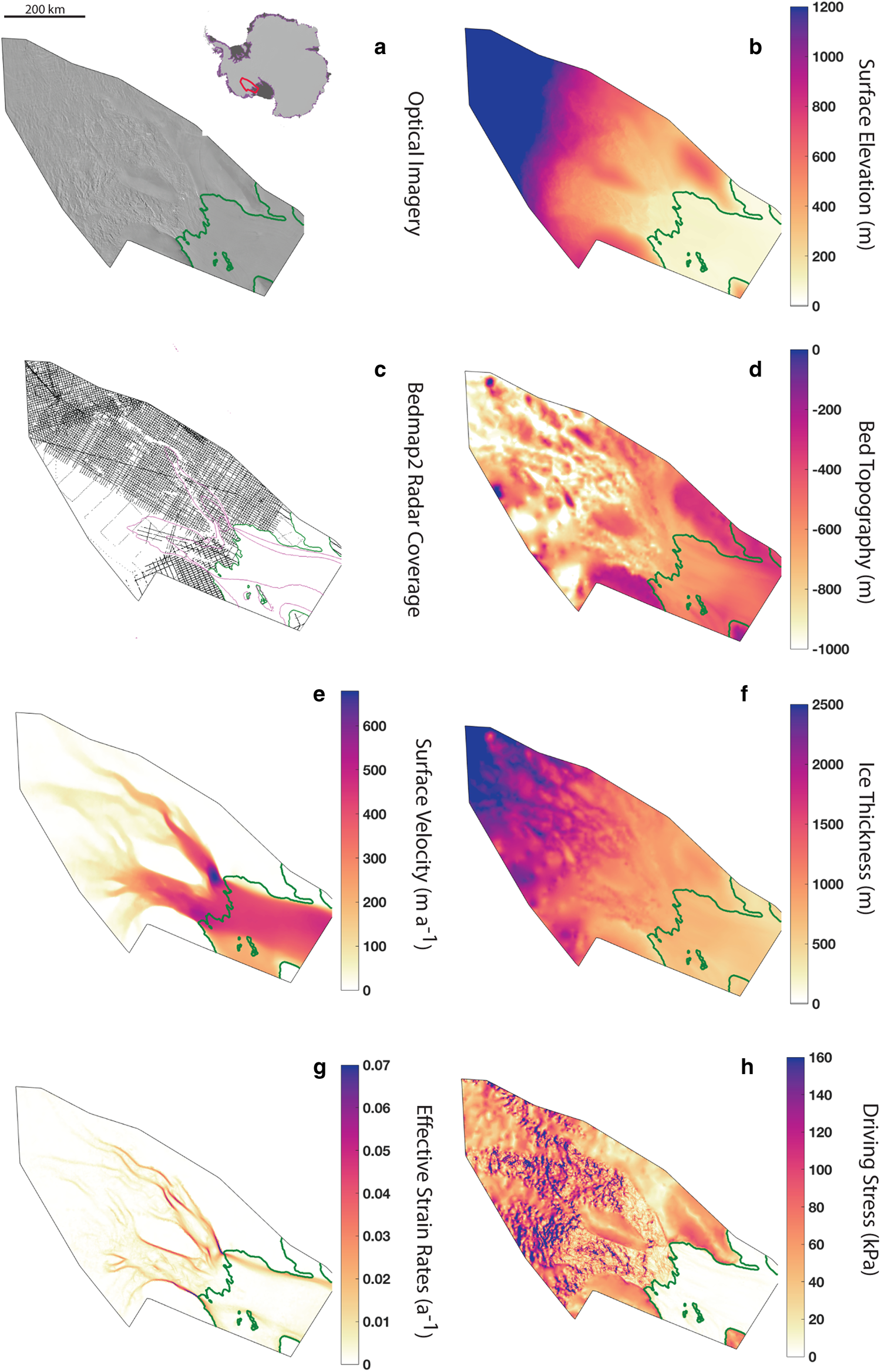
Surface velocities (Fig. 2e) are found from Landsat 7 and 8 satellite data from 2013 to 2015 and the velocity uncertainties are taken on average to be 30 m a−1 (Gardner and others, Reference Gardner2018), which is the error we set for the inversion. The fast flowing regions are moving at ~ 600 m a−1, and the branches of the ice stream at around 300 m a−1. The observed grounding lines are defined from Bedmap2 (Fretwell and others, Reference Fretwell2013) and outlined in green in all panels. The effective strain rates (Fig. 2g), computed from the gradient of the observed velocity fields, demonstrate the high levels of deformation found in the margins. The mean driving stress (Fig. 2h) is ~ 20 kPa and shows a generally decreasing trend with increasing surface velocity, indicating that slip along the bed is the dominant flow regime (Supplement Fig. S8).
The model domain, boundary conditions, and mesh represent the grounded ice streams and proximal regions of the ice shelf. The mesh of the model, constructed in Úa, is refined using observed effective strain rates. We use a relatively fine mesh of ~24000 nodes and 48000 elements, resulting in a spatially varying spatial resolution of a few kilometers (between 1 and 10 km, with finer resolution in areas of high-strain rates). The grounding line in Úa is defined by the floatation condition and closely matches the grounding line of Bedmap2 for the given geometry, though it does not capture some pinning points on the ice shelf because these features are not represented in the Bedmap2 bathymetry (Fig. 2d). The boundary conditions are prescribed to be no-slip at the edges of the grounded model domain, which is chosen to lie only in areas with slow-flowing ice, and are set to be the observed velocities where the model domain is over floating ice.
The inversion is run with spatially constant priors. Based on the tabulated values of the temperature-dependent flow-rate parameter (MacAyeal and others, Reference MacAyeal, Bindschadler and Scambos1995; Cuffey and Paterson, Reference Cuffey and Paterson2010) and an understanding of ice temperature in rapidly-deforming regions of ice sheets (Meyer and Minchew, Reference Meyer and Minchew2018), we estimate the ice temperature to be −10°C, leading to a spatially constant value of the flow-rate parameter A 0 = 1.15 × 10⁻⁸ a−1 kPa−3 (Cuffey and Paterson, Reference Cuffey and Paterson2010). We prescribe the prior of the slipperiness coefficient to be spatially constant at c 0 = 0.01 m a−1 kPa−3. We use strain rates in the regularization coefficients as in Eqn (14) and show the regularization coefficients in the Supplement Figure S9.
Results
Inferred values of basal slipperiness and the flow-rate parameter yield a relatively good fit to the observed velocity fields (Fig. 3). The surface velocity misfit (defined as the difference between the observed and modeled surface velocity scaled by u err = 30 m a−1) is within ( −2, 2) (Fig. 3a), with no obvious structure to the misfit. Areas of high misfit are generally colocated with gaps in radar coverage (Fig. 2c) and errors in the modeled grounding line (Fig. 3a), so we do not expect further reductions in the misfit.
Model misfit and inferred values of basal slipperiness (c) and the flow-rate parameter (A). (a) The velocity misfit (the difference of observed and modeled surface velocity divided by data errors) is within the data errors (|misfit| <1) over most of the model domain. High misfit regions line up with areas of poor radar coverage (Fig. 2c) while areas of good radar coverage have |misfit| <1. (b) The estimate of basal slipperiness shows increased slipperiness towards the grounding line of Bindschadler Ice Stream and the highest values of slipperiness nearest the grounding line. (c) The estimate of the flow-rate parameter has high values that line up with the margins of the ice streams and a less pronounced southern shear margin on the ice shelf of Bindschadler Ice Stream. Dashed lines in panels b and c represent 100 m a−1 velocity contour.
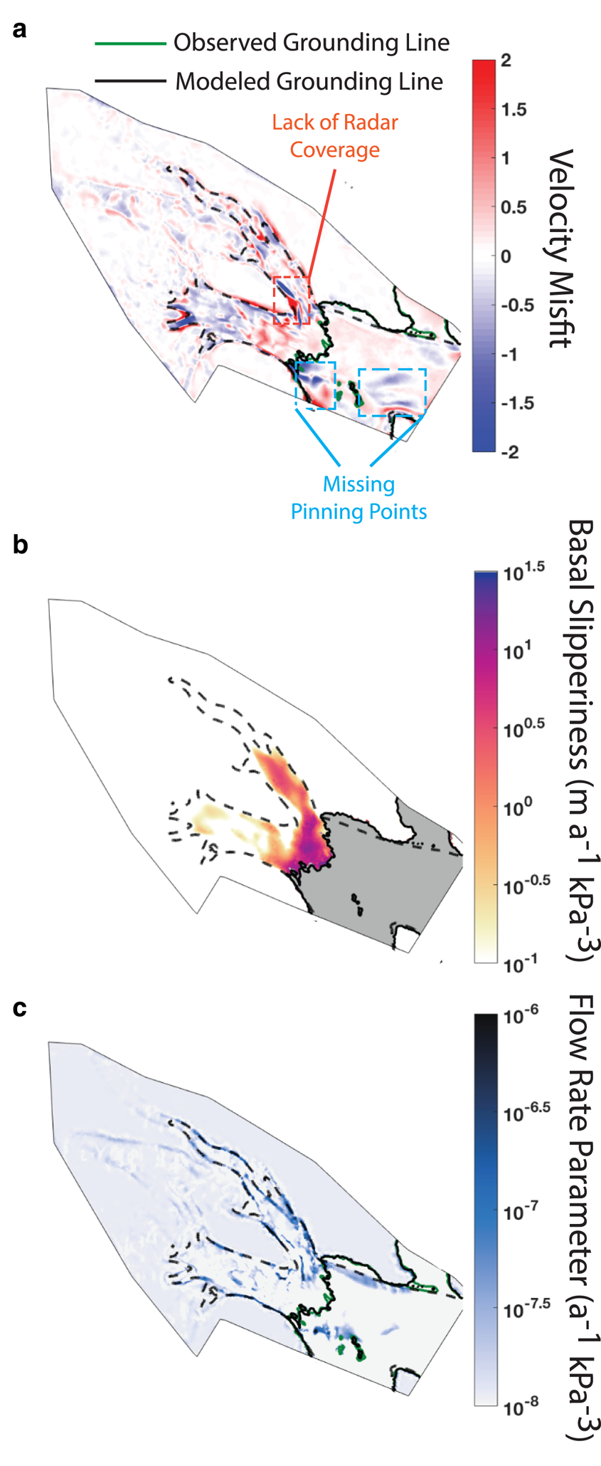
Higher values of the slipperiness distribution extend along the two ice streams. Areas of particularly high slipperiness occur in fast-flowing regions. The maximum slipperiness is ~ 25 m a−1 kPa−3 near where Bindschadler and MacAyeal Ice Streams merge. Elevated slipperiness extends 120 km upstream in Bindschadler Ice Stream with little spatial variability and tapers off as the ice stream narrows. Lower values of slipperiness along MacAyeal correspond to sticky spots that have been identified by previous inversions (MacAyeal, Reference MacAyeal1993; MacAyeal and others, Reference MacAyeal, Bindschadler and Scambos1995; Joughin and others, Reference Joughin, MacAyeal and Tulaczyk2004) and are colocated in areas with steep surface slopes (Figs 2a, h).
The flow-rate parameter is higher in the lateral shear margins of both ice streams. Rapid rates of deformation manifest in the margins, which can result in high rates of work. Some of this work is irreversibly converted to heat, which warms cold ice and melts temperate ice (e.g. Schoof, Reference Schoof2004, Reference Schoof2012; Perol and Rice, Reference Perol and Rice2015; Schoof and Hewitt, Reference Schoof and Hewitt2016), while the rest is accounted for by recrystallization processes. The flow-rate parameter increases with temperature, liquid water content, and development of fabric, and thus is higher in the shear margins.
Some spatial variability in the inferred flow-rate parameter may be a product of the inversion. In particular, variability on the ice shelf may be due to errors in the modeled grounding line (Fig. 3a). There is a sudden decrease in the flow-rate parameter where there is a lack of radar coverage (Fig. 2c) and an increase in velocity misfit (Fig. 3a). Given the results of synthetic tests, values of the flow-rate parameter near the grounding line may be overestimated and the values upstream may be underestimated. However, with the inclusion of strain rates, the variability in the center line of Bindschadler and MacAyeal is likely due to the ice deformation rather than mixing or other errors. The results are qualitatively similar to the results of an inversion without the strain rates in the regularization (Fig. S11 of the Supplement), but it is quantitatively somewhat different and we expect it to be more accurate based on the results of the synthetic tests. Furthermore, this suggests that including the strain rates in the regularization does not create the spatial structure in the flow-rate parameter, but rather it improves the accuracy of the estimated structure.
Discussion
Basal processes
We compute basal drag (Fig. 4a) from basal slipperiness through the sliding law (Eqn (9)) and find basal drag in the slower-flowing regions upstream to be between 120 and 160 kPa, while basal drag in fast-flowing regions is of order 1–10 kPa. These results are consistent with previous studies: MacAyeal and others (Reference MacAyeal, Bindschadler and Scambos1995) found basal stress values to vary from 0.01 to 100 kPa along MacAyeal Ice Stream, while Joughin and others (Reference Joughin, MacAyeal and Tulaczyk2004) expanded this study to both Bindschadler and MacAyeal Ice Streams, finding the maximum of basal stress values to be ~120 kPa. Outside of the ice streams, drag is generally higher (~100 kPa), with the exception of the ridges and southern shear margin of Bindschadler Ice Stream, where surface slopes are shallow. There is increased basal drag south of the southern Bindschadler shear margin immediately upstream of the grounding line, which may direct the flow inward as the ice stream flows onto the ice shelf, thereby playing an important role in controlling the width of the ice stream.
Estimates of (a) basal drag, which shows low drag over most of the fast-flowing regions and prominent sticky spots along MacAyeal. (b) The ratio of basal stress to driving stress indicates that basal drag does not balance driving stress over much of the ice streams. High-frequency variations in the ice streams arise from disparities in spatial resolution. (c) Log of effective pressure, which shows, among other things, the sticky spots in MacAyeal Ice Stream. (d) Log of pore water pressure, which is roughly equivalent to the overburden pressure, suggesting water-saturated till beneath Bindschadler and MacAyeal Ice Streams. Dashed lines represent the 100 m a−1 velocity contour. The ice shelf is shown in gray where basal drag is negligible and not inferred in the inversion.
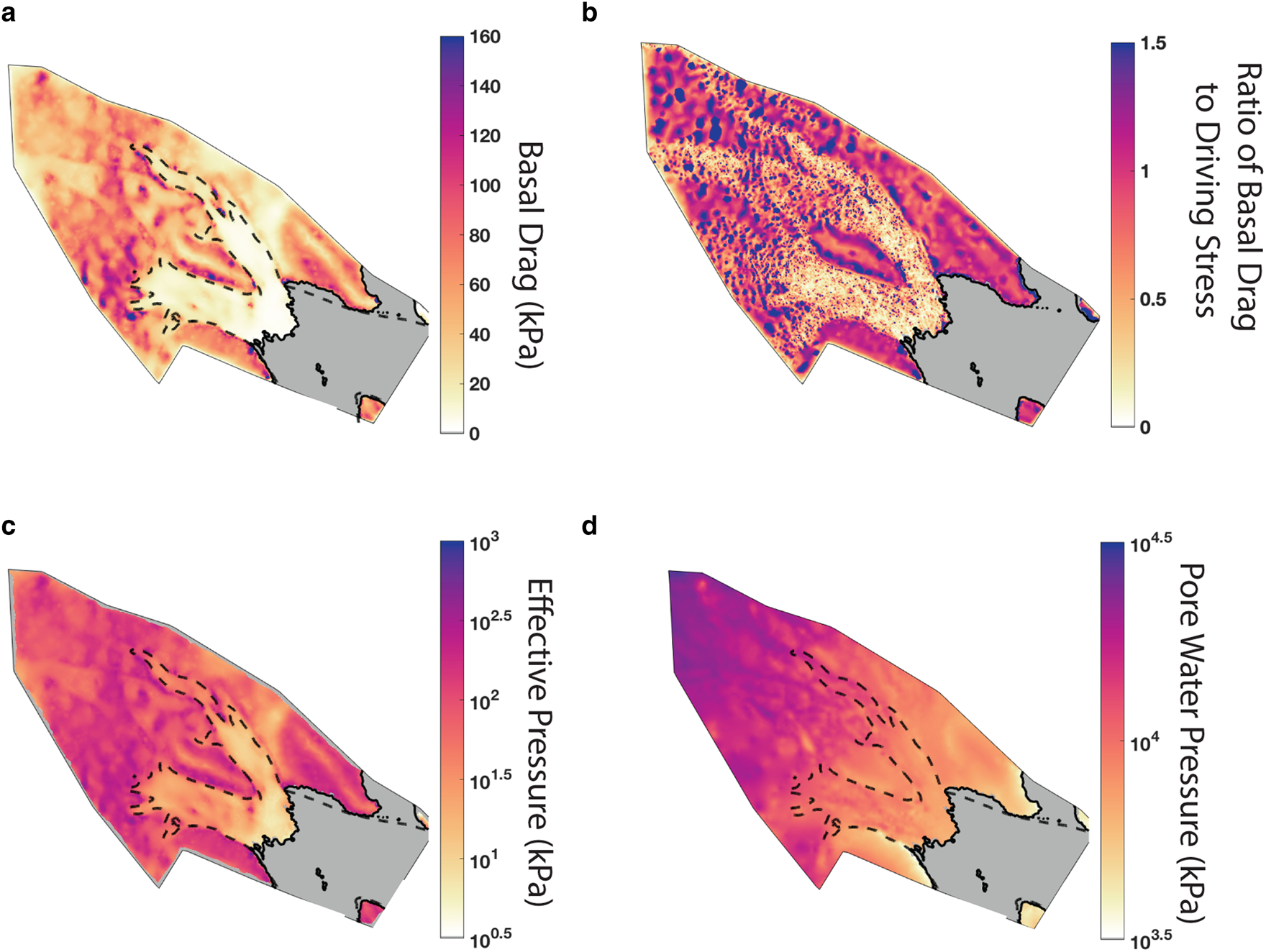
The spatial variability of basal drag is higher in MacAyeal Ice Stream than in Bindschadler Ice Stream. In particular, sticky spots are evident along MacAyeal Ice Stream as localized points of high drag and coincide with steep surface topography (Figs 2a, h). These sticky spots have been identified in past work as well (MacAyeal, Reference MacAyeal1993; MacAyeal and others, Reference MacAyeal, Bindschadler and Scambos1995; Joughin and others, Reference Joughin, MacAyeal and Tulaczyk2004). These sticky spots are colocated with changes in bed topography (Fig. 2d), and previous studies suggest that they are a result of topographic changes, rather than changes in the subglacial hydrologic systems (MacAyeal, Reference MacAyeal1992; MacAyeal and others, Reference MacAyeal, Bindschadler and Scambos1995).
To the best of our knowledge, the ice streams on the Siple Coast are underlain by deformable till (Kamb, Reference Kamb1991; MacAyeal and others, Reference MacAyeal, Bindschadler and Scambos1995). Past studies suggest that this till is water-saturated, and thus basal drag does not balance the driving stress (MacAyeal and others, Reference MacAyeal, Bindschadler and Scambos1995; Joughin and others, Reference Joughin, MacAyeal and Tulaczyk2004). Our results support this supposition: the ratio of basal drag to driving stress is less than one over most of the ice streams (Fig. 4b). The fact that basal shear stress is insufficient to balance the driving stress indicates lateral shear stress at the margins is an important factor in controlling the flow. This is further discussed in the next section.
Laboratory tests indicate that the subglacial till collected from beneath some ice streams in West Antarctica can be well approximated as a perfectly plastic material, meaning that the shear strength of the till is independent of the rate of deformation (Kamb, Reference Kamb1991; Iverson and others, Reference Iverson, Hooyer and Baker1998; Tulaczyk and others, Reference Tulaczyk, Kamb and Engelhardt2000a, Reference Tulaczyk, Kamb and Engelhardt2000b, Zoet and Iverson, Reference Zoet and Iverson2018). This has been further supported by model results: Iverson and Iverson (Reference Iverson and Iverson2001) found that displacement profiles of till are well reproduced from a plastic bed. The yield stress of a perfectly plastic material $\tau _\ast$ can be described by the Mohr–Coulomb criterion $\tau _\ast = c_0 + \mu N$
 (Kamb, Reference Kamb1991; Tulaczyk and others, Reference Tulaczyk, Kamb and Engelhardt2000a), in which c 0 is the apparent cohesion, μ = tan ϕ is the internal friction coefficient (with ϕ being the internal friction angle), and N = ρgH − p w is the effective pressure, where p w is pore water pressure. From laboratory tests, Tulaczyk and others (Reference Tulaczyk, Kamb and Engelhardt2000b) and Iverson (Reference Iverson2010) found that cohesion is negligible and μ ≈ 1/2. The yield stress then becomes $\tau _\ast = \lpar {1}/{2}\rpar N$
 . We assume that deformation of the bed facilitates fast flow (MacAyeal and others, Reference MacAyeal, Bindschadler and Scambos1995) and thus take the basal drag beneath Bindschadler and MacAyeal Ice Streams to be equal to the yield stress. We then compute the effective pressure (Fig. 4c) and pore water pressure (Fig. 4d) from the inferred basal drag.
The effective pressures are low along the length of the ice streams compared to the overburden pressure (overburden pressure is of order 10 MPa, effective pressure is of order 100 kPa). The pore water pressure is comparable to the overburden pressure, supporting the notion that the bed is water-saturated and helping to explain how comparatively low driving stresses can result in high surface velocity. Engelhardt and Kamb (Reference Engelhardt and Kamb1997) used borehole measurements to determine the effective pressure of the till underneath Whillans ice stream (located to the south of Bindschadler and MacAyeal Ice Streams) and found the effective pressure to range from −30 to 160 kPa, which supports our findings of an effective pressure order of magnitude less than the overburden pressure.
Estimates of effective pressure are only valid where the assumption of a yielding bed is valid. This occurs in the fast-flowing sections of the ice streams (seen by the contours of velocity in Fig. 4). Outside of the ice stream, this assumption does not hold and thus estimates of effective pressure and pore water pressure are not reliable. If the bed is not yielded, effective pressure is likely to be larger than shown here.
Spatial variability in effective pressure (Fig. 4c) may be a result of variations in pore water pressure and ice thickness. Due to low gradients in pore water pressure (Fig. 4d), the southern shear margin appears to be pinned by locally elevated effective pressures that arise from locally elevated overburden pressure, rather than locally reduced pore water pressure. The importance of overburden pressure in elevating the effective pressure is in contrast to the findings of Meyer and others (Reference Meyer, Yehya, Minchew and Rice2018), who proposed that the margin was pinned by a locally reduced pore water pressure facilitated by a subglacial channel fed by meltwater from the shear margin. However, the coarse spatial resolution of our inferences, the gap in radar coverage (Fig. 2c), and the smoothness in the slipperiness distribution imposed by the regularization does not necessarily contradict the findings of Meyer and others (Reference Meyer, Yehya, Minchew and Rice2018).
From the small gradients of the pore water pressure, we infer a relatively low flux of water at the bed. This is consistent with low rates of meltwater production and a saturated bed. However, these results are constrained by the resolution of our estimates and the fact that the regularization imposes smoothness and thus inferences of the gradient of pore water pressure may not capture high-frequency spatial variability.
Shear margin processes
Since the basal stress does not balance the gravitational driving stress (Fig. 4b), lateral shear stresses in the margins are important resistances to the flow. Therefore the flow of the ice stream does a lot of work on the ice in the shear margins. The rate of work done during viscous deformation is $\Phi = \sigma _{ij} \dot {\epsilon }_{ij}$ (Jacobson and Raymond, Reference Jacobson and Raymond1998; Schoof, Reference Schoof2004; Schoof and Hewitt, Reference Schoof and Hewitt2016; Hewitt and Schoof, Reference Hewitt and Schoof2017), where σij is the Cauchy stress tensor (Eqn (1)). Under the assumption of incompressibility and applying the constitutive relation for ice (Eqn (4)):

Rates of deformation are highest in the lateral shear margins, and so the work rate is higher in the shear margins than in the trunk of the ice streams and surrounding ridges (Fig. 5a). Since the work done on the ice goes into recrystallization processes or is dissipated as heat, we expect heating and the evolution of crystalline fabric to be higher in the margins as well, resulting in softer ice in lateral shear margins. The variability in the work rate on the ice shelf also reflects the variability in the inferred flow-rate parameter (Fig. 3c) and the observed effective strain rates (Fig. 2g).
(a) Work rate (computed from the inferred flow-rate parameter), which is high in the margins where there are increased levels of deformation and thus heat generation through viscous dissipation. (b) The ratio of inferred flow-rate parameter to the flow-rate parameter for temperate ice A 0 = A r = 1.67 × 10⁻⁷ a−1 kPa−3, which is >1 in some regions of the lateral shear margins. (c) An estimate of the flow-rate parameter (‘effective A T’) found from the 1D thermomechanical model derived in Meyer and Minchew (Reference Meyer and Minchew2018). (d) The ratio of effective A T to the inferred A found by the inversion.
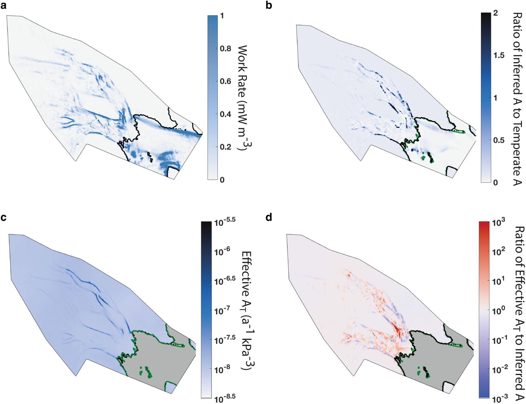
Higher inferred values of the flow-rate parameter in the shear margins suggest localized warming of ice (Jezek and others, Reference Jezek, Alley and Thomas1985; Suckale and others, Reference Suckale, Platt, Perol and Rice2014). Localized warming can occur from internal heating due to the viscous deformation (Jacobson and Raymond, Reference Jacobson and Raymond1998; Schoof, Reference Schoof2004, Reference Schoof2012), which may generate interstitial meltwater, enabling enhanced deformation of the ice (Hewitt and Schoof, Reference Hewitt and Schoof2017; Haseloff and others, Reference Haseloff, Hewitt and Katz2019). Observational evidence supports internal heating in areas of high deformation (Harrison and others, Reference Harrison, Echelmeyer and Larsen1998) and gaps in the radar coverage in the shear margins (Fig. 2c) are consistent with higher radar attenuation expected in warm ice (Schroeder and others, Reference Schroeder, Grima and Blankenship2016). Our findings are also consistent with previous modeling studies. For example, Jacobson and Raymond (Reference Jacobson and Raymond1998), Suckale and others (Reference Suckale, Platt, Perol and Rice2014), and Perol and Rice (Reference Perol and Rice2015) used thermomechanical models to suggest that heat generated may be significant enough to produce temperate ice in shear margins of Antarctic Ice Streams, and Meyer and others (Reference Meyer, Yehya, Minchew and Rice2018) and Meyer and Minchew (Reference Meyer and Minchew2018) show this may be true in Bindschadler Ice Stream.
Internal heating may have implications for ice stream dynamics beyond the softening of ice in the shear margins. Previous studies have proposed the interaction between heating in shear margins and drainage at the bed as a mechanism for control of shear margin location. Perol and Rice (Reference Perol and Rice2015) and Perol and others (Reference Perol, Rice, Platt and Suckale2015) suggested the temperate ice in shear margins may support less lateral stress than the colder ice towards the center of the ice stream, necessitating an increase in basal strength. They attribute this increase in basal strength to the development of a channelized drainage system at the bed, which should result in a decrease of pore water pressure in margins of ice streams. Meyer and others (Reference Meyer, Yehya, Minchew and Rice2018) applied this theory to the southern shear margin of Bindschadler Ice Stream and found evidence for a channelized drainage system near temperate zones and locally decreased pore water pressure. They suggest this may be a control over the width of Bindschadler Ice Stream. The formation of these drainage systems is dependent on significant meltwater production in shear margins.
However, internal heating may not be the sole softening mechanism. The formation of crystallographic preferred orientation (fabric) can also soften the ice. In Figure 5b, we compare the ratio of our inferred flow-rate parameter to the flow-rate parameter value corresponding to temperate ice (A r, given by Cuffey and Paterson, Reference Cuffey and Paterson2010). There are large regions, localized mainly along the shear margins, where the ratio A > A r. Since the temperature of ice cannot exceed the melting temperature throughout the ice column, the regions where the ratio exceeds one are difficult to explain simply by ice temperature. These high values may be explained by the presence of interstitial meltwater, enabling faster flow as described above. This could also be evidence of ice softening due to the evolution of fabric. The existence of a crystallographic preferred orientation, in which the grains of ice are oriented in a similar direction, would suggest that not all of the work done through viscous deformation is dissipated as heat.
We find evidence for potential fabric effects on the flow-rate parameter by comparing the depth-averaged value of the flow-rate parameter given by a thermomechanical model to that inferred in our inversions. We use a model of ice temperature from Meyer and Minchew (Reference Meyer and Minchew2018), which considers the effects of vertical advection and diffusion, to find a depth-averaged flow-rate parameter (‘effective A T’), assuming a solely temperature-dependent flow-rate parameter (Fig. 5c). The ice shelf is not considered here since the thermomechanical model cannot account for spatial variability in the inferred values of the rate factor in areas of the ice shelf that do not show high shear strain rates. The structure of effective A T is similar to the flow-rate parameter estimated by our inversion, providing a check that our inversion results agree with a thermomechanical model.
The effective A T values in the shear margins are on average two orders of magnitude lower than those found by our inversion in the shear margins (Fig. 5d). This could either suggest that inversion is overestimating the flow-rate parameter throughout the ice stream margins or may be evidence that fabric effects play a significant role. The results of synthetic tests (Fig. 1) lead us to believe that we are not overestimating the flow-rate parameter throughout the margins (if any overestimation is occurring, it is likely concentrated near the grounding line). These results agree with Minchew and others (Reference Minchew, Meyer, Robel, Gudmundsson and Simons2018), who found that changes in fabric increase the flow-rate parameter by an order of magnitude, consistent with a single maximum fabric. Fabric development, influenced by recrystallization processes and resulting in anisotropy, are potential mechanisms for ice softening (van der Veen and Whillans, Reference van der Veen and Whillans1994; Duval and Castelnau, Reference Duval and Castelnau1995, Cuffey and others, Reference Cuffey2000a, Reference Cuffey, Thorsteinsson and Waddington2000b) that are often not considered when modeling the development of rheology in shear margins. These results establish an initial hypothesis that anisotropy and dynamic recrystallization are important mechanisms in Antarctic Ice Streams.
There is insufficient evidence to accurately attribute inferred softening to any particular mechanism, but more accurate estimates of the flow-rate parameter presented here are a step forward in being able to understand heating and recrystallization and their influence on ice rheology in shear margins. An examination of the dominant softening mechanisms in shear margins is the desired direction for future research, following work done by Jacobson and Raymond (Reference Jacobson and Raymond1998); Suckale and others (Reference Suckale, Platt, Perol and Rice2014); Haseloff and others (Reference Haseloff, Schoof and Gagliardini2015); Meyer and Minchew (Reference Meyer and Minchew2018); Minchew and others (Reference Minchew, Meyer, Robel, Gudmundsson and Simons2018) on shear margins and work done by Alley, Reference Alley1992; van der Veen and Whillans, Reference van der Veen and Whillans1994; Duval and Castelnau, Reference Duval and Castelnau1995, Cuffey and others, Reference Cuffey2000a, Reference Cuffey, Thorsteinsson and Waddington2000b (among many others) on fabric effects on ice flow. Future work will delve more deeply into the specific mechanisms acting in glacier shear margins.
Summary and conclusion
As more satellite data become available, inverse methods are increasingly critical in accurately modeling ice flow from outlet glaciers. Here, we conduct a systematic study with synthetic data to determine how accurate these methods are for inversions of basal slipperiness and the flow-rate parameter simultaneously in ice streams. By considering spatial variations in basal slipperiness and the flow-rate parameter consistent with those expected in ice streams, we show that these methods can accurately resolve both parameters using surface velocity data and given knowledge of bed topography and surface elevation. We determine that some mixing occurs between the two parameters due to the nonuniqueness of the problem, and further show that including strain rates in the regularization term in the cost function reduces mixing and enables a more accurate decoupling of the flow-rate parameter and slipperiness coefficient. Thus, inverse methods are a useful class of techniques to infer basal slipperiness and the flow-rate parameter in ice streams. This is a critical first step to using the results of these simultaneous inversions to understand and predict ice flow.
We apply these methods to Bindschadler and MacAyeal Ice Streams in the Siple Coast of West Antarctica to find estimates of basal slipperiness and the flow-rate parameter. Estimates of basal slipperiness indicate spatial variability and low basal drag values, which support previous findings that the Siple Coast ice streams sit on weak, deformable, water-saturated till and exhibit sticky spots. Estimates of the flow-rate parameter show high values in the margins of both ice streams that diminish as the ice streams advect over the grounding line. Estimates of the viscous work rate support past findings that the rates of deformation in some portions of the shear margins in Bindschadler and MacAyeal Ice Streams may be sufficient to produce temperate ice and changes in crystallographic fabric and grain size in shear margins. Further research is needed to understand rates of heating through viscous dissipation and dynamic recrystallization, and the relative influence of softening of the ice through heating, interstitial melting, grain rotation and recrystallization, and macroscopic damage.
While successful in synthetic experiments, the methods we present here remain constrained. In particular, these methods are subject to uncertainties in ice thickness and bed topography. Both of these datasets lack complete and uniform coverage in Antarctica and many areas have high uncertainties in the estimates that do exist. Thus, while our approach to inverting for basal drag and ice rheology produces viable results in well-constrained areas such as the Siple Coast, areas with more sparse data coverage may prove challenging. We leave for future work a study of the effect of uncertainties in basal topography and ice thickness in inverse methods. Furthermore, as more accurate remote sensing data comes in and more sophisticated techniques become widely available, these datasets will become more accurate and these inverse methods will become increasingly useful in more geographic locations.
Acknowledgments
M.I.R. was funded through the Callahan Dee Fellowship and the Sven Treitel Fellowship. No new data were produced for this study, and data used in this study are publicly available through their respective publications. The source code for the model Úa is publicly available on Zenodo with DOI 10.5281/zenodo.3706624. The code to run the inversions can also be found there. The code that generates the ice streams and defines the parameters for the inversions for the synthetic tests and Bindschadler and MacAyeal can be found at https://github.com/megr090/Inversion_BasalDragIceRheology.
Supplementary material
To view supplementary material of this article, please visit https://doi.org/10.1017/jog.2020.95


 Open access