


Impact Statement
Quantifying gait patterns can enhance the understanding of disease progression or response to interventions, which is particularly relevant for individuals with multiple sclerosis (MS). In this context, wearable sensors emerge as a cost-effective and unobtrusive tool for patient monitoring. However, the quantitative evaluation of the impact of a disease on gait and mobility using data collected by wearable sensors remains a challenging task. This is primarily due to substantial variability between individuals and temporal fluctuations within a single individual’s data. The work presented here proposes a novel data-driven probabilistic approach which can help reveal which part of the gait cycle is most affected by a disease using a Bayesian machine learning technique, the Hierarchical Variational Sparse Heteroscedastic Gaussian Process.
1. Introduction
Gait is a complex dynamic process that has received increased attention by the scientific community due to its relevance in understanding human health and pathology. Gait impairment, often considered a hallmark of neuromuscular diseases (Polhemus et al., Reference Polhemus, Delgado-Ortiz, Brittain, Chynkiamis, Salis, Gaßner, Gross, Kirk, Rossanigo, Taraldsen, Balta, Breuls, Buttery, Cardenas, Endress, Gugenhan, Keogh, Kluge, Koch, Micó-Amigo, Nerz, Sieber, Williams, Bergquist, de Basea, Buckley, Hansen, Mikolaizak, Schwickert, Scott, Stallforth, van Uem, Vereijken, Cereatti, Demeyer, Hopkinson, Maetzler, Troosters, Vogiatzis, Yarnall, Becker, Garcia-Aymerich, Leocani, Mazzà, Rochester, Sharrack, Frei, Puhan and Mobilise2021; Cicirelli et al., Reference Cicirelli, Impedovo, Dentamaro, Marani, Pirlo and D’Orazio2022), is notably exemplified in multiple sclerosis (MS). This neurodegenerative condition is characterized by the inflammatory-mediated demyelination of axons within the central nervous system (Comber et al., Reference Comber, Galvin and Coote2017). For an enhanced understanding and quantification of the disease, it is necessary to accurately characterize the lower limb distal motion, as it is often affected as a result of alterations in distal muscle involvement (Filli et al., Reference Filli, Sutter, Easthope, Killeen, Meyer, Reuter, Lörincz, Bolliger, Weller, Curt, Straumann, Linnebank and Zörner2018; Pau et al., Reference Pau, Leban, Deidda, Putzolu, Porta, Coghe and Cocco2021; Polhemus et al., Reference Polhemus, Delgado-Ortiz, Brittain, Chynkiamis, Salis, Gaßner, Gross, Kirk, Rossanigo, Taraldsen, Balta, Breuls, Buttery, Cardenas, Endress, Gugenhan, Keogh, Kluge, Koch, Micó-Amigo, Nerz, Sieber, Williams, Bergquist, de Basea, Buckley, Hansen, Mikolaizak, Schwickert, Scott, Stallforth, van Uem, Vereijken, Cereatti, Demeyer, Hopkinson, Maetzler, Troosters, Vogiatzis, Yarnall, Becker, Garcia-Aymerich, Leocani, Mazzà, Rochester, Sharrack, Frei, Puhan and Mobilise2021). As such, the shank angular velocity emerges as a potential signal of interest within this context. While the existing literature predominantly employs the shank angular velocity for gait cycle detection, emphasizing its effectiveness in identifying key gait event landmarks (Pacini Panebianco et al., Reference Panebianco, Bisi, Stagni and Fantozzi2018), the authors assert that the full potential of this signal remains largely unexplored. Additionally, advancements in wearable sensor technology, particularly inertial measurement units (IMUs), have led to their increased application in clinical gait analysis (Angelini et al., Reference Angelini, Hodgkinson, Smith, Dodd, Sharrack, Mazzà and Paling2020). Owing to their flexibility, IMUs present practical solutions for quantifying lower limb distal motion, providing a direct measure of the shank angular velocity, and further motivating the clinical utility of this signal. In light of these considerations, the current work proposes a new approach which seeks to model the full kinematic signal of the shank angular velocity using a data-driven approach. As a first step before exploring longitudinal gait changes, this model is used to reveal regions of the gait cycle that are most affected by the disease or exhibit the greatest variation between contralateral limbs or individuals.
A gait cycle—which consists of the stance phase (accounting for approximately the first $ 60\% $
of the gait cycle) and the swing phase (accounting for the remainder of the gait cycle)—ends and begins with the heel strike event (Rueterbories et al., Reference Rueterbories, Spaich, Larsen and Andersen2010). During the stance phase, the limb bearing the body weight transitions from heel strike to toe-off. During the mid-stance, the body is transitioned forward, and the opposite, contralateral limb is in the swing phase. This part of the gait cycle is characterized by a small base of support and a relatively high center of gravity, making the walker least stable. The swing phase, encompassing initial swing, the mid-swing, and terminal swing, propels the limb forward in preparation for the subsequent heel strike. Figure 1 shows typical examples of shank angular velocity signals during a gait cycle, collected using wearable sensors, for two distinct groups of individuals: healthy controls (HCs) and people with MS (PwMS). Relative to the HC group, the MS group exhibits increased gait pattern variability, particularly discernible from mid-stance to mid-swing. For clarity, the term “variability” is commonly employed in gait analysis to signify stride-to-stride fluctuations during walking, often serving as an indicator of gait impairment (Moon et al., Reference Moon, Sung, An, Hernandez and Sosnoff2016). However, within the scope of this study, “variability” refers to the dispersion of shank angular velocity around its mean characteristic pattern throughout the normalized gait cycle. Although a direct comparison with the relevant literature presents challenges, as the majority of the studies focus on joint kinematics, rather than segment kinematics (as in the case of the present study), similar trends have been previously documented. Crenshaw et al. (Reference Crenshaw, Royer, Richards and Hudson2006) reported a significantly higher knee and ankle joint angle variability for PwMS. Kelleher et al. (Reference Kelleher, Spence, Solomonidis and Apatsidis2010) proposed that individuals with MS experience insufficient propulsion from the ankle plantar flexor muscles and lack fine motor control during the swing phase, perhaps as a result of favoring the more proximal muscle groups. A reduced range of ankle flexion was also confirmed by Nogueira et al. (Reference Teixeira, Sabino, Filho, RMP and Thuler2013), even for PwMS in the prodromal phase of the disease. Similar trends were also reported by Severini et al. (Reference Severini, Manca, Ferraresi, Caniatti, Cosma, Baldasso, Straudi, Morelli and Basaglia2017). More recently, Salehi et al. (Reference Salehi, Mofateh, Mehravar, Negahban, Tajali and Monjezi2020) investigated the deviation phase as a measure of coordination variability and reported significant differences between HC and MS gait during the stance and swing phases. The increased variability observed in the MS group may also be attributed to inefficient gait compensations prompted by factors such as muscle weakness, spasticity, fatigue, or balance impairments (Nogueira et al., Reference Teixeira, Sabino, Filho, RMP and Thuler2013; Socie et al., Reference Socie, Sandroff, Pula, Hsiao-Wecksler, Motl and Sosnoff2013; Gil-Castillo et al., Reference Gil-Castillo, Alnajjar, Koutsou, Torricelli and Moreno2020).
$ 60\% $
of the gait cycle) and the swing phase (accounting for the remainder of the gait cycle)—ends and begins with the heel strike event (Rueterbories et al., Reference Rueterbories, Spaich, Larsen and Andersen2010). During the stance phase, the limb bearing the body weight transitions from heel strike to toe-off. During the mid-stance, the body is transitioned forward, and the opposite, contralateral limb is in the swing phase. This part of the gait cycle is characterized by a small base of support and a relatively high center of gravity, making the walker least stable. The swing phase, encompassing initial swing, the mid-swing, and terminal swing, propels the limb forward in preparation for the subsequent heel strike. Figure 1 shows typical examples of shank angular velocity signals during a gait cycle, collected using wearable sensors, for two distinct groups of individuals: healthy controls (HCs) and people with MS (PwMS). Relative to the HC group, the MS group exhibits increased gait pattern variability, particularly discernible from mid-stance to mid-swing. For clarity, the term “variability” is commonly employed in gait analysis to signify stride-to-stride fluctuations during walking, often serving as an indicator of gait impairment (Moon et al., Reference Moon, Sung, An, Hernandez and Sosnoff2016). However, within the scope of this study, “variability” refers to the dispersion of shank angular velocity around its mean characteristic pattern throughout the normalized gait cycle. Although a direct comparison with the relevant literature presents challenges, as the majority of the studies focus on joint kinematics, rather than segment kinematics (as in the case of the present study), similar trends have been previously documented. Crenshaw et al. (Reference Crenshaw, Royer, Richards and Hudson2006) reported a significantly higher knee and ankle joint angle variability for PwMS. Kelleher et al. (Reference Kelleher, Spence, Solomonidis and Apatsidis2010) proposed that individuals with MS experience insufficient propulsion from the ankle plantar flexor muscles and lack fine motor control during the swing phase, perhaps as a result of favoring the more proximal muscle groups. A reduced range of ankle flexion was also confirmed by Nogueira et al. (Reference Teixeira, Sabino, Filho, RMP and Thuler2013), even for PwMS in the prodromal phase of the disease. Similar trends were also reported by Severini et al. (Reference Severini, Manca, Ferraresi, Caniatti, Cosma, Baldasso, Straudi, Morelli and Basaglia2017). More recently, Salehi et al. (Reference Salehi, Mofateh, Mehravar, Negahban, Tajali and Monjezi2020) investigated the deviation phase as a measure of coordination variability and reported significant differences between HC and MS gait during the stance and swing phases. The increased variability observed in the MS group may also be attributed to inefficient gait compensations prompted by factors such as muscle weakness, spasticity, fatigue, or balance impairments (Nogueira et al., Reference Teixeira, Sabino, Filho, RMP and Thuler2013; Socie et al., Reference Socie, Sandroff, Pula, Hsiao-Wecksler, Motl and Sosnoff2013; Gil-Castillo et al., Reference Gil-Castillo, Alnajjar, Koutsou, Torricelli and Moreno2020).
Comparison of shank angular velocity data between healthy controls (HC) and individuals with multiple sclerosis (MS). The figure presents an aggregate of data points collected using inertial measurement units from both left and right limbs, encompassing 7899 gait cycles from 28 healthy controls and 7105 gait cycles from 28 individuals affected by multiple sclerosis.

From a modeling perspective, it can be seen that the gait signals are exhibiting a number of interesting features. First, the relationship between the input domain and the shank angular velocity is not linear. Second, the variance in the data is not constant across the input space. This phenomenon is known as a heteroscedastic noise process, where the variance in the data is dependent on the input (Or the noise variance changes across the input domain and can be modeled as a function of the input.). In contrast, the process when the variance is independent of the input is referred to as a homoscedastic noise process. Third, inspecting Figure 1, which displays the datapoints from repeated gait cycles collected during straight-line walking for multiple individuals belonging to both groups, it is clear that there is a shared underlying pattern. This observation not only underscores the commonalities in gait dynamics between HC and PwMS but also prompts an exploration of the hierarchical structure inherent in the process of data acquisition during gait assessments. Starting with the collection of data from both lower (contralateral) limbs, this initial stage of organization extends to an individual level, encapsulating the unique characteristics of each participant’s gait. This aspect holds particular relevance in the context of neurological conditions (Rodríguez-Martín et al., Reference Rodríguez-Martín, Samà, Pérez-López, Català, Moreno Arostegui, Cabestany, Bayés, Alcaine, Mestre, Prats, Cruz Crespo, Counihan, Browne, Quinlan, ÓLaighin, Sweeney, Lewy, Azuri, Vainstein, Annicchiarico, Costa and Rodríguez-Molinero2017; Ingelse et al., Reference Ingelse, Branco, Gjoreski, Guerreiro, Bouca-Machado and Ferreira2022). Subsequently, the aggregation of individual-level datasets contribute to the formation of distinct groups (HC and MS in the case of this work). Finally, group categorizations, in turn, become nested within the broader population of individuals, representing a diverse spectrum of human gait patterns. This approach can offer a comprehensive understanding that considers individual variations, group dynamics, and shared trends across the entire population. However, to the best of the authors’ knowledge, the methods currently adopted in the gait-analysis community do not necessarily capture the hierarchical structure of the acquired data. Where many methods presented in the literature will look at a set of summary features—usually computed from data which has been averaged across multiple gait cycles—this article proposes to model the functional form of shank angular velocity across the gait cycle. This approach can be interpreted as a nonparametric representation of the gait. The equivalent feature space is expected to be much richer than a low-dimensional one and has the advantage of not requiring “expert” selection of those features.
In view of the gait characteristics of PwMS and considering the distinctive features observed in the dataset depicted in Figure 1, this study pioneers a novel methodology for constructing a robust probabilistic model specifically tailored to the shank angular velocity. The probabilistic approach proposed in this work may potentially provide valuable insights in the field of gait analysis, especially in the challenging context of assessing and quantifying the degree of gait impairment and its changes over time. In the context of neurological disorders, such as MS, which is marked by intrinsically unpredictable disease progression (Gelfand, Reference Gelfand and Goodin2014; Creagh et al., Reference Creagh, Dondelinger, Lipsmeier, Lindemann and De2022), the proposed probabilistic framework becomes particularly relevant. A probabilistic framework will provide distributions over the expected gait patterns along with a measure of confidence, allowing informed decision-making in data-driven assessments of pathological gait. This is the opposite of a deterministic approach, where uncertainty is not accounted for, and therefore implies perfect models. A deterministic approach can lead to shortcomings in planning for unforeseen variations or complexities in the individual’s gait. Furthermore, the hierarchical extension can advance the analysis capabilities, allowing for a granular analysis of the gait patterns. Here, idiosyncrasies of an individual’s gait patterns can be immediately captured, together with the corresponding confidence bounds. Moreover, group-level differences can be revealed, as well as isolated. It is therefore clear that a hierarchical probabilistic modeling approach offers tangible benefits for the gait analysis community.
This article aims to provide a methodology for accurately modeling the shank angular velocity through an extension of the hierarchical Gaussian processes (GPs) model proposed by Hensman et al. (Reference Hensman, Lawrence and Rattray2013), which effectively manages heteroscedasticity and facilitates sparse inference. The authors hypothesize that such a model would be able to showcase similar trends consistent with the existing literature on lower limb joint kinematics. Importantly, the model is anticipated to achieve this alignment in a manner that reflects the inherent organization of the dataset. The contribution of this paper can be summarized into three key modeling ideas. First, the hierarchical structure inherent in the data is leveraged to capture the temporally structured covariance between contralateral limbs, individual subjects, and groups. This hierarchy accommodates the shared underlying population patterns across both groups, while also accommodating the characteristic group patterns present in all individuals in each group. Additionally, it considers the extension of distinctive individual patterns to contralateral limbs, in order to deal with the potential presence of lower limb asymmetry characterizing the MS-affected group (Pau et al., Reference Pau, Leban, Deidda, Putzolu, Porta, Coghe and Cocco2021). Second, given the substantial amount of data collected during clinical assessments, this work addresses scalability challenges through variational sparse approximations (Titsias, Reference Titsias2009). This ensures the efficiency of the GP in handling large datasets. Third, recognizing the nonconstant variability of the shank angular velocity across the gait cycle, heteroscedasticity is introduced into the GP framework by modeling the variance as an input-dependent function (Lázaro-Gredilla and Titsias, Reference Lázaro-Gredilla and Titsias2011). This approach leads to a sensitive and informative method for characterizing the shank angular velocity patterns.
The article is organized as follows. First, the relevant literature is presented in Section 1.1. Then, the key concepts necessary for the formulation of the hierarchical GP model are presented in Section 2. Following this, the relevant extensions for handling heteroscedasticity and sparse inference are detailed in Sections 2.1, 2.2, and 2.3. Section 3 introduces an example dataset, which will then be utilized to showcase the potential utility of this newly proposed modeling approach in the context of gait analysis. The applications of the methodology on the chosen case study are presented and discussed in detail in Sections 3.2, 3.3, and 3.4. Finally, the article concludes in Section 4.
1.1. Related work
Within the gait analysis community, various approaches have been used for characterizing the gait patterns, broadly falling into three different categories: conceptual gait models, model-based optimization techniques, and statistical methods. Conceptual gait models consist of a finite set of features extracted from the gait signals and are typically initiated with the accurate identification of gait events within the gait cycle. For example, conceptual gait models have been derived for characterizing the gait patterns of people with Parkinson’s disease (Arcolin et al., Reference Arcolin, Corna, Giardini, Giordano, Nardone and Godi2019), as well as community-dwelling older adults (Verghese et al., Reference Verghese, Holtzer, Lipton and Wang2009; Lord et al., Reference Lord, Galna, Verghese, Coleman, Burn and Rochester2013), people with dementia (Verghese et al., Reference Verghese, Wang, Lipton, Holtzer and Xue2007), or MS (Angelini et al., Reference Angelini, Buckley, Bonci, Radford, Sharrack, Paling, Nair and Mazza2021). Specific to the MS population, Shema-Shiratzky et al. (Reference Shema-Shiratzky, Gazit, Sun, Regev, Karni, Sosnoff, Herman, Mirelman and Hausdorff2019) investigated the deterioration of specific aspects of the gait during a typical 6-minute walking test (6MWT), revealing that key metrics—including cadence, stride time variability, stride regularity, step regularity and gait complexity—significantly deteriorated during the test, relative to HCs. Later, Angelini et al. (Reference Angelini, Hodgkinson, Smith, Dodd, Sharrack, Mazzà and Paling2020) studied gait alterations for patients with moderate and severe MS. The study also incorporated supplementary gait metrics, such as intensity, jerk, regularity, and symmetry, which provide additional insights into overall gait quality and efficiency (Pasciuto et al., Reference Pasciuto, Bergamini, Iosa, Vannozzi and Cappozzo2017). In a subsequent study, Angelini et al. (Reference Angelini, Buckley, Bonci, Radford, Sharrack, Paling, Nair and Mazza2021) proposed the previously mentioned MS-specific conceptual gait model, which comprises metrics categorized into five domains (rhythm/variability, pace, asymmetry, and forward and lateral dynamic balance). This model successfully identified gait abnormalities across different MS disability groups. Nevertheless, a notable challenge in these studies lies in assessing the model’s capacity to generalize across unseen datasets. Moreover, by solely focusing on a limited set of features, the authors argue that a vast amount of costly clinical data—potentially encoding important information about the health condition of specific individuals—is discarded.
Model-based optimization techniques have also been used to gain a better understanding of human walking patterns. These approaches leverage idealized mathematical models and cost functions in order to determine an optimized trajectory of the moving body part (Anderson and Pandy, Reference Anderson and Pandy2001; Neptune et al., Reference Neptune, Clark and Kautz2009; Xiang et al., Reference Xiang, Arora and Abdel-Malek2010; Rasouli and Reed, Reference Rasouli and Reed2021). The optimization problem is formulated as a minimization task over various human performance measures, such as dynamic effort, mechanical energy, metabolic energy, jerk, and stability, while adhering to physical constraints (Xiang et al., Reference Xiang, Arora and Abdel-Malek2010). Yet, although informed modeling strategies are utilized, optimization-based techniques can be an oversimplification of the actual gait dynamics, and some are not representative for pathological populations (Rasouli and Reed, Reference Rasouli and Reed2021). However, the biggest limitation of these approaches is that most optimization techniques output a deterministic pattern, which does not account for the uncertainty associated to the target process (Yun et al., Reference Yun, Kim, Shin, Lee, Deshpande and Kim2014), even though it is well known that human gait involves randomness, which cannot be fully captured (Hausdorff et al., Reference Hausdorff, Peng, Ladin, Wei and Goldberger1995).
Statistical methods offer a viable alternative for predicting gait patterns without the need for pre-defining biomechanical models. By inherently accommodating variations and uncertainties inherent in human walking, these methods present a promising approach. In light of the diverse range of available gait analysis acquisition systems (including motion capture devices, force plates, and inertial measurement units), a multitude of machine-learning techniques such as neural networks (Bishop, Reference Bishop2006), support vector machines (SVMs) (Cortes and Vapnik, Reference Cortes and Vapnik1995; Smola and Schölkopf, Reference Smola and Schölkopf2004), or Gaussian process regression (GPR) (Rasmussen and Williams, Reference Rasmussen and Williams2006) have established themselves as prominent data-driven tools for effectively handling extensive gait data processing and inference. For example, Horst et al. (Reference Horst, Kramer, Schäfer, Eekhoff, Hegen, Nigg and Schöllhorn2016) used SVMs to monitor daily kinematic changes in individual gait patterns. Later, Horst et al. (Reference Horst, Lapuschkin, Samek, Müller and Schöllhorn2019) used both SVMs and neural networks to investigate specific gait features in the gait patterns that can accurately identify specific individuals. Gadaleta et al. (Reference Gadaleta, Merelli and Rossi2016) used a convolutional neural network (CNN) to extract gait features from a single wearable sensor placed on the shank. Later, these features were fed to an SVM classifier for human gait-based person recognition. In a later work, Gadaleta and Rossi (Reference Gadaleta and Rossi2018) used the same approach to form an outlier detection problem for human gait identification. More recently, Fang et al. (Reference Fang, Zhou, Sun, Shan, Wang, Xiang and Zhang2020) developed a gait recognition and prediction model based on a temporal CNN for improving the interactions between exoskeletons used for rehabilitation purposes and their users. Nevertheless, these approaches do not inherently offer uncertainty estimates for predictions and, as such, a distinction should be made between deterministic and probabilistic approaches.
Within this context, GPs have emerged as a powerful probabilistic tool for gait pattern prediction. GPs are nonparametric models that can capture complex patterns and dependencies, without assuming any specific functional form. Moreover, GPR allows comparisons of the gait cycles across the full function space rather than simply on a discrete feature level. Wang et al. (Reference Wang, Fleet and Hertzmann2008) proposed a dynamical GP model for human motion, which was later used by Chun et al. (Reference Chun, Kim, Hong and Park2015) and Hong et al. (Reference Hong, Chun, Kim and Park2019) in order to generate reference trajectories for robotic gait rehabilitation systems. Yun et al. (Reference Yun, Kim, Shin, Lee, Deshpande and Kim2014) also used GPR for mapping body parameters to gait kinematics. Glackin et al. (Reference Glackin, Salge, Greaves, Polani, Slavnić, Ristić-Durrant, Leu and Matjačić2014) attempted to model the lower limb joint kinematics of individual subjects and showed that GPs can learn a mapping between patient’s gait and therapist-assisted gait. However, limited conclusions can be drawn from this study, as a result of the limited number of subjects included. Wu et al. (Reference Wu, Liu, Liu, Chen and Guo2018) introduced GP regression for learning the relationship between body parameters and gait features at different walking speeds, as part of a developmental pipeline designed for individualized lower limb exoskeleton robots, while Chen et al., Reference Chen, Guo, Li, Yan and Jiang2023 used deep GPs for online gait prediction during human–exoskeleton interaction. In a different context, Benemerito et al. (Reference Benemerito, Montefiori, Marzo and Mazzà2022) introduced GPs as a regression tool for efficient sensitivity analysis aimed at reducing the complexity of musculoskeletal modeling, in response to the computational challenges offered by traditional Monte Carlo methods. It can be seen that there have been numerous approaches toward modeling gait patterns and that investigation into this problem is an active field of research. While most of the studies have been directed toward robotics applications utilizing modeling of healthy patterns, GPR adoption for modeling pathological gait patterns remains limited. Additionally, to the best of the author’s knowledge, no studies have specifically attempted the probabilistic modeling of shank angular velocity. Moreover, the challenges associated with the scalability of GPs are seldom addressed (Chen et al., Reference Chen, Guo, Li, Yan and Jiang2023), and the integration of heteroscedastic approaches remains largely unexplored for this specific application. Furthermore, it is also significant to highlight that hierarchical extensions that mimic the organization of the data have not been ventured within the realm of gait analysis, as far as the authors are aware.
To address these challenges, motivated by the characteristics of the example dataset presented in Section 1, this paper provides a novel methodology that forms an accurate hierarchical model for the shank angular velocity kinematics. Concurrently, the varying uncertainty is automatically quantified across the duration of the gait cycle in a manner that is efficient for large datasets and statistically rigorous. The approach proposed in this article integrates the methodologies of Liu et al. (Reference Liu, Ong and Cai2018), which enables sparse inference along with handling of heteroscedastic noise, with a novel application of hierarchical modeling, as originally proposed by Hensman et al. (Reference Hensman, Lawrence and Rattray2013).
2. Gaussian process regression
Gaussian process (GP) models represent a versatile nonparametric Bayesian machine learning approach for resolving regression problems, enabling the characterization of a distribution over functions (Rasmussen and Williams, Reference Rasmussen and Williams2006). Specifically, a GP is an infinite set of random variables that exhibit a joint Gaussian distribution for any finite subset. GPs have gained significant popularity across a diverse range of applications owing to their ability to automatically quantify uncertainty in predictions, minimal requirement for a priori input, and modeling capabilities even in the presence of high noise levels in the measured data. The GP is developed to model data as the output of some function $ f\left(\boldsymbol{x}\right) $
, operating on a
$ f\left(\boldsymbol{x}\right) $
, operating on a $ D $
-dimensional input
$ D $
-dimensional input $ \boldsymbol{x} $
, as described by Equation 1.
$ \boldsymbol{x} $
, as described by Equation 1.
 $$ y=f\left(\boldsymbol{x}\right)+\varepsilon, \hskip0.1em \varepsilon \sim \mathcal{N}\left(0,{\sigma}_n^2\right) $$
Here, it is assumed that the measured values $ \boldsymbol{y} $
differ from the latent function values
$ \boldsymbol{y} $
differ from the latent function values $ f\left(\boldsymbol{x}\right) $
by some additive noise
$ f\left(\boldsymbol{x}\right) $
by some additive noise $ \varepsilon $
with zero mean and a predetermined variance
$ \varepsilon $
with zero mean and a predetermined variance $ {\sigma}_n^2 $
, also known as the “nugget parameter.” Equation 2 formally defines a GP, where
$ {\sigma}_n^2 $
, also known as the “nugget parameter.” Equation 2 formally defines a GP, where $ \boldsymbol{x} $
and
$ \boldsymbol{x} $
and $ {\boldsymbol{x}}^{\prime } $
are a pair of inputs to the function of interest. For clarification, the notation adopted in this study involves representing vectors using bold typography, while matrices are identified by uppercase letters.
$ {\boldsymbol{x}}^{\prime } $
are a pair of inputs to the function of interest. For clarification, the notation adopted in this study involves representing vectors using bold typography, while matrices are identified by uppercase letters.
 $$ f\left(\boldsymbol{x}\right)\sim \mathcal{GP}\left(m\left(\boldsymbol{x}\right),k\left(\boldsymbol{x},{\boldsymbol{x}}^{\prime}\right)\right) $$
It follows that a GP is completely specified by its mean function $ m\left(\boldsymbol{x}\right) $
and the covariance function
$ m\left(\boldsymbol{x}\right) $
and the covariance function $ k\left(\boldsymbol{x},{\boldsymbol{x}}^{\prime}\right) $
. Here, the covariance function encodes the similarity between any pair of inputs. A popular choice for the covariance function is the
$ k\left(\boldsymbol{x},{\boldsymbol{x}}^{\prime}\right) $
. Here, the covariance function encodes the similarity between any pair of inputs. A popular choice for the covariance function is the $ 3/2 $
Matérn kernel, which is described in Equation 3. Although other kernel functions exist, such as the squared exponential kernel, the Matérn kernel was selected, as it was found to better model the abrupt changes in the slope of the gait traces, as a result of its finitely differentiable property.
$ 3/2 $
Matérn kernel, which is described in Equation 3. Although other kernel functions exist, such as the squared exponential kernel, the Matérn kernel was selected, as it was found to better model the abrupt changes in the slope of the gait traces, as a result of its finitely differentiable property.
 $$ k\left(\boldsymbol{x},{\boldsymbol{x}}^{\prime}\right)={\sigma}_f^2\left(1+\frac{\sqrt{3}{\left(\boldsymbol{x}-{\boldsymbol{x}}^{\prime}\right)}^2}{l}\right)\exp \left(\frac{-\sqrt{3}{\left(\boldsymbol{x}-{\boldsymbol{x}}^{\prime}\right)}^2}{l}\right) $$
Note that this kernel function is defined by a set of two hyperparameters: the variance $ {\sigma}_f $
, controlling the vertical scaling (amplitude) of the kernel and the length-scale
$ {\sigma}_f $
, controlling the vertical scaling (amplitude) of the kernel and the length-scale $ l $
, which controls the smoothness of the functions. Next, the prediction task is achieved by assessing the joint Gaussian distribution of the observed target values and the function values at the test locations.
$ l $
, which controls the smoothness of the functions. Next, the prediction task is achieved by assessing the joint Gaussian distribution of the observed target values and the function values at the test locations.
Finally, in order to learn the hyperparameters, a Type-II maximum likelihood (ML-II) approach is used by maximizing the marginal likelihood of the model. However, for convenience and numerical stability, the optimization is performed as a minimization task over the negative log marginal likelihood. For the specific mathematical details regarding GP implementation, the reader is referred to Rasmussen and Williams (Reference Rasmussen and Williams2006) and to Appendix A, where the key equations are presented.
2.1. Sparse GPs for large datasets scalability
Either learning the hyperparameters of the GP or making predictions involves taking the inverse of the covariance matrix with noise, $ {\left({K}_{xx}+{\sigma}_n^2\unicode{x1D540}\right)}^{-1} $
, which is an operation scaling as
$ {\left({K}_{xx}+{\sigma}_n^2\unicode{x1D540}\right)}^{-1} $
, which is an operation scaling as $ \mathcal{O}\left({N}^3\right) $
in computational complexity. Hence, in practice, it is not feasible to perform full GP regression tasks on datasets involving more than roughly 10,000 datapoints (Rogers et al., Reference Rogers, Gardner, Dervilis, Worden, Maguire, Papatheou and Cross2020). This is also one of the limitations preventing the use of full GP regression on gait data, as the number of datapoints collected during a visit often exceeds 10,000 points per subject. To address this limitation, a number of approximation methods have already been proposed in the literature (Quiñonero-Candela and Rasmussen, Reference Quiñonero-Candela and Rasmussen2005; Titsias, Reference Titsias2009; Bui et al., Reference Bui, Yan and Turner2017; Hensman et al., Reference Hensman, Durrande and Solin2018). Broadly speaking, these approaches are divided into two main classes, namely model approximations and posterior approximations. For the sake of brevity, the reader is referred to Quiñonero-Candela and Rasmussen (Reference Quiñonero-Candela and Rasmussen2005), Rasmussen and Williams (Reference Rasmussen and Williams2006), or Bui et al. (Reference Bui, Yan and Turner2017) for more details about these approaches. The posterior approximation approach is widely recognized to generally provide more robust approximations and possess inherent mechanisms to counteract overfitting. Thus, the present study employs a posterior approximation method, specifically the variational free energy (VFE) method proposed by Titsias (Reference Titsias2009). The main advantage of this approximation method is the reduction in time complexity from
$ \mathcal{O}\left({N}^3\right) $
in computational complexity. Hence, in practice, it is not feasible to perform full GP regression tasks on datasets involving more than roughly 10,000 datapoints (Rogers et al., Reference Rogers, Gardner, Dervilis, Worden, Maguire, Papatheou and Cross2020). This is also one of the limitations preventing the use of full GP regression on gait data, as the number of datapoints collected during a visit often exceeds 10,000 points per subject. To address this limitation, a number of approximation methods have already been proposed in the literature (Quiñonero-Candela and Rasmussen, Reference Quiñonero-Candela and Rasmussen2005; Titsias, Reference Titsias2009; Bui et al., Reference Bui, Yan and Turner2017; Hensman et al., Reference Hensman, Durrande and Solin2018). Broadly speaking, these approaches are divided into two main classes, namely model approximations and posterior approximations. For the sake of brevity, the reader is referred to Quiñonero-Candela and Rasmussen (Reference Quiñonero-Candela and Rasmussen2005), Rasmussen and Williams (Reference Rasmussen and Williams2006), or Bui et al. (Reference Bui, Yan and Turner2017) for more details about these approaches. The posterior approximation approach is widely recognized to generally provide more robust approximations and possess inherent mechanisms to counteract overfitting. Thus, the present study employs a posterior approximation method, specifically the variational free energy (VFE) method proposed by Titsias (Reference Titsias2009). The main advantage of this approximation method is the reduction in time complexity from $ \mathcal{O}\left({N}^3\right) $
to
$ \mathcal{O}\left({N}^3\right) $
to $ \mathcal{O}\left({NM}^2\right) $
, where
$ \mathcal{O}\left({NM}^2\right) $
, where $ M $
is the number of auxiliary points introduced, called inducing points, at which the approximation is performed. Clearly, this becomes advantageous when
$ M $
is the number of auxiliary points introduced, called inducing points, at which the approximation is performed. Clearly, this becomes advantageous when $ M\ll N $
. Therefore, with this approximation method, the standard GP can be scaled up to large datasets, such as those containing gait data collected during clinical assessments for multiple patients.
$ M\ll N $
. Therefore, with this approximation method, the standard GP can be scaled up to large datasets, such as those containing gait data collected during clinical assessments for multiple patients.
The variational approximation of the full posterior is handled through the use of a small set of inducing points, $ \left\{Z,\boldsymbol{u}\right\} $
(where Z contains the locations of the inducing points and
$ \left\{Z,\boldsymbol{u}\right\} $
(where Z contains the locations of the inducing points and $ \boldsymbol{u} $
are the values of the latent functions at these points). The model can then be learnt by minimizing the Kullback–Leibler (KL) divergence between the approximate joint posterior and the full joint GP posterior. Nonetheless, this minimization is equivalent to maximizing a variational lower bound (also known as the Evidence Lower Bound or
$ \boldsymbol{u} $
are the values of the latent functions at these points). The model can then be learnt by minimizing the Kullback–Leibler (KL) divergence between the approximate joint posterior and the full joint GP posterior. Nonetheless, this minimization is equivalent to maximizing a variational lower bound (also known as the Evidence Lower Bound or $ ELBO $
) of the true log marginal likelihood, as detailed in Titsias (Reference Titsias2009). For conciseness, the key equations characterizing the variational approximation method used in this paper as a means of scaling GPs to large datasets can be found in Appendix B.
$ ELBO $
) of the true log marginal likelihood, as detailed in Titsias (Reference Titsias2009). For conciseness, the key equations characterizing the variational approximation method used in this paper as a means of scaling GPs to large datasets can be found in Appendix B.
2.2. Sparse heteroscedastic noise models extensions
With reference to the dataset presented in Figure 1, it is evident that the homoscedastic noise assumption of the GP model is not satisfied. This is the assumption that the additive noise on the function $ f\left(\boldsymbol{x}\right) $
has a constant variance across the input space. To address this problem, heteroscedastic GP models (that is those using input-dependent additive noise) have been developed (Lázaro-Gredilla and Titsias, Reference Lázaro-Gredilla and Titsias2011). Focusing on the MS group, it can be seen that gait pattern variability is one of the key aspects of the disease. Hence, enhancing the model’s ability to effectively capture the inherent variability, particularly in the swing phase of the gait cycle, will enable the establishment of more accurate confidence bounds for predictions. In this case, the regression model introduced by Equation 1 would then become
$ f\left(\boldsymbol{x}\right) $
has a constant variance across the input space. To address this problem, heteroscedastic GP models (that is those using input-dependent additive noise) have been developed (Lázaro-Gredilla and Titsias, Reference Lázaro-Gredilla and Titsias2011). Focusing on the MS group, it can be seen that gait pattern variability is one of the key aspects of the disease. Hence, enhancing the model’s ability to effectively capture the inherent variability, particularly in the swing phase of the gait cycle, will enable the establishment of more accurate confidence bounds for predictions. In this case, the regression model introduced by Equation 1 would then become
 $$ y=f\left(\boldsymbol{x}\right)+\unicode{x025B} \left(\boldsymbol{x}\right),\hskip0.1em \unicode{x025B} \left(\boldsymbol{x}\right)\sim \mathcal{N}\left(0,r\left(\boldsymbol{x}\right)\right) $$
This means that the variance of the noise process is now a function of the model inputs. Notably, the heteroscedastic noise model presented above reduces to a homoscedastic one when $ r\left(\boldsymbol{x}\right) $
is a constant. The derivation of the heteroscedastic GP model was first introduced by Lázaro-Gredilla and Titsias (Reference Lázaro-Gredilla and Titsias2011). To define this model, a GP prior is initially placed on the unknown function
$ r\left(\boldsymbol{x}\right) $
is a constant. The derivation of the heteroscedastic GP model was first introduced by Lázaro-Gredilla and Titsias (Reference Lázaro-Gredilla and Titsias2011). To define this model, a GP prior is initially placed on the unknown function $ f\left(\boldsymbol{x}\right) $
, as presented in Equation 5. Here, a zero-mean function has been assumed for practicality reasons, although this assumption is not restrictive, and alternative mean functions can be considered.
$ f\left(\boldsymbol{x}\right) $
, as presented in Equation 5. Here, a zero-mean function has been assumed for practicality reasons, although this assumption is not restrictive, and alternative mean functions can be considered.
 $$ f\left(\boldsymbol{x}\right)\sim \mathcal{GP}\left(0,{k}_f\left(\boldsymbol{x},{\boldsymbol{x}}^{\prime}\right)\right) $$
Then, to ensure positivity of the noise variance, $ r\left(\boldsymbol{x}\right) $
, an exponential transform is applied, as described in Equation 6:
$ r\left(\boldsymbol{x}\right) $
, an exponential transform is applied, as described in Equation 6:
 $$ r\left(\boldsymbol{x}\right)=\exp \left(h\left(\boldsymbol{x}\right)\right),\hskip2em h\left(\boldsymbol{x}\right)\sim \mathcal{GP}\left({\mu}_0,{k}_h\left(\boldsymbol{x},{\boldsymbol{x}}^{\prime}\right)\right) $$
Here, the log noise variance, denoted by $ h\left(\boldsymbol{x}\right) $
is modeled by a GP, whose covariance function is denoted by
$ h\left(\boldsymbol{x}\right) $
is modeled by a GP, whose covariance function is denoted by $ {k}_h\left(\boldsymbol{x},{\boldsymbol{x}}^{\prime}\right) $
. The GP has a constant mean,
$ {k}_h\left(\boldsymbol{x},{\boldsymbol{x}}^{\prime}\right) $
. The GP has a constant mean, $ {\mu}_0 $
, which controls the scale of the noise process. Here
$ {\mu}_0 $
, which controls the scale of the noise process. Here $ {\mu}_0 $
is introduced as a learnable parameter, which models the “average” noise level across the function. This is a departure from standard function modeling where
$ {\mu}_0 $
is introduced as a learnable parameter, which models the “average” noise level across the function. This is a departure from standard function modeling where $ {\mu}_0=0 $
is typically assumed. By learning
$ {\mu}_0=0 $
is typically assumed. By learning $ {\mu}_0 $
, we can account for the inherent noise present in the data, which corresponds to the homoscedastic case. As such, the addition of the secondary GP placed on the log noise variance increases the expressiveness of the GP, albeit simultaneously increasing the complexity of the learning and inference processes. As a result of the inclusion of the heteroscedastic noise model, the log-likelihood becomes untractable and can no longer be computed analytically. Similarly to the sparse GP extension, a variational method is used to approximate the posterior distribution and form a new lower bound. The key equations describing the lower bound and the variational approximation of the first two moments of the predictive distribution are detailed in Appendix C.
$ {\mu}_0 $
, we can account for the inherent noise present in the data, which corresponds to the homoscedastic case. As such, the addition of the secondary GP placed on the log noise variance increases the expressiveness of the GP, albeit simultaneously increasing the complexity of the learning and inference processes. As a result of the inclusion of the heteroscedastic noise model, the log-likelihood becomes untractable and can no longer be computed analytically. Similarly to the sparse GP extension, a variational method is used to approximate the posterior distribution and form a new lower bound. The key equations describing the lower bound and the variational approximation of the first two moments of the predictive distribution are detailed in Appendix C.
The concepts outlined above facilitate the probabilistic estimation of latent underlying functions, along with accurate prediction of variance, at any given input. However, in practice, computing the variational bound of the heteroscedastic GP, along with its gradient, takes roughly twice the time required to compute the evidence and its derivatives in a standard homoscedastic GP (Lázaro-Gredilla and Titsias, Reference Lázaro-Gredilla and Titsias2011). Due to this cost consideration, integrating a variational sparse heteroscedastic method to improve scalability becomes a necessity. To this end, the Variational Sparse Heteroscedastic Gaussian Process (VSHGP) has already been derived in the literature by Liu et al. (Reference Liu, Ong and Cai2018). Inspired by the model presented in Lázaro-Gredilla and Titsias (Reference Lázaro-Gredilla and Titsias2011), Liu et al. (Reference Liu, Ong and Cai2018) have shown that it is possible to derive an analytical $ ELBO $
using
$ ELBO $
using $ M $
inducing points for the mean function GP,
$ M $
inducing points for the mean function GP, $ f\left(\boldsymbol{x}\right) $
, and
$ f\left(\boldsymbol{x}\right) $
, and $ U $
inducing points for approximating the log noise variance GP modeling
$ U $
inducing points for approximating the log noise variance GP modeling $ h\left(\boldsymbol{x}\right) $
. As a result, this approach is scalable to large datasets, given its
$ h\left(\boldsymbol{x}\right) $
. As a result, this approach is scalable to large datasets, given its $ \mathcal{O}\left({NM}^2+{NU}^2\right) $
complexity.
$ \mathcal{O}\left({NM}^2+{NU}^2\right) $
complexity.
Finally, with these methods it is now possible to approximate the first two moments of the predictive distribution, that is the mean and variance, respectively. The nontrivial key equations leading to the derivation of the first two moments can be found in Appendix D. It is also worth noting that, in addition to the methodology presented here, Liu et al. (Reference Liu, Ong and Cai2018) also improved the scalability of the proposed VSHGP model through the addition of stochastic and distributed extensions. However, these extensions are not utilized in this study. For more details regarding these, the reader is instead referred to the original paper. As it will later be demonstrated, the additional information provided by the VSHGP model regarding the uncertainty of the process will prove to be an important capability for modeling kinematic gait patterns, especially in pathological populations.
2.3. Hierarchical expansion
In this study, we reassess the dataset depicted in Figure 1, comprising two distinct subgroups: HCs and PwMS. The final modeling strategy employed herein involves a hierarchical extension of the VSHGP model presented in Section 2.2. This extension entails its integration with the hierarchical model proposed by Hensman et al. (Reference Hensman, Lawrence and Rattray2013). Specific to the current dataset, the key idea of hierarchical models is that there exists a common trend across a pool of data from multiple candidates performing the same walking test, regardless of their group label. The measurements obtained from each participant exhibit individual variation from the shared trend due to biomechanical differences, as well as corruptive noise. Consequently, these distinctive individual gait patterns can be interpreted as individual signatures (Winner et al., Reference Winner, Rosenberg, Jain, Kesar, Ting and Berman2023). For the sake of simplicity, this section will only consider a two-layer hierarchy and will only present the implementation using a standard GP. The integration of the variational sparse heteroscedastic extension in a hierarchical framework will be explained further in this section of the report by considering block-wise relationships within the hierarchical covariance.
Let $ {\boldsymbol{y}}_{gi} $
denote the vector of measurements for the
$ {\boldsymbol{y}}_{gi} $
denote the vector of measurements for the $ i $
th individual in group
$ i $
th individual in group $ g $
. The corresponding time points are stored in vector
$ g $
. The corresponding time points are stored in vector $ {\boldsymbol{x}}_{gi} $
. To combine the data acquired during all the walking tests from all participants in a particular group, a Bayesian hierarchical approach is being used. The underlying trend for the
$ {\boldsymbol{x}}_{gi} $
. To combine the data acquired during all the walking tests from all participants in a particular group, a Bayesian hierarchical approach is being used. The underlying trend for the $ g $
th group,
$ g $
th group, $ {f}_g\left(\boldsymbol{x}\right) $
is presumed to be drawn from a GP with a zero-mean and whose covariance function is denoted by
$ {f}_g\left(\boldsymbol{x}\right) $
is presumed to be drawn from a GP with a zero-mean and whose covariance function is denoted by $ {k}_g\left(\boldsymbol{x},{\boldsymbol{x}}^{\prime}\right) $
. Further down in the hierarchy, the underlying trend describing the gait pattern belonging to a unique participant in that particular group,
$ {k}_g\left(\boldsymbol{x},{\boldsymbol{x}}^{\prime}\right) $
. Further down in the hierarchy, the underlying trend describing the gait pattern belonging to a unique participant in that particular group, $ {f}_{gi}\left(\boldsymbol{x}\right) $
is drawn from the group GP. However, the mean of the individual GP is
$ {f}_{gi}\left(\boldsymbol{x}\right) $
is drawn from the group GP. However, the mean of the individual GP is $ {f}_g\left(\boldsymbol{x}\right) $
, as described in Equation 7.
$ {f}_g\left(\boldsymbol{x}\right) $
, as described in Equation 7.
 $$ {\displaystyle \begin{array}{c}{f}_g\left(\boldsymbol{x}\right)\sim \mathcal{GP}\left(0,{k}_g\left(\boldsymbol{x},{\boldsymbol{x}}^{\prime}\right)\right)\\ {}{f}_{g,i}\left(\boldsymbol{x}\right)\sim \mathcal{GP}\left({f}_g\left(\boldsymbol{x}\right),{k}_i\left(\boldsymbol{x},{\boldsymbol{x}}^{\prime}\right)\right)\\ {}\mathrm{where}\hskip0.24em i=1,2,\dots, n\end{array}} $$
It should be noted that the two covariance functions $ {k}_g $
and
$ {k}_g $
and $ {k}_i $
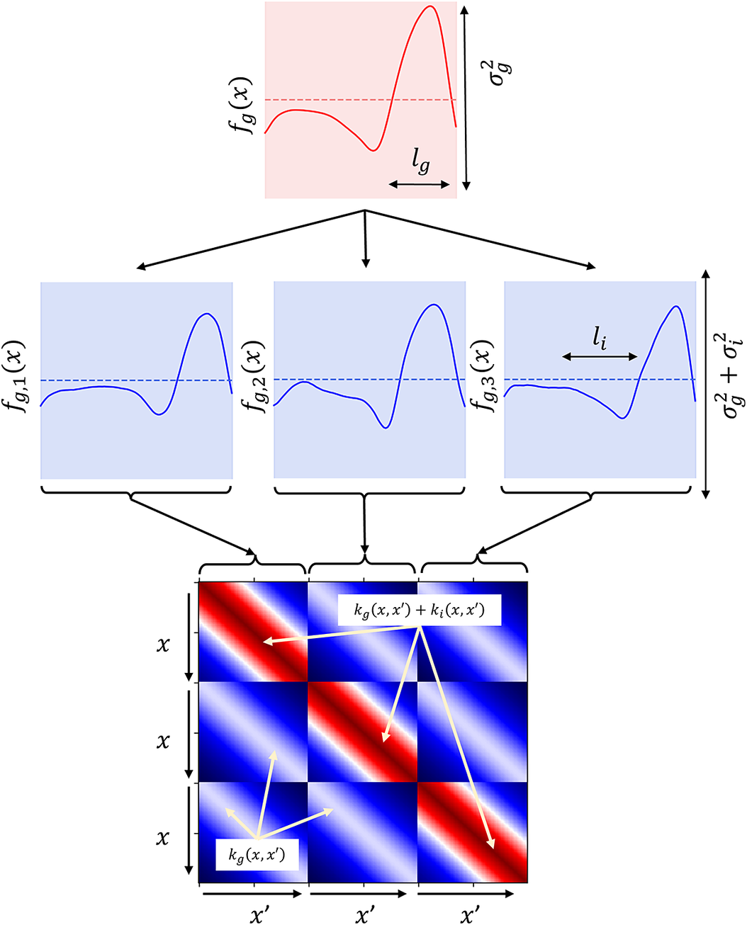
used for the group and individual levels may be different. For clarity, while group kernel hyperparameters remain constant across all individuals, individual kernel hyperparameters are allowed to vary, reflecting specific individual variability. This model is pictorially shown in Figure 2, where the function dependency is highlighted. The prior over the underlying group pattern
$ {k}_i $
used for the group and individual levels may be different. For clarity, while group kernel hyperparameters remain constant across all individuals, individual kernel hyperparameters are allowed to vary, reflecting specific individual variability. This model is pictorially shown in Figure 2, where the function dependency is highlighted. The prior over the underlying group pattern $ {f}_g\left(\boldsymbol{x}\right) $
is shown at the top, as a dotted line. The shaded area represents the variance of the function, which is controlled by
$ {f}_g\left(\boldsymbol{x}\right) $
is shown at the top, as a dotted line. The shaded area represents the variance of the function, which is controlled by $ {\sigma}_g^2 $
. The smoothness of the function is controlled by the length-scale of the group kernel,
$ {\sigma}_g^2 $
. The smoothness of the function is controlled by the length-scale of the group kernel, $ {l}_g $
. A single sample from this prior is then shown as a red solid line,and the length-scale of the covariance function is also highlighted. The individual level is shown in the second row, where samples conditioned on the sample shown in
$ {l}_g $
. A single sample from this prior is then shown as a red solid line,and the length-scale of the covariance function is also highlighted. The individual level is shown in the second row, where samples conditioned on the sample shown in $ {f}_g\left(\boldsymbol{x}\right) $
are displayed, representing three unique individuals. The three samples follow the trend of
$ {f}_g\left(\boldsymbol{x}\right) $
are displayed, representing three unique individuals. The three samples follow the trend of $ {f}_g\left(\boldsymbol{x}\right) $
, but are allowed to independently vary by a small amount (
$ {f}_g\left(\boldsymbol{x}\right) $
, but are allowed to independently vary by a small amount ( $ {\sigma}_i^2 $
) with a short length-scale
$ {\sigma}_i^2 $
) with a short length-scale $ {l}_i $
. Therefore, although the main features of the common trend are preserved, each of the individuals exhibit their own characteristics. Finally, the hierarchical covariance matrix is shown at the bottom of Figure 2, demonstrating the block-wise relationship between individuals.
$ {l}_i $
. Therefore, although the main features of the common trend are preserved, each of the individuals exhibit their own characteristics. Finally, the hierarchical covariance matrix is shown at the bottom of Figure 2, demonstrating the block-wise relationship between individuals.
An illustration of a simple hierarchical GP. Top: solid line—a single sample from the prior over the underlying group function $ {f}_g(x) $
. Dotted line—zero-mean function. Shaded area:
$ {f}_g(x) $
. Dotted line—zero-mean function. Shaded area: $ \pm 1 $
standard deviation of functions,
$ \pm 1 $
standard deviation of functions, $ {\sigma}_g^2 $
. Middle: three samples conditioned on
$ {\sigma}_g^2 $
. Middle: three samples conditioned on $ {f}_g(x) $
and corresponding to three distinct individuals. The individual samples follow the trend of
$ {f}_g(x) $
and corresponding to three distinct individuals. The individual samples follow the trend of $ {f}_g(x) $
, but vary by a small amount,
$ {f}_g(x) $
, but vary by a small amount, $ {\sigma}_i^2 $
. The length-scale of the group and individual functions are denoted by
$ {\sigma}_i^2 $
. The length-scale of the group and individual functions are denoted by $ {l}_g $
and
$ {l}_g $
and $ {l}_i $
, respectively. Bottom: block-wise covariance matrix used to generate samples.
$ {l}_i $
, respectively. Bottom: block-wise covariance matrix used to generate samples.
Let
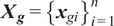
 $ {\boldsymbol{Y}}_{\boldsymbol{g}}={\left\{{\boldsymbol{y}}_{gi}\right\}}_{i=1}^n $
be the collection of noisy observations for
$ {\boldsymbol{Y}}_{\boldsymbol{g}}={\left\{{\boldsymbol{y}}_{gi}\right\}}_{i=1}^n $
be the collection of noisy observations for $ n $
patients in group
$ n $
patients in group $ g $
and
$ g $
and $ {\boldsymbol{X}}_{\boldsymbol{g}}={\left\{{\boldsymbol{x}}_{gi}\right\}}_{i=1}^n $
the corresponding time points. Due to the conjugacy property of Gaussian distributions, the model described above can be mathematically represented as a joint Gaussian distribution, and it is possible to write down the likelihood as
$ {\boldsymbol{X}}_{\boldsymbol{g}}={\left\{{\boldsymbol{x}}_{gi}\right\}}_{i=1}^n $
the corresponding time points. Due to the conjugacy property of Gaussian distributions, the model described above can be mathematically represented as a joint Gaussian distribution, and it is possible to write down the likelihood as
 $$ p\left({\boldsymbol{Y}}_{\boldsymbol{g}}|{\boldsymbol{X}}_{\boldsymbol{g}},\theta \right)\sim \mathcal{N}\left({\hat{\boldsymbol{y}}}_{\boldsymbol{g}}|\mathbf{0},{\Sigma}_g\right) $$
where $ {\hat{\boldsymbol{y}}}_{\boldsymbol{g}}={\left[{\boldsymbol{y}}_{g,1}^T,{\boldsymbol{y}}_{g,2}^T,\dots, {\boldsymbol{y}}_{g,n}^T\right]}^T $
has been used to denote the row-wise concatenation of
$ {\hat{\boldsymbol{y}}}_{\boldsymbol{g}}={\left[{\boldsymbol{y}}_{g,1}^T,{\boldsymbol{y}}_{g,2}^T,\dots, {\boldsymbol{y}}_{g,n}^T\right]}^T $
has been used to denote the row-wise concatenation of $ {\boldsymbol{Y}}_{\boldsymbol{g}} $
.
$ {\boldsymbol{Y}}_{\boldsymbol{g}} $
. $ \theta $
are the hyperparameters of the covariance functions
$ \theta $
are the hyperparameters of the covariance functions $ {k}_g\left(\cdot \right) $
and
$ {k}_g\left(\cdot \right) $
and $ {k}_i\left(\cdot \right) $
. Finally, the block of
$ {k}_i\left(\cdot \right) $
. Finally, the block of $ {\Sigma}_g $
is given by
$ {\Sigma}_g $
is given by
 $$ {\Sigma}_g\left[i,{i}^{\prime}\right]=\left(\begin{array}{ll}{K}_g\left({\boldsymbol{x}}_{gi},{\boldsymbol{x}}_{g{i}^{\prime }}\right)+{K}_i\left({\boldsymbol{x}}_{gi},{\boldsymbol{x}}_{g{i}^{\prime }}\right)+{\sigma}_n^2\unicode{x1D540}& \mathrm{if}\;i={i}^{\prime}\\ {}{K}_g\left({\boldsymbol{x}}_{gi},{\boldsymbol{x}}_{g{i}^{\prime }}\right)& \mathrm{otherwise}.\end{array}\right. $$
In order to make inferences about the functions $ {f}_g\left(\boldsymbol{x}\right) $
and
$ {f}_g\left(\boldsymbol{x}\right) $
and $ {f}_{g,i}\left(\boldsymbol{x}\right) $
, it is necessary to compute the covariances between these functions. The predictive covariance functions are given in Equation 10. Note that these expressions describe the covariance of the latent functions, while the covariance of the observed data
$ {f}_{g,i}\left(\boldsymbol{x}\right) $
, it is necessary to compute the covariances between these functions. The predictive covariance functions are given in Equation 10. Note that these expressions describe the covariance of the latent functions, while the covariance of the observed data $ {y}_{gi} $
additionally includes the heteroscedastic noise variance
$ {y}_{gi} $
additionally includes the heteroscedastic noise variance $ r(x) $
via moment-matching (Lázaro-Gredilla and Titsias, Reference Lázaro-Gredilla and Titsias2011). This means that group predictions can be made simply by using the group kernel,
$ r(x) $
via moment-matching (Lázaro-Gredilla and Titsias, Reference Lázaro-Gredilla and Titsias2011). This means that group predictions can be made simply by using the group kernel, $ {k}_g\left(\cdot \right) $
, whereas an additive kernel,
$ {k}_g\left(\cdot \right) $
, whereas an additive kernel, $ {k}_g\left(\cdot \right)+{k}_i\left(\cdot \right) $
, is required for individual predictions.
$ {k}_g\left(\cdot \right)+{k}_i\left(\cdot \right) $
, is required for individual predictions.
 $$ \mathit{\operatorname{cov}}\left({f}_{gi}(x),\hskip0.3em {f}_g\left({x}^{\prime}\right)\right)={k}_g\left(\boldsymbol{x},{\boldsymbol{x}}^{\prime}\right), $$
 $$ \mathit{\operatorname{cov}}\left({f}_{gi}(x),\hskip0.3em {f}_{g{i}^{\prime }}\left({x}^{\prime}\right)\right)=\left\{\begin{array}{ll}{k}_g\left(\boldsymbol{x},{\boldsymbol{x}}^{\prime}\right)+{k}_i\left(\boldsymbol{x},{\boldsymbol{x}}^{\prime}\right)& \mathrm{if}\;i={i}^{\prime}\\ {}{k}_g\left(\boldsymbol{x},{\boldsymbol{x}}^{\prime}\right)& \mathrm{otherwise}.\end{array}\right. $$
Finally, inference can then be made using the standard methods outlined in the preceding sections, while hyperparameters of the covariance functions can also be optimized in a similar fashion. However, the scalability of the hierarchical model is similar to that of a standard GP, limiting its applicability to large datasets. Hence, to mitigate the computational challenges associated with large datasets, variational approximation methods have been employed to efficiently approximate the posterior distributions, as described in Sections 2.1 and 2.2. The hierarchical formulation employs a shared set of inducing points across all GPs in the hierarchy, in contrast to maintaining distinct sets for each hierarchical level. This formulation serves to both reduce computational complexity and constrain the parameter space, as it requires optimizing a single shared set of inducing point locations rather than multiple disjoint sets across the hierarchy.
3. A case study for characterizing gait variability in MS using hierarchical Gaussian processes
Here, it remains to demonstrate how the above proposed scheme might be applied to gait data collected from both patients and healthy control individuals. The purpose of this case study is to highlight how the framework for modeling of gait (with heteroscedastic noise) provides insights from all levels of the hierarchy, from specific limbs to populations. The examples shown in this section will progress downward from the top of the hierarchy, starting with comparisons between groups of PwMS and HCs, and finishing with considerations of symmetry in individuals’ gait. The dataset used in this work consists of angular velocity data recorded with IMUs from $ 2 $
groups of subjects: namely healthy controls (HCs, with no history of musculoskeletal or neurologic disorders which might affect their balance or mobility) and individuals with MS. Both groups were comprised of
$ 2 $
groups of subjects: namely healthy controls (HCs, with no history of musculoskeletal or neurologic disorders which might affect their balance or mobility) and individuals with MS. Both groups were comprised of $ 28 $
subjects each. The severity of MS was assessed through the Expanded Disablity Status Scale (EDSS) scale (Kurtzke, Reference Kurtzke1983), which is one of the most widely used clinical outcomes (Angelini et al., Reference Angelini, Buckley, Bonci, Radford, Sharrack, Paling, Nair and Mazza2021), consisting of a neurological assessment, as well as observing the walking range and the level of walking assistance needed. The scale is rated from
$ 28 $
subjects each. The severity of MS was assessed through the Expanded Disablity Status Scale (EDSS) scale (Kurtzke, Reference Kurtzke1983), which is one of the most widely used clinical outcomes (Angelini et al., Reference Angelini, Buckley, Bonci, Radford, Sharrack, Paling, Nair and Mazza2021), consisting of a neurological assessment, as well as observing the walking range and the level of walking assistance needed. The scale is rated from $ 0 $
(normal healthy status) to
$ 0 $
(normal healthy status) to $ 10 $
(MS-related death) in 0.5-unit increments. Scores up to
$ 10 $
(MS-related death) in 0.5-unit increments. Scores up to $ 3.5 $
typically indicate no visible gait impairment, while scores between
$ 3.5 $
typically indicate no visible gait impairment, while scores between $ 4.0 $
and
$ 4.0 $
and $ 5.5 $
denote individuals capable of walking limited distances independently. Scores up to
$ 5.5 $
denote individuals capable of walking limited distances independently. Scores up to $ 6.5 $
indicate the necessity of assistive walking devices, while higher scores denote restricted mobility. In this case study, participants with relapse-remitting MS were included only if they had experienced no relapse in the
$ 6.5 $
indicate the necessity of assistive walking devices, while higher scores denote restricted mobility. In this case study, participants with relapse-remitting MS were included only if they had experienced no relapse in the $ 30 $
days preceding the baseline test and had maintained a stable treatment for the past 3 months. No participants using assistive devices were included. Ethics approval was granted by both the NRES Committee Yorkshire & The Humber-Bradford Leeds (Ref: 15/YH/0300) and the North of Scotland Research Ethics Committee (Ref: 17/NS/0020). Written informed consent was obtained from all participants prior to their inclusion in the study.
$ 30 $
days preceding the baseline test and had maintained a stable treatment for the past 3 months. No participants using assistive devices were included. Ethics approval was granted by both the NRES Committee Yorkshire & The Humber-Bradford Leeds (Ref: 15/YH/0300) and the North of Scotland Research Ethics Committee (Ref: 17/NS/0020). Written informed consent was obtained from all participants prior to their inclusion in the study.
Gait data was acquired using two tri-axial IMUs (OPAL, APDM Inc, Portland, OR, USA, sampling frequency, $ 128 $
Hz, gyroscope range
$ 128 $
Hz, gyroscope range $ \pm 2000{}^{\circ}/\mathrm{s} $
), attached to the body through elastic straps, on the anterior aspect of both shanks. The sensing axes of the sensors were approximately aligned with the anatomical planes. Both groups (HC and MS) performed the 6MWT, going back and forth in a straight line across a corridor of either
$ \pm 2000{}^{\circ}/\mathrm{s} $
), attached to the body through elastic straps, on the anterior aspect of both shanks. The sensing axes of the sensors were approximately aligned with the anatomical planes. Both groups (HC and MS) performed the 6MWT, going back and forth in a straight line across a corridor of either $ 10 $
or
$ 10 $
or $ 14 $
m and turning at the ends (Table 1). Participants were instructed to walk at their self-selected pace, with rests permitted only if necessary. All turns and resting breaks were automatically removed, following the procedure detailed in Angelini et al. (Reference Angelini, Buckley, Bonci, Radford, Sharrack, Paling, Nair and Mazza2021). Only straight-line walking bouts were included in the upcoming analysis. Data was segmented into individual strides, according to the gait events locations identified in the shank angular velocity signal (Angelini et al., Reference Angelini, Buckley, Bonci, Radford, Sharrack, Paling, Nair and Mazza2021). To remove sensor misalignment effects, a rotation to a vertical-horizontal coordinate system was applied, as described in Moe-Nilssen (Reference Moe-Nilssen1998). The shank angular velocity signals were filtered with a zero-phase, low-pass, Butterworth filter with a 10 Hz cut-off frequency and normalized using a zero-mean, unit range normalization method. It was decided to remove the transient part at the beginning of the signals (first
$ 14 $
m and turning at the ends (Table 1). Participants were instructed to walk at their self-selected pace, with rests permitted only if necessary. All turns and resting breaks were automatically removed, following the procedure detailed in Angelini et al. (Reference Angelini, Buckley, Bonci, Radford, Sharrack, Paling, Nair and Mazza2021). Only straight-line walking bouts were included in the upcoming analysis. Data was segmented into individual strides, according to the gait events locations identified in the shank angular velocity signal (Angelini et al., Reference Angelini, Buckley, Bonci, Radford, Sharrack, Paling, Nair and Mazza2021). To remove sensor misalignment effects, a rotation to a vertical-horizontal coordinate system was applied, as described in Moe-Nilssen (Reference Moe-Nilssen1998). The shank angular velocity signals were filtered with a zero-phase, low-pass, Butterworth filter with a 10 Hz cut-off frequency and normalized using a zero-mean, unit range normalization method. It was decided to remove the transient part at the beginning of the signals (first $ 8\% $
of the samples), in order to avoid problems caused by misclassification of the gait events (Haji Ghassemi et al., Reference Haji Ghassemi, Hannink, Martindale, Gaßner, Müller, Klucken and Eskofier2018). Finally, for each individual limb, the resultant gait cycles were normalized along the time axis, effectively eliminating the pace component from the signals and facilitating direct comparative analysis.
$ 8\% $
of the samples), in order to avoid problems caused by misclassification of the gait events (Haji Ghassemi et al., Reference Haji Ghassemi, Hannink, Martindale, Gaßner, Müller, Klucken and Eskofier2018). Finally, for each individual limb, the resultant gait cycles were normalized along the time axis, effectively eliminating the pace component from the signals and facilitating direct comparative analysis.
Demographics table

Note. RR, relapse remitting; SP, secondary progressive.
3.1. Case study objectives and model evaluation metrics
Given the anticipated differences among the gait patterns of HCs and PwMS, the aim of this case study is to showcase the intrinsic advantages of the proposed modeling approach. Therefore, having established a mathematical framework for hierarchically modeling the nonlinear gait pattern, together with heteroscedastic noise, the focus can now shift toward predicting the shank angular velocity for the two groups considered in this study. The following results will serve to highlight the benefits of the three main aspects present in the proposed novel modeling methodology. First, it is necessary to establish that the uncertainty found in the gait data is heteroscedastic, warranting this more complex modeling choice and demonstrating the insight that can be learnt from the functional form of the noise variance. Second, it will be shown how the hierarchical nature of the model naturally obeys the structure arising in gait data when aggregating different limbs, individuals, and groups (e.g. MS and HC), and facilitates quantitative comparisons across multiple scales. Finally, considering that angular velocity data was acquired from both limbs, as well as the time normalization procedure used in this study, the third objective of this study is to showcase the utility of the probabilistic models by introducing a novel methodology for lower limb asymmetry quantification. With regards to the third aim of this study, it is important to note that the concept of asymmetry presented here deviates from the traditional concept of gait asymmetry, which is commonly assessed as the absolute difference in temporal metrics between contralateral limbs or as the natural logarithm of the absolute ratio between their mean values (Godfrey et al., Reference Godfrey, Del Din, Barry, Mathers and Rochester2015; Yogev et al., Reference Yogev, Plotnik, Peretz, Giladi and Hausdorff2007). However, the full motivation for alternative asymmetry metrics is postponed until Section 3.4.
A total number of $ \mathrm{50,015} $
gait cycles has been collected, (
$ \mathrm{50,015} $
gait cycles has been collected, ( $ \mathrm{26,330} $
belonging to healthy individuals and
$ \mathrm{26,330} $
belonging to healthy individuals and $ \mathrm{23,685} $
to PwMS). Following pre-processing, the data are separated into two distinct sets: the training set and the held-out test set. The training set consists of
$ \mathrm{23,685} $
to PwMS). Following pre-processing, the data are separated into two distinct sets: the training set and the held-out test set. The training set consists of $ 70\% $
randomly selected samples from the aggregate dataset, that is combined data from all subjects. For clarity, a single sample refers to a single data point. Only this set was used for training and hence the optimization of the hyperparameters. The test set contains the remaining
$ 70\% $
randomly selected samples from the aggregate dataset, that is combined data from all subjects. For clarity, a single sample refers to a single data point. Only this set was used for training and hence the optimization of the hyperparameters. The test set contains the remaining $ 30\% $
of the data, that is these samples remain unseen until predictions are made and are referred to as the held-out test set. The training set contains
$ 30\% $
of the data, that is these samples remain unseen until predictions are made and are referred to as the held-out test set. The training set contains $ \mathrm{1,942,881} $
data points, while the test set contains
$ \mathrm{1,942,881} $
data points, while the test set contains $ \mathrm{832,664} $
points. It can be therefore seen that given the very large datasets, it is not feasible to fit non-variational sparse GPs with any reasonable amount of computational resources. In addition to this, training the GP models on a subset of data (that is downsampled data) may lead to unreliable uncertainty quantification, which fails to capture the full information present in the complete dataset (Quiñonero-Candela and Rasmussen, Reference Quiñonero-Candela and Rasmussen2005). This is particularly important in gait analysis, where both the overall pattern and subtle variations can be clinically relevant. As such, for full transparency, comparisons with standard GP formulations have not been conducted in this study.
$ \mathrm{832,664} $
points. It can be therefore seen that given the very large datasets, it is not feasible to fit non-variational sparse GPs with any reasonable amount of computational resources. In addition to this, training the GP models on a subset of data (that is downsampled data) may lead to unreliable uncertainty quantification, which fails to capture the full information present in the complete dataset (Quiñonero-Candela and Rasmussen, Reference Quiñonero-Candela and Rasmussen2005). This is particularly important in gait analysis, where both the overall pattern and subtle variations can be clinically relevant. As such, for full transparency, comparisons with standard GP formulations have not been conducted in this study.
The hierarchical variational sparse heteroscedastic GP (HVSHGP) model, combining the hierarchical approach, together with sparsity and heteroscedasticity was implemented in Python, using GPflow (de G. Matthews et al., Reference de G. Matthews, van der Wilk, Nickson, Fujii, Boukouvalas, León-Villagrá, Ghahramani and Hensman2017). As an implementation note, instead of constructing the block-wise covariance matrix, the underlying dependencies and interdependencies between different subjects and groups were modeled by incorporating a block-wise relationship into an additive $ ELBO $
, which was then optimized using the NADAM (Nesterov-accelerated Adaptive Moment Estimation) algorithm (Dozat, Reference Dozat2016)—an extension of the Adam optimizer that combines Nesterov momentum with adaptive moment estimation to improve convergence speed and stability. Optimization was performed with a learning rate of 0.0001 for 1000 steps, and default parameters: β
1 = 0.9, β
2 = 0.999. While the derivatives of the lower bound (see Equation 30) with respect to the hyperparameters are provided in the framework proposed by Liu et al. (Reference Liu, Ong and Cai2018), the additive ELBO used in this hierarchical approach was optimized using the automatic differentiation capabilities of TensorFlow (Abadi et al., Reference Abadi, Agarwal, Barham, Brevdo, Chen, Citro, Corrado, Davis, Dean, Devin, Ghemawat, Goodfellow, Harp, Irving, Isard, Jia, Jozefowicz, Kaiser, Kudlur, Levenberg, Mane, Monga, Moore, Murray, Olah, Schuster, Shlens, Steiner, Sutskever, Talwar, Tucker, Vanhoucke, Vasudevan, Viegas, Vinyals, Warden, Wattenberg, Wicke, Yu and Zheng2015). Moreover, it should be noted that optimizing over the size of the inducing point set represents a challenging high-dimensional optimization problem. As such, while the size of the inducing point set is fixed at
$ ELBO $
, which was then optimized using the NADAM (Nesterov-accelerated Adaptive Moment Estimation) algorithm (Dozat, Reference Dozat2016)—an extension of the Adam optimizer that combines Nesterov momentum with adaptive moment estimation to improve convergence speed and stability. Optimization was performed with a learning rate of 0.0001 for 1000 steps, and default parameters: β
1 = 0.9, β
2 = 0.999. While the derivatives of the lower bound (see Equation 30) with respect to the hyperparameters are provided in the framework proposed by Liu et al. (Reference Liu, Ong and Cai2018), the additive ELBO used in this hierarchical approach was optimized using the automatic differentiation capabilities of TensorFlow (Abadi et al., Reference Abadi, Agarwal, Barham, Brevdo, Chen, Citro, Corrado, Davis, Dean, Devin, Ghemawat, Goodfellow, Harp, Irving, Isard, Jia, Jozefowicz, Kaiser, Kudlur, Levenberg, Mane, Monga, Moore, Murray, Olah, Schuster, Shlens, Steiner, Sutskever, Talwar, Tucker, Vanhoucke, Vasudevan, Viegas, Vinyals, Warden, Wattenberg, Wicke, Yu and Zheng2015). Moreover, it should be noted that optimizing over the size of the inducing point set represents a challenging high-dimensional optimization problem. As such, while the size of the inducing point set is fixed at $ 100 $
across all levels of the hierarchy, their locations are treated as optimization variables. This represents a trade-off between computational complexity and model fidelity: fixing the number of inducing points helps manage computational cost, while allowing their locations to be optimized enables the model to better capture the underlying structure of the gait patterns. The optimization of inducing point locations does increase the complexity of the variational optimization problem, but we found this additional flexibility to be beneficial for capturing nuanced gait patterns. For a more thorough discussion about the selection and optimization of the inducing points set, the readers are referred to Quiñonero-Candela and Rasmussen (Reference Quiñonero-Candela and Rasmussen2005) or Bui et al. (Reference Bui, Yan and Turner2017). As a result, a four-layer HVSHGP model was achieved (see Figure 3), and with every layer in the hierarchy, new hyperparameters were introduced. At the top layer of the hierarchy, the entire population is being modeled in order to capture the overall trend shared between both groups. The mean function at the group level is then conditioned on the population samples, and consequently, all the individual mean functions are then subsequently conditioned on their corresponding group samples. Finally, a fourth layer was introduced to manage asymmetric gait patterns corresponding to contralateral limbs.
$ 100 $
across all levels of the hierarchy, their locations are treated as optimization variables. This represents a trade-off between computational complexity and model fidelity: fixing the number of inducing points helps manage computational cost, while allowing their locations to be optimized enables the model to better capture the underlying structure of the gait patterns. The optimization of inducing point locations does increase the complexity of the variational optimization problem, but we found this additional flexibility to be beneficial for capturing nuanced gait patterns. For a more thorough discussion about the selection and optimization of the inducing points set, the readers are referred to Quiñonero-Candela and Rasmussen (Reference Quiñonero-Candela and Rasmussen2005) or Bui et al. (Reference Bui, Yan and Turner2017). As a result, a four-layer HVSHGP model was achieved (see Figure 3), and with every layer in the hierarchy, new hyperparameters were introduced. At the top layer of the hierarchy, the entire population is being modeled in order to capture the overall trend shared between both groups. The mean function at the group level is then conditioned on the population samples, and consequently, all the individual mean functions are then subsequently conditioned on their corresponding group samples. Finally, a fourth layer was introduced to manage asymmetric gait patterns corresponding to contralateral limbs.
Hierarchical modeling structure. From left to right: population layer, group layer (HC/MS), individual layer (combining the individual left and right limbs), individual limb layer (modeling the left and right limbs separately).

For the purposes of model comparisons, two performance metrics were used: the Normalized Mean Squared Error (NMSE) and the Mean Standardized Log Loss (MSLL), which is derived from the Standardized Log Loss (SLL), providing a probabilistic measure (Rasmussen and Williams, Reference Rasmussen and Williams2006). The NMSE is computed as
 $$ NMSE=\frac{100}{n{\sigma}_y^2}{\left({\boldsymbol{y}}_{\star }-\boldsymbol{y}\right)}^T\left({\boldsymbol{y}}_{\star }-\boldsymbol{y}\right) $$
where $ n $
is the sample size,
$ n $
is the sample size, $ {\sigma}_y^2 $
is the signal variance,
$ {\sigma}_y^2 $
is the signal variance, $ {\boldsymbol{y}}_{\star } $
is the model prediction, and
$ {\boldsymbol{y}}_{\star } $
is the model prediction, and $ \boldsymbol{y} $
is the true measured data. Here, an NMSE score of zero implies perfect prediction, meaning that model predictions precisely align with the target values, while a value of 100 corresponds to predicting with the mean of all observations. Therefore, the NMSE measures the average squared difference between the predicted and actual values, normalized by the variance of the target variable, returning the accuracy of the model’s predictions and providing an indication about how much the variance in the target variable is captured by the model. Given that GP predictions are returned as distributions, it is feasible to evaluate the negative probability of a prediction under the model, often referred to as the model’s loss. By standardizing this value in relation to the mean and variance of the training set, the MSLL can then be computed as
$ \boldsymbol{y} $
is the true measured data. Here, an NMSE score of zero implies perfect prediction, meaning that model predictions precisely align with the target values, while a value of 100 corresponds to predicting with the mean of all observations. Therefore, the NMSE measures the average squared difference between the predicted and actual values, normalized by the variance of the target variable, returning the accuracy of the model’s predictions and providing an indication about how much the variance in the target variable is captured by the model. Given that GP predictions are returned as distributions, it is feasible to evaluate the negative probability of a prediction under the model, often referred to as the model’s loss. By standardizing this value in relation to the mean and variance of the training set, the MSLL can then be computed as
 $$ MSLL=\frac{1}{n}\sum \limits_k\left\{-\log p\left({\boldsymbol{y}}_{\star, \boldsymbol{k}}|X,\boldsymbol{y},{\boldsymbol{x}}_{\star, \boldsymbol{k}}\right)+\log p\left({\boldsymbol{y}}_{\star, \boldsymbol{k}};\unicode{x1D53C}\left({\boldsymbol{y}}_{\boldsymbol{k}}\right),\unicode{x1D54D}\left({\boldsymbol{y}}_{\boldsymbol{k}}\right)\right)\right\} $$
where $ k $
indexes a particular test point,
$ k $
indexes a particular test point, $ \log p\left({\boldsymbol{y}}_{\star, \boldsymbol{k}}|X,\boldsymbol{y},{\boldsymbol{x}}_{\star, \boldsymbol{k}}\right) $
is the log predictive likelihood of the model,
$ \log p\left({\boldsymbol{y}}_{\star, \boldsymbol{k}}|X,\boldsymbol{y},{\boldsymbol{x}}_{\star, \boldsymbol{k}}\right) $
is the log predictive likelihood of the model, $ {x}_{\star, k} $
represents the test location,
$ {x}_{\star, k} $
represents the test location, $ X $
is the set of training inputs, and
$ X $
is the set of training inputs, and $ \boldsymbol{y} $
are the training targets. Therefore, the MSLL is obtained by taking the average of the negative log likelihood over the test set and subtracting the trivial model, which always predicts the mean and variance of the training set, therefore providing a quantitative metric for how well the model quantifies the uncertainty in predictions. A MSLL value of zero is associated with predicting with the training set mean and variance, and increasingly negative values indicate improved predictions (Rasmussen and Williams, Reference Rasmussen and Williams2006). By using both NMSE and MSLL, users can gain a better, comprehensive understanding of the model’s performance.
$ \boldsymbol{y} $
are the training targets. Therefore, the MSLL is obtained by taking the average of the negative log likelihood over the test set and subtracting the trivial model, which always predicts the mean and variance of the training set, therefore providing a quantitative metric for how well the model quantifies the uncertainty in predictions. A MSLL value of zero is associated with predicting with the training set mean and variance, and increasingly negative values indicate improved predictions (Rasmussen and Williams, Reference Rasmussen and Williams2006). By using both NMSE and MSLL, users can gain a better, comprehensive understanding of the model’s performance.
All statistical comparisons presented in the subsequent sections of the article were performed using GraphPad Prism v.9.5.1 software (GraphPad Inc., La Jolla, CA, USA).
3.2. Homoscedastic versus heteroscedastic modeling for gait data
In this section, the first objective of the case study will be addressed, which involves showcasing the added benefits of integrating heteroscedastic noise models into GP regression. To support the proposed modeling approach, group-level comparisons will be presented between a non-heteroscedastic four-layer hierarchical variational sparse GP model (HVSGP) and the four-layer HVSHGP model proposed in this work, incorporating the heteroscedastic noise. The model predictions on the test dataset can be seen in Figure 4, for both HC and MS groups, where the first row of predictions belongs to the homoscedastic model, and those on the second row belong to the heteroscedastic model. Qualitatively, it can be seen that the homoscedastic model has failed at capturing the representative spread of the data, especially in the case of the MS group, where many test datapoints lie outside the $ \pm 2\sigma $
interval. Particularly, the increased variability in the gait signals is not captured adequately during the swing phase of the gait cycle, which accounts for approximately 33 to 38% of the gait cycle (Angelini et al., Reference Angelini, Buckley, Bonci, Radford, Sharrack, Paling, Nair and Mazza2021; Moon et al., Reference Moon, RS, Seagers, Motl, Sheth, Wright, Ghaffari and Sosnoff2017; Pau et al., Reference Pau, Mandaresu, Pilloni, Porta, Coghe, Marrosu and Cocco2017). According to Remelius et al. (Reference Remelius, Jones, House, Busa, Averill, Sugumaran, Kent-Braun and Van Emmerik2012), this behavior may be a result of unstable equilibrium during the coordination of the swing and forward movement. Conversely, the heteroscedastic model further expands the
$ \pm 2\sigma $
interval. Particularly, the increased variability in the gait signals is not captured adequately during the swing phase of the gait cycle, which accounts for approximately 33 to 38% of the gait cycle (Angelini et al., Reference Angelini, Buckley, Bonci, Radford, Sharrack, Paling, Nair and Mazza2021; Moon et al., Reference Moon, RS, Seagers, Motl, Sheth, Wright, Ghaffari and Sosnoff2017; Pau et al., Reference Pau, Mandaresu, Pilloni, Porta, Coghe, Marrosu and Cocco2017). According to Remelius et al. (Reference Remelius, Jones, House, Busa, Averill, Sugumaran, Kent-Braun and Van Emmerik2012), this behavior may be a result of unstable equilibrium during the coordination of the swing and forward movement. Conversely, the heteroscedastic model further expands the $ \pm 2\sigma $
interval of the GP and allows for better predictions across the entire input space. Even though both models appear to be comparable during the stance phase, the heteroscedastic model also improves the predictions toward the termination of the stance, during the double support time. For clarification, the averaged stance and swing phases for both HC and MS groups can be visualized in Figure 6, which are separated by the second vertical line corresponding to the toe-off event.
$ \pm 2\sigma $
interval of the GP and allows for better predictions across the entire input space. Even though both models appear to be comparable during the stance phase, the heteroscedastic model also improves the predictions toward the termination of the stance, during the double support time. For clarification, the averaged stance and swing phases for both HC and MS groups can be visualized in Figure 6, which are separated by the second vertical line corresponding to the toe-off event.
Group-level GP predictions against test data for homoscedastic models (first row) and heteroscedastic models (second row). (a) HC Homoscedastic model, (b) HC Heteroscedastic model, (c) Homoscedastic MS model, (d) Heteroscedastic MS Model.

The improvement of the heteroscedastic model, relative to the homoscedastic model, is most evident when examining the predictive mean and variance of the models for both HC and MS, as illustrated in Figure 5. Considering only the means, a discernible similarity is observed between the homoscedastic and heteroscedastic approaches, irrespective of the group membership. This behavior was perhaps expected, given that the predictive mean of the heteroscedastic model has a very similar formulation to the predictive mean equation for the homoscedastic case. However, the key distinction between the models, from a predictive standpoint, lies in the computation of the predictive variance, which is learnt via marginal likelihood optimization. This is particularly evident prior to the onset of the swing phase. Notably, an increased variance magnitude is evident for the MS group, surpassing that of the HC group. Consequently, in the MS group, the variability arising from uncontrolled coordination during the swing phase is effectively captured within the $ \pm 2\sigma $
bounds of the heteroscedastic GP model. This results in a more accurate representation of group-level gait patterns for this pathology.
$ \pm 2\sigma $
bounds of the heteroscedastic GP model. This results in a more accurate representation of group-level gait patterns for this pathology.
Mean and variance differences between the homoscedastic and heteroscedastic models.

The performance metrics of both the homoscedastic and heteroscedastic models are presented in Table 2, concisely quantifying the benefits of the heteroscedastic noise modeling approach. First, it is evident that there are minimal distinctions in model performance between the training and test sets. Next, analyzing the NMSE values, it is unsurprising that both modeling strategies achieved similar results. This is because the NMSE does not depend on the predictive variance of the model. Thus, only looking at this performance metric might be misleading. However, when analyzing the MSLL values, the improved uncertainty quantification of the heteroscedastic model is evident, judging by the negative value of the MSLL. While the addition of heteroscedastic noise modeling led to a modest enhancement in predictive performance for the HC group, the MS group exhibited a notably more significant improvement. This underscores the efficacy of the heteroscedastic approach, particularly for pathological populations where accurate uncertainty estimation is paramount.
Comparison of the performance metrics for the homoscedastic and heteroscedastic group models

3.3. HC versus MS: Group and individual level comparisons
Building upon the utility of heteroscedastic noise modeling, this section targets the second objective of the case study, which aims to present a robust methodological foundation for the systematic examination and quantitative analysis of differences in shank angular velocity patterns across multiple scales. First, the investigation of group-level discrepancies between HC and MS is presented. This investigation serves to establish a comprehensive understanding of the model’s capacity to encapsulate the variability inherent in MS gait dynamics. In addition, this comparison serves as a checkpoint, ultimately verifying previously reported literature trends. Expanding on the hierarchical structure of the model, and contrary to conventional approaches that predominantly focus on group-level differences, our exploration extends to facilitate nuanced comparisons at lower levels in the hierarchy, enabling comparisons between individuals.
With reference to the HC and MS group predictions, using the held-out test data, the achieved NMSE scores are 2.873 and 7.397, respectively, indicating a marginal improvement in point-wise error for the HC group. This result may be attributed to the increased measured variance in the MS group, just before the initiation of the swing phase. Notably, the MSLL scores for both group predictions were relatively similar, achieving values of −1.493 for the HC group prediction and −1.523 for the MS group prediction. Next, a more informative analysis may entail a focused examination of specific regions within the gait cycle that manifest the most pronounced differences.
Considering Figure 6, one way of quantifying the differences is by computing the unbiased formulation of the Maximum Mean Discrepancy (MMD) (Gretton et al., Reference Gretton, Borgwardt, Rasch, Schölkopf and Smola2012) at each test location. This is done using samples drawn from the predictive distributions of both groups, as described in Equation 13. In this context, $ \mathrm{\mathbb{P}} $
and
$ \mathrm{\mathbb{P}} $
and $ \mathrm{\mathbb{Q}} $
represent the posterior distributions under examination, corresponding to the HC and MS groups, respectively.
$ \mathrm{\mathbb{Q}} $
represent the posterior distributions under examination, corresponding to the HC and MS groups, respectively. $ {p}_i $
and
$ {p}_i $
and $ {q}_i $
denote samples drawn from these distributions, while
$ {q}_i $
denote samples drawn from these distributions, while $ m $
and
$ m $
and $ n $
indicate the respective sample sizes of
$ n $
indicate the respective sample sizes of $ \mathrm{\mathbb{P}} $
and
$ \mathrm{\mathbb{P}} $
and $ \mathrm{\mathbb{Q}} $
. The benefit of using the MMD is that it is a nonparametric distance metric employing kernel embeddings of the distributions considered for comparison. This presents an advantage, as the kernel trick enables the efficient assessment of effectively infinite moments by employing inner products within a feature space (Bishop, Reference Bishop2006). While the Kullback–Leibler (KL) divergence between univariate Gaussian distributions is analytically available in closed form, the MMD was selected as the primary metric for this analysis based on two key methodological considerations. First, while designating the HC group as the reference distribution in KL calculations would be a natural choice for clinical interpretation, MMD’s symmetric property eliminates this decision requirement altogether. Second, and more significantly, as demonstrated in Appendix E, MMD and KL divergence quantify fundamentally different aspects of distributional differences. MMD correlates more directly with the difference process between the MS and HC distributions, with sensitivity to the combined variance of both distributions. In contrast, KL divergence depends primarily on the ratio of variances, making it disproportionately sensitive to small values in the reference distribution rather than capturing the absolute magnitude of differences. This mathematical property explains why MMD provides a more balanced assessment of group-level gait pattern differences, especially in regions where the variance of the difference process is high. Specific to the MMD computation, the radial basis function (RBF) (Lloyd and Ghahramani, Reference Lloyd and Ghahramani2015) has been used as the preferred kernel, defined according to Equation 14, where the
$ \mathrm{\mathbb{Q}} $
. The benefit of using the MMD is that it is a nonparametric distance metric employing kernel embeddings of the distributions considered for comparison. This presents an advantage, as the kernel trick enables the efficient assessment of effectively infinite moments by employing inner products within a feature space (Bishop, Reference Bishop2006). While the Kullback–Leibler (KL) divergence between univariate Gaussian distributions is analytically available in closed form, the MMD was selected as the primary metric for this analysis based on two key methodological considerations. First, while designating the HC group as the reference distribution in KL calculations would be a natural choice for clinical interpretation, MMD’s symmetric property eliminates this decision requirement altogether. Second, and more significantly, as demonstrated in Appendix E, MMD and KL divergence quantify fundamentally different aspects of distributional differences. MMD correlates more directly with the difference process between the MS and HC distributions, with sensitivity to the combined variance of both distributions. In contrast, KL divergence depends primarily on the ratio of variances, making it disproportionately sensitive to small values in the reference distribution rather than capturing the absolute magnitude of differences. This mathematical property explains why MMD provides a more balanced assessment of group-level gait pattern differences, especially in regions where the variance of the difference process is high. Specific to the MMD computation, the radial basis function (RBF) (Lloyd and Ghahramani, Reference Lloyd and Ghahramani2015) has been used as the preferred kernel, defined according to Equation 14, where the $ \sigma $
parameter controlling the bandwidth of the kernel has been set as the median distance between points in the aggregate sample (Gretton et al., Reference Gretton, Borgwardt, Rasch, Schölkopf and Smola2012).
$ \sigma $
parameter controlling the bandwidth of the kernel has been set as the median distance between points in the aggregate sample (Gretton et al., Reference Gretton, Borgwardt, Rasch, Schölkopf and Smola2012).
 $$ {\displaystyle \begin{array}{l}{MMD}^2\left(\mathrm{\mathbb{P}},\mathrm{\mathbb{Q}}\right)=\frac{1}{m\left(m-1\right)}\sum \limits_{i=1}^m\sum \limits_{j\ne i}^mk\left({p}_i,{p}_j\right)+\frac{1}{n\left(n-1\right)}\sum \limits_{i=1}^n\sum \limits_{j\ne i}^nk\left({q}_i,{q}_j\right)-\frac{2}{mn}\sum \limits_{i=1}^m\sum \limits_{j=1}^nk\left({p}_i,{q}_j\right)\end{array}} $$
 $$ k\left(p,q\right)=\exp \left(-\frac{{\left\Vert p-q\right\Vert}^2}{2{\sigma}^2}\right) $$
The predictive distributions are visible on the left of Figure 6. On the right side, 500 samples have been generated at each of the 200 equidistant test points along the input space. The comparison is depicted in Figure 7, where the values of the MMD test statistic have been normalized between 0 and 1. While the interpretation of the absolute values of the MMD is difficult, here, values closer to 0 indicate similarity between distributions, whereas increasingly higher values are indicative of greater discrepancies between the models. Moreover, to aid comparison, absolute differences in terms of mean predictions and standard deviations are also shown, where it should be noted that the $ \pm 2\sigma $
interval corresponds to the standard deviation of the difference process and should not be confused with the bandwidth hyperparameter of the MMD. Even though certain regions in the gait cycle exhibit notable similarities (indicated by the black and dark blue regions), specific locations stand out as being dissimilar. These regions include the first 15%, the range of 35 to 55%, and the range of 60 to 90% of the gait cycle. The first two regions in which discrepancies have been highlighted overlap with the double support phases (that is the period in which both feet are in contact with the ground), (Neumann, Reference Neumann2016), whereas the greatest discrepancies are most apparent during the initiation of the swing phase.
$ \pm 2\sigma $
interval corresponds to the standard deviation of the difference process and should not be confused with the bandwidth hyperparameter of the MMD. Even though certain regions in the gait cycle exhibit notable similarities (indicated by the black and dark blue regions), specific locations stand out as being dissimilar. These regions include the first 15%, the range of 35 to 55%, and the range of 60 to 90% of the gait cycle. The first two regions in which discrepancies have been highlighted overlap with the double support phases (that is the period in which both feet are in contact with the ground), (Neumann, Reference Neumann2016), whereas the greatest discrepancies are most apparent during the initiation of the swing phase.
Left: GP group predictions, Right: Samples drawn from the GPs. The vertical dotted lines, from left to right, correspond to the group-averaged mid-stance, toe-off and mid-swing events. Toe-off events were defined as the time point where the minimum negative peak occurs immediately before the maximum positive peak during each stride. The mid-stance point corresponds to the halfway point between the start of the gait cycle and the toe-off event, whereas the mid-swing corresponds to the maximum amplitude point in the signal.
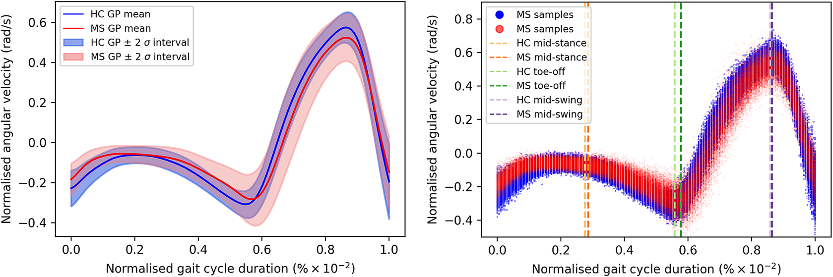
Visualization of the group differences. The solid white line shows the difference between the means of the two GPs, whereas the curved dashed lines showcase two standard deviations from the mean. The horizontal dashed line has been added here only for highlighting zero-crossing points. Notably, although the $ \pm 2\sigma $
interval may not seem symmetric above and below the mean upon initial observation, it is, in fact, symmetric. Disparities between the HC and MS models are highlighted across the input space using the MMD.
$ \pm 2\sigma $
interval may not seem symmetric above and below the mean upon initial observation, it is, in fact, symmetric. Disparities between the HC and MS models are highlighted across the input space using the MMD.

Direct comparison with other results presented in the relevant literature is challenging, as most of the characterizations of pathological gait primarily rely on joint kinematics, instead of segment kinematics. Nevertheless, in the case of the MS group, it is evident that the variability in the gait pattern progressively increases from mid-stance to mid-swing. Consistent with the findings of this study, other researchers have also reported greater variability in joint angles among individuals with MS, even among those with mild disability (Crenshaw et al., Reference Crenshaw, Royer, Richards and Hudson2006; Kelleher et al., Reference Kelleher, Spence, Solomonidis and Apatsidis2010; Nogueira et al., Reference Teixeira, Sabino, Filho, RMP and Thuler2013; Severini et al. Reference Severini, Manca, Ferraresi, Caniatti, Cosma, Baldasso, Straudi, Morelli and Basaglia2017). Similar trends have been found by Salehi et al. (Reference Salehi, Mofateh, Mehravar, Negahban, Tajali and Monjezi2020), where the authors reported significant differences between HC and MS during the stance and swing phase when looking at the deviation phase, as a measure of coordination variability. Additionally, the flatter trajectory observed during the stance phase may suggest a reduced range of plantar flexion, as reported by Nogueira et al. (Reference Teixeira, Sabino, Filho, RMP and Thuler2013). This reduction can lead to diminished power generation at the ankle, particularly during the initiation of the swing phase, potentially impacting the stability control throughout this latter phase. Such outcomes might be attributed to muscle weakness, spasticity, fatigue, or balance impairments (Nogueira et al., Reference Teixeira, Sabino, Filho, RMP and Thuler2013; Socie et al., Reference Socie, Sandroff, Pula, Hsiao-Wecksler, Motl and Sosnoff2013). Therefore, while confirming authors’ expectations, these group-level comparative results highlight the model’s ability to effectively capture the inherent variability of MS gait patterns, allowing for an informed analysis.
Next, to showcase the capabilities of the proposed hierarchical modeling approach to facilitate nuanced comparisons at lower levels in the hierarchy, individual gait pattern comparisons have been investigated, relative to the control group. This analysis aligns with the overarching aim of providing a patient-specific assessment. As such, detailed shank angular velocity predictions were generated for all participants in the study, which can be seen in Figure 8. Here, the held-out test data has been overlaid, allowing for enhanced insight into the model’s predictive performance. For clarity, the overlaid data corresponds to $ 30\% $
of randomly selected datapoints from each particular individual, which were not seen during training. The individual NMSE and MSLL scores are provided in Appendix F. Notably, individuals with MS exhibited significantly higher NMSE scores, indicating lower predictive capabilities of the MS model. Not surprisingly, the MS group also displayed significantly higher MSLL scores, further supporting the diminished predictive performance of the model for this population, given the increased variability in the gait patterns as well as the presence of asymmetry. To highlight individual-level discrepancies, samples drawn from the HC group predictive distribution were compared to samples drawn from the individual GPs, in a similar way to the MMD-based approach used above. More specifically, 500 samples were generated again at each of the 200 equidistant test locations along the input space, and the MMD was computed at every test location, for every subject. Then, the MMD values from all subjects were aggregated and normalized between 0 and 1. Therefore, the regions in the gait cycle which are most different relative to the control group are highlighted in Figure 9. As a result, while many of the PwMS appear to display a walking pattern closely aligned with the HC group pattern, with no immediate visible signs of impairment, several individuals with MS clearly stand out. However, it is important to acknowledge that comparing the individual MS predictions with the predictive distribution of the HC group is not sufficient. This is due to the presence of overlapping confidence intervals and comparable means shared between the HC group and the PwMS, stemming from the increased variability in the individual predictions of the latter group.
$ 30\% $
of randomly selected datapoints from each particular individual, which were not seen during training. The individual NMSE and MSLL scores are provided in Appendix F. Notably, individuals with MS exhibited significantly higher NMSE scores, indicating lower predictive capabilities of the MS model. Not surprisingly, the MS group also displayed significantly higher MSLL scores, further supporting the diminished predictive performance of the model for this population, given the increased variability in the gait patterns as well as the presence of asymmetry. To highlight individual-level discrepancies, samples drawn from the HC group predictive distribution were compared to samples drawn from the individual GPs, in a similar way to the MMD-based approach used above. More specifically, 500 samples were generated again at each of the 200 equidistant test locations along the input space, and the MMD was computed at every test location, for every subject. Then, the MMD values from all subjects were aggregated and normalized between 0 and 1. Therefore, the regions in the gait cycle which are most different relative to the control group are highlighted in Figure 9. As a result, while many of the PwMS appear to display a walking pattern closely aligned with the HC group pattern, with no immediate visible signs of impairment, several individuals with MS clearly stand out. However, it is important to acknowledge that comparing the individual MS predictions with the predictive distribution of the HC group is not sufficient. This is due to the presence of overlapping confidence intervals and comparable means shared between the HC group and the PwMS, stemming from the increased variability in the individual predictions of the latter group.
Individual predictions versus held-out test data. The first four rows correspond to HC individuals, while the last four rows correspond to PwMS.

Individual differences, MMD highlighted. The first four rows correspond to HC individuals, while the last four rows correspond to PwMS.
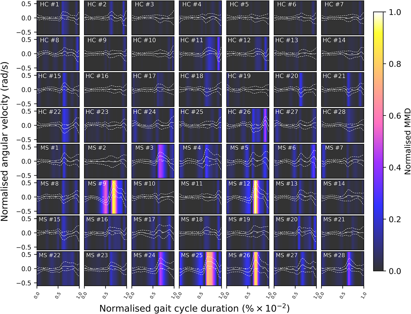
Figure 10 highlights the individual heteroscedastic variances, where departures from the contained HC gait patterns are evident for several individuals affected by MS, especially toward the termination of the stance and during the swing phase. Therefore, extending the hierarchical methodology to model individual gait patterns led to a novel feature that may serve as an indicator of the presence of neurological or musculoskeletal deficits. Two main factors are believed to be responsible for these results. The first one might be associated with the possible lack of control during the swing phase, as a result of muscle spasticity, fatigue or balance impairments (Nogueira et al., Reference Teixeira, Sabino, Filho, RMP and Thuler2013; Socie et al., Reference Socie, Sandroff, Pula, Hsiao-Wecksler, Motl and Sosnoff2013), while the second one pertains to the presence of asymmetry. For clarification, the alternative concept of asymmetry used here will be elaborated upon in the subsequent paragraphs, where the hierarchical model has been extended to include separate consideration for the left and right limbs. This extension has been added since the distribution over the outputs must be symmetric about the mean, which is not representative of the bi-modal distribution when asymmetry is present. However, the asymmetric gait patterns are still captured within the $ \pm 2\sigma $
bounds of the GP predictions. Thus, the variance predicted throughout the gait cycle could hold significant potential for integration into clinical gait analysis, noting that our methodology is not intended as a substitute for standard gait analysis, but rather as a valuable augmentation to the clinical assessment of patients with MS.
$ \pm 2\sigma $
bounds of the GP predictions. Thus, the variance predicted throughout the gait cycle could hold significant potential for integration into clinical gait analysis, noting that our methodology is not intended as a substitute for standard gait analysis, but rather as a valuable augmentation to the clinical assessment of patients with MS.
Heteroscedastic variance differences at the individual layer in the hierarchy, where data from the left and right limbs are combined for each individual. Each line corresponds to a single subject.

3.4. Quantifying individual asymmetry
In light of the results presented in Section 3.3, where the heteroscedastic variance has been observed to be one of the discriminant factors between HCs and PwMS, as well as considering the data normalization procedure, this section addresses the third objective of the case study concerning a novel proposal for asymmetry quantification. Recognizing asymmetry as one of the key factors for the increased variability in the gait patterns, the hierarchical model has been extended to separately address contralateral limbs. This extension not only allows for a nuanced exploration of contralateral limb data but also serves as a foundational step in introducing a novel methodology for quantifying lower limb asymmetry from a probabilistic perspective.
Traditionally, gait asymmetry has been defined as the absolute difference between the temporal metrics extracted from the left and right lower limbs (Godfrey et al., Reference Godfrey, Del Din, Barry, Mathers and Rochester2015) or as the natural logarithm of the absolute ratio of the shorter and the longer mean value of the temporal metric (Yogev et al., Reference Yogev, Plotnik, Peretz, Giladi and Hausdorff2007). Gait asymmetry is often considered to be an indicator of MS (Angelini et al., Reference Angelini, Buckley, Bonci, Radford, Sharrack, Paling, Nair and Mazza2021). However, in the context of this work, the term asymmetry is used to denote signals that align for the most part but display disparities at certain locations. To allow improved visual insights into the presence of asymmetry, the individual left and right model predictions are presented in Figure 11, relative to the unseen held-out test data.
Individual limb GP predictions. The first four rows correspond to HCs, while the last four rows correspond to PwMS. The solid lines represent the mean GP predictions, while the dotted lines correspond to the $ \pm 2\sigma $
interval. The dots represent the held-out test data.
$ \pm 2\sigma $
interval. The dots represent the held-out test data.
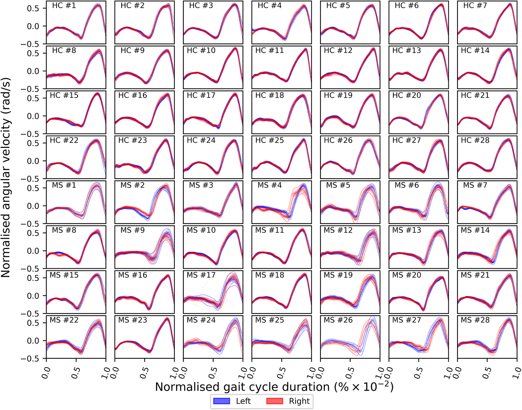
Analyzing Figure 11, disparities between left and right limbs for the MS-affected subject are evident, and several subjects clearly stand out. Conversely, the gait patterns observed for the HCs demonstrate a higher degree of symmetry, that is the same functional form throughout the gait cycle, despite the sparse presence of slight deviations between the left and right shanks (which can be considered negligible). Given the normalization procedure employed in this study, traditional asymmetry metrics can no longer be computed, necessitating the adoption of an alternative, comprehensive methodology. As such, first, the Wasserstein distance (Villani, Reference Villani2009) between samples drawn from each of the left and right limb GPs was computed across the input space. By computing the Wasserstein distance (WD) between these samples, a detailed insight into gait asymmetry can be obtained, effectively measuring how much the left and right limbs differ across the entire gait cycle. Similarly to the MMD distance, 500 samples were drawn from each GP’s predictive distributions at 100 equidistant points spread across the input space. Then, the WD was computed at each of the test locations (please refer to Figure G1 in Appendix G). This allows the end-users to visually discern the distinctive locations within the gait cycle where asymmetry is more prominent. Moreover, the overall effect of gait asymmetry was quantified by computing the area under the curve, thus providing a unified gait asymmetry metric. The comparison of the individual differences for all subjects included in the study can be seen in Figure 12a,b.
(a) HC, (b) MS—Unified Wasserstein distance computed between samples drawn from the left GP and the right GP for each of the individuals in both HC and MS groups. (c) Statistical comparison between the HC and MS groups.

Here, the PwMS numbered $ 2 $
,
$ 2 $
, $ 4 $
,
$ 4 $
, $ 19 $
,
$ 19 $
, $ 26 $
, and
$ 26 $
, and $ 27 $
particularly stand out. Subject
$ 27 $
particularly stand out. Subject $ 2 $
displayed a reduced range of mobility on the right shank during the stance phase, as well as an increased stance duration, when compared to the left leg. An uncontrolled movement was recorded on the right leg of subject
$ 2 $
displayed a reduced range of mobility on the right shank during the stance phase, as well as an increased stance duration, when compared to the left leg. An uncontrolled movement was recorded on the right leg of subject $ 4 $
. For this subject, the one-sided balance and coordination deficits were evident across the entire gait cycle, albeit more pronounced during the swing phase. Subject
$ 4 $
. For this subject, the one-sided balance and coordination deficits were evident across the entire gait cycle, albeit more pronounced during the swing phase. Subject $ 19 $
also displayed temporal differences between the left and right limbs. A reduced range of mobility was also recorded for subject
$ 19 $
also displayed temporal differences between the left and right limbs. A reduced range of mobility was also recorded for subject $ 26 $
for the right shank. This was recorded in conjunction with temporal differences between the two limbs, as well as increased variability during the swing phase and the end of the double support phase. Finally, subject
$ 26 $
for the right shank. This was recorded in conjunction with temporal differences between the two limbs, as well as increased variability during the swing phase and the end of the double support phase. Finally, subject $ 27 $
exhibited an uncontrolled right shank movement, accompanied by temporal differences as well as higher movement variability on the left leg. To summarize the asymmetry differences between the HC and MS groups, the nonparametric Mann–Whitney U test was employed, with a minimum significance alpha level of
$ 27 $
exhibited an uncontrolled right shank movement, accompanied by temporal differences as well as higher movement variability on the left leg. To summarize the asymmetry differences between the HC and MS groups, the nonparametric Mann–Whitney U test was employed, with a minimum significance alpha level of $ 5\% $
, highlighting statistically significant differences between the two groups (
$ 5\% $
, highlighting statistically significant differences between the two groups ( $ p<0.0001 $
, see Figure 12c). Nonetheless, the correlation between the WD and the clinical scores (in the form of the EDSS score) was also explored. Only a weak correlation has been found (
$ p<0.0001 $
, see Figure 12c). Nonetheless, the correlation between the WD and the clinical scores (in the form of the EDSS score) was also explored. Only a weak correlation has been found ( $ Pearso{n}^{\prime }s\;r=0.33 $
), which might suggest that asymmetry could manifest independently of disease severity in MS. Despite some arguments proposing a link between asymmetry and disease severity, such as Pau et al. (Reference Pau, Leban, Deidda, Putzolu, Porta, Coghe and Cocco2021), which demonstrated moderate correlations between joint kinematics asymmetry and the EDSS score using trend symmetry (Crenshaw and Richards, Reference Crenshaw and Richards2006), the findings of this study emphasize asymmetry relevance across various levels of MS disability. However, because of the considerably lower number of subjects included in the present study, drawing definitive clinical conclusions is not advisable.
$ Pearso{n}^{\prime }s\;r=0.33 $
), which might suggest that asymmetry could manifest independently of disease severity in MS. Despite some arguments proposing a link between asymmetry and disease severity, such as Pau et al. (Reference Pau, Leban, Deidda, Putzolu, Porta, Coghe and Cocco2021), which demonstrated moderate correlations between joint kinematics asymmetry and the EDSS score using trend symmetry (Crenshaw and Richards, Reference Crenshaw and Richards2006), the findings of this study emphasize asymmetry relevance across various levels of MS disability. However, because of the considerably lower number of subjects included in the present study, drawing definitive clinical conclusions is not advisable.
Second, an additional dimension of asymmetry analysis was pursued using the KL divergence. This process involved comparing the third-layer GP model that considers both limbs together with separate fourth-layer GP models that focus on the left and right limbs individually. This can be visualized in Figure 13a,b. The KL divergence, therefore, gives an indication of how well the combined model represents individual limb dynamics. A high KL divergence indicates that the combined model might not fully capture the nuances of each of the individual limbs, potentially reflecting asymmetry or distinctive characteristics. It should be noted that computing the KL divergence involves treating the GPs as multivariate Gaussian distributions and requires access to the full covariance matrix. In contrast to the previous asymmetry analysis employing the WD, analyzing the KL divergence metrics in Figure 13b, two additional MS subjects stand out, namely subjects $ 10 $
and
$ 10 $
and $ 14 $
. Although outcomes of subject
$ 14 $
. Although outcomes of subject $ 10 $
are not readily apparent, this result can be attributed to a subtle discrepancy between the left and right gait trajectories, which may elude visual inspection. Similar results were also recorded for subject
$ 10 $
are not readily apparent, this result can be attributed to a subtle discrepancy between the left and right gait trajectories, which may elude visual inspection. Similar results were also recorded for subject $ 14 $
, for which the presence of asymmetry was significantly more pronounced. The statistical comparison is presented in Figure 13c. The nonparametric Mann–Whitney U test was also employed in this case, with a minimum significance alpha level of
$ 14 $
, for which the presence of asymmetry was significantly more pronounced. The statistical comparison is presented in Figure 13c. The nonparametric Mann–Whitney U test was also employed in this case, with a minimum significance alpha level of $ 5\% $
, highlighting statistically significant differences between the two groups (
$ 5\% $
, highlighting statistically significant differences between the two groups ( $ p=0.0029 $
). However, no correlations between the KL divergence-based asymmetry metrics and EDSS score were found (
$ p=0.0029 $
). However, no correlations between the KL divergence-based asymmetry metrics and EDSS score were found ( $ Pearso{n}^{\prime }s\;r=0.1015 $
and
$ Pearso{n}^{\prime }s\;r=0.1015 $
and $ 0.0051 $
for the left and right shanks respectively), necessitating additional validation procedures before drawing any definitive clinical implications. However, the extension of the hierarchical model to individually consider contralateral limbs provided new insights into asymmetry levels in individuals affected by MS through a novel, multifaceted approach employing both the WD and the KL divergence as complementary asymmetry metrics. It is important to note that while the results presented here may suggest that asymmetry could be a challenging aspect of MS even in the early disease stages, caution should be exercised due to the small sample size and the need for further validation. Nonetheless, these insights may hold promise in assisting end-users toward providing improved personalized treatment or rehabilitation plans.
$ 0.0051 $
for the left and right shanks respectively), necessitating additional validation procedures before drawing any definitive clinical implications. However, the extension of the hierarchical model to individually consider contralateral limbs provided new insights into asymmetry levels in individuals affected by MS through a novel, multifaceted approach employing both the WD and the KL divergence as complementary asymmetry metrics. It is important to note that while the results presented here may suggest that asymmetry could be a challenging aspect of MS even in the early disease stages, caution should be exercised due to the small sample size and the need for further validation. Nonetheless, these insights may hold promise in assisting end-users toward providing improved personalized treatment or rehabilitation plans.
KL divergence computed between the individual level GP, combining the left and right limbs (third layer), and the individual limbs GP models, treating each limb individually (fourth layer). (a) HC, (b) MS. The lighter shade represents the left shank, while the darker shade represents the right shank. (c) statistical comparison.

While the advantages and potential applications of the newly proposed methodology for characterizing the shank angular velocity for PwMS have been emphasized, it is also important to consider its potential limitations. First, while the size of the inducing point set has been kept fixed and shared across all levels of the proposed hierarchy, in order to reduce the parameter space over which to optimize, future work should investigate how this design constraint affects the quality of the sparse approximation within the context of this work. Second, while the authors retained the entire dataset for the analysis proposed in this study, future work may also investigate the effects of downsampling and attempting the modeling problem with a reduced sample size. This may allow direct comparison of sparse GP approximations to standard GP regression.
In summary, the contribution of this work has been to propose a novel methodology for investigating similarities and differences in gait data across multiple hierarchical levels, presenting an initial case study of HVSHGPs directly applied to gait signals. The proposed approach is to make a departure from understanding gait with respect to a set of summary features; instead, the full gait cycle is modeled functionally, including varying noise/uncertainty throughout the signal. This model additionally obeys the underlying hierarchical structure of the gait data, exploiting similarities, but respecting differences. Finally, given that the shank angular velocity can be directly measured using wearable sensors—a cost-effective and versatile technology applicable in both laboratory and free-living environments—this signal presents a promising candidate for a biomarker in longitudinal studies of distal lower limb motion, offering advantages over traditional motion capture systems.
4. Conclusions
To the best of our knowledge, this study marks the first instance where scalable hierarchical GPs have been employed as a flexible Bayesian machine learning technique for modeling the nonlinear shank angular velocity. First, the hierarchical approach has been used to account for the temporally structured covariance between groups of patients and individual subjects. Then, the problem of scaling GPs to handle large datasets, such as the ones obtained during clinical gait assessments, has been addressed by using variational approximation methods. Finally, the variability in the gait cycle has been captured by input-dependent noise modeling, that is heteroscedasticity. This was achieved by modeling the log-noise variance of the process as an additional GP, which is also learnt in a variational manner. In possession of this hierarchical model is then possible to perform comparisons of the gait cycle across the full function space, rather than simply on a discrete feature level.
In conclusion, the move toward probabilistic modeling of the shank angular velocity allows for the use of probabilistic models, which offer robust and accurate mean predictions, along with automatic uncertainty estimates. The use of these models facilitates a better understanding of the impaired gait pattern in MS and also holds promise for possible extension to other pathological gait conditions.
Data availability statement
De-identified data underlying this study may be made available upon reasonable request to the corresponding author, subject to review approval by the relevant data access committees and under a suitable data sharing agreement.
Acknowledgments
We would like to acknowledge Ellen Buckley, Lorenza Angelini, Siva Nair, and David Paling for providing the data used in this study, which have been collected within the NIHR Sheffield Clinical Research Facility (CRF) as part of NIHR Sheffield Biomedical Research Centre (BRC) activities. We would like to thank all participants for giving their time to support this research.
Author contribution
Conceptualization: A.S., T.J.R., E.J.C., C.M.; Methodology: A.S, T.J.R.; Data curation: A.S.; Data visualization: A.S.; Writing original draft: A.S., T.J.R., E.J.C., C.M.; All authors approved the final submitted draft.
Funding statement
This study was funded by the National Institute for Health Research (NIHR) through the Sheffield Biomedical Research Centre (BRC, grant number IS-BRC-1215-20017) and PhD scholarship Grant no. 820820. Authors E.J. Cross and T.J. Rogers were supported by EP/W005816/1. T.J. Rogers is additionally supported by EP/W002140/1.
Competing interests
The authors declare none.
Ethical standard
The research meets all ethical guidelines, including adherence to the legal requirements of the study country.
Appendix A. Key standard GP equations
The reader should note the shorthand notation $ {K}_{XX} $
used to denote
$ {K}_{XX} $
used to denote $ k\left(X,X\right) $
throughout this appendix. Following the brief introduction to GPs in Section 2, the joint Gaussian distribution of the observed target values
$ k\left(X,X\right) $
throughout this appendix. Following the brief introduction to GPs in Section 2, the joint Gaussian distribution of the observed target values $ \boldsymbol{y} $
and the function values at test locations
$ \boldsymbol{y} $
and the function values at test locations $ {\boldsymbol{y}}_{\star } $
, under the prior is given by
$ {\boldsymbol{y}}_{\star } $
, under the prior is given by
 $$ \left[\begin{array}{c}\boldsymbol{y}\\ {}{\boldsymbol{y}}_{\star}\end{array}\right]\sim \mathcal{N}\left(\begin{array}{cc}\left[\begin{array}{c}m(X)\\ {}m\left({\boldsymbol{x}}_{\star}\right)\end{array}\right],& \left[\begin{array}{cc}{K}_{XX}+{\sigma}_n^2\unicode{x1D540}& {K}_{X{\boldsymbol{x}}_{\star }}\\ {}{K}_{{\boldsymbol{x}}_{\star}\boldsymbol{X}}& {K}_{{\boldsymbol{x}}_{\star }{\boldsymbol{x}}_{\star }}+{\sigma}_n^2\unicode{x1D540}\end{array}\right]\end{array}\right) $$
Here, $ X $
denotes a set of
$ X $
denotes a set of $ N $
,
$ N $
, $ D $
-dimensional training inputs, where
$ D $
-dimensional training inputs, where $ X\in {\mathrm{\mathbb{R}}}^{N\times D} $
, whereas
$ X\in {\mathrm{\mathbb{R}}}^{N\times D} $
, whereas $ \boldsymbol{y}\in {\mathrm{\mathbb{R}}}^{N\times 1} $
is the corresponding set of
$ \boldsymbol{y}\in {\mathrm{\mathbb{R}}}^{N\times 1} $
is the corresponding set of $ N $
measured training outputs. Given the training inputs
$ N $
measured training outputs. Given the training inputs $ X $
and their corresponding outputs
$ X $
and their corresponding outputs $ \boldsymbol{y} $
, the predictive distributions over
$ \boldsymbol{y} $
, the predictive distributions over $ {y}_{\star } $
at new test input locations
$ {y}_{\star } $
at new test input locations $ {\boldsymbol{x}}_{\star } $
are given by
$ {\boldsymbol{x}}_{\star } $
are given by
 $$ p\left({\boldsymbol{y}}_{\star }|{\boldsymbol{x}}_{\star },\boldsymbol{X},\boldsymbol{y}\right)\sim \mathcal{N}\left({\unicode{x1D53C}}_{Standard}\left[{\boldsymbol{y}}_{\star}\right],{\unicode{x1D54D}}_{Standard}\left[{\boldsymbol{y}}_{\star}\right]\right) $$
 $$ {\unicode{x1D53C}}_{Standard}\left[{\boldsymbol{y}}_{\star}\right]=m\left({\boldsymbol{x}}_{\star}\right)+{K}_{{\boldsymbol{x}}_{\star}\boldsymbol{X}}{\left({K}_{XX}+{\sigma}_n^2\unicode{x1D540}\right)}^{-1}\left(\boldsymbol{y}-m\left(\boldsymbol{x}\right)\right) $$
 $$ {\unicode{x1D54D}}_{Standard}\left[{\boldsymbol{y}}_{\star}\right]={K}_{{\boldsymbol{x}}_{\star }{\boldsymbol{x}}_{\star }}-{K}_{{\boldsymbol{x}}_{\star }X}{\left({K}_{XX}+{\sigma}_n^2\unicode{x1D540}\right)}^{-1}{K}_{X{\boldsymbol{x}}_{\star }}+{\sigma}_n^2\unicode{x1D540} $$
The kernel hyperparameters can be found via the following optimization of the negative log marginal likelihood:
 $$ \hat{\boldsymbol{\theta}}=\underset{\theta }{\arg \min }-\log p\left(\boldsymbol{y}|\boldsymbol{x},\boldsymbol{\theta} \right) $$
with
 $$ {\displaystyle \begin{array}{c}-\log p\left(\boldsymbol{y}|\boldsymbol{x},\boldsymbol{\theta} \right)=-\log \mathcal{N}\left(\boldsymbol{y}|m\left(\boldsymbol{x}\right),{K}_{XX}+{\sigma}_n^2\unicode{x1D540}\right)\\ {}=\underset{constant\hskip0.35em \mathrm{term}}{\underbrace{\frac{N}{2}\log \left(2\pi \right)}}+\underset{complexity\hskip0.35em \mathrm{term}}{\underbrace{\frac{1}{2}\log \mid {K}_{XX}+{\sigma}_n^2\unicode{x1D540}\mid }}+\underset{model\hskip0.35em \mathrm{fit}\hskip0.35em \mathrm{term}}{\underbrace{\frac{1}{2}\left({\left(\boldsymbol{y}-m\left(\boldsymbol{x}\right)\right)}^T{\left({K}_{XX}+{\sigma}_n^2\unicode{x1D540}\right)}^{-1}\left(\boldsymbol{y}-m\left(\boldsymbol{x}\right)\right)\right)}}\end{array}} $$
The annotated terms in Equation 18 have readily available interpretations, and it can be clearly seen that there is a trade-off between model fit and model complexity. This property is known as the Bayesian Occam’s Razor (Rasmussen and Ghahramani, Reference Rasmussen and Ghahramani2001; Rasmussen and Williams, Reference Rasmussen and Williams2006). Thus, the hyperparameters of the kernel can be learnt and the GP is completely defined by Equations 15 and 16.
Appendix B. Key sparse GP equations
Following the introduction presented in Section 2.1, the key equations required for variational approximation methods are presented here. Briefly, variational inference methods derive a lower bound of the log-marginal likelihood using a distribution $ q(f) $
over the entire infinite-dimensional function:
$ q(f) $
over the entire infinite-dimensional function:
 $$ \log p\left(\boldsymbol{y}|\boldsymbol{\theta} \right)=\log \int p\left(\boldsymbol{y},f|\boldsymbol{\theta} \right) df\ge \int q(f)\log \frac{p\left(\boldsymbol{y},f|\boldsymbol{\theta} \right)}{q(f)} df={\unicode{x1D53C}}_{q(f)}\left[\log \frac{p\left(\boldsymbol{y},f|\boldsymbol{\theta} \right)}{q(f)}\right]={F}_{Sparse}\left(q,\boldsymbol{\theta} \right) $$
This lower bound $ {F}_{Sparse} $
can be expressed in terms of the KL divergence between the variational distribution and the true posterior:
$ {F}_{Sparse} $
can be expressed in terms of the KL divergence between the variational distribution and the true posterior:
 $$ {F}_{Sparse}\left(q,\boldsymbol{\theta} \right)={\unicode{x1D53C}}_q\left[\log p\left(\boldsymbol{y}|\boldsymbol{\theta} \right)\right]- KL\left(q(f)\Big\Vert p\left(f|\boldsymbol{y},\boldsymbol{\theta} \right)\right) $$
Given the set of inducing points $ \left\{Z,\boldsymbol{u}\right\} $
, where
$ \left\{Z,\boldsymbol{u}\right\} $
, where $ Z $
contains the locations of the inducing points and
$ Z $
contains the locations of the inducing points and $ \boldsymbol{u} $
are the values of the latent functions at these points, the variational lower bound can be written explicitly as
$ \boldsymbol{u} $
are the values of the latent functions at these points, the variational lower bound can be written explicitly as
 $$ {\displaystyle \begin{array}{c}{F}_{Sparse}(Z)=-\frac{1}{2}\log \left(2\pi \right)-\frac{1}{2}\log \mid {Q}_{XX}+{\sigma}_n^2\unicode{x1D540}\mid -\frac{1}{2}{\left(\boldsymbol{y}-m(X)\right)}^T{\left[{Q}_{XX}+{\sigma}_n^2\unicode{x1D540}\right]}^{-1}\left(\boldsymbol{y}-m(X)\right)\\ {}-\frac{1}{2}{\sigma}_n^{-2} tr\left({K}_{XX}-{Q}_{XX}\right)\end{array}} $$
where $ tr\left(\cdot \right) $
is the trace operator and
$ tr\left(\cdot \right) $
is the trace operator and $ {Q}_{XX} $
is the approximate covariance matrix, defined as
$ {Q}_{XX} $
is the approximate covariance matrix, defined as
 $$ {Q}_{XX}={K}_{X\boldsymbol{u}}{K}_{\boldsymbol{u}\boldsymbol{u}}^{-1}{K}_{\boldsymbol{u}X} $$
Here, the kernel functions, evaluated at the data points $ X $
, inducing input points
$ X $
, inducing input points $ Z $
, and between the data and inducing points, are represented by the kernel matrices
$ Z $
, and between the data and inducing points, are represented by the kernel matrices $ {K}_{XX} $
,
$ {K}_{XX} $
, $ {K}_{\boldsymbol{uu}} $
and
$ {K}_{\boldsymbol{uu}} $
and $ {K}_{X\boldsymbol{u}} $
, respectively. Please note, that according to Titsias, Reference Titsias2009; Bui et al. (Reference Bui, Yan and Turner2017), the notation used here can be generalized, such that:
$ {K}_{X\boldsymbol{u}} $
, respectively. Please note, that according to Titsias, Reference Titsias2009; Bui et al. (Reference Bui, Yan and Turner2017), the notation used here can be generalized, such that:
 $$ {Q}_{\boldsymbol{ab}}={K}_{\boldsymbol{au}}{K}_{\boldsymbol{uu}}^{-1}{K}_{\boldsymbol{ub}} $$
The bound derived in Equation 21 can then be used for hyperparameter optimization. For the complete derivation of this bound, the reader is referred to Michalis (Reference Michalis2009). Following optimization, predictions can be done in a comparable manner to the standard GP. Hence, the predictive distribution is given by (It should be noted that the explicit conditioning of the posteriors on the training data, test input, inducing points, and hyperparameters was dropped here for simplicity of notation.)
 $$ p\left({\boldsymbol{y}}_{\star }|{\boldsymbol{x}}_{\star },X,\boldsymbol{y},\boldsymbol{u}\right)=\mathcal{N}\left({\unicode{x1D53C}}_{Sparse}\left[{\boldsymbol{y}}_{\star}\right],{\unicode{x1D54D}}_{Sparse}\left[{\boldsymbol{y}}_{\star}\right]\right) $$
 $$ {\unicode{x1D53C}}_{Sparse}\left[{\boldsymbol{y}}_{\star}\right]={Q}_{{\boldsymbol{x}}_{\star }X}{\left({Q}_{XX}+{\sigma}_n^2\unicode{x1D540}\right)}^{-1}\boldsymbol{y} $$
 $$ {\unicode{x1D54D}}_{Sparse}\left[{\boldsymbol{y}}_{\star}\right]={K}_{{\boldsymbol{x}}_{\star }{\boldsymbol{x}}_{\star }}-{Q}_{{\boldsymbol{x}}_{\star }X}{\left({Q}_{XX}+{\sigma}_n^2\unicode{x1D540}\right)}^{-1}{Q}_{{\boldsymbol{Xx}}_{\star }} $$
The main benefit of this sparse approximation is that the computational requirements are reduced from $ \mathcal{O}\left({N}^3\right) $
to
$ \mathcal{O}\left({N}^3\right) $
to $ \mathcal{O}\left({NM}^2\right) $
for
$ \mathcal{O}\left({NM}^2\right) $
for $ M $
inducing points. Naively, it is not clear where the computational speed-up is found. However, note that the Woodbury inversion lemma can be applied as detailed below:
$ M $
inducing points. Naively, it is not clear where the computational speed-up is found. However, note that the Woodbury inversion lemma can be applied as detailed below:
 $$ {\displaystyle \begin{array}{c}{\left({Q}_{XX}+{\sigma}_n^2\unicode{x1D540}\right)}^{-1}=\\ {}{\left({K}_{Xu}{K}_{uu}^{-1}{K}_{uX}+{\sigma}_n^2\unicode{x1D540}\right)}^{-1}=\\ {}{\sigma}_n^{-2}\unicode{x1D540}-{\sigma}_n^{-2}\unicode{x1D540}\underset{{\mathrm{\mathbb{R}}}^{M\times M}}{\underbrace{{\left({K}_{uu}+{K}_{uX}\left({\sigma}_n^{-2}\unicode{x1D540}\right){K}_{Xu}\right)}^{-1}}}{K}_{uX}{\sigma}_n^{-2}\unicode{x1D540}\end{array}} $$
Appendix C. Key heteroscedastic GP equations
The heteroscedastic lower bound is given by Equation 26, as follows:
 $$ {F}_{Heteroscedastic}\left(\boldsymbol{\mu}, \Sigma \right)=\log \mathcal{N}\left(\boldsymbol{y}|\mathbf{0},{K}_f+R\right)-\frac{1}{4} tr\left(\Sigma \right)- KL\left(\mathcal{N}\left(\boldsymbol{h}|\boldsymbol{\mu}, \Sigma \right)\Big\Vert \mathcal{N}\left(\boldsymbol{h}|{\mu}_0\mathbf{1},{K}_h\right)\right) $$
To ensure clear notation, $ {K}_f $
and
$ {K}_f $
and $ {K}_h $
are used here to denote the covariance matrices of the two GPs used to model
$ {K}_h $
are used here to denote the covariance matrices of the two GPs used to model $ f\left(\boldsymbol{x}\right) $
and
$ f\left(\boldsymbol{x}\right) $
and $ h\left(\boldsymbol{x}\right) $
, respectively.
$ h\left(\boldsymbol{x}\right) $
, respectively. $ R $
is a diagonal matrix whose elements are
$ R $
is a diagonal matrix whose elements are $ {R}_{ii}=\exp \left({\boldsymbol{\mu}}_i-0.5{\Sigma}_{ii}\right) $
. Moreover,
$ {R}_{ii}=\exp \left({\boldsymbol{\mu}}_i-0.5{\Sigma}_{ii}\right) $
. Moreover, $ \boldsymbol{\mu} $
and
$ \boldsymbol{\mu} $
and $ \Sigma $
are the variational parameters to be determined, defined according to Equation 27, for some positive semidefinite diagonal matrix
$ \Sigma $
are the variational parameters to be determined, defined according to Equation 27, for some positive semidefinite diagonal matrix $ \Lambda $
(see Liu et al., Reference Liu, Ong and Cai2018):
$ \Lambda $
(see Liu et al., Reference Liu, Ong and Cai2018):
 $$ \boldsymbol{\mu} ={K}_h\left(\Lambda -\frac{1}{2}\unicode{x1D540}\right)\mathbf{1}+{\mu}_0\mathbf{1}, $$
 $$ {\Sigma}^{-1}={K}_h^{-1}+\Lambda $$
It can be seen that this implementation requires the optimization of $ N+N\left(N+1\right)/2 $
free variational parameters. This is achieved through the reparametrization of
$ N+N\left(N+1\right)/2 $
free variational parameters. This is achieved through the reparametrization of $ \boldsymbol{\mu} $
and
$ \boldsymbol{\mu} $
and $ \Sigma $
in terms of
$ \Sigma $
in terms of $ \Lambda $
(Lázaro-Gredilla and Titsias, Reference Lázaro-Gredilla and Titsias2011). As a result, the computational complexity is roughly twice that of the homoscedastic GP.
$ \Lambda $
(Lázaro-Gredilla and Titsias, Reference Lázaro-Gredilla and Titsias2011). As a result, the computational complexity is roughly twice that of the homoscedastic GP.
Another challenge that has emerged from the use of a heteroscedastic GP is the lack of a complete predictive distribution in a closed form. Fortunately, it is still possible to approximate the first two moments (that is the mean and variance) of the predictive distribution. These are expressed in the following equations:
 $$ {\unicode{x1D53C}}_q\left[{\boldsymbol{y}}_{\star}\right]={\boldsymbol{a}}_{\star } $$
 $$ {\unicode{x1D54D}}_q\left[{\boldsymbol{y}}_{\star}\right]={{\boldsymbol{c}}_{\star}}^2+\exp \left({\boldsymbol{\mu}}_{\star }+\frac{1}{2}{\sigma_{\star}}^2\right) $$
Here, the following notations have been used:
 $$ {\boldsymbol{a}}_{\star }={k}_f\left({x}_{\star },X\right){\left({K}_f+R\right)}^{-1}\boldsymbol{y} $$
 $$ {{\boldsymbol{c}}_{\star}}^2={k}_f\left({\boldsymbol{x}}_{\star },{\boldsymbol{x}}_{\star}\right)-{k}_f\left({\boldsymbol{x}}_{\star },X\right)\left({\left({K}_f+R\right)}^{-1}\right){k}_f\left(X,{\boldsymbol{x}}_{\star}\right) $$
 $$ {\boldsymbol{\mu}}_{\star }={k}_h\left({\boldsymbol{x}}_{\star },X\right)\left(\Lambda -\frac{1}{2}\unicode{x1D540}\right)\mathbf{1}+{\mu}_0 $$
 $$ {\sigma_{\star}}^2={k}_h\left({\boldsymbol{x}}_{\star },{\boldsymbol{x}}_{\star}\right)-{k}_h\left({\boldsymbol{x}}_{\star },X\right){\left({K}_h+{\Lambda}^{-1}\right)}^{-1}{k}_h\left(X,{\boldsymbol{x}}_{\star}\right) $$
With these definitions, it is now possible to make predictions using a heteroscedastic GP. Here, it is assumed that the first two moments presented above are representative of the true underlying distribution.
Appendix D. Key variational sparse heteroscedastic GP equations
In this section, the covariance matrices are indexed by a superscript $ f $
or
$ f $
or $ h $
, which denotes the function and corresponding hyperparameters under consideration. The subscripts denote which sets of points the covariance is computed between, with
$ h $
, which denotes the function and corresponding hyperparameters under consideration. The subscripts denote which sets of points the covariance is computed between, with $ X $
being the full set of points and
$ X $
being the full set of points and $ u $
being the set of inducing points for the corresponding function. Therefore, as an example,
$ u $
being the set of inducing points for the corresponding function. Therefore, as an example, $ {K}_{Xu}^h $
is the covariance matrix between the training points and the inducing points for
$ {K}_{Xu}^h $
is the covariance matrix between the training points and the inducing points for $ h\left(\boldsymbol{x}\right) $
, given the hyperparameters of the kernel for the log-noise GP. Although there is a nontrivial amount of algebra to arrive at these equations, to learn the optimal set of hyperparameters for the VSHGP model, the problem reduces to maximizing the following lower bound (Liu et al., Reference Liu, Ong and Cai2018), which is defined as
$ h\left(\boldsymbol{x}\right) $
, given the hyperparameters of the kernel for the log-noise GP. Although there is a nontrivial amount of algebra to arrive at these equations, to learn the optimal set of hyperparameters for the VSHGP model, the problem reduces to maximizing the following lower bound (Liu et al., Reference Liu, Ong and Cai2018), which is defined as
 $$ {\displaystyle \begin{array}{c}{F}_{Sparse\hbox{-} Heteroscedastic}\left(\boldsymbol{\mu}, \Sigma \right)=\mathrm{log}\mathcal{N}\left(\boldsymbol{y}|\mathbf{0},{Q}_{XX}^f+{R}_h\right)-0.25 Tr\left[{\Sigma}_h\right]\\ {}-0.5 Tr\left[{R}_h^{-1}\left({K}_{XX}^f-{Q}_{XX}^f\right)\right]- KL\left(\mathcal{N}\left(\boldsymbol{h}|{\boldsymbol{\mu}}_{\boldsymbol{u}},{\Sigma}_u\right)\Big\Vert \mathcal{N}\left(\boldsymbol{h}|{\mu}_0,{K}_{uu}^h\right)\right)\end{array}} $$
where the diagonal matrix $ {R}_h\in {\mathrm{\mathbb{R}}}^{N\times N} $
is defined as:
$ {R}_h\in {\mathrm{\mathbb{R}}}^{N\times N} $
is defined as: $ {R}_{ii}=\exp \left({\boldsymbol{\mu}}_{\boldsymbol{h}i}-0.5{\Sigma}_{hii}\right) $
, with the mean and variance.
$ {R}_{ii}=\exp \left({\boldsymbol{\mu}}_{\boldsymbol{h}i}-0.5{\Sigma}_{hii}\right) $
, with the mean and variance.
 $$ {\boldsymbol{\mu}}_{\boldsymbol{h}}={\Omega}_{Xu}^h\left({\boldsymbol{\mu}}_{\boldsymbol{u}}-{\mu}_0\mathbf{1}\right)+{\mu}_0\mathbf{1} $$
 $$ {\Sigma}_h={K}_{XX}^h-{Q}_{XX}^h+{\Omega}_{Xu}^h{\Sigma}_u{\left({\Omega}_{Xu}^h\right)}^T $$
 $$ {\boldsymbol{\mu}}_{\boldsymbol{u}}={K}_{uX}^h\left(\Lambda -0.5\unicode{x1D540}\right)\mathbf{1}+{\mu}_0\mathbf{1} $$
 $$ {\Sigma}_u^{-1}={\left({K}_{uu}^h\right)}^{-1}+{\left({\Omega}_{Xu}^h\right)}^T{\Lambda \Omega}_{Xu}^h $$
Here, $ \Lambda $
is a positive semi-definite diagonal matrix, and
$ \Lambda $
is a positive semi-definite diagonal matrix, and $ {\Omega}_{Xu}^h $
is defined according to Equation 32. For details regarding the full derivation, the reader is referred to Liu et al. (Reference Liu, Ong and Cai2018).
$ {\Omega}_{Xu}^h $
is defined according to Equation 32. For details regarding the full derivation, the reader is referred to Liu et al. (Reference Liu, Ong and Cai2018).
 $$ {\Omega}_{Xu}^h={K}_{Xu}^h{\left({K}_{uu}^h\right)}^{-1} $$
The sparse approximation for the two GPs employed to model the heteroscedastic noise introduces several additional hyperparameters associated with the inducing points used in $ f\left(\boldsymbol{x}\right) $
and
$ f\left(\boldsymbol{x}\right) $
and $ h\left(\boldsymbol{x}\right) $
. It should be noted that the number of inducing points does not necessarily have to be equal for both functions. As a result of the introduction of the two sets of inducing points, the number of hyperparameters has now increased to include the kernel hyperparameters for
$ h\left(\boldsymbol{x}\right) $
. It should be noted that the number of inducing points does not necessarily have to be equal for both functions. As a result of the introduction of the two sets of inducing points, the number of hyperparameters has now increased to include the kernel hyperparameters for $ {k}_f\left(\boldsymbol{x},{\boldsymbol{x}}^{\prime}\right) $
and
$ {k}_f\left(\boldsymbol{x},{\boldsymbol{x}}^{\prime}\right) $
and $ {k}_h\left(\boldsymbol{x},{\boldsymbol{x}}^{\prime}\right) $
, the constant mean for the log noise variance,
$ {k}_h\left(\boldsymbol{x},{\boldsymbol{x}}^{\prime}\right) $
, the constant mean for the log noise variance, $ {\mu}_0 $
, the location of the
$ {\mu}_0 $
, the location of the $ m $
inducing points for
$ m $
inducing points for $ f\left(\boldsymbol{x}\right) $
, the location of the
$ f\left(\boldsymbol{x}\right) $
, the location of the $ u $
inducing points for
$ u $
inducing points for $ h\left(\boldsymbol{x}\right) $
, as well as the
$ h\left(\boldsymbol{x}\right) $
, as well as the $ n $
variational parameters composing the
$ n $
variational parameters composing the $ \Lambda $
diagonal matrix.
$ \Lambda $
diagonal matrix.
However, as with the non-sparse heteroscedastic GP, computing the predictive distribution $ p\left({\boldsymbol{y}}_{\star }|\boldsymbol{y},{\boldsymbol{x}}_{\star}\right) $
at the test points
$ p\left({\boldsymbol{y}}_{\star }|\boldsymbol{y},{\boldsymbol{x}}_{\star}\right) $
at the test points $ {\boldsymbol{x}}_{\star } $
requires marginalizing over the latent noise process, leading to an intractable integral. This marginalization implies that the predictive posterior is no longer Gaussian. In practice, following Lázaro-Gredilla and Titsias (Reference Lázaro-Gredilla and Titsias2011) and Liu et al. (Reference Liu, Ong and Cai2018), we can approximate the predictive distribution by matching its first two moments via Gauss–Hermite quadrature. This procedure yields an approximate Gaussian predictive distribution with mean
$ {\boldsymbol{x}}_{\star } $
requires marginalizing over the latent noise process, leading to an intractable integral. This marginalization implies that the predictive posterior is no longer Gaussian. In practice, following Lázaro-Gredilla and Titsias (Reference Lázaro-Gredilla and Titsias2011) and Liu et al. (Reference Liu, Ong and Cai2018), we can approximate the predictive distribution by matching its first two moments via Gauss–Hermite quadrature. This procedure yields an approximate Gaussian predictive distribution with mean $ {\mu}_{\star } $
and variance
$ {\mu}_{\star } $
and variance $ {\sigma}_{\star}^{\mathbf{2}} $
as follows:
$ {\sigma}_{\star}^{\mathbf{2}} $
as follows:
 $$ {\boldsymbol{\mu}}_{\star }={\boldsymbol{\mu}}_{\star}^f,\hskip0.4em {\sigma}_{\star}^2={{\sigma_{\star}}^f}^2+{e}^{{{\boldsymbol{\mu}}_{\star}}^h+{{\sigma_{\star}}^h}^2/2} $$
where
 $$ {{\boldsymbol{\mu}}_{\star}}^f={K}_{\star u}^f{K}_R^{-1}{K}_{uX}^f{R}_h^{-1}y, $$
 $$ {{\sigma_{\star}}^f}^2={K}_{\star \star}^f-{K}_{\star u}^f{\left({K}_{uu}^f\right)}^{-1}{K}_{u\star}^f+{K}_{\star u}^f{K}_R^{-1}{k}_{u\star}^f, $$
 $$ {{\sigma_{\star}}^h}^2={K}_{\star \star}^h-{K}_{\star u}^h{\left({K}_{uu}^h\right)}^{-1}{K}_{u\star}^h+{K}_{\star u}^h{K}_{\Lambda}^{-1}{K}_{u\star}^h, $$
 $$ {K}_R={K}_{uX}^f{R}_h^{-1}{K}_{Xu}^f+{K}_{uu}^f $$
 $$ {K}_{\Lambda}={K}_{uX}^h{\Lambda}^{-1}{K}_{Xu}^h+{K}_{uu}^h $$
Here, it is important to note that the correction term, $ {K}_{\star u}^f{K}_R^{-1}{K}_{u\star}^f $
in Equation 34b contains the heteroscedasticity information from the noise term
$ {K}_{\star u}^f{K}_R^{-1}{K}_{u\star}^f $
in Equation 34b contains the heteroscedasticity information from the noise term $ {R}_h $
.
$ {R}_h $
.
Appendix E. Group and individual model comparisons using the KL divergence
Figure E1 demonstrates the asymmetric nature of the Kullback–Leibler (KL) divergence when comparing group-level differences across the gait cycle. The left panel shows the divergence pattern when using the healthy control group as the reference distribution, while the right panel shows the same comparison with the MS group as the reference. The distinct patterns between these two panels highlight a key limitation of KL divergence: its asymmetric property leads to different interpretations depending on the choice of reference distribution. In addition to this, it is clear that the KL divergence is disproportionately sensitive to small values in the reference distribution rather than capturing the absolute magnitude of differences. As such, both visualizations show notable dissimilarities in the first $ 15\% $
, the range of
$ 15\% $
, the range of $ 35 $
to
$ 35 $
to $ 55\% $
, and the range of
$ 55\% $
, and the range of $ 60 $
to
$ 60 $
to $ 90\% $
of the gait cycle, but with different magnitudes and temporal distributions, emphasizing why a symmetric metric like the Maximum Mean Discrepancy (MMD) might be preferable for clinical interpretations (see Section 3.3). This same analysis is extended to individual-level comparisons against the control group, as shown in Figure E2.
$ 90\% $
of the gait cycle, but with different magnitudes and temporal distributions, emphasizing why a symmetric metric like the Maximum Mean Discrepancy (MMD) might be preferable for clinical interpretations (see Section 3.3). This same analysis is extended to individual-level comparisons against the control group, as shown in Figure E2.
Comparison of GP posterior distributions using KL divergence. (Left) KL divergence computed using the healthy control (HC) group GP posterior as the reference distribution. (Right) KL divergence computed using the MS group GP posterior as the reference distribution. The solid white line represents the mean difference between the two GPs, while the dashed lines indicate the $ \pm 2\sigma $
uncertainty bounds of the difference.
$ \pm 2\sigma $
uncertainty bounds of the difference.

Comparison of individual differences using KL divergence. (Top) KL divergence computed using the healthy control (HC) group GP posterior as the reference distribution. (Bottom) KL divergence computed using individual-specific posteriors as reference distributions. The first four rows represent HC individuals, while the last four rows represent people with MS (PwMS). Higher values (yellow) indicate greater divergence between distributions.

Appendix F. Individual models: Performance metrics
The individual model (aggregating contralateral limb data) performance metrics are presented in Table F1.
Performance metrics of individual models aggregating contralateral limb data
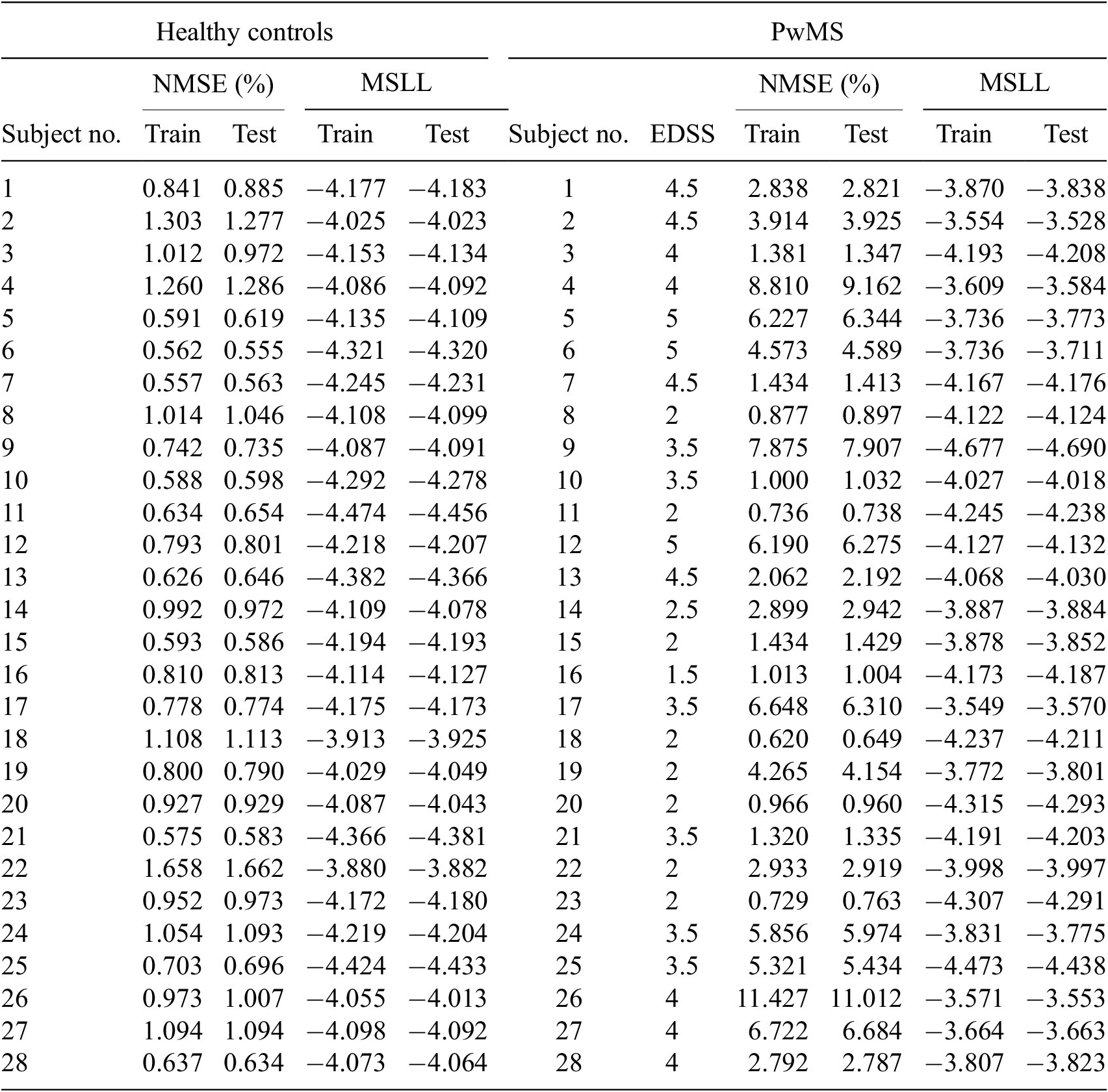
Appendix G. Wasserstein asymmetry
Figure G1 displays the distinctive locations across the entire gait cycle where asymmetry is present in the gait patterns obtained from the individual limb models, that is left versus right. Here, each individual line corresponds to a unique individual.
Wasserstein distance computed between left and right limb models.

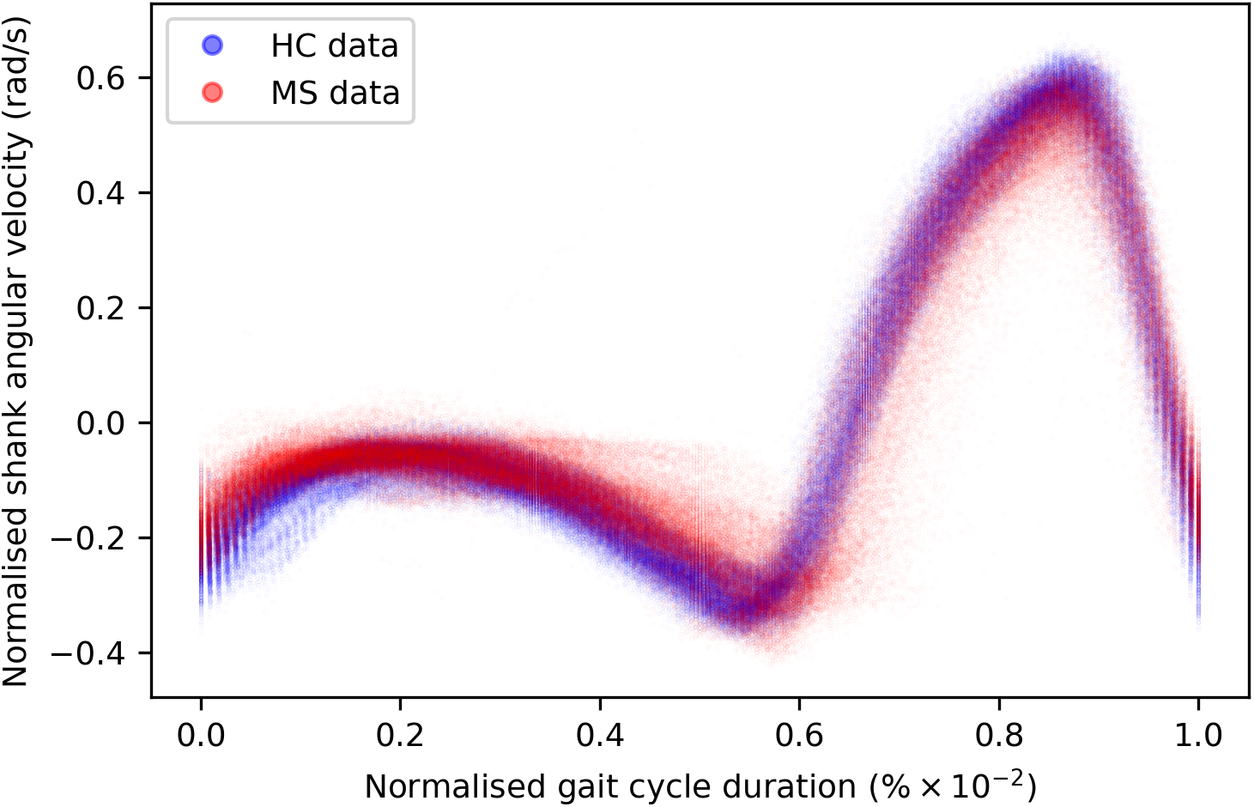


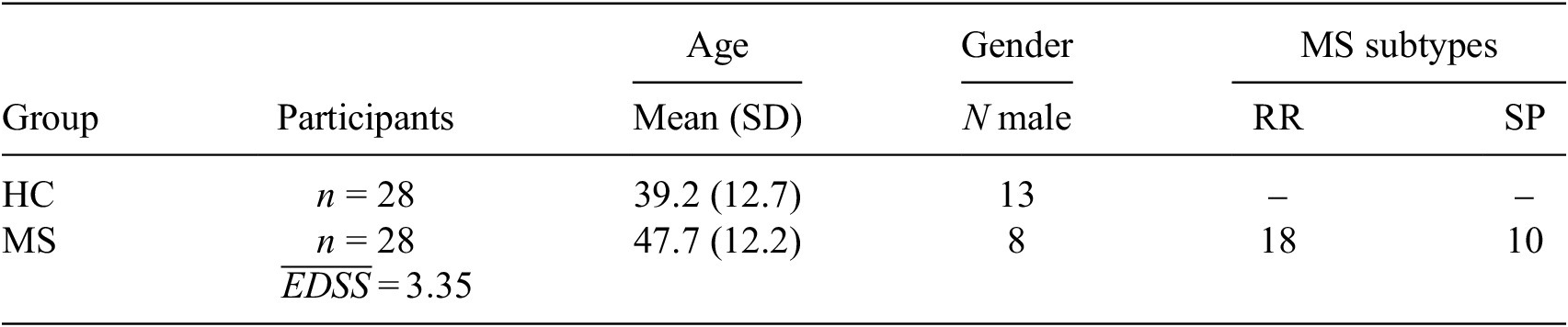
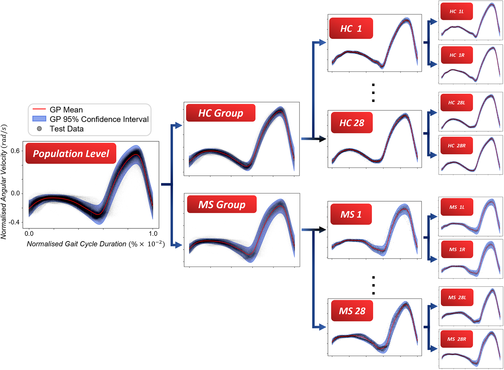
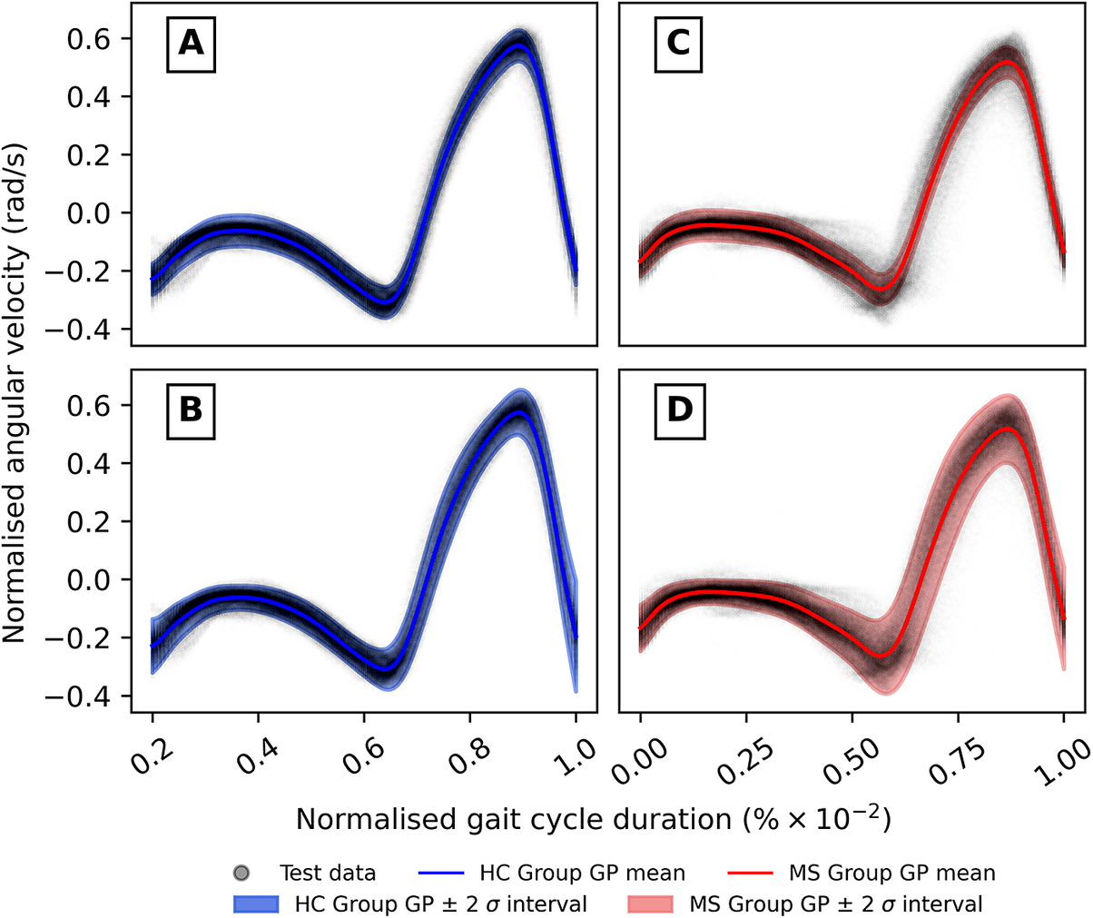
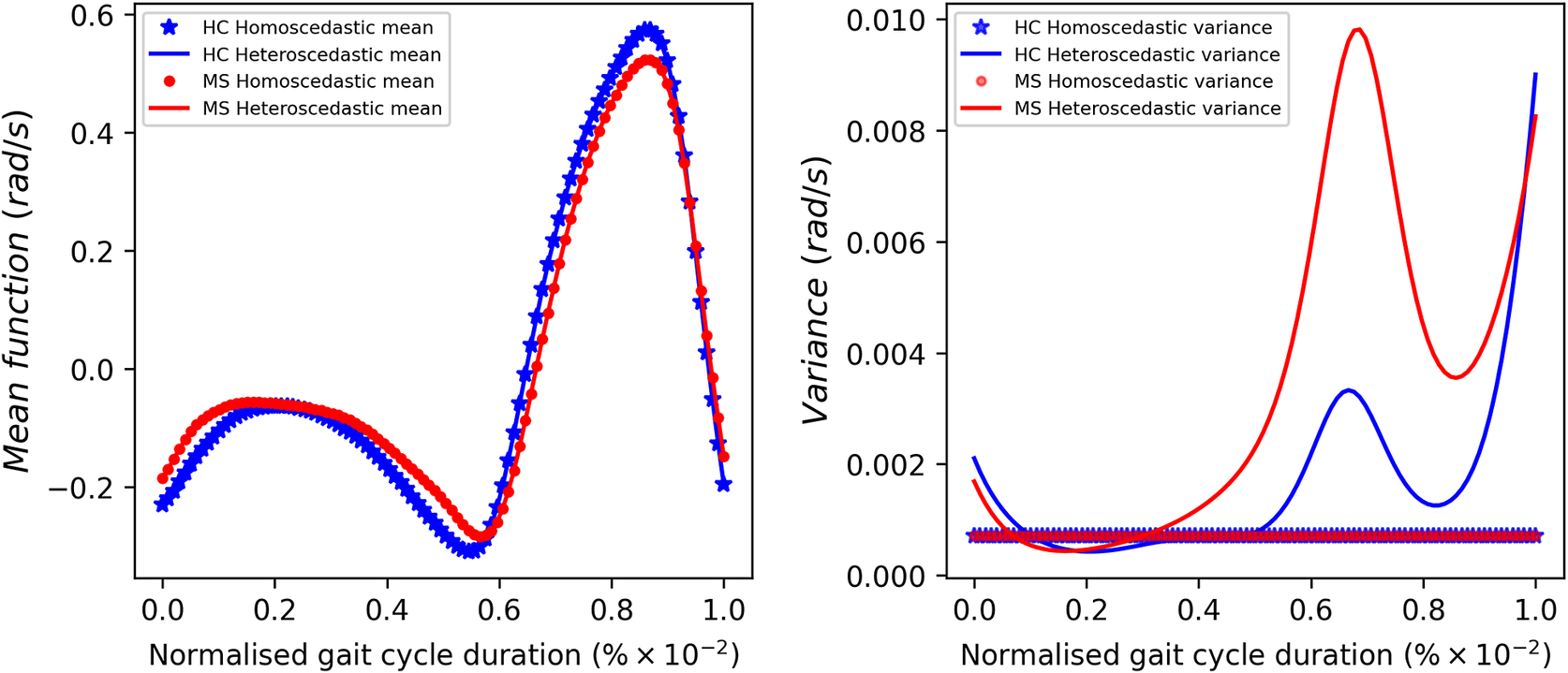
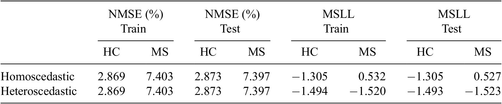

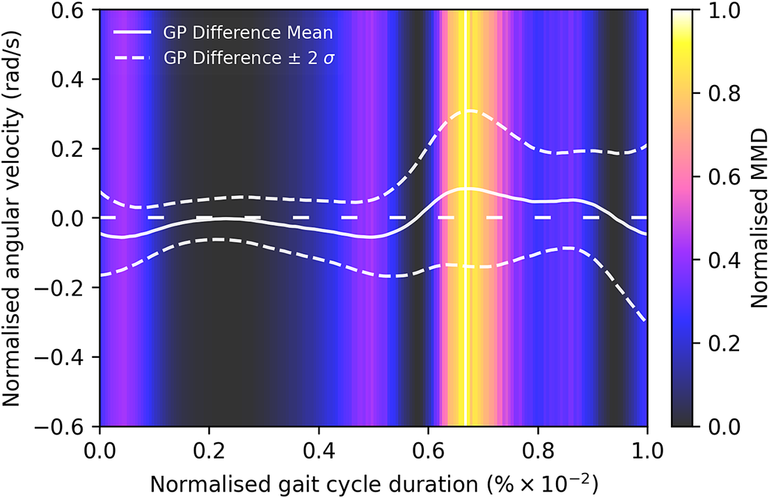

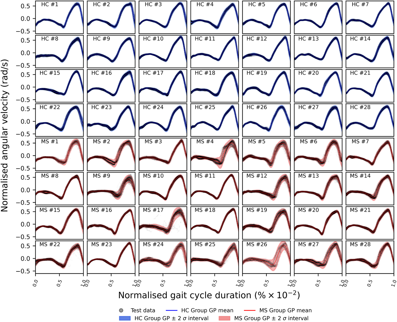

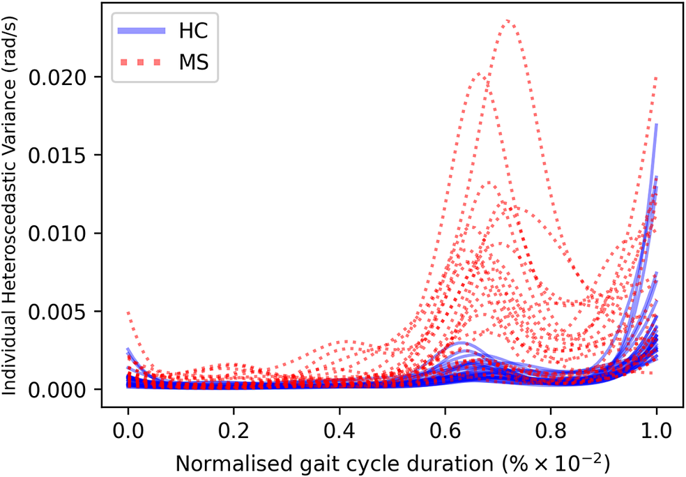


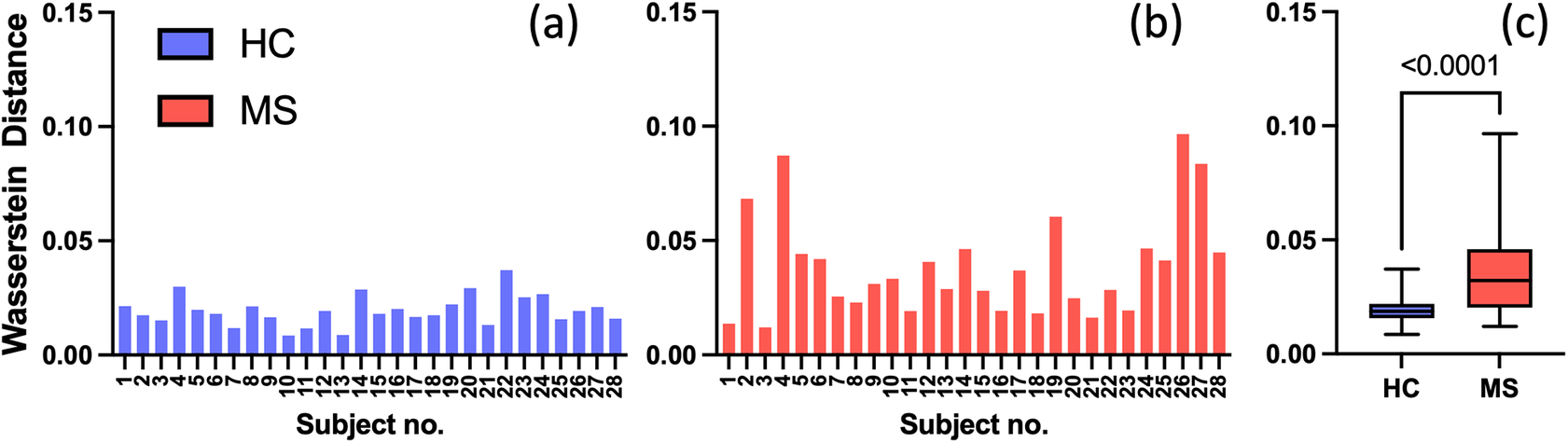
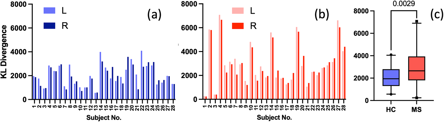
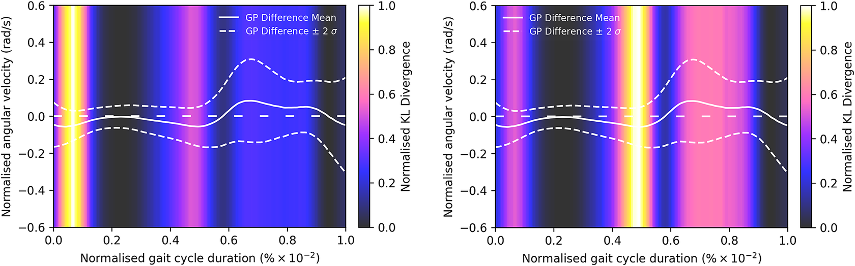

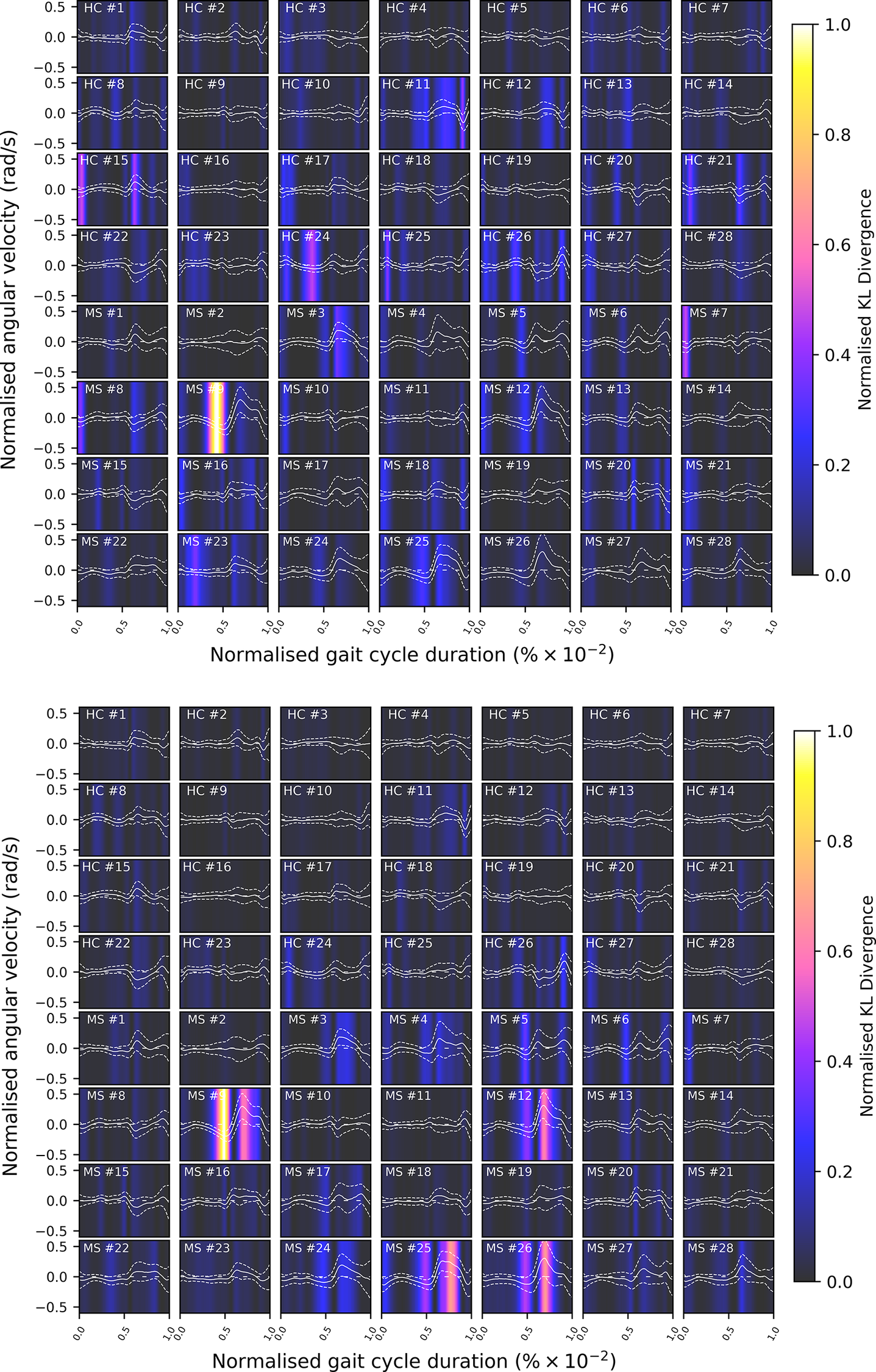

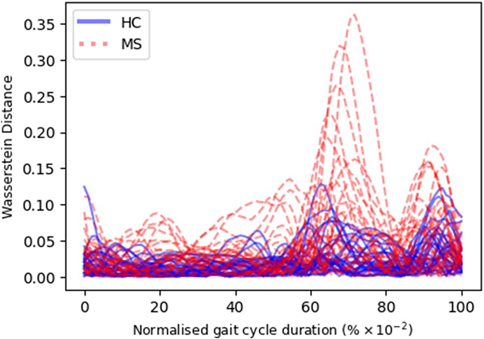

 Open access
Comments
No Comments have been published for this article.