


1. Introduction
Glacial environments within mountain regions located at lower latitudes are particularly sensitive to climate change, which can significantly impact the local communities through both direct and indirect processes at different time scales (Richardson and Reynolds, Reference Richardson and Reynolds2000; Kääb and others, Reference Kääb, Reynolds, Haeberli, Huber, Bugmann and Reasoner2005). The potential glacial hazards in mountain regions include (a) glacier outburst floods and snow/ice avalanches, which can cause a significant loss of lives, properties and infrastructures within minutes or hours; (b) glacier surges, where rapid increases in the rate of glacier flow can affect large swaths of land in a matter of months or years; and (c) glacier fluctuations, which can disrupt fresh water reservoirs and hydropower generation for decades, especially during severe reduction phases (Richardson and Reynolds, Reference Richardson and Reynolds2000; Kääb and others, Reference Kääb, Reynolds, Haeberli, Huber, Bugmann and Reasoner2005). The continuous monitoring of mountain glaciers provides key indicators of the current global climate evolution (Haeberli and others, Reference Haeberli, Hoelzle, Paul and Zemp2007; Winkler and others, Reference Winkler2010), since the measured annual and seasonal mass balances constitute a direct and undelayed response to local atmospheric conditions (Zemp and others, Reference Zemp, Hoelzle and Haeberli2009). The surface mass balance is also one of the main factors that determine the time-lag between climate forcing and the geometrical glacier response (i.e. advance or retreat), together with the glacier slope and elevation range (Zekollari and others, Reference Zekollari, Huss and Farinotti2020). Further information that can be used in glacier modeling include their internal stratigraphy, total volume, density distribution and Water Equivalent (WE or w.e.; Lundberg and others, Reference Lundberg, Richardson-Näslund and Andersson2006; Dossi and others, Reference Dossi, Forte, Pipan and Colucci2018).
Among the commonly implemented glacier monitoring techniques, direct measurements are generally the most labor-intensive and time-consuming, since they involve networks of manually placed snow probes and ablation stakes, ideally covering the entire glacier surface at regular intervals (Zemp and others, Reference Zemp, Hoelzle and Haeberli2009). These probes and stakes are inserted/drilled into the glacier surface, to locally measure the thickness of the superficial snow layer (winter mass balance) and the thickness variation of the deeper firn/ice layers (annual mass balance), respectively. Furthermore, snow pits can also be excavated to directly sample the density of the shallower layers at different depths (Zemp and others, Reference Zemp, Hoelzle and Haeberli2009), whereas the deeper and denser firn/ice layers cannot be directly probed without deep-reaching core-sampling drills. In any case, accurate glacier models require a high data density, which may not be feasible for direct measurements when dealing with large survey areas, remote locations or hazardous terrains.
Alternatively, photogrammetric and geodetic techniques are commonly used to create topographic models of an entire glacier surface, by analyzing photographs, satellite images, GPS data sets or LiDAR surveys (Rovelli, Reference Rovelli2006; Cogley, Reference Cogley2009; Wang and others, Reference Wang, Li, Li, Wang and Yao2014; Rossini and others, Reference Rossini2018). Temporal volumetric changes can thus be obtained by comparing glacier surface models from different periods, with a greater accuracy and higher resolution with respect to direct measurements. However, the estimation of the corresponding mass balance requires these volumetric changes to be combined with accurate density measurements of the surface layers, obtained immediately before the ablation season, although further melting may still occur within the deeper parts of a glacier (Cogley, Reference Cogley2010). Furthermore, these topographic surveys alone cannot be used to recover the total glacier volume at a particular time, unless accurate information is available regarding the glacier bed topography. Nevertheless, estimates of the ice-thickness distribution and the total ice volume can still be obtained from the glacier surface topography, among other inputs, through a method based on the glacier mass turnover and principles of ice-flow mechanics (Farinotti and others, Reference Farinotti, Huss, Bauder, Funk and Truffer2009).
More accurate 3-D representations of a glacier can instead be obtained using airborne and ground-based ground-penetrating radar (a.k.a., georadar or GPR) systems (Forte and others, Reference Forte, Dossi, Pipan and Colucci2014; Dossi and others, Reference Dossi, Forte, Pipan and Colucci2018). This noninvasive, near-surface, geophysical technique is particularly useful to study glaciological environments, due to the high penetration depth of the electromagnetic (EM) signals within air-ice mixtures, although the presence of liquid water can strongly affect both the EM velocity and the signal attenuation (Bradford and others, Reference Bradford, Nichols, Mikesell and Harper2009; Godio, Reference Godio2009; Jol, Reference Jol2009). A GPR system of low enough signal frequency can probe the entire volume of a glacier, while the large number of GPR traces, recorded at high spatial rates ideally over the entire glacier surface, makes the subsequent quantitative analyses statistically sound. In particular, GPR surveys are able to recover the internal stratigraphy along the recorded profiles by combining the reconstructed EM velocity distribution with the arrival times of the identified reflections (Forte and others, Reference Forte, Dossi, Pipan and Colucci2014; Dossi and others, Reference Dossi, Forte, Pipan and Colucci2018). The internal density distribution and the WE can also be estimated, under certain conditions and approximations (Forte and others, Reference Forte, Dossi, Pipan and Colucci2014; Dossi and others, Reference Dossi, Forte, Pipan and Colucci2018), by using well-known empirical formulas that link the EM velocity with the density of air-ice mixtures (Looyenga, Reference Looyenga1965; Robin, Reference Robin1975; Kovacs and others, Reference Kovacs, Gow and Morey1995; Murray and others, Reference Murray, Booth and Rippin2007).
The total volume of the glacier can be recovered by using spatial interpolation to extrapolate the basal interface in the areas not directly covered by GPR profiles, and then comparing this interface with the glacier surface topography. The accuracy of the reconstructed interface depends on factors including the basal morphology, the elevation data density, and the interpolation method used (Aguilar and others, Reference Aguilar, Agüera, Aguilar and Carvajal2005; Chaplot and others, Reference Chaplot2006). In the presented case study, we apply an Inverse Distance Weighted (IDW) interpolation method (Achilleos, Reference Achilleos2011; Rui and others, Reference Rui, Yu, Lu, Ashraf and Song2016; Li and others, Reference Li, Wang, Ma and Wu2018) to the elevation data obtained from the basal reflections along the various GPR profiles, while additional elevation data from the surrounding topography are further used as boundary constraints.
1.1. Historical evolution of the Calderone Glacier
The Calderone Glacier was a historical mountain glacier situated within a cirque near the summit of Mt. Corno Grande (Gran Sasso d'Italia massif), in the Abruzzi Apennines, Italy (Fig. 1a; Giraudi, Reference Giraudi, Ehlers and Gibbard2004; Smiraglia and Diolaiuti, Reference Smiraglia and Diolaiuti2015). At present, the severely reduced glacial system consists of two glacierets (i.e. small ice bodies with no visible flow pattern; Rau and others, Reference Rau, Mauz, Vogt, Khalsa and Raup2005) that extend between 2650 and 2830 m a.s.l. within a deep depression delimited by the frontal moraine to the North, and two steep ridges to the West and the South–East, which narrow toward the mountain summit (2912 m a.s.l.) to the South–West, reaching the highest point of the Apennine Mountains (Smiraglia and Diolaiuti, Reference Smiraglia and Diolaiuti2015; Figure 1a).
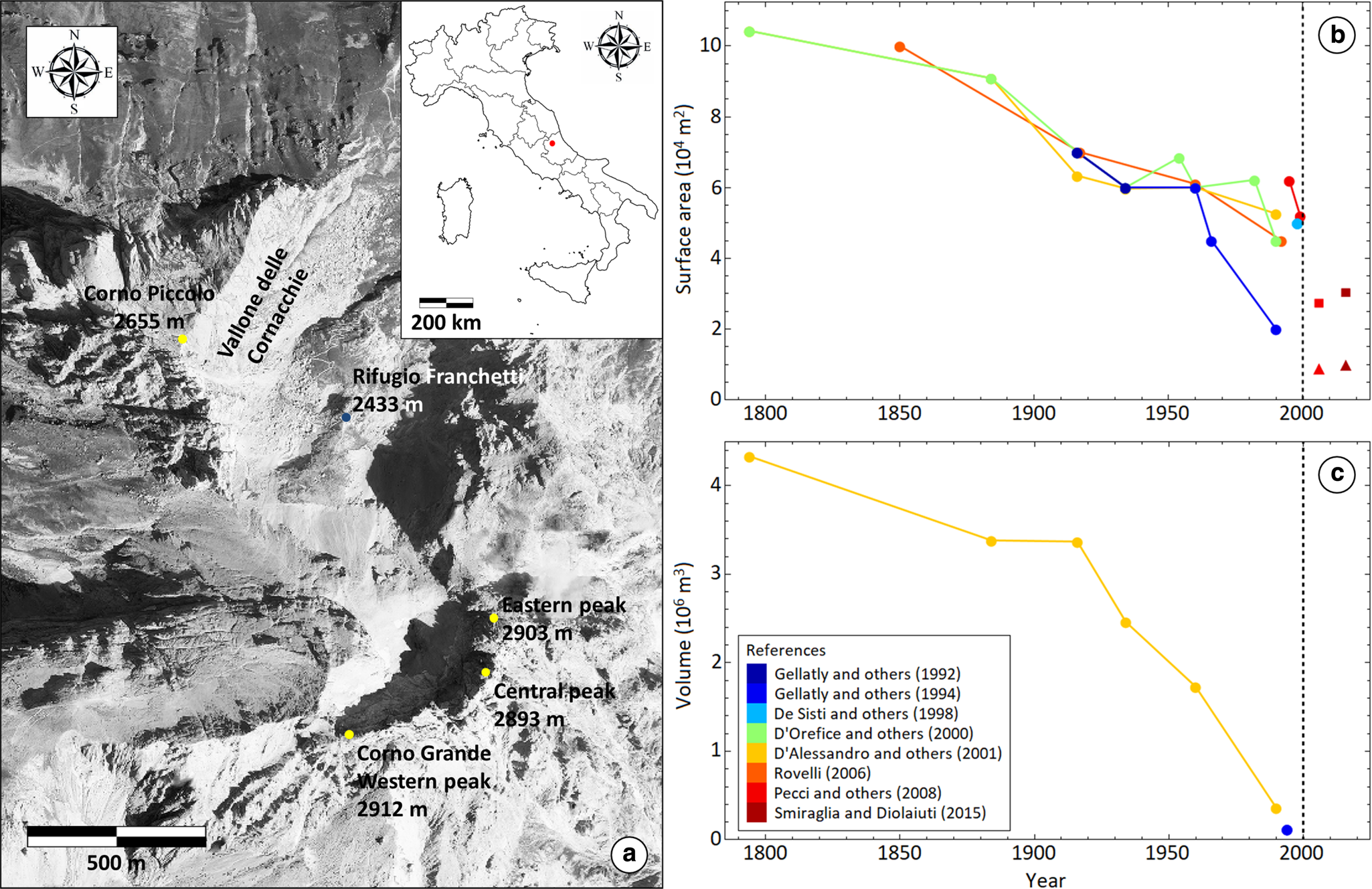
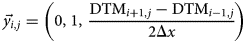
Figure 1. Location map and temporal evolution of the Calderone Glacier. The figure shows (a) the position (red dot) of the Gran Sasso d'Italia massif in central Italy, as well as an orthophoto of the Calderone Cirque and of the Vallone delle Cornacchie, with the positions of the Carlo Franchetti mountain lodge (blue dot) and of the main local mountain peaks (yellow dots) superimposed. The orthophoto is courtesy of the Abruzzo Region, and it is obtained from aerial digital photos taken in the 2018–2019 period. The figure also shows both the reconstructed and recorded temporal changes (colored dots) in the surface area (b) and the total volume (c) of the glacier, from the end of the LIA to the present, according to different authors. The vertical dashed line marks the year in which the glacier fragmented into the Lower (colored squares) and Upper (colored triangles) Glacierets. Note that the earliest value reported by Rovelli (Reference Rovelli2006) in (b) is simply defined as the maximum extent of the glacier in the XIX century, and therefore 1850 is used as a stand-in for the unspecified date.
The glaciers of the Gran Sasso d'Italia massif reached their maximum extensions during the Last Glacial Maximum (LGM; ~22 600 a BP), before starting to retreat ~21 000 a BP (Giraudi and Frezzotti, Reference Giraudi and Frezzotti1997). According to estimates, the seasonal snow limit averaged at 1750 m a.s.l. in the massifs of the Central Apennines during the LGM, reaching extremes of 1550 m a.s.l. in the western region and of 1990 m a.s.l. in the eastern region (Federici, Reference Federici1979; Pecci and D'Aquila, Reference Pecci and D'Aquila2011). The Calderone Glacier had five major expansion phases since the start of the Holocene epoch (~11 650 a BP), as observed from both local stratigraphic surveys and the carbon dating of soils interbedded with the deposited glacial till (Giraudi, Reference Giraudi2000, Reference Giraudi2005). Furthermore, the Holocene glaciation was limited to the Calderone Cirque and the upper section of the underlying Vallone delle Cornacchie (i.e. Deep Valley of the Crows; Fig. 1a), as inferred from the five known morainic systems (Giraudi, Reference Giraudi2000). Nevertheless, the significant steepness of the glacial valley could have either prevented the formation of other potential moraines, or significantly exacerbated their weathering (Giraudi, Reference Giraudi2000).
The two older moraines are located at 2350 m a.s.l. (i.e. the Cornacchie stage) and 2400 m a.s.l. (i.e. the Franchetti stage), respectively to the North-West and West of the nearby Carlo Franchetti mountain lodge (2433 m a.s.l.; Fig. 1a; Giraudi, Reference Giraudi2000); and they formed some time before 4000 a BP, during temporary reversals of a severe reduction phase (Giraudi, Reference Giraudi, Ehlers and Gibbard2004). In fact, the development of a soil layer within the Calderone Cirque between the second and third expansion phases, dated to 3890 ± 60 a BP, indicates a period of extreme reduction of the glacier, if not even its complete disappearance, starting from about 4300 a BP (Giraudi, Reference Giraudi2000, Reference Giraudi, Ehlers and Gibbard2004).
The three younger moraines (i.e. the Calderone 1, Calderone 2 and Calderone 3 stages) are found on the northern boundary of the Calderone Cirque (Giraudi, Reference Giraudi2000, Reference Giraudi2005). The Calderone 2 system constitutes the main part of the frontal moraine and overlays the Calderone 1 system, while the Calderone 3 system to the North-West is further divided into three smaller sections corresponding to three distinct sub-stages (Giraudi, Reference Giraudi2000, Reference Giraudi2005). In addition, parts of the Calderone 3 system lack a frontal section and their fallen debris can be found as far down as 2300 m a.s.l., due to a protruding glacier terminus during the Little Ice Age (LIA), when the Calderone Glacier reached its maximum extension of the last 4000 years (Giraudi, Reference Giraudi2000).
During the XIX century, the Calderone Glacier did not significantly change from its maximum extension in the LIA (Rovelli, Reference Rovelli2006); while a significant serac zone was still active until the end of the century, as inferred from the oldest available photographs from 1871 and 1887, and from morpho-chronological reconstructions (Pecci and D'Aquila, Reference Pecci and D'Aquila2011). Nevertheless, after the end of the LIA (~1850), the glacier entered a significant reduction phase that accelerated during the XX century, becoming even more pronounced during the last few decades and continues to the present day. This reduction phase is summarized in Figures 1b, c, as reported in the available literature (Gellatly and others, Reference Gellatly, Grove and Smiraglia1992, Reference Gellatly, Smiraglia, Grove and Latham1994; De Sisti and others, Reference De Sisti, Marino and Pecci1998; D'Orefice and others, Reference D'Orefice, Pecci, Smiraglia and Ventura2000; D'Alessandro and others, Reference D'Alessandro, D'Orefice, Pecci, Smiraglia, Ventura, Visconti, Beniston, Iannorelli and Barba2001; Rovelli, Reference Rovelli2006; Pecci and others, Reference Pecci, D'Agata and Smiraglia2008; Smiraglia and Diolaiuti, Reference Smiraglia and Diolaiuti2015) and inferred from reconstructed models, direct measurements, geodetic studies and geophysical surveys.
The historical models were based on detailed descriptions (Delfico, Reference Delfico1796; Marinelli and Ricci, Reference Marinelli and Ricci1916), paintings and drawings, accurate cartographic records dating between 1884 and 1990, as well as on-site pictures and aerial photos (D'Alessandro and others, Reference D'Alessandro, D'Orefice, Pecci, Smiraglia, Ventura, Visconti, Beniston, Iannorelli and Barba2001; Pecci, Reference Pecci, Visconti, Beniston, Iannorelli and Barba2001; Rovelli, Reference Rovelli2006). Between 1794 and 1990, D'Alessandro and others (Reference D'Alessandro, D'Orefice, Pecci, Smiraglia, Ventura, Visconti, Beniston, Iannorelli and Barba2001) show the glacier surface area and the total volume respectively decreasing by 49.6 and 91.7% (Figs. 1b, c). Similarly, D'Orefice and others (Reference D'Orefice, Pecci, Smiraglia and Ventura2000) show the surface area and the average ice thickness decreasing by more than 50% and more than 60% over the same period, respectively, with the reduction significantly accelerating in the second half of the XX century. Conversely, Pecci and others (Reference Pecci, D'Agata and Smiraglia2008) simulated a considerably more severe reduction (Table 1), by statistically correlating the 1995–2003 mass balances with meteorological data from Pietracamela (1000 m a.s.l., ~6 km North from the glacier). The variability in these models underlines the difficulty in accurately reconstructing past glacier evolutions in the absence of repeated and comprehensive field measurements.
Table 1. Historical and recent evolution of the Calderone glacial system between 1920 and 2006, as reported in Pecci and others (Reference Pecci, D'Agata and Smiraglia2008)
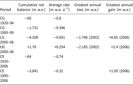
The table shows the cumulative net balance and the annual average for different periods, as well as a few notable annual values. After the fragmentation, the Lower Glacieret (LG) showed an almost consistent reduction, with only one other positive annual balance (i.e. +0.263 m w.e. in 2004), while the Upper Glacieret (UG) showed an almost consistent accumulation, with only one negative annual balance (Pecci and others, Reference Pecci, D'Agata and Smiraglia2008). After combining the estimates (CE) for the two glacierets with those for the Calderone Glacier (CG), the overall trend from 1995 to 2006 shows an almost consistent reduction, with only one other positive annual balance (i.e. +0.252 m w.e. in 2004; Pecci and others, Reference Pecci, D'Agata and Smiraglia2008)
1.2. Recent surveys and glacier fragmentation
Considering its declining trend, several multidisciplinary studies were conducted in the 1990s to assess the Calderone Glacier as a possible indicator of the effects of human activities, as well as of both regional and global climate changes (D'Alessandro and others, Reference D'Alessandro, D'Orefice, Pecci, Smiraglia, Ventura, Visconti, Beniston, Iannorelli and Barba2001; Pecci, Reference Pecci, Visconti, Beniston, Iannorelli and Barba2001). More recent preliminary surveys aimed at extracting, preserving and studying representative ice cores as part of the Ice Memory project, to reconstruct past trends in the global climate more accurately through geochemical analyses (Pavoni and others, Reference Pavoni2023). Since 1994, the mass balance of the Calderone Glacier has been measured annually using direct glaciological methods, with surveys respectively conducted at the end of the accumulation (i.e. late May – early June) and ablation (i.e. late September – early October) seasons (Pecci and others, Reference Pecci, D'Agata and Smiraglia2008). Further direct thickness measurements of the accumulated snow are usually performed at the beginning of the ablation season at representative sites, which include the areas in the vicinity of the inserted ablation stakes (Pecci and others, Reference Pecci, D'Agata and Smiraglia2008). Such measurements are generally coupled with the excavation of snow pits to locally evaluate the snow density in the shallower layers, and thus infer the corresponding WE (Pecci and others, Reference Pecci, D'Agata and Smiraglia2008).
The surface area covered during on-site surveys can sometimes be limited by the steepness of the local topography, as well as the significant risk of rockfalls from the elevated ridges enclosing the cirque (D'Orefice and others, Reference D'Orefice, Ledonne, Pecci, Smiraglia and Ventura1995, Reference D'Orefice, Pecci, Smiraglia and Ventura2000; Fiucci and others, Reference Fiucci, Gigante, Rossi, Smiraglia and Veggetti1997; De Sisti and others, Reference De Sisti, Marino and Pecci1998). In particular, the slope of the glacier surface has been estimated to range between 15° and 30° in the lower section, consistently remain ~30° in the middle section, and steadily increase from 30° to 40° in the upper section (Pecci and others, Reference Pecci, Visconti, Beniston, Iannorelli and Barba2001). In addition, direct measurements became increasingly more difficult over time due to the sustained accumulation of surface debris, in terms of both obtaining accurate readings from the ablation stakes and actually maintaining the network, especially in the lower section (Pecci and others, Reference Pecci, D'Agata and Smiraglia2008). On the other hand, several complementary geodetic observations have also been conducted over the years in the middle of both the summer and winter seasons, resulting in a comprehensive photographic archive (Pecci and others, Reference Pecci, D'Agata and Smiraglia2008). More than 200 images exist of the Calderone Glacier, just from the period between 1871 and 2005 (Rovelli, Reference Rovelli2006), which can thus be cross-referenced with the permanent local geographical features to obtain consistent and accurate geodetic models.
Furthermore, geophysical studies started being performed on the glacier, the earliest examples of which include GPR surveys performed in 1992, 1998 and 1999 (Fiucci and others, Reference Fiucci, Gigante, Rossi, Smiraglia and Veggetti1997; De Sisti and others, Reference De Sisti, Marino and Pecci1998; Pecci and others, Reference Pecci, Visconti, Beniston, Iannorelli and Barba2001). During the 1992 survey, the maximum ice thickness of the glacier was estimated at most equal to 26 m, under a debris cover that reached as much as 2 m in thickness in the lower section (Fiucci and others, Reference Fiucci, Gigante, Rossi, Smiraglia and Veggetti1997). The survey also highlighted a clear overdeepening, that is a deep depression in the underlying bedrock caused by previous rapid subglacial erosion (Fiucci and others, Reference Fiucci, Gigante, Rossi, Smiraglia and Veggetti1997). During the 1998 survey, the estimated thickness similarly ranged between 15 and 25 m in the lower section, and between 3 and 6 m in the middle section (De Sisti and others, Reference De Sisti, Marino and Pecci1998). During the 1999 GPR survey, the thickness of the lower section ranged between 3 and 27 m, averaging at 15 m, and the upper section reached a maximum thickness of 15 m, while the ice thickness in the middle section tapered down to nothing, thus dividing the glacier ice into two distinct patches (Pecci and others, Reference Pecci, Visconti, Beniston, Iannorelli and Barba2001). Overall, these GPR surveys highlighted a clear reduction in the ice thickness near the terminal moraine, as well as in the central part of the glacier, where rocky outcrops started to appear (Pecci and others, Reference Pecci, Visconti, Beniston, Iannorelli and Barba2001).
By the turn of the century, the glacier was almost completely concealed by a debris layer with a highly variable thickness (e.g. 0.001–1 m in the middle section), which made the identification of its boundaries more difficult in absence of thermal imagery (Shukla and others, Reference Shukla, Gupta and Arora2010; Gök and others, Reference Gök, Scherler and Anderson2023), but also helped maintain the buried ice in the lower section (De Sisti and others, Reference De Sisti, Marino and Pecci1998; D'Orefice and others, Reference D'Orefice, Pecci, Smiraglia and Ventura2000; Pecci and others, Reference Pecci, Visconti, Beniston, Iannorelli and Barba2001). Nevertheless, the Calderone Glacier eventually fragmented in the summer of 2000 into two smaller ice bodies, thus revealing the glacial sheepback (a.k.a., sheep rock or roche mountonnée) landform outcropping in-between them (Pecci and others, Reference Pecci, D'Agata and Smiraglia2008; Pecci and D'Aquila, Reference Pecci and D'Aquila2011). The upper and lower sections both lack any morphological evidence of glacier dynamics, with the last visible crevasses having been detected in the middle-to-lower section back in 1994, hence the current glacieret labels (Rovelli, Reference Rovelli2006; Smiraglia and Diolaiuti, Reference Smiraglia and Diolaiuti2015). The Lower Calderone Glacieret is located at the bottom of the enclosing cirque and is completely buried by a 0.05–1.5 m thick surface layer of rocky debris (Rovelli, Reference Rovelli2006); while the Upper Calderone Glacieret is located in the uppermost part of the cirque and consists mostly of ice and firn with little debris cover (Pecci and others, Reference Pecci, D'Agata and Smiraglia2008). These glacierets are believed to be the last two remaining perennial ice bodies in all of the Apennine Mountains, although a few small multi-year patches of snow can still be found within the mountain range (Smiraglia and Diolaiuti, Reference Smiraglia and Diolaiuti2015).
The more recent changes of the Calderone glacial system are summarized in Table 1, and combined with the reconstructed historical changes to highlight the evolution of its reduction phase (Pecci and others, Reference Pecci, D'Agata and Smiraglia2008). In particular, the more recent mass balance estimates show a noticeable decrease in the average reduction rate of the glacial system (Table 1), as a result of several factors that contribute to its endurance (Rovelli, Reference Rovelli2006), despite the overall reduction trend. In addition to the debris layer covering the Lower Glacieret and its elevated position, both the North-Eastern orientation of the Calderone Cirque and the significant elevation of the enclosing mountain ridges further reduce the exposure of the glacial system to solar radiation, while also leaving it open to the humid North–East winds from the Adriatic Sea (~45 km away; Fig. 1a). Subsequently, the abundant winter precipitations provide both direct and indirect accumulations, with the latter being caused by the frequent snow avalanches from the steep mountain sides (De Sisti and others, Reference De Sisti, Marino and Pecci1998; Pecci and others, Reference Pecci, Visconti, Beniston, Iannorelli and Barba2001; Pecci and D'Aquila, Reference Pecci and D'Aquila2011; Smiraglia and Diolaiuti, Reference Smiraglia and Diolaiuti2015).
In regard to the local climate, the Pietracamela weather station reported on average a slight decrease in the summer temperatures in the ten years after 1995, as well as a slight increase in the total winter snowfalls in the eight years after 1995, when compared to the preceding ten years (Pecci and others, Reference Pecci, D'Agata and Smiraglia2008). These trends could help explain the contemporary variability in the annual net balances, in particular the observed outliers of 2004 and 2006 (Table 1), which recorded significant net accumulations (Pecci and others, Reference Pecci, D'Agata and Smiraglia2008). In terms of their reported surface area, the Lower and Upper Glacierets slightly increased from 2.7 104 and 0.9 104 m2 in 2006 (Pecci and others, Reference Pecci, D'Agata and Smiraglia2008), to 3 104 and 104 m2 in 2011 (Smiraglia and Diolaiuti, Reference Smiraglia and Diolaiuti2015), respectively, although possible rounding-related differences should be taken into account. Other potentially distorting factors include the rocky debris cover causing an underestimation of the surface area, and the external residual snow causing an overestimation, with both effects being especially relevant during geodetic surveys. Smiraglia and Diolaiuti (Reference Smiraglia and Diolaiuti2015) further reported an average thinning rate for the two glacierets equal to about 1 m a−1.
2. Methods
2.1. GPR data acquisition
In this paper, we analyze three pseudo-3-D Common Offset (CO) GPR data sets that were acquired during the month of July in 2015, 2016 and 2019, over the Lower Calderone Glacieret (Fig. 2). The applied signal processing was limited to drift (a.k.a., time-zero or zero timing) correction, DC removal and a Butterworth band-pass filter. Even though migration is commonly applied to reconstruct the geometrically correct radar reflectivity distribution within the subsurface, especially regarding dipping reflectors (Jol, Reference Jol2009), this process was not used for the analysis. In particular, a correct migration analysis would (a) require an accurate EM velocity distribution as input, which is not yet known; (b) need equally spaced traces, which could necessitate the use of a rubber-band interpolation between dedicated marker points, in case of irregular spatial acquisition rates causing a stretching of the GPR image in-between such points (Jol, Reference Jol2009); and (c) potentially negatively impact the recovery of the ice-bedrock interface, which in most of the analyzed data sets is highlighted by interfering diffraction hyperbolas, rather than clear laterally coherent reflections.

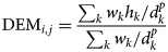
Figure 2. Trace positioning over the Lower Calderone Glacieret. The figure shows (a) a view of the Calderone Cirque from a photo taken by Dr Massimo Pecci on 15th September 2016; (b) the 3-D DTM of the Cirque obtained from the 2016 photogrammetric survey, with the contour lines plotted at 10 m elevation intervals, and the GPR survey lines of 2015 (black lines), 2016 (gray lines) and 2019 (light gray lines), superimposed; and (c) the normal versor (blue arrow) of a generic surface, resulting from the vector product of two gradient-based surface versors (black arrows), and used for the 3-D projection of the corresponding GPR trace. For reference, the positions (brown dots) of the nearby mountain peaks (Fig. 1a) are also highlighted in (b), with the mountain summit placed at the origin of both the easting and northing axes.
The three 2015 CO GPR profiles were acquired using a Zond-12e Radsys GPR system, equipped with 150 MHz air-coupled (hand-held) bistatic unshielded antennas (Monaco and Scozzafava, Reference Monaco and Scozzafava2017), with a transmitter–receiver offset of about 2.15 m and an average elevation above the ground-surface of ~20 cm. The same GPR system was later used to acquire the ten 2016 CO GPR profiles, two of which roughly coincide with the transversal profiles of the 2015 dataset (Fig. 2b). In absence of a GPS device during the data acquisition, the various GPR profiles were positioned using fixed reference points whose distance and elevation differences were measured with a Nikon Forestry Pro II Laser Rangefinder-Hypsometer (Monaco and Scozzafava, Reference Monaco and Scozzafava2017). In the presented analysis, the GPS coordinates of the western (42°28'10.596''N, 13°33'55.404''E) and eastern (42°28'19.812''N, 13°34'15.024''E) peaks of Mt. Corno Grande (Fig. 1a) were also used as a further constraint for the trace positioning (Fig. 2b).
The four 2019 CO GPR profiles were instead acquired using a PulseEkko Pro GPR system equipped with 250 MHz ground-coupled bistatic Sensors & Software Inc. shielded antennas, with a transmitter-receiver offset equal to 27.94 cm. The various GPR profiles were positioned using specific markers that were accurately recorded at regular intervals along the corresponding survey lines.
A photogrammetric survey (Pecci and others, Reference Pecci, Cappelletti, Esposito, D'Aquila and Caira2017) was also carried out on 15th September 2016 (i.e. at the end of the ablation season), from which a Digital Terrain Model (DTM) was constructed (Fig. 2b). Considering the initial approximate 13 × 13 cm resolution, the Point Sampling Tool plug-in of the QGIS open source software was used to discretize the entire surface of the Calderone cirque into a 1 × 1 m grid for the analysis. The obtained DTM was then used as a reference surface to study the glacieret volume, by comparing it with the basal interfaces constructed over the same grid from each GPR survey. For georeferencing purposes, a few GPS measurements were further acquired at specific reference points on the glacieret surface, such as large boulders (Pecci and others, Reference Pecci, Cappelletti, Esposito, D'Aquila and Caira2017).
It is important to point out that the use of the same 2016 DTM in all three cases may introduce an additional uncertainty factor, due to potentially significant variations in the surface topography (either local or global) with respect to both 2015 and 2019, that could be caused by changes in both the glacieret volume and the debris cover. Nevertheless, the use of a reference DTM is necessary for a more accurate estimation of the glacieret volume, in absence of a specific DTM for each year, especially considering the highly variable topography of the surveyed area (Pecci and others, Reference Pecci, Visconti, Beniston, Iannorelli and Barba2001).
2.2. Time-to-depth conversion
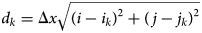
The basal interface of the Lower Glacieret was recovered using an automated reflection strength tracking algorithm designed to track the recorded reflections accurately and objectively along the various GPR profiles (Dossi and others, Reference Dossi2022a). As an example, the horizons marking the main reflections within the longitudinal profiles of the various GPR surveys are highlighted in Figure 3a, showing no significant internal stratigraphy. This lack of internal reflections, combined with the significant presence of surface debris, prevents the implementation of an amplitude inversion algorithm designed to recover the subsurface EM velocity distribution from the identified reflection amplitudes and arrival times (Forte and others, Reference Forte, Dossi, Pipan and Colucci2014; Dossi and others, Reference Dossi, Forte, Pipan and Colucci2018).
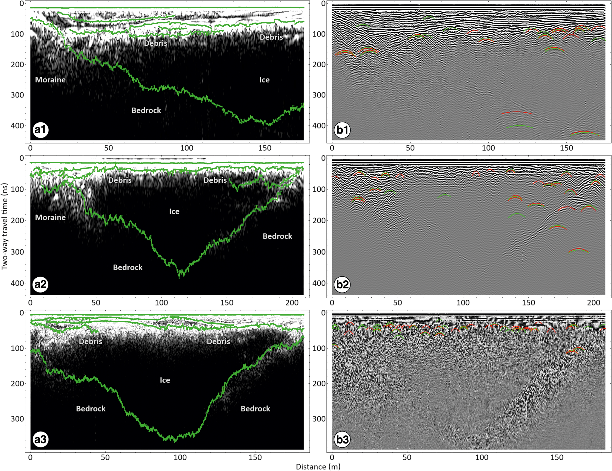
Figure 3. Auto-tracking results for the 2015 (first row), 2016 (second row) and 2019 (third row) longitudinal GPR profiles. In each row, the figure shows (a) the auto-tracked horizons (green lines) marking the main recorded reflections, superimposed to the reflection strength profile; and (b) the auto-picked diffraction hyperbolas, superimposed to the corresponding signal amplitude profile, with positive amplitudes marked in green and negative amplitudes marked in red.
As an alternative, the hyperbolic diffractions within the various GPR profiles were recovered using an automated diffraction picking algorithm designed to detect subsurface scatterers objectively, track the diffraction phases originating from them accurately, and recover the average subsurface EM velocity above each scatterer, among other possible analyses (Dossi and others, Reference Dossi2022b, Reference Dossi2024). The hyperbolas constructed from the aforementioned longitudinal profiles are shown in Figure 3b, and they accurately mark most of the recorded diffractions. As it can be noticed from the results, however, the number of clear undistorted diffractions is limited to a few dozens, which makes the resulting EM velocity model more susceptible to the presence of false positives. In fact, to avoid a significant number of noise-related false negatives, we intentionally did not apply the automated grouping analysis in Figure 3b, which disregards isolated false positives by requiring each constructed hyperbola to have at least one other hyperbola of opposite polarity marking another phase of the same diffraction event (Dossi and others, Reference Dossi2022b, Reference Dossi2024).
The shape of the available diffractions can also be affected by (a) the possibly erroneous positioning of the individual GPR traces; (b) the possible presence of out-of-plane diffractions, whose in-plane projections would be placed at the wrong depths; and (c) substantial signal interference, random noise and clutters (Dossi and others, Reference Dossi2022b, Reference Dossi2024). More importantly, the identified diffractions in Figure 3b are mostly concentrated in the shallower section of the glacieret, as in all the other GPR profiles, therefore no significant information regarding the EM velocity within the deeper region can be recovered with this method. As a result of all these issues, it was determined that a statistically sound EM velocity distribution within the Lower Calderone Glacieret could not be recovered from the available GPR data.
For the time-to-depth conversion, we therefore used a reference EM velocity equal to 0.168 m ns−1, corresponding to pure ice (Looyenga, Reference Looyenga1965), and an associated uncertainty of 10%. The possible glacial systems covered by the considered EM velocities thus range between compact firn at the higher end (Looyenga, Reference Looyenga1965; Robin, Reference Robin1975; Kovacs and others, Reference Kovacs, Gow and Morey1995), and ice containing liquid water for about 2.5–3% of the total volume at the lower end, as estimated from volumetric mixing models (Birchak and others, Reference Birchak, Gardner, Hipp and Victor1974). The selected uncertainty can also be assumed to cover the irregular 0.05–1.5 m thick surface debris layer (Rovelli, Reference Rovelli2006), for which the effect on the total cumulative EM velocity is difficult to be determined locally, with the EM velocity for limestone being equal to 0.12 m ns−1 (Davis and Annan, Reference Davis and Annan1989).
In any case, the debris cover will have an overall negligible effect in the calculation of the total thickness, particularly in the deeper areas of the glacieret, when compared to other possible sources of uncertainty, which include (a) possible local deviations from the globally-applied data acquisition and signal processing parameters, such as the utilized trace interval and drift correction; (b) the automatically picked arrival times of the basal reflections, which correspond to the individual peaks of the phase-independent reflection strength in each GPR trace (Fig. 3a; Dossi and others, Reference Dossi2022a), and can be negatively affected by significant noise and interference; (c) the avoidance of migration processes in the applied signal processing, which require accurate EM velocity distributions as input to move dipping reflectors to their correct positions within GPR profiles (Jol, Reference Jol2009); and (d) the normal projections of the estimated thicknesses onto the glacieret surface (Fig. 2c; discussed in the following section), which can be affected by local outliers in the DTM (Fig. 2b), as well as erroneous trace positioning.
2.3. Digital elevation model of the glacieret base
After the time-to-depth conversion, the tracked basal reflections were projected onto the vertical axes of the individual GPR traces, which were locally estimated from the surrounding topography. In particular, the versor $\hat{n}_{i,j}$ normal to the DTM at a given trace position is calculated through the vector product of the two vectors $\vec{x}_{i,j}$
 and $\vec{y}_{i,j}$
 (Fig. 2c), which are obtained from the respective components of the local gradient vector of the DTM:

with
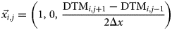
where (j, i) is the closest gridpoint to the considered GPR trace position, and Δx is the space interval (i.e. 1 m) used to discretize both the easting and northing positions within the grid. To avoid possible outliers in the calculated normal versors, potentially caused by either isolated artifacts or peculiar small-scale changes in the topography, the gradient vector in each position (whose components are used in Eqns. (2), (3)) was substituted with an average of the local gradient vectors of the DTM (i.e. within a 10 m radius).
After positioning the basal lines within the 3-D model, these were combined with the contour lines of the DTM outside of the glacieret surface (Fig. 2b), to construct a digital elevation model (DEM) of the glacieret base. More specifically, the surrounding contour lines were marked from the DTM at 5 m elevation intervals and used as a boundary condition during the interpolation process, while the extent of the debris-covered glacieret was roughly inferred from the thicknesses estimated at the edges of the various GPR surveys, as well as from the available photographic data. Furthermore, to avoid data redundancy and reduce computational costs, given the high linear density of GPR traces when compared to the grid resolution, the basal lines were re-sampled at 0.5 m elevation intervals using a simple 3-D linear interpolation between adjacent GPR traces.
The elevation of the basal DEM at the various grid positions was calculated using the adjusted IDW spatial interpolation method presented by Li and others (Reference Li, Wang, Ma and Wu2018). Considering N H elevation points that belong to either the basal or contour lines, the elevations h k of these points, and their horizontal distances d k from the interpolation point located at the (j, i) grid position, the elevation of the DEM at such position is given by the following weighted average (Achilleos, Reference Achilleos2011; Rui and others, Reference Rui, Yu, Lu, Ashraf and Song2016; Li and others, Reference Li, Wang, Ma and Wu2018):
with


where (j k, i k) and w k are respectively the position and adjusting parameter of the k-th point of the set; and the exponent p defines the type of interpolation used, namely (assuming all w k being equal to 1) either a moving average (i.e. p = 0), a linear interpolation (i.e. p = 1), or a weighted moving average (i.e. p > 1). In fact, the higher the value of p is, the smoother the resulting DEM surface becomes (Li and others, Reference Li, Wang, Ma and Wu2018).
For the construction of the set of N H elevation points, we used linear segments branching out of the considered (j, i) grid position at regular angular intervals Δϕ (e.g. 15°), to mark the crossed elevation points along the N L (e.g. 2) closest basal or contour lines to be reached by the segment each time. In addition, after crossing the closest line, each segment is iteratively rotated counterclockwise by Δϕ/N L for each of the remaining N L − 1 lines to be crossed, to avoid the adjusting parameter of the next crossing point to be identically null due to the latter being directly behind the previous point. In particular, the adjusting parameters w k, which may not be commonly applied in IDW interpolations (Achilleos, Reference Achilleos2011), are used in Eqn. (4) to reduce the influence of the elevation points further away from the analyzed interpolation point, due to the presence of closer elevation points in-between (Li and others, Reference Li, Wang, Ma and Wu2018).
In the calculation of the adjusting parameters, the marked N H elevation points are re-arranged by increasing values of d k (Eqn. (5)). As each point effectively casts a shadow onto the points further away, the resulting cumulative effect onto the k-th elevation point, caused by some of the k − 1 closer points, is based on the relative angular positions of the former with respect to each one of the latter. In particular, the adjusting parameter for the k-th elevation point is given by (Li and others, Reference Li, Wang, Ma and Wu2018):
with
where θ k,m is the angle formed by the segment connecting the compared k-th and m-th elevation points, and the segment connecting the interpolation point with the midpoint of the first segment; α k,m is the angle formed by such elevation points, with the vertex placed on the interpolation point; α max is the maximum angle for α k,m, above which the closer m-th point does not cast a shadow onto the k-th point further away; and max[…] is an operator that provides the maximum value among those listed within its argument.
As it can be noticed from Eqn. (7), when the angle α k,m is equal or greater than α max, the angle θ k,m is automatically set equal to π/2, which in turn sets the corresponding factor in Eqn. (6) equal to 1, thus canceling out the influence of the latter in the calculation of w k. Therefore, the elevation points that have no other point located between them and the interpolation point, will have an uninfluential adjusting parameter w k (i.e. equal to 1). Notice that the product in Eqn. (6) only considers the elevation points that are closer than the k-th point to the interpolation point, while the first elevation point of the set (i.e. k = 1) has a value of w k equal to one (Eqn. (6)), since by construction it has no other elevation point in-between.
Given the potentially large number N H of elevation points involved in the IDW interpolation at each grid position, the angular step Δϕ is used as a minimum value for α max in Eqn. (8), to prevent the latter from becoming uselessly small in Eqn. (7). In addition, the set number N L of the closest contour or basal lines involved in the analysis is added as a factor in Eqn. (8), as opposed to the formula used in Li and others (Reference Li, Wang, Ma and Wu2018), since the analyzed elevation points are not randomly distributed, but rather selected through a geometrically determined process. The added factor thus further prevents the resulting angle from becoming too small, and roughly defines the average angular interval within each of the N L constructed arrays.
2.4. Potential DEM artifacts
Common IDW interpolations generally perform better when the sampled elevation points are regularly distributed, while possible artifacts include the topographic island effect, by which both hills and basins are turned flat within the innermost circles in topographic maps; and the bull's eye effect, by which isolated DEM peaks stick out at the various elevation positions (Achilleos, Reference Achilleos2011; Li and others, Reference Li, Wang, Ma and Wu2018).
The latter effect is caused by the significantly smaller distance d k of a given elevation point when the IDW interpolation is performed in its neighborhood, which disproportionally increases the weight of such point by almost turning it into a singularity (Eqn. (4)). The added adjusting parameters w k (Eqn. (6)) counteract these artifacts by reducing the influence of the points further away while increasing the relative weight of the closer ones (Fig. 4), which likely have elevations similar to the considered point, although the distorting effect may not completely disappear (Li and others, Reference Li, Wang, Ma and Wu2018). For instance, the alternation between the constructed basal and contour lines and the void areas in-between caused a slight stair-stepping effect (a.k.a., staircase effect) that rendered those lines noticeable in the resulting DEMs of the bedrock.
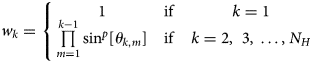
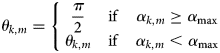
Figure 4. Exemplary shadow effect between two elevation points, used to prevent bull's eye artifacts during the IDW spatial interpolation. The figure shows (a) the interpolation point (blue dot), the first elevation point (gray dot), and the different (numbered) positions of the second point (brown dots), with the segments (dashed lines) separately connecting the interpolation point with the elevation points in the various cases, and with the angle α 2,1 (Eqn. (8)) at the first position highlighted (yellow sector); and (b) the same geometry as in (a), with one set of segments (solid lines) connecting the two elevation points (gray and brown dots) in the different cases, and the other (dashed lines) connecting the interpolation point (blue dot) to the midpoints (red dots) of the former in said cases, and with the angle θ 2,1 (Eqns. (7), (9)) at the first position highlighted (yellow sector). The figure also shows (c) the angles α 2,1 (blue dots) and θ 2,1 (red dots) formed in the various cases by the segments in (a) and (b), as well as the maximum value α max (dashed line), set equal to 15° in this example; and (d) the elevation (blue dots) extrapolated in the interpolation point in the different geometries, compared to the constant elevations for the first (gray line) and second (brown line) points, chosen as an example.
As an example of the shadow effect between two elevation points in the adjusted IDW spatial interpolation, Figure 4 shows the effect of the adjusting parameter w 2 of the second point, for 11 different positions with respect to the (closer) first one. In the considered case, Eqn. (4) is simplified into the following equation:

The effects of the shadow cast by the first elevation point onto the second one are visible in Figure 4d at the positions 3–8 of the second point. Most notably, an abrupt change in the interpolated elevation can be noticed between the positions 8 and 9 (Fig. 4d), caused by the angle α 2,1 surpassing the threshold α max (Fig. 4c), while the asymmetry in the graphs is mainly caused by the increasing distance d 2 (Fig. 4a).
3. Results
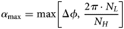
The construction process of the basal DEMs of the Lower Calderone Glacieret is presented in Figure 5, for the different GPR surveys. As it can be noticed, the utilized basal and contour lines tend to not be as regularly distributed along the analyzed grid as they would be expected in the ideal case (Li and others, Reference Li, Wang, Ma and Wu2018). This is most prominently the case for the 2015 (Fig. 5a-1) and 2019 (Fig. 5a-3) data, where large gaps can be observed between the basal and contour lines, in the areas not covered by the GPR surveys. Irregular distributions can also be observed in the 2016 dataset (Fig. 5a-2), namely at the abrupt transitions between the transversal basal lines and the longitudinally oriented contour lines, as well as at the relatively smaller gaps in the steeper southern section of the glacieret. The artifacts originating from such data arrays can be noticed in the constructed basal DEMs (Fig. 5b), although they ultimately affect the resulting 3-D models at very different degrees.

Figure 5. Construction of the basal DEMs of the Lower Calderone Glacieret from the 2015 (first column), 2016 (second column) and 2019 (third column) GPR surveys. In each column, the figure shows (a) the utilized basal and contour lines (blue pixels), and the horizontal distances (dashed lines) between the elevation (brown dots) and interpolation (blue dots) points used in the calculation of the DEM at eight exemplary locations (Eqn. (4)); and (b) the contour plot of the resulting DEM, with superimposed the basal lines (black dots) obtained from the GPR profiles and re-sampled at 0.5 m elevation intervals. For visual clarity, the blue dots in (b) highlight bed elevations equal to the corresponding plotted contour lines, which mark 5 m elevation intervals, similarly to the topographic contour lines in (a).
In the 2015 DEM, the IDW interpolation replaced the large gaps generally with inward bumps (Fig. 5b-1), as opposed to the expected basin, mainly due to the larger influence of the elevated and relatively closer contour lines (Fig. 5a-1). Similar deformations can also be noticed on the left side of the 2019 DEM, while on the right side the reconstructed interface shows an unrealistically smooth surface in the transition between the contour and basal lines (Fig. 5b-3). Apart from a preemptively higher data density over the surveyed area, a theoretical post-acquisition solution for these kinds of artifacts could be an increase in the number of elevation points marked along the basal lines for the IDW interpolation, with respect to those in the contour lines, albeit with a subsequent increase in the computational cost. Alternatively, the weights of the basal lines could be purposefully increased in the calculation of the DEM, either subjectively or based on a specified radiation pattern. In the case of the 2015 and 2019 data sets, we attempted to obtain more realistic basal DEMs by applying an elliptical IDW method (Merwade and others, Reference Merwade, Maidment and Goff2006), which would have better accounted for the directional morphology of the glacieret base. In particular, at each interpolation point (e.g. blue dots in Fig. 5a) the weights of the various elevation points used in the calculation (i.e. brown dots in Fig. 5a) were modified by projecting the corresponding distances (Eqn. (5)) onto ellipsoidal surfaces that were iteratively fitted to the different sets of elevation points (Ying and others, Reference Ying2012). However, these attempts were ultimately abandoned, since the resulting changes were deemed to be negligible within the gaps, while also being excessively distorting in the more densely sampled areas.
The 2016 DEM can be considered acceptable for further analyses of the surface area and volume of the Lower Calderone Glacieret, although some tongue-shaped artifacts can still be noticed, especially on the left side of the survey area (Fig. 5b-2). These can be attributed to both the aforementioned abrupt transitions between the basal and contour lines, and possible trace positioning errors that, for instance, could cause a given transversal GPR profile to be locally shifted with respect to the two adjacent ones. Nevertheless, useful information can still be recovered from the reconstructed basal topography model (Fig. 6a), which also includes the upper and lower uncertainty DEMs (Fig. 6b). The latter were constructed by applying the same IDW interpolation process used for the reference basal DEM (Fig. 5a-2), however the EM velocities used for the time-to-depth conversion (which defines the basal lines) are respectively equal to the lower and upper ends of the previously discussed ±10% range.
Figure 6. Thickness of the Lower Calderone Glacieret, as inferred from the various models. The figure shows (a) the difference in elevation between the DTM (Fig. 2b) of the glacieret surface and the 2016 DEM (Fig. 5b-2) of the glacieret base, with the obtained surface boundary (red line) following the null-thickness contour line; and (b) a cross section of the 2016 DTM and DEM (sienna tones), that includes the upper and lower DEMs (silver tones), which highlight the uncertainty of the reconstructed basal interface. For completeness, the figure also shows the difference between the DTM and the reconstructed 2015 (c) and 2019 (d) basal DEMs (Figs. 5b-1, b-3), in which artificial negative thicknesses can be observed in the large areas not covered by the respective GPR surveys.
The surface area of the glacieret was obtained from the null-thickness contour line (Fig. 6a) of the difference between the surface DTM (Fig. 2b) and the basal 2016 DEM (Fig. 5b-2). The identified surface area is equal to 2.37 104 m2 on the horizontal plane, while it is equal to 2.71 104 m2 when the local topography is taken into account, with the glacieret surface being approximated as planar between each triplet of adjacent points forming a right triangle within the grid (Fig. 2c). These approximated estimates are comparable with both the 2.7 104 m2 estimated by Pecci and others (Reference Pecci, D'Agata and Smiraglia2008) for 2006, and the possibly rounded-up 3 104 m2 reported by Smiraglia and Diolaiuti (Reference Smiraglia and Diolaiuti2015) for 2011 (Fig. 1b). In terms of volume estimates, the average vertical thickness (i.e. DTM-DEM difference) calculated within the horizontal area is equal to 13.3 ± 1.5 m, where the associated uncertainty is given by the average differences between the reference basal DEM and the upper and lower DEMs (Fig. 6b). Consequently, the total volume of the Lower Calderone Glacieret in 2016 is calculated as 3.15 105 ± 0.35 105 m3, which is comparable with the 3.61 105 m3 estimated by D'Alessandro and others (Reference D'Alessandro, D'Orefice, Pecci, Smiraglia, Ventura, Visconti, Beniston, Iannorelli and Barba2001) for 1990 (Fig. 1c), and almost three times the 1.2 105 m3 roughly estimated by Gellatly and others (Reference Gellatly, Smiraglia, Grove and Latham1994). Notice that both historical estimates include the upper section of the then still whole Calderone Glacier, while the high variability in the estimated glacieret volumes highlights the difficulty in accurately reconstructing its basal interface. In fact, considering the significantly reduced size of the glacieret, the irregularity of the basal topography constitutes an ever more influential uncertainty factor in the estimation of the total glacieret volume.
This is particularly evident when considering the volume-area scaling (VAS) empirical relations, which are widely applied in glacier inventories and water resource estimations, and are based on data from large populations of studied glaciers (Bahr and others, Reference Bahr, Pfeffer and Kaser2015; Colucci and Žebre, Reference Colucci and Žebre2016). As an example, two functions that have been used to estimate the volume of glaciers and glacierets from their surface areas, are given by (Bahr and others, Reference Bahr, Pfeffer and Kaser2015; Colucci and Žebre, Reference Colucci and Žebre2016):


where V and S are respectively the volume (in km3) and the surface area (in km2) of the considered glacial bodies.
Since volume-area relationships might fail for glacier sizes that fall outside the range of the observed data (Bahr and others, Reference Bahr, Pfeffer and Kaser2015), Eqn. (11) was proposed by Colucci and Žebre (Reference Colucci and Žebre2016) specifically for small and very small glaciers and glacierets, down to ice patches covering just 104 m2, in order to reconstruct the evolution of glaciers in the southeastern Alps during the Late Holocene. Although the sizes of the Upper and Lower Calderone Glacierets (Fig. 1b) fall within the acceptable range for Eqn. (11), as this relation defines an average trend within the considered statistical population, the accuracy of the resulting estimates might not be considered acceptable for further quantitative analyses (e.g. WE estimation). For instance, while the estimated 2.71 104 m2 topographic surface area and the 3.15 105 ± 0.35 105 m3 total glacieret volume are comparable with the fitted glaciological data (Colucci and Žebre, Reference Colucci and Žebre2016), the Lower Glacieret volume obtained from Eqn. (11) would be equal to 5.17 105 m3, which is about 64.1% higher than the estimated 3.15 105 m3 mean volume.
4. Discussion
Irrespective of the morphology and surface area, the dependence of the reconstructed DEM on the particular spatial interpolation method used is observed to decrease with increasing elevation data density (Chaplot and others, Reference Chaplot2006). More specifically, Chaplot and others (Reference Chaplot2006) report few differences between the techniques studied, provided that the sampling density was high, simply due to the decrease of the average distance between the known values. Similarly, Aguilar and others (Reference Aguilar, Agüera, Aguilar and Carvajal2005) concluded that the factor that has the greatest influence on the quality of the surface interpolated from scattered data was the landscape morphology, followed by the sampling density, and then by the applied interpolation method.
Regarding the reconstructed DEMs, the difficulty in obtaining accurate volume estimates can also be noticed when observing the negative thicknesses obtained in areas not covered by their respective GPR surveys. In the 2016 model, these artifacts are located outside of the identified glacieret boundaries (Figs. 6a, b), due to the basal DEM being slightly higher than the surface DTM in some areas; and they can be expected for the surrounding topography, where the interpolated DEM and the recorded DTM are supposed to coincide. On the other hand, these artifacts have a much more substantial presence in the 2015 (Fig. 6c) and 2019 (Fig. 6d) models, even within the 2016 boundaries, due to the more limited areas covered by the GPR profiles. In particular, the straightforward IDW interpolation connecting the basal and contour lines over the aforementioned gaps (Figs. 5a-1, a-3) caused the resulting DEMs (Figs. 5b-1, b-3) to have an elevation that is significantly higher than the DTM of the glacieret surface. Therefore, it is ultimately not possible to estimate the volume of the Lower Calderone Glacieret accurately and objectively from the 2015 and 2019 models, which would have allowed to examine its recent evolution together with the 2016 model. Another possible method to obtain these volume estimates would have been to compare the basal DEM from 2016 with surface DTM from the other years, however such data are not available for the presented analysis.
Nevertheless, it is still possible to compare the thicknesses of the different models along their respective basal lines, with the resulting average values for the 2015, 2016 and 2019 surveys being respectively equal to 16.1, 14.6 and 15.4 m. As it can be noticed, the 2016 average thickness calculated along the basal lines is just within the upper limit of the uncertainty interval of the value obtained over the entire surface of the glacieret model (i.e. 13.3 ± 1.5 m), which highlights the importance of a 3-D analysis for accurate volume estimates, compared to a 2-D one. In any case, as the 2016 3-D glacieret model is the only one available, a more direct comparison between the surveys would theoretically be to analyze the thicknesses along the same paths within such model, which results in the aforementioned average values being respectively equal to 12.5, 14.6 and 15.3 m. However, this comparison is not valid due to the previously discussed trace positioning issues, which can lead to significant discrepancies within those areas that are not covered by all surveys, since such areas rely more heavily on the accuracy of the IDW interpolation. An additional uncertainty factor is the use of the same 2016 DTM in all three cases (Fig. 2b), with DTMs from the other years not being available. Therefore, the analysis does not take into account possible temporal changes in the surface topography, whether locally or globally, with respect to both 2015 and 2019.
Nevertheless, the most noticeable differences in the thickness of the different models along the basal lines can be observed at the edges of such lines (Fig. 6). In particular, the large differences between the 2016 and 2019 models are mainly responsible for the potentially misleading increase in the calculated average thickness from 14.6 to 15.4 m. More specifically, the higher thicknesses obtained at the southern end of the 2019 survey (Fig. 6d) would indicate a deeper basal interface with respect to the 2016 model (Fig. 6a) over the same area. Notwithstanding possible temporal changes in the local topography, these discrepancies can be attributed to a local lack of data within the 2016 dataset, thus highlighting another uncertainty factor that can be expected from spatially limited GPR surveys.
5. Conclusion
We presented a quantitative GPR analysis in which we constructed and compared the basal DEMs of the Lower Calderone Glacieret for 2015, 2016 and 2019; while also discussing both the advantages and limitations of the implemented procedure. We highlighted the need for GPR surveys that cover the entire surface of a glacier at regular intervals, as well as for accurate internal EM velocity distributions for the time-to-depth conversion, to estimate of the total volume as accurately as possible. This issue is especially relevant for small glaciers and glacierets, in which peculiar topographical anomalies constitute a significant uncertainty factor compared to the smaller sizes of these ice bodies.
In the case of the Lower Calderone Glacieret, the lack of a clearly identifiable internal stratigraphy, combined with the significant surface debris cover, and the localization of the small number of usable undistorted diffractions within the shallower sections, prevented the reconstruction of the internal EM velocity distribution by means of either amplitude inversion or diffraction analysis. We therefore used a reference EM velocity equal to 0.168 m ns−1, with an associated uncertainty of ±10%, for the time-to-depth conversion. In regard to the recent temporal changes, the low data densities of the 2015 and 2019 GPR surveys ultimately prevented a direct comparison between the various glacieret models in terms of the resulting volumes. However, a 2-D analysis of the individual GPR profiles still suggests a general decrease in the average glacieret thickness over time.
The reconstructed glacieret model for 2016 allowed us to calculate a topographic surface area of 2.71 104 m2 and a total volume of 3.15 105 ± 0.35 105 m3. Both values are consistent with the more recent estimates from literature, although the logistical difficulties in surveying the steeper upper section of the glacieret could have caused a slight underestimation. In conclusion, considering the challenging terrain, the presented case study demonstrated the advantages of GPR surveys with respect to more traditional glacier monitoring techniques. In particular, its ability to probe the entire volume of the debris-covered glacieret at high data densities significantly improved the validity of the reconstructed 3-D model.
Acknowledgements
The study presented in this paper was carried out within the framework of the project ‘Misure delle proprietà fisiche, dello spessore dei ghiacciai e del manto nevoso in Appennino centrale e loro evoluzione temporale’, funded by the Presidency of the Council of Ministers - Department for Regional Affairs and Autonomies (Dipartimento per gli Affari Regionali e le Autonomie della Presidenza del Consiglio dei Ministri). We gratefully acknowledge the Region of Abruzzo for allowing the publication of their orthophoto under the terms of the Image Use Policy of the ‘Geoportale della Regione Abruzzo’ online catalog, which grants a CC BY-NC 3.0 License for the utilized image. We also wish to thank the Meteorological Association ‘AQ Caput Frigoris’, as well as Paolo Boccabella, Tiziano Caira, Domenico Cimini, Pinuccio D'Aquila, Thomas Di Fiore, Giulio Esposito, Alessandro Ferrante, Cristiano Iurisci, Giampiero Manzo, Manuel Montini, Mattia Pecci, Edoardo Raparelli, Valerio Sorani, Paolo Tuccella and Francesco Vaccaro, for their technical and logistical support. Special thanks to the late prof. Frank Silvio Marzano for his irreplaceable contribution to the promotion of new scientific efforts to study the natural processes occurring on the summit of the Gran Sasso d'Italia massif, which led in large part to the presented work.


 Open access