





Impact Statement
Robot swarms are suitable for a variety of tasks, many of which entail the swarm maintaining a certain spatial configuration, called formation. However, the application of robot swarms is subject to safety and reliability concerns, for instance, when operating near humans or handling sensitive information. Different issues, ranging from hardware errors to cyber-attacks, can manifest as anomalies in the physical motions of robots. This work investigates a data-driven method for detecting anomalous motion behavior in robot formations. The method is trained to learn the expected, normal behavior of robots, while not knowing any specifics of anomalous motions. When applying the anomaly-detection method to unknown instances of swarm formation tasks, anomalies can be identified as deviations from normal robot behavior.
1. Introduction
Autonomous multiagent systems have gained a lot of attention in many research areas over the recent years, with the use of robot swarms in particular having been studied for various problem settings like environmental monitoring and exploration (Chen et al., Reference Chen, He, Lennox, Arvin and Atapour-Abarghouei2025) or agricultural tasks (Albani et al., Reference Albani, IJsselmuiden, Haken and Trianni2017). Within these use cases, a common task of swarms is to maintain a desired spatial configuration, also called formation control (Ahn, Reference Ahn2020). As a subtopic of swarm robotics, formation control is used, for instance, for transporting objects (Ebel, Reference Ebel2021; Rosenfelder et al. Reference Rosenfelder, Ebel and Eberhard2024), platoon driving of autonomous vehicles (Balch and Arkin, Reference Balch and Arkin1998), and formation flight of drones (Saska et al., Reference Saska, Hert, Baca, Kratky and Nascimento2020). Controlling the movement of a robot formation can be a challenging task, as individual robot motions possibly exert a strong influence on the actions of other formation members. Therefore, formation tasks generally presuppose the correct behavior of all agents (Olfati-Saber et al., Reference Olfati-Saber, Fax and Murray2007).
While the use of robot swarms appears promising in terms of increasing effectiveness as well as efficiency, employing robot swarms in real-world scenarios is still uncommon (Schranz et al., Reference Schranz, Umlauft, Sende and Elmenreich2020). Networked robotic systems are sensitive to malfunctions and malicious attacks regarding both the communication and the physical actions of individual agents (Nguyen et al., Reference Nguyen, Ngo, Tuan, Phan and Tan2025), and major concerns regarding safety and reliability are a limiting factor for the large-scale adoption of swarm robotics in many application fields (Schranz et al., Reference Schranz, Umlauft, Sende and Elmenreich2020). For the specific setting of robot formations, antagonistic formation members can pose a serious security threat depending on the formation task, for example, when transporting heavy objects in the presence of human coworkers. While the literature on detecting antagonistic attacks in robot swarms is largely focused on malicious network activities and cybersecurity (Basan et al., Reference Basan, Basan and Nekrasov2019; Deng et al., Reference Deng, Zhou, Xu, Zhang and Liu2021), this work will specifically investigate anomalous or antagonistic behavior that manifests in the physical motions of a robot. Previous work on the detection of physically anomalous behavior of agents assigned to a formation task include an observer-based approach proposed in Zhao and Yu (Reference Zhao and Yu2023) as well as a supervised learning approach investigated in Wang et al. (Reference Wang, Shang and Sun2011). However, the neural network utilized in Wang et al. (Reference Wang, Shang and Sun2011) is trained on labeled data, which is rarely available in practice and limits the detection capabilities to predefined instances of anomalous behavior. Furthermore, both approaches explicitly rely on the calculation of formation errors from the desired offsets between the formation members. In contrast, this work aims to detect anomalous behavior without limiting the detection to known or predefined cases of anomalous or antagonistic behavior and, to make the detection independent of formation geometry, without directly incorporating calculated formation errors of individual robots.
A similar objective is pursued in Wenger et al. (Reference Wenger, Ebel and Eberhard2025, Reference Wenger, Ebel and Eberhard2026) for a different problem setting, where it is the task of the robot swarm to achieve optimal coverage of a predefined deployment area. In the data-based approach to anomaly detection proposed therein, a neural network is trained to predict the likelihood of the physical motions performed by the robots. The estimated likelihoods are then used to categorize the robots as normal or anomalous based on a detection criterion. Unlike in Wang et al. (Reference Wang, Shang and Sun2011), the networks used in Wenger et al. (Reference Wenger, Ebel and Eberhard2025, Reference Wenger, Ebel and Eberhard2026) are trained only on data of the robots’ normal motion behavior, and the training is unsupervised, i.e., no labeled data is required. As the proposed approach solely relies on learning the normal swarm behavior, it can in principle be applied to a variety of scenarios apart from the investigated deployment task. Similarly, the representation of the motion behavior proposed in Wenger et al. (Reference Wenger, Ebel and Eberhard2026) can be adapted to the formation task, as it consists of discretized actions that represent the robot’s changes in position, and of a combination of distinct features characterizing the situational context of the robot. Consequently, the proposed methods are considered as a promising approach to be investigated in the setting of a formation control task.
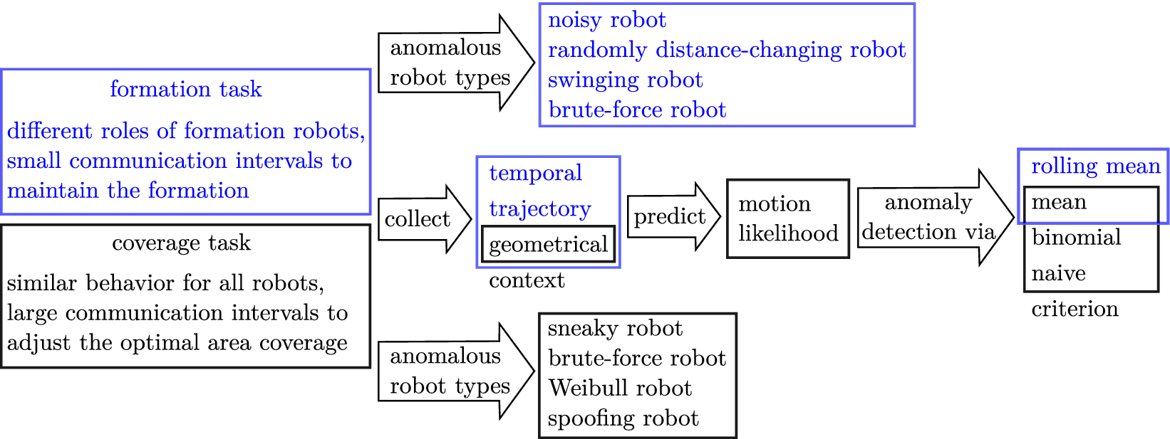
Novel contributions of this work are the transfer of the detection method in Wenger et al. (Reference Wenger, Ebel and Eberhard2026) to the alternative problem setting of moving robot formations, thereby requiring significant changes to the robots’ situational context, for instance, by including a temporal component into the context. Furthermore, several strategies of anomalous or antagonistic behavior of formation members are developed and implemented in this work to evaluate the performance of the detection approach, and a novel detection criterion used for categorizing the robots is investigated. An overview of novel contributions is shown in Figure 1.
Novelties (in blue) of this paper compared to the scenario and method in Wenger et al. (Reference Wenger, Ebel and Eberhard2026).
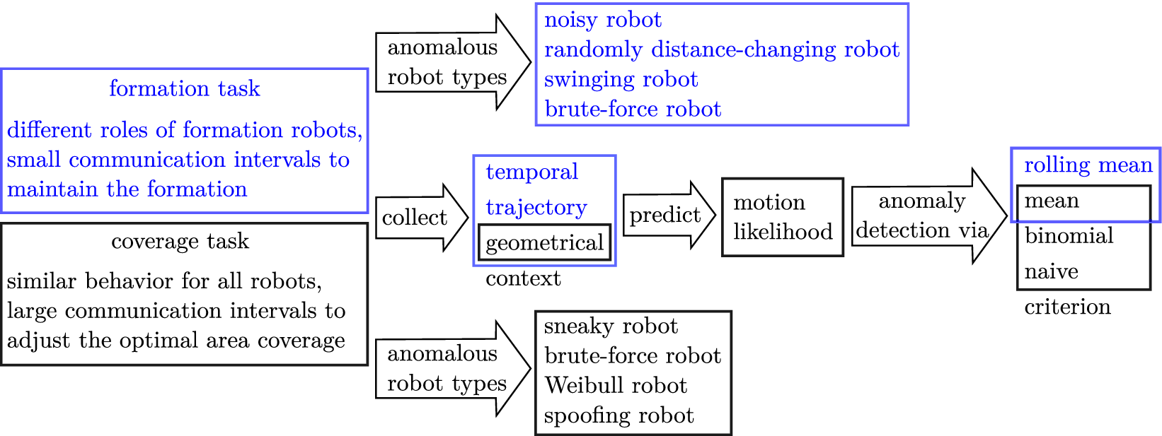
Figure 1. Long description
In the coverage task, all robots behave similarly and communication intervals are large, as they are only used to adjust the optimal area coverage. In contrast, robots have different roles during a formation task and small communication intervals are needed to maintain the formation. The context collected for the coverage task comprises only geometrical information, while the formation task also uses temporal and trajectory information. Based on the context, a motion likelihood is predicted. The anomaly detection criteria evaluated for the coverage task are the mean, binomial, and naive criterion, while the formation task uses the mean and a rolling mean criterion. Additionally, the formation task uses different types of anomalous robots, which are called noisy, randomly distance-changing, swinging and brute-force robot.
The paper is structured as follows. In Section 2, the chosen formation control approach is described and different anomalous behavior patterns and antagonistic strategies are derived from the formation structure. Section 3 revisits the detection architecture from Wenger et al. (Reference Wenger, Ebel and Eberhard2026) and includes the necessary adjustments for the new problem setting. Details on the setup of the simulation experiments are provided in Section 4. Section 5 evaluates the detection approach of a dataset of robot formations that includes antagonistic robots.
2. Anomalous agents in a formation task
Formation control is a key problem in swarm robotics, and extensive research is available having a multitude of variations and adaptations to different task requirements. For instance, a group of robot agents can be controlled by a central control unit or by distributing the control task among all group members. Similarly, the movement of the formation can either be directed by one (Kang and Ahn, Reference Kang and Ahn2018; Ahn, Reference Ahn2020) or multiple (Vu et al., Reference Vu, Trinh, Van Tran and Ahn2024) assigned leaders (leader–follower control) or by consensus of all formation members (Ebel, Reference Ebel2021). Commonly used strategies to control the movement of multiagent formations are graph-based control schemes (Ebel, Reference Ebel2021), distributed model predictive control (Ebel, Reference Ebel2021), or the use of artificial force fields (Dang et al., Reference Dang, La, Nguyen and Horn2019), with each approach offering distinct trade-offs in terms of complexity, control performance, and the required communication among formation members.
Graph-based formation control approaches are relatively simplistic and generally do not require communication between formation members, except for their pose, i.e., their position and orientation. Distance-only graph-based formation control approaches further simplify the communication by relying solely on relative positional measurements, which allows them to be easily implemented in a distributed way. However, maintaining a specific orientation of the overall formation in the global reference frame can be difficult to achieve when only the relative distances between agents are controlled to the desired values (Kang and Ahn, Reference Kang and Ahn2018).
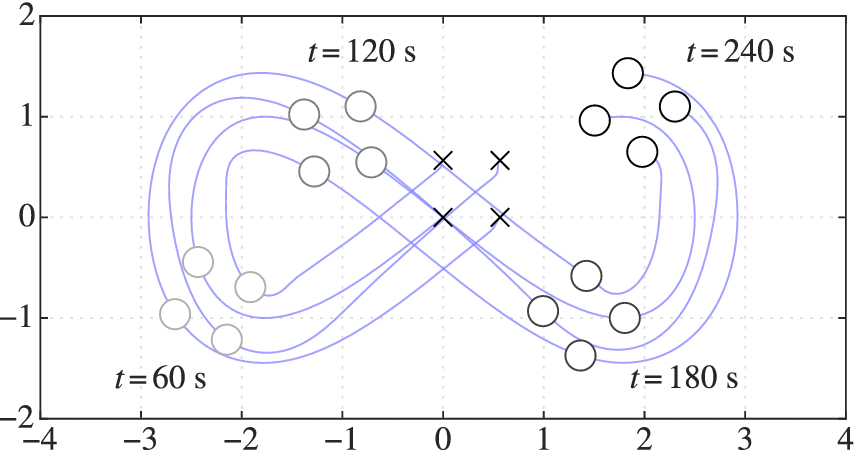
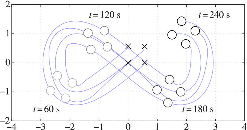
Therefore, in this work, a modified distance-based formation control scheme, as proposed in Kang and Ahn (Reference Kang and Ahn2018), is applied. The proposed approach controls both the desired formation shape and the orientation of the formation relative to its motion direction, while the formation follows a predefined trajectory; see the example illustrated in Figure 2. The approach is decentralized and the motion is directed via the leader-follower control.
Trajectory of a robot formation with controlled shape and orientation.
2.1. Employed formation control scheme
The formation control approach proposed in Kang and Ahn (Reference Kang and Ahn2018) presumes each formation member to follow single integrator dynamics, i.e.,
$ \dot{\mathbf{x}}=\mathbf{u} $
 . Although the approach is later applied to a more complex multibody model, as described in Section 4.1, this assumption is common for the nominal kinematics of omnidirectional robots.
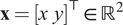
Neglecting the orientation of a robot, the state vector
$ \mathbf{x}={\left[x\hskip0.5em y\right]}^{\top}\in {\mathrm{\mathbb{R}}}^2 $
 only includes the robot position. The control input
$ \mathbf{u} $
only includes the robot position. The control input
$ \mathbf{u} $
 and the velocity
$ \mathbf{v} $
and the velocity
$ \mathbf{v} $
 are consequently given by
$ \mathbf{u}={\left[\begin{array}{cc}{u}_x& {u}_y\end{array}\right]}^{\top}\in {\mathrm{\mathbb{R}}}^2 $
are consequently given by
$ \mathbf{u}={\left[\begin{array}{cc}{u}_x& {u}_y\end{array}\right]}^{\top}\in {\mathrm{\mathbb{R}}}^2 $
 and
$ \mathbf{v}={\left[\begin{array}{cc}{v}_x& {v}_y\end{array}\right]}^{\top}\in {\mathrm{\mathbb{R}}}^2 $
and
$ \mathbf{v}={\left[\begin{array}{cc}{v}_x& {v}_y\end{array}\right]}^{\top}\in {\mathrm{\mathbb{R}}}^2 $
 . The relative distance vector between two agents
$ i $
. The relative distance vector between two agents
$ i $
 and
$ j $
and
$ j $
 is defined as
$ {\mathbf{z}}_{j,i}={\mathbf{x}}_j-{\mathbf{x}}_i\in {\mathrm{\mathbb{R}}}^2 $
is defined as
$ {\mathbf{z}}_{j,i}={\mathbf{x}}_j-{\mathbf{x}}_i\in {\mathrm{\mathbb{R}}}^2 $
 and
$ {d}_{j,i}\in \mathrm{\mathbb{R}} $
and
$ {d}_{j,i}\in \mathrm{\mathbb{R}} $
 denotes the desired distance between two robots.
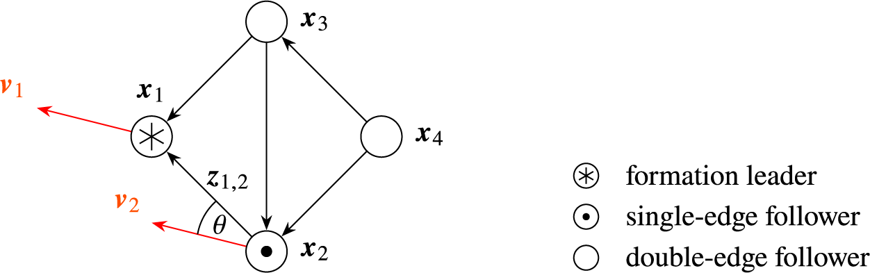
An example formation is shown in Figure 3. The formation graph
$ \mathcal{G}=\left(\mathcal{V},\mathcal{G}\right) $
 is defined by a set of vertices
$ \mathcal{V}=\left\{1,\dots, N\right\} $
is defined by a set of vertices
$ \mathcal{V}=\left\{1,\dots, N\right\} $
 , given by the robots of which the formation is composed, and a set of directed edges
$ \mathrm{\mathcal{E}}=\left\{\dots, \left(i,j\right),\dots \right\}\subseteq \mathcal{V}\times \mathcal{V} $
, given by the robots of which the formation is composed, and a set of directed edges
$ \mathrm{\mathcal{E}}=\left\{\dots, \left(i,j\right),\dots \right\}\subseteq \mathcal{V}\times \mathcal{V} $
 . Following Kang and Ahn (Reference Kang and Ahn2018), the graph is assumed to be acyclic and persistent.
Structure of the formation graph.
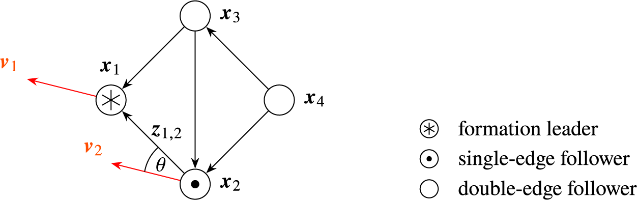
Figure 3. Long description
The formation leader has no outgoing edge. The single-edge follower has one edge to the leader. Its motion vector is parallel to the motion vector of the leader, with an angle theta from the edge to the motion vector. The third and fourth robots are double-edge followers, with two edges to the leader and single-edge follower, and the single-edge follower and the third robot, respectively.
The overall control scheme aims to solve the shape problem,


as well as the orientation problem,

where
$ {\theta}_{\mathrm{d}} $
 denotes the desired value for the angle
$ \theta \in \mathrm{\mathbb{R}} $
denotes the desired value for the angle
$ \theta \in \mathrm{\mathbb{R}} $
 between the formation’s motion vector and
$ {\mathbf{z}}_{1,2} $
between the formation’s motion vector and
$ {\mathbf{z}}_{1,2} $
 .
.
In accordance with the number of outgoing edges connected to a robot, the formation members can be divided into three distinct types that follow different control laws. The formation leader has no outgoing edges in the formation graph and is responsible for guiding the robot swarm along a predefined path. In principle, any trajectory tracking controller can be utilized to achieve path following. However, for single integrator dynamics, a simple go-to-goal controller is sufficient, which steers the robot with a constant speed
$ {v}_1=\parallel {\mathbf{v}}_1\parallel \in \mathrm{\mathbb{R}} $
 in the direction of the current goal position on the desired trajectory.
Equation (2.3) indicates the role of the second robot type, which is to maintain the orientation of the formation in the global frame. Robots of this type have one outgoing edge and are called single-edge followers. The controller of the single-edge follower approximates and matches the velocity vector
$ {\mathbf{v}}_1 $
 of the formation leader, uses a gradient-based distance control, and ensures the correct edge alignment relative to the direction of movement of the formation leader.
All remaining robots in a formation belong to the third robot type, called double-edge follower. They are attached to the formation graph by two outgoing edges to two different formation robots, controlling the velocity and distance to both robots. The given control scheme only requires the communication of individual robot positions in the global frame of reference, therefore preserving one of the great advantages of distance-based approaches. A detailed description of the control laws and the estimator mechanics, as well as a stability analysis, can be found in Kang and Ahn (Reference Kang and Ahn2018). It needs to be mentioned that the stability proof in Kang and Ahn (Reference Kang and Ahn2018) does not consider constraints on the control input, which will inevitably be encountered when modeling and working with real robot hardware. As it is not the scope of this work to provide a provably stable formation control scheme and the employed one is merely used for generating simulation data, this problem will be circumvented by practical considerations such as restricting the number of robots, the distance between robots, and the velocity of the formation leader.
2.2. Anomalous agents as formation members
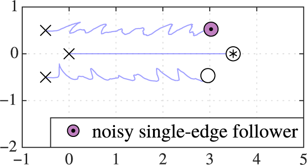
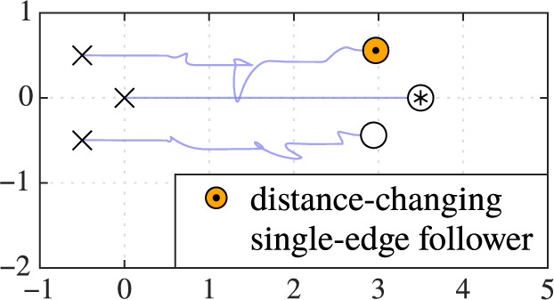
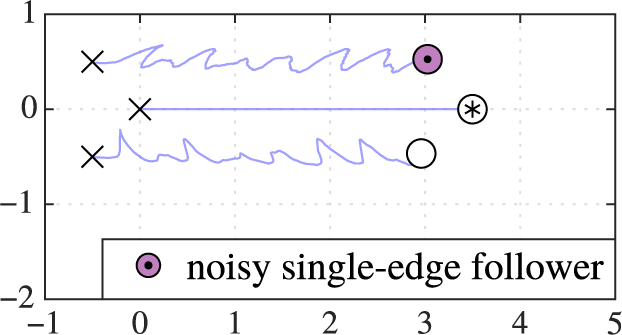
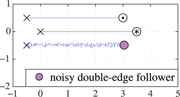
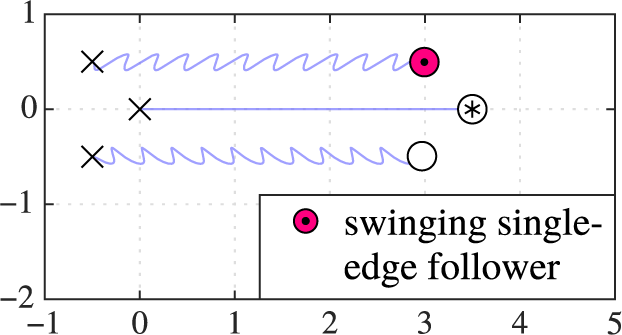
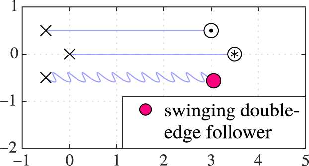
Graph-based formation control schemes pose an interesting challenge for the detection of anomalies, as any faulty action is propagated through the formation graph, possibly affecting agents directly or indirectly connected to the anomalous agent, and disrupting formation stability. This effect of propagating anomalous behavior can be observed in the left column of Figure 4.
Anomalous and antagonistic robots as formation members.
Robot formation with noisy single-edge follower.
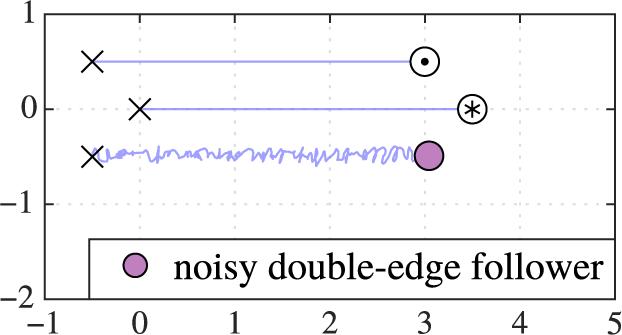
Robot formation with noisy double-edge follower.
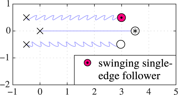
Robot formation with swinging single-edge follower.
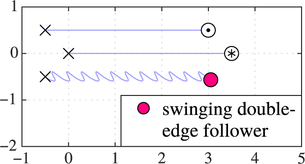
Robot formation with swinging double-edge follower.
Robot formation with randomly distance-changing single-edge follower.
Robot formation with randomly distance-changing double-edge follower.
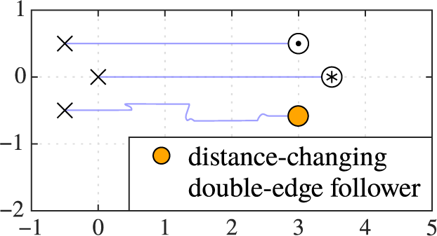
Figure 4. Long description
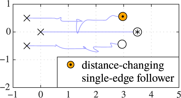
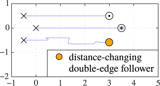
Visualization of the noisy, swinging, and distance-changing behaviors. The images show a formation of three robots, with the leader performing a horizontal movement of 3.5 metres to the right. Each type of anomaly is separately visualized for an anomalous double-edge follower, and for an anomalous single-edge follower, in which case the double-edge follower is also influenced by the anomalous movement.
For the investigation and evaluation conducted in this work, three examples of anomalous behavior are designed and implemented, and the anomalous behavior is executed by a single formation member, being either a single-edge or a double-edge follower. One reason for the anomalous behavior of a formation member can be hardware or software malfunctions. For instance, the first anomalous robot type, called noisy robot, is affected by communication noise that interferes with the incoming position information. As depicted in Figure 4a,b, the robot consequently operates on inaccurate data that causes erratic movement.
Whereas jittering and chaotic movement caused by noisy communication can already endanger formation integrity, antagonistic robots might try to actively destroy the formation by provoking collisions or executing specific motion patterns. The latter approach is pursued by the second anomalous robot, called swinging robot. As shown in Figure 4c,d, the robot adds a swinging motion to its regular following behavior, with the aim of throwing off other robots connected to itself via graph edges as a sabotage maneuver. This is particularly interesting from a system theoretic standpoint, as graph-based controlled formations in a sense resemble flexible structures. By adjusting the amplitude and the frequency of the swinging motion, the antagonistic robot can try to find a movement pattern that the formation structure is particularly sensitive against, comparable to resonance frequencies of mechanical structures.
A third type of irregular behavior entails a formation member abruptly changing its position inside the formation by actively altering the desired alignment angle or the distance to the other robots in the graph (see Figure 4e,f). The behavior of this third, randomly distance-changing robot can stem from software issues or be the cause of a hostile takeover of the robot. To achieve a persisting anomalous behavior, as for the other two anomaly types, the position changes occur repeatedly.
3. Detection of anomalous formation members
The challenge of detecting anomalous motion behavior of swarm robots without formation in the context of a coverage problem is thoroughly addressed in Wenger et al. (Reference Wenger, Ebel and Eberhard2025, Reference Wenger, Ebel and Eberhard2026). This work aims to apply the proposed method to the formation control scenario described in Section 2, where a robot swarm is assigned to move along a trajectory while maintaining a geometrical formation. The categorization of the formation members as normal or anomalous in the formation scenario requires an evaluation of the robots’ physical motions. The motion behavior of a mobile robot is represented by the robot’s change in position during a time interval
$ \Delta {t}_{\mathrm{d}} $
 , and is referred to as the robot’s actions.
As in the referenced work (Wenger et al. Reference Wenger, Ebel and Eberhard2025, Reference Wenger, Ebel and Eberhard2026), a contextual anomaly detection approach is utilized, as the robot’s actions depend on the observed situational context, e.g., on the robot’s position in the formation. An overview of the design choices for the representation of context in a formation task is found in Section 3.1.
Similar to Wenger et al. (Reference Wenger, Ebel and Eberhard2025, Reference Wenger, Ebel and Eberhard2026), the detection approach should not be restricted to signatures or prior knowledge of anomalous behavior. Instead, a formation member is categorized as anomalous if its behavior seems to be unlikely in comparison to the expected normal behavior. Thus, a dataset containing the actions and the context observed in simulations of correctly behaving robots is used to define a reference point for the normal robot behavior. This dataset can be assumed to comprise samples of an underlying distribution
$ {p}_{\mathbf{a}}^{\ast } $
 , where normal robot behavior corresponds to regions with a high probability density (Chandola et al., Reference Chandola, Banerjee and Kumar2009). Based on the probability density value, or likelihood, of a robot action, an anomaly score can be estimated for this action. Section 3.2 contains a brief overview of how the anomaly score can be approximated by training a neural network on the dataset containing simulations of normal robot behavior.
In a final step, the robot is categorized as normal or anomalous. This is done by evaluating the robot behavior based on a detection criterion that uses the predicted anomaly score of several robot actions, as described in Section 3.3.
3.1. Describing the context of robots in the formation setting
It is a fundamental problem faced when training generative models, like normalizing flows, to find a context description that carries sufficient information for the model to learn the target distribution. In the formation scenario, this means that the situational context
$ \boldsymbol{s} $
 is required to adequately describe the current state of the formation, so that the likelihood of a robot’s next action can be reliably estimated. However, the information that is made available to the network undergoes some restrictions, as the context representation should neither be limited to information that is specific to the controller architecture and mechanisms, nor require access to the formation graph and the formation geometry. Thus, the following four sets of context information were found to be easily available and to improve the training and validation performance of the neural network (for details see Ziegler, Reference Ziegler2025).
As required by the formation control approach, each formation member communicates its own position to the other robots. Thus, the position information is included by computing the relative distance vectors from a robot’s position to the positions of all other formation members. Furthermore, the geometrical center of the formation can be calculated from the robot positions, extending the situational context by the relative distance vector from a robot’s position to the current position of the formation center. These distance vectors consequently capture geometrical information, which is used to predict the robot motion relative to each neighbor. However, as a robot’s motion depends on the direction of motion of the entire formation, as well as the robot’s current speed and momentum, a temporal context component is required. This temporal context is added by including a robot’s distance vector to its own position at a previous time step, i.e., the robot’s previous action. Additionally, if the leader’s future trajectory is known and accessible, it can be incorporated into the context description to provide information on the future location of the robot formation. In this work, the future trajectory is included as the distance between a robot’s position and a look-ahead point on the leader trajectory.
The preprocessing of the action and the context into features that are passed to the neural network is done similar to Wenger et al. (Reference Wenger, Ebel and Eberhard2026), where each of the relative distance or motion vectors is preprocessed into a three-dimensional feature comprising the normalized vector and the scaled magnitude of the vector. The resulting context
$ \boldsymbol{s}\in {\mathrm{\mathbb{R}}}^{n_{\mathrm{s}}\times 3} $
 is passed into a bidirectional Long Short-Term Memory (LSTM) (Hochreiter and Schmidhuber, Reference Hochreiter and Schmidhuber1997; Schuster and Paliwal, Reference Schuster and Paliwal1997), in order to compute a fixed-size context embedding.
3.2. Learning action likelihoods through the use of normalizing flows
The anomaly score of an action
$ \boldsymbol{a}\in {\mathrm{\mathbb{R}}}^{n_{\mathrm{a}}\times 3} $
 performed by a robot given the situational context
$ \boldsymbol{s} $
performed by a robot given the situational context
$ \boldsymbol{s} $
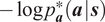
 can be defined as the negative log likelihood
$ -\log {p}_{\boldsymbol{a}}^{\ast}\left(\boldsymbol{a}\hskip0.1em |\hskip0.1em \boldsymbol{s}\right) $
can be defined as the negative log likelihood
$ -\log {p}_{\boldsymbol{a}}^{\ast}\left(\boldsymbol{a}\hskip0.1em |\hskip0.1em \boldsymbol{s}\right) $
 under the true distribution
$ {p}_{\boldsymbol{a}}^{\ast } $
under the true distribution
$ {p}_{\boldsymbol{a}}^{\ast } $
 representing normal robot behavior. As the probability density
$ {p}_{\boldsymbol{a}}^{\ast } $
representing normal robot behavior. As the probability density
$ {p}_{\boldsymbol{a}}^{\ast } $
 is not directly accessible in practice, a normalizing flow model (Rezende and Mohamed, Reference Rezende and Mohamed2015) is utilized as an estimator for the likelihood of context–action pairs. Normalizing flows are neural networks with the ability to approximate unknown probability densities by learning suitable model parameters
$ \boldsymbol{\theta} $
is not directly accessible in practice, a normalizing flow model (Rezende and Mohamed, Reference Rezende and Mohamed2015) is utilized as an estimator for the likelihood of context–action pairs. Normalizing flows are neural networks with the ability to approximate unknown probability densities by learning suitable model parameters
$ \boldsymbol{\theta} $
 , which maximize the likelihood of the samples provided in the training data. Thus, if the flow is being trained on data of normal robot behavior, it assigns a high likelihood to normal robot actions and a lower likelihood to unknown, abnormal actions. A detailed explanation of the structure and learning mechanisms of normalizing flows can be found in Papamakarios et al. (Reference Papamakarios, Nalisnick, Rezende, Mohamed and Lakshminarayanan2021).
Starting from a base distribution
$ {p}_{\boldsymbol{u}} $
 , e.g., a normal or uniform distribution, the neural network learns a set of differentiable and invertible transformation functions
$ {\boldsymbol{T}}_k $
, e.g., a normal or uniform distribution, the neural network learns a set of differentiable and invertible transformation functions
$ {\boldsymbol{T}}_k $
 that compute a transformation from
$ {p}_{\boldsymbol{u}} $
that compute a transformation from
$ {p}_{\boldsymbol{u}} $
 to
$ {p}_{\boldsymbol{a}} $
to
$ {p}_{\boldsymbol{a}} $
 via their composition
$ \boldsymbol{T}={\boldsymbol{T}}_K\circ \dots \circ {\boldsymbol{T}}_1 $
via their composition
$ \boldsymbol{T}={\boldsymbol{T}}_K\circ \dots \circ {\boldsymbol{T}}_1 $
 . This work uses spline-based transformer functions
$ {\boldsymbol{T}}_k $
. This work uses spline-based transformer functions
$ {\boldsymbol{T}}_k $
 , where the properties characterizing the splines depend on the current context embedding
$ \boldsymbol{s} $
, where the properties characterizing the splines depend on the current context embedding
$ \boldsymbol{s} $
 that is passed from the LSTM.
The probability density value for an action
$ \boldsymbol{a} $
 , given the context
$ \boldsymbol{s} $
, given the context
$ \boldsymbol{s} $
 , is then computed as

where
$ {\boldsymbol{J}}_{{\boldsymbol{T}}^{-1}} $
 is the Jacobian matrix of the inverse transformation function with respect to
$ \boldsymbol{a} $
is the Jacobian matrix of the inverse transformation function with respect to
$ \boldsymbol{a} $
 . To approximate the true data distribution
$ {p}_{\boldsymbol{a}}^{\ast } $
. To approximate the true data distribution
$ {p}_{\boldsymbol{a}}^{\ast } $
 , the neural network maximizes the probability density values of the training samples
$ \boldsymbol{a}\sim {p}_{\boldsymbol{a}}^{\ast } $
, the neural network maximizes the probability density values of the training samples
$ \boldsymbol{a}\sim {p}_{\boldsymbol{a}}^{\ast } $
 under the model distribution
$ {p}_{\boldsymbol{a}} $
under the model distribution
$ {p}_{\boldsymbol{a}} $
 . This can equivalently be done by minimizing the Kullback–Leibler divergence between
$ {p}_{\boldsymbol{a}}^{\ast } $
. This can equivalently be done by minimizing the Kullback–Leibler divergence between
$ {p}_{\boldsymbol{a}}^{\ast } $
 and
$ {p}_{\boldsymbol{a}} $
and
$ {p}_{\boldsymbol{a}} $
 (Papamakarios et al., Reference Papamakarios, Nalisnick, Rezende, Mohamed and Lakshminarayanan2021), i.e., by minimizing

The transformation function
$ \boldsymbol{T} $
 can be further used to sample from
$ {p}_{\boldsymbol{a}} $
can be further used to sample from
$ {p}_{\boldsymbol{a}} $
 by transforming samples
$ {\boldsymbol{u}}_{\boldsymbol{s}}\sim {p}_{\boldsymbol{u}} $
by transforming samples
$ {\boldsymbol{u}}_{\boldsymbol{s}}\sim {p}_{\boldsymbol{u}} $
 from the base distribution, i.e.,
$ {\boldsymbol{a}}_{\boldsymbol{s}}=\boldsymbol{T}\left({\boldsymbol{u}}_{\boldsymbol{s}}\right) $
from the base distribution, i.e.,
$ {\boldsymbol{a}}_{\boldsymbol{s}}=\boldsymbol{T}\left({\boldsymbol{u}}_{\boldsymbol{s}}\right) $
 .
.
As in Wenger et al. (Reference Wenger, Ebel and Eberhard2026), a non-autoregressive coupling flow is employed, and the Python package nflows (Durkan et al., Reference Durkan, Bekasov, Murray and Papamakarios2020) is utilized to construct the normalizing flow model. (For further information on the network architecture and training, refer to Section 4.2.)
3.3. Finding likelihood thresholds for the detection of anomalous formation members
In the prior work (Wenger et al., Reference Wenger, Ebel and Eberhard2026), several criteria were introduced for categorizing a robot as anomalous given its performed actions and their estimated likelihoods. One of the proposed criteria is the categorization of a robot based on the mean of the estimated likelihoods of all its observed actions
$ {\mathbf{a}}_{\mathrm{o}} $
 . Derived from this approach of averaging action likelihoods, an additional detection criterion is proposed, where the mean of the action likelihoods is calculated across previously performed actions
$ {\boldsymbol{a}}_{\mathrm{RW}}=\left\{{\boldsymbol{a}}_t,{\boldsymbol{a}}_{t-1},\dots, {\boldsymbol{a}}_{t-{l}_{\mathrm{RW}}+1}\right\}\subset {\boldsymbol{a}}_{\mathrm{o}} $
. Derived from this approach of averaging action likelihoods, an additional detection criterion is proposed, where the mean of the action likelihoods is calculated across previously performed actions
$ {\boldsymbol{a}}_{\mathrm{RW}}=\left\{{\boldsymbol{a}}_t,{\boldsymbol{a}}_{t-1},\dots, {\boldsymbol{a}}_{t-{l}_{\mathrm{RW}}+1}\right\}\subset {\boldsymbol{a}}_{\mathrm{o}} $
 within a rolling window of predefined window length
$ \mid {\boldsymbol{a}}_{\mathrm{RW}}\mid ={l}_{\mathrm{RW}} $
within a rolling window of predefined window length
$ \mid {\boldsymbol{a}}_{\mathrm{RW}}\mid ={l}_{\mathrm{RW}} $
 . Consequently, a robot is categorized as anomalous if

holds, where
$ h\in \mathrm{\mathbb{R}} $
 is a tunable detection threshold. The threshold
$ h $
is a tunable detection threshold. The threshold
$ h $
 has to be chosen carefully, as it also directly impacts the number of normal robots falsely categorized as anomalous. Depending on the severity of false positive categorization,
$ h $
has to be chosen carefully, as it also directly impacts the number of normal robots falsely categorized as anomalous. Depending on the severity of false positive categorization,
$ h $
 can be adapted to provide a desired maximum false positive rate
$ {FPR}_{\mathrm{max}} $
can be adapted to provide a desired maximum false positive rate
$ {FPR}_{\mathrm{max}} $
 for robots with normal behavior, i.e.,

4. Randomized setup of formation tasks
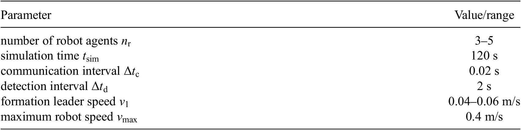
All datasets used in this work are created by simulating different randomized episodes of a formation task using the parameter setup in Table 1.
Parameters used for the collection of simulation data
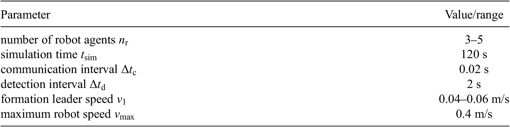
Table 1. Long description
The number of robots is between 3 and 5. The total simulation time is 120 seconds. Robots communicate in intervals of 0.02 seconds and the anomalies are detected in intervals of 2 seconds. The speed of the formation leader is 0.04 to 0.06 metres per second, while the maximum speed of a robot is limited to 0.4 metres per second.
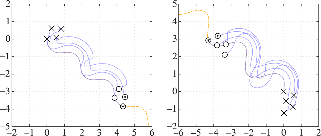
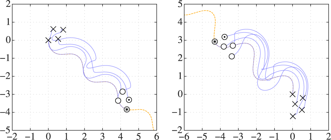
For creating the training data, in each episode the robots are placed at randomized initial positions within a bounded region, ensuring no collisions and maintaining a minimum separation distance. The relative distances and angles calculated from these initial positions define the geometrical structure of the formation maintained throughout the episode, and the randomized orientation of the robot formation determines the initial heading of the leader trajectory. The formation initialization enforces that the maximum distance between any two robots connected via a graph edge remains below a predefined threshold. This geometric constraint is necessary to ensure that the coordinated formation movement remains feasible, given the velocity limitation of the robots. Similarly, while the trajectory followed by the assigned formation leader is a randomized sinusoidal path, its curve periodicity and curvature are also constrained to comply with the robots’ maximum velocity. The sinusoidal trajectories are selected over alternative path geometries, such as lemniscates, to ensure sufficient curvature variability in the training data. Figure 5 visualizes two episodes included in the training dataset.
Robot trajectories and leader path for two episodes included in the training dataset.
To maintain the formation, the robots communicate their positions at regular small time intervals
$ \Delta {t}_{\mathrm{c}} $
 . As noisy robots are affected by communication noise, changes in their behavior can also be observed every
$ \Delta {t}_{\mathrm{c}} $
. As noisy robots are affected by communication noise, changes in their behavior can also be observed every
$ \Delta {t}_{\mathrm{c}} $
 . In contrast, the previously described behavior changes of a randomly distance-changing robot occur in larger intervals of 10s.
The anomaly detection is performed in larger detection intervals of
$ \Delta {t}_{\mathrm{d}}=100\hskip0.1em \Delta {t}_{\mathrm{c}} $
 . Thus, the robot actions passed to the network represent position changes over a time span of
$ \Delta {t}_{\mathrm{d}} $
. Thus, the robot actions passed to the network represent position changes over a time span of
$ \Delta {t}_{\mathrm{d}} $
 and the look-ahead distance for the trajectory feature corresponds to the position that the leader robot is supposed to reach after
$ \Delta {t}_{\mathrm{d}} $
and the look-ahead distance for the trajectory feature corresponds to the position that the leader robot is supposed to reach after
$ \Delta {t}_{\mathrm{d}} $
 .
.
4.1. Robot hardware and multibody model
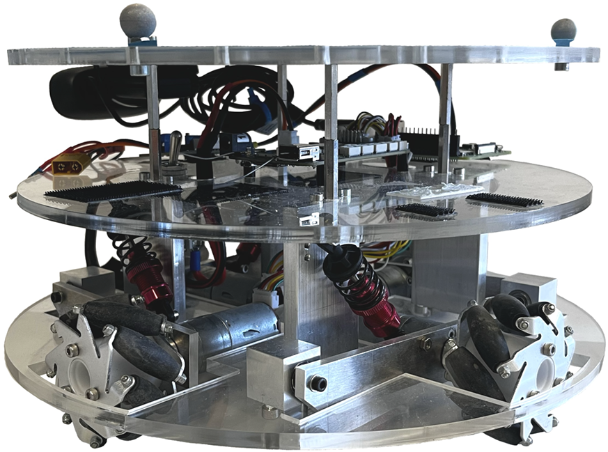
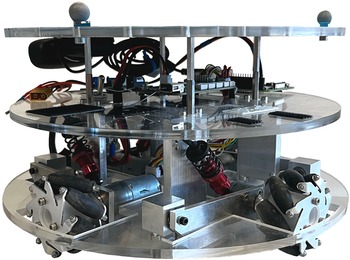
The multibody model used in simulation is derived from the robot depicted in Figure 6, which is built at the Institute for Engineering and Computational Mechanics. This robotic platform, called Holonomic Extensible Robotic Agent (HERA) (Ebel and Eberhard, Reference Ebel and Eberhard2021), is equipped with four Mecanum wheels, allowing for omnidirectional planar movement. The requested translational velocity of the robot’s center is converted into the individual angular velocities for each wheel that are required for achieving the desired movement. The angular velocity of each wheel is controlled by local motor controllers and the maximum straight line velocity of the robot is
$ 0.4\;\mathrm{m}/\mathrm{s} $
 . The multibody model of the robot can be found in Ebel (Reference Ebel2021).
Omnidirectional mobile robot (Ebel, Reference Ebel2021).
4.2. Training of the neural network and tuning of detection thresholds
The neural network is implemented in PyTorch (Paszke et al., Reference Paszke, Gross, Massa, Lerer, Bradbury, Chanan, Killeen, Lin, Gimelshein, Antiga, Desmaison, Köpf, Yang, DeVito, Raison, Tejani, Chilamkurthy, Steiner, Fang, Bai and Chintala2019) and the training workflow integrates Weights and Biases (WandB) (Biewald, Reference Biewald2020) for the experiment tracking and the hyperparameter optimization. The dataset used for training the neural network consists of 350 randomized episodes (
$ 82\hskip0.1em 541 $
 samples) of normal robot behavior following the setup described in Section 4 and the training is validated on 125 additional episodes (
$ 30\hskip0.1em 031 $
samples) of normal robot behavior following the setup described in Section 4 and the training is validated on 125 additional episodes (
$ 30\hskip0.1em 031 $
 samples) of normal behavior. The detection threshold
$ h $
samples) of normal behavior. The detection threshold
$ h $
 introduced in Section 3.3 is tuned according to Equation (3.4) on 50 additional episodes of normal robot behavior, setting
$ {FPR}_{\mathrm{max}}=0.05 $
introduced in Section 3.3 is tuned according to Equation (3.4) on 50 additional episodes of normal robot behavior, setting
$ {FPR}_{\mathrm{max}}=0.05 $
 .
.
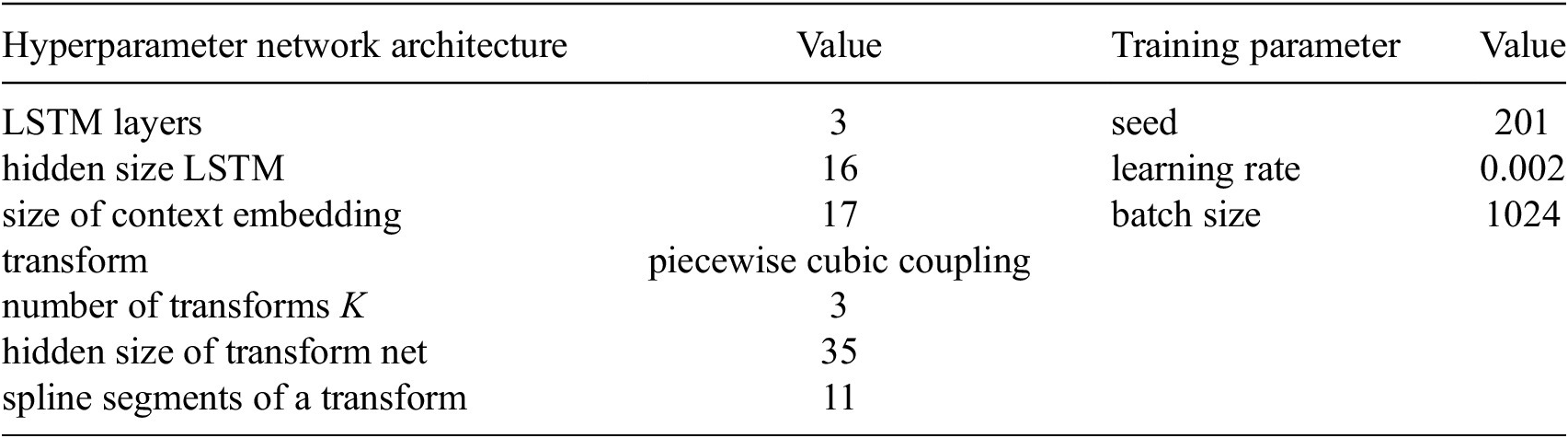
The hyperparameters of the model that performed best on the validation data are shown in Table 2.
Hyperparameters of the best model with full context information
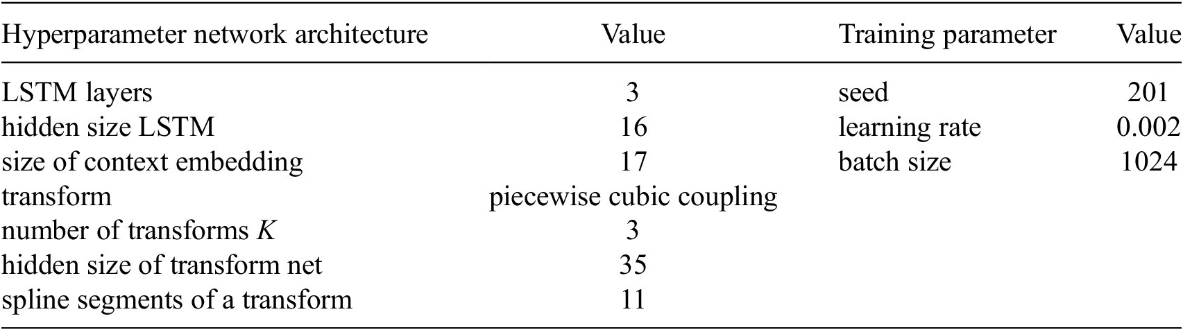
Table 2. Long description
The LSTM has 3 layers with hidden size 16 and output or context embedding size 17. The normalizing flow uses 3 piecewise cubic coupling transforms, with 11 spline segments each and a hidden size 35 of the transform networks. The network is trained with a seed of 201, a learning rate of 0.002 and a batch size of 1024.
The test dataset is used for evaluating the detection performance of the trained neural network by including both normal and anomalous robots. It consists of 500 simulated episodes for each of the anomalous robot types described in Section 2.2. In each episode of the test dataset, the robot formation includes exactly one anomalous robot at a random node of the formation graph, excluding the formation leader.
5. Results
The detection performance for the anomalous robots described in Section 2.2 is evaluated for the best neural network, i.e., the network with the highest mean validation log probability obtained during hyperparameter optimization.
The anomaly detection is performed at discrete time intervals
$ \Delta {t}_{\mathrm{d}} $
 , assigning and updating the categorization of a robot as normal (N) or anomalous (A) according to Equation (3.3). Thus, according to the number of intervals
$ \Delta {t}_{\mathrm{d}} $
, assigning and updating the categorization of a robot as normal (N) or anomalous (A) according to Equation (3.3). Thus, according to the number of intervals
$ \Delta {t}_{\mathrm{d}} $
 during an episode, several categorizations are available for each robot. To evaluate the performance of the anomaly-detection method, the following metrics are computed over all categorizations, denoted as
$ {}^{\hat } $
during an episode, several categorizations are available for each robot. To evaluate the performance of the anomaly-detection method, the following metrics are computed over all categorizations, denoted as
$ {}^{\hat } $
 , of all robots in the simulated test dataset. The specificity describes the percentage of correct categorizations of normal robots (
$ \hat{\mathrm{N}}\mid \mathrm{N} $
, of all robots in the simulated test dataset. The specificity describes the percentage of correct categorizations of normal robots (
$ \hat{\mathrm{N}}\mid \mathrm{N} $
 ), while the percentage of correctly detected anomalous robot categorizations (
$ \hat{\mathrm{A}}\mid \mathrm{A} $
), while the percentage of correctly detected anomalous robot categorizations (
$ \hat{\mathrm{A}}\mid \mathrm{A} $
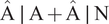
 ) is referred to as the sensitivity. The precision denotes the number of correct categorizations of anomalous robots divided by the number of all anomalous categorizations (
$ \hat{\mathrm{A}}\mid \mathrm{A}+\hat{\mathrm{A}}\mid \mathrm{N} $
) is referred to as the sensitivity. The precision denotes the number of correct categorizations of anomalous robots divided by the number of all anomalous categorizations (
$ \hat{\mathrm{A}}\mid \mathrm{A}+\hat{\mathrm{A}}\mid \mathrm{N} $
 ), such that

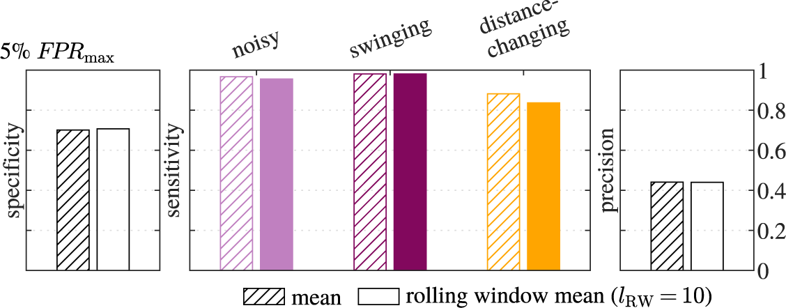
Figure 7 illustrates the resulting performance of the anomaly-detection method using the rolling window mean criterion described in Section 3.3, with a window length of
$ {l}_{\mathrm{RW}}= $
 10. Additionally, the metrics are shown for the mean criterion as an edge case of the rolling window mean criterion with a window length corresponding to all available actions.
Specificity, sensitivity, and precision results evaluated on all actions in the test dataset, using the mean detection criterion and the rolling window mean detection criterion.

The network can detect noisy, swinging, and randomly distance-changing robots with respective mean criterion categorization percentages of 96.7%, 98.1%, and 88.2%. When using the rolling window mean criterion, the percentages are slightly lower with 95.6% for the noisy robot, 98.1% for the swinging robot, and 83.7% for the randomly distance-changing robot. The lower performance for detecting randomly distance-changing robots can be explained by their behavior strategy being updated in larger intervals of 10s. As the anomalous modification of the robot’s distance to other formation members is sampled randomly, the distance might be close to normal and therefore lead to larger intervals of motion that resembles normal behavior. Using the rolling window mean criterion intensifies this issue, as previously detected, anomalous intervals might fall outside of the length of the window.
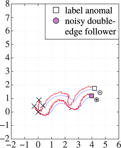
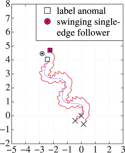
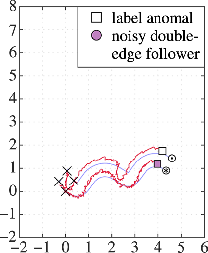
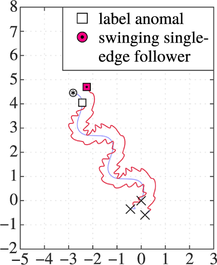
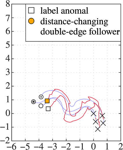
In contrast to the high sensitivity values, both the specificity and precision do not always meet the expected values considering that the detection threshold was tuned to a maximum false positive rate of 5% and should result in a specificity of at least 95%. The specificity and precision values can, however, be explained by recalling that the metrics include motions of normal robots that are affected by anomalous formation robots due to their graph edge dependencies. Figure 8 includes an episode for each of the anomalous robots to illustrate this observation. Robot trajectories are colored in red for all time intervals where a robot is categorized as anomalous.
Exemplary episodes from the detection test dataset.
Detection of the noisy robot.
Detection of the swinging robot.
Detection of the randomly distance-changing robot.

Figure 8. Long description
Qualitative results of the detection method for each type of anomaly. The anomalous robot and its followers are detected as anomalous for the entirety of their trajectories.
Thus, while the neural network is not capable of finding out which of several robots that exhibit anomalous movement patterns is the cause of the anomalies, it is generally successful in reporting robots that do not meet the expected behavior, even if they are merely influenced by the anomalous formation member. To examine whether the desired maximum false positive rate is met for robots that are neither causing nor are affected by anomalous behavior, an additional number of 500 unseen episodes is simulated, where the formations contain no anomalous robots. The resulting specificity values of 96.1% for the mean criterion and 95.2% for the rolling window mean criterion demonstrate that both detection criteria adhere to the desired maximum false positive rate of 5%.
5.1. Out-of-distribution context
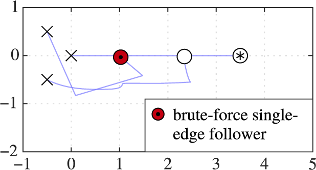
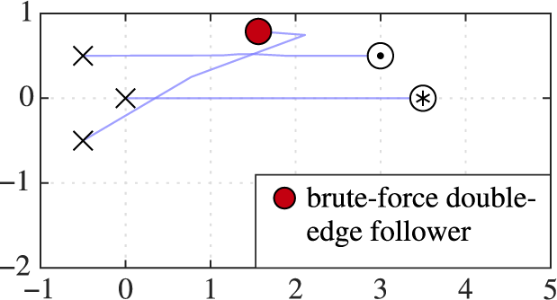
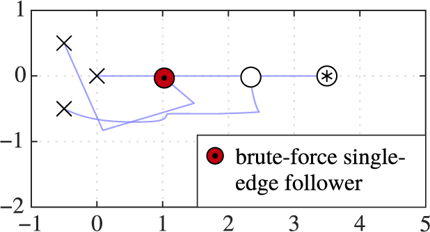
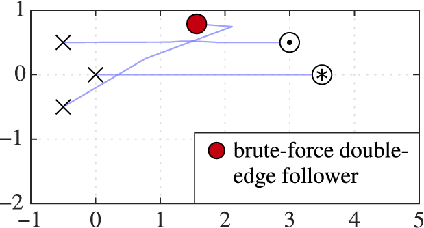
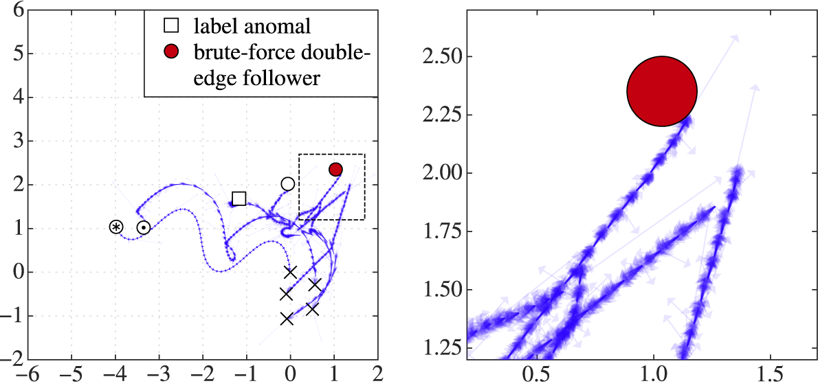
When performing the anomalous strategies described in Section 2.2, the anomalous robots continue to execute a formation-following behavior. However, an antagonistic agent could also refuse to participate in the formation task by leaving its assigned position inside the formation and moving to a different position of interest. This behavior is demonstrated by a fourth anomalous robot type, called brute-force robot, shown in Figure 9a,b. Depending on the topology of the formation graph, this behavior can break the desired robot formation apart, as, without appropriate countermeasures, other robots connected to the brute-force robot continue to coordinate their own movement based on the position of their antagonistic neighbor. It must be kept in mind that this is only a theoretically interesting case. If a brute-force antagonist completely dismantles the formation, a simple formation check is sufficient to detect this, and an elaborate anomaly-detection method is not needed. Regardless, it is interesting to investigate how the method reacts to this out-of-distribution situation.
Brute-force antagonistic robots as formation members.
Robot formation with brute-force single-edge follower.
Robot formation with brute-force double-edge follower.
A performance evaluation of the detection method on 500 randomized episodes containing a brute-force robot reveals that the antagonist can only be detected in
$ 8.7\% $
 and
$ 11.9\% $
and
$ 11.9\% $
 of the categorizations provided by the mean criterion and by the rolling window mean criterion. When investigating the reason for the method’s inability to detect this seemingly obvious antagonistic behavior, it is found that the results can be attributed to the fact that the neural network is faced with out-of-distribution context information. Out-of-distribution context information refers to a situational context that was never encountered in the training data. As such, whenever a robot drifts away from the formation, three of the four context features, i.e., the relative distance to the neighbors, the formation center, and the trajectory, deviate significantly from the usual ranges seen in training, and only the previous action feature falls within the range of values seen during training. The resulting action distributions that are predicted by the neural network for the brute-force behavior, and that are visualized as action samples, are depicted in Figure 10.
Action samples for an episode with a brute-force robot.
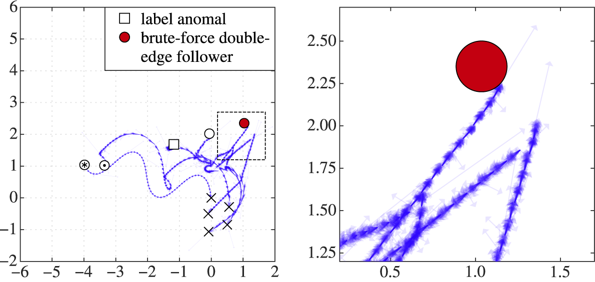
Figure 10. Long description
The third robot is a brute-force double-edge follower moving away from the formation. Only one of its followers is categorized as anomalous. The action samples shown for the brute-force robot predict that its motion continues into the same direction as for the last step.
Comparable problems with out-of-distribution data and normalizing flows were encountered and investigated in Hong et al. (Reference Hong, Park and Chun2023) and Kirichenko et al. (Reference Kirichenko, Izmailov and Wilson2020). As it is unpredictable how the neural network generalizes to out-of-distribution context, the likelihood estimates of actions given an unseen situation should generally be regarded as unreliable.
6. Conclusion
The results show that the state-of-the-art approach for data-based contextual anomaly detection of physically anomalous and antagonistic behavior performed by robots in a robot swarm can be transferred from the previously investigated deployment problem to the setting of moving robot formations, underlining its flexibility and adaptability to new swarm scenarios.
Considering only robots that execute anomalous behavior that does not lead to out-of-distribution context, the robots are correctly categorized as anomalous during 83% to 98% of their motions. Similarly, more than 95% of the motions of normally behaving agents are correctly categorized.
The presented anomaly-detection approach is likely to categorize normal robots as anomalous if their movement is affected by the actions of an anomalous robot. While this procedure can be intended, since the affected robots’ behavior also shows anomalies, it could be desirable to identify the cause of the anomalous behavior, namely, the truly anomalously acting robot. If information about the formation graph is available, the formation structure and the dependencies between the robots can be analyzed. As the formation graph is acyclic, a normal robot can only be affected by anomalous behavior if the graph contains a directed path from the normal robot to the anomalously behaving robot. Thus, the identity of the robot that is causing the anomalous behavior could be inferred by observing the propagation of anomalous motions within the graph. A similar effect might be achieved by instructing the formation to restructure the edges of the formation graph or redistributing the assigned roles of the formation members. While this approach poses a different, interesting challenge, as the new formations must conform to the employed formation control structure, it can also be investigated as a countermeasure in future work, either to mitigate the effect of anomalous motions or to exclude the anomalous robot from the formation.
As expected, an evaluation of the detection performance revealed that the reliability of the normalizing flow is limited when trying to generalize to unseen context information. A possible solution to this issue is the use of a second neural network to detect situations that translate to out-of-distribution context (OOD detection), in order to decide whether the action likelihoods estimated by the normalizing flow can be trusted. Alternatively, the likelihood for both the context and the action could be learned by a normalizing flow. As a very simple, practical solution, a robot that exceeds a predefined maximum distance to the other formation members can directly be categorized as anomalous.
While the setup of hardware experiments can be done similar to Wenger et al. (Reference Wenger, Ebel and Eberhard2026), the formation setting requires tightly scheduled and reliable communication, the addition of a collision avoidance mechanism (Ziegler, Reference Ziegler2025), and a stronger focus on proving formation stability (Kang and Ahn, Reference Kang and Ahn2018). As the robot motions might be noisier, e.g., due to friction or message loss, anomalies in the robots’ behavior might need to be accentuated in order to be distinguishable from normal motions. Thus, the transfer from simulation to hardware is another interesting topic for future research.
Supplementary material
The supplementary material for this article can be found at http://doi.org/10.1017/dce.2026.10059.
Data availability statement
Code for training and applying the described anomaly-detection method is available on GitHub (https://github.com/Institute-Eng-and-Comp-Mechanics-UStgt/AntagonisticAgents). The data used in this work is made available on DaRUS (Ziegler, Reference Ziegler, Wenger and Eberhard2025). Videos of the formation behavior and categorization are provided in the supplementary material.
Author contribution
Conceptualization: P.Z.; I.W.; P.E. Data Curation: P.Z. Formal Analysis: P.Z. Funding Acquisition: P.E. Investigation: P.Z. Methodology: P.Z.; I.W. Project Administration: P.E. Resources: P.E. Software: P.Z.; I.W. Supervision: I.W.; P.E. Validation: P.Z. Visualization: P.Z.; I.W. Writing Original Draft: P.Z.; I.W. Writing Review and Editing: P.Z.; I.W.; P.E. All authors approved the final submitted draft.
Funding statement
This research was supported by the Deutsche Forschungsgemeinschaft (DFG, German Research Foundation) under Germany’s Excellence Strategy—EXC 2075–390,740,016, project PN4–4 “Learning from Data—Predictive Control in Adaptive Multi-robot Scenarios” as well as project EB195/32–1, 433,183,605 “Research on Multibody Dynamics and Control for Collaborative Elastic Object Transportation by a Heterogeneous Swarm with Aerial and Land-Based Mobile Robots,” and project EB195/40–1, 501,890,093 “Mehr Intelligenz wagen–Designassistenten in Mechanik und Dynamik (SPP 2353).” The funders had no role in study design, data collection and analysis, decision to publish, or preparation of the manuscript.
Competing interests
The authors declare none.
Ethical standard
The research meets all ethical guidelines, including adherence to the legal requirements of the study country.


 Open access


Comments
No Comments have been published for this article.