


1. Introduction
A growing body of evidence suggests that ice mélange, a dense pack of icebergs, brash ice and sea ice, plays an important role in glacier–fjord systems by inhibiting calving of icebergs and affecting where and when meltwater is released into fjords. Ice mélange forms when ocean currents or surface winds are unable to efficiently evacuate icebergs from a proglacial fjord. The persistence of ice mélange varies significantly between fjords. For example, in the Uummannaq district of West Greenland (Howat and others, Reference Howat, Box, Ahn, Herrington and McFadden2010; Walter and others, Reference Walter2012) and the Wilkins Ice Shelf area in Antarctica (Humbert and Braun, Reference Humbert and Braun2008), ice mélange appears to exist only when air and water temperatures are low enough to permit the growth of a thick sea ice matrix that binds icebergs together. However, ice mélange can also exist without substantial sea ice coverage if iceberg productivity is sufficiently high, such as at Jakobshavn Isbræ, Helheim Glacier and Kangerdlugssuaq Glacier, Greenland. At these glaciers, ice mélange is held together by iceberg–iceberg and iceberg–bedrock contact forces (Joughin and others, Reference Joughin2008; Amundson and others, Reference Amundson2010; Seale and others, Reference Seale, Christoffersen, Mugford and O'Leary2011; Jakobsson and others, Reference Jakobsson2012; Amundson and Burton, Reference Amundson and Burton2018), although sea ice growth in winter likely provides additional rigidity (Cassotto and others, Reference Cassotto, Fahnestock, Amundson, Truffer and Joughin2015; Robel, Reference Robel2017; Bevan and others, Reference Bevan, Luckman, Benn, Cowton and Todd2019; Joughin and others, Reference Joughin, Shean, Smith and Floricioiu2020).
Several observations suggest that ice mélange can be viewed as weak, granular ice shelves that transmit stresses to glacier termini and influence iceberg calving. First, iceberg calving rates are often well-correlated with the formation and dispersal of ice mélange (or strengthening and weakening, if the ice mélange persists year round) (Sohn and others, Reference Sohn, Jezek and van der Veen1998; Reeh and others, Reference Reeh, Thomas, Higgins and Weidick2001; Joughin and others, Reference Joughin2008; Amundson and others, Reference Amundson2010; Howat and others, Reference Howat, Box, Ahn, Herrington and McFadden2010; Seale and others, Reference Seale, Christoffersen, Mugford and O'Leary2011; Walter and others, Reference Walter2012; Xie and others, Reference Xie, Dixon, Holland, Voytenko and Vaňková2019). Second, during periods of glacier terminus quiescence, ice mélange is pushed from behind by the glacier terminus at roughly the glacier flow speed (i.e., the ice mélange must also push back against the terminus) and motion is accommodated by shear bands along the fjord margins and deformation within the ice mélange (Joughin and others, Reference Joughin2008; Amundson and others, Reference Amundson2010; Sundal and others, Reference Sundal2013; Foga and others, Reference Foga, Stearns and van der Veen2014; Amundson and Burton, Reference Amundson and Burton2018). Third, complete dispersal of ice mélange appears to cause a small increase in glacier velocity that is comparable to tidally-induced velocity variations (Walter and others, Reference Walter2012). Importantly, the resistive force from ice mélange does not need to be large to hold together a heavily fractured terminus (Reeh and others, Reference Reeh, Thomas, Higgins and Weidick2001; Amundson and others, Reference Amundson2010; Krug and others, Reference Krug, Durand, Gagliardini and Weiss2015) or prevent large icebergs from capsizing (Burton and others, Reference Burton, Amundson, Cassotto, Kuo and Dennin2018).
The ability of ice mélange to inhibit iceberg calving depends on sea ice thickness, iceberg packing fraction, fjord geometry and ice mélange extent. Discrete element (Burton and others, Reference Burton, Amundson, Cassotto, Kuo and Dennin2018) and continuum models (Amundson and Burton, Reference Amundson and Burton2018) suggest that resistive forces from ice mélange may become sufficiently large to influence iceberg calving rates when the ice mélange length-to-width ratio is greater than ~3, which may explain why ice mélange appears to be more important in some systems than others (Moon and others, Reference Moon, Joughin and Smith2015; Fried and others, Reference Fried2018; Pollard and others, Reference Pollard, DeConto and Alley2018). In situations where ice mélange does not directly affect iceberg calving rates, it still likely indirectly affects glacier dynamics through its effect on fjord water properties and fjord circulation patterns. Icebergs are dominant sources of freshwater in fjords (Enderlin and others, Reference Enderlin, Hamilton, Straneo and Sutherland2016, Reference Enderlin2018; Moon and others, Reference Moon2018; Sulak and others, Reference Sulak, Sutherland, Enderlin, Stearns and Hamilton2017; Moyer and others, Reference Moyer, Sutherland, Nienow and Sole2019), and therefore ice mélange alters the spatial distribution of buoyancy forcing by concentrating meltwater fluxes near glacier termini. The rough underside of ice mélange also imparts drag on fjord waters, thereby modifying fjord heat transport (see discussion in Truffer and Motyka, Reference Truffer and Motyka2016). These oceanographic consequences of ice mélange have received little attention to date.
Ice mélange is fundamentally a granular material, and therefore attempts to incorporate ice mélange into systems models need to account for its granular behavior. However, very little data exist that can be used to develop and test potential constitutive relationships or to fully assess the mechanical and thermodynamic couplings between ice mélange, glacier dynamics and fjord heat transport. Here, we present glaciological and oceanographic observations of ice mélange that were collected from 2016 to 2017 at LeConte Glacier and Bay, Alaska, as part of a larger study aimed at understanding the influence of glacier runoff on plume dynamics and submarine melting. Our observations serve as a benchmark for future attempts to model ice mélange behavior.
2. Study area and methods
LeConte Glacier, the southernmost tidewater glacier in the Northern Hemisphere, is 40 km long and 477 km2 in area (Fig. 1). The glacier drains from the Stikine Icefield and discharges ice into LeConte Bay, a sinuous, 25 km long fjord that varies in width from 900 to 1500 m and has a mean depth of ~170 m. Glacier velocities near the terminus range from 15 to 25 m d−1 (O'Neel and others, Reference O'Neel, Echelmeyer and Motyka2001; Sutherland and others, Reference Sutherland2019). Submarine melting accounts for ~25% of the ice that is discharged into the fjord, owing to high ocean thermal forcing (4–7°C at depth) and vigorous subglacial discharge (~200 m3 s−1) (Motyka and others, Reference Motyka, Hunter, Echelmeyer and Connor2003; Motyka and others, Reference Motyka, Dryer, Amundson, Truffer and Fahnestock2013; Sutherland and others, Reference Sutherland2019); the remainder is discharged via iceberg calving. Surface currents in the fjord are strongly and consistently influenced by the meltwater plume that rises along the glacier terminus and flows out along the fjord surface (Kienholz and others, Reference Kienholz2019).
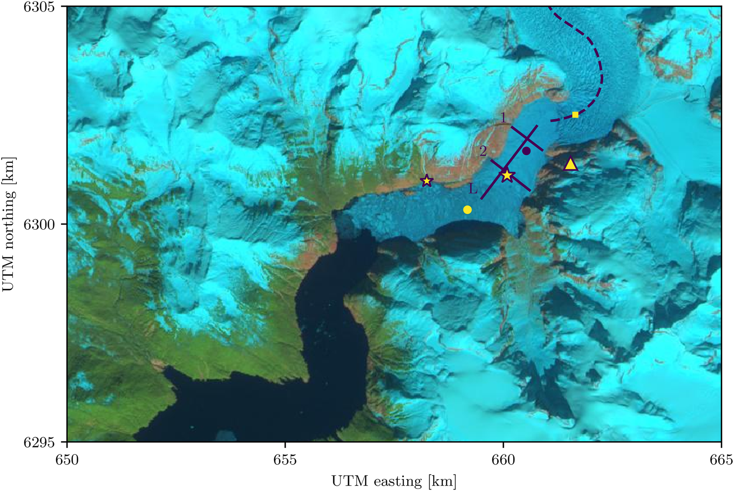
Sentinel-2 image of LeConte Glacier and Bay (UTM zone 8), acquired on 11 April 2017, shortly before the ice mélange began to break apart. The triangle indicates the location of the time-lapse cameras, the meteorological station and the terrestrial radar, and the small and large stars indicate the locations of the land-tethered and deep moorings, respectively. Velocity profiles in Figure 6 are plotted along profiles 1, 2 and L. Changes in terminus position (Figs 2a and 9d) were determined by finding the intersection of the terminus with the glacier centerline (dashed line). The small yellow box corresponds to the same region in Figure 9 over which mean glacier velocities were derived. The ice mélange velocities plotted during break-up in Figure 8 correspond to the locations indicated by the colored circles.
From 2016 to 2017, we instrumented the glacier–fjord system with time-lapse cameras, meteorological stations and moorings, and also measured glacier surface melt during the summer seasons. In addition, we conducted several intensive surveys in which we measured fjord heat, salt and mass fluxes, surveyed the glacier terminus with multibeam sonar, sampled near-terminus waters with remote-controlled kayaks and operated a terrestrial radar interferometer (Kienholz and others, Reference Kienholz2019; Sutherland and others, Reference Sutherland2019; Jackson and others, Reference Jackson2020). This paper focuses on the time series data that were collected during the course of the project and captured the ephemeral ice mélange that was present in the fjord from February to April 2017. Much of the data and methods have been discussed previously; here we describe the key features of the data and methods but refer the reader to Kienholz and others (Reference Kienholz2019) and Sutherland and others (Reference Sutherland2019) for further details. Also, we note that all data were recorded (and are presented here) in Coordinate Universal Time (UTC). Alaska Standard Time is UTC-9:00.
2.1. Time-lapse photography
We operated several time-lapse cameras from a bedrock site adjacent to the glacier. Up to five cameras took photos of the proglacial fjord at high rates (time-lapse intervals of 15 s to 2 min from 6 to 12 h per day, depending on the time of year) (Kienholz and others, Reference Kienholz2019). An additional camera took photos of the lower glacier every hour. The time-lapse systems consisted of Canon Rebel T3, Rebel T5 or EOS 50D single lens reflex cameras. We surveyed the camera locations with a geodetic quality GPS (Trimble NetRS) and measured rotation angles to provide initial estimates for camera model calibration. The time-lapse photos from these cameras allow us to quantify ice mélange velocities, glacier velocities and the glacier terminus position.
2.1.1. Camera calibration
Projection from image coordinates to map coordinates requires a mathematical camera model and a digital elevation model (DEM). We used a camera model with a minimal number of free parameters (Krimmel and Rasmussen, Reference Krimmel and Rasmussen1986). To constrain the camera parameters (yaw, pitch, roll and focal length), we manually digitized the waterline on a WorldView-3 satellite orthoimage from 10 April 2016 (© Digital Globe, Inc., 2016) and on representative time-lapse photos for which the tide was similar to the tide level at the time of the WorldView-3 image. The pixel locations of the waterline in the time-lapse photos were projected into map view using the known camera locations and tidal stage and estimated angles and focal lengths. We then used a least-squares minimization procedure to minimize the distance between the waterline and the projected waterline. Root-mean square errors varied from 5 to 20 m, with larger values down fjord where the look angle was more oblique.
When tracking iceberg motion, we assumed that the features that we were tracking were along a horizontal plane (the fjord surface) that varied in elevation with the tides; in LeConte Bay the tidal amplitude can exceed 6 m during spring tides. For the glacier velocities, we projected pixel coordinates onto a WorldView-2 DEM that was built from images acquired on 23 June 2017 (Porter and others, Reference Porter2018). We shifted the DEM by ±10 m in order to estimate the sensitivity of the projection to errors in the DEM and to changes in glacier surface elevation, which varies seasonally due to surface ablation and dynamic thinning/thickening associated with terminus retreat/advance.
Due to the oblique camera views, the pixel resolution of the imagery differs in the horizontal and vertical dimension and also across the photos. Along the fjord surface, a pixel covers 1.3 m × 17.7 m at a distance of 5.5 km from the cameras but just 0.17 m × 0.34 m at a distance of 700 m. Thus the accuracy of the feature tracking and terminus digitization decreases with distance from the cameras.
2.1.2. Ice mélange and glacier velocities
We determined ice mélange and glacier velocities by applying particle image velocimetry (PIV), as implemented in the Python openPIV module (Taylor and others, Reference Taylor, Gurka, Kopp and Liberzon2010), to successive daily images acquired near solar noon. The images were first filtered with a Gaussian highpass filter with a five-pixel standard deviation in order to enhance high contrast edges (see also Fahnestock and others, Reference Fahnestock2016). We used a correlation window size of 128 pixels by 128 pixels with 75% overlap (i.e., the distance between the centers of adjacent windows was 32 pixels). All correlations with a signal-to-noise ratio less than 1.2 were excluded because the associated velocity vectors were often inconsistent with adjacent windows (in magnitude and/or direction).
The glacier and iceberg velocities were averaged over 100 m by 100 m squares. The standard deviation of the velocities within these squares provides an estimate of the uncertainty. For the yellow square shown in Figure 1, the standard deviation varied seasonally and ranged from 1–4 m d−1. The standard deviation was lowest in the spring and summer of both years and highest in fall 2016. Some of the variance in calculated velocities is due to spatial variations in velocity. For example, longitudinal strain rates near the glacier terminus are on the order of 0.015 d−1 (O'Neel and others, Reference O'Neel, Echelmeyer and Motyka2001; Sutherland and others, Reference Sutherland2019), which results in the velocity varying by 1.5 m d−1 across the length of the square. In contrast, the seasonal variations in the standard deviation are likely related to seasonal retreat and thinning, which resulted in large differences between the DEM and the true surface elevation, especially when the terminus was in a retreated position. Shifting the DEM vertically by ±10 m typically changed the velocity by 1–2 m d−1. In addition, when the terminus was in a retreated position, the distance from the sampling region to the terminus became small. The high flow speeds near the terminus are associated with serac falls and avalanches, which changes the surface texture between images and increases the perceived flow variability. Taken together, we assume the uncertainty in our PIV-derived velocity calculations to be ~2 m d−1.
During ice mélange break-up, the icebergs moved too quickly to be tracked across daily images. Instead of changing our sampling strategy, we instead rely on the results of Kienholz and others (Reference Kienholz2019), who applied sparse optical flow to track icebergs over short time periods (15–120 s) and used the iceberg velocity fields as proxies for fjord surface currents. Although the workflow was designed to track freely flowing icebergs, it also works well in other applications as long as changes in illumination between successive images are small (i.e., the time-lapse interval is small). In our workflow, we detect iceberg corners with the Shi-Tomasi algorithm (Shi and Tomasi, Reference Shi and Tomasi1994) and track the motion of these corners across several images with the Lucas–Kanade algorithm (Lucas and Kanade, Reference Lucas and Kanade1981). Both algorithms are implemented in openCV (https://opencv.org). The calculated velocities were gridded and averaged over 30 min, non-overlapping windows.
2.1.3. Glacier terminus position
The glacier terminus position was determined by manually digitizing the top of the terminus in daily images. We chose to digitize the top of the terminus instead of the more clearly delineated waterline, as used in some previous studies (e.g., Otero and others, Reference Otero2017), because our cameras did not always provide us with a clear view of the entire waterline. The terminus elevation varies temporally and seasonally. We assumed a constant elevation of 50 m, but tested the effect of shifting the elevation by ±20 m, which results in an apparent and systematic shift in the terminus position by ~25 m horizontally (larger than but of similar magnitude to the uncertainty in digitizing the waterline; see discussion above). After projecting pixel coordinates into map view, we determined the intersection of the terminus with the glacier centerline (Kienholz and others, Reference Kienholz, Rich, Arendt and Hock2014), which we defined as the terminus position. Similar to the choice of using the top of the terminus instead of the waterline, we chose to use the centerline position instead of an average terminus position due to difficulties in delineating the entire terminus in the time-lapse imagery.
2.1.4. Frontal ablation rate
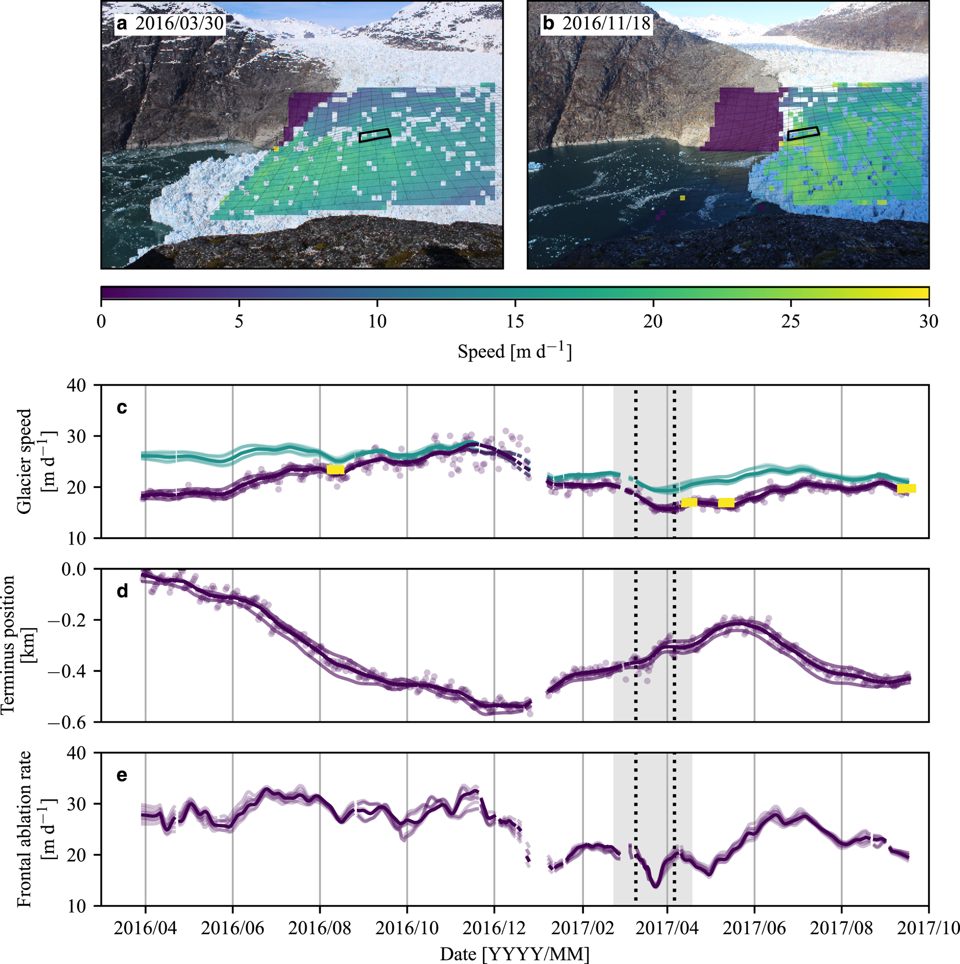
To estimate temporal variations in frontal ablation rates (iceberg calving plus submarine melting), we calculate the frontal ablation rate U f along the glacier centerline as U f = U t − dL/dt, where U t is terminus velocity and L is glacier length. Since PIV generally does not work well near the glacier terminus due to serac falls and calving events, we estimate the terminus velocity by using the velocity at a fixed Eulerian point U 0 (yellow square in Fig. 1) and assuming a constant longitudinal strain rate of $\dot \epsilon _{{\rm L}}=0.015$ d−1. The terminus velocity is then given by $U_{\rm t}=U_0+\dot \epsilon _{{\rm L}}L$
 , where L is the distance from the Eulerian point to the terminus. Prior to calculating the frontal ablation rate, we smoothed the velocity and terminus position time series with a LOWESS (locally weighted scatterplot smoothing) filter with a smoothing span of 28 days. This smoothing was necessary in order to remove variations due to discrete calving events and to reduce noise associated with computing the derivative of the glacier length time series.
2.2. Terrestrial radar data
During four approximately week-long field campaigns, we operated a Gamma Remote Sensing ground portable radar interferometer (GPRI) to measure near-terminus glacier velocities (see Sutherland and others, Reference Sutherland2019). Data from the GPRI provides an important, independent check on glacier velocities derived from our time-lapse imagery. The GPRI is a Ku-band (λ = 1.74 cm) real aperture imaging radar that has a maximum range of 16 km (set to 8 km here), a range resolution of 0.75 m, and an azimuth resolution that is proportional to range. For our area of interest, the azimuth resolution was ~3 m in the near-field and 21 m in the far-field at distances of 0.4 and 3 km, respectively. We programmed the GPRI to scan a 120° swath every 3 min. We reprojected the radar backscatter images into Cartesian space, georectified to UTM zone 8 with the 2012 Alaska Interferometric Synthetic Aperture Radar (IfSAR) DEM (USGS, 2019) as input, and interpolated onto a 10 m resolution grid.
To generate velocity fields from the backscatter images, we again used the Shi-Tomasi algorithm to detect corners and the Lucas–Kanade algorithm to track corners over sliding 12 h windows. The velocity vectors were interpolated onto a 50 m grid and stacked to produce campaign averages.
2.3. Meteorological data and glacier runoff
We collected temperature, precipitation, wind speed and wind direction with a Campbell Scientific weather station located near the time-lapse cameras and terrestrial radar. The temperature and precipitation data were used to drive an Enhanced Temperature Index Model (Hock, Reference Hock1999) coupled to an accumulation model and a linear reservoir-based discharge routing model (e.g., Hock and Noetzli, Reference Hock and Noetzli1997). The model ran at hourly time steps on a 100 × 100 m grid. Data gaps were filled with data from a secondary weather station on the north side of the fjord. To constrain temperature lapse rates and precipitation gradients, we deployed an additional weather station ~6 km up glacier from the terminus on bedrock. For the surface mass-balance model calibration, we relied on sparse mass-balance measurements collected at four mass-balance stations during the 2016 and 2017 seasons. Since the parameters of our model are either loosely constrained (five parameters of the surface mass-balance model) or not constrained by field measurements (four parameters of discharge routing model), we conducted a sensitivity analysis to generate low, middle and high runoff scenarios. The middle scenario comprises the mass-balance model parameter combination that minimizes the difference between modeled mass balances and measured in situ surface mass balances in the root-mean-square-error sense. All model variables were held constant over time. For more details, see Sutherland and others (Reference Sutherland2019).
2.4. Mooring data
We deployed a deep mooring in LeConte Bay in March 2016, serviced and redeployed it in August 2016 and May 2017, and ultimately retrieved it in September 2017. Its location from August 2016 to September 2017 is indicated in Figure 1; prior to that it was located ~1 km farther down fjord. The mooring contained over ten instruments. In this study, we are primarily concerned with comparing bulk changes in fjord water properties to the formation and break-up of ice mélange. For clarity, we therefore only plot data from a few instruments: three conductivity, temperature and depth sensors (CTDs; Seabird MicroCAT SBE37s) and an upward looking 300 kHz Acoustic Doppler Current Profiler (ADCP; RDI Workhorse). The CTDs were deployed at depths of ~110, 170, and 190 m; the depths varied across deployments by ~15 m. The instruments recorded pressure, temperature and salinity every 3 min; the data were later interpolated to 15 min and filtered to remove data points that differed from the running mean by more than five standard deviations. Note that the salinity measurements for the instrument at 110 m depth were erratic from 25 December 2016 to 8 May 2017 and were therefore excluded. The upward-facing ADCP was deployed at 106 m depth and measured velocity in 4 m bins from 12 to 96 m depth. The velocities in the upper 12 m were discarded due to side lobe contamination from the surface. The ADCP pings (at 40 s intervals) were averaged over 60 min, and the resultant velocities were rotated into along- and across-fjord components and smoothed with a LOWESS filter (using a 7-day smoothing span) in order to highlight long-term fluctuations in velocity.
In addition to the deep mooring, we also deployed a shallow land-tethered mooring on the north side of the fjord (Fig. 1). This mooring contained four instruments; we only plot data from a RBRsoloT temperature logger that was deployed to a depth of 30 m. It recorded data every 3 min, which was later interpolated to 15 min. Note that, unlike the ADCP measurements, we did not apply any additional filtering to the temperature or salinity measurements from either mooring, since the magnitude of short-term fluctuations in these properties provide a qualitative assessment of fjord stratification, with the fjord being most stratified when the fluctuations have high amplitude.
3. Results
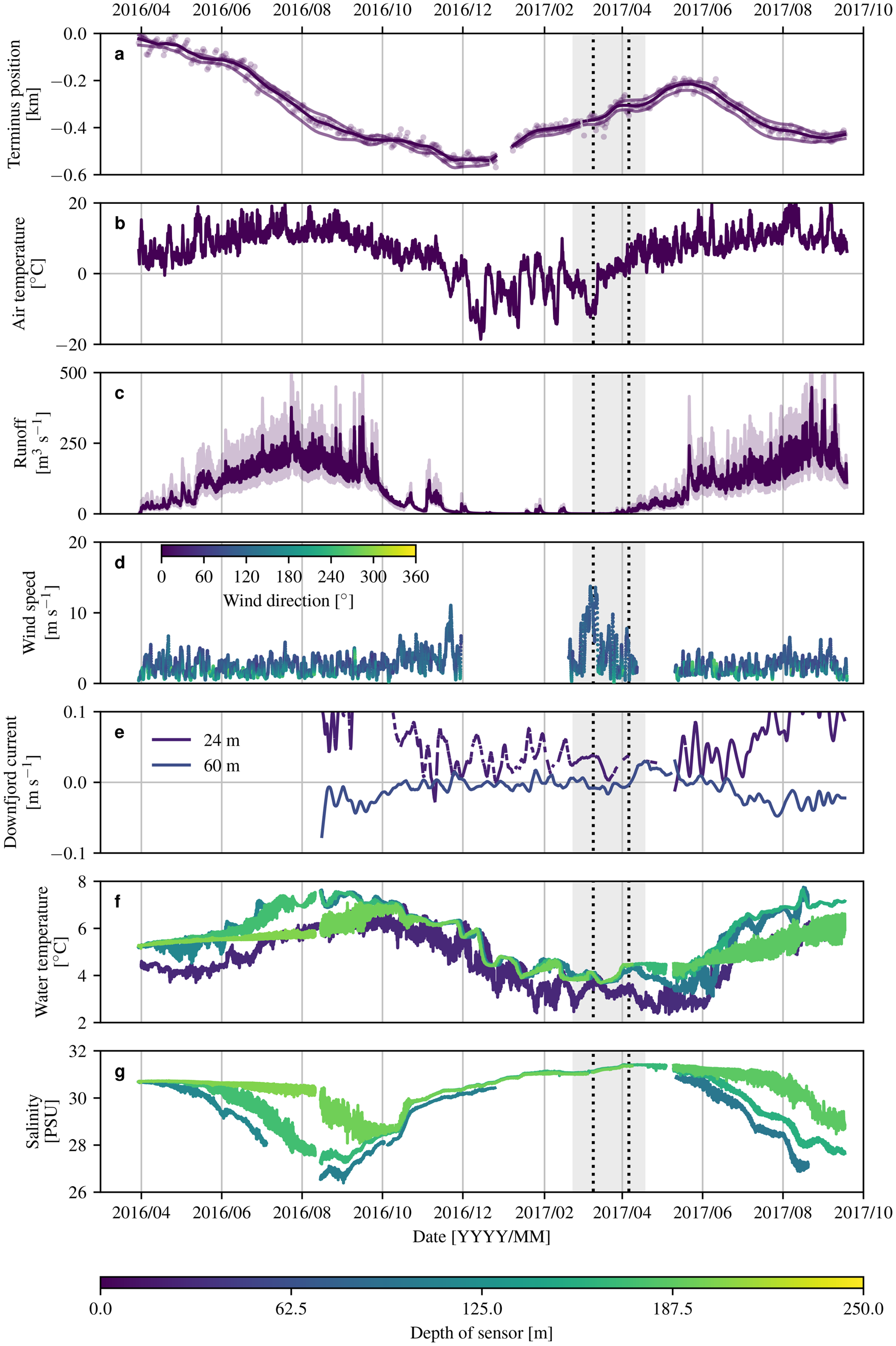
The development of a thick, cohesive ice mélange in LeConte Bay occurred after sea ice formed in February 2017. Our time-lapse imagery indicates that sea ice had formed overnight on a couple of prior occasions that winter, but it was not until 22 February that the sea ice persisted for multiple days. This persistent sea ice coverage formed about 2.5 months after air temperatures dropped below 0°C, water temperatures dropped from their summer maximum of 5–7°C down to 1–4°C, and fjord stratification weakened significantly (as indicated by reduced temperature and salinity variations with depth and diminished tidal fluctuations in temperature and salinity) (Fig. 2). The sea ice and nascent ice mélange were sufficiently strong to withstand the strongest down fjord winds that we observed (sustained winds in excess of 10 m s−1 for several days), which occurred about a week after the fjord became ice covered (Fig. 2d).
Time series of (a) relative terminus position (with uncertainty due to assumed terminus elevation), (b) air temperature, (c) estimated subglacial discharge (light purple indicates sensitivity of discharge calculations), (d) wind speed and direction and (e)–(g) down fjord currents, temperature and salinity from mooring data. The gray-shaded regions in all panels indicate when the ice mélange was present. The vertical dashed lines bracket the period of quasi-static flow (e.g., see Figs 5c,d).
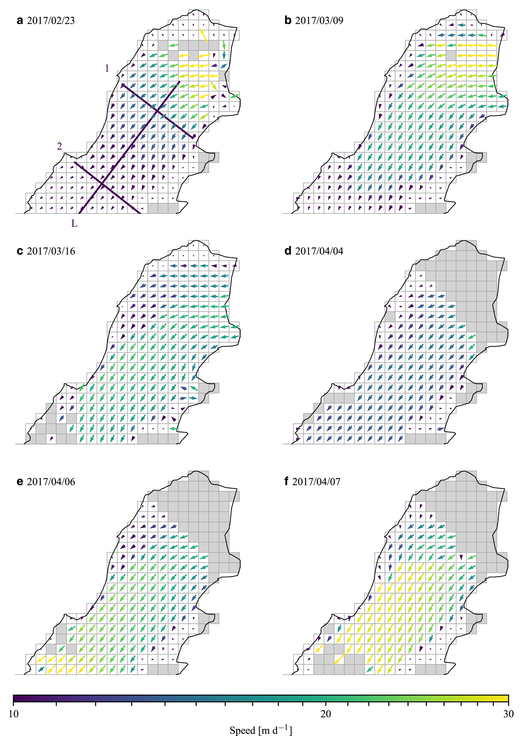
Immediately following sea ice formation, the fjord surface was smooth and icebergs were widely dispersed (Figs 3 and 4). As the glacier terminus continued its winter advance and occasionally calved icebergs, the iceberg packing fraction increased and the fjord surface became increasingly similar to ice mélange found in Greenland, such that by mid-March it became difficult to delineate the glacier–ice mélange boundary.
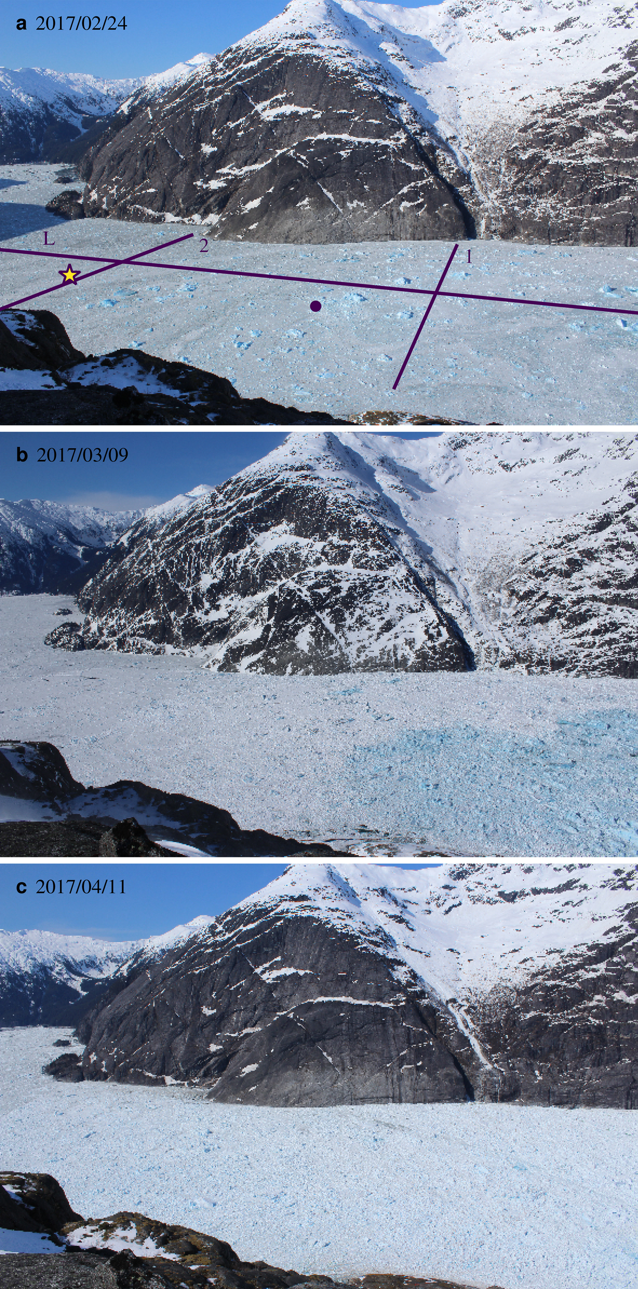
Time-lapse photos illustrating the change in appearance of the fjord as sea ice was compacted into ice mélange via terminus advance and occasional calving events. As in Figure 1, the star, yellow lines and circle indicate the locations of the mooring, the transects that are plotted in Figure 6, and one of the points that corresponds to the velocity time series in Figure 8, respectively.
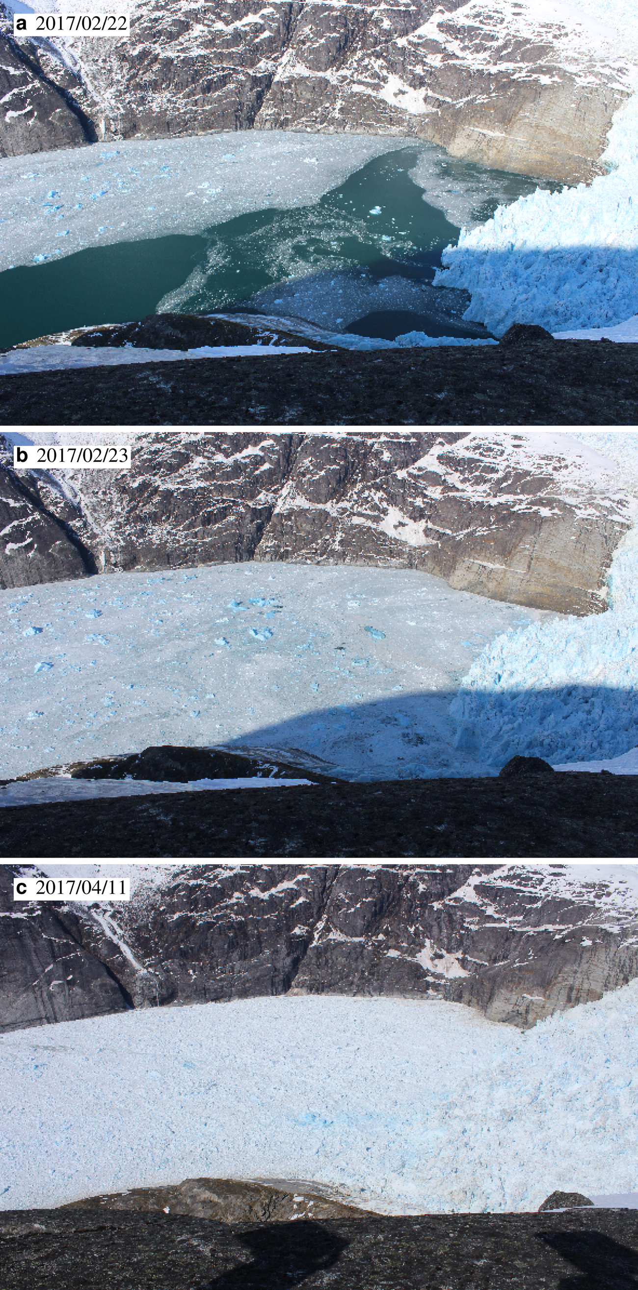
Time-lapse photos illustrating the change in appearance of the glacier terminus as sea ice formed and was compacted into ice mélange.
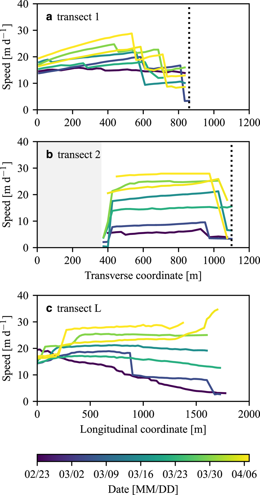
The transition in fjord appearance coincided with a transition in flow. Initially, the ice flow in the fjord was highly compressive and shear strain rates were minimal (Figs 5a,b and 6). As the iceberg packing fraction increased, the flow became increasingly uniform in the longitudinal direction (Figs 5c,d and 6) and velocities generally increased in time. Deformation was concentrated in narrow shear bands along the fjord margins and within the ice mélange, although shear strain also occurred across the ice mélange. Shear strain rates were largest close to the glacier terminus and appear to have gradually increased with time (Figs 6a,b).
Average daily ice mélange velocity fields illustrating (a)–(b) compressional flow, (c)–(d) quasi-static flow and (e)–(f) extensional flow. Note the logarithmic color scale. The boxes are 100 m on a side.
(a)–(b) Transverse (north is to the right) and (c) longitudinal velocity profiles of the ice mélange. The profiles correspond to transects 1, 2 and L in Figure 1, respectively. The dotted lines indicate the ends of the transects, and the gray-shaded region in (b) corresponds to a small embayment that was out of view of the cameras.
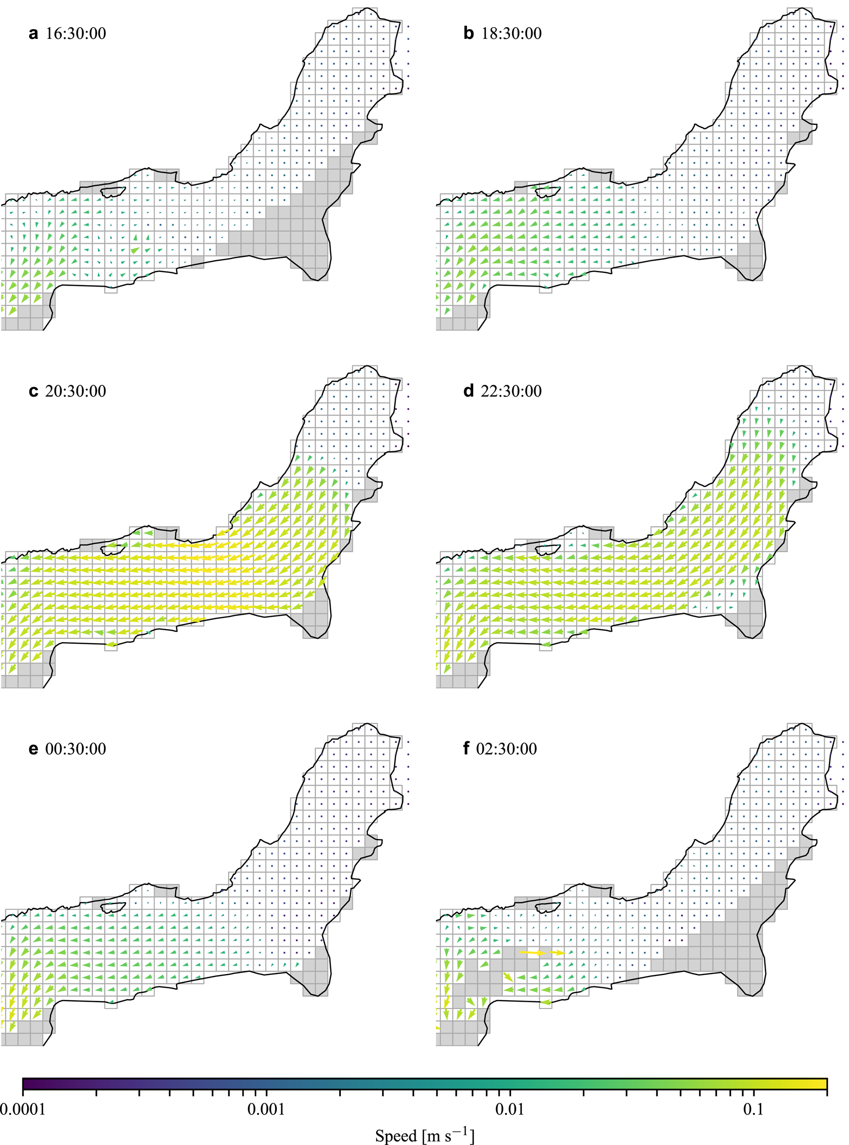
After about a month of quasi-static flow, the ice mélange began to experience extensional flow in early April (Figs 5e,f and 6), coincident with a rise in air temperatures, onset of glacier runoff and increased down fjord currents at depths ≥ 60 m, and increasing fjord stratification at greater depths (Fig. 2). Break-up of the ice mélange began in earnest on 11 April (local time) and occurred over a period of 6 days (Figs 7 and 8). The break-up was episodic. Each day, the ice mélange experienced pulses of rapid flow in excess of 0.1 m s−1 for a few hours (several hundred times faster than the quasi-static flow that preceded break-up) and then rapidly slowed to pre-break-up velocities (Video S1). The upwelling meltwater plume became visible at the fjord surface as the ice mélange finished disintegrating (Video S2).
Ice mélange velocity fields on 12 April 2017, during the ice mélange break-up, derived from the Lucas–Kanade optical flow method (Kienholz and others, Reference Kienholz2019). Note the logarithmic color scale. High velocities only occurred for a few hours in the middle of the day. The boxes are 100 m on a side.
Time series of (a) iceberg velocities derived from the Lucas–Kanade method, overlain by tidal stage, and (b) glacier runoff and associated uncertainties (as in Fig. 2c). In (a), the colored dots correspond to the locations shown in Figure 1, where purple is up fjord and yellow is down fjord. The annotations indicate (i) periods in which fast flow was clearly linked to energy released by calving icebergs (‘intensive calving’ and ‘calving event’), (ii) a period of fast flow in which no calving events occurred (‘no calving’), and (iii) the emergence of the plume at the fjord surface and ultimate disintegration of the ice mélange (‘final break-up’).
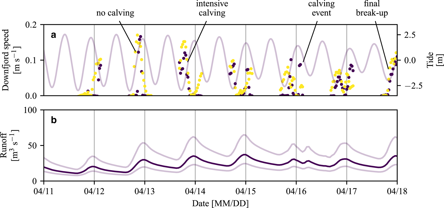
The patterns of rapid flow varied during each of these pulses. Some pulses originated down fjord, propagated toward the glacier terminus (see Video S1), and were loosely correlated with the outgoing tide and/or glacier runoff. These pulses are clearest for events that originated around 00:00 and 20:00 on 12 April (Fig. 8; note the lag between the yellow and purple dots). During these pulses the boundary of visually thick ice mélange propagated up fjord in discrete steps (Video S1), similar to the observations of Xie and others (Reference Xie, Dixon, Holland, Voytenko and Vaňková2019). Other periods of rapid motion were caused or amplified by the energy released by calving icebergs. For example, rapid motion that occurred early on 13 April was associated with vigorous calving activity, and the event that occurred at 00:30 on 16 April can be entirely attributed to a calving iceberg (Video S1) and appears similar to dynamic jamming events that have been observed in ice mélange in Greenland (Peters and others, Reference Peters2015). Calving events that occurred when the ice mélange was more rigid did not produce such sustained and expansive increases in flow.
The lowest glacier velocities that we observed, which were ~19 m d−1, occurred when the ice mélange was in place (Fig. 9). Since the glacier advanced at a steady rate of ~2 m d−1 throughout the winter (and up to 4–5 m d−1), the lowest frontal ablation rates also occurred at this time yet still exceeded 14 m d−1. Unlike some observations from Greenland (e.g., Cassotto and others, Reference Cassotto, Fahnestock, Amundson, Truffer and Joughin2015; Motyka and others, Reference Motyka2017; Amundson and Burton, Reference Amundson and Burton2018; Xie and others, Reference Xie, Dixon, Holland, Voytenko and Vaňková2019), the onset of summer terminus retreat did not coincide with the ice mélange disintegration. However, on several days during the week-long break-up, calving occurred shortly after the region of rapidly flowing ice mélange approached the terminus (Video S1).
(a)–(b) Example glacier velocity fields derived from time-lapse photogrammetry. (c) Glacier velocity time series, where purple is the average velocity in the black square in panels (a) and (b) and blue is the estimated terminus velocity. Average campaign velocities derived independently from terrestrial radar data are indicated by yellow boxes (Sutherland and others, Reference Sutherland2019), which agree with and serve to validate the lengthier, time-lapse derived velocity time series. (d) Relative terminus position (repeated from Fig. 2a for comparison purposes). (e) Frontal ablation rate along the glacier centerline. The dark curves in (c)–(e) are computed by applying a LOWESS filter to the velocity and terminus position time series derived from the 23 June 2017 DEM and assuming a constant terminus elevation of 50 m. The light curves represent the LOWESS filtered data when the DEM is shifted by ±10 m and the assumed terminus elevation is shifted by ±20 m. The gray-shaded regions in panels (c)–(d) indicate when the ice mélange was present. The vertical dashed lines bracket the period of quasi-static ice mélange flow.
4. Interpretation
Although ice mélange is relatively rare in Alaska, its formation is not unprecedented (Fig. 44 in Molnia, Reference Molnia2008; Welty and others, Reference Welty, O'Neel, Pfeffer, Balog and LeWinter2012; McNabb and Hock, Reference McNabb and Hock2014). Inspection of Landsat imagery indicates that ice mélange formed in LeConte Bay at least once during the past decade, in February 2011. Persistent cloud cover in the region may have obscured its occurrence in other years. In 2017, ice mélange persisted in LeConte Bay for about 2 months. It formed after extended periods of cold air and water temperatures, and during a time that glacier runoff was minimal. Once the ice mélange formed, down fjord winds appear to have had very little impact on its behavior. Extension and then break-up of the ice mélange coincided with warming air temperatures, the onset of glacier runoff and the resulting development of a weak plume (as indicated by outflow over the uppermost 60 m of the water column and increasing fjord stratification at depth). Additionally, once break-up had initiated, outgoing tides helped to pull the ice mélange apart during the day (Fig. 8). At night, lower air temperatures and decreased plume activity may have promoted sea ice growth sufficiently to prevent ice mélange expansion.
The ice mélange velocity fields that we observed are generally consistent with viscoplastic rheologies that have been proposed for granular materials, which are based on experiments that exhibit viscous deformation at high pressures and block flow at low pressures (e.g., Jop and others, Reference Jop, Forterre and Poulique2006; Henann and Kamrin, Reference Henann and Kamrin2013, Reference Henann and Kamrin2014). Ice mélange develops a wedge as it is compacted (Amundson and Burton, Reference Amundson and Burton2018; Xie and others, Reference Xie, Dixon, Holland, Voytenko and Vaňková2019), and consequently the pressure is high near the glacier terminus and decreases in the down fjord direction. Transverse velocity profiles should therefore exhibit viscous deformation near the terminus and block flow down fjord (Amundson and Burton, Reference Amundson and Burton2018), consistent with our observation of higher shear strain rates across transect 1 (Fig. 6a) than across transect 2 (Fig. 6b). Other aspects of ice mélange flow, such as shear bands within the ice mélange and large fluctuations in velocity during break-up, are more difficult to reconcile with previous theoretical work, which has generally assumed idealized fjord geometries and not accounted for short timescale (i.e., diurnal) variations in rheology due to growth and decay of sea ice.
The lowest glacier velocities and frontal ablation rates occurred when the ice mélange was most extensive and highly compacted. However, it is difficult to determine cause and effect. The glacier steadily advanced during the winter from December through mid-May, with only small changes in the rate of advance associated with ice mélange formation or break-up. Theoretical work suggests that ice mélange may be sufficiently strong to inhibit calving (at least for full-glacier-thickness calving events in Greenland) when the ice mélange length-to-width ratio is greater than ~3 (Amundson and others, Reference Amundson2010; Burton and others, Reference Burton, Amundson, Cassotto, Kuo and Dennin2018; Amundson and Burton, Reference Amundson and Burton2018). At its peak extent, the ice mélange in LeConte Bay was ~3 km long and, since the fjord is ~1 km wide, its length-to-width ratio was ~3. Thus the ice mélange that we observed may have just been at the threshold of being able to prevent calving events from occurring and may have simply required more time to thicken and lengthen before it had a clear impact on iceberg calving. Additionally, the sinuous geometry of the lower glacier may result in a situation where lateral shear stresses dominate over longitudinal stresses, and therefore changes in resistive stresses from ice mélange may have relatively little impact on glacier dynamics. Future studies should attempt to address the relationship between glacier sinuosity and terminus stress balance, as this may explain why some glaciers appear to be more sensitive to changes in ice mélange formation and break-up than others.
5. A systems perspective of ice mélange
Over the past couple of decades, tidewater glaciers worldwide have been experiencing rapid changes in flow and geometry that are strongly influenced by processes occurring at the glacier–ocean boundary. Numerous studies have targeted these processes in an effort to improve projections of glacier and ice-sheet evolution and associated sea level rise. A comprehensive picture is emerging of the couplings between subglacial discharge, plume dynamics, fjord circulation and submarine melting (e.g., Carroll and others, Reference Carroll2015) and the impacts that submarine melting, iceberg calving and surface melting have on tidewater glacier dynamics (e.g., Cowton and others, Reference Cowton, Todd and Benn2019). In contrast, ice mélange and other fjord ice coverage (sea ice and freely floating icebergs) have not yet been fully integrated into the glacier–ocean system. In Figure 10, we indicate what we feel are the key couplings affecting ice mélange behavior (Roman numerals in the following paragraphs correspond to processes indicated in the figure).
Schematic of the glacier–ocean–mélange system that illustrates the important mechanical and thermodynamic couplings that affect the mechanical properties of ice mélange. Many of these system couplings are poorly constrained.
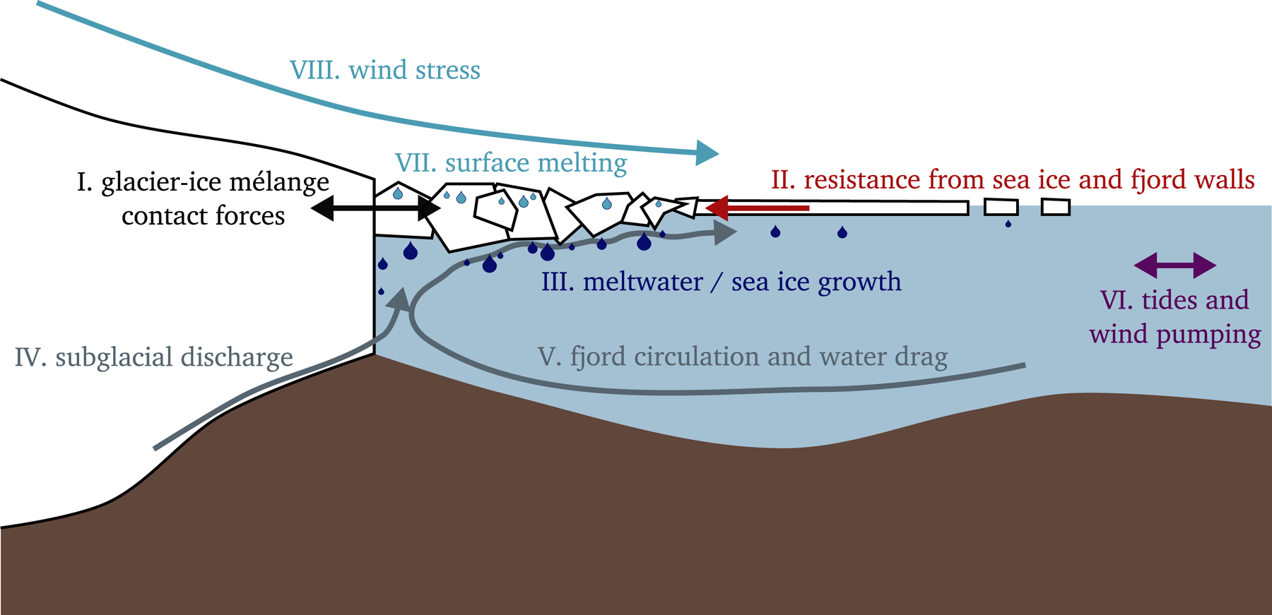
Some attempts have been made to quantify the transfer of resistive stresses from fjord walls to glacier termini (I and II) (Amundson and others, Reference Amundson2010; Burton and others, Reference Burton, Amundson, Cassotto, Kuo and Dennin2018; Amundson and Burton, Reference Amundson and Burton2018) and the impact of calving events on ice mélange flow (I) (Peters and others, Reference Peters2015). Building on observations that suggest that ice mélange can affect glacier terminus dynamics, a few studies have used ad-hoc parameterizations of ice mélange in tidewater glacier models (Pollard and others, Reference Pollard, DeConto and Alley2018; Todd and others, Reference Todd, Christofferson, Zwinger, Råback and Benn2019). In parallel to this work, recent observations have quantified meltwater fluxes from icebergs and ice mélange (III) (Enderlin and others, Reference Enderlin, Hamilton, Straneo and Sutherland2016; Moon and others, Reference Moon2018), and related changes in water temperatures to ice mélange rigidity and glacier dynamics (III) (Bevan and others, Reference Bevan, Luckman, Benn, Cowton and Todd2019; Joughin and others, Reference Joughin, Shean, Smith and Floricioiu2020). To date, however, no study has systematically addressed the couplings and feedbacks between the various components of the glacier–ocean–ice mélange system.
Couplings between ice mélange and the ocean, which include both thermodynamic and mechanical couplings, are particularly poorly understood. Ice mélange injects cold freshwater into fjords near glacier termini that, in conjunction with subglacial discharge (IV), affects fjord buoyancy, heat transport (V) and submarine melting of icebergs. In some regards, the situation is similar to submarine melting of ice shelves. However, an important distinction is that ice mélange has an extremely rough underside, with a disproportionately large surface area compared to ice shelves, and can inject freshwater across a range of depths. The rough topography also imparts drag forces on the underlying water and forces near-surface currents to follow complex pathways (V). Thus, the ice mélange topography affects the ability of the outflowing plume and other currents to melt icebergs (since plume theory indicates that melt rates scale with water velocity; e.g., Jenkins, Reference Jenkins2011; Jackson and others, Reference Jackson2020), and to pull icebergs apart from each other. Our observations suggest that tides (VI), the outflowing plume (V), melting of icebergs (III and VII) and calving events (I) work together to cause the break-up and dispersal of ice mélange. These processes must therefore all affect the mechanical properties of ice mélange and its ability to influence tidewater glacier stability. In contrast, our observations indicate that strong down fjord winds (VIII) have relatively little impact on the mechanical properties of ice mélange.
Improving our understanding of the role of ice mélange in the glacier–ocean system requires us to confront the complex interactions between ice mélange, fjord circulation and glacier dynamics. Given the difficulty of observing ice mélange processes in the field, it will likely be necessary to draw heavily on modeling studies designed to test the sensitivity of ice mélange flow and stress to these various couplings.
6. Conclusions
We observed the formation, flow and break-up of ice mélange at LeConte Glacier and Bay, the southernmost tidewater glacier system in the Northern Hemisphere. Our observations highlight the challenges of trying to understand and model the impacts of ice mélange on glacier–fjord systems, in particular because many aspects of these systems are affected by the same forcings. For example, we observed low glacier velocities and frontal ablation rates when ice mélange was present and flowing quasi-statically. Resistance from ice mélange may have directly (or indirectly) impacted glacier flow, but alternatively low velocities and calving rates could have simply resulted from the lack of water input to the glacier bed or seasonal terminus advance that increased basal and lateral shear stresses. Similarly, ice mélange break-up was well correlated with increased glacier runoff and the development of a subsurface plume, which may have helped to drive icebergs down the fjord and eroded the underside of the ice mélange. However, ice mélange may also have simply reached a weakened state due to surface melting of sea ice and icebergs, the same process that drove the increase in glacier runoff. Disentangling these couplings and feedbacks between ice mélange, glacier dynamics and fjord processes will require comprehensive, systems-based field and modeling studies.
Supplementary material
The supplementary material for this article can be found at https://doi.org/10.1017/jog.2020.29
Acknowledgments
This work was supported by the US NSF awards OPP-1503910, OPP-1504191, OPP-1504288, OPP-1504521 and DMR-1506307.
The WorldView imagery and DEM were provided by the Polar Geospatial Center under US NSF awards OPP-1043681, OPP-1559691 and OPP-1542736. The IfSAR DEM is distributed through the USGS Earth Resources Observation Center. Field logistics was provided by CH2MHill Polar Field Services and would not have been possible without the help of the crew of the MV Steller and MV Pelican, Temsco Helicopters, Petersburg High School and the US Forest Service. We also thank J.B. Mickett, D.S. Winters, W.P. Dryer, A. Stewart, M. Michels, C. Carr, T. Moon, A. Simpson and E.C. Pettit for assistance with field work and data processing and M. Truffer for loaning the GPRI radar interferometer.


 Open access