That’s why I’ve written this book.

Let’s take it one step at a time. The dialogue above introduces most of the steps in making good decisions using language that is familiar. But what are the ingredients? There are just 10 ingredients, which we will discover by working through a hypothetical problem, and along the way I’ll show how to combine the ingredients using ‘logical glue’, the term coined by Howard Raiffa in his ground-breaking 1968 book, Decision Analysis.¹ Once the ingredients and logical glue are made clear, you will be prepared for the framework, which I’ll present at the end of the chapter. That framework will provide you with the ability to take a fresh look at any decision.

The Blind Problem

We start with a simple decision, for if we can understand how decision theory works for a simple problem, we are more likely to apply it correctly for real small-world decisions. Imagine that you have been suffering difficulty seeing clearly and your optician suggests you consult an ophthalmologist. After a careful examination, she tells you that you have a rare eye disease, which if left untreated, will cause you to become permanently blind in both eyes. However, an operation could restore your full sight, but that is not guaranteed as it is a new treatment and is not always successful, in which case the operation will leave you … dead.

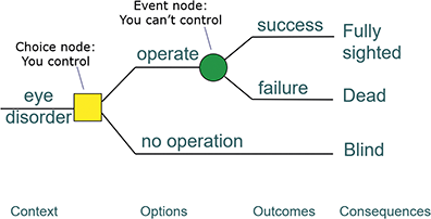
At this point, most people would ask questions to see if other alternatives would reduce the risk, but let’s stay with this example because it is perhaps the simplest sort of choice under uncertainty, an uncertain event compared to a certainty, and it easily portrays elements of the vocabulary you will need to make sense of many difficult problems. Figure 1.1 shows a simple decision tree of the eye problem.

Figure 1.1

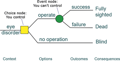
Figure 1.1 Long description

The context is an eye disorder. This leads to the first node, labelled Choice node: You control, which branches into two options: operate and no operation (which leads to the consequence Blind). Operate leads to the next node, labelled Event node: You can’t control, which branches to two outcomes: success (leading to the consequence Fully sighted), and failure (leading to the consequence Dead).

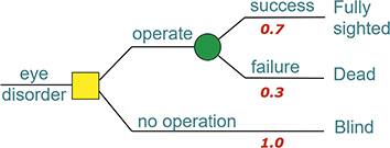
What more would you like to know? Most people to whom I’ve posed this problem ask what the chance of success is. The ophthalmologist says about 70 per cent. I will discuss probabilities in Chapter 6, and we will examine the basis for assigning a probability. For now, assume 70 per cent, shown properly on a decision tree as decimal numbers between 0 and 1.0, inclusive (Figure 1.2).

Figure 1.2

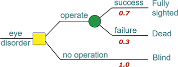
Figure 1.2 Long description

The context is an eye disorder, which leads to two branches: operate and no operation. No operation has a p-value of 1.0, and leads to Blind. Operate branches into two paths: success (p-value of 0.7; leads to Fully sighted) and failure (p-value of 0.3; leads to Dead).

For now, consider what you think you would do. Agree to the operation with a 70 per cent chance of success leading to your sight restored and a 30 per cent chance of dying on the operating table, OR reject the operation and go blind in both eyes within the next three months?

Now, set aside your choice and let’s work through the problem. I presume that you would prefer to be fully sighted rather than blind, and you would prefer being blind in both eyes to being dead. Two simple comparisons which lead me to suppose you therefore prefer being fully sighted to being dead. If so, then your order of preference would be fully sighted, blind, dead. What you probably didn’t say was, ‘I don’t know’ for one of the comparisons, although some people do and tell me they would have to think more deeply about it.

You might have asked, ‘What do you mean by “preference”?’ The Oxford Dictionary definition – ‘liking of one thing better than another’ – will do, and in plain English means desirability, worth or value. In other words, it’s the preference for a consequence regardless of its probability, a preference value. We’ll now analyse the problem further to construct your preferences between the options.

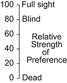
Let’s start by assigning a pair of arbitrary numbers to represent the preference value to you of the two extreme consequences: 100 to fully sighted and 0 to dead. Relative to those two numbers, what would you assign to being blind? Is it closer to 100 or to 0? If you say ‘50’, then I would ask, ‘Since 50 is halfway between 100, then does it follow for you that being fully sighted is as much better than being blind as being dead is worse?’

This is a comparison of preference values based on the added value to you of being fully sighted instead of blind, compared to the added value of being blind rather than dead. Most people say those increments of value are not the same: the dead-to-blind increment is quite a bit larger than the blind-to-fully-sighted increment. If I ask how much bigger, some might say four times bigger, which suggests that blind could be given an 80 since 0 to 80 is four times the 20-point difference between blind and fully sighted (Figure 1.3).

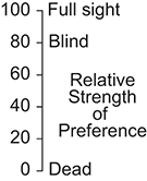
As I’m sure you appreciate, there is no correct answer here; the number you assign depends on many things that are personal to you, so others might assess different numbers for themselves. The context of the decision is crucial, for it will influence this assessment and all those to follow. Let’s proceed with the 80. All the consequences are now located on a 0–100 preference value scale whose numbers represent your relative strengths of preference for the consequences.

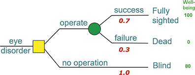
The updated decision tree is shown in Figure 1.4. Is it possible to place the decisions on the 0–100 preference value scale? Since ‘don’t operate’ leads to certain blindness, which was scored at 80, that number also represents the relative value of the decision. But ‘operate’ could lead to either of two differently valued consequences, so how can a single number represent the preference value of that decision?

Figure 1.4

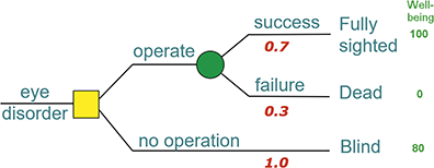
Figure 1.4 Long description

The context is an eye disorder, which leads to two branches: operate and no operation. No operation has a p-value of 1.0, and leads to Blind (well-being is 90). Operate branches into two paths: success (p-value of 0.7; leads to Fully sighted; well-being is 100) and failure (p-value of 0.3; leads to Dead; well-being is 0).

Certainty Equivalents

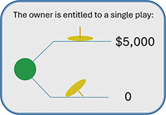
Let’s see how we can find that single number. Imagine I gave you the ticket shown in Figure 1.5.

You now own it. A third person will toss the thumbtack (drawing pin in the UK) onto a hard tabletop, where it will land either with its point up or down. If it lands point up, I give you $5,000, but if it lands point down, nothing. Before the toss, you can examine the thumbtack, which I randomly selected from a package of them from a stationer’s store, but you aren’t allowed to gather data by tossing it many times. I think you would agree this a good deal. You don’t have to pay for the toss, so you might be better off by $5,000, but no money lost if point down is the outcome.

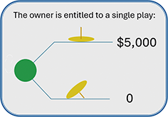
If for any reason you wouldn’t like to play this gamble, you might consider selling it. What would you consider to be a fair selling price? If the chances of the two outcomes were equal, then you would have a 0.5 chance of winning $5,000 and 0.5 of winning nothing. So, it’s clear that, at best, the monetary value of the gamble might be $2,500, which is £5,000 times 0.5. ‘Yes,’ you say, ‘If someone offered me $2,500, I would take it.’ Let’s define that as the certain monetary equivalent. It’s the single certain equivalent that you judge would be fair. And if you are pretty sure the probability is less than 0.5, say 0.4, then the certain monetary equivalent would be $2,000. In general, the lower the probability of success, the less attractive the wager.

The wager would also be less attractive if there was a penalty for the drawing pin landing pin down. For example, suppose that outcome would cost the owner of the wager $1,000. Multiply that loss by the probability of failure, 0.5 if success is also 0.5, and the weighted monetary value of –$1,000 is –$500. Now, add that to the +$2,500 and the fair value of the wager becomes less attractive at $2,000. This summing of weighted values is referred to as an ‘expected’ value, so the $2,000 is considered as an expected monetary value, or EMV, although you ‘expect’ either $5,000 or nothing. That’s the idea we’ll now take forward for the blind problem.

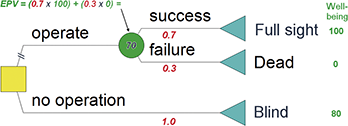
Obviously the operate option must be valued higher than zero and lower than 100. By taking a weighted average of those two numbers, we arrive at an expected preference value (EPV) of 70 (Figure 1.6).

Figure 1.6

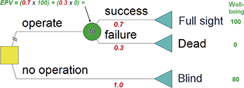
Figure 1.6 Long description

A node leads to two branches: operate and no operation. No operation has a p-value of 1.0, and leads to Blind (well-being is 80). Operate moves to a node labelled 70, with the formula E P V equals (0.7 times 100) plus (0.3 times 0). It branches into two paths: success (p-value of 0.7; leads to Fully sighted; well-being is 100) and failure (p-value of 0.3; leads to Dead; well-being is 0).

Now we’re ready to compare the options: ‘operate’ is at 70, ‘don’t operate’ is at 80, so choose not to operate. The cross-off mark indicates that the operate option is not the best choice. That’s only a 10-point difference in value, half the 20-point difference between blind and fully sighted, so maybe it’s worth thinking more deeply about that 80 for being blind. Best to talk to some blind people (as I have done in a project for the UK charity, Guide Dogs for the Blind, where I learned that many blind people don’t even feel particularly disadvantaged).

Now I want to ask you another question. What were you thinking of when you assigned the preference values of 100–80–0 to the consequences? Perhaps you were focused on your physical well-being and how well you could continue your present life. Fair enough. But if you were married, with children, perhaps you might also consider how well off your family would be as a separate consideration alongside your physical well-being. We’ll call it family well-being, defined as the extent of financial, social and psychological well-being for your family until your children have grown and left home. Now things get more complex, but see it through, back-tracking and reading again after seeing the final result, which comes later. It’s really all just simple arithmetic.

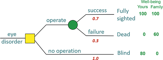
For this family criterion, what would your preferences be for the three consequences? If you remain fully sighted, you will continue as now, a score of 100, and being blind might well be the worst, a score of zero. If you die, your insurance could help your family to adapt after you die, perhaps sufficiently to sustain the family until the children are grown, but their social and psychological well-being will certainly be disrupted. You might take account of your spouse’s income, if you both work, the ages of your children, how your death might affect the children and the impact on grandparents, and any other considerations. For the purposes of illustration, let’s assume a score of 60. The new decision tree, expanded to take account of both criteria – your physical and family’s well-being – is shown in Figure 1.7.

Figure 1.7

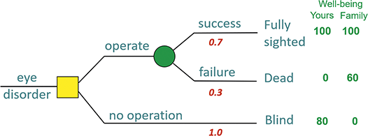
Figure 1.7 Long description

The context is an eye disorder, which leads to two branches: operate and no operation. No operation has a p-value of 1.0, and leads to Blind (well-being: Yours is 80, Family is 0). Operate branches into two paths: success (p-value of 0.7; leads to Fully sighted; well-being: Yours is 100, Family is 100) and failure (p-value of 0.3; leads to Dead; well-being: Yours is 0, Family is 60).

Considering only the scores under the family criterion, weight them by their probabilities:

$\text{EPV}\left(\text{Family}\right)=(100\times 0.7)+(60\times 0.3)=88$

Thus, operate is valued at 88, while ‘don’t operate’ is valued at 80. Now the operate option looks slightly more attractive. Obviously, the choice depends on which criterion you take into consideration. Can both be accommodated? Common sense and decision theory both say ‘yes’: by weighting the criteria, but they differ in how this is done.

Common sense might suggest more weight on your well-being and less on your family because your life is at stake. Indeed, if you consulted your family, they might tell you to ignore the financial consequences and express more aversion to risk than you feel. More generally, we take several criteria into account when choosing a place to live, buying a car, selecting a job or finding a school for our children.

Let’s see how in decision analysis it is done properly for the blind problem, as the method applies to all decisions in which multiple criteria, however dissimilar they seem to be, are a prominent feature of the choice problem.

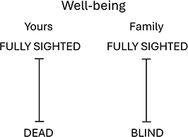
We’re going to weight the scales so we can add together the two weighted scores at the end of each branch of the decision tree. Then, we can repeat the above calculation, multiplying the new weighted values by the probabilities of the two events and adding the products. First, let’s look at the tops and bottoms of each scale, shown in Figure 1.8.

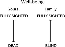
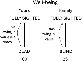
The best positions on both scales are Fully Sighted, but the worst position on the left scale is Dead, while it is Blind on the right scale. Which of those differences would you consider to be the biggest? That is, which swing in value is greater, from Dead to Fully Sighted for your own well-being, or from Blind to Fully Sighted for your family’s well-being? If that feels like comparing apples to oranges, it is actually the values of apples and oranges for the problem at hand that are being compared. Waldorf salads include apples, but not oranges, so oranges don’t add value for that kind of salad. As we will see for all decision models, it is the context of the decision that influences and establishes value.

So, now I ask, which scale represents the greatest swing in preference value from the worst to best position? To answer the question, consider now how big your difference in personal physical well-being is between being dead or fully sighted, compared to the well-being difference for your family between you being blind and fully sighted. In short, compare the worst-best difference on each scale and how much you care about those differences. That’s the key question for eliciting weights.

Many people to whom I’ve posed this problem don’t hesitate to say it’s the personal difference in well-being that matters most to them, a lot, so I give that a weight of 100. Compared to that, I ask, how big is the other increment of preference value? A typical answer is 25. In decision analysis, we call these numbers swing-weights (see Figure 1.9).

Figure 1.9

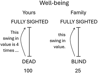
Figure 1.9 Long description

For the first, labelled Yours, the two ends are Dead and Fully sighted. An arrow from the bottom to the top indicates that this swing in value is 4 times that of the other one. The number 100 is written below. For the second, labelled Family, the two ends are Blind and Fully sighted. An arrow from the bottom to the top indicates that the swing in value of the other one is 4 times as much as this one. The number 25 is written below.

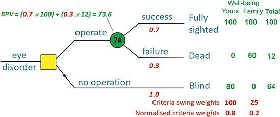
With those weights, when expressed as decimals that sum to 1.0, 0.8 and 0.2, a process called normalisation, we can now combine those 0–100 scales by weighting the preference values of the options, with the results shown in Figure 1.10 in the Total column. The weighted score at the end of each branch in the decision tree is then multiplied by the branch probability and summed, the EPV calculation, to give 73.6 (round up to 74; these aren’t precise figures). Compared to the 64 for Blind, this result now favours the operation.

Figure 1.10

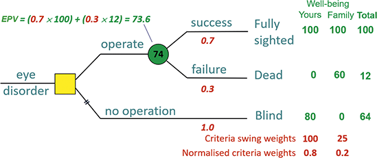
Figure 1.10 Long description

The context is an eye disorder, which leads to two branches: operate and no operation. No operation has a p-value of 1.0, and leads to Blind (well-being: Yours is 80, Family is 0, Total is 64). Operate leads to a node labelled 74, with the formula E P V equals (0.7 times 100) plus (0.3 times 12) equals 73.6. This node branches into two paths: success (p-value of 0.7; leads to Fully sighted; well-being: Yours is 100, Family is 100, Total is 100) and failure (p-value of 0.3; leads to Dead; well-being: Yours is 0, Family is 60, Total is 12). Criteria swing weights: Yours is 100, Family is 25. Normalised swing weights: Yours is 0.8, Family is 0.2.

The original preference value for operate has increased from 70 to 74, but the value for being blind has decreased from 80 to 64, leaving a value difference for this two-criteria model of only 10 units of preference value, and now operate is more preferred. Taking account of your family’s preferences changed the preferred option; multiple criteria and swing weights are indeed important ingredients. I’ll say more about swing-weighting in Chapter 5.

That completes the analysis of the blind problem. If it were your problem for real, I would now suggest you think about it for at least a couple weeks before making any decision and talk to those who might be affected by the consequences of your decision. Discuss it further with your family. Consider how you feel about the risk of an operation, how comfortable you are with the 70–30 chances, how much you would dread exposing yourself to the risk, and how others might feel about it.

The Ingredients of Good Decisions

Now let’s take stock of what we’ve learned as I summarise the ingredients used in modelling the blind problem. Some or all of 10 ingredients characterise every decision you take. That is the beauty of decision analysis, for it can be applied to any decision, whatever the topic. Even if you never construct a model of a decision, it will be helpful to keep in mind each of these ingredients, for they all play different roles, depending on the context and type of problem, in any final decision. The way we go about choosing the ingredients is often referred to as framing the problem.

The relative importance of the ingredients in framing is a matter of judgement and may change as a model develops. It’s wise to keep an open mind about which ingredients are appropriate for any given problem, because once you are committed to a particular combination of ingredients, it can be difficult to see you might be ignoring important issues, especially for experienced decision analysts who have learned which ingredients to use for certain problems. Bread requires yeast – unless it’s banana bread.

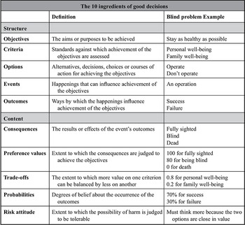
For now, let’s focus on the 10 ingredients of good decision making, five each for structure and content, all influenced by context (see Table 1.1).

Table 1.1The 10 ingredients of good decisions

Table 1.1 Long description

The table has 3 columns: Particulars, Definition, and Blind Problem Example. It reads as follows. Under Structure. Row 1. Objectives: The aims or purposes to be achieved; Stay as healthy as possible. Row 2. Criteria: Standards against which achievement of the objectives are assessed; Personal well-being, Family well-being. Row 3. Options: Alternatives, decisions, choices or courses of action for achieving the objectives; Operate, Don’t operate. Row 4. Events: Happenings that can influence achievement of the objectives; An operation. Row 5. Outcomes: Ways by which the happenings influence achievement of the objectives; Success, Failure. Under Content. Row 6. Consequences: The results or effects of the event’s outcomes; Fully sighted; Blind; Dead. Row 7. Preference values: Extent to which the consequences are judged to achieve the objectives; 100 for fully sighted, 80 for being blind, 0 for death. Row 8. Trade-offs: The extent to which more value on one criterion can be balanced by less on another; 0.8 for personal well-being, 0.2 for family well-being. Row 9. Probabilities: Degrees of belief about the occurrence of the outcomes; 70 percent for success, 30 percent for failure. Row 10. Risk attitude: Extent to which the possibility of harm is judged to be tolerable; Must think more because the two options are close in value.

This list of 10 ingredients is silent about the process of putting the ingredients together. Similar ingredients appear in many recipes, like flour, milk, eggs, sugar and salt for bread, pancakes and waffles. So different problems require different combinations of ingredients. Selecting the right ingredients and combining them properly is a matter of process, the subject of the chapters in Part III.

There are different ways of organising the structure and content of a decision model depending on the context of the problem, which is discussed in Chapter 12. Also, sometimes the options are given, while for other problems, the objectives and criteria are given. Uncertain events might need to be considered first, or a need to avoid disastrous consequences.

However, to begin helping your client, you start by exploring their sense of unease resulting from a growing concern about the discrepancy between the current situation and a desired future. Your role as a decision analyst is to help your client take decisions that will close or lessen the gap. The approach you take to develop the helping relationship is discussed in Part II.

The Grammar of Decision Making

At this point, I need to generalise the two calculations that gave a preference value of 74 to the operate option when both your physical well-being and your family’s well-being were being considered.

The point of this excursion is to show that decision modelling isn’t restricted to simple two-outcome uncertain events. I’ve found that when students are introduced to decision theory with the blind problem, or something similar, this can create the impression that all problems can be reduced to this simple form of choosing between an uncertain event versus a sure thing. Real problems are more complex, as we shall see in Part III.

When statisticians or decision analysts multiply values by probabilities, they call the sum of the products an ‘expected’ value, with the abbreviation ‘EV’. It doesn’t represent anybody’s psychological ‘expectation’, so I avoid the term when working with clients and will mostly not use it in this book, but when I do it means ‘weighted average’.

Statisticians also use the term ‘random variable’ as a generic term for a quantity whose numerical value is not yet known. Again, this term isn’t helpful in work with clients if you refer to preference values as random variables because there is nothing random about the numbers at the end of a decision tree, and clients don’t usually think of them as variable. Except for constants, any number in a decision analysis starts off as an uncertain quantity, a term that is self-explanatory, so I frequently use it.

If this were a problem with many options, events and criteria, it would be necessary to keep track of when to calculate what. The decision tree is a great way to visualise what to do and when, and I’m happy to report that computer programs are available to help you create the tree, populate it with the uncertain quantities we use, probabilities, weights and values, and then let the program do the calculating.² If you are a do-it-yourself sort of person and are familiar with spreadsheets, you could draw the tree on paper and then instruct the program to do the calculations. Many examples are given in Kirkwood’s excellent book.³

The Mathematics of Decision Analysis

Skip this section if you intend to rely on a decision tree program to do all the work for you. If you would like to see how to express the blind problem calculations in a single formula, read on. The following formulas constitute the grammar of decision analysis and can be generalised for any number of options, events and criteria. It’s done in four steps.

Step 1: Create the tree and convert it to a table with rows and columns that include the probabilities, values and swing weights. It would look something like Table 1.2 for the blind problem (check out the pattern of subscripts on the preference values; I’ll use these in the equations).

Table 1.2

Table 1.2 Long description

The table has 4 main columns with a few subcolumns: Step 1 (Options), Criteria (Consequences and j probabilities; Well being k equals 1; Family k equals 2), Step 2 (Weighted value sum), and Step 2 (Sums times probabilities). It reads as follows. Row 1: Operate i equals 1; Fully Sighted p1 equals 0.6; 100, v111; 100, v112; 100, v11; 73.6, v1. Row 2: Operate i equals 1; Dead p2 equals 0.4; 0, v121; 60, v122; 12, v12; blank. Row 3: Don’t operate i equals 2; Blind p3 equals 1.0; 80, v231; 0, v232; 64, v13; 64, v2. Swing weights: w1 equals 0.8; w2 equals 0.2.

Step 2: For each of the consequences, multiply the values associated with the criteria by the column swing weights and sum the products.

$V_{ij}={\displaystyle \sum }_k{w}_k{v}_{ijk}$

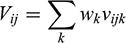
This step combines the preference values for each consequence into a single value. In the algebraic notation, it eliminates the k subscript.

Step 3: For each of the options’ consequences, multiply the weighted value sum calculated in Step 2 by the probability for each consequence and sum the products.

$E{V}_i={\displaystyle \sum }_j{p}_{ij}{V}_{ij}$

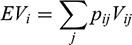
This step combines the single weighted preference value associated with each consequence into a single value for each option; it eliminates the j subscript. Because several values are multiplied by probabilities and summed, I’ve shown the result as an expected value as is common in statistics and decision theory.

Those two equations can be combined into one, which in application requires the doubly weighted sum to be carried out in the sequence of step 1 then 2:

$E{V}_i={\displaystyle \sum }_j{\displaystyle \sum }_k{p}_{ij}{v}_{ijk}$

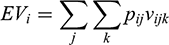
You might have noticed that the equations for the first two steps have one feature in common: they both weight a preference value with a number that extends from 0 to 1. If I were using a spreadsheet to do the computations, the computer wouldn’t know whether the number represented a probability or a swing weight. I take advantage of this feature in Chapter 5 for benefit-safety models of pain-killer drugs.

Step 4: Choose the option with the highest expected value. The equation for that is simple:

${\max }_{i}E{V}_i,\text{for i > 1}$

You ‘maximise’ the EV by choosing the bigger one. Note that to do that there must be two or more options. I have sometimes been asked to create a decision analysis model to justify a single option, which I explain can’t be done unless at least two options are being considered. A persuasive argument might do the job, but beware if someone introduces a new option that might be better.

A Framework for Creating Decision Models

You’ve now learned the fundamentals of decision analysis. The next step is to gain experience in applying that knowledge; learning the fundamentals of decision analysis is akin to learning a new language – it takes practice to become skilful. You’ve learned enough to apply it to simple situations, like the blind problem, perhaps with more options, more events and more criteria. The principles remain the same for larger problems.

Start with something small, just to practise. Something you could do entirely intuitively, which will most likely give you the answer you expected. Or perhaps not, in which case, go back and see why the model and your intuition disagree. A PhD graduate in decision theory whom I knew had received several job offers, and was about to decide on one, when I suggested to him that he try modelling it by using a software package developed by the staff of my Decision Analysis Unit. When he did, the best option was not the one he intuitively preferred. He then applied the software again, each day for a week, receiving the same result, and he finally realised this was caused by a fundamental conflict in his core personal values. He then thought more deeply about his life’s goals, resolved the value conflict, and chose an option he had originally dismissed.

Whatever you find from your initial attempts at modelling, keep at it and soon you will become fluent in this new language. I no longer have to look up familiar recipes in The Joy of Cooking, as I now know the ingredients, their amounts, and how to combine them to produce results. Even better, I now have the experience to know how to change the recipe to produce new and different results. That’s the main topic of Part III.

You may feel that the numbers for the blind problem were excessively precise, and I agree with you. I’ll say more about this in the next three chapters, but we are bound to accept imprecision in the numbers when making decisions about the future because the solid data we would like to have is not yet available; subjective judgement is required in assessing preference values, trade-off weights and probabilities. Those three quantities are not sitting in your client’s head, waiting to be plucked out. Rather, they are formed in the process of building and exploring the model, as Lichtenstein and Slovic pointed out in their important research compendium, The Construction of Preference.⁴ As we will see in Chapter 3, numerical quantities are the language of decision theory, and the intellectual effort of expressing preferences in numerical form helps one to form the preferences, making them explicit, finding inadequacies and inconsistencies, then changing or revising them.

A rough rule of thumb, derived mainly from experience, is that the precision of probabilities, scores or weights, expressed on a 0–100 scale, is about ±5. I applied that rule of thumb in considering the final results for the blind problem in comparing the 74 for operate and 64 for don’t operate. As an engineering student, I was taught to limit displays of results to significant figures that are within the limits of precision, so I mentally added 5 to 74 and subtracted 5 from 74, a range of 69 to 79. Then I did the same for the 64, giving 59 to 69. The low of 69 on the former is identical to the high on the latter, so I suggested more thinking about the problem for a couple of weeks before deciding (or revising the model).

Let’s now be explicit about the process for creating any decision model, which is shown here.

I’ll use these five process steps in the six recipes of Chapters 13 to 18, where the 10 ingredients of good decisions are applied in different ways and combinations for each type of problem. In the meantime, you might start honing your decision-making skills by applying what you’ve learned so far on a real problem of your own, or one of a friend or colleague.

It’s best if this is a real problem, otherwise it will be difficult or impossible to make the required assessments because the problem is hypothetical. You might help someone who is thinking of changing jobs, a young person looking for a job or a family needing a new kitchen appliance. It’s best to avoid the question of what car to buy, as cars are often expressions of the purchaser’s personality, which can cloud rational analysis!

The occasional client wants to know the origins of the concepts you use in modelling their decision problem, or you might be curious about the origins of the key ingredients for all decisions. If so, move on to Chapter 2 to discover the origins of decision analysis and learn why the three ingredients, preference values, trade-offs and probabilities, were not just arbitrarily chosen concepts.

Chapter 3 takes up the issue of how to establish that the numbers associated with the three ingredients can be said to meaningfully represent the property being measured. Or you could move to any of Chapters 4 to 6 for more information about the three ingredients and how to assess them. If you have a particular problem in mind, you might skip to Chapter 12, which describes the six types of decision models, to see if one of the other chapters in Part III could help you address your problem.

And since strategy is a continuing theme throughout the book, you could read Chapter 19 to learn more about strategic thinking.

Whichever chapter you go to next, I recommend that, at some point, you come back and read all six chapters of Part 1. A sound understanding of these chapters will provide a boost to your growing confidence in using this new language of decision analysis.

Summary

This chapter introduced the 10 ingredients to be considered if you are constructing a model that could help to resolve your client’s sense of unease, enabling him or her to take a decision. In modelling the blind problem, we’ve identified the 10 ingredients that are common to all decisions: five for the structure of the problem – objectives, criteria, options, events and outcomes; and five for the content – consequences, preference values, trade-offs, probabilities and risk attitude. All 10 require a degree of judgement for analysing a decision. The five structure ingredients establish what content must be considered, while the five content ingredients give magnitude and direction to the options.

The blind problem also introduced the ‘logical glue’ that enables preference values on the different criteria to be brought together. For problems dominated by multiple criteria, the logical glue is trade-off weights for the criteria that create a common unit of preference value, enabling them to be compared. If a problem is dominated by uncertainty, the logical glue is the probabilities of an option’s preference values that adjust the option’s preference values and combine them, enabling the options to be compared.

In applying the ingredients to a real problem, a framework can prevent errors of omission. The five-step framework for creating a decision model is a distillation of many frameworks reported in books and papers about decision analysis. In practice, a few more steps may be needed,⁵ depending on the type of problem, as you can see in Chapters 13 to 18.

At this point, you may well wonder how it is possible to reduce the complexity of taking decisions to just three numerical quantities. Where did they come from? Why these three and not others? What is the justification for the expected preference value model? These issues are addressed in the next chapter.