


1. Introduction
Fast radio bursts (FRBs) are short, highly energetic radio signals originating at cosmological distances. The relatively young field of FRBs has rapidly developed since their discovery in 2007 (Lorimer et al. Reference Lorimer, Bailes, McLaughlin, Narkevic and Crawford2007), now with thousands of sources detected (e.g. CHIME/FRB Collaboration et al. 2021) and of order a hundred localised to host galaxies (e.g. Rajwade et al. Reference Rajwade2022; Shannon et al. Reference Shannon2025; Sharma et al. Reference Sharma2024; CHIME/FRB Collaboration et al. 2025b; Pastor-Marazuela et al. Reference Pastor-Marazuela2025). Current research in this field is broadly focused in two directions: understanding the origins of these bursts, and using their observables to study the cosmology of our Universe. In this work, we focus on population studies of FRBs, which hold information regarding both facets, and place particular emphasis on probing the baryon content of the Milky Way halo (DM $_\mathrm{MW,halo}$
).
$_\mathrm{MW,halo}$
).
FRBs have found an incredible niche in cosmological science due to their unique ability to directly measure the baryon content of the Universe (e.g Thornton et al. Reference Thornton2013; Macquart et al. Reference Macquart2020; Glowacki & Lee Reference Glowacki and Lee2026). As electromagnetic radiation passes through ionised gas it experiences a frequency-dependent retardation. This is easily measured as an observable of the burst known as the dispersion measure (DM), which is directly proportional to the integrated electron column density along the line of sight. As baryons trace the electron distribution of the Universe, this allows FRBs to map out the complete cosmological baryon distribution, which is otherwise unobservable (Macquart et al. Reference Macquart2020; Khrykin et al. Reference Khrykin2024; Connor et al. Reference Connor2025).
Most FRB studies focus on understanding the contribution of intergalactic and circumgalactic media (IGM and CGM) to the cosmological DM budget. However, FRBs are also one of the few direct probes of the Milky Way halo (Prochaska & Zheng Reference Prochaska and Zheng2019; Keating & Pen Reference Keating and Pen2020; Platts, Prochaska, & Law Reference Platts, Prochaska and Law2020; Cook et al. Reference Cook2023; Ravi et al. Reference Ravi2025). Measuring the baryonic content and distribution of the Galactic halo is notoriously difficult due to the diffuse nature of the plasma contained within it, existing in a range of phases with temperatures $T \sim 10^4$
–
$T \sim 10^4$
– $10^7$
K. Typically, cool gas (
$10^7$
K. Typically, cool gas ( $T\lt10^4$
K) is clumpy and observable through 21 cm HI emission, warm and warm-hot (
$T\lt10^4$
K) is clumpy and observable through 21 cm HI emission, warm and warm-hot ( $10^4 \lt T \lt 10^6$
K) gas is observable through H
$10^4 \lt T \lt 10^6$
K) gas is observable through H $\alpha$
emission lines and absorption lines from quasi-stellar background objects, and hot (
$\alpha$
emission lines and absorption lines from quasi-stellar background objects, and hot ( $T\gt10^6$
K) gas is observable through X-ray emission and absorption lines of highly ionised metals, e.g. O
$T\gt10^6$
K) gas is observable through X-ray emission and absorption lines of highly ionised metals, e.g. O $^{+7}$
.
$^{+7}$
.
Current literature suggests that gas in lower temperature phases ( $T\lt10^6$
K) does not contribute significantly (
$T\lt10^6$
K) does not contribute significantly ( $\lt15\%$
) to the total Galactic baryon budget (e.g. Das et al. Reference Das, Mathur, Gupta, Nicastro and Krongold2021) and hence X-ray emission and absorption analyses are currently the best estimators for the total electron content. X-ray emission spectroscopy is a direct observation of the gas in the Milky Way and so samples large areas of the sky without the need for a background source (e.g. Nakashima et al. Reference Nakashima2018). However, it is biased towards denser gas and higher emissivity, meaning it only probes a subset of the total gas in the halo.
$\lt15\%$
) to the total Galactic baryon budget (e.g. Das et al. Reference Das, Mathur, Gupta, Nicastro and Krongold2021) and hence X-ray emission and absorption analyses are currently the best estimators for the total electron content. X-ray emission spectroscopy is a direct observation of the gas in the Milky Way and so samples large areas of the sky without the need for a background source (e.g. Nakashima et al. Reference Nakashima2018). However, it is biased towards denser gas and higher emissivity, meaning it only probes a subset of the total gas in the halo.
Conversely, X-ray absorption using background quasars does not have a density or emissivity bias. However, this only samples a small area in the sky due to the necessity for an X-ray bright quasar as a back-light (e.g. Fang et al. Reference Fang, Buote, Bullock and Ma2015). Furthermore, these rely on metal lines, which implies an inherent degeneracy between the assumed or estimated metallicity and the total mass.
DM is a powerful observable because it is a direct measurement of all ionised gas along the line of sight, regardless of the quantity, phase and metallicity of the gas. For a predominantly ionised gas, as anticipated for the halo of our Galaxy, DM provides an estimate of the baryonic mass along a given sightline. Additionally, as the number of FRB sightlines across the sky continues to rapidly rise, one may probe directional dependences. However, a significant limitation is the inability to disentangle the distribution of electrons along a given sightline, although such a degeneracy could be broken by other measures such as scattering in the future (Cordes, Ocker, & Chatterjee Reference Cordes, Ocker and Chatterjee2022; Mas-Ribas & James Reference Mas-Ribas and James2025. The measured DM of an FRB has contributions from plasma in the local environment of the progenitor, the interstellar medium (ISM) and the halo of the host galaxy (DM $_\mathrm{host}$
), cosmological gas in the IGM and the CGM of intervening halos (DM
$_\mathrm{host}$
), cosmological gas in the IGM and the CGM of intervening halos (DM $_\mathrm{cosmic}$
), the Milky Way halo (DM
$_\mathrm{cosmic}$
), the Milky Way halo (DM $_\mathrm{MW,halo}$
) and the Milky Way ISM (DM
$_\mathrm{MW,halo}$
) and the Milky Way ISM (DM $_\mathrm{MW,ISM}$
). DM is a measure of the integrated column density of electrons and, as such, cannot determine the relative contributions from each component. Therefore, meaningful constraints on the Galactic halo dispersion measure DM
$_\mathrm{MW,ISM}$
). DM is a measure of the integrated column density of electrons and, as such, cannot determine the relative contributions from each component. Therefore, meaningful constraints on the Galactic halo dispersion measure DM $_\mathrm{MW,halo}$
require specially designed experiments.
$_\mathrm{MW,halo}$
require specially designed experiments.
One of these is to analyse the distribution of observed FRB DMs and estimate the minimum value after accounting for the Galactic ISM contribution. This minimum DM provides an upper limit to DM $_\mathrm{MW,halo}$
subject to the unknown host and IGM contributions. Platts et al. (Reference Platts, Prochaska and Law2020) and Cook et al. (Reference Cook2023) used this technique to infer DM
$_\mathrm{MW,halo}$
subject to the unknown host and IGM contributions. Platts et al. (Reference Platts, Prochaska and Law2020) and Cook et al. (Reference Cook2023) used this technique to infer DM $_\mathrm{MW,halo}$ $\lt 123$
pc cm
$\lt 123$
pc cm $^{-3}$
and
$^{-3}$
and $\lt 52$
–111 pc cm
$\lt 52$
–111 pc cm $^{-3}$
, respectively. A variant of this approach is to restrict to FRBs associated at high confidence to a host galaxy with a measured redshift. In this case, one may estimate the cosmic dispersion measure DM
$^{-3}$
, respectively. A variant of this approach is to restrict to FRBs associated at high confidence to a host galaxy with a measured redshift. In this case, one may estimate the cosmic dispersion measure DM $_\mathrm{cosmic}$
and can even limit its contribution by restricting to very nearby (low redshift) FRBs. Ravi et al. (Reference Ravi2025) took this approach with FRB 20220319D to infer DM
$_\mathrm{cosmic}$
and can even limit its contribution by restricting to very nearby (low redshift) FRBs. Ravi et al. (Reference Ravi2025) took this approach with FRB 20220319D to infer DM $_\mathrm{MW,halo}$ $\lt 47.3$
pc cm
$\lt 47.3$
pc cm $^{-3}$
.
$^{-3}$
.
These techniques are currently limited to a few sightlines and are therefore subject to uncertainties in DM $_\mathrm{MW,ISM}$
along the individual sightlines, which directly translates to uncertainty in DM
$_\mathrm{MW,ISM}$
along the individual sightlines, which directly translates to uncertainty in DM $_\mathrm{MW,halo}$
. Furthermore, DM
$_\mathrm{MW,halo}$
. Furthermore, DM $_\mathrm{MW,halo}$
may be anisotropic (Nakashima et al. Reference Nakashima2018; Kaaret et al. Reference Kaaret2020; Yamasaki & Totani Reference Yamasaki and Totani2020; Das et al. Reference Das, Mathur, Gupta, Nicastro and Krongold2021; Huang et al. Reference Huang, Lee, Libeskind, Simha, Valade and Prochaska2025), and these works (Platts et al. Reference Platts, Prochaska and Law2020; Cook et al. Reference Cook2023; Ravi et al. Reference Ravi2025), which sample single or a few sightlines, are subjected to such halo fluctuations. As such, analyses of the lowest DM FRBs can inform us about the minimum densities within the Milky Way halo, but may or may not be indicative of a characteristic contribution. As the Canadian Hydrogen Intensity Mapping Experiment (CHIME) now have operational outriggers (Chime/Frb Collaboration et al. 2025a) to localise their detections, we expect the number of localised, nearby FRBs to increase substantially and as we fill out this parameter space, such a sample will make these methods significantly more robust in the future.
$_\mathrm{MW,halo}$
may be anisotropic (Nakashima et al. Reference Nakashima2018; Kaaret et al. Reference Kaaret2020; Yamasaki & Totani Reference Yamasaki and Totani2020; Das et al. Reference Das, Mathur, Gupta, Nicastro and Krongold2021; Huang et al. Reference Huang, Lee, Libeskind, Simha, Valade and Prochaska2025), and these works (Platts et al. Reference Platts, Prochaska and Law2020; Cook et al. Reference Cook2023; Ravi et al. Reference Ravi2025), which sample single or a few sightlines, are subjected to such halo fluctuations. As such, analyses of the lowest DM FRBs can inform us about the minimum densities within the Milky Way halo, but may or may not be indicative of a characteristic contribution. As the Canadian Hydrogen Intensity Mapping Experiment (CHIME) now have operational outriggers (Chime/Frb Collaboration et al. 2025a) to localise their detections, we expect the number of localised, nearby FRBs to increase substantially and as we fill out this parameter space, such a sample will make these methods significantly more robust in the future.
Yet another method, and the one considered here, is to constrain gas profiles using a large number of FRBs with precise redshifts (McQuinn Reference McQuinn2014). Such population studies require a large number of FRBs to obtain such estimates. In this work, we place constraints on DM $_\mathrm{MW,halo}$
using a large sample of 98 FRBs and 32 associated redshifts while simultaneously fitting other unknown population parameters. Our approach is statistical in nature and, in principle, allows for modelling the halo with an inhomogeneous density distribution.
$_\mathrm{MW,halo}$
using a large sample of 98 FRBs and 32 associated redshifts while simultaneously fitting other unknown population parameters. Our approach is statistical in nature and, in principle, allows for modelling the halo with an inhomogeneous density distribution.
In Section 2, we give an overview of the data that we use and our choices of data cuts. We also justify model choices and outline changes to the analysis techniques presented in James et al. (Reference James2022a) and Hoffmann et al. (Reference Hoffmann2025). We present our results in Section 3 and conclude in Section 5.
2. Methods and data
This work is a continuation of previous publications using the zDM code base (James et al. Reference James2022a). The specific implementations are identical to those described in James et al. (Reference James2022b) and Hoffmann et al. (Reference Hoffmann2025) except where otherwise specified. We model DM $_\mathrm{host}$
as a log-normal distribution with mean
$_\mathrm{host}$
as a log-normal distribution with mean $\mu_\mathrm{host}$
and standard deviation
$\mu_\mathrm{host}$
and standard deviation $\sigma_\mathrm{host}$
as free parameters; the cosmic evolution of FRB progenitors is modeled by the cosmic star formation rate to some power n; the spectral dependence is denoted by
$\sigma_\mathrm{host}$
as free parameters; the cosmic evolution of FRB progenitors is modeled by the cosmic star formation rate to some power n; the spectral dependence is denoted by $\alpha$
where we use a ‘rate-interpretation’ (James et al. Reference James2022a) which is further discussed in Section 2.2; we model the luminosity function as an upper-incomplete Gamma function with slope
$\alpha$
where we use a ‘rate-interpretation’ (James et al. Reference James2022a) which is further discussed in Section 2.2; we model the luminosity function as an upper-incomplete Gamma function with slope $\gamma$
, exponential cutoff beginning at
$\gamma$
, exponential cutoff beginning at $E_{\mathrm{max}}$
and a hard-cutoff at some minimum energy
$E_{\mathrm{max}}$
and a hard-cutoff at some minimum energy $E_{\mathrm{min}}$
. We additionally assume a flat
$E_{\mathrm{min}}$
. We additionally assume a flat $\Lambda$
CDM model for our Universe and utilise measurements from Planck. We model telescope and algorithm biases (e.g. Hoffmann et al. Reference Hoffmann2024) for each telescope, and construct a DM model as in Equation (1). Using this model, we conduct a full likelihood analysis in a Markov-Chain Monte-Carlo (MCMC) framework to simultaneously constrain each of the unknown parameters.
$\Lambda$
CDM model for our Universe and utilise measurements from Planck. We model telescope and algorithm biases (e.g. Hoffmann et al. Reference Hoffmann2024) for each telescope, and construct a DM model as in Equation (1). Using this model, we conduct a full likelihood analysis in a Markov-Chain Monte-Carlo (MCMC) framework to simultaneously constrain each of the unknown parameters.
2.1. Data
We use the same base data as Hoffmann et al. (Reference Hoffmann2025) with the addition of the data described in Table 2. This data includes FRBs from blind searches using the Australian SKA Pathfinder (ASKAP) telescope as part of the Commensal Real-time ASKAP Fast Transients (CRAFT) survey in the Fly’s Eye and incoherent sum (ICS) modes, the Parkes Murriyang telescope, the Five-hundred meter Apperture Spherical radio Telescope (FAST) and the Deep Synoptic Array (DSA). The CRAFT/ICS survey is modelled in 3 different observing bands.
We apply the same data selection cuts as per Hoffmann et al. (Reference Hoffmann2025), where we exclude redshift information for FRBs with extragalactic DM (DM $_\mathrm{EG}$ $=\mathrm{DM_{total}} -$
DM
$=\mathrm{DM_{total}} -$
DM $_\mathrm{MW,ISM}$ $-\langle$
DM
$-\langle$
DM $_\mathrm{MW,halo}$ $\rangle$
) exceeding that of the lowest, hostless FRB in the given survey. This cut is applied to the DSA dataset as it is unclear why each FRB does not have an associated redshift, and hence we cannot include them without bias. We do not need to apply the same cut to FRBs detected with ASKAP, as the reason they do not have an associated redshift is due to the host galaxies not being followed up yet, and hence, there is no bias against high-redshift, low-DM objects. For the same reason, we now also include the redshift FRB 20171020A, which we previously excluded.
$\rangle$
) exceeding that of the lowest, hostless FRB in the given survey. This cut is applied to the DSA dataset as it is unclear why each FRB does not have an associated redshift, and hence we cannot include them without bias. We do not need to apply the same cut to FRBs detected with ASKAP, as the reason they do not have an associated redshift is due to the host galaxies not being followed up yet, and hence, there is no bias against high-redshift, low-DM objects. For the same reason, we now also include the redshift FRB 20171020A, which we previously excluded.
We apply an additional Galactic latitude cut of $|b| \gt 20^\circ$
as low-latitude FRBs have unreliable estimates for DM
$|b| \gt 20^\circ$
as low-latitude FRBs have unreliable estimates for DM
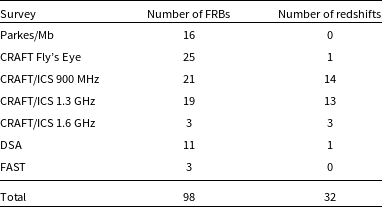
 $_\mathrm{MW,ISM}$
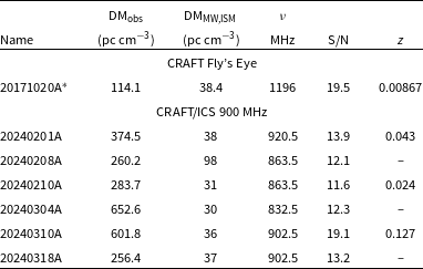
which can bias our results (see Section 2.4 for a further explanation). Given these cuts, we utilise a total of 98 FRBs and associated spectroscopic redshifts for 32 of them. A breakdown of the number of FRBs used in each survey is given in Table 1. This data includes 6 more FRBs detected in 2024 during the CRAFT/ICS 900 MHz survey (Shannon et al. Reference Shannon2025) and the redshift of FRB 20171020A detected during the CRAFT Fly’s Eye survey, which was previously excluded (Lee-Waddell et al. Reference Lee-Waddell2023). The details for these FRBs are presented in Table 2.
$_\mathrm{MW,ISM}$
which can bias our results (see Section 2.4 for a further explanation). Given these cuts, we utilise a total of 98 FRBs and associated spectroscopic redshifts for 32 of them. A breakdown of the number of FRBs used in each survey is given in Table 1. This data includes 6 more FRBs detected in 2024 during the CRAFT/ICS 900 MHz survey (Shannon et al. Reference Shannon2025) and the redshift of FRB 20171020A detected during the CRAFT Fly’s Eye survey, which was previously excluded (Lee-Waddell et al. Reference Lee-Waddell2023). The details for these FRBs are presented in Table 2.
The total number of FRBs and the corresponding number of redshifts that we use in our analysis from each survey after the given cuts.

Information used in addition to those in Hoffmann et al. (Reference Hoffmann2025). FRBs that are below the Galactic latitude cut of $|b| \lt 20^\circ$
are not included. FRB 20171020A was used in previous analyses, however, the redshift was not previously utilised. The redshift was taken from Lee-Waddell et al. (Reference Lee-Waddell2023). The FRBs listed from the CRAFT/ICS 900 MHz survey were not used at all in previous analyses and are further described in Shannon et al. (Reference Shannon2025).
$|b| \lt 20^\circ$
are not included. FRB 20171020A was used in previous analyses, however, the redshift was not previously utilised. The redshift was taken from Lee-Waddell et al. (Reference Lee-Waddell2023). The FRBs listed from the CRAFT/ICS 900 MHz survey were not used at all in previous analyses and are further described in Shannon et al. (Reference Shannon2025).

Although more FRBs and localisations from DSA and MeerKAT have been released, a complete sample has not been made available, which can introduce bias in our results. In particular, it is easier to detect host galaxies that are at a lower redshift, and so we would preferentially obtain low-redshift host galaxies for a given DM. Hence, until a full sample of all detected FRBs is made available, these data sets cannot be included in our analysis without bias. Additionally, providing the reasons as to why FRBs have not been associated with a host galaxy can allow more redshifts to be used, as the bias is only present if the redshift is absent due to a particularly distant or faint host galaxy. Thus, we strongly encourage authors to publish such information in future publications, and we are committed to providing it.
CHIME has the largest number of detected FRBs to date (CHIME/FRB Collaboration et al. 2021), with an increasing number being accurately localised to host galaxies (CHIME/FRB Collaboration et al. 2024; CHIME/FRB Collaboration et al. 2025b). Due to its large field of view but relatively lower sensitivity, many of these FRBs are in the local Universe, including FRB 20200120E (Bhardwaj et al. Reference Bhardwaj2021) located in M81 and FRB 20250316A (CHIME/FRB Collaboration et al. 2025b) at a distance of 40 Mpc. In principle, these FRBs are the most constraining on DM $_\mathrm{MW,halo}$
and hence would increase our constraining power significantly. However, CHIME has a unique bias towards detecting repeaters, which must be explicitly modelled (James Reference James2023). As this model is currently not fully functional within zDM, we cannot include CHIME FRBs without bias, and so leave this analysis to future work (Hoffmann et al. in preparation).
$_\mathrm{MW,halo}$
and hence would increase our constraining power significantly. However, CHIME has a unique bias towards detecting repeaters, which must be explicitly modelled (James Reference James2023). As this model is currently not fully functional within zDM, we cannot include CHIME FRBs without bias, and so leave this analysis to future work (Hoffmann et al. in preparation).
2.2. Parameters
We adopt the same base parameters and priors for FRB population modelling as Hoffmann et al. (Reference Hoffmann2025), except for our prior on the spectral index $\alpha$
. We have changed this prior because we exclude information about the number of events detected in a given survey, P(N). While P(N) does contain useful information, the difficulty in characterising the observational time spent on the sky has posed many challenges, and we consider it an unreliable quantity. Even amongst surveys conducted with ASKAP, the rates that have been obtained have been inconsistent (Shannon et al. Reference Shannon2025; Hoffmann et al. Reference Hoffmann2025). Without P(N), we cannot obtain good constraints on
$\alpha$
. We have changed this prior because we exclude information about the number of events detected in a given survey, P(N). While P(N) does contain useful information, the difficulty in characterising the observational time spent on the sky has posed many challenges, and we consider it an unreliable quantity. Even amongst surveys conducted with ASKAP, the rates that have been obtained have been inconsistent (Shannon et al. Reference Shannon2025; Hoffmann et al. Reference Hoffmann2025). Without P(N), we cannot obtain good constraints on $\alpha$
, and so we place a restrictive prior on it. Results previously obtained from population studies have had large (
$\alpha$
, and so we place a restrictive prior on it. Results previously obtained from population studies have had large ( $\sim$
100%) uncertainties (e.g. James et al. Reference James2022a; Shin et al. Reference Shin2023; Hoffmann et al. Reference Hoffmann2025), and thus, values of
$\sim$
100%) uncertainties (e.g. James et al. Reference James2022a; Shin et al. Reference Shin2023; Hoffmann et al. Reference Hoffmann2025), and thus, values of $\alpha$
obtained through direct analysis of FRB spectra are expected to be more reliable. Hence, we defer to priors from such studies.
$\alpha$
obtained through direct analysis of FRB spectra are expected to be more reliable. Hence, we defer to priors from such studies.
When considering other studies, it is important to understand the interpretation for $\alpha$
that they imply. Our model broadly modifies the detection rate of FRBs at a given frequency (
$\alpha$
that they imply. Our model broadly modifies the detection rate of FRBs at a given frequency ( $\nu$
) by
$\nu$
) by $\nu^{\alpha}$
. As discussed in James et al. (Reference James2022a), for a negative
$\nu^{\alpha}$
. As discussed in James et al. (Reference James2022a), for a negative $\alpha$
, this can be interpreted as:
$\alpha$
, this can be interpreted as:
-
1. Assuming all bursts are broadband, then lower frequencies contain more energy (spectral index interpretation; $\alpha_{\mathrm{SI}}$
).
$\alpha_{\mathrm{SI}}$
). -
2. Assuming bursts are narrowband, then there is a greater number of bursts at lower frequencies but with similar energies (rate interpretation;
$\alpha_{\mathrm{R}}$
).


Previously, we have used a rate interpretation due to its lower computational requirements, however, most measurements in the literature use a spectral index interpretation. We also note that the choice of model primarily affects n and $\alpha$
itself, while not having large impacts on the other parameters, including those coming from the DM budget (Hoffmann et al. Reference Hoffmann2025).
$\alpha$
itself, while not having large impacts on the other parameters, including those coming from the DM budget (Hoffmann et al. Reference Hoffmann2025).
The first measurement of $\alpha$
was taken by Macquart et al. (Reference Macquart2019) who examined spectra from 23 FRBs detected by ASKAP as part of the Commensal Real-time ASKAP Fast Transients (CRAFT) survey and found
$\alpha$
was taken by Macquart et al. (Reference Macquart2019) who examined spectra from 23 FRBs detected by ASKAP as part of the Commensal Real-time ASKAP Fast Transients (CRAFT) survey and found $\alpha_{\mathrm{SI}} = -1.5^{+0.2}_{-0.3}$
, corresponding to
$\alpha_{\mathrm{SI}} = -1.5^{+0.2}_{-0.3}$
, corresponding to $\alpha_{\mathrm{R}} = -0.63 \pm 0.3$
(James et al. Reference James2022a). More recently, Shannon et al. (Reference Shannon2025) examined the frequency dependence of the FRB event rate and noted that we have poor constraints of
$\alpha_{\mathrm{R}} = -0.63 \pm 0.3$
(James et al. Reference James2022a). More recently, Shannon et al. (Reference Shannon2025) examined the frequency dependence of the FRB event rate and noted that we have poor constraints of $\alpha_{\mathrm{SI}} = -0.3^{+1.4}_{-1.6}$
for the extended CRAFT incoherent sum (ICS) observations. Similar studies using 62 broadband FRBs detected by the CHIME found
$\alpha_{\mathrm{SI}} = -0.3^{+1.4}_{-1.6}$
for the extended CRAFT incoherent sum (ICS) observations. Similar studies using 62 broadband FRBs detected by the CHIME found $\alpha_{\mathrm{SI}} = -0.98 \pm 0.05$
(Pleunis et al. in prep), but Cui et al. (Reference Cui, James, Li and Zhang2025) measure a steeper value of
$\alpha_{\mathrm{SI}} = -0.98 \pm 0.05$
(Pleunis et al. in prep), but Cui et al. (Reference Cui, James, Li and Zhang2025) measure a steeper value of $\alpha = -2.29 \pm 0.29$
with the CHIME sample when not restricting their analysis to broadband pulses (and hence being closer to
$\alpha = -2.29 \pm 0.29$
with the CHIME sample when not restricting their analysis to broadband pulses (and hence being closer to $\alpha_{\mathrm{R}}$
). As such, while using the rate interpretation, we apply a uniform prior on
$\alpha_{\mathrm{R}}$
). As such, while using the rate interpretation, we apply a uniform prior on $\alpha_{\mathrm{R}}$
of
$\alpha_{\mathrm{R}}$
of $-0.5$
to
$-0.5$
to $-2.5$
and do not utilise P(N) any longer.
$-2.5$
and do not utilise P(N) any longer.
All other priors are unrestrictive except for the Hubble constant, $H_0$
, on which we impose a uniform prior of 66.9 to 73.08 km
$H_0$
, on which we impose a uniform prior of 66.9 to 73.08 km $\mathrm{s}^{-1}$ $\mathrm{Mpc}^{-1}$
: a window spanning 1
$\mathrm{Mpc}^{-1}$
: a window spanning 1 $\sigma$
either side of the best estimates from Riess et al. (Reference Riess2022) and the Planck Collaboration et al. (2020).
$\sigma$
either side of the best estimates from Riess et al. (Reference Riess2022) and the Planck Collaboration et al. (2020).
Additionally, in this work, we are primarily interested in finding constraints on DM $_\mathrm{MW,halo}$
. As such, we allow the mean value of DM
$_\mathrm{MW,halo}$
. As such, we allow the mean value of DM $_\mathrm{MW,halo}$
to vary as a free parameter while imposing a uniform linear prior from 0 to 100 pc cm
$_\mathrm{MW,halo}$
to vary as a free parameter while imposing a uniform linear prior from 0 to 100 pc cm $^{-3}$
. We find that there is no significant difference when using log or linear priors on DM
$^{-3}$
. We find that there is no significant difference when using log or linear priors on DM $_\mathrm{MW,halo}$
, and as the summation is fundamentally linear (see Equation 1), we choose to use a linear uniform prior. Alternatively,
$_\mathrm{MW,halo}$
, and as the summation is fundamentally linear (see Equation 1), we choose to use a linear uniform prior. Alternatively, $\mu_\mathrm{host}$
and
$\mu_\mathrm{host}$
and $\sigma_\mathrm{host}$
use log-uniform priors to describe the log-normal distribution of DM
$\sigma_\mathrm{host}$
use log-uniform priors to describe the log-normal distribution of DM $_\mathrm{host}$
.
$_\mathrm{host}$
.
2.3. Degeneracy of DM
$_\mathrm{MW,halo}$
and DM
$_\mathrm{host}$


We model the total DM of each FRB as
 \begin{equation} \mathrm{DM_{total} = DM_{MW,ISM} + DM_{MW,halo} + DM_{cosmic}} + \frac{\mathrm{DM_{host}}}{1+z}, \end{equation}
with contributions from the Milky Way (ISM), the Milky Way halo, cosmic ionised gas and the host galaxy, respectively. Of these, DM $_\mathrm{MW,halo}$
and DM
$_\mathrm{MW,halo}$
and DM $_\mathrm{host}$
are poorly constrained, and hence we fit for them in our analysis. We model the distribution of DM
$_\mathrm{host}$
are poorly constrained, and hence we fit for them in our analysis. We model the distribution of DM $_\mathrm{MW,halo}$
values as a linear-normal distribution with a variable mean and a fixed standard deviation of 15 pc cm
$_\mathrm{MW,halo}$
values as a linear-normal distribution with a variable mean and a fixed standard deviation of 15 pc cm $^{-3}$
as discussed in Section 2.4, and DM
$^{-3}$
as discussed in Section 2.4, and DM $_\mathrm{host}$
as a log-normal distribution with mean (
$_\mathrm{host}$
as a log-normal distribution with mean ( $\mu_\mathrm{host}$
) and standard deviation (
$\mu_\mathrm{host}$
) and standard deviation ( $\sigma_\mathrm{host}$
) as free parameters. We choose a log-normal distribution for the host galaxy, as FRBs can be found far outside their galaxies’ ISMs (e.g. Kirsten et al. Reference Kirsten2022), and hence DM
$\sigma_\mathrm{host}$
) as free parameters. We choose a log-normal distribution for the host galaxy, as FRBs can be found far outside their galaxies’ ISMs (e.g. Kirsten et al. Reference Kirsten2022), and hence DM $_\mathrm{host}$
has a hard cutoff at 0 pc cm
$_\mathrm{host}$
has a hard cutoff at 0 pc cm $^{-3}$
but no effective upper limit allowing an upwards tail. On the contrary, the Earth is embedded well within the Galactic halo, and so we expect relatively consistent values of DM
$^{-3}$
but no effective upper limit allowing an upwards tail. On the contrary, the Earth is embedded well within the Galactic halo, and so we expect relatively consistent values of DM $_\mathrm{MW,halo}$
. Ultimately, when experimenting with linear-normal and log-normal distributions of DM
$_\mathrm{MW,halo}$
. Ultimately, when experimenting with linear-normal and log-normal distributions of DM $_\mathrm{MW,halo}$
, our results did not differ significantly and so this choice is not significant.
$_\mathrm{MW,halo}$
, our results did not differ significantly and so this choice is not significant.
Results from the MCMC analysis including FAST, DSA and CRAFT FRBs. The parameters are identical to those described in Table 3.

Although DM $_\mathrm{MW,halo}$
and DM
$_\mathrm{MW,halo}$
and DM $_\mathrm{host}$
have similar effects, the difference in the chosen functional form of their distributions and the
$_\mathrm{host}$
have similar effects, the difference in the chosen functional form of their distributions and the $(1+z)^{-1}$
weighting on DM
$(1+z)^{-1}$
weighting on DM $_\mathrm{host}$
allows this degeneracy to be broken, given a sufficient number of FRBs. Of course, if the Universe conspires FRB host galaxies to have DM
$_\mathrm{host}$
allows this degeneracy to be broken, given a sufficient number of FRBs. Of course, if the Universe conspires FRB host galaxies to have DM $_\mathrm{host}$
with a redshift dependence that approaches DM
$_\mathrm{host}$
with a redshift dependence that approaches DM $_\mathrm{host}$ $\sim (1+z)$
, then the degeneracy between these two components will be more difficult to resolve.
$\sim (1+z)$
, then the degeneracy between these two components will be more difficult to resolve.
2.4. DM
$_\mathrm{MW}$
uncertainties

We previously demonstrated that large uncertainties in DM $_\mathrm{MW,ISM}$
introduce significant uncertainties in cosmological parameters such as
$_\mathrm{MW,ISM}$
introduce significant uncertainties in cosmological parameters such as $H_0$
(Hoffmann et al. Reference Hoffmann2025). As such, it is important to minimise these errors. In particular, sightlines passing through the Galactic plane have significantly more variation than those at high Galactic latitudes. While we do implement a percentage uncertainty on DM
$H_0$
(Hoffmann et al. Reference Hoffmann2025). As such, it is important to minimise these errors. In particular, sightlines passing through the Galactic plane have significantly more variation than those at high Galactic latitudes. While we do implement a percentage uncertainty on DM $_\mathrm{MW,ISM}$
to account for this, this causes underfluctuations to be considered more precise and overfluctuations less precise, resulting in a bias towards lower DM
$_\mathrm{MW,ISM}$
to account for this, this causes underfluctuations to be considered more precise and overfluctuations less precise, resulting in a bias towards lower DM $_\mathrm{MW,ISM}$
values. Additionally, the fluctuations at low galactic latitude are significantly greater (even when considering percentage uncertainties) than those at high latitude, and hence applying a uniform uncertainty is not sensible. Thus, in this analysis, we exclude all FRBs detected below a galactic latitude of
$_\mathrm{MW,ISM}$
values. Additionally, the fluctuations at low galactic latitude are significantly greater (even when considering percentage uncertainties) than those at high latitude, and hence applying a uniform uncertainty is not sensible. Thus, in this analysis, we exclude all FRBs detected below a galactic latitude of $|b| \lt 20^\circ$
. Above this latitude, uncertainties in Galactic DM contributions are minimised due to smoother gas distributions and the rarity of discrete structures (Ocker, Cordes, & Chatterjee Reference Ocker, Cordes and Chatterjee2020; Ocker et al. Reference Ocker, Anderson, Lazio, Cordes and Ravi2024). As such, we reduce the 50% uncertainty on DM
$|b| \lt 20^\circ$
. Above this latitude, uncertainties in Galactic DM contributions are minimised due to smoother gas distributions and the rarity of discrete structures (Ocker, Cordes, & Chatterjee Reference Ocker, Cordes and Chatterjee2020; Ocker et al. Reference Ocker, Anderson, Lazio, Cordes and Ravi2024). As such, we reduce the 50% uncertainty on DM $_\mathrm{MW,ISM}$
estimated from Schnitzeler (Reference Schnitzeler2012) to 20%, but otherwise implement this uncertainty using the same method as Hoffmann et al. (Reference Hoffmann2025).
$_\mathrm{MW,ISM}$
estimated from Schnitzeler (Reference Schnitzeler2012) to 20%, but otherwise implement this uncertainty using the same method as Hoffmann et al. (Reference Hoffmann2025).
We also note that little is known about DM $_\mathrm{MW,halo}$
, particularly regarding its distribution and homogeneity. While we do fit for the average value of DM
$_\mathrm{MW,halo}$
, particularly regarding its distribution and homogeneity. While we do fit for the average value of DM $_\mathrm{MW,halo}$
, we do not account for fluctuations along different lines of sight (nor asymmetry with Galactic latitude or any other geometric parameter; see below). However, X-ray measurements have observed such variations, with Das et al. (Reference Das, Mathur, Gupta, Nicastro and Krongold2021) combining X-ray absorption and emission measurements obtaining a mean DM
$_\mathrm{MW,halo}$
, we do not account for fluctuations along different lines of sight (nor asymmetry with Galactic latitude or any other geometric parameter; see below). However, X-ray measurements have observed such variations, with Das et al. (Reference Das, Mathur, Gupta, Nicastro and Krongold2021) combining X-ray absorption and emission measurements obtaining a mean DM $_\mathrm{MW,halo}$
of
$_\mathrm{MW,halo}$
of $64^{+20}_{-23}$
pc cm
$64^{+20}_{-23}$
pc cm $^{-3}$
. Yamasaki & Totani (Reference Yamasaki and Totani2020) note that there is a greater contribution from the halo in the direction of the Galactic disk, and thus by excluding these FRBs we expect to decrease the range of DM
$^{-3}$
. Yamasaki & Totani (Reference Yamasaki and Totani2020) note that there is a greater contribution from the halo in the direction of the Galactic disk, and thus by excluding these FRBs we expect to decrease the range of DM $_\mathrm{MW,halo}$
values which we probe. Thus, to account for possible variations in DM
$_\mathrm{MW,halo}$
values which we probe. Thus, to account for possible variations in DM $_\mathrm{MW,halo}$
from differing sight-lines, we model the distribution of DM
$_\mathrm{MW,halo}$
from differing sight-lines, we model the distribution of DM $_\mathrm{MW,halo}$
values as a normal distribution with a standard deviation of 15 pc cm
$_\mathrm{MW,halo}$
values as a normal distribution with a standard deviation of 15 pc cm $^{-3}$
and fit for the mean. Currently, we implement this as a linear uncertainty. However, Das et al. (Reference Das, Mathur, Gupta, Nicastro and Krongold2021) argue that the distribution of Galactic DM values has a positive skew even in log-space. While this choice is somewhat arbitrary and we do not expect it to have any significant impact on our current results, changing to a Gaussian uncertainty in log-space is a consideration for future analyses.
$^{-3}$
and fit for the mean. Currently, we implement this as a linear uncertainty. However, Das et al. (Reference Das, Mathur, Gupta, Nicastro and Krongold2021) argue that the distribution of Galactic DM values has a positive skew even in log-space. While this choice is somewhat arbitrary and we do not expect it to have any significant impact on our current results, changing to a Gaussian uncertainty in log-space is a consideration for future analyses.
Although there have been models suggesting that the Galactic halo is not isotropic, most models include an additional term towards the direction of the Galactic disk (e.g. Yamasaki & Totani Reference Yamasaki and Totani2020). As we exclude FRBs at a low Galactic latitude, we continue with our assumption that the Galactic halo is approximately homogeneous in our analysis. A comparison of different models is explored in Section 4.3.
In general, our estimates of DM $_\mathrm{MW}$
are clearly not exact and so we implement Gaussian uncertainties on DM
$_\mathrm{MW}$
are clearly not exact and so we implement Gaussian uncertainties on DM $_\mathrm{MW}$
using the same method as Hoffmann et al. (Reference Hoffmann2025). However, the choice of 20% uncertainty on DM
$_\mathrm{MW}$
using the same method as Hoffmann et al. (Reference Hoffmann2025). However, the choice of 20% uncertainty on DM $_\mathrm{MW,ISM}$
and 15 pc cm
$_\mathrm{MW,ISM}$
and 15 pc cm $^{-3}$
uncertainty on DM
$^{-3}$
uncertainty on DM $_\mathrm{MW,halo}$
, as well as modelling both as a Gaussian uncertainty, is somewhat arbitrary. In the future, when we have more localised FRBs, it may be possible to even constrain these uncertainties as free parameters.
$_\mathrm{MW,halo}$
, as well as modelling both as a Gaussian uncertainty, is somewhat arbitrary. In the future, when we have more localised FRBs, it may be possible to even constrain these uncertainties as free parameters.
2.5. Fixing S/N calculation
The probability, $p_s$
, of detecting an FRB with signal-to-noise ratio S/N a factor s above threshold S/N
$p_s$
, of detecting an FRB with signal-to-noise ratio S/N a factor s above threshold S/N $_\mathrm{th}$
(i.e.
$_\mathrm{th}$
(i.e. $\mathrm{S/N} = s \mathrm{S/N}_\mathrm{th}$
) in the range s to
$\mathrm{S/N} = s \mathrm{S/N}_\mathrm{th}$
) in the range s to $s + ds$
, given that an FRB has already been detected, is given by
$s + ds$
, given that an FRB has already been detected, is given by
 \begin{eqnarray}\frac{dp_s}{ds} & = & \frac{L(s E_\mathrm{th}) \frac{dE}{ds}}{\int_{E_\mathrm{th}}^{\infty} L(E) dE}, \end{eqnarray}
where L(E) is the FRB ‘luminosity’ function (treated here as a Schechter function of energy E in ergs assuming an emission bandwidth of 1 GHz), and $E_\mathrm{th}$
is the energy threshold corresponding to S/N
$E_\mathrm{th}$
is the energy threshold corresponding to S/N $_\mathrm{th}$
, and depending on FRB properties such as DM, z, position in the telescope beam B, and total effective FRB width
$_\mathrm{th}$
, and depending on FRB properties such as DM, z, position in the telescope beam B, and total effective FRB width $w_\mathrm{eff}$
(James et al. Reference James2022a). For whichever of these latter variables are unknown – or otherwise their values for each FRB are not given – the zDM code calculates the relative probability of each, and weights the final likelihood
$w_\mathrm{eff}$
(James et al. Reference James2022a). For whichever of these latter variables are unknown – or otherwise their values for each FRB are not given – the zDM code calculates the relative probability of each, and weights the final likelihood ${\mathcal L}_s$
as (in the case of an unlocalised FRB with known Galactic DM)
${\mathcal L}_s$
as (in the case of an unlocalised FRB with known Galactic DM)
 \begin{eqnarray}{\mathcal L}_s & = & \int p_z(z) \int p_B(B) \int p_w(w_\mathrm{eff}) \frac{dp_s}{ds} dz \, dB \,dw_\mathrm{eff}, \end{eqnarray}
where for simplicity, the dependencies of probability distributions have been omitted.
However, in prior versions of the code, the integrations in Equation (3) were applied separately to the numerator and denominator of Equation (2), producing
 \begin{eqnarray}{\mathcal L}_s = \frac{\int p_z(z) \int p_B(B) \int p_w(w_\mathrm{eff}) L(s E_\mathrm{th}) \frac{dE}{ds} dz \, dB \,dw_\mathrm{ eff} }{\int p_z(z) \int p_B(B) \int p_w(w_\mathrm{eff}) \int_{E_\mathrm{th}}^{\infty} L(E) dE dz \, dB \,dw_\mathrm{ eff} }. \end{eqnarray}
In consequence, regions of the z–B– $w_\mathrm{eff}$
parameter space with high probability
$w_\mathrm{eff}$
parameter space with high probability $p_s$
given a detection (Equation 2), but low probability of that detection (low
$p_s$
given a detection (Equation 2), but low probability of that detection (low $p_z$
,
$p_z$
, $p_B$
, and/or
$p_B$
, and/or $p_{w}$
in Equation 3), would be incorrectly up-weighted in probability, and vice-versa. This has now been fixed, so that the code implements Equation (3).
$p_{w}$
in Equation 3), would be incorrectly up-weighted in probability, and vice-versa. This has now been fixed, so that the code implements Equation (3).
3. Results
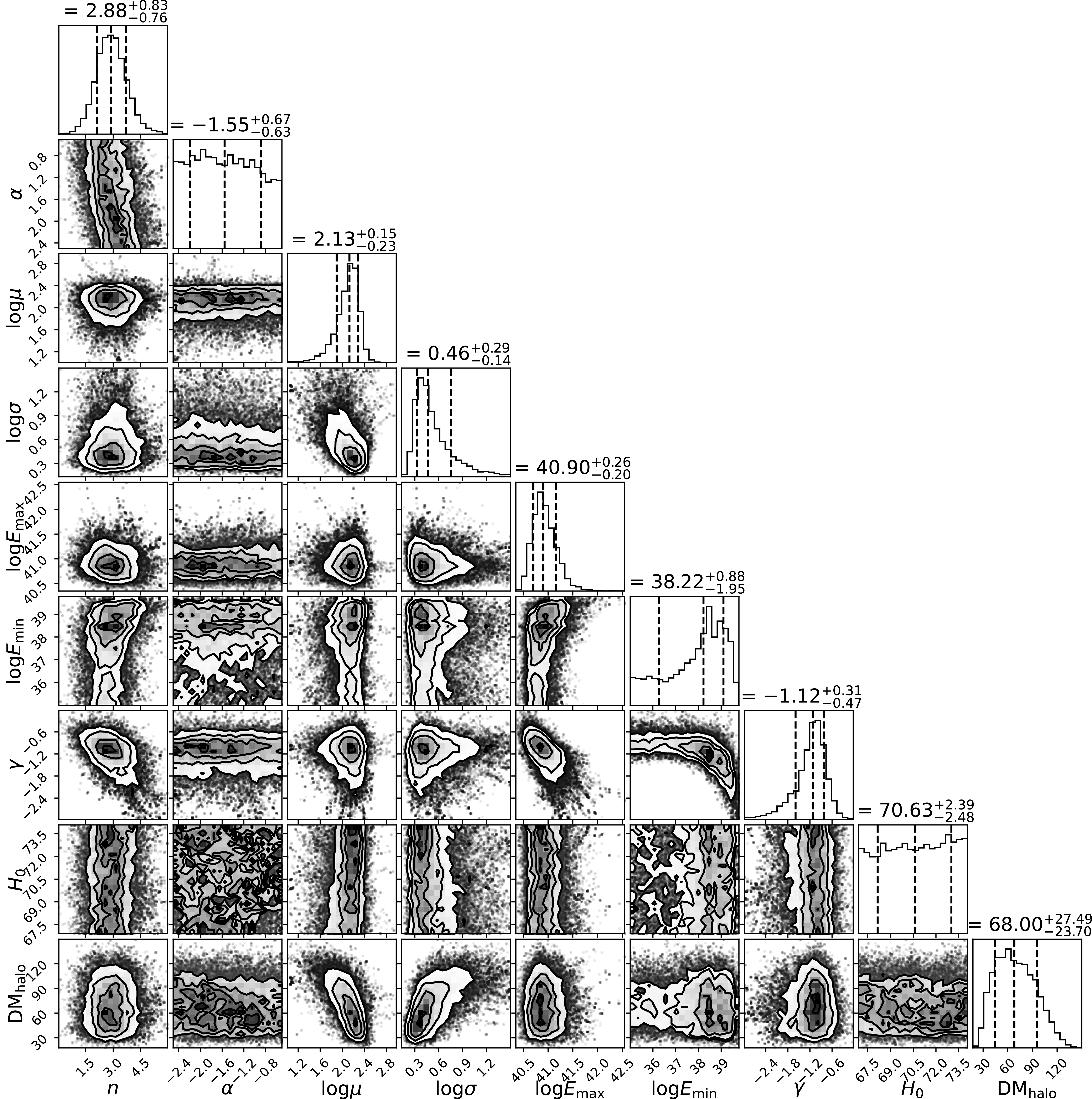
We obtain a constraint on the mean value of DM $_\mathrm{MW,halo}$
=
$_\mathrm{MW,halo}$
= $68^{+27}_{-24}$
pc cm
$68^{+27}_{-24}$
pc cm $^{-3}$
. Figure 1 shows our results for an MCMC analysis using 30 walkers, 3 000 steps and a burn-in of 500. The values for most parameters do not differ significantly from the results of Hoffmann et al. (Reference Hoffmann2025), and hence we focus our discussion here on the results of DM
$^{-3}$
. Figure 1 shows our results for an MCMC analysis using 30 walkers, 3 000 steps and a burn-in of 500. The values for most parameters do not differ significantly from the results of Hoffmann et al. (Reference Hoffmann2025), and hence we focus our discussion here on the results of DM $_\mathrm{MW,halo}$
. We note that our results for
$_\mathrm{MW,halo}$
. We note that our results for $\alpha$
and
$\alpha$
and $H_0$
are a function of the priors, and we have no constraining power within the range set by the priors, as expected from Section 2.2.
$H_0$
are a function of the priors, and we have no constraining power within the range set by the priors, as expected from Section 2.2.
3.1. DM
$_\mathrm{MW,halo}$
correlations

Figure 2 shows the correlation between DM $_\mathrm{MW,halo}$
and the host galaxy parameter
$_\mathrm{MW,halo}$
and the host galaxy parameter $\mu_\mathrm{host}$
. The orange line shows the expected relationship from Equation (1). As expected, we observe an anti-correlation between these parameters, which is also evident between DM
$\mu_\mathrm{host}$
. The orange line shows the expected relationship from Equation (1). As expected, we observe an anti-correlation between these parameters, which is also evident between DM $_\mathrm{MW,halo}$
and
$_\mathrm{MW,halo}$
and $\sigma_\mathrm{host}$
. While both DM
$\sigma_\mathrm{host}$
. While both DM $_\mathrm{MW,halo}$
and
$_\mathrm{MW,halo}$
and $\mu_\mathrm{host}$
represent a constant, average contribution to each FRB in our analysis, the degeneracy between the two parameters is broken due to the
$\mu_\mathrm{host}$
represent a constant, average contribution to each FRB in our analysis, the degeneracy between the two parameters is broken due to the $(1+z)^{-1}$
weighting factor on DM
$(1+z)^{-1}$
weighting factor on DM $_\mathrm{host}$
caused by cosmic expansion and the difference in our chosen distributions (linear-normal and log-normal, respectively) as discussed in Section 2.3.
$_\mathrm{host}$
caused by cosmic expansion and the difference in our chosen distributions (linear-normal and log-normal, respectively) as discussed in Section 2.3.
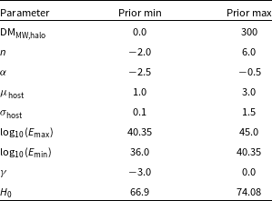
Limits on the uniform priors used. The parameters are as follows: n gives the correlation with the cosmic SFR history; $\alpha$
is the slope of the spectral dependence;
$\alpha$
is the slope of the spectral dependence; $\mu_{\mathrm{host}}$
and
$\mu_{\mathrm{host}}$
and $\sigma_{\mathrm{host}}$
are the mean and standard deviation of the assumed log-normal distribution of host galaxy DMs;
$\sigma_{\mathrm{host}}$
are the mean and standard deviation of the assumed log-normal distribution of host galaxy DMs; $E_{\mathrm{max}}$
notes the exponential cutoff of the luminosity function (modelled as a Gamma function);
$E_{\mathrm{max}}$
notes the exponential cutoff of the luminosity function (modelled as a Gamma function); $E_{\mathrm{min}}$
is a hard cutoff for the lowest FRB energy;
$E_{\mathrm{min}}$
is a hard cutoff for the lowest FRB energy; $\gamma$
is the slope of the luminosity function; and
$\gamma$
is the slope of the luminosity function; and $H_0$
is the Hubble constant. DM
$H_0$
is the Hubble constant. DM $_\mathrm{MW,halo}$
is in units of pc cm
$_\mathrm{MW,halo}$
is in units of pc cm $^{-3}$
. The host parameters
$^{-3}$
. The host parameters $\mu_{\mathrm{host}}$
and
$\mu_{\mathrm{host}}$
and $\sigma_{\mathrm{host}}$
are in units of pc cm
$\sigma_{\mathrm{host}}$
are in units of pc cm $^{-3}$
in log space,
$^{-3}$
in log space, $E_{\mathrm{max}}$
and
$E_{\mathrm{max}}$
and $E_{\mathrm{min}}$
are in units of ergs and
$E_{\mathrm{min}}$
are in units of ergs and $H_0$
is in units of km
$H_0$
is in units of km $\:\textit{s}^{-1}\:$
Mpc
$\:\textit{s}^{-1}\:$
Mpc $^{-1}$
. The limits on
$^{-1}$
. The limits on $\alpha$
were informed by existing measurements in the literature. The limits on
$\alpha$
were informed by existing measurements in the literature. The limits on $E_{\mathrm{max}}$
and
$E_{\mathrm{max}}$
and $E_{\mathrm{min}}$
were chosen as the distributions are uniform on the extrema of these ranges. The limits on
$E_{\mathrm{min}}$
were chosen as the distributions are uniform on the extrema of these ranges. The limits on $H_0$
represent a 1
$H_0$
represent a 1 $\sigma$
interval around the Planck Collaboration et al. (2020) and Riess et al. (Reference Riess2022) results.
$\sigma$
interval around the Planck Collaboration et al. (2020) and Riess et al. (Reference Riess2022) results.

Shown is the correlation between DM $_\mathrm{MW,halo}$
and
$_\mathrm{MW,halo}$
and $\mu_\mathrm{host}$
from our MCMC analysis. Overplotted in orange is the expected degeneracy, calculated according to Equation (1).
$\mu_\mathrm{host}$
from our MCMC analysis. Overplotted in orange is the expected degeneracy, calculated according to Equation (1).

We do not expect to see, and indeed do not see, strong correlations with other parameters. This confirms our previous assertions that our assumptions of DM $_\mathrm{MW,halo}$
would not have a large impact on any of our previous results with the exclusion of DM
$_\mathrm{MW,halo}$
would not have a large impact on any of our previous results with the exclusion of DM $_\mathrm{host}$
parameters.
$_\mathrm{host}$
parameters.
4. Discussion
4.1. Comparison with other results
Previously, Cook et al. (Reference Cook2023) placed an upper limit on DM $_\mathrm{MW,halo}$
of 52–111 pc cm
$_\mathrm{MW,halo}$
of 52–111 pc cm $^{-3}$
using a sample of CHIME FRBs by observing a gap in DMs between Galactic pulsars and extraGalactic FRBs. This result is in good agreement with our own result of DM
$^{-3}$
using a sample of CHIME FRBs by observing a gap in DMs between Galactic pulsars and extraGalactic FRBs. This result is in good agreement with our own result of DM $_\mathrm{MW,halo}$
=
$_\mathrm{MW,halo}$
= $68^{+27}_{-24}$
pc cm
$68^{+27}_{-24}$
pc cm $^{-3}$
, however, our results are more constraining, which is to be expected when using a larger number of localised FRBs. Ravi et al. (Reference Ravi2025) obtained a slightly lower upper limit of
$^{-3}$
, however, our results are more constraining, which is to be expected when using a larger number of localised FRBs. Ravi et al. (Reference Ravi2025) obtained a slightly lower upper limit of $47.3$
pc cm
$47.3$
pc cm $^{-3}$
using a single nearby FRB. This result is in agreement with our own within
$^{-3}$
using a single nearby FRB. This result is in agreement with our own within $1\,\sigma$
. The estimated DM
$1\,\sigma$
. The estimated DM $_\mathrm{MW,ISM}$
of this FRB exceeds the total DM of the source, which attests to the large uncertainties along this line-of-sight and hence we expect our result to be more robust.
$_\mathrm{MW,ISM}$
of this FRB exceeds the total DM of the source, which attests to the large uncertainties along this line-of-sight and hence we expect our result to be more robust.
In addition to measurements from FRBs, measurements from X-ray observations have been historically more prevalent. Prochaska & Zheng (Reference Prochaska and Zheng2019) estimated values of 50–80 pc cm $^{-3}$
using X-ray absorption lines and Yamasaki & Totani (Reference Yamasaki and Totani2020) predicted a full range of 30–245 pc cm
$^{-3}$
using X-ray absorption lines and Yamasaki & Totani (Reference Yamasaki and Totani2020) predicted a full range of 30–245 pc cm $^{-3}$
with a mean of 43 pc cm
$^{-3}$
with a mean of 43 pc cm $^{-3}$
based on X-ray emission. Das et al. (Reference Das, Mathur, Gupta, Nicastro and Krongold2021) use a combination of emission and absorption lines from numerous elements and estimate DM
$^{-3}$
based on X-ray emission. Das et al. (Reference Das, Mathur, Gupta, Nicastro and Krongold2021) use a combination of emission and absorption lines from numerous elements and estimate DM $_\mathrm{MW,halo}$
in the range of 12–1 749 pc cm
$_\mathrm{MW,halo}$
in the range of 12–1 749 pc cm $^{-3}$
with a mean and a median of 161 and 64 pc cm
$^{-3}$
with a mean and a median of 161 and 64 pc cm $^{-3}$
, respectively. X-ray absorption is preferentially biased against low densities, while DM probes all states of ionised gas. As such, it is unsurprising that results from X-ray absorption give lower predicted values. The results of Das et al. (Reference Das, Mathur, Gupta, Nicastro and Krongold2021) are in much closer agreement with our own, and these results have corrected for other states of gas that are not visible to X-ray probes.
$^{-3}$
, respectively. X-ray absorption is preferentially biased against low densities, while DM probes all states of ionised gas. As such, it is unsurprising that results from X-ray absorption give lower predicted values. The results of Das et al. (Reference Das, Mathur, Gupta, Nicastro and Krongold2021) are in much closer agreement with our own, and these results have corrected for other states of gas that are not visible to X-ray probes.
These studies give a statistical distribution of direct measurements of DM $_\mathrm{MW,halo}$
and have shown a positive skew within this distribution (see Das et al. Reference Das, Mathur, Gupta, Nicastro and Krongold2021), causing the mean values to greatly exceed the median. We similarly see a positive skew in our results. However, our results of DM
$_\mathrm{MW,halo}$
and have shown a positive skew within this distribution (see Das et al. Reference Das, Mathur, Gupta, Nicastro and Krongold2021), causing the mean values to greatly exceed the median. We similarly see a positive skew in our results. However, our results of DM $_\mathrm{MW,halo}$
represent the distribution of the mean DM
$_\mathrm{MW,halo}$
represent the distribution of the mean DM $_\mathrm{MW,halo}$
value and not an overall distribution of DM
$_\mathrm{MW,halo}$
value and not an overall distribution of DM $_\mathrm{MW,halo}$
values given by Das et al. (Reference Das, Mathur, Gupta, Nicastro and Krongold2021).
$_\mathrm{MW,halo}$
values given by Das et al. (Reference Das, Mathur, Gupta, Nicastro and Krongold2021).
The Large Magellanic Cloud (LMC) and Small Magellanic Cloud (SMC) also sit at a similar displacement from the Milky Way disk as the halo. As such, pulsars within the LMC and SMC can also inform us on the expected value for DM $_\mathrm{host}$
. Using these pulsars, Anderson & Bregman (Reference Anderson and Bregman2010) estimate a low contribution of DM
$_\mathrm{host}$
. Using these pulsars, Anderson & Bregman (Reference Anderson and Bregman2010) estimate a low contribution of DM $_\mathrm{MW,halo}$ $=23$
pc cm
$=23$
pc cm $^{-3}$
which is 2
$^{-3}$
which is 2 $\sigma$
below our estimated value. However, the exact placement and extent of the halo is unclear, and hence whether the SMC and LMC lie within the halo or not is uncertain (e.g. Ravi et al. Reference Ravi2025), meaning these measurements do not provide hard upper-limits on DM
$\sigma$
below our estimated value. However, the exact placement and extent of the halo is unclear, and hence whether the SMC and LMC lie within the halo or not is uncertain (e.g. Ravi et al. Reference Ravi2025), meaning these measurements do not provide hard upper-limits on DM $_\mathrm{MW,halo}$
.
$_\mathrm{MW,halo}$
.
4.2. Impact of single low-DM FRBs
The primary advantage that our approach has over previous studies using FRBs to constrain DM $_\mathrm{MW,halo}$
is in using an ensemble of FRBs rather than single, nearby bursts. However, it is undeniable that these low-DM FRBs provide significant constraining power on DM
$_\mathrm{MW,halo}$
is in using an ensemble of FRBs rather than single, nearby bursts. However, it is undeniable that these low-DM FRBs provide significant constraining power on DM $_\mathrm{MW,halo}$
. As such, we investigate the impact that a single FRB, such as FRB 20220319D, would have if we could get reliable DM
$_\mathrm{MW,halo}$
. As such, we investigate the impact that a single FRB, such as FRB 20220319D, would have if we could get reliable DM $_\mathrm{MW,ISM}$
estimates.
$_\mathrm{MW,ISM}$
estimates.
Of the nearby FRBs, FRB 20220319D provides the strictest constraint, and was previously used to provide an upper limit on DM $_\mathrm{MW,halo}$
of 47.3 pc cm
$_\mathrm{MW,halo}$
of 47.3 pc cm $^{-3}$
(Ravi et al. Reference Ravi2025). We have excluded this FRB from our analysis as it is at a low Galactic latitude (
$^{-3}$
(Ravi et al. Reference Ravi2025). We have excluded this FRB from our analysis as it is at a low Galactic latitude ( $b = 9.1^{\circ}$
). In fact, this FRB is a primary example of why we exclude FRBs at such low Galactic latitudes as the predicted DM
$b = 9.1^{\circ}$
). In fact, this FRB is a primary example of why we exclude FRBs at such low Galactic latitudes as the predicted DM $_\mathrm{MW,ISM}$
contribution from both NE2001 and YMW16 (Yao, Manchester, & Wang Reference Yao, Manchester and Wang2017) exceeds the total DM of the FRB, and hence are necessarily incorrect. Even with more in-depth analysis using nearby pulsar DMs, the Galactic contribution is unreliable, as even adjacent sightlines through the Galactic plane have highly varying DM values (Cordes & Lazio Reference Cordes and Lazio2002; Das et al. Reference Das, Mathur, Gupta, Nicastro and Krongold2021). However, we still show the effect of such a nearby FRB if it were to be detected out of the Galactic plane with more reliable constraints.
$_\mathrm{MW,ISM}$
contribution from both NE2001 and YMW16 (Yao, Manchester, & Wang Reference Yao, Manchester and Wang2017) exceeds the total DM of the FRB, and hence are necessarily incorrect. Even with more in-depth analysis using nearby pulsar DMs, the Galactic contribution is unreliable, as even adjacent sightlines through the Galactic plane have highly varying DM values (Cordes & Lazio Reference Cordes and Lazio2002; Das et al. Reference Das, Mathur, Gupta, Nicastro and Krongold2021). However, we still show the effect of such a nearby FRB if it were to be detected out of the Galactic plane with more reliable constraints.
Figure 3 shows our constraints on DM $_\mathrm{MW,halo}$
when keeping all other parameters fixed at their best-fit values as shown in Figure 1. The plot shows the difference of including this one FRB, with only a 20% uncertainty on DM
$_\mathrm{MW,halo}$
when keeping all other parameters fixed at their best-fit values as shown in Figure 1. The plot shows the difference of including this one FRB, with only a 20% uncertainty on DM $_\mathrm{MW,ISM}$
. When excluding this FRB we obtain DM
$_\mathrm{MW,ISM}$
. When excluding this FRB we obtain DM $_\mathrm{MW,halo}$
= 55 pc cm
$_\mathrm{MW,halo}$
= 55 pc cm $^{-3}$
and when including it this decreases to DM
$^{-3}$
and when including it this decreases to DM $_\mathrm{MW,halo}$
= 45 pc cm
$_\mathrm{MW,halo}$
= 45 pc cm $^{-3}$
. Thus, it is clear that these nearby FRBs do provide strong upper limits on DM
$^{-3}$
. Thus, it is clear that these nearby FRBs do provide strong upper limits on DM $_\mathrm{MW,halo}$
as we would expect, and detections of such FRBs outside of the Galactic plane would greatly improve our results by providing stringent upper limits.
$_\mathrm{MW,halo}$
as we would expect, and detections of such FRBs outside of the Galactic plane would greatly improve our results by providing stringent upper limits.
A slice through DM $_\mathrm{MW,halo}$
when including or excluding FRB 20220319D. All other parameters are kept constant at their best fit values from Figure 1. When excluding FRB 20220319D we obtain DM
$_\mathrm{MW,halo}$
when including or excluding FRB 20220319D. All other parameters are kept constant at their best fit values from Figure 1. When excluding FRB 20220319D we obtain DM $_\mathrm{MW,halo}$
= 55 pc cm
$_\mathrm{MW,halo}$
= 55 pc cm $^{-3}$
and when including it we obtain DM
$^{-3}$
and when including it we obtain DM $_\mathrm{MW,halo}$
= 45 pc cm
$_\mathrm{MW,halo}$
= 45 pc cm $^{-3}$
.
$^{-3}$
.

4.3. Comparing halo models
Our analysis assumes an isotropic halo, however, there has been evidence that there is structure within the Galactic halo (Yamasaki & Totani Reference Yamasaki and Totani2020; Das et al. Reference Das, Mathur, Gupta, Nicastro and Krongold2021). As such, we investigate three different halo models here by testing to see whether they reduce the scatter around the Macquart (mean $z-$
DM) relation.
$z-$
DM) relation.
The first model is our assumed model of an isotropic halo, which takes on a single average value in all directions. The second is informed by X-ray observations and implements a smooth, isotropic, spherical halo superimposed with a disk-like component (Yamasaki & Totani Reference Yamasaki and Totani2020). The third is an empirical model from Das et al. (Reference Das, Mathur, Gupta, Nicastro and Krongold2021) which uses 72 X-ray observations to map out the entire sky. This model is not smoothed and uses interpolation between nearby points to estimate the contribution for any given sight-line.
To calculate the scatter around the Macquart relation, we define $\Delta \mathrm{DM}$
as
$\Delta \mathrm{DM}$
as
 \begin{eqnarray} \Delta \mathrm{DM} &\cong& \mathrm{DM_{tot} - DM_{NE2001} - DM_{MW,halo}} \nonumber \\ && - \mathrm{DM_{Macquart}} - \frac{\langle \mathrm{DM_{host}} \rangle}{1+z}\end{eqnarray}
for each FRB, where $\langle \mathrm{DM_{host}} \rangle =$
10(
$\langle \mathrm{DM_{host}} \rangle =$
10( $\mu_\mathrm{host}$
+
$\mu_\mathrm{host}$
+ $\sigma_{\mathrm{host}}^2$
/2). A plot of this scatter for each of the models is shown in Figure 4. The corresponding median, mean, and standard deviation values are shown in Table 4.
$\sigma_{\mathrm{host}}^2$
/2). A plot of this scatter for each of the models is shown in Figure 4. The corresponding median, mean, and standard deviation values are shown in Table 4.
Residual DMs ( $\Delta \mathrm{DM}$
) of the localised FRBs used in our analysis given different halo models. This represents the scatter around the Macquart relation. The three halo models considered were an isotropic halo, an empirical halo from X-ray observations (Das et al. Reference Das, Mathur, Gupta, Nicastro and Krongold2021) and an isotropic halo with an additional disk-like component (Yamasaki & Totani Reference Yamasaki and Totani2020). The point from Das et al. (Reference Das, Mathur, Gupta, Nicastro and Krongold2021) at the bottom of the plot marked with a green cross is considered an outlier as the estimated DM
$\Delta \mathrm{DM}$
) of the localised FRBs used in our analysis given different halo models. This represents the scatter around the Macquart relation. The three halo models considered were an isotropic halo, an empirical halo from X-ray observations (Das et al. Reference Das, Mathur, Gupta, Nicastro and Krongold2021) and an isotropic halo with an additional disk-like component (Yamasaki & Totani Reference Yamasaki and Totani2020). The point from Das et al. (Reference Das, Mathur, Gupta, Nicastro and Krongold2021) at the bottom of the plot marked with a green cross is considered an outlier as the estimated DM $_\mathrm{MW}$
is
$_\mathrm{MW}$
is $1\,750^{+4\,550}_{-1\,370}$
pc cm
$1\,750^{+4\,550}_{-1\,370}$
pc cm $^{-3}$
and this estimation comes from a point 16.5 degrees away from the FRB position on the sky and hence is considered unreliable.
$^{-3}$
and this estimation comes from a point 16.5 degrees away from the FRB position on the sky and hence is considered unreliable.

The isotropic halo and the model of Yamasaki & Totani (Reference Yamasaki and Totani2020) perform very similarly with $\sigma_{\Delta \mathrm{DM}}$
values of 137 and 138 pc cm
$\sigma_{\Delta \mathrm{DM}}$
values of 137 and 138 pc cm $^{-3}$
, respectively. The fundamental difference between the models is that Yamasaki & Totani (Reference Yamasaki and Totani2020) add an extra disk-like component, which is in line with the disk of the Milky Way. However, in our analysis, we place a Galactic latitude cut on FRBs with
$^{-3}$
, respectively. The fundamental difference between the models is that Yamasaki & Totani (Reference Yamasaki and Totani2020) add an extra disk-like component, which is in line with the disk of the Milky Way. However, in our analysis, we place a Galactic latitude cut on FRBs with $|b| \lt 20^\circ$
and hence do not expect large differences between these models. The model of Das et al. (Reference Das, Mathur, Gupta, Nicastro and Krongold2021) also performs similarly with a scatter of 134 pc cm
$|b| \lt 20^\circ$
and hence do not expect large differences between these models. The model of Das et al. (Reference Das, Mathur, Gupta, Nicastro and Krongold2021) also performs similarly with a scatter of 134 pc cm $^{-3}$
. However, there is an outlier amongst the sample which, when included, increases the scatter to 324 pc cm
$^{-3}$
. However, there is an outlier amongst the sample which, when included, increases the scatter to 324 pc cm $^{-3}$
. The estimated DM
$^{-3}$
. The estimated DM $_\mathrm{MW}$
for this FRB is
$_\mathrm{MW}$
for this FRB is $1\,750^{+4\,550}_{-1\,370}$
pc cm
$1\,750^{+4\,550}_{-1\,370}$
pc cm $^{-3}$
and this estimation comes from a point 16.5 degrees away from the FRB position on the sky. As such, we choose to exclude this point from our results.
$^{-3}$
and this estimation comes from a point 16.5 degrees away from the FRB position on the sky. As such, we choose to exclude this point from our results.
Thus, we see no preference for any of the models of the Milky Way halo tested here, and would need more data to make definitive conclusions.
5. Conclusion
In this work, we use a large sample of 98 FRBs, alongside 32 associated redshifts at high ( $b\gt20^{\circ}$
) Galactic latitudes, to constrain the free electron column density in the Galactic halo. When fitting unknown FRB population parameters alongside DM
$b\gt20^{\circ}$
) Galactic latitudes, to constrain the free electron column density in the Galactic halo. When fitting unknown FRB population parameters alongside DM $_\mathrm{MW,halo}$
, we obtain a value for the mean of DM
$_\mathrm{MW,halo}$
, we obtain a value for the mean of DM $_\mathrm{MW,halo}$
=
$_\mathrm{MW,halo}$
= $68^{+27}_{-24}$
pc cm
$68^{+27}_{-24}$
pc cm $^{-3}$
, which is in good agreement with existing literature using both FRBs and X-ray observations.
$^{-3}$
, which is in good agreement with existing literature using both FRBs and X-ray observations.
Median, mean ( $\mu$
) and standard deviation (
$\mu$
) and standard deviation ( $\sigma$
) of the data from Figure 4.
$\sigma$
) of the data from Figure 4.

Our result is in good agreement with results from X-ray observations. It is higher than upper-limits provided by previous FRB studies, however, it is in agreement at the 1 $\sigma$
level. Previous studies with FRBs used a small number of low-DM FRBs in the local Universe. As such, only a single line-of-sight was considered, which may not be representative of the average contribution. However, we also find that nearby FRBs do provide strong upper limits on DM
$\sigma$
level. Previous studies with FRBs used a small number of low-DM FRBs in the local Universe. As such, only a single line-of-sight was considered, which may not be representative of the average contribution. However, we also find that nearby FRBs do provide strong upper limits on DM $_\mathrm{MW,halo}$
, and hence, if such FRBs are detected away from the Galactic plane, they would significantly improve our constraints.
$_\mathrm{MW,halo}$
, and hence, if such FRBs are detected away from the Galactic plane, they would significantly improve our constraints.
Moving forward, we expect to obtain a large number of localised FRBs in the nearby Universe from large field-of-view surveys such as CHIME and DSA. This will allow us to more robustly constrain the average value DM $_\mathrm{MW,halo}$
but also to fit the level of fluctuations in DM
$_\mathrm{MW,halo}$
but also to fit the level of fluctuations in DM $_\mathrm{MW,halo}$
which we currently select to be 15 pc cm
$_\mathrm{MW,halo}$
which we currently select to be 15 pc cm $^{-3}$
. It may also become possible to measure a distribution of DM
$^{-3}$
. It may also become possible to measure a distribution of DM $_\mathrm{MW,halo}$
values and even probe directional dependence.
$_\mathrm{MW,halo}$
values and even probe directional dependence.
Acknowledgements
This work was performed on the OzSTAR national facility at Swinburne University of Technology. The OzSTAR programme receives funding in part from the Astronomy National Collaborative Research Infrastructure Strategy (NCRIS) allocation provided by the Australian Government.
Data availability statement
The code and data used to produce our results can be found at https://github.com/FRBs/zdm.
Funding statement
This research was supported by an Australian Government Research Training Program (RTP) Scholarship. CWJ and MG acknowledge support through Australian Research Council (ARC) Discovery Project (DP) DP210102103. MG is also supported by the UK STFC Grant ST/Y001117/1. MG acknowledges support from the Inter-University Institute for Data Intensive Astronomy (IDIA). IDIA is a partnership of the University of Cape Town, the University of Pretoria and the University of the Western Cape. For the purpose of open access, the author has applied a Creative Commons Attribution (CC BY) licence to any Author Accepted Manuscript version arising from this submission.
Competing interests
None.


 Open access