



1 INTRODUCTION
The details of galaxy formation and evolution remain one of the great unsolved problem in modern astrophysics. Giant elliptical galaxies at the centre of galaxy clusters are of strong interest as they provide case studies for galaxy formation theory. On the other hand, GCs are excellent tracers of galaxy halos. Indeed, some 50% of the stars in our Galaxy may have originated in GCs (Martell & Grebel Reference Martell and Grebel2010). GCs are known to form in vigorous star formation events (Brodie & Strader Reference Brodie and Strader2006 and references therein) and were an important mode of star formation in the early universe (Muratov & Gredin Reference Muratov and Gnedin2010). It is possible that all stars may have originally formed in star clusters which are only later dispersed into the smooth stellar halos we see today (Lada & Lada Reference Lada and Lada2003). For making progress in galaxy formation theory, a holistic approach is required, which involves compositional as well as kinematical properties of GCs in giant elliptical galaxies. A landmark study (Emsellem et al. Reference Emsellem2007) suggested that a fundamental dichotomy exists between dynamically ‘slow’ and ‘fast’ rotating elliptical galaxies. These observations prompted new interpretations and theoretical models to explain this difference (Krajnovic et al. Reference Krajnovic2008; Jesseit et al. Reference Jesseit, Cappellari, Naab, Emsellem and Burkert2009). Proctor et al. (Reference Proctor, Forbes, Romanwosky, Brodie, Strader, Spolaor, Mendel and Spitler2009) suggested that the rotator class may change when the kinematics are probed beyond the inner regions.
According to various studies, classical formation of galaxies have been proposed along five major lines: (i) the monolithic collapse model, (ii) the major merger model, (iii) the multiphase dissipational collapse model, (iv) the dissipationless merger model and (v) accretion and in situ hierarchical merging. But no model is globally acceptable over others.
In this context, one is tempted to make a detailed study of an archetype of each category of elliptical galaxy. In previous papers (Chattopadhyay et al. Reference Chattopadhyay, Chattopadhyay, Davoust and Mondal2009; Chattopadhyay, Mondal, & Chattopadhyay Reference Chattopadhyay, Mondal and Chattopadhyay2013), we studied the GCs of NGC5128, which is a slowly rotating elliptical galaxy. In the present paper we study the GCs of M87, which is a strongly rotating elliptical galaxy, located at the centre of the Virgo cluster. It has a large population of GCs with well-known kinematic (Huchra & Brodie Reference Huchra and Brodie1987; Cohen & Ryzhov Reference Cohen and Ryzhov1997; Hanes et al. Reference Hanes, Cöté, Bridges, McLaughlin, Geisler, Harris, Hesser and Lee2001; Côté et al. Reference Hanes, Cöté, Bridges, McLaughlin, Geisler, Harris, Hesser and Lee2001; Strader et al. Reference Strader2011), photometric (Strom et al. Reference Strom, Strom, Wells, Forte, Smith and Harris1981; Strader et al. Reference Strader2011) and chemical properties (Mould, Oke, & Nemec Reference Mould, Oke and Nemec1987; Mould et al. Reference Mould, Oke, De Zeeuw and Nemec1990; Cohen, Blakeslee, & Ryzhov Reference Cohen, Blakeslee and Ryzhov1998). To this end, we carry out a multivariate analysis of the Lick indices, metallicities and radial distances of the GCs. First, we use independent component analysis (hereafter ICA), suitable for non-Gaussian data sets to search for the independent components (hereafter IC). The number of such components, which are linear combinations of parameters, is equal to the number of parameters (p, say). Since only a few (say, m ≪ p) of the IC components may explain a larger percentage of variation in the data, one can take only those m components instead of all p components. Then the GCs are classified on the basis of those m ICs using another exploratory data analytic method, namely K-means CA (Chattopadhyay et al. Reference Chattopadhyay, Chattopadhyay, Davoust and Mondal2009; Chattopadhyay, Sharina, & Karmakar Reference Chattopadhyay, Sharina and Karmakar2010; Chattopadhyay et al. Reference Chattopadhyay, Sharina, Davoust, De and Chattopadhyay2012; Chattopadhyay & Karmakar Reference Chattopadhyay and Karmakar2013; Chattopadhyay, Mondal, & Chattopadhyay Reference Chattopadhyay, Mondal and Chattopadhyay2013) to find the homogeneous groups. In the end, the properties of the homogeneous groups of GCs allow us to propose a possible scenario for the formation of the GCs and their host galaxy.
The data sets used are presented in Section 2. Section 3 describes different methods used in the study. The results and interpretations have been included in Section 4.
2 DATA SET
The Lick indices (Hβ, Mg1, Mg2, Mgb, Fe5270, Fe5335, NaD and TiO1) and metallicities (Fe/H) used in the present analysis were taken from Cohen et al. (Reference Cohen, Blakeslee and Ryzhov1998). From the original sample of 150 GCs we removed the GCs with identification numbers 5024 and 5026, because they are redundant with 978 (Hanes et al. Reference Hanes, Cöté, Bridges, McLaughlin, Geisler, Harris, Hesser and Lee2001), as well as 321 which is a star (Strader et al. Reference Strader2011), thus reducing the sample to 147 GCs. In the latter paper, the identification number given by Cohen et al. (Reference Cohen, Blakeslee and Ryzhov1998) is preceded by ‘S’. The velocities  $v_{\text{rad}}$, half-light radii rh, i magnitudes ( $i_{\text{mag}}$) and (g − r) and (g − i) colours were taken from Strader et al. (Reference Strader2011). The radial distances R and position angles ψ were derived from the coordinates listed in Strader et al. (Reference Strader2011), assuming that the centre of the system of GCs is also that of the galaxy, which is at αc = 12 h 30 m 49.42 s and δc = 12d 23′ 28.044″ (Lambert & Gontier Reference Lambert and Gontier2009).
It is to be noted that our sample size is small compared to the recently observed samples by various authors (e.g. Strader et al. Reference Strader2011). We have thus plotted the histograms of i-magnitudes and radial distances of our sample and have compared with the sample used by Strader et al. (Reference Strader2011) (Figure 1). Now Strader et al. (Reference Strader2011) have found that the bright and faint GCs have the same velocity dispersions (sigma = 340 and 339 kms−1). In their Section 6.3.4, they find that there is no strong trend with magnitude for the red GCs. For the blue GCs, there is perhaps an avoidance of the systematic velocity, although marginal. The conclusion is that the bright and faint compact blue GCs belong to the same population. So we can safely say that, if the kinematics are an indicator of the origin of GCs, then our sample should be enough to determine the origin of the inner GCs.
Comparison of the histograms of i mag and R of the GCs of our sample (red solid line) and the sample of Strader et al. (Reference Strader2011) (black solid line).

For comparison purposes, we used the Lick indices of 313 old clusters in M31 (Schiavon et al. Reference Schiavon, Caldwell, Morrison, Harding, Courteau, MacArthur and Graves2012), those of 47 GCs in 4472 (Cohen, Blakeslee, & Côté Reference Cohen, Blakeslee and Côté2003) and 33 GCs in NGC 4636 (Park et al. Reference Park, Lee, Hwang, Kim, Arimoto, Yamada, Tamura and Onodera2012).
3 STATISTICAL METHODS
3.1. Shapiro–Wilk test
The choice of statistical methods to apply to a set of data depends on its Gaussian or non-Gaussian nature. We have thus tested the Gaussianity of our data set by the Shapiro–Wilk test (Reference Shapiro and Wilk1965). According to this test, the null hypothesis is that the data set is Gaussian. The test statistic W is defined as W = Σni = 1aix 2i/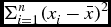 $\Sigma _{i=1}^n (x_i -\bar{x})^2$ where n is the number of observations, xi are the ordered sample values and ai are constants generated from means, variances, and covariances of the order statistics of a sample of size n from a normal distribution. In our case the data set is multivariate, hence we have used the multivariate extension of the Shapiro–Wilk test. We found that the p value of the test is 1.327 × 10⁻¹¹, which is very small. Thus, the null hypothesis is rejected at a 5% level of significance. We conclude that the present data set is non-Gaussian in nature.
3.2. Independent component analysis
While Principal Component Analysis (PCA) applies to Gaussian data sets, ICA applies to non-Gaussian data sets. ICA is a dimension reduction technique, i.e. it reduces the number of observable parameters p to a number m (m ≪ p) of new parameters, where these new parameters are the linear combinations of p parameters, such that these m parameters are mutually independent. Mathematically speaking, let X 1, X 2, . . ., Xp be p random vectors (here p parameters) and n (here 147) be the number of observations of each Xi (i = 1,2,. . .,p).
Let
 $$\begin{equation}
X = AS,
\end{equation}$$
$$\begin{equation}
X = AS,
\end{equation}$$
where S = [S 1, S 2, . . ., Sp]′ is a random vector of hidden components Si (i = 1,2,. . .,n) such that Si are mutually independent and A is a non-singular matrix. The goal of ICA is to estimate A and to find S by inverting A, i.e.
 $$\begin{equation}
S = A^{-1} X \ \quad \text{i.e.} \ \ S = WX.
\end{equation}$$
$$\begin{equation}
S = A^{-1} X \ \quad \text{i.e.} \ \ S = WX.
\end{equation}$$
Under ICA, we find the components [S 1, S 2, . . ., Sn] those are independent by finding an unmixing matrix W in such a way that the covariance between any two nonlinear functions g 1(Si) and g 2(Sj) for i ≠ j is zero i.e. the ICs are nonlinearly uncorrelated (for more details, see Comon (Reference Comon1994); Chattopadhyay Mondal, & Chattopadhyay, (Reference Chattopadhyay, Mondal and Chattopadhyay2013) and references therein).
At present, there is no better method available to automatically determine the optimum number of ICs. In this paper, the number of ICs is determined by the number of Principal Components (PCs) chosen (Albazzaz and Wang, Reference Albazzaz and Wang2004). To reduce the number of components Si from p to m (m ≪ p), one is to perform PCA (Babu et al. Reference Babu, Chattopadhyay, Chattopadhyay and Mondal2009; Chattopadhyay & Chattopadhyay Reference Chattopadhyay and Chattopadhyay2007; Fraix-Burnet et al. Reference Fraix-Burnet, Chattopadhyay, Chattopadhyay and Davoust2010; Chattopadhyay et al. Reference Chattopadhyay, Sharina and Karmakar2010). In this method also Yi’s (i = 1,2,. . .,p) vectors are found, which are linear combinations of Xi’s (i = 1,2,. . .,p) such that Yi’s are uncorrelated. The number of (initially p) components is reduced to m by taking those Yi’s (i = 1,2. . .,m) for which the corresponding eigenvalues λi ~ 1.
In the present work, we have first performed PCA to find the significant number of IC components to be chosen. PCA applies to Gaussian data, but the present data set is non-Gaussian, so we performed ICA. In PCA, the maximum variation with significantly high eigenvalue (viz. λ ~ 1) was found to be almost 78% for three PCA components. Hence, we have chosen three IC components for the CA. The parameters chosen for ICA are the Lick indices Hβ, Mg1, Mg2, Mgb, Fe5270, Fe5335, NaD, TiO, the metallicity Fe/H, the photometric parameters magnitude  $i_{\text{mag}}$ and colours (g − r), (g − i) and the projected galactocentric distance R (in arcsec).
3.3. K-means cluster analysis
K-means CA is a multivariate technique for finding homogeneous groups in a data set giving information of the underlying structure in this data set. In this method one finds k groups, provided each group contains an object and each object belongs to exactly one group. Hence, the maximum and minimum number of possible groups are k = n and k = 1, respectively. The algorithm is as follows :
(i) All the objects are divided into k (given) groups in a random manner.
(ii) Any group is selected and any particular object of that group is taken first. Then the parametric distance (here the parameters are three IC components) from the chosen object is computed for the remaining objects. If the distance between objects in the group is greater than that for objects in other groups, they are interchanged.
(iii) Process (ii) is applied for all objects and for all groups.
(iv) Steps (i) and (iii) are continued until there is no further change.
The k groups thus found are coherent in nature.
The optimum value of k is found as follows. First one finds groups for k = 1, 2, 3,. . .etc. Then a distance measure  $\text{d}_k$ is computed by
 $$\begin{equation}
\text{d}_k=(1/p)\text{min}_x\;E[(x_k-c_k)^{\prime }(x_k-c_k)],
\end{equation}$$
$$\begin{equation}
\text{d}_k=(1/p)\text{min}_x\;E[(x_k-c_k)^{\prime }(x_k-c_k)],
\end{equation}$$
which is the distance of xk vector (values of parameters) from the centroid ck of the corresponding group. The optimum value of k is that for which  $J_k = (\text{d}_k^{^{\prime } -p/2}-\text{d}_{k-1}^{^{\prime } -p/2})$, is maximum (Sugar & James Reference Sugar and James2003). In the present case, k = 4.
For CA, the number of parameters are three IC components chosen as previously described. The optimum number of groups is selected objectively by k-means clustering (MacQueen Reference MacQueen, Lecom and Neyman1967), together with the method developed by Sugar and James (Reference Sugar and James2003). The optimum number is k = 4. The groups are labelled G1, G2, G3, and G4.
For testing the robustness of the classification, we have proceeded in the following manner. In the original scheme, the number of parameters is 13. First, we have constructed the variance covariance matrix of the parameters and selected the parameters having maximum variances e.g. here H β, Mgb, Fe5270, Fe5335, NaD, Fe/H,  $i_{\text{mag}}$, R have variances greater than 0.25 and the remaining ones, Mg1, Mg2, TiO1, g − r, g − i have variances ~ 0.0. Therefore, we have done the analysis with the above eight parameters and have obtained exactly the same groups with no variation at all. So, we can at once say that our classification is robust with respect to the parameters which are responsible for the maximum variation.
Regarding the uncertainties on the various parameters, the method we have used is totally exploratory (i.e. no underlying distribution is assumed). Hence, it is not possible to see the effect of error in such type of analysis directly. What we can do at most is to change the values of the parameters within the range permitted by the error bars and redo the analysis. We have tested it for that for few values of the parameters and found the same groups. Alternatively, once the optimum classification (clustering) is obtained, one can use a process called discriminant analysis (Johnson & Wichern Reference Johnson and Wichern1998) to verify the acceptability of the classification of different GCs. In this standard procedure, using the probability density functions in parameter space for the different clusters, one can assign an object (in this case, a GC) to be a member of a certain class. If the original classification is robust, then every GC should be classified again as a member of the same class that it was before. If a significant number of objects are not reclassified then that means that the original classification is not stable and hence not trustworthy. Table 1 shows the result of a discriminant analysis, where the columns represent how the GCs of a cluster were assigned by the analysis. The fraction of correct classifications is 0.925, which implies that the classification is indeed robust by computing classification/misclassification probabilities for the GCs.
Discriminant analysis for K-means classification: G1, G2, G3, and G4 are groups found by K-means cluster analysis and G1*, G2*, G3*, and G4* are groups found by discriminant analysis.

3.4. Levenberg–Marquardt Algorithm
This algorithm is used to find the most probable mean rotation curve for each group, assuming that they have a solid-body rotation around the centre of the galaxy. This is a reasonable assumption for the two innermost groups, G1 and G4, because the galaxy itself is in solid-body rotation at least to a radius of 225 arcsec (Cohen & Ryzhov, Reference Cohen and Ryzhov1997). For the two other groups, G2 and G3, we also tried a rotation curve that flattens beyond 225 arcsec, but the data were better adjusted by a solid-body rotation curve (also see Figure 7 of Kissler-Patig & Gebhardt Reference Kissler-Patig and Gebhardt1998).
The rotation amplitudes  $v_{\text{rot}}$ (= ΩR) and the position angles (ψ0) of the axes of rotation (East to North) of the different groups G1–G4, (found in the CA) are computed by the relation
 $$\begin{equation}
v_{\text{rad}}(\psi )=v_{\text{sys}}+\Omega R\sin (\psi -\psi _0),
\end{equation}$$
$$\begin{equation}
v_{\text{rad}}(\psi )=v_{\text{sys}}+\Omega R\sin (\psi -\psi _0),
\end{equation}$$
(Côté et al. Reference Côté2001; Richtler et al. Reference Richtler2004; Woodley et al. Reference Woodley, Harris, Beasley, Peng, Bridges, Forbes and Harris2007), where vr is the observed radial velocity,  $v_{\text{sys}}$ is taken as the recession velocity of the galaxy, which is 1287 km s−1.Footnote 1R is the projected distance of each GC and ψ is its position angle, measured East to North. We have used Levenberg–Marquardt fitting method (Levenberg Reference Levenberg1944; Marquardt Reference Marquardt1963) to solve for $v_{\text{rot}}$ and ψ0. They are listed in Table 2 for G1–G4. Now kinematic data sets for G1–G4 are small and for such situation Monte Carlo simulations are used to increase the data sets to have a more convincing result. Monte Carlo simulation needs distributional assumption and here no well known bivariate distribution is fitting with the data well. So, we have taken several bootstrap samples and have computed the mean values with standard errors of the rotation parameters. The errors are small as seen from Table 2.
Mean values of various parameters of G1–G4 together with kinematics.

4 RESULTS AND INTERPRETATION
4.1. Properties of globular clusters in the four groups
The CA divided the GCs of M87 into four groups. We did not use the kinematical data ( $v_{\text{rad}}$ and ψ) in the statistical analysis. Nor did we use Mgb/Fe. The latter is an indicator of the abundance in light elements. But we did use these parameters for interpreting the results.
The results of the analysis are summarised in Table 2, which lists the mean values of all the parameters with standard errors for the four groups. The mean velocities of rotation and mean position angles have been computed by the Levenberg–Marquardt algorithm.
To show how the groups are separated, we have plotted three ICs (viz. IC1, IC2 and IC3) for the groups G1–G4 found in our analysis (Figure 2). That figure shows that the groups are well separated in IC space.
Plot of IC1, IC2, and IC3 of G1(blue circles), G2(red circles), G3(green circles), and G4 (black circles) groups of GCs.
We first investigate how the different groups differ in their Lick index values, and how they compare in this respect with the simple stellar population models of Thomas, Maraston, & Johansson (Reference Thomas, Maraston and Johansson2011). As shown in Figures 3–5, G3 has the lowest values of Fe5270, NaD,TiO, and Mgb, while G4 has the highest values of these Lick indices, and G1 and G2 are in between. These two latter groups differ in that G1 is marginally less chemically evolved than G2 (these two groups also differ in their spatial distribution and in their kinematics). In other words, the order of increasing overall chemical evolution is G3, G1, G2, and G4. The Lick index Hβ is an age indicator, higher values meaning younger ages, but this index is also sensitive to the colour of the Horizontal Branch (HB), higher values meaning a bluer HB. A bluer HB in turn can be due to He-enriched stars. So the interpretation of Figure 6, which shows the run of Hβ versus Mgb, is best done with the help of stellar population models, namely those of Thomas et al. (Reference Thomas, Maraston and Johansson2011). The data are well fit by models of 12 Gyr, albeit with a large scatter suggesting a variety of HBs and/or of α/Fe. An alternative explanation in terms of stellar populations with younger ages is not possible because it would not be compatible with the observed broad-band colours (see below).
Fe 5270 versus Mgb for G1–G4. Blue open squares for G1, red open squares for G2, green open squares for G3, black open squares for G4, cyan filled squares for GCs of M31. Black lines are stellar population models of Thomas et al.(Reference Thomas, Maraston and Johansson2011) for an age of 12 Gyr, a dotted line for α/Fe = − 0.3 and solid lines are for α/Fe = 0.0, 0.3, and 0.5 respectively from left to right.
NaD versus Mgb for G1–G4 and for GCs of M31 (small cyan squares), NGC4472 (small magenta squares), NGC4636 (small black squares). The colours and symbols are the same as in Figure 3. NaD is higher in the GCs of the spiral galaxy than in those of the elliptical galaxies.
TiO1 versus Mgb for G1–G4 along with GCs of M31 and NGC4472. The colours and symbols are the same as in Figure 4. TiO1 is higher in the GCs of the spiral galaxy than in those of the elliptical galaxies.
Hβ vesus Mgb for G1–G4. The colours and symbols are same as in Figure 4. The large spread in Hβ in G1–G4 can be due to a spread in α/Fe and/or in colour of the Horizontal Branch.
We next investigate the colours of the stellar populations in the GCs of M87. The colour–colour diagram for the different groups is shown in Figure 7. There is a progressive reddening of the populations, from G3 (green) to G1 (blue) followed by G2 (red) and G4 (black). This is predicted by models of synthetic stellar populations as a result of increasing age and/or metallicity. Since the models of Thomas et al. (Reference Thomas, Maraston and Johansson2011) do not predict the evolution of broad-band colours, we adjusted Yonsei models of simple stellar populations (Chung et al. Reference Chung, Lee, Yoon and Lee2013) to the data (Figure 8). The models for metallicities ranging from [Fe/H] = − 2.6 to 0.6, an age of 12 Gyr and α/Fe = 0.3 are shown as solid lines, green and blue for 0 and 70% secondary populations respectively. Changing α/Fe will only shift the model down diagonally on the figure, and changing the initial mass function has little effect on the models (see Chung et al. Reference Chung, Lee, Yoon and Lee2013). The comparison of our data to the Galev models (Kotulla et al. Reference Kotulla, Fritze, Weilbacher and Anders2009), and to the models of Maratson et al. (Reference Maratson, Greggiol, Renzini, Ortolani, Saglia, Puzia and Kissler-Patig2003) gave results (not shown) very close to those of the Yonsei model for 0% secondary populations. For the Maraston models, we converted the CFH-Megcam magnitudes to SDSS using the paper by Betoule et al. (Reference Betoule2013).
(g − i) versus (g − r) for G1–G4. The colours and symbols are the same as in Figure 3. The green and blue solid lines are Yonsei models for an age of 12 Gyr, and for 0 and 70% secondary stellar populations respectively.
[Fe/H] versus (g − i) for G1–G4. The colours and symbols are same as that for Figure 3. The green and blue lines are Yonsei stellar population models (Chung et al. Reference Chung, Lee, Yoon and Lee2013) for an age of 12 Gyr and 0 and 70% He enhanced secondary populations respectively.
The colours of the metal-poor GCs (shown on Figure 7) are well fit by the models. On the other hand, the metal-intermediate (G1) and metal-rich (G2) GCs can only be explained by a Helium-enriched secondary stellar population (Chung et al. Reference Chung, Lee, Yoon and Lee2013). No Yonsei model population with a realistic age is able to account for the colours of group G4. We have no explanation for the colours of this group, other than that they are unusual. It is not possible to advocate younger stellar populations instead of He-enriched ones to interpret the colours of the groups, because such populations are bluer in both colours, but more so in (g − i). Further evidence for He enhancement in the metal-intermediate and metal-rich GCs of M87 is the far ultraviolet excess detected in the GCs of M87 by Sohn et al. (Reference Sohn, O’Connell, Kundu, Landsman, Burstein, Bohlin, Frogel and Rose2006), an excess which increases with metallicity. Kaviraj et al. (Reference Kaviraj, Sohn, O’Connell, Yoon, Lee and Yi2007) interpret this excess by the possible presence of hot HB stars from super-He-rich stellar populations, even though their predicted ages are unrealistically old.
We next compare the properties of the GCs of M87 with those of other galaxies. The GCs of M87 have values of Fe5270 and Hβ at a given Mgb (see Figures 3 and 6) that are comparable to those of M31, but generally lower values of NaD and TiO at a given Mgb (see Figures 4 and 5), except G4. In the latter two figures, the predictions of the simple stellar population models seem to hold the middle ground between the GCs of M87 and of M31. Concerning NaD, the high values observed in M31 might be partly due to interstellar absorption and thus less reliable. We are indebted to the referee for this remark. To better understand the significance of these lower values, we also plotted the same data for GCs of two other elliptical galaxies in Virgo, NGC 4472 and 4636 on Figures 4 and 5. The GCs of these two other ellipticals show the same behaviour as those of M87, suggesting that GCs in elliptical galaxies are different from those of spirals in this respect, except at very high metallicities. We speculate that Na is underabundant in G1–G3 and that the Na − O anti-correlation present in Galactic GCs, interpreted as a result of multiple stellar populations, is only present in G4.
The abundance of light elements tends to decrease with increasing metallicity in the GCs of our Galaxy (Fraix-Burnet, Davoust & Charbonnel Reference Fraix-Burnet, Davoust and Charbonnel2009), M31 (Colucci et al. Reference Colucci, Bernstein, Cameron and McWilliam2012a), and the LMC (Colucci, Bernstein, & Cohen Reference Colucci, Bernstein and Cohen2012b), as expected from arguments of nucleosynthesis. High values of α/Fe result from star formation that occurs before type 1a supernovae significantly increase the abundance of Fe in the interstellar medium, and are expected mainly in metal-poor environments. In M87, we find that the opposite is true. We use Mgb/Fe = 2 Mgb/(Fe5270 + Fe5335) as an indicator of α/Fe and calibrate this indicator with the stellar population models of Thomas et al. (Reference Thomas, Maraston and Johansson2011). As shown on Figure 9, the light-element abundance increases with metallicity. For G1 and G2 it increases from 0 to 0.3, and for G4 it is about 0.4. For G3, which is very metal-poor, the disagreement between α/Fe and its indicator Mgb/Fe suggests that the light-element ratio estimates, which are more uncertain at low metallicity, are just not reliable for this group, which is ignored. The contrast between the GCs of M87 and those of our Galaxy and M31 in this respect are further evidence that GCs of elliptical and spiral galaxies have different chemical histories.
Fe/H versus light-element abundance indicator Mgb/Fe for G1–G4. The colours and symbols are same as in Figure 3. The blue, red, and black lines are stellar populations of Thomas et al. (Reference Thomas, Maraston and Johansson2011) for α/Fe = 0.0, 0.3, and 0.5 respectively. α/Fe increases with metallicity in G1, G2, and G4, while in G3 it has a peculiar behaviour.
We have adjusted a mean rotation curve to each of the four groups (see Section 3.4). The resulting parameters are listed in Table 2, and the mean rotation curves of the four groups along with radial velocities of the GCs are shown in Figure 10. The only groups with clear evidence of rotation are G2 and G4. The outer (radius > 300 arcsec) clusters of the group G2 rotate faster than the inner ones. Schuberth et al. (Reference Schuberth, Richtler, Hilker, Dirsch, Bassino, Romanowsky and Infante2010) have found that the metal poor GCs in the outer region of NGC 1399 (the non-rotating giant elliptical galaxy in the centre of the Fornax cluster) is the only GC population that shows significant rotation. The difference with M87 is that G2 is not the metal poorest group. There is marginal evidence for rotation in G1, about an axis which is orthogonal to that of G2. There is also evidence for rotation in G4, whose spatial distribution is flattened in the plane of rotation (along position angles of maximum or minimum radial velocity; see Figure 10). As G4 is centrally concentrated, it is worth mentioning the recent study of Emsellem et al. (Reference Emsellem2007), who find a counter-rotating core in the central 2 arcsec of M87, in position angle 20 degrees. In a detailed kinematic study of the GCs of M87, Strader et al. (Reference Strader2011) have found subpopulations with distinct kinematical behaviours, and concluded that M87 is still in active assembly. They also warned that the old kinematical data (which include the present ones) predict a higher rotation than their new data. Our own kinematical results should thus be viewed with caution. $v_{\text{rad}}$ versus PA with fitted mean rotation curves for G1–G4. In the box for G2, the red open squares are for $R \le 300\ \text{arcsec}$ and the red full squares are for $R > 300\ \text{arcsec}$. The outer GCs of that group rotate faster than the inner GCs
4.2. Origin of the four groups
The first stage of formation of a galaxy is a dissipative collapse. During that phase, chemical enrichment is expected to be accompanied by spin up of the metal-richer material which ends up in circular orbits, whereas the metal-poor material is in eccentric orbits (Eggen, Lynden-Bell, & Sandage Reference Eggen, Lynden-Bell and Sandage1962). The formation of G3 and G4 can be associated to that phase : G3 in the outer parts from metal-poor material, G4 in the inner part from metal-rich material. The lack of rotation in G3, the flattened spatial distribution, strong rotation and high average α/Fe in G4, are properties consistent with this assumption. Montes et al. (Reference Montes, Trujillo, Prieto and Acosta-Pulido2014a) have shown that the central part of M87 is super solar and presumably formed first during the monolithic collapse of the galaxy.
Montes et al. (Reference Montes, Trujillo, Prieto and Acosta-Pulido2014b) have found that the innermost GCs of M87 (within 30 arcsec) are metal poorer than the stars in the region. We show that there are actually two populations of GCs (G3 and G4) near the centre, one of solar metallicity like the stars of the central region (Montes et al. Reference Montes, Trujillo, Prieto and Acosta-Pulido2014a).
In the second stage of formation, the galaxy accretes low-mass satellites in a dissipationless fashion (Bekki & Chiba Reference Bekki and Chiba2005). The GCs of G1 and G2 may have formed in this phase. The difference between G1 and G2 could be one of time, G2 forming first and retaining the angular momentum of the gas from which it formed and G1 forming later from cooling flows close to the centre, the gas having lost its angular momentum to collision with gas clouds (viz. Table 2,  $v_{\text{rot}}$). This would explain why the GCs of G1, near the centre, have little rotation, while those of G2, in the outer regions, rotate significantly. In this scenario, one thus expects the velocity of rotation to increase outward, which seems to be the case for the GCs of G2 : $v_{\text{rot}}\sim$ 374.93 km s−1 for R ⩾ 300, and $v_{\text{rot}}\sim$ 179.92 km s−1) for R < 300.
5 CONCLUSION
We have performed a multivariate analysis of the chemical and photometric properties of the GCs of M87, and found four groups of clusters with distinct properties. The latter are used to propose a formation scenario for the different groups, in terms of dissipational collapse of the galaxy, followed by dissipationless accretion of matter.
Regardless of the clustering results, the reanalysis of data from the literature with recent stellar population models, those of Thomas et al. (Reference Thomas, Maraston and Johansson2011) and the Yonsei models (Chung et al. Reference Chung, Lee, Yoon and Lee2013), provides new insights into the chemical properties of the GCs of M87, compared to those of other galaxies. We have found that these properties are different from those of GCs in M31, in that the Lick indices NaD and TiO1 are higher at a given Mgb. We have also found a progressive excess blueing of the GCs with metallicity, which we interpret by the presence of an extreme blue HB, possibly due to He enriched secondary stellar populations. Finally, α/Fe increases with metallicity, at variance with what occurs in GCs of spiral galaxies (our own and M31). Our interpretation is one among many others and remains speculative in view of the smallness of the sample and is not an ambitious as is needed. Our interpretation is only one possible way of understanding the results.
ACKNOWLEDGEMENTS
We thank C. Chung for sending us tables for the Yonsei Evolutionary Population Synthesis models. We are also thankful to A.K.Chattopadhyay for useful discussions, and to Saptarshi Mondal for helping in some calculations. One of the authors (Tanuka Chattopadhyay) thanks DST, India for providing her a major research project for the work.



