


1. Introduction
Monetary policy has experienced an astonishing evolution in recent years. Aggressive easing policies following the unprecedented pandemic crisis of 2020–21 were soon pivoted to aggressive tightening in response to inflationary pressures escalated by supply chain disruptions, geopolitical risks, and pent-up demand. More recently, as concerns about inflation have gradually been supplanted by worries about economic downturn, monetary policy has entered a new phase. The rapid transformation of monetary policy brought renewed attention to the policy announcements issued by central banks and the information embedded within them, calling for the need for a more accurate measurement of policy shocks.
However, measuring policy shocks has become more challenging than before. As monetary policy adapts to rapidly changing economic conditions, its primary goals and associated operations have become increasingly intricate. Policy shocks, therefore, are likely to be confounded with other information pertaining to economic and financial conditions. For instance, with conventional policies constrained by the zero lower bound, major central banks’ reliance on unconventional policy measures has substantially risen, further complicating the interpretation of information in the policy shocks. Hence, policy shocks measured in a conventional manner, which typically disregards multifaceted information they contain, may yield biased results.Footnote 1
In this vein, recent literature has put emphasis on the importance of disentangling the information content within policy announcements, gauged by high-frequency fluctuations in short-term interest rates (Nakamura and Steinsson, Reference Nakamura and Steinsson2018; Jarociński and Karadi, Reference Jarociński and Karadi2020; Cieslak and Pang, Reference Cieslak and Pang2021; Bu et al. Reference Bu, Rogers and Wu2021, among many others). Among such endeavors, Jarociński and Karadi (Reference Jarociński and Karadi2020) propose a straightforward and effective method for distinguishing between pure monetary policy shocks (MP shocks, hereafter) and central bank information shocks (CBI shocks). Their approach analyzes the co-movements between interest rates and stock prices in a narrow window around policy releases. Specifically, monetary policy shocks are identified when changes in interest rates around policy announcements (monetary policy surprises) negatively co-vary with those in stock prices (stock price surprises); conversely, information shocks are obtained when the two high-frequency changes positively co-vary. A CBI shock, however, would induce the opposite-signed reaction of stock market prices, or an increase in stock prices.Footnote 2
Adopting approaches similar to Jarociński and Karadi (Reference Jarociński and Karadi2020), a burgeoning literature documents new findings regarding the impacts of the two distinct shocks. Less attention, however, has been paid to what information content is really in the two shocks identified from stock price surprises and what they reflect. Furthermore, our understanding on the strainer used to distill the shocks from monetary policy surprises is still quite limited.Footnote 3
Expanding upon the research by Jarociński and Karadi (Reference Jarociński and Karadi2020), this paper seeks to fill the gaps by addressing the following questions:
-
• What additional instruments could be considered to capture the information conveyed by policy announcements?
-
• How do monetary policy shocks and CBI shocks, sorted out by other instruments, differ from (or resemble) the benchmark counterparts by Jarociński and Karadi (Reference Jarociński and Karadi2020)? What are their impacts on the economy and financial market?
-
• From them, what insights can be gleaned about the natures of the benchmark shocks?
To answer these questions, we first compile a range of candidates for the two shocks, which are deconstructed from monetary policy surprises using alternative instruments. The instruments are chosen based on related literature, which may potentially have distinct relationships with those shocks. A total of 13 instruments are drawn from four categories: (i) New Keynesian-based (r-star and inflation expectations), (ii) Fama–French factor-based (high-minus-low (HML) and small-minus-big (SMB)), (iii) risk appetite-based (risk aversion, excess bond premium, credit spread, and VIX), and (iv) commodity- and currency-based instruments (WTI crude oil prices and various exchange rates). Next, to identify the sets of shocks, sign restrictions between each instrument and monetary policy surprises are imposed based on the theory-consistent relationships in a VAR framework. We then iteratively examine the impulse responses of economic and financial variables to the two orthogonal shocks decomposed using various sources. In particular, the responses from alternatively identified shocks are compared in parallel with those from the benchmark shocks proposed by Jarociński and Karadi (Reference Jarociński and Karadi2020). Finally, a battery of exogeneity regressions are estimated, which compare the identified candidate shocks with benchmark shocks or other structural shocks, including financial shocks, growth shocks, and uncertainty.
We establish three main findings. First, from the perspectives of dynamic consequences, Fama–French HML strongly reveals its potential as a promising instrument for sorting out the informational content in the Fed’s policy announcements. The two shocks deconstructed by HML produce the impulse responses of economic and financial variables, aligning with related theories and also with the benchmark. In particular, on a CBI shock identified with HML factor, output and prices increase, implying expansionary impacts on the real economy. In addition, stock prices and market interest rates rise after the shock, while the excess bond premium (EBP) declines at impact, reflecting easing financial conditions. Meanwhile, in response to an MP shock identified through HML, output and price fall. Also, the S&P 500 index and the one-year treasury bond yields decrease, whereas the EBP increases after the shock, indicating a contractionary effect of the shock.
Second, the remaining candidate instruments could only partially discern the information embedded in the policy announcements, as the responses of variables to their corresponding shocks deviate to some extent from what theory predicts. For instance, the shocks decomposed via r-star generate overall similar response patterns, yet with significantly larger magnitudes or insignificance. Also, the reactions of baseline variables to the shocks identified through risk aversion index (Bekaert et al. Reference Bekaert, Engstrom and Xu2021) are quite consistent with those to the benchmark shocks. However, the responses of yield curves, including long-term interest rates (10-year treasury yields) and term spread (10-year minus 2-year rates), are noticeably different from our prediction.
Third, the majority of shocks identified using alternative instruments are positively correlated with the benchmark shocks, yet convey somewhat distinct information. Specifically, the CBI shocks identified through alternative instruments demonstrate low correlations with the benchmark counterparts, albeit all being positive (average of 0.38). In the company of them, HML-based CBI shocks display a relatively high correlation (0.57) with the benchmark. Unlike CBI shocks, candidate MP shocks show relatively higher correlations with the benchmark, with an average of around 0.61. Again, that obtained using HML factor record a quite high correlation with the benchmark shock. The results from exogeneity tests provide similar conclusions. They reveal that some candidates exhibit significant correlations with other structural shocks, which are attributable to discrepancies in impulse responses, compared with stylized ones. The tests also provide reaffirming results that HML-based shocks are the closest alternative to the benchmark shocks.
Our primary contributions to the literature are twofold. First, this paper substantially expands upon the findings of a growing literature that distinguishes CBI shocks from conventional MP shocks. A seminal paper by Romer and Romer (Reference Romer and Romer2000) finds that the public may learn about the Fed’s forecasts, which are formed by processing common information more effectively than the public and by observing the Fed’s policy actions. Related literature also empirically examines and corroborates the existence of such private information held by central banks about the economy, which the public do not have (e.g., Campbell et al. Reference Campbell, Evans, Fisher, Justiniano, Calomiris and Woodford2012; Lakdawala, Reference Lakdawala2019; Lakdawala and Schaffer, Reference Lakdawala and Schaffer2019; Kerssenfischer, Reference Kerssenfischer2022; Nakamura and Steinsson, Reference Nakamura and Steinsson2018). Going forward from them, we delve deeper into the nature of the two identified shocks by comparing the results from the benchmark identification with those from alternative identifications.
Second, to our investigation, our work is the first to systematically assemble and compare the two components in monetary policy surprises, which are deconstructed using various alternative instruments. As pioneered by Jarociński and Karadi (Reference Jarociński and Karadi2020), information processing capabilities of financial markets, such as high-frequency stock price surprises, have been highlighted as a tool for distinguishing the two shocks. However, there could exist other promising instruments beside aggregate stock prices (e.g., the S&P 500 index) which are also suitable to scissor the distinct shocks (e.g., Andrade and Ferroni, Reference Andrade and Ferroni2021; Cieslak and Schrimpf, Reference Cieslak and Schrimpf2019; Cieslak and Pang, Reference Cieslak and Pang2021). Relating the literature which underscores the linkages between the shocks and economic variables, we further explore the potential efficacy of alternative instruments across various domains. The search for alternative instruments is also valuable for studies on monetary policy where high-frequency financial data is less accessible due to costs or availability.
The remainder of this paper proceeds as follows. Section 2 describes the identification scheme for the two shocks and overviews alternative instruments for decomposition of monetary policy surprises. In Section 3, the results from the benchmark shocks, identified by Jarociński and Karadi’s (Reference Jarociński and Karadi2020) approach, are compared with those from the candidate shocks dissected with alternative instruments. In addition, based on the relevance or exclusion test results, Section 4 discusses the information content in each candidate shock. Section 5 concludes.
2. Two components in monetary policy surprises
An extensive literature has employed high-frequency price changes in monetary instruments within short intervals around central bank policy announcements as a proxy for exogenous monetary policy shocks.Footnote 4 This identification strategy rests on two fundamental assumptions. First, monetary policy surprises can exogenously control for variations in economic conditions to which the policy endogenously responds. Second, when the policy is announced, market participants would promptly price in the economic impacts of the policy shock.
By exploiting the surprises measured in a narrow window around the policy announcements, the first assumption can be satisfied. This is because other shocks, not associated with the announcements, are unlikely to occur during the same short intervals. That being said, the second assumption entails a nuanced consideration of whether the priced policy surprise is indeed a bona fide monetary policy shock.
Relatedly, recent studies have directed attention to distinct information embedded in monetary policy surprises beyond policy shocks (Nakamura and Steinsson, Reference Nakamura and Steinsson2018; Jarociński and Karadi, Reference Jarociński and Karadi2020). Central banks’ announcements may convey information not only about their policy but also about their assessment of the economic outlook. Hence, the studies underscore the importance of disentangling the surprises ( $m^{MPS}$
) into two orthogonal components—pure monetary policy shocks (
$m^{MPS}$
) into two orthogonal components—pure monetary policy shocks ( $m^{MP}$
) and CBI shocks (
$m^{MP}$
) and CBI shocks ( $m^{CBI}$
), delineated as:
$m^{CBI}$
), delineated as:
 \begin{align} m^{MPS}_{t} & = m^{MP}_{t} + m^{CBI}_{t}. \end{align}
The key empirical challenge of this view lies in how to sort out the two components from monetary policy surprises. Recent literature suggests various empirical approaches to tackle this challenge (e.g., Lakdawala and Schaffer, Reference Lakdawala and Schaffer2019; Andrade and Ferroni, Reference Andrade and Ferroni2021; Miranda-Agrippino and Ricco, Reference Miranda-Agrippino and Ricco2021). Among the identification schemes, we focus on the approach by Jarociński and Karadi (Reference Jarociński and Karadi2020) and Jarociński (Reference Jarociński2022), which is intuitive and appealing.
2.1 Benchmark identification strategy: Navigating via stock price surprises
Jarociński (Reference Jarociński2022) proposes a decomposition of monetary policy surprises using the correlations of each component with stock price surprises ( $s$
).Footnote
5
Specifically, Jarociński (Reference Jarociński2022) posits that the stock price surprises can be reformulated as a linear combination of the two shocks with the opposite signs for the elasticities:
$s$
).Footnote
5
Specifically, Jarociński (Reference Jarociński2022) posits that the stock price surprises can be reformulated as a linear combination of the two shocks with the opposite signs for the elasticities:
 \begin{align} s_{t} & = m^{MP}_{t} c^{MP}_s + m^{CBI}_{t} c^{CBI}_s \end{align}
where $c^{MP}_s$
and
$c^{MP}_s$
and $c^{CBI}_s$
denote the elasticities of stock prices to
$c^{CBI}_s$
denote the elasticities of stock prices to $m^{MP}$
and
$m^{MP}$
and $m^{CBI}$
, respectively.
$m^{CBI}$
, respectively. $c^{MP}_s$
is assumed to be negative (
$c^{MP}_s$
is assumed to be negative ( $c^{MP}_s\lt 0$
) since pure MP shocks produce negative correlations between the interest rate adjustment and stock price surprises. Put another way, a monetary tightening (i.e., a rise in interest rates) leads to a contraction that lowers the present value of future dividends, thereby reducing stock prices. By contrast,
$c^{MP}_s\lt 0$
) since pure MP shocks produce negative correlations between the interest rate adjustment and stock price surprises. Put another way, a monetary tightening (i.e., a rise in interest rates) leads to a contraction that lowers the present value of future dividends, thereby reducing stock prices. By contrast, $c^{CBI}_s$
is predicted to be positive because CBI shocks are procyclical and stock prices promptly mirror economic conditions.Footnote
6
In this identification, Jarociński (Reference Jarociński2022) uses price changes of the S&P 500 index within a 30- or 60-minute window surrounding the policy announcements.
$c^{CBI}_s$
is predicted to be positive because CBI shocks are procyclical and stock prices promptly mirror economic conditions.Footnote
6
In this identification, Jarociński (Reference Jarociński2022) uses price changes of the S&P 500 index within a 30- or 60-minute window surrounding the policy announcements.
That said, identification with high-frequency stock price surprises would not be so perfect as to forestall any alternative identifications. The stock price surprises, gauged within a 30- or 60-minute window surrounding the policy announcements, occasionally fall short in capturing the complete information embedded in the policy announcements. Existing studies (Sloan, Reference Sloan1996; Shiller, Reference Shiller2003; Cheng et al. Reference Cheng, Fang and Myers2023) show that external information, including monetary policy, is not always reflected in stock prices without delays or frictions.Footnote 7 Moreover, empirical evidence suggests that daily (or other wider-window) instruments can also effectively capture monetary policy-related information. For instance, Bu et al. (Reference Bu, Rogers and Wu2021) identify MP shocks with no significant CBI effect, based on the estimation with a daily-based measure. Honda and Kuroki (Reference Honda and Kuroki2006) empirically show that, during the period when the short-term rate is constrained by the zero lower bound, narrow-window identification fails to capture sufficient information within the surprises. Hanson and Stein (Reference Hanson and Stein2015) also report that two-day changes effectively capture the broad impact of monetary policy on long-term real rates.
2.2 Alternative instruments for decomposition
Although Jarociński and Karadi (Reference Jarociński and Karadi2020) provide a robust benchmark, there could be more because other priors given by existing studies are available for identification. A variety of alternative instruments can be on the table to identify pure MP and CBI shocks. Table 1 summarizes the candidate instruments, which fall into four categories: (i) New Keynesian-based, (ii) Fama–French factor-based, (iii) risk appetite-based, and (iv) commodity- and currency-based instruments. The following subsections provide detailed explanations of each identification strategy, relating them to pertinent literature.Footnote 8
Alternative instruments for decomposition of monetary policy announcements

Notes: This table summarizes the candidate instruments considered to decompose pure monetary policy and central bank information shocks and the assumptions for their signs with the two shocks. HML and SML denote Fama–French’s high-minus-low and small-minus-large factors. EXR represents exchange rates (USD: US dollar index, JPY: Japanese yen per US dollar, GBP: UK pound per US dollar). “resid” denotes the residuals of a regression of MPS on the instrument, while “fitted” represents the fitted values of the regression. + and – represent the positive and negative sign restrictions, respectively.
2.2.1 New Keynesian-based instruments
In a New Keynesian framework, monetary policy actions have conventionally been viewed as having significant macroeconomic effects through real interest rates under sticky prices. More recently, this view has been expanded to consider how information in monetary policy can affect the private sector’s beliefs about natural interest rates or their economic prospects.
Natural interest rates (r-stars). According to Nakamura and Steinsson (Reference Nakamura and Steinsson2018), a central bank may unexpectedly raise its policy rate to track a rise in the real natural rate (r-star).Footnote 9 Then, such an increase in the policy rate can convey positive perspectives on the economy, as rises in the r-star are typically associated with higher potential output growth. That is, a positive CBI shock essentially occurs when a central bank’s rate hike signals to the private sector that the natural rate (and thus economic fundamentals) is higher than expected. Therefore, by definition, a CBI shock represents a shock to the market’s perception of r-star.
In the spirit of Nakamura and Steinsson (Reference Nakamura and Steinsson2018), we assume that the components in policy surprises which track r-star are indicative of CBI shocks, while the orthogonal components signify MP shocks.Footnote 10 Our identification strategy exploits this distinction: by regressing policy surprises on the contemporaneous and lagged r-star up to three months, we aim to extract the component in high-frequency MPS that corresponds to these updates in beliefs about fundamentals (r-star), treating the residual as pure MP components.
Since natural interest rates are unobservable, they are typically estimated by various approaches. Rather than relying on a single source, we use the common component extracted from a broad set of r-star estimates to minimize measurement error and capture the underlying signal. These include estimates by Laubach and Williams (Reference Laubach and Williams2003) (real-time estimates), Holston et al. (Reference Holston, Laubach and Williams2017) (real-time estimates), Negro et al. (Reference Negro, Marco, Giannoni and Tambalotti2017) (5-year forward r-star), Lubik and Matthes (Reference Lubik and Matthes2015), and Martínez-García (Reference Martínez-García2021).Footnote 11
This identification assumes that the central bank reacts to the natural rate of interest, with shocks representing unexpected innovations that were not captured in the information set of market participants. Since an increase in r-star is associated with positive changes in macroeconomic conditions, such as an increase in potential growth, the component of MPS positively correlated with r-star can be considered a proxy for CBI.Footnote 12
It is also noteworthy that this identification strategy is distinct from others in that it does not rely on sign restrictions. However, it is not free from an ex-post sign condition since we posit that the r-star tracking component in policy surprises has a positive co-movement with r-star. To validate this, we test whether the sum of the coefficients on r-stars is positive and find that it is, with 1% significance.
Inflation expectation. In theory, the evolution of inflation expectations plays a crucial role in the propagation of monetary policy-related shocks (Eminidou et al. Reference Eminidou, Zachariadis and Andreou2020). Specifically, CBI and MP shocks can have contrasting effects on inflation expectations. Since positive CBI shocks deliver optimistic news on output, it can be interpreted as an increased demand-side pressure in the future, leading to higher inflation expectations. Also, circled back, if inflation is expected to be higher in the future, private sector perceptions of current real interest rates would be lowered, resulting in an increase in their current spending on consumption and investment (Coibion et al. Reference Coibion, Gorodnichenko, Kumar and Pedemonte2020). In contrast, contractionary monetary policy shocks suppress demand and reduce the output gap in general. Then, lower inflation expectations will follow a contractionary MP shock. Thus, inflation expectations can respond differently to the two shocks, rendering them a candidate instrument for disentangling the shocks. Given the differences in survey targets and methods, we compare two measures from the Consensus Economics and the Cleveland Fed.Footnote 13
2.2.2 Fama–French factor-based instruments
Relying solely on an aggregate stock price index, such as the S&P 500, for the decomposition may generate biased results. The literature has documented that monetary policy exerts heterogeneous effects on stock returns by their individual nature, such as size (Thorbecke, Reference Thorbecke1997), multiple firm characteristics (Ehrmann and Fratzscher, Reference Ehrmann and Fratzscher2004), and exposure to monetary policy (Bernanke and Kuttner, Reference Bernanke and Kuttner2005; Ozdagli and Velikov, Reference Ozdagli and Velikov2020). This implies that, if stock returns sorted by a characteristic or their spreads show opposite responses to an information shock and a monetary policy shock, an identification based on such responses is also conceivable.
In this regard, we consider the Fama–French factors, which price risky assets, as our candidate instrument.Footnote 14 First, the HML factor can be useful as a filter for the decomposition because value and growth stocks may exhibit different sensitivities to discount rate news (MP shocks) versus cash flow news (CBI shocks). As suggested by the classic framework of Campbell and Vuolteenaho (Reference Campbell and Vuolteenaho2004) and more recently by Gormsen and Lazarus (Reference Gormsen and Lazarus2023); Ozdagli (Reference Ozdagli2017); Ozdagli and Velikov (Reference Ozdagli and Velikov2020), long-duration assets are more sensitive to changes in discount rates. Growth stocks are typically viewed as long-duration assets (Weber, Reference Weber2018). Thus, our conjecture is that a pure MP tightening can disproportionately hurt growth stocks. On the other hand, an optimistic economic outlook driven by a positive CBI can favor growth stocks. That is, improved economic prospects can encourage investors to prefer stocks with more growth options (growth stocks). Given that CBI shocks primarily convey news about the economic outlook (i.e., cash flow news), a positive CBI shock, which signals robust economic fundamentals, tends to benefit growth stocks disproportionately. This differential sensitivity validates HML as an effective instrument for distinguishing between the two shocks.Footnote 15
Second, we also test the SMB factor since small and large firms may exhibit different sensitivities to credit market conditions and economic outlook updates. As in Gertler and Gilchrist (Reference Gertler and Gilchrist1994), small firms are typically more financially constrained and dependent on bank lending. Therefore, they can be disproportionately affected by credit tightening (pure MP shocks), compared to large firms. Ehrmann and Fratzscher (Reference Ehrmann and Fratzscher2004) account for heterogeneous responses of stock returns to monetary policy by size in this vein. Furthermore, small firms are inherently riskier with higher default probabilities, in particular during economic downturns (Perez-Quiros and Timmermann, Reference Perez-Quiros and Timmermann2000). Given that positive CBI shocks signal a robust economic outlook, they could disproportionately benefit these smaller, riskier firms by significantly lowering their default risk and external finance premiums. This asymmetry—small firms’ higher sensitivity to credit tightening and economic risk—validates SMB as a candidate instrument for the decomposition.
Not ruling out other mechanisms, the anticipated responses mentioned in the literature and the conjecture above seem informative for identification. Thus, we distinguish each type of shock by positing that a positive (contractionary) monetary shock decreases the SMB and increases the HML, whereas a positive information shock increases the SMB and decreases the HML. For identification with SMB and HML factors, we use the return spread between top and bottom quintiles of 25 size and book-to-market portfolios.
2.2.3 Risk appetite-based instruments
Recent literature finds a close but distinct nexus between risk aversion and monetary policy. Looser monetary policy eases financial (or credit) conditions and lowers the cost of leverage for banks or other financial intermediaries (Bekaert et al. Reference Bekaert, Hoerova and Duca2013; Drechsler et al. Reference Drechsler, Savov and Schnabl2018). This, in turn, leads them to undertake additional risks and to increase their risk appetite, the so-called risk-taking channel of monetary policy (Rajan, Reference Rajan2006; Borio and Zhu, Reference Borio and Zhu2012; Adrian and Shin, Reference Adrian and Shin2009, Reference Adrian and Shin2010; Bekaert et al. Reference Bekaert, Hoerova and Duca2013; Kang and Park, Reference Kang and Park2024).
Positive CBI shocks convey favorable news about economic fundamentals. Such improvements in the growth outlook tend to lower risk premia required by investors, offsetting the tightening effect (Cieslak and Pang, Reference Cieslak and Pang2021). Also, positive economic news from the Fed can improve market sentiment, thereby strengthening risk appetite.Footnote 16
Based on this reasoning, changes in risk appetite can serve as a valuable instrument to identify CBI and MP shocks. Specifically, we conjecture that risk appetite-based instruments would react negatively to pure MP tightening (risk-off) but positively to CBI shocks (risk-on), serving as candidate filters for decomposition. However, risk appetite is multifaceted, and some measures rely on specific modeling. Therefore, we selected four candidate instruments: the CBOE volatility index (VIX), the credit spread, the EBP by Gilchrist and Zakrajšek (Reference Gilchrist and Zakrajšek2012), and the risk aversion index by Bekaert et al. (Reference Bekaert, Engstrom and Xu2021).
The VIX is widely regarded as the fear gauge, and it proxies for the risk appetite of equity market participants (e.g., Rey, Reference Rey2016). Credit spread captures the corporate bond market’s assessment of risk as it reflects the compensation investors demand for bearing default risk, which expands when risk appetite contracts. EBP isolates the component of credit spreads not explained by expected default risk (Gilchrist and Zakrajšek, Reference Gilchrist and Zakrajšek2012). It is specifically designed to measure the risk-bearing capacity of financial intermediaries, offering a cleaner measure of supply-side risk appetite than raw spreads. Risk aversion index (Bekaert et al. Reference Bekaert, Engstrom and Xu2021), which may be model-dependent, is also considered to capture a theoretically derived measure of pure risk aversion, distinct from economic uncertainty.
2.2.4 Commodity- and currency-based instruments
Commodity prices may mirror or be mirrored by monetary policy announcements as they are determined in asset markets and significantly affect real economic activities. Among a variety of commodity prices, we focus on the prices of oil, which are broadly and actively traded in the markets. Also, we consider exchange rates as a candidate instrument for sorting out the policy surprises in that the value of US dollar is subtly associated with the changes in US monetary policy and economic conditions.
Oil prices. Oil prices are highly sensitive to global aggregate demand shocks (Kilian, Reference Kilian2009). Given the US economy’s pivotal role in the global economy, fluctuations in US aggregate demand significantly drive global demand conditions. This global demand sensitivity is precisely what makes it a conceivable instrument for decomposing the two shocks. Specifically, if a policy surprise is primarily driven by a pure monetary tightening, it suppresses aggregate demand, thereby putting downward pressure on oil prices. Indeed, recent studies (e.g., Cao et al. Reference Cao, Su, Sun, Qin and Umar2024) provide empirical evidence which shows a negative effect of US monetary policy on oil prices. On the other hand, a group of studies considers that oil prices directly reflect current and future conditions of the economy (e.g., Mork, Reference Mork1994; Caldara et al. Reference Caldara, Cavallo and Iacoviello2019; Alquist et al. Reference Alquist, Bhattarai and Coibion2020). Given that a CBI shock conveys news of future economic growth, positive information shocks would boost oil prices by revising upward global demand expectations (Yang et al. Reference Yang, Zhang and Chen2023).
The dual nature of oil price dynamics allows us to leverage them for identification purpose. We hypothesize that contractionary MP shocks exert downward pressure on oil prices, whereas positive CBI shocks lead to their elevation. WTI crude oil price is used as a proxy for oil price.
Exchange rates. The link between monetary policy and exchange rates has a longstanding foundation based on UIP (e.g., Dornbusch, Reference Dornbusch1976). In the standard framework of uncovered interest rate parity, domestic monetary shocks (i.e., interest rate changes), with other things being equal, would directly affect the value of domestic currency. That is, a pure monetary tightening should lead to an immediate currency appreciation to equalize risk-adjusted returns. Hence, a US monetary tightening shock is expected to bring about an appreciation of the US dollar following the parity given by (3):
 \begin{align} r_t = r_t^{*} + E_t \left [ \Delta e_t \right ] + \rho _t, \end{align}
where $r_t$
and
$r_t$
and $r_t^{*}$
are domestic and foreign short-term interest rates, respectively. Also,
$r_t^{*}$
are domestic and foreign short-term interest rates, respectively. Also, $e_t$
and
$e_t$
and $\rho _t$
denote the nominal exchange rate vis-à-vis a foreign currency and the currency risk premium.
$\rho _t$
denote the nominal exchange rate vis-à-vis a foreign currency and the currency risk premium.
Recent literature further highlights that exchange rate is a crucial variable for detecting information effects. For instance, Gürkaynak et al. (Reference Gürkaynak, Kara, Kısacıkoğlu and Lee2021) document that exchange rates do not always appreciate following a tightening, deviating from standard UIP predictions. In response to a rise in the US interest rates triggered by the positive Fed information shocks, US dollar depreciates against the other currency or a broad basket of other currencies.Footnote 17 They explicitly attribute these deviations to the central bank information effect, where the public revises its economic outlook upward. Put another way, international investors raise their demand for non-US dollar denominated and riskier financial assets, anticipating looser financial conditions (Stavrakeva and Tang, Reference Stavrakeva and Tang2019).
Given this evidence, we test three different exchange rates as candidate instruments in our analysis: US dollar index, US dollar per Japanese yen (JPY) and US dollar per British pound.
2.3 Two-step approach: Sign restrictions and VAR estimation
To investigate the effects of the two distinct shocks on the economy, we rely on a two-step approach. In the first step, we decompose MPS into the two shocks using alternative instruments. In the second step, we incorporate these pre-identified shocks (aggregated to a monthly frequency) into a monthly VAR model.Footnote 18
More specifically, we first disentangle the two paired structural shocks in the policy surprises by imposing sign restrictions on the relationship between the surprises and the dual shocks as in Jarociński (Reference Jarociński2022). Our decomposition of the surprises can be summarized as equation (4):
 \begin{align} M &= UC, \qquad \text{or} \\ \left [m^{MPS} \,\, z \right ] &= \left [ m^{MP} \,\, m^{CBI}\right ] \left [ {\begin{matrix} 1 & c^{MP}_z\\ 1 & c^{CBI}_z \end{matrix} }\right ]\nonumber \end{align}
where $M$
denotes a matrix with monetary policy surprises (
$M$
denotes a matrix with monetary policy surprises ( $m^{MPS}$
) and a candidate instrument for decomposition of the surprises (
$m^{MPS}$
) and a candidate instrument for decomposition of the surprises ( $z$
). In addition,
$z$
). In addition, $U$
is a matrix of the two shocks of interest (
$U$
is a matrix of the two shocks of interest ( $m^{MP}$
and
$m^{MP}$
and $m^{CBI}$
) with diagonal covariance, while
$m^{CBI}$
) with diagonal covariance, while $C$
is a matrix of the elasticities of
$C$
is a matrix of the elasticities of $z$
to
$z$
to $m^{MP}$
and
$m^{MP}$
and $m^{CBI}$
.
$m^{CBI}$
.
As is standard in the literature (Gürkaynak, Sack and Swanson, Reference Gürkaynak, Sack and Swanson2005), $m^{MPS}$
are computed in a 30-minute window, that is, between 10 minutes before and 20 minutes after the policy announcements. We use the first principal component of the surprises in the current month and 3-month Fed funds futures following the literature (Gürkaynak, Sack and Swanson, Reference Gürkaynak, Sack and Swanson2005, Nakamura and Steinsson, Reference Nakamura and Steinsson2018, Jarociński, Reference Jarociński2022 and many others). The data of the first principal component for interest rate surprises is available on Jarociński’s website. Regarding
$m^{MPS}$
are computed in a 30-minute window, that is, between 10 minutes before and 20 minutes after the policy announcements. We use the first principal component of the surprises in the current month and 3-month Fed funds futures following the literature (Gürkaynak, Sack and Swanson, Reference Gürkaynak, Sack and Swanson2005, Nakamura and Steinsson, Reference Nakamura and Steinsson2018, Jarociński, Reference Jarociński2022 and many others). The data of the first principal component for interest rate surprises is available on Jarociński’s website. Regarding $z$
, the surprises of alternative instruments around the FOMC meetings—13 in total as enumerated in Section 2—are iteratively employed whereas stock price surprises (high-frequency changes in the S&P 500 index) are taken as the benchmark for comparison.Footnote
19
In addition, the signs of the two elasticities for each instrument are imposed as discussed in Section 2 and Table 1.
$z$
, the surprises of alternative instruments around the FOMC meetings—13 in total as enumerated in Section 2—are iteratively employed whereas stock price surprises (high-frequency changes in the S&P 500 index) are taken as the benchmark for comparison.Footnote
19
In addition, the signs of the two elasticities for each instrument are imposed as discussed in Section 2 and Table 1.
Next, to investigate the dynamic relationship between the identified shocks and the economy, we incorporate the decomposed shock into a VAR model. Specifically, we treat the shock ( $m_t$
) as an internal instrument within the VAR system by ordering it first and imposing block-exogeneity restrictions, as described in (5):
$m_t$
) as an internal instrument within the VAR system by ordering it first and imposing block-exogeneity restrictions, as described in (5):
 \begin{align} Y_t &= c + \sum _{p=1}^{P} {\beta _p Y_{t-p}} + e_t, \qquad \text{or} \\ \left [\begin{matrix}m_t\\y_t\\\end{matrix}\right ] &= \left [\begin{matrix}0\\c_y\\\end{matrix}\right ] + \sum _{p=1}^{P}\left [\begin{matrix}0&0\\\beta _{p,ym}&\beta _{p,yy}\\\end{matrix}\right ]\left [\begin{matrix}m_{t-p}\\y_{t-p}\\\end{matrix}\right ] + \left [\begin{matrix}e_{m,t}\\e_{y,t}\\\end{matrix}\right ]\nonumber \end{align}
where $m_t$
is either of the two identified shocks (i.e., MP shock or CBI shock).
$m_t$
is either of the two identified shocks (i.e., MP shock or CBI shock). $y_t$
is an
$y_t$
is an $N_y \times 1$
vector of macroeconomic and financial variables at time
$N_y \times 1$
vector of macroeconomic and financial variables at time $t$
. In addition,
$t$
. In addition,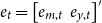 $e_t = \left [ e_{m,t} \,\, e_{y,t}\right ]^\prime$
denotes an
$e_t = \left [ e_{m,t} \,\, e_{y,t}\right ]^\prime$
denotes an $\left ( 1 + N_y\right ) \times 1$
vector of reduced form residuals, which follows a normal distribution. Zero coefficients on
$\left ( 1 + N_y\right ) \times 1$
vector of reduced form residuals, which follows a normal distribution. Zero coefficients on $m_{t-p}$
and
$m_{t-p}$
and $y_{t-p}$
indicate that the two shocks are independent of the lags of both
$y_{t-p}$
indicate that the two shocks are independent of the lags of both $m_t$
and
$m_t$
and $y_t$
.
$y_t$
. $y_t$
comprises real GDP, GDP deflator, the S&P 500 index, one-year Treasury bill yields, and EBP. Monthly interpolated values of GDP and GDP deflator (in log) are taken from Jarociński’s website. The S&P 500 index (in log) and the one-year Treasury yields are employed after taking monthly average. The EBP is sourced from Gilchrist and Zakrajšek (Reference Gilchrist and Zakrajšek2012). Besides the baseline variables, we additionally explore the responses of other low-frequency variables, including growth and inflation expectations, 10-year treasury yields, and term spreads between 10-year and 2-year treasury yields, by sequentially incorporating them into the model.
$y_t$
comprises real GDP, GDP deflator, the S&P 500 index, one-year Treasury bill yields, and EBP. Monthly interpolated values of GDP and GDP deflator (in log) are taken from Jarociński’s website. The S&P 500 index (in log) and the one-year Treasury yields are employed after taking monthly average. The EBP is sourced from Gilchrist and Zakrajšek (Reference Gilchrist and Zakrajšek2012). Besides the baseline variables, we additionally explore the responses of other low-frequency variables, including growth and inflation expectations, 10-year treasury yields, and term spreads between 10-year and 2-year treasury yields, by sequentially incorporating them into the model.
The sample period is from January 1990 to June 2019. The VAR includes 12 lags as in Jarociński and Karadi (Reference Jarociński and Karadi2020). In addition, given that sign restrictions only yield set identification because the decomposition of (4) is not unique (Baumeister and Hamilton, Reference Baumeister and Hamilton2015), we apply the median target rotation to obtain point estimates as in Fry and Pagan (Reference Fry and Pagan2011).Footnote 20
3. Comparison of the responses to the shocks
Moving on, this section presents the impulse responses which are estimated using alternatively identified CBI and MP shocks. We begin by displaying the responses to the benchmark shocks. Then, by comparing them with the results from candidate shocks, we discuss the nature of the identified shocks.
3.1 Responses from benchmark identification
Figure 1 illustrates the responses of the five baseline variables considered in Jarociński and Karadi (Reference Jarociński and Karadi2020) to the two distinct shocks (panel (a) for CBI shock and (b) for MP shock). In panel (a), the benchmark CBI shock leads to an increase in both output and the price level by about 9 and 3 basis points, respectively. It is also associated with a 155-basis-point increase in the S&P 500 index. The one-year Treasury bond yield rises by about 14 basis points. In addition, as the positive CBI shock delivers favorable news to financial conditions, the EBP falls by 7 basis points.
Responses from the benchmark identification. (a) CB information shock. (b) Monetary policy shock.
Notes: The figures present the impulse responses of the baseline variables to central bank information shocks (panel (a)) and monetary policy shocks (b), respectively, which are identified with the benchmark identification scheme. Each x- and y-axis represents the months after the occurrence of the shocks and the responses in percent or percentage points, respectively. The shaded areas are 90% confidence intervals.

Next, we can see the responses to a contractionary MP shock in panel (b). As the shock generates persistent effects, output and the price level drop by about 28 basis points and 11 basis points, respectively. The S&P 500 index declines by about 195 basis points. The one-year Treasury bond yield exhibits a 6-basis-point increase and its response is less persistent than that of other variables. Like the stock price, the EBP reflects tightened financial conditions, as it rises by about 11 basis points. Basically, the results above do not differ from those in Jarociński and Karadi (Reference Jarociński and Karadi2020).
In Figure 2, we report responses of four other variables—growth and inflation expectations, 10-year Treasury yield, and 10–2 year Treasury yield spread. As in Jarociński and Karadi (Reference Jarociński and Karadi2020), we estimate by adding them one by one to the baseline VAR model. The upper left figure in panel (a) shows that the growth expectation rises when a positive information shock hits. The impact on the inflation expectation exhibits similar responses, particularly in terms of direction, reaching a peak one year after the shock. The responses of the two expectations are conceptually consistent in that the information shock captures prospects for growth which is also positively correlated with inflationary pressure. The 10-year Treasury yield in the lower left panel shows an increase upon the same shock, implying that interest rates rise at the long end. However, when we see the response of the 10–2 year Treasury yield spread, the magnitude is larger on the short end as the spread declines at impact.
Responses of additional variables from benchmark identification. (a) CB information shock. (b) Monetary policy shock.
Notes: The figures present the impulse responses of additional variables, each added to the baseline, to central bank information shocks (panel (a)) and monetary policy shocks (b), respectively, which are identified with the benchmark identification scheme. Each x- and y-axis represents the months after the occurrence of the shocks and the responses in percent or percentage points, respectively. The shaded areas are 90% confidence intervals.

In panel (b), the upper left figure displays the response of the growth expectations to a contractionary monetary policy shock. As its negative effects materialize with a lag, the growth expectations exhibit a 10-basis-point fall one year after the shock. Responses of the inflation expectations show a similar pattern with an 8-basis-point decline at the nadir. The 10-year Treasury bond yield increases initially at impact, but the response becomes statistically significant in approximately two years.Footnote 21 Similar to the positive information shock, the contractionary monetary policy shock lowers the 10–2 year Treasury yield spread.
Taking the above results as a benchmark, in what follows, we sequentially present and compare the impulse responses to the candidate CBI and MP shocks. The candidate shocks are decomposed from monetary policy surprises using alternative instruments from four categories based on (i) New Keynesian, (ii) Fama–French factor, (iii) risk appetite, and (iv) commodity and currency.
3.2 Responses from the New Keynesian-based identification
First of all, we present responses to the shocks identified using r-star and inflation expectations, which are cornerstones shaping the effects of monetary policy in the New Keynesian framework.
3.2.1 Identification with r-stars
First, we investigate the responses to the shocks identified with five r-star measures.Footnote 22 For convenience, we refer to the candidate CBI shock and the candidate monetary policy shock as “r-star CBI shock” and “r-star MP shock,” respectively.
Responses from the identification with r-star. (a) CB information shock. (b) Monetary policy shock.
Notes: The figures present the impulse responses of the baseline variables to central bank information shocks (panel (a)) and monetary policy shocks (b), respectively, which are identified with r-star. Each x- and y-axis represents the months after the occurrence of the shocks and the responses in percent or percentage points, respectively. The shaded areas are 90% confidence intervals.

As before, panel (a) of Figure 3 displays the responses to a positive r-star CBI shock. Both output and the price level increase, resembling movements driven by Jarociński and Karadi’s (Reference Jarociński and Karadi2020) CBI shock. Compared with the responses from the benchmark identification, it is conspicuous that the responses of GDP and GDP deflator are much larger—almost four times greater. In light of the overall pattern, the S&P 500 index appears to show a more telling difference from the benchmark than other variables. While the benchmark information shock generates a substantial impact immediately, the r-star CBI shock barely changes the stock price at impact. This aspect would not be an appealing feature for a candidate CBI shock in that, although a positive response of real output persists, the forward-looking variable, the S&P 500 index, stays almost still at impact. The responses of the one-year Treasury yield and the EBP show similar patterns to the benchmark, albeit with greater magnitudes.
We now look into responses to a contractionary r-star MP shock (panel (b)). Both GDP and GDP deflator decline as in the benchmark. However, the significance of the response in GDP deflator is limited, with wide confidence intervals. The stock price index shows lagged responses. The S&P 500 index rises slightly at impact, but subsequently falls by 1%, taking more than six months to exhibit a significant decline. Along with the lagged response of the S&P 500 index, this result would undermine the grounds for it being a valid candidate for a monetary policy shock, compared to the benchmark.
Responses of additional variables from the identification with r-star. (a) CB information shock. (b) Monetary policy shock.
Notes: The figures present the impulse responses of additional variables, each added to the baseline one by one, to central bank information shocks (panel (a)) and monetary policy shocks (b), respectively, which are identified with r-star. Each x- and y-axis represents the months after the occurrence of the shocks and the responses in percent or percentage points, respectively. The shaded areas are 90% confidence intervals.

Figure 4 presents the responses of growth and inflation expectations, 10-year Treasury yield, and 10–2 year Treasury yield spread. In terms of general tendency, many of the results look similar to the responses to Jarociński and Karadi’s (Reference Jarociński and Karadi2020) CBI and MP shocks. However, specific dynamics are slightly different between the r-star CBI and the baseline CBI shocks. In panel (a) which displays responses to an r-star CBI shock, growth expectations become more positive upon the occurrence of the shock. The rise in the expectation gradually fades akin to the benchmark but the trajectory of impulse response is more or less bumpy in this case. Inflation expectations also rise with a stronger initial response than in the benchmark. While the 10-year Treasury yield peaks in six months in the benchmark, it takes about two years with a bimodal shape and smaller magnitudes in this case. The declines in the 10–2 year Treasury yield spread after the r-star CBI shock are more persistent than those observed after the benchmark CBI shock.
Responses to the r-star MP shock more closely resemble the benchmark MP shock, compared with the above. The negative turn of growth and inflation expectations is pronounced in about one year as in the benchmark responses. The overall rising pattern in the 10-year Treasury yield is similar. The 10–2 year Treasury yield spread declines immediately and remains lower for one year approximately after both of the benchmark and the r-star MP shock.
3.2.2 Identification with inflation expectations
As discussed in Section 2, CBI and MP shocks can co-vary with inflation expectations in opposite directions. We distinguish between the two shocks depending on the sign of changes in inflation expectation, labeling them as “EINF CBI shock” and “EINF MP shock.” For this identification, we employ two measures of inflation expectations provided separately by Consensus Economics and the Cleveland Fed.Footnote 23
Responses from the identification with inflation expectations (Consensus Economics). (a) CB information shock. (b) Monetary policy shock.
Notes: The figures present the impulse responses of the baseline variables to central bank information shocks (panel (a)) and monetary policy shocks (b), respectively, which are identified with Consensus Economics’ inflation expectation. Each x- and y-axis represents the months after the occurrence of the shocks and the responses in percent or percentage points, respectively. The shaded areas are 90% confidence intervals.

Figure 5 presents the impulse responses to shocks identified with Consensus Economics’ inflation expectations data. The shock does not generate responses aligning well with those by standard CBI shock. As shown in panel (a), GDP and the S&P 500 index fall when a positive EINF CBI shock hits, although the GDP deflator rises briefly. In addition, the EBP rises after the shock.
The responses to a contractionary EINF MP shock in panel (b) appear roughly consistent with theoretical priors. GDP and GDP deflator declines, while the EBP rises. However, their responses soon become statistically insignificant. Thus, the EINF MP shock does not produce very convincing outcomes.
3.3 Responses from the Fama–French factors-based identification
Next, the responses of variables to the alternative CBI and MP shocks, identified via Fama–French’s HML and SMB factors, are presented.
3.3.1 Identification with HML factor
We first examine impulse responses to identified shocks with HML. The candidate shocks are denoted as the “HML CBI shock” and “HML MP shock,” respectively. Panel (a) of Figure 6 shows that the HML CBI shock leads to an increase in both output and the price level. The shock also raises the S&P 500 index without a lag, unlike the r-star CBI shock which fails to generate the immediate response. The one-year Treasury bond yield rises with a hump shape as in the benchmark case. In addition, as the EBP falls at impact and rebounds afterward, it changes with a similar pattern to the impulse responses of the Jarociński and Karadi’s (Reference Jarociński and Karadi2020) CBI shock.
Responses from the identification with HML. (a) CB information shock. (b) Monetary policy shock.
Notes: The figures present the impulse responses of the baseline variables to central bank information shocks (panel (a)) and monetary policy shocks (b), respectively, which are identified with HML factor. Each x- and y-axis represents the months after the occurrence of the shocks and the responses in percent or percentage points, respectively. The shaded areas are 90% confidence intervals.

In panel (b), GDP decreases responding to the HML MP shock, and its decline is more visible several months after the initial impact as in the benchmark. Similarly, GDP deflator falls, exhibiting movements typical of a monetary policy shock. The HML MP shock is also successful in generating an immediate response in the S&P 500 index. The one-year Treasury bond yield rises right after the shock and the increase soon becomes insignificant. These movements are also observed in the responses to the benchmark MP shock. The HML MP shock drives up the EBP, implying its tightening effects on financial conditions.
Responses of additional variables from the identification with HML. (a) CB information shock. (b) Monetary policy shock.
Notes: The figures present the impulse responses of additional variables, each added to the baseline one by one, to central bank information shocks (panel (a)) and monetary policy shocks (b), respectively, which are identified with HML factor. Each x- and y-axis represents the months after the occurrence of the shocks and the responses in percent or percentage points, respectively. The shaded areas are 90% confidence intervals.

So far, the responses of the five variables to HML CBI and MP shocks are in line with those to benchmark CBI and MP shocks. In addition, compared with other candidates so far, HML CBI and MP shocks yield responses closest to those with the benchmark identification. In particular, whereas r-star CBI and MP shocks fail, HML CBI and MP shocks succeed in replicating the initial rise and fall in the S&P 500 index. We examine if additional variables exhibit similarities in responses with Figure 7. Panel (a) shows that the HML CBI shock improves the growth expectation as in the benchmark. It also raises the inflation expectations with more front-loaded effects than benchmark CBI shock. The 10-year Treasury yield increases and peaks six months after the shock, whose timing is identical to that in the benchmark. The 10–2 year Treasury yield spread shows similar declines responding to the HML CBI and benchmark CBI shocks, as the short-end rate rises higher.
In response to the HML MP shock, outlooks for growth and inflation decline in line with intuition. Compared with benchmark MP shock, the HML MP shock generates more rapid responses. Significant declines in growth and inflation follow in one and three months, respectively, after the HML MP shock, while taking about a year after benchmark shock. The 10-year Treasury yield shows an increase but, as 2-year yield rises more sharply, the 10–2 year yield spread decreases. The overall patterns of the two IRFs to the HML MP shock are not much different from those of the benchmark impulse responses.
Based on the results, HML CBI and MP shocks share common features with the standard CBI and MP shocks. They generate responses of output, prices, and their expectations, predicted by conventional wisdom. Besides, responses of financial variables to HML CBI and MP shocks are similar to those to Jarociński and Karadi’s (Reference Jarociński and Karadi2020) CBI and MP shocks. These results suggest that daily HML data can be a useful alternative to the high-frequency S&P 500 data to identify CBI and MP shocks.Footnote 24
3.3.2 Identification with SMB factor
We also investigate shocks identified with changes in SMB factor, that is, the return spreads between small- and large-cap stocks. Assuming that small firms benefit from better economic outlooks and looser financial conditions more than large firms, we identify a shock raising (lowering) SMB as a candidate CBI (MP) shock, referring to them as “SMB CBI (MP) shock.”
Responses from the identification with SMB. (a) CB information shock. (b) Monetary policy shock.
Notes: The figures present the impulse responses of additional variables, each added to the baseline one by one, to central bank information shocks (panel (a)) and monetary policy shocks (b), respectively, which are identified with SMB factor. Each x- and y-axis represents the months after the occurrence of the shocks and the responses in percent or percentage points, respectively. The shaded areas are 90% confidence intervals.

In panel (a) of Figure 8, GDP responds positively to an SMB CBI shock. The shock has a positive impact on output for the first several months. The responses of the GDP deflator are not consistent with the conventional prior for a CB information shock, as it falls rather than rises. The S&P 500 index increases with two humps, while its initial response is almost nil. The one-year Treasury yield shows acceptable responses, but the EBP does not as it increases at impact.
Compared with the responses to an SMB CBI shock, those of GDP to an SMB MP shock are less clear.Footnote 25 GDP appears to respond negatively in panel (b), yet the declines are not significant. The responses of the GDP deflator are the opposite of those to a standard MP shock, as it rises after an SMB MP shock. Like the response to an SMB CBI shock, the stock price index does not respond immediately although it tends to fall. The initial unresponsiveness is observed in the EBP. It rises in about six months after the SMB MP shock.
3.4 Responses from the risk appetite-based identification
Among various proxies for risk appetite measures, four indicators are selected for the decomposition of monetary policy surprises. They are risk aversion, VIX, EBP, and credit spread, all broadly used in related empirical studies. (Details of results using the last two instruments are reported in Online Appendix B.) The findings reveal nuanced differences in the responses created by each shock, indicating distinct information among them.
3.4.1 Identification with risk aversion
We consider a shock lowering (raising) risk aversion as a candidate CBI (MP) shock, labeling them as “risk aversion CBI (MP) shock.” In the identification, we use the daily risk aversion index by Bekaert et al. (Reference Bekaert, Engstrom and Xu2021) (BEX index) as a risk aversion measure.
The impulse responses to the identified shocks are presented in Figure 9. Panel (a) displays responses to a risk aversion CBI shock. When the information shock increases risk appetite, both output and the price level rise. That said, the S&P 500 index does not show a significant increase, differing from the response to the benchmark CBI shock. The responses of the one-year Treasury yield and the EBP are in line with the benchmark.
All responses to the risk aversion MP shock are similar to standard ones. Specifically, both GDP and the GDP deflator decline. In addition, the stock price index exhibits a significant fall. The one-year Treasury yield rises, and the EBP increases at impact, suggesting a straightforward effect of higher risk aversion.
Responses from the identification with risk aversion. (a) CB information shock. (b) Monetary policy shock.
Notes: The figures present the impulse responses of the baseline variables to central bank information shocks (panel (a)) and monetary policy shocks (b), respectively, which are identified with risk aversion index (Bekaert et al. Reference Bekaert, Engstrom and Xu2021). Each x- and y-axis represents the months after the occurrence of the shocks and the responses in percent or percentage points, respectively. The shaded areas are 90% confidence intervals.

The identification with risk aversion generates similar responses to Jarociński and Karadi’s (Reference Jarociński and Karadi2020) identification in many aspects. In particular, responses of output and the price level to the risk aversion CBI and MP shocks are consistent with standard patterns.Footnote 26 In addition, all other variables, except the S&P 500 index, demonstrate acceptable responses to both types of shocks.
Responses of additional variables from the identification with risk aversion. (a) CB information shock. (b) Monetary policy shock.
Notes: The figures present the impulse responses of additional variables, each added to the baseline one by one, to central bank information shocks (panel (a)) and monetary policy shocks (b), respectively, which are identified with risk aversion index (Bekaert et al. Reference Bekaert, Engstrom and Xu2021). Each x- and y-axis represents the months after the occurrence of the shocks and the responses in percent or percentage points, respectively. The shaded areas are 90% confidence intervals.

Considering this, one may view the unresponsiveness of S&P 500 as the only problem to be solved. However, we find more issues. Panels (a) and (b) in Figure 10 show responses of inflation and growth expectations, 10-year Treasury yield, and 10–2 year Treasury yield spread to each shock. While expectation variables move in line with standard responses, the 10-year Treasury yield in panel (a) presents a noticeable difference. It initially falls when the risk aversion CBI shock hits. Besides, the initial response of yield spread to a risk aversion MP shock is contrary to that to a benchmark MP shock. As the 10-year yield rises more sharply, the spread widens at impact, whereas it narrows when benchmark MP shock hits. In sum, the identification with risk aversion generates standard responses of macroeconomic variables. However, given that results for financial variables are not entirely successful, it does not appear to be a good alternative to the benchmark identification.
3.4.2 Identification with VIX
In addition, we examine the results from an identification using the VIX, the stock market option-based implied volatility. The motivation for this analysis is related to the identification with risk aversion. Bekaert et al. (Reference Bekaert, Hoerova and Duca2013) decompose the VIX into risk aversion and uncertainty components and find that a loose monetary policy decreases both of them, having a larger effect on risk aversion. Thus, identification with the VIX captures changes in risk aversion in part. We identify a shock lowering (raising) the VIX as a candidate CBI (MP) shock, labeling them as “VIX CBI (MP) shock,” postulating that a rise in the high-frequency measure has opposite effects on the daily VIX depending on the type of shock.
Responses from the identification with VIX. (a) CB information shock. (b) Monetary policy shock.
Notes: The figures present the impulse responses of the baseline variables to central bank information shocks (panel (a)) and monetary policy shocks (b), respectively, which are identified with the VIX index. Each x- and y-axis represents the months after the occurrence of the shocks and the responses in percent or percentage points, respectively. The shaded areas are 90% confidence intervals.

The responses suggest that this identification is not promising as an alternative. First of all, in Panel (a) of Figure 11, we see key macroeconomic variables fall after a VIX CBI shock. In addition, the S&P 500 index slightly rises at impact but afterward falls by 2 percent. The adverse effect is also observed in the EBP as it increases immediately. Thus, a VIX CBI shock is not thought to deliver favorable news to the real economy or the financial market. Some responses to a VIX MP shock also undermine its candidacy. While the shock tends to drive down GDP, it does not have significant effects on the GDP deflator. In addition, rises in the stock price, instead of falls, are pronounced although they are not significant.
3.5 Responses from the commodity- and currency-based identification
Commodity and currency markets are recognized for their informational merits such as price efficiency, forward-looking information, and information processing ability (Bohl et al. Reference Bohl, Irwin, Pütz and Sulewski2023; Chan et al. Reference Chan, Tse and Williams2011). Taking into account the nature of these markets, we assess the informational content of the candidate MP and CBI shocks sorted out by oil prices and exchange rates, respectively.
3.5.1 Identification with oil price
We first examine the results which exploit oil prices as a candidate for identification. Oil prices tend to reflect not only the demand at hand but also future demand prospects. Thus, we identify candidate information shocks (“oil CBI shock”) and monetary policy shocks (“oil MP shock”) with daily WTI oil prices. A natural conjecture would be that oil prices rise if there is positive news or a stimulus for the economy, vice versa. In fact, Yang et al. (Reference Yang, Zhang and Chen2023) empirically document that a contractionary MP shock lowers crude oil prices while a positive CBI shock raises them. Thus, we identify a candidate CBI (MP) shock if the oil price rises (falls).
Responses from the identification with oil price. (a) CB information shock. (b) Monetary policy shock.
Notes: The figures present the impulse responses of the baseline variables to central bank information shocks (panel (a)) and monetary policy shocks (b), respectively, which are identified with the WTI crude oil prices. Each x- and y-axis represents the months after the occurrence of the shocks and the responses in percent or percentage points, respectively. The shaded areas are 90% confidence intervals.

Panel (a) in Figure 12 presents responses to the oil CBI shock. Impulse responses on the right-hand side indicate that this does not produce consistent results with the benchmark identification. Although GDP shows a tiny increase initially, its decline becomes more visible within a year. In addition, the S&P 500 index and the EBP move in opposite directions to those responding to benchmark CBI shock at impact. Other variables, the GDP deflator and the one-year Treasury yield, exhibit similar responses to the benchmark results.
Responses to the oil MP shock in panel (b) also fail to reproduce required features. GDP falls slightly at impact but turns to a rise although the magnitude is not large. The S&P 500 index initially shows a small increase, not a decrease, which becomes insignificant. The EBP declines, in contrast to typical tightening effects of monetary policy. As before, responses of the GDP deflator and the Treasury yield look more reasonable than those of other variables.
3.5.2 Identification with exchange rates
In Jarociński (Reference Jarociński2022), CBI and MP shocks generate opposite responses of exchange rates.Footnote 27 We identify candidate CBI (MP) shock if the US dollar index falls (rises), based on the results in Jarociński (Reference Jarociński2022). Jarociński (Reference Jarociński2022) considers responses of exchange rates of euro against US dollar and broad dollar index excluding euro against US dollar, separately. We employ the consolidated US dollar index for identification. Since the direction of initial responses is identical in Jarociński (Reference Jarociński2022), using the US dollar index could be a valid approach. We refer to two candidate shocks as “EXR CBI shock” and “EXR MP shock.”
Responses from the identification with US dollar index. (a) CB information shock. (b) Monetary policy shock.
Notes: The figures present the impulse responses of the baseline variables to central bank information shocks (panel (a)) and monetary policy shocks (b), respectively, which are identified with the US dollar index. Each x- and y-axis represents the months after the occurrence of the shocks and the responses in percent or percentage points, respectively. The shaded areas are 90% confidence intervals.

In Figure 13, panel (a) displays responses to an EXR CBI shock. Unlike the reactions to the benchmark CBI shock, GDP eventually declines after a small and short-lived increase, and GDP deflator falls at impact and does not rise above zero afterwards. The stock price index does not show significant responses in either direction. Although the one-year Treasury yield rises, the EBP tends to rise in contrast to the benchmark result.
Impulse responses to an EXR MP shock look like those to a standard monetary policy shock. GDP and the GDP deflator declines after a contractionary EXR MP shock. The S&P 500 index also falls. Although its size is small, the one-year Treasury yield shows an increase at impact. The response of the EBP to this shock resembles that to benchmark MP shock.
Broadly, the exchange rate-based identification shows the same failure as the expected inflation-based identification (see Figure A1). Neither of them generate anticipated results from a standard CBI shock, with each variable moving in the same direction, except for the S&P 500 index. Identifications with exchange rates for individual currencies such as US dollar against JPY or British pound (GBP) do not resolve the problem.Footnote 28 Respective EXR CBI shocks drive down the GDP deflator and the stock price and drive up the EBP. In comparison, MP EXR shocks identified with JPY or GBP generate impulse responses consistent with standard ones. Thus, exchange rate-based identifications have limitations in isolating information shocks.
3.6 Robustness checks
Online Appendix E reports additional results from a battery of robustness checks. The distinct responses to the two shocks, in particular those identified with HML factors, are greatly robust to (i) the samples of pre-zero lower bound period, (ii) the short-run zero restrictions on GDP and the GDP deflator, (iii) the shocks identified with a median value approach, and (iv) 3-month VAR lag, chosen based on the information criteria.Footnote 29
4. Informational content in the shocks
What accounts for the differences in responses of variables between the benchmark and the candidates? Conceptually, the deviations reflect the different informational content in each shock. To evaluate the information embodied in the candidate shocks, we adopt a simple yet straightforward strategy, taking into account the methods which are commonly used in IV approach.Footnote 30 Specifically, we assess the identified shocks from the perspectives of (i) relevance and (ii) exogeneity. More precisely, we examine the cross-correlations of each candidate shock with the benchmark shocks and with other monetary policy-related or structural shocks.
4.1 Snapshots: Benchmark shocks and candidate shocks
To have a bird’s eye view of each shock identified via an alternative instrument, we first present benchmark CBI and MP shocks (panel (a) in Figure 14) and the corresponding HML-based shocks (panel (b)) the identified shocks, which produced quite similar impulse responses to the benchmarks, for comparison. The figure highlights that the benchmark and candidate shocks share a substantial, but not entire, amount of common information.
Benchmark and HML-based shocks. (a) Benchmark shocks. (b) HML-based shocks.
Notes: The figure displays the correlations of candidate central bank information shocks (panel (a)) and monetary policy shocks (b), respectively, in a heat map format. The shocks are identified with the benchmark approach of Jarociński and Karadi (Reference Jarociński and Karadi2020) (BM) and the alternative methods.

Over the period, the fluctuations of both HML-based MP and CBI shocks largely resemble the benchmark, with some exceptions. In more detail, both shocks, identified either by BM or by HML, capture the episodes in 2001-02 and 2008-09 when the Fed responded vigorously to the adverse impacts of the dot-com crash and the global financial crisis. However, during the taper tantrum episode around 2013, there were strong negative HML CBI shocks and positive HML MP shocks, a pattern that was not observed in the benchmark shocks. Furthermore, in 2018, when the Fed began to slowly shrink its balance sheet, HML captures some significant positive MP shocks, whereas BM does not.Footnote 31
4.2 Correlations of the identified shocks
We now examine cross-correlations among the benchmark shocks and the other candidate shocks. By doing so, we can assess the extent to which each identified shock shares common information with benchmark shock and with others. It can also serve as an evaluation of the validity for alternative identification, which was presented in Section 3.
Cross-correlations. As a first pass, the correlations for CBI shocks (panel (a)) and MP shocks (panel (b)) are summarized in a heat map format in Figure 15.
Correlations of candidate shocks. (a) Candidate CBI shocks. (b) Candidate MP shocks.
Notes: The figure displays the correlations of candidate central bank information shocks (panel (a)) and monetary policy shocks (b), respectively, in a heat map format. The shocks are identified using the benchmark approach of Jarociński and Karadi (Reference Jarociński and Karadi2020) (BM) and the alternative methods. EINF(C.E.) and EINF(C.F.) denote inflation expectations of the Consensus Economics and the Cleveland Fed, respectively. RAVER, EBP, and CSP represent risk aversion index, excess bond premium, and credit spreads. In addition, USDIDX, JPY, and GBP represent US dollar index, US dollar against Japanese yen, and British pound.

The first row in panel (a) presents the correlations with benchmark (BM) CBI shocks. Overall, they are significant, albeit not very high, as the average correlation of each identified shock with BM is 0.38. Among them, shocks identified with HML exhibit the highest correlation (0.57) with BM. Those with risk aversion indices by Bekaert et al. (Reference Bekaert, Hoerova and Duca2013) show the second-highest correlation (0.55). The consensus inflation expectations (EINF(C.E.)) CBI shocks and EBP CBI shocks have correlations of 0.52 and 0.51, respectively, which are not substantially different from the highest one. Somewhat surprisingly, r-star CBI shocks have a low correlation of 0.25. In addition, they have low correlations (average not exceeding 0.20) with the rest of the shocks. Thus, r-star CBI shocks seem to contain quite distinct information from other candidates. SMB and EXR (USDIDX) CBI shocks also yield low correlations, 0.21 and 0.25, respectively, with the BM shocks. However, their average correlations with other shocks are 0.45 and 0.36, respectively, much higher than that of shocks identified using r-star. Given that the correlations between BM shocks and most of the identified shocks are, by and large, not very high, common information would not be the main reason if the impulse responses to them were similar to those to benchmark CBI shock.
Next, panel (b) of Figure 15 displays correlations between benchmark and candidate MP shocks. The average correlation of each identified shock with BM is quite high, recorded at around 0.61. It is notable that r-star MP shocks show the highest correlation (0.86) with BM, contrasting with the low correlation of its CBI counterpart (i.e., r-star CBI shocks) with BM CBI shocks. The second-highest correlation with BM (0.79) is observed in HML MP shocks. Like the HML-based identification for CBI shocks, that for MP shocks produces candidate shocks which are highly correlated with BM. Identification based on the EBP also yields highly correlated shock series, with the third-highest correlation of 0.72. Among the rest of the candidates, inflation expectations (EINF), and risk aversion (RAVER) show relatively high correlations of around 0.7.Footnote 32
Overall, candidate CBI and MP shocks identified with HML display the closest co-movements with both types of Jarociński and Karadi’s (Reference Jarociński and Karadi2020) shocks. Nonetheless, since this feature would not be enough to guarantee similarities in impulse responses between the two identifications, the results from HML-based identification are remarkable. That is, the imperfect correlation between HML CBI shocks and BM CBI shocks (0.57) suggests that each CBI shock has enough room to contain distinct information. For this reason, provided that the benchmark identification is the best approach to isolate central bank information, it would be challenging to obtain the stylized impulse responses with the alternative identification.
Exogeneity test. Another way of examining the correlations among the benchmark and the identified shocks is to implement an exogeneity test. This is done by estimating a battery of univariate regressions, given as:
 \begin{align} \varepsilon ^{j}_{BM,t} = \beta _0 + \beta _{i} \varepsilon ^{j}_{i,t} + \theta _{i,t} \end{align}
where $\varepsilon ^{j}_{BM,t}$
denotes the benchmark shocks of
$\varepsilon ^{j}_{BM,t}$
denotes the benchmark shocks of $j \in \{CBI, MP\}$
, while
$j \in \{CBI, MP\}$
, while $\varepsilon ^{j}_{i,t}$
corresponds to the alternatively identified
$\varepsilon ^{j}_{i,t}$
corresponds to the alternatively identified $i$
-th shocks other than the benchmark. Hence, testing the null hypothesis
$i$
-th shocks other than the benchmark. Hence, testing the null hypothesis $\beta _{i}=0$
is equivalent to determining whether the benchmark shocks are correlated with the alternative shocks.
$\beta _{i}=0$
is equivalent to determining whether the benchmark shocks are correlated with the alternative shocks.
Table 2 summarizes the results, with columns (a) and (b) reporting for CBI and MP shocks, respectively. To a large extent, the estimation results reaffirm the findings from Figure 15. Correlations between the benchmark and the alternative shocks are significant, with only one exception (US dollar index-based MP shocks).
Correlation test results

Notes: This table presents the estimates of regression (6) ( $\beta _{i,t}^{j}$
for
$\beta _{i,t}^{j}$
for $j\in \{CBI, MP\}$
), each coming from a separate regression on an alternative instrument. SE denotes Newey–West heteroskedasticity and auto-correlation consistent standard error. Acronyms in the first column are identical to those in Figure 15.
$j\in \{CBI, MP\}$
), each coming from a separate regression on an alternative instrument. SE denotes Newey–West heteroskedasticity and auto-correlation consistent standard error. Acronyms in the first column are identical to those in Figure 15.
4.3 The relations of the identified shocks with other structural shocks
With our focus kept on the information in the candidate shocks, we now explore their correlations with other structural shocks. In doing so, we estimate a set of regressions (7), which is similar to equation (6) but assigns the candidate shocks and the other shocks to the dependent and independent variables, respectively.
 \begin{align} \epsilon ^c_{j,t} = \beta _0 + \beta _i \epsilon _{i,t} + \zeta _{i,t} \end{align}
where $\epsilon ^c_{j,t}$
denotes the 13 candidates for the
$\epsilon ^c_{j,t}$
denotes the 13 candidates for the $j$
shock
$j$
shock $(j\in \{CBI, MP\})$
.
$(j\in \{CBI, MP\})$
. $\epsilon _{i,t}$
represents other monetary policy-related or structural shocks. The statistical significance of the estimates
$\epsilon _{i,t}$
represents other monetary policy-related or structural shocks. The statistical significance of the estimates $\hat {\beta }_i$
is mutually compared to evaluate the informational content in terms of
$\hat {\beta }_i$
is mutually compared to evaluate the informational content in terms of $\epsilon _{i,t}$
.
$\epsilon _{i,t}$
.
For $\epsilon _{i,t}$
, we first employ various monetary policy-related shocks to assess whether the candidate shocks successfully capture the information associated with monetary policy shocks and, if so, to what extent. Specifically, three types of monetary policy-related shocks are used, taken from Bu et al. (Reference Bu, Rogers and Wu2021) (BRW), Cieslak and Schrimpf (Reference Cieslak and Schrimpf2019) (CS
$\epsilon _{i,t}$
, we first employ various monetary policy-related shocks to assess whether the candidate shocks successfully capture the information associated with monetary policy shocks and, if so, to what extent. Specifically, three types of monetary policy-related shocks are used, taken from Bu et al. (Reference Bu, Rogers and Wu2021) (BRW), Cieslak and Schrimpf (Reference Cieslak and Schrimpf2019) (CS $^{\text{MP}}$
), and Romer and Romer (Reference Romer and Romer2000) (RR).
$^{\text{MP}}$
), and Romer and Romer (Reference Romer and Romer2000) (RR).
In addition, following Cieslak and Schrimpf (Reference Cieslak and Schrimpf2019) and Cieslak and Pang (Reference Cieslak and Pang2021), we consider financial shocks (CS $^{\text{F}}$
) and growth shocks (CS
$^{\text{F}}$
) and growth shocks (CS $^{\text{G}}$
), which are decomposed from monetary policy surprises. The two shocks are identified by exploiting the close relationship between MPS and market securities in an asset pricing framework. Along with the shocks, other types of financial and growth shocks are taken into account for comparison. Specifically, we implement correlation tests by including financial shocks by Gilchrist and Zakrajšek (Reference Gilchrist and Zakrajšek2012) (GZ) and VAR-based news or productivity shocks by Barsky and Sims (Reference Barsky and Sims2012) (VAR(3)), and Beaudry and Portier (Reference Beaudry and Portier2004) (VAR(4)).
$^{\text{G}}$
), which are decomposed from monetary policy surprises. The two shocks are identified by exploiting the close relationship between MPS and market securities in an asset pricing framework. Along with the shocks, other types of financial and growth shocks are taken into account for comparison. Specifically, we implement correlation tests by including financial shocks by Gilchrist and Zakrajšek (Reference Gilchrist and Zakrajšek2012) (GZ) and VAR-based news or productivity shocks by Barsky and Sims (Reference Barsky and Sims2012) (VAR(3)), and Beaudry and Portier (Reference Beaudry and Portier2004) (VAR(4)).
Relatedly, oil-related shocks, including oil price shocks (Kilian, Reference Kilian2008: Oil $^{\text{P}}$
) and oil production shocks (Ha et al. Reference Ha, Kose and Ohnsorge2019: Oil
$^{\text{P}}$
) and oil production shocks (Ha et al. Reference Ha, Kose and Ohnsorge2019: Oil $^{\text{Q}}$
), are also compared with the candidate shocks. Basically, oil-related shocks have been interpreted as cost-push shocks, that is, exogenous shifts in the aggregate supply curve, generating substantial impacts. Since their occurrence is not rare, it is worth suspecting the relevance of candidates with the oil-related shocks.Footnote
33
$^{\text{Q}}$
), are also compared with the candidate shocks. Basically, oil-related shocks have been interpreted as cost-push shocks, that is, exogenous shifts in the aggregate supply curve, generating substantial impacts. Since their occurrence is not rare, it is worth suspecting the relevance of candidates with the oil-related shocks.Footnote
33
Last, we also compare the candidate shocks with uncertainty indicators related to monetary policy— economic policy uncertainty by Baker et al. (Reference Baker, Bloom and Davis2016) (EPU) and monetary policy uncertainty by Husted et al. (Reference Husted, Rogers and Sun2020) (MPU).Footnote 34 Recent literature corroborates the importance of uncertainty associated with monetary policy and its close relationship with monetary policy surprises (De Pooter et al. Reference De Pooter, Favara, Modugno and Wu2021; Tillmann, Reference Tillmann2020; Swanson, Reference Swanson2006).Footnote 35
The estimation results of equation (7) are summarized in Figures 16–A34 of Online Appendix F. Panels (a) and (b) in each figure summarize the estimation results for CBI shocks and MP shocks, respectively. Each bar represents the 90% confidence intervals of the estimate of $\beta _i$
in equation (7). In addition, the tips of the bars are colored dark for estimates with statistical significance, and left blank for those with insignificance.
$\beta _i$
in equation (7). In addition, the tips of the bars are colored dark for estimates with statistical significance, and left blank for those with insignificance.
4.3.1 Benchmark shocks
Figure 16 first presents the significance of estimates from the regression of benchmark shocks on the aforementioned structural shocks. To a large extent, the benchmark CBI and MP shocks are exogenous to the other types of structural shocks with only a few exceptions. For MP shocks, the benchmark CBI shocks have positive correlations with BRW and RR shocks. This result suggests that the two monetary policy-related shocks may contain some information associated with the Fed’s assessment of economic prospects.Footnote
36
Interestingly, on the other hand, the benchmark MP shocks are positively correlated only with BRW. The results conjointly suggest that the shocks identified following Jarociński and Karadi (Reference Jarociński and Karadi2020) may possess informational content, distinguished to some degree from the monetary shocks identified using other approaches. For other types of structural shocks, statistically significant correlations are not observed with an exception for CS $^{\text{G}}$
shocks, indicating that the identified benchmark shocks are highly exogenous.
$^{\text{G}}$
shocks, indicating that the identified benchmark shocks are highly exogenous.
Confidence intervals for the estimates from equation (7): benchmark. (a) CB information shock. (b) Monetary policy shock.
Notes: The figures summarize the confidence intervals of the estimates ( $\hat {\beta }_i$
) from the regression (7) where the shocks identified with r-stars are employed as dependent variables. Panels (a) and (b) report the results for central bank information shocks and monetary policy shocks, respectively. In each panel, the left-hand side chart presents the results for MP-related shocks (CS
$\hat {\beta }_i$
) from the regression (7) where the shocks identified with r-stars are employed as dependent variables. Panels (a) and (b) report the results for central bank information shocks and monetary policy shocks, respectively. In each panel, the left-hand side chart presents the results for MP-related shocks (CS $^{\text{MP}}$
: Cieslak and Schrimpf (Reference Cieslak and Schrimpf2019), BRW: Bu et al. (Reference Bu, Rogers and Wu2021), RR: Romer and Romer (Reference Romer and Romer2000)), while the right-hand side chart shows those for other structural shocks ((i) financial shocks – CS
$^{\text{MP}}$
: Cieslak and Schrimpf (Reference Cieslak and Schrimpf2019), BRW: Bu et al. (Reference Bu, Rogers and Wu2021), RR: Romer and Romer (Reference Romer and Romer2000)), while the right-hand side chart shows those for other structural shocks ((i) financial shocks – CS $^{\text{RP}}$
: Cieslak and Schrimpf (Reference Cieslak and Schrimpf2019), GZ: Gilchrist and Zakrajšek (Reference Gilchrist and Zakrajšek2012), (ii) growth shocks – CS
$^{\text{RP}}$
: Cieslak and Schrimpf (Reference Cieslak and Schrimpf2019), GZ: Gilchrist and Zakrajšek (Reference Gilchrist and Zakrajšek2012), (ii) growth shocks – CS $^{\text{G}}$
: Cieslak and Schrimpf (Reference Cieslak and Schrimpf2019), VAR(3): Barsky and Sims (Reference Barsky and Sims2012), VAR(4): Beaudry and Portier (Reference Beaudry and Portier2004), VAR(6): Levchenko and Pandalai-Nayar (Reference Levchenko and Pandalai-Nayar2020), (iii) oil shocks – Oil
$^{\text{G}}$
: Cieslak and Schrimpf (Reference Cieslak and Schrimpf2019), VAR(3): Barsky and Sims (Reference Barsky and Sims2012), VAR(4): Beaudry and Portier (Reference Beaudry and Portier2004), VAR(6): Levchenko and Pandalai-Nayar (Reference Levchenko and Pandalai-Nayar2020), (iii) oil shocks – Oil $^{\text{P}}$
: Kilian (Reference Kilian2008), Oil
$^{\text{P}}$
: Kilian (Reference Kilian2008), Oil $^{\text{Q}}$
: Ha et al. (Reference Ha, Kose and Ohnsorge2019), (iv) uncertainty – EPU: Baker et al. (Reference Baker, Bloom and Davis2016), MPU: Husted et al. (Reference Husted, Rogers and Sun2020)). The bars are 90% confidence intervals, with dark-colored tips indicating significant estimates and blank tips indicating non-significant estimates.
$^{\text{Q}}$
: Ha et al. (Reference Ha, Kose and Ohnsorge2019), (iv) uncertainty – EPU: Baker et al. (Reference Baker, Bloom and Davis2016), MPU: Husted et al. (Reference Husted, Rogers and Sun2020)). The bars are 90% confidence intervals, with dark-colored tips indicating significant estimates and blank tips indicating non-significant estimates.

4.3.2 New Keynesian-based shocks
We now compare the correlations between the candidate CBI and MP shocks which are identified with alternative instruments and the other types of structural shocks listed above. The shocks disentangled with New Keynesian-based instruments (r-stars and inflation expectations) are first examined. In Figure A23, the estimation results are presented for the shocks identified with r-star. R-star CBI shocks are negatively correlated with financial shocks (GZ), growth shocks (CS $^{\text{G}}$
), and uncertainty (EPU). More interestingly, they do not exhibit any correlations with other monetary policy-related shocks. Together with their low correlation with BM CBI shocks (0.25), these different natures of the r-star CBI shocks may contribute to the larger responses of macro variables compared to the benchmark. Meanwhile, r-star MP shocks are positively correlated only with oil price shocks, while they are positively correlated with BRW and RR monetary shocks. With their high correlation with BM MP shocks (0.86), the exogeneity of r-star MP shocks may result in the similarity of the response patterns to those of BM MP shocks, albeit short-lived.
$^{\text{G}}$
), and uncertainty (EPU). More interestingly, they do not exhibit any correlations with other monetary policy-related shocks. Together with their low correlation with BM CBI shocks (0.25), these different natures of the r-star CBI shocks may contribute to the larger responses of macro variables compared to the benchmark. Meanwhile, r-star MP shocks are positively correlated only with oil price shocks, while they are positively correlated with BRW and RR monetary shocks. With their high correlation with BM MP shocks (0.86), the exogeneity of r-star MP shocks may result in the similarity of the response patterns to those of BM MP shocks, albeit short-lived.
Figures A24 and A25 illustrate the confidence intervals of the estimates for the shocks identified with inflation expectation instruments, sourced from Consensus Economics and Cleveland Fed, respectively. Noticeably, EINF CBI and MP shocks are negatively correlated with various types of structural shocks, including growth and news shocks (for EINF(C.E.) CBI and MP), and uncertainty (for EINF(C.E.) CBI and EINF(C.F.) MP). On the whole, the large deviations from the benchmark responses at least partially reflect such differences in their informational content.
4.3.3 Fama–French factor-based shocks
The exogeneity test results for the shocks decomposed with Fama–French factor-based instruments are reported in Figures 17 (HML) and A26 (SMB), respectively. Looking into tests for HML-based shocks, the coefficients broadly resemble the pattern in tests for BM shocks. The significant relationship of the HML CBI shock with RR shocks is similar to that of BM CBI shocks. With most of the coefficients having the same signs, HML-based shocks provide a few significant cases only at the margin, such as coefficients on GZ and MPU. In addition, while the coefficient on EPU is significant for HML CBI shocks, it is marginally insignificant for BM CBI shocks.
Confidence intervals for the estimates from equation (7): HML. (a) CB information shock. (b) Monetary policy shock.
Notes: The figures summarize the confidence intervals of the estimates ( $\hat {\beta }_i$
) from the regression (7) where the shocks identified with Fama–French HML factor are employed as dependent variables. Panels (a) and (b) report the results for central bank information shocks and monetary policy shocks, respectively. In each panel, the left-hand side chart presents the results for MP-related shocks, while the right-hand side chart shows those for other structural shocks, including (i) financial shocks, (ii) growth shocks, (iii) oil shocks, and (iv) uncertainty. Acronyms on the x-axis correspond identically to those in Figure 16. The bars are 90% confidence intervals, with dark-colored tips indicating statistically significant estimates and blank tips indicating non-significant estimates.
$\hat {\beta }_i$
) from the regression (7) where the shocks identified with Fama–French HML factor are employed as dependent variables. Panels (a) and (b) report the results for central bank information shocks and monetary policy shocks, respectively. In each panel, the left-hand side chart presents the results for MP-related shocks, while the right-hand side chart shows those for other structural shocks, including (i) financial shocks, (ii) growth shocks, (iii) oil shocks, and (iv) uncertainty. Acronyms on the x-axis correspond identically to those in Figure 16. The bars are 90% confidence intervals, with dark-colored tips indicating statistically significant estimates and blank tips indicating non-significant estimates.

By contrast, for another Fama–French factor-based shocks, SMB shocks, the information goes against the grain with the benchmark shocks, despite being orthogonally identified. For example, the SMB-based identification yields a larger coefficient on BRW for CBI shocks than MP shocks, unlike the benchmark identification. This is likely due to their poor representation of monetary policy-related information.
4.3.4 Risk appetite-based shocks
Figures A27–A30 present the regression results to check the exogeneity of risk appetite-based shocks—RAVER, EBP, CSP, and VIX shocks. They show some contrasting patterns to BM shocks, having significant correlations with other types of structural shocks. For instance, RAVER CBI shocks have a larger coefficient on BRW for CBI shocks than MP shocks, containing characteristics of financial and news shocks to some extent, whereas BM CBI shocks do not. In the identification with EBP, both CBI and MP shocks display negative correlations with growth and news shocks. In addition, CSP and VIX CBI shocks appear negatively correlated with financial and growth shocks. The correlations of the two CBI shocks with growth shocks are at odds with the benchmark identification because growth shocks have a significant correlation with BM MP shocks, not BM CBI shocks. All things considered, these results suggest that the mixture of extraneous information and contrasting correlation patterns in risk appetite-based shocks contribute to the large deviations of the impulse responses from the benchmark results.Footnote 37
4.3.5 Commodity- and currency-based shocks
Finally, we provide the summaries of exogeneity test results for oil price-based shocks in Figure A31 and currency-based shocks in Figures A32–A34. Among them, WTI CBI shocks exhibit a problematic correlations with oil and growth shocks as well as correlation with uncertainty. Further, currency-based decomposed shocks, on the whole, appear to contain different content from the BM shocks. The shocks identified using USD index show insignificant correlations with other monetary policy shocks, being correlated with oil shocks. JPY-based MP shocks contain the information of EPU shocks, as do GBP-based MP shocks. GBP-based MP and CBI shocks are also significantly related to MPU and growth shocks, respectively. These features in currency-based identifications are inconsistent with the benchmark identification.
After all is said and done, the results jointly suggest that, although commodity- and currency-based shocks convey the information somewhat at odds with the benchmarks. The distinct nature of these candidate shocks may account for the large discrepancies in impulse responses between the benchmarks and the candidates, in particular for CBI shocks.
5. Conclusion
The recent pandemic crisis and the subsequent countermeasures implemented by central banks have refocused attention on the information in the policy decisions and communications. This paper examines the informational content embedded in the Fed’s policy announcements. To this end, we put together a range of candidate instruments aimed at disentangling monetary policy surprises into two components: pure MP and CBI shocks. The candidates are selected from various categories, including New Keynesian-based and Fama–French factor-based instruments. Then, we investigate the information conveyed by each decomposed shock, comparing the responses of economic variables with those to the benchmark MP and CBI shocks identified by Jarociński and Karadi (Reference Jarociński and Karadi2020).
Our findings shed light on the nature of each candidate shock in several aspects. First, the impulse responses to the two types of candidate shocks unveil the underlying information in each shock. From the comparisons of the impulse responses, we find that the HML factor effectively decomposes the monetary policy surprises. The reactions of economic variables to the shocks identified using HML align with theoretical predictions, almost comparable to the benchmark shocks. However, other candidate shocks could reproduce responses only partially consistent with stylized ones.
Second, the candidate shocks identified with alternative instruments exhibit positive correlations with the benchmark, albeit with noticeable differences. On average, candidate CBI shocks display positive yet relatively low correlations with the benchmark shock. On the other hand, candidate MP shocks show stronger positive correlations. Notably, for both types of shocks, shocks identified with the HML factor demonstrate superior correlations with the benchmark shock.
Furthermore, the exogeneity test results reveal that some candidates exhibit significant correlations with other macroeconomic shocks. Among them, HML-based shocks show the closest correlation pattern to the benchmark shocks. Combining with the aforementioned results, this suggests that other candidate shocks convey extraneous non-monetary policy-related information, distinct from the benchmark. This may, at least partly, account for the similarities or discrepancies between the responses to the benchmark and the candidate shocks. Notably, HML-based shocks show appealing properties as an alternative instrument for disentangling policy surprises.
Our findings and approach bear important implications for monetary policy studies. We demonstrate that the information encapsulated in the monetary policy surprises can also be effectively captured using different instruments, such as the HML factor, moving beyond the sole reliance on high-frequency stock price data. This underscores the need for further exploration into alternative sources for the shock decomposition. Of particular importance is the potential value of utilizing alternative instruments to facilitate identification in data-constrained environments and foster richer discussions on transmission mechanisms. In this vein, our approach can also be practical for emerging market economies, where central bank communication has become increasingly complex despite less developed financial markets. By applying our multi-pronged approach, researchers and policymakers in these economies can effectively disentangle the two distinct shocks using alternative instruments—for example, lower-frequency or non-financial data.
Supplementary material
The supplementary material for this article can be found at https://doi.org/10.1017/S1365100526101072.
Acknowledgments
The views expressed in this paper are solely the responsibility of the authors and should not be interpreted as reflecting the views of the Korea Capital Market Institute. The authors thank Sangyup Choi, Boreum Kwak, Julien Pinter (discussants), Jae Won Lee, Jin Il Kim, Noh-Sun Kwark, Youngjin Yun, Robert Czudaj, Joscha Beckmann, and participants at the Bank of Korea seminar, Korean Society for Macroeconomic Dynamics seminar, and the 4th Workshop on Financial Econometrics and Empirical Modeling of Financial Markets.


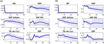
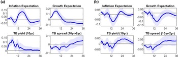
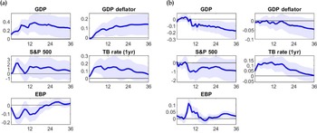
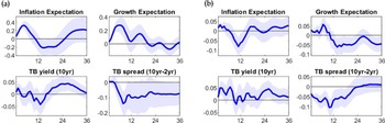
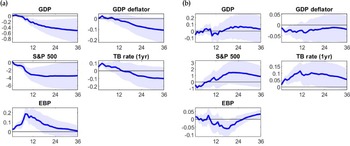
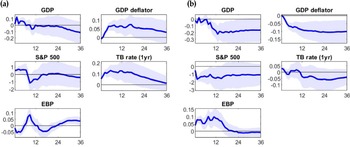
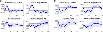
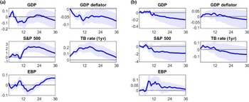
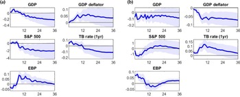
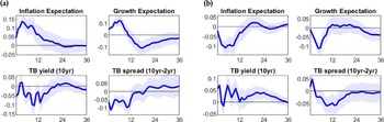
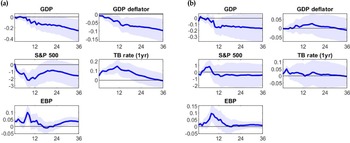
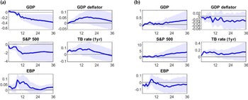
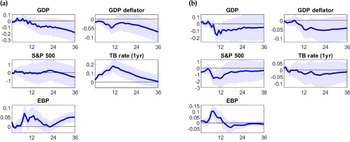
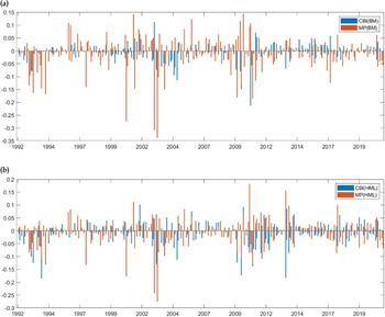


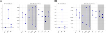


 Open access

