


1. Introduction
Huge losses in properties, motor vehicles, and from the interruption of businesses occur due to conventional catastrophic events, such as flood, storm, hail, bushfire, earthquake, terrorism, and global war. Emerging cyber and pandemic events bring about catastrophic and far-reaching losses from business interruption.
The estimated cost of claims related to the February and March 2022 South-East Queensland and New South Wales floods, which is the third most costly extreme weather event ever recorded in Australia, by the Insurance Council of Australia (ICA) is AU$4.8 billion. Insurers’ losses from October 2022 Hurricane Ian, one of the most powerful storms ever recorded in the US, are expected to be between US$42 billion and US$57 billion. In July 2023, we have seen extreme weather events, i.e., floods in Asia, wildfires in Canada, and deadly heatwaves in southern Europe and the US, which can impact economies badly with huge financial costs.
Hurricane Helene slammed into Florida’s Gulf Coast, causing deadly flooding and dumping almost unprecedented amounts of rain in September 2024. AccuWeather Inc. estimated that total damage and economic loss could be between US$145 billion and US$160 billion. Spain has been affected by record-breaking rainfall and severe flooding in Valencia in late October 2024. The Southern California wildfires of January 2025 illustrate the dynamics of claims. Moody’s Risk Management Solutions (RMS) event response estimates that insured losses for Los Angeles firestorm events will likely range between US$20 billion and US$30 billion. These events present significant challenges to the financial stability of insurers and reinsurers, highlighting the need for improved models to predict claims from catastrophic events.
In May 2021 a ransomware cyberattack halted the US Colonial Pipeline by disrupting its computerized control systems. Nearly half of the US East Coast’s fuel supply depends on this pipeline, which transports gasoline, diesel, jet fuel, and other refined products. The Colonial Pipeline Company acknowledged that it paid a ransom of US$4.4 million worth of bitcoin, though the US Department of Justice was able to recover 64 bitcoins worth US$2.3 million. According to the Travel, Logistics & Infrastructure article, airlines suffered $168 billion in economic losses in 2020, although the COVID-19 pandemic was entering its endemic stages in some parts of the world (Bouwer et al., Reference Bouwer, Krishnan and Tufft2022).
Insurers provide coverage to individuals and organizations by underwriting policies that protect against economic and financial losses resulting from catastrophic events. However, insurers cannot cover all losses, as extreme risks pose a challenge to their financial viability. To ensure solvency in case of exceptionally huge losses, insurers transfer their risk portfolios by purchasing catastrophe reinsurance contracts.
The frequency and severity of both conventional and emerging catastrophes are increasing due to factors such as global warming, cyberattacks, and pandemics. Gürtler et al. (Reference Gürtler, Hibbeln and Winkelvos2016) observed that insurance premiums rose significantly following natural mega-catastrophes to mitigate the risk of financial losses for reinsurers. In March 2024, prior to the Southern California wildfires of January 2025, State Farm, the largest property insurer in the US, announced that it would not renew insurance policies in high-risk California postcodes due to escalating costs, including rising reinsurance premiums and construction expenses.
As a result, alternative point processes are needed to model claim and loss arrivals from both conventional and emerging catastrophic events, ensuring effective pricing of catastrophe insurance and reinsurance contracts. To articulate the ongoing challenge and complexity of new risk dynamics, we use a compound dynamic contagion process (CDCP) (Dassios & Zhao, Reference Dassios and Zhao2011) for the catastrophic component of the liability of a reinsurer (i.e., the aggregate catastrophe loss covered by a reinsurance contract), denoted by $C_{t}$
. This makes our study unique, and to our knowledge, using it for the catastrophic component of the liability of
$C_{t}$
. This makes our study unique, and to our knowledge, using it for the catastrophic component of the liability of $C_{t}$
is the first contribution in the context of pricing for a catastrophe reinsurance contract. For references on this compound point process, we refer to Jang and Oh (Reference Jang and Oh2021) and relevant citations therein. Recently, Liu and Jang (Reference Liu and Jang2025) applied enhanced dynamic contagion processes to study optimal asset allocation and reinsurance problems.
$C_{t}$
is the first contribution in the context of pricing for a catastrophe reinsurance contract. For references on this compound point process, we refer to Jang and Oh (Reference Jang and Oh2021) and relevant citations therein. Recently, Liu and Jang (Reference Liu and Jang2025) applied enhanced dynamic contagion processes to study optimal asset allocation and reinsurance problems.
The CDCP is particularly well suited to modeling catastrophe reinsurance liabilities because its probabilistic structure directly reflects key empirical features of catastrophic loss arrivals. First, the self-exciting component captures claim clustering and loss amplification, which are often observed after major catastrophes. Specifically, an initial event (e.g., a severe flood or wildfire) generates subsequent related claims through infrastructure damage, supply-chain disruption, or aftershocks. Second, the external-excitation component allows for sudden exogenous shocks, such as hurricanes, pandemics, or cyber events, whose arrival times are not triggered by past insurance losses but by external environmental or systemic factors. Third, the mean-reverting intensity ensures that periods of elevated risk eventually decay, consistent with the transient nature of catastrophe-driven claim activities.
To ensure risk-neutrality, we use an equivalent martingale probability measure $\tilde {\mathbb{P}}$
for the compound dynamic contagion process
$\tilde {\mathbb{P}}$
for the compound dynamic contagion process $C_{t}$
, derived using the Esscher transform, to evaluate an arbitrage-free premium. In the field of actuarial science, risk-neutral pricing via the Esscher transform (Esscher, Reference Esscher1932) can be found, for example, in Gerber and Shiu (Reference Gerber and Shiu1994), Gerber and Shiu (Reference Gerber and Shiu1996), Bühlmann et al. (Reference Bühlmann, Delbaen, Embrechts and Shiryaev1996), Dassios and Jang (Reference Dassios and Jang2003), Jang and Krvavych (Reference Jang and Krvavych2004), Siu et al. (Reference Siu, Tong and Yang2004), and Siu (Reference Siu2005).
$C_{t}$
, derived using the Esscher transform, to evaluate an arbitrage-free premium. In the field of actuarial science, risk-neutral pricing via the Esscher transform (Esscher, Reference Esscher1932) can be found, for example, in Gerber and Shiu (Reference Gerber and Shiu1994), Gerber and Shiu (Reference Gerber and Shiu1996), Bühlmann et al. (Reference Bühlmann, Delbaen, Embrechts and Shiryaev1996), Dassios and Jang (Reference Dassios and Jang2003), Jang and Krvavych (Reference Jang and Krvavych2004), Siu et al. (Reference Siu, Tong and Yang2004), and Siu (Reference Siu2005).
This paper considers the fair valuation of catastrophe stop-loss reinsurance contracts. We arrange the paper as follows. In section 2, we provide a mathematical definition for the CDCP for $C_{t}$
, which was introduced by Jang and Oh (Reference Jang and Oh2021). The infinitesimal generator of the joint process is also provided, extending it to the time-inhomogeneous case, together with required moments. We describe our insurance market and discuss the condition of the absence of arbitrage in Section 3. Section 4 provides arbitrage-free catastrophe reinsurance premiums numerically obtained using the Monte Carlo simulation method. Comparisons are also made with the generalized Hawkes case and the Cox case, respectively. Sensitivity analyses are performed by changing the retention level, the Esscher parameters, and the intensity parameters. Section 5 concludes the paper. Appendix A defines an equivalent martingale measure under a non-zero interest rate, while Appendix B details our Monte Carlo algorithms.
$C_{t}$
, which was introduced by Jang and Oh (Reference Jang and Oh2021). The infinitesimal generator of the joint process is also provided, extending it to the time-inhomogeneous case, together with required moments. We describe our insurance market and discuss the condition of the absence of arbitrage in Section 3. Section 4 provides arbitrage-free catastrophe reinsurance premiums numerically obtained using the Monte Carlo simulation method. Comparisons are also made with the generalized Hawkes case and the Cox case, respectively. Sensitivity analyses are performed by changing the retention level, the Esscher parameters, and the intensity parameters. Section 5 concludes the paper. Appendix A defines an equivalent martingale measure under a non-zero interest rate, while Appendix B details our Monte Carlo algorithms.
2. Dynamics for catastrophe losses
In this section, the dynamics for catastrophe losses from the insurer/reinsurer’s perspective are described. Specifically, a dynamic contagion process (DCP) with a stochastic intensity process is adopted to model the number of catastrophes. Indeed, from the reinsurer’s perspective, the catastrophic component of the liability is given by the aggregate catastrophic losses to be covered by a reinsurance contract. The aggregate catastrophic losses are described by a CDCP.
2.1 Dynamic contagion process
A definition for the standard DCP with time-homogeneous parameters will be provided by Definition 1, while a definition for the associated CDCP will be provided by Definition 2. We will extend it to a version with time-inhomogeneous parameters later.
We start with a complete probability space $(\Omega , \mathcal{F},\mathbb{P})$
, where
$(\Omega , \mathcal{F},\mathbb{P})$
, where $\mathbb{P}$
is a real-world probability measure, which is called a physical probability measure. Suppose that the probability space
$\mathbb{P}$
is a real-world probability measure, which is called a physical probability measure. Suppose that the probability space $(\Omega , \mathcal{F},\mathbb{P})$
is sufficiently rich to allow for the definition of all the random processes or quantities that will be introduced subsequently. A continuous-time model with a finite horizon
$(\Omega , \mathcal{F},\mathbb{P})$
is sufficiently rich to allow for the definition of all the random processes or quantities that will be introduced subsequently. A continuous-time model with a finite horizon $\mathcal{T} \, :\!= \, [0, T]$
is considered, where
$\mathcal{T} \, :\!= \, [0, T]$
is considered, where $T \lt \infty$
. Let
$T \lt \infty$
. Let $\{ N_t \}_{t \in \mathcal{T}}$
denote a point process defined on
$\{ N_t \}_{t \in \mathcal{T}}$
denote a point process defined on $(\Omega , \mathcal{F},\mathbb{P})$
. Let
$(\Omega , \mathcal{F},\mathbb{P})$
. Let $\{ T_{2, j} \}_{j = 1, 2, \ldots }$
be a sequence of random jump times of the point process
$\{ T_{2, j} \}_{j = 1, 2, \ldots }$
be a sequence of random jump times of the point process $\{ N_t \}_{t \in \mathcal{T}}$
. That is,
$\{ N_t \}_{t \in \mathcal{T}}$
. That is, $\{ T_{2, j} \}_{j = 1, 2, \ldots }$
is a sequence of positive-valued random variables on
$\{ T_{2, j} \}_{j = 1, 2, \ldots }$
is a sequence of positive-valued random variables on $(\Omega , \mathcal{F},\mathbb{P})$
such that
$(\Omega , \mathcal{F},\mathbb{P})$
such that $0 \lt T_{2, 1} \lt T_{2, 2} \lt \cdots$
,
$0 \lt T_{2, 1} \lt T_{2, 2} \lt \cdots$
, $\mathbb{P}$
-a.s. Then, for all
$\mathbb{P}$
-a.s. Then, for all $t \in \mathcal{T}$
,
$t \in \mathcal{T}$
,
 \begin{align*} N_t = \sum _{j \ge 1} \mathbb{I}_{\{ T_{2, j} \le t \} }, \end{align*}
where $\mathbb{I}_A$
is the indicator function of an event
$\mathbb{I}_A$
is the indicator function of an event $A$
.
$A$
.
Write $\{ Y_j \}_{j = 1, 2, \ldots }$
for the random positive jump sizes corresponding to the random jump times
$\{ Y_j \}_{j = 1, 2, \ldots }$
for the random positive jump sizes corresponding to the random jump times $\{ T_{2, j} \}_{j = 1, 2, \ldots }$
. Specifically, for each
$\{ T_{2, j} \}_{j = 1, 2, \ldots }$
. Specifically, for each $j = 1, 2, \ldots$
,
$j = 1, 2, \ldots$
, $Y_j$
is the random positive jump size corresponding to the random jump time
$Y_j$
is the random positive jump size corresponding to the random jump time $T_{2, j}$
. Assume that
$T_{2, j}$
. Assume that $\{ Y_j \}_{j = 1, 2, \ldots }$
is a sequence of independent and identically distributed (i.i.d.) positive random variables on
$\{ Y_j \}_{j = 1, 2, \ldots }$
is a sequence of independent and identically distributed (i.i.d.) positive random variables on $(\Omega , \mathcal{F}, \mathbb{P})$
with the common distribution
$(\Omega , \mathcal{F}, \mathbb{P})$
with the common distribution $G (y)$
, where
$G (y)$
, where $y \gt 0$
.
$y \gt 0$
.
Let $\{ M_t \}_{t \in \mathcal{T}}$
be a Poisson point process on
$\{ M_t \}_{t \in \mathcal{T}}$
be a Poisson point process on $(\Omega , \mathcal{F},\mathbb{P})$
such that its intensity process is given by
$(\Omega , \mathcal{F},\mathbb{P})$
such that its intensity process is given by $\rho \gt 0$
, for all
$\rho \gt 0$
, for all $t \in \mathcal{T}$
,
$t \in \mathcal{T}$
, $\mathbb{P}$
-a.s. Write
$\mathbb{P}$
-a.s. Write $\{ T_{1, i} \}_{i = 1, 2, \ldots }$
and
$\{ T_{1, i} \}_{i = 1, 2, \ldots }$
and $\{ X_i \}_{i = 1, 2, \ldots }$
for the random jump times and sizes for the Poisson point process
$\{ X_i \}_{i = 1, 2, \ldots }$
for the random jump times and sizes for the Poisson point process $\{ M_t \}_{t \in \mathcal{T}}$
, respectively. Again, suppose that
$\{ M_t \}_{t \in \mathcal{T}}$
, respectively. Again, suppose that $\{ X_i \}_{i = 1, 2, \ldots }$
is a sequence of i.i.d. positive random variables on
$\{ X_i \}_{i = 1, 2, \ldots }$
is a sequence of i.i.d. positive random variables on $(\Omega , \mathcal{F}, \mathbb{P})$
with the common distribution
$(\Omega , \mathcal{F}, \mathbb{P})$
with the common distribution $H(x)$
, where
$H(x)$
, where $x \gt 0$
. Assume that under the probability measure
$x \gt 0$
. Assume that under the probability measure $\mathbb{P}$
,
$\mathbb{P}$
, $\{ X_i \}_{i = 1, 2, \ldots }$
,
$\{ X_i \}_{i = 1, 2, \ldots }$
, $\{ T_{1,i} \}_{i = 1, 2, \ldots }$
, and
$\{ T_{1,i} \}_{i = 1, 2, \ldots }$
, and $\{ Y_{j} \}_{j = 1, 2, \ldots }$
are independent of each other.
$\{ Y_{j} \}_{j = 1, 2, \ldots }$
are independent of each other.
Definition 1 (Dynamic contagion process). Suppose the point process $\{ N_t \}_{t \in \mathcal{T}}$
has a stochastic intensity process
$\{ N_t \}_{t \in \mathcal{T}}$
has a stochastic intensity process $\{ \lambda _t \}_{t \in \mathcal{T}}$
under the probability measure
$\{ \lambda _t \}_{t \in \mathcal{T}}$
under the probability measure $\mathbb{P}$
. Then
$\mathbb{P}$
. Then $\{ N_t \}_{t \in \mathcal{T}}$
is said to be a DCP if
$\{ N_t \}_{t \in \mathcal{T}}$
is said to be a DCP if $\{ \lambda _t \}_{t \in \mathcal{T}}$
is given by:
$\{ \lambda _t \}_{t \in \mathcal{T}}$
is given by:
 \begin{equation} \lambda _{t} = a + \left ( \lambda _{0}-a\right ) \mathrm{e}^{-\delta t}+\sum _{i \ge 1} X_{i} \mathrm{e}^{-\delta \left ( t - T_{1, i} \right )}\mathbb{I}_{\{ T_{1,i} \le t \}} + \sum _{j \ge 1} Y_{j} \mathrm{e}^{-\delta \left (t - T_{2,j} \right )} \mathbb{I}_{ \{ T_{2, j} \le t \}}, \end{equation}
where
-
• the constant mean-reverting (baseline) intensity level $a \ge 0$
;
$a \ge 0$
; -
• the constant initial intensity at time
$t = 0$
,
$\lambda _{0} \geq a$
,
$\mathbb{P}$
-a.s.;
-
• the constant rate of exponential decay
$\delta \gt 0$
.


In Definition 1, $\left \{ X_{i}\right \}_{i=1,2,\ldots }$
is interpreted as a sequence of positive externally-excited jumps, while
$\left \{ X_{i}\right \}_{i=1,2,\ldots }$
is interpreted as a sequence of positive externally-excited jumps, while $\left \{ Y_{j}\right \}_{j=1,2,\ldots }$
is interpreted as a sequence of positive self-excited jumps. If there are no externally excited jumps in Eq. (2.1) (i.e.,
$\left \{ Y_{j}\right \}_{j=1,2,\ldots }$
is interpreted as a sequence of positive self-excited jumps. If there are no externally excited jumps in Eq. (2.1) (i.e., $\rho =0$
for all
$\rho =0$
for all $t \in \mathcal{T}$
)
$t \in \mathcal{T}$
) $\{ N_{t} \}_{t \in \mathcal{T}}$
becomes a generalized Hawkes process. If
$\{ N_{t} \}_{t \in \mathcal{T}}$
becomes a generalized Hawkes process. If $a=0$
and there are no self-excited jumps in Eq. (2.1),
$a=0$
and there are no self-excited jumps in Eq. (2.1), $\{ N_{t} \}_{t \in \mathcal{T}}$
becomes the Cox process with shot-noise Poisson intensity. It may be noted that these processes are within the general framework of affine processes. See, for example, Duffie et al. (Reference Duffie, Pan and Singleton2000, Reference Duffie, Filipovic and Schachermayer2003) and Glasserman and Kim (Reference Glasserman and Kim2010). Let
$\{ N_{t} \}_{t \in \mathcal{T}}$
becomes the Cox process with shot-noise Poisson intensity. It may be noted that these processes are within the general framework of affine processes. See, for example, Duffie et al. (Reference Duffie, Pan and Singleton2000, Reference Duffie, Filipovic and Schachermayer2003) and Glasserman and Kim (Reference Glasserman and Kim2010). Let $\mathbb{F}^{\lambda }$
and
$\mathbb{F}^{\lambda }$
and $\mathbb{F}^N$
denote the
$\mathbb{F}^N$
denote the $\mathbb{P}$
-augmentation of the natural filtration generated by the stochastic intensity process
$\mathbb{P}$
-augmentation of the natural filtration generated by the stochastic intensity process $\{ \lambda _t \}_{t \in \mathcal{T}}$
and the point process
$\{ \lambda _t \}_{t \in \mathcal{T}}$
and the point process $\{ N_t \}_{t \in \mathcal{T}}$
, respectively. That is,
$\{ N_t \}_{t \in \mathcal{T}}$
, respectively. That is, $\mathbb{F}^{\lambda } \, :\!= \, \{ \mathcal{F}^{\lambda }_t \}_{t \in \mathcal{T}}$
and
$\mathbb{F}^{\lambda } \, :\!= \, \{ \mathcal{F}^{\lambda }_t \}_{t \in \mathcal{T}}$
and $\mathbb{F}^N \, :\!= \, \{ \mathcal{F}^N_t \}_{t \in \mathcal{T}}$
so that for all
$\mathbb{F}^N \, :\!= \, \{ \mathcal{F}^N_t \}_{t \in \mathcal{T}}$
so that for all $t \in \mathcal{T}$
,
$t \in \mathcal{T}$
,
 \begin{equation*} \begin{aligned} \mathcal{F}^{\lambda }_t &\, :\!= \, \sigma \{ \lambda _u \,|\, u \in [0, t] \} \vee \mathcal{N}, \\ \mathcal{F}^N_t &\, :\!= \, \sigma \{ N_u \,|\, u \in [0, t] \} \vee \mathcal{N}, \end{aligned} \end{equation*}
where $\mathcal{N}$
is a collection of the
$\mathcal{N}$
is a collection of the $\mathbb{P}$
-null subsets of
$\mathbb{P}$
-null subsets of $\mathcal{F}$
;
$\mathcal{F}$
; $\mathcal{F}_1 \vee \mathcal{F}_2$
is the minimal
$\mathcal{F}_1 \vee \mathcal{F}_2$
is the minimal $\sigma$
-field containing the two
$\sigma$
-field containing the two $\sigma$
-fields
$\sigma$
-fields $\mathcal{F}_1$
and
$\mathcal{F}_1$
and $\mathcal{F}_2$
. Note that for all
$\mathcal{F}_2$
. Note that for all $t \in \mathcal{T}$
,
$t \in \mathcal{T}$
, $\mathcal{F}^N_t \subset \mathcal{F}^{\lambda }_t$
.
$\mathcal{F}^N_t \subset \mathcal{F}^{\lambda }_t$
.
2.2 Compound dynamic contagion process
This section provides a definition of the CDCP that will be used for the catastrophic component of the liability. We also provide the infinitesimal generator of this process and relevant moments, after which we deal with it separately when the parameters of this process are time-inhomogeneous.
Definition 2 (Dynamic contagion claims). Suppose $\{ T_{2, j} \}_{j = 1, 2, \ldots }$
is a sequence of random jump times of the DCP
$\{ T_{2, j} \}_{j = 1, 2, \ldots }$
is a sequence of random jump times of the DCP $\{ N_t \}_{t \in \mathcal{T}}$
having the stochastic intensity process
$\{ N_t \}_{t \in \mathcal{T}}$
having the stochastic intensity process $\{ \lambda _t \}_{t \in \mathcal{T}}$
given by Eq. (
2.1
). Let
$\{ \lambda _t \}_{t \in \mathcal{T}}$
given by Eq. (
2.1
). Let $\{ \Xi _{j} \}_{j = 1, 2, \ldots }$
be a sequence of i.i.d. positive individual loss amounts with the common distribution function
$\{ \Xi _{j} \}_{j = 1, 2, \ldots }$
be a sequence of i.i.d. positive individual loss amounts with the common distribution function $J(\xi )$
, where
$J(\xi )$
, where $\xi \gt 0$
such that for each
$\xi \gt 0$
such that for each $j = 1, 2, \ldots$
,
$j = 1, 2, \ldots$
, $\Xi _j$
is the individual loss amount that occurs at random time
$\Xi _j$
is the individual loss amount that occurs at random time $T_{2, j}$
. Assume that under the probability measure
$T_{2, j}$
. Assume that under the probability measure $\mathbb{P}$
,
$\mathbb{P}$
, $\left \{ X_{i}\right \}_{i=1,2,\ldots }$
,
$\left \{ X_{i}\right \}_{i=1,2,\ldots }$
, $\left \{ T_{1,i}\right \}_{i=1,2,\ldots }$
,
$\left \{ T_{1,i}\right \}_{i=1,2,\ldots }$
, $\left \{ Y_{j}\right \}_{j=1,2,\ldots }$
and
$\left \{ Y_{j}\right \}_{j=1,2,\ldots }$
and $\left \{ \Xi _{j}\right \}_{j=1,2,\ldots }$
are independent of each other. Then a compound point process
$\left \{ \Xi _{j}\right \}_{j=1,2,\ldots }$
are independent of each other. Then a compound point process $\{ C_t \}_{t \in \mathcal{T}}$
is said to be a CDCP if
$\{ C_t \}_{t \in \mathcal{T}}$
is said to be a CDCP if
 \begin{align*} C_{t}=\sum \limits _{j\geq 1}\Xi _{j}\mathbb{I}_{\{ T_{2,j} \le t \} }. \\[-20pt] \end{align*}
Let us denote the integrated intensity process
 \begin{equation*} {\Lambda _t \,\, :\!= \,\, \int ^t_0 \lambda _u \mathop {}\!\mathrm{d} u}. \end{equation*}
2.2.1 Time-homogeneous compound dynamic contagion process
For the standard DCP with time-homogeneous parameters, the infinitesimal generator $\mathcal{A}$
of the joint process
$\mathcal{A}$
of the joint process $\{ \left ( \lambda _{t},N_{t},C_{t}, {M_t}, {\Lambda _t}, t\right ) \}_{t \in \mathcal{T}}$
acting on a function
$\{ \left ( \lambda _{t},N_{t},C_{t}, {M_t}, {\Lambda _t}, t\right ) \}_{t \in \mathcal{T}}$
acting on a function $f(\lambda ,n,c,{m},{\Lambda },t)\in \mathcal{D}( \mathcal{A} )$
is given by:
$f(\lambda ,n,c,{m},{\Lambda },t)\in \mathcal{D}( \mathcal{A} )$
is given by:
 \begin{align} &\hspace {-0.5cm}\mathcal{A} f( \lambda , n,c,{m}, {\Lambda }, t) \notag \\ &= \frac {\partial f}{\partial t}+\delta \left ( a-\lambda \right ) \frac {\partial f}{\partial \lambda } + {\lambda \frac {\partial f}{\partial \Lambda }} \notag \\ &\quad +\lambda \left [ \int _{0}^{\infty }\int _{0}^{\infty }f( \lambda +y,n+1,c+\xi ,{m},{\Lambda },t) \mathop {}\!\mathrm{d} G(y)\mathop {}\!\mathrm{d} J(\xi )-f( \lambda ,n,c,{m},{\Lambda },t) \right ] \notag \\ &\quad +\rho \left [ \int _{0}^{\infty }f( \lambda +x,n,c,{m+1},{\Lambda },t) \mathop {}\!\mathrm{d} H(x)-f( \lambda ,n,c,{m},{\Lambda },t) \right ]\!, \end{align}
where $\mathcal{D}( \mathcal{A})$
is the domain of the generator
$\mathcal{D}( \mathcal{A})$
is the domain of the generator $\mathcal{A}$
such that
$\mathcal{A}$
such that $f(\lambda ,n,c,{m},{\Lambda },t)$
is differentiable with respect to
$f(\lambda ,n,c,{m},{\Lambda },t)$
is differentiable with respect to $\lambda$
and
$\lambda$
and $t$
, and
$t$
, and
 \begin{equation*} \left \vert \int _{0}^{\infty }\int _{0}^{\infty }f( \lambda +y,n+1,c+\xi ,{m},{\Lambda },t) \mathop {}\!\mathrm{d} G(y)\mathop {}\!\mathrm{d} J(\xi )-f( \lambda ,n,c,{m},{\Lambda },t) \right \vert \lt \infty \text{,} \end{equation*}
 \begin{equation*} \left \vert \int _{0}^{\infty }f( \lambda +x,n,c,{m+1},{\Lambda },t) \mathop {}\!\mathrm{d} H(x)-f( \lambda ,n,c,{m},{\Lambda },t) \right \vert \lt \infty \text{.} \end{equation*}
For details on the definition and derivations of the infinitesimal generator in (2.2), please refer to Dassios and Zhao (Reference Dassios and Zhao2011), Dassios and Zhao (Reference Dassios and Zhao2017), Jang and Oh (Reference Jang and Oh2021), and Øksendal (Reference Øksendal2013).
Based on Eq. (2.2), we can easily obtain the moments of $\lambda _t$
,
$\lambda _t$
, $N_t$
, and
$N_t$
, and $C_{t}$
. To do so, we denote the first-order moments of
$C_{t}$
. To do so, we denote the first-order moments of $X$
,
$X$
, $Y$
, and
$Y$
, and $\Xi$
, respectively, by
$\Xi$
, respectively, by
 \begin{equation*} {\mu _{H}=\int _{0}^{\infty }x \mathop {}\!\mathrm{d} H(x)},\ \ \mu _{G}=\int _{0}^{\infty }y \mathop {}\!\mathrm{d} G(y),\ \ \mu _{J}=\int _{0}^{\infty }\xi \mathop {}\!\mathrm{d} J(\xi ) . \end{equation*}
and their Laplace transforms by
 \begin{equation} {\hat {h}(s) = \int _{0}^{\infty }\mathrm{e}^{-s x} \mathop {}\!\mathrm{d} H(x)}, \quad \hat {g}(s) = \int _{0}^{\infty }\mathrm{e}^{-s y} \mathop {}\!\mathrm{d} G(y), \quad \hat {j}(s) = \int _{0}^{\infty }\mathrm{e}^{-s \xi }\mathop {}\!\mathrm{d} J(\xi ), \end{equation}
which are supposed to be finite. The Laplace transforms will be used in Section 3.
The following proposition for a standard CDCP with time-homogeneous parameters is directly adapted from Dassios and Zhao (Reference Dassios and Zhao2011); Dassios and Zhao (Reference Dassios and Zhao2017) and Jang and Oh (Reference Jang and Oh2021).
Proposition 1 (Expectations of $\lambda _t$
,
$\lambda _t$
, $N_t$
, and
$N_t$
, and $C_t$
for time-homogeneous CDCP). The expectation of
$C_t$
for time-homogeneous CDCP). The expectation of $\lambda _{t}$
conditional on
$\lambda _{t}$
conditional on $\lambda _0$
under the real-world probability measure
$\lambda _0$
under the real-world probability measure $\mathbb{P}$
is given by
$\mathbb{P}$
is given by
 \begin{equation*} \mathbb{E}\left [ \lambda _{t} \mid \lambda _0 \right ] \,=\, \left \{ \begin{array}{ll} \dfrac {\rho \mu _H + a\delta }{\kappa } + \left ( \lambda _0 - \dfrac {\rho \mu _H + a\delta }{\kappa } \right ) \mathrm{e}^{-\kappa t}, &\quad \kappa \neq 0,\\ \lambda _0 + \left (\rho \mu _H+ a\delta \right )t, &\quad \kappa =0, \end{array} \right . \end{equation*}
where $\kappa \, :\!= \, \delta - \mu _{G}$
. Under the stationary condition
$\kappa \, :\!= \, \delta - \mu _{G}$
. Under the stationary condition $\kappa \gt 0$
, the asymptotic first moment of
$\kappa \gt 0$
, the asymptotic first moment of $\lambda _{t}$
under
$\lambda _{t}$
under $\mathbb{P}$
is given by
$\mathbb{P}$
is given by
 \begin{equation*} \mu _1\ \, :\!= \,\ \lim _{t\rightarrow \infty }\mathbb{E}\left [ \lambda _{t} \mid \lambda _0 \right ] \ =\ \frac {\rho \mu _H + a\delta }{\kappa }. \end{equation*}
The expectation of $N_{t}$
conditional on
$N_{t}$
conditional on $N_0=0$
and
$N_0=0$
and $\lambda _0$
under
$\lambda _0$
under $\mathbb{P}$
is given by
$\mathbb{P}$
is given by
 \begin{equation*} \mathbb{E}\left [ N_{t} \mid \lambda _0 \right ] \,=\, \left \{ \begin{array}{ll} \mu _1 t + \left ( \lambda _0 - \mu _1 \right ) \dfrac {1}{ \kappa } ( 1-\mathrm{e}^{- \kappa t} ), &\quad \kappa \neq 0,\\ \lambda _0 t + \dfrac {1}{2}\left (\rho \mu _H+ a\delta \right ){t^2}, &\quad \kappa = 0. \end{array} \right . \end{equation*}
The expectation of $C_{t}$
conditional on
$C_{t}$
conditional on $C_0=0$
and
$C_0=0$
and $\lambda _0$
under
$\lambda _0$
under $\mathbb{P}$
is given by
$\mathbb{P}$
is given by
 \begin{equation*} \mathbb{E}\left [ C_{t} \mid \lambda _0 \right ] \,=\, \left \{ \begin{array}{ll} \mu _J \left[ \mu _1 t + \left ( \lambda _0 - \mu _1 \right ) \dfrac {1}{ \kappa } ( 1-\mathrm{e}^{- \kappa t} ) \right]\!, &\quad \kappa \neq 0,\\[8pt] \mu _J \left[ \lambda _0 t + \dfrac {1}{2} {\left (\rho \mu _H+ a\delta \right )}{t^2 }\right]\!, &\quad \kappa = 0. \end{array} \right . \end{equation*}
2.2.2 Time-inhomogeneous compound dynamic contagion process
The previously defined DCP $\lambda _t$
from Eq. (2.1) is the result of solving the stochastic differential equation (SDE)
$\lambda _t$
from Eq. (2.1) is the result of solving the stochastic differential equation (SDE)
 \begin{equation} \lambda _{t} = \lambda _0 + \int _{0}^{t} \delta \left ( a - \lambda _s \right ) \mathop {}\!\mathrm{d} s + \sum _{i \ge 1} X_{i} \, \mathbb{I}_{\{ T_{1,i} \le t \}} + \sum _{j \ge 1} Y_{j} \, \mathbb{I}_{ \{ T_{2, j} \le t \}} . \end{equation}
The parameters of this process are all time-homogeneous. More generally, we can extend to the time-inhomogeneous situation by allowing the parameters to vary over time (except the decaying rate $\delta$
). Specifically, we impose the following assumptions:
$\delta$
). Specifically, we impose the following assumptions:
-
(A1) The mean-reverting level
$a(t)$
and the rate of externally excited jump arrival
$\rho (t)$
are deterministic functions of time
$t$
; they are bounded on all intervals
$[0, t)$
(no explosions); and
$\lambda _0 \geq a(t)$
. -
(A2) The distribution function of the externally excited jump sizes at any time
$t$
is
$H(x; \, t)$
for
$x \gt 0$
with
$\mu _H(t) = \int _0^\infty x \, \mathop {}\!\mathrm{d} H(x; \, t)$
. -
(A3) The distribution function of the self-excited jump sizes at any time
$t$
is
$G(y; \, t)$
for
$y \gt 0$
with
$\mu _G(t) = \int _0^\infty y \, \mathop {}\!\mathrm{d} G(y; \, t)$
. -
(A4)
$a(t)$
,
$\rho (t)$
,
$G(y; \, t)$
and
$H(x; \, t)$
are Riemann-integrable functions of
$t$
; they are all positive.








After replacing the time-homogeneous constants in Eq. (2.4) with time-varying functions and solving the SDE, we arrive at the $\lambda _t$
for this new time-inhomogeneous DCP
$\lambda _t$
for this new time-inhomogeneous DCP
 \begin{equation} \lambda _{t} = \lambda _0 \mathrm{e}^{-\delta t} + \delta \int _{0}^{t} a(s) \mathrm{e}^{-\delta (t-s)} \, \mathop {}\!\mathrm{d} s + \sum _{i \ge 1} X_{i} \mathrm{e}^{-\delta \left ( t - T_{1, i} \right )}\mathbb{I}_{\{ T_{1,i} \le t \}} + \sum _{j \ge 1} Y_{j} \mathrm{e}^{-\delta \left (t - T_{2,j} \right )} \mathbb{I}_{ \{ T_{2, j} \le t \}}. \end{equation}
We allow the model parameters to be time-inhomogeneous or time-varying to reflect evolving exposure and claim dynamics in the insurance and reinsurance portfolios. Specifically, in reality, claim intensity and contagion effects may vary over time due to changes in insured exposure, portfolio composition, seasonal effects, and external risk conditions. Introducing time-inhomogeneity at this stage provides a flexible actuarial framework for modeling claim arrivals, while its role under an equivalent change of measures will become apparent later in Section 3.
For this time-inhomogeneous CDCP, we can obtain the moments of $\lambda _t$
,
$\lambda _t$
, $N_t$
, and
$N_t$
, and $C_t$
as below, where the relevant parameters are time-dependent. They extend the results in Proposition 1.
$C_t$
as below, where the relevant parameters are time-dependent. They extend the results in Proposition 1.
Proposition 2 (Expectations of $\lambda _t$
,
$\lambda _t$
, $N_t$
, and
$N_t$
, and $C_t$
for time-inhomogeneous CDCP). For the time-inhomogeneous CDCP, the expectation of
$C_t$
for time-inhomogeneous CDCP). For the time-inhomogeneous CDCP, the expectation of $\lambda _t$
conditional on
$\lambda _t$
conditional on $\lambda _0$
under the real-world probability measure
$\lambda _0$
under the real-world probability measure $\mathbb{P}$
is given by
$\mathbb{P}$
is given by
 \begin{equation} \mu _{\lambda }(t) \,\, :\!= \,\, \mathbb{E}\left [ \lambda _{t}\mid \lambda _{0}\right ] \,=\, \lambda _{0} \mathrm{e}^{-\int _{0}^{t} \kappa (s) \mathop {}\!\mathrm{d} s} + \mathrm{e}^{-\int _{0}^{t} \kappa (s) \mathop {}\!\mathrm{d} s} \int \limits _{0}^{t} \mathrm{e}^{\int _{0}^{s} \kappa (u) \mathop {}\!\mathrm{d} u} \big \{ \rho (s) \mu _H(s)+a(s) \delta \big \} \mathop {}\!\mathrm{d} s, \end{equation}
where
 \begin{equation*} \kappa (t) \, :\!= \, \delta - \mu _G(t). \end{equation*}
The expectation of $N_{t}$
conditional on
$N_{t}$
conditional on $N_0=0$
and
$N_0=0$
and $\lambda _0$
under
$\lambda _0$
under $\mathbb{P}$
is given by
$\mathbb{P}$
is given by
 \begin{equation} \mathbb{E}[ N_{t} \mid \lambda _{0} ] = \int \limits _{0}^{t} \mu _{\lambda }(s) \mathop {}\!\mathrm{d} s. \end{equation}
The expectation of $C_{t}$
conditional on
$C_{t}$
conditional on $C_0=0$
and
$C_0=0$
and $\lambda _0$
under
$\lambda _0$
under $\mathbb{P}$
is given by
$\mathbb{P}$
is given by
 \begin{equation} \mathbb{E}[ C_{t} \mid \lambda _{0} ] = \mu _{J} \int \limits _{0}^{t} \mu _{\lambda }(s) \mathop {}\!\mathrm{d} s. \end{equation}
Proof.
The infinitesimal generator $\mathcal{A}$
of the joint process
$\mathcal{A}$
of the joint process $\{ \left ( \lambda _{t},N_{t},C_{t}, {M_t}, {\Lambda _t}, t\right ) \}_{t \in \mathcal{T}}$
acting on a function
$\{ \left ( \lambda _{t},N_{t},C_{t}, {M_t}, {\Lambda _t}, t\right ) \}_{t \in \mathcal{T}}$
acting on a function $ f(\lambda ,n,c,{m},{\Lambda },t)\in \mathcal{D}\left ( \mathcal{A} \right )$
for the time-inhomogeneous CDCP is given by:
$ f(\lambda ,n,c,{m},{\Lambda },t)\in \mathcal{D}\left ( \mathcal{A} \right )$
for the time-inhomogeneous CDCP is given by:
 \begin{align} &\hspace {-0.5cm}\mathcal{A} f( \lambda , n,c,{m}, {\Lambda }, t) \notag \\ &= \frac {\partial f}{\partial t}+\delta \big ( a(t)-\lambda \big ) \frac {\partial f}{\partial \lambda } + {\lambda \frac {\partial f}{\partial \Lambda }} \notag \\ &\quad +\lambda \left [ \int _{0}^{\infty }\int _{0}^{\infty }f( \lambda +y,n+1,c+\xi ,{m},{\Lambda },t) \mathop {}\!\mathrm{d} G(y; \, t)\mathop {}\!\mathrm{d} J(\xi )-f( \lambda ,n,c,{m},{\Lambda },t) \right ] \notag \\ &\quad +\rho (t) \left [ \int _{0}^{\infty }f( \lambda +x,n,c,{m+1},{\Lambda },t) \mathop {}\!\mathrm{d} H(x; \, t)-f( \lambda ,n,c,{m},{\Lambda },t) \right ]\!, \end{align}
where $\mathcal{D}\left ( \mathcal{A}\right )$
is the domain of the generator
$\mathcal{D}\left ( \mathcal{A}\right )$
is the domain of the generator $\mathcal{A}$
such that
$\mathcal{A}$
such that $f(\lambda ,n,c,{m},{\Lambda },t)$
is differentiable with respect to
$f(\lambda ,n,c,{m},{\Lambda },t)$
is differentiable with respect to $\lambda$
and
$\lambda$
and $t$
, and
$t$
, and
 \begin{equation*} \left \vert \int _{0}^{\infty }\int _{0}^{\infty }f( \lambda +y,n+1,c+\xi ,{m},{\Lambda },t) \mathop {}\!\mathrm{d} G(y; \, t)\mathop {}\!\mathrm{d} J(\xi )-f( \lambda ,n,c,{m},{\Lambda },t) \right \vert \lt \infty \text{,} \end{equation*}
 \begin{equation*} \left \vert \int _{0}^{\infty }f( \lambda +x,n,c,{m+1},{\Lambda },t) \mathop {}\!\mathrm{d} H(x; \, t)-f( \lambda ,n,c,{m},{\Lambda },t) \right \vert \lt \infty \text{.} \end{equation*}
Setting $f( \lambda ,n , c, m, \Lambda , t) =\lambda$
in Eq. (2.9), we have
$f( \lambda ,n , c, m, \Lambda , t) =\lambda$
in Eq. (2.9), we have
 \begin{equation*} \mathcal{A}\lambda =- \kappa (t) \lambda +\rho (t) \mu _H(t)+a(t) \delta . \end{equation*}
For each $t \ge 0$
,
$t \ge 0$
, ${\lambda }^{\dagger }_t \, :\!= \, \lambda _{t}-\lambda _{0}-\int _{0}^{t}\mathcal{A}\lambda _{s}\mathop {}\!\mathrm{d} s$
. Then for any
${\lambda }^{\dagger }_t \, :\!= \, \lambda _{t}-\lambda _{0}-\int _{0}^{t}\mathcal{A}\lambda _{s}\mathop {}\!\mathrm{d} s$
. Then for any $s \lt t$
, we have:
$s \lt t$
, we have:
 \begin{eqnarray*} \mathbb{E} [\lambda ^{\dagger }_t - \lambda ^{\dagger }_s \,\mid \, \mathcal{F}_s ] = \mathbb{E} \left [\lambda _t - \lambda _s - \int _{s}^{t}\mathcal{A}\lambda _{u}\mathop {}\!\mathrm{d} u \,\mid \, \mathcal{F}_s \right ], \quad \mbox{$\mathbb{P}$-a.s.} \end{eqnarray*}
By the Dynkin formula, since $t \lt \infty$
,
$t \lt \infty$
,
 \begin{eqnarray*} \mathbb{E} [ \lambda _t \,|\, \mathcal{F}_s ] = \lambda _s + \mathbb{E} \left [ \int _{s}^{t}\mathcal{A}\lambda _{u}\mathop {}\!\mathrm{d} u { \ | \ \mathcal{F}_s } \right ], \quad \mbox{$\mathbb{P}$-a.s.} \end{eqnarray*}
Consequently, by Fubini’s theorem,
 \begin{eqnarray*} \mathbb{E} [\lambda ^{\dagger }_t - \lambda ^{\dagger }_s \,|\, \mathcal{F}_s ] = \mathbb{E} \left [\lambda _t - \lambda _s - \int _{s}^{t}\mathcal{A}\lambda _{u}\mathop {}\!\mathrm{d} u \,\mid \, \mathcal{F}_s \right ] = 0, \quad \mbox{$\mathbb{P}$-a.s.} \end{eqnarray*}
This implies that
 \begin{eqnarray*} \mathbb{E} [\lambda ^{\dagger }_t \,|\, \mathcal{F}_s ] = \lambda ^{\dagger }_s, \quad \mbox{$\mathbb{P}$-a.s.} \end{eqnarray*}
Since $\{ \lambda ^{\dagger }_t \}_{t \ge 0}$
is an
$\{ \lambda ^{\dagger }_t \}_{t \ge 0}$
is an $(\mathbb{F}, \mathbb{P})$
-martingale, we must have:
$(\mathbb{F}, \mathbb{P})$
-martingale, we must have:
 \begin{equation*} \mathbb{E} [ \lambda ^{\dagger }_t \,|\, \mathcal{F}_0 ] = \mathbb{E} [ \lambda ^{\dagger }_t \,|\, \lambda _0 ] = \mathbb{E}\Biggl ( \lambda _{t} {- \lambda _0} -\int _{0}^{t}\mathcal{A}\lambda _{s}\mathop {}\!\mathrm{d} s \,\mid \, \lambda _{0} \Biggr ) = 0, \quad \mbox{$\mathbb{P}$-a.s.} \end{equation*}
Consequently,
 \begin{eqnarray*} \mathbb{E} [\lambda _t \,|\, \lambda _0] = \lambda _0 + \int ^{t}_{{0}} \mathbb{E} \left [ \mathcal{A} \lambda _u \,|\, \lambda _0 \right ] \mathop {}\!\mathrm{d} u, \quad \mbox{$\mathbb{P}$-a.s.} \end{eqnarray*}
Then,
 \begin{equation*} \mathbb{E}[ \lambda _{t}\mid \lambda _{0} ] = \lambda _{0}-\int _{0}^{t} \kappa (s) \, \mathbb{E}[ \lambda _{s}\mid \lambda _{0} ] \mathop {}\!\mathrm{d} s+\int _{0}^{t}\left \{ \rho (s) \mu _H(s)+a(s) \delta \right \} \mathop {}\!\mathrm{d} s. \end{equation*}
Differentiating it with respect to $t$
, we then have the ODE for
$t$
, we then have the ODE for $\mu _{\lambda }(t) \, :\!= \,\mathbb{E} \left ( \lambda _{t}\mid \lambda _{0}\right )$
,
$\mu _{\lambda }(t) \, :\!= \,\mathbb{E} \left ( \lambda _{t}\mid \lambda _{0}\right )$
,
 \begin{equation*} \frac {\mathop {}\!\mathrm{d} \mu _{\lambda }(t)}{\mathop {}\!\mathrm{d} t} = - \kappa (t) \mu _{\lambda }(t) +\rho (t) \mu _H(t)+a(t) \delta . \end{equation*}
and solving this ODE, we obtain Eq. (2.6) as its solution. Using Eq. (2.6), given $N_0 = C_0 = 0$
, we can derive
$N_0 = C_0 = 0$
, we can derive
 \begin{equation*} \mathbb{E}[ N_t \mid \lambda _0 ] = \int _{0}^{t} \mathbb{E}[ \lambda _s \mid \lambda _0 ] \mathop {}\!\mathrm{d} s \, \end{equation*}
and
 \begin{equation*} \mathbb{E}[ C_{t}\mid \lambda _{0} ] = \mu _J \int _0^t \mathbb{E}[ \lambda _s \mid \lambda _0 ] \mathop {}\!\mathrm{d} s. \end{equation*}
The expressions for Eqs. (2.7) and (2.8) would be very long with various simple exponential functions. To save space, we just leave their concise expressions, but we will compare them with corresponding time-homogeneous cases in the context of arbitrage-free catastrophe reinsurance premiums in Section 4. Appendix B contains the algorithm we developed to simulate from this new process.
3. Insurance market and no-arbitrage
We consider a liquid reinsurance market in which an insurer can cede part of its aggregate risk to a reinsurer via a reinsurance arrangement at any time. Here, the no-arbitrage valuation approach is adopted to value a reinsurance contract. Sondermann (Reference Sondermann1991) pioneered the no-arbitrage valuation approach to reinsurance contracts. Dassios and Jang (Reference Dassios and Jang2003) proposed the use of the Esscher transform to specify an equivalent martingale measure for valuing reinsurance contracts by the no-arbitrage valuation principle. Jang and Krvavych (Reference Jang and Krvavych2004) introduced the use of the Esscher transform to determine arbitrage-free premiums for extreme losses. It may also be noted that Wüthrich et al. (Reference Wüthrich, Bühlmann and Furrer2010) discussed linear pricing functionals and market consistent valuation for insurance products under the no-arbitrage principle. The developments here follow those in, for example, Sondermann (Reference Sondermann1991), Dassios and Jang (Reference Dassios and Jang2003), and Jang and Krvavych (Reference Jang and Krvavych2004).
Suppose that the evolution of the aggregate risk process $\{ C_t \}_{t \in \mathcal{T}}$
of the insurer over time is modeled by a CDCP as defined in Definition 2. To simplify the notation and discussion, we consider a complete filtered probability space
$\{ C_t \}_{t \in \mathcal{T}}$
of the insurer over time is modeled by a CDCP as defined in Definition 2. To simplify the notation and discussion, we consider a complete filtered probability space $(\Omega , \mathcal{F}, \mathbb{F}, \mathbb{P})$
, where
$(\Omega , \mathcal{F}, \mathbb{F}, \mathbb{P})$
, where $\mathbb{F}$
is a filtration with respect to which the processes
$\mathbb{F}$
is a filtration with respect to which the processes $\{ N_t \}_{t \in \mathcal{T}}$
,
$\{ N_t \}_{t \in \mathcal{T}}$
, $\{ \lambda _t \}_{t \in \mathcal{T}}$
, and
$\{ \lambda _t \}_{t \in \mathcal{T}}$
, and $\{ C_t \}_{t \in \mathcal{T}}$
are adapted. As in Definition 3.1 of Dassios and Jang (Reference Dassios and Jang2003), a definition of a reinsurance strategy starting at a given time
$\{ C_t \}_{t \in \mathcal{T}}$
are adapted. As in Definition 3.1 of Dassios and Jang (Reference Dassios and Jang2003), a definition of a reinsurance strategy starting at a given time $t \in \mathcal{T}$
is provided.
$t \in \mathcal{T}$
is provided.
Definition 3.
For each $t \in \mathcal{T}$
, a reinsurance strategy starting at time
$t \in \mathcal{T}$
, a reinsurance strategy starting at time $t$
is an
$t$
is an $\mathbb{F}$
-predictable process
$\mathbb{F}$
-predictable process $\{ \phi _u \mid u \in [t, T] \}$
on
$\{ \phi _u \mid u \in [t, T] \}$
on $(\Omega , \mathcal{F}, \mathbb{P})$
such that for all
$(\Omega , \mathcal{F}, \mathbb{P})$
such that for all $u \in [t, T]$
,
$u \in [t, T]$
, $\phi _u \in [0, 1]$
. Here,
$\phi _u \in [0, 1]$
. Here, $\phi _u$
represents the proportion of the insurer’s liability transferred to the reinsurer at time
$\phi _u$
represents the proportion of the insurer’s liability transferred to the reinsurer at time $u$
. Note that “
$u$
. Note that “ $\phi _u = 0$
” corresponds to no reinsurance and that “
$\phi _u = 0$
” corresponds to no reinsurance and that “ $\phi _u = 1$
” corresponds to full reinsurance. Write
$\phi _u = 1$
” corresponds to full reinsurance. Write $\mathcal{H}_t$
for the space of all reinsurance strategies starting at time
$\mathcal{H}_t$
for the space of all reinsurance strategies starting at time $t$
.
$t$
.
Let $\{ P_t \}_{t \in \mathcal{T}}$
denote an
$\{ P_t \}_{t \in \mathcal{T}}$
denote an $\mathbb{F}$
-adapted process on
$\mathbb{F}$
-adapted process on $(\Omega , \mathcal{F}, \mathbb{P})$
such that for all
$(\Omega , \mathcal{F}, \mathbb{P})$
such that for all $t \in \mathcal{T}$
,
$t \in \mathcal{T}$
, $P_t$
represents the total amount of insurance premiums received by the insurer up to and including time
$P_t$
represents the total amount of insurance premiums received by the insurer up to and including time $t$
. Then assuming that interest rate is constant, the net surplus process
$t$
. Then assuming that interest rate is constant, the net surplus process $\{ R_t \}_{t \in \mathcal{T}}$
from the insurance business is given by:
$\{ R_t \}_{t \in \mathcal{T}}$
from the insurance business is given by:
 \begin{equation*} R_{t}=P_{t} - C_{t}, \quad t \in \mathcal{T}. \end{equation*}
The assumption of a constant interest rate simplifies the computation of the premium in Subsection 4.1.
For a given time $t \in \mathcal{T}$
, if the insurer selects a reinsurance strategy
$t \in \mathcal{T}$
, if the insurer selects a reinsurance strategy $\{ \phi _u \mid u \in [t, T] \} \in \mathcal{H}_t$
at time
$\{ \phi _u \mid u \in [t, T] \} \in \mathcal{H}_t$
at time $t$
, then the insurer’s final gain at time
$t$
, then the insurer’s final gain at time $T$
is given by:
$T$
is given by:
 \begin{equation} G_{t, T} (\phi ) = \int _{t}^{T}\phi _{u} \mathop {}\!\mathrm{d} R_{u}, \end{equation}
where the stochastic integral in the right-hand side of Eq. (3.1) is interpreted as a Stieltjes integral in a pathwise sense. Here it is supposed that the reinsurer receives the direct insurer’s premiums for its engagement.
A strategy $\{\phi _u \mid u \in [t, T]\}$
that allows for profit with no possibility of loss is called an arbitrage strategy. Hence, following Sondermann (Reference Sondermann1991), we give the following definition of an arbitrage (reinsurance) strategy.
$\{\phi _u \mid u \in [t, T]\}$
that allows for profit with no possibility of loss is called an arbitrage strategy. Hence, following Sondermann (Reference Sondermann1991), we give the following definition of an arbitrage (reinsurance) strategy.
Definition 4 (Arbitrage reinsurance strategy). For each $t \in \mathcal{T}$
, a reinsurance strategy starting at time
$t \in \mathcal{T}$
, a reinsurance strategy starting at time $t$
, say
$t$
, say $\{ \phi _u \mid u \in [t, T] \} \in \mathcal{H}_t$
, is said to be an arbitrage reinsurance strategy if the respective insurer’s final gain at time
$\{ \phi _u \mid u \in [t, T] \} \in \mathcal{H}_t$
, is said to be an arbitrage reinsurance strategy if the respective insurer’s final gain at time $T$
satisfies
$T$
satisfies
 \begin{equation*} G_{t, T} (\phi ) \geq 0, \ \mathbb{P}\text{-a.s.} \quad \textrm{and} \quad \mathbb{E} [ G_{t, T} (\phi ) \,|\, \mathcal{F}_t ] \gt 0, \end{equation*}
where $\mathbb{E} [\cdot \,|\, \mathcal{F}_t ]$
is the conditional expectation given
$\mathbb{E} [\cdot \,|\, \mathcal{F}_t ]$
is the conditional expectation given $\mathcal{F}_t$
under the probability measure
$\mathcal{F}_t$
under the probability measure $\mathbb{P}$
.
$\mathbb{P}$
.
As noted, for example, in Dassios and Jang (Reference Dassios and Jang2003), using the fundamental theorem of asset pricing (Harrison and Kreps (Reference Harrison and Kreps1979) and Harrison and Pliska (Reference Harrison and Pliska1981)), the insurance business characterized by the surplus process $\{ R_t \}_{t \in \mathcal{T}}$
admits no arbitrage opportunities if there exists an equivalent martingale measure
$\{ R_t \}_{t \in \mathcal{T}}$
admits no arbitrage opportunities if there exists an equivalent martingale measure $\tilde {\mathbb{P}}$
such that the process
$\tilde {\mathbb{P}}$
such that the process $\{ R_{t} \}_{t \in \mathcal{T}}$
is an
$\{ R_{t} \}_{t \in \mathcal{T}}$
is an $(\mathbb{F}, \tilde {\mathbb{P}})$
-martingale.
$(\mathbb{F}, \tilde {\mathbb{P}})$
-martingale.
In fact, the insurance market is incomplete. Consequently, there is more than one equivalent martingale measure. As in, for example, Dassios and Jang (Reference Dassios and Jang2003) and Jang and Krvavych (Reference Jang and Krvavych2004), the Esscher transform will be employed in Section 4 to change probability measures. Consequently, an equivalent martingale measure can be selected. The Esscher transform provides a convenient way to determine an equivalent martingale measure. The seminal work by Gerber and Shiu (Reference Gerber and Shiu1994) introduced the use of the Esscher transform to option pricing. Bühlmann et al. (Reference Bühlmann, Delbaen, Embrechts and Shiryaev1996) and Kallsen and Shiryaev (Reference Kallsen and Shiryaev2002) generalized the use of the Esscher transform to select an equivalent martingale measure in a general semimartingale market. Since then, the use of the Esscher transform in option valuation has been widely studied. See, for example, Gerber and Shiu (Reference Gerber and Shiu1994), Gerber and Shiu (Reference Gerber and Shiu1996), Dassios and Jang (Reference Dassios and Jang2003), Jang and Krvavych (Reference Jang and Krvavych2004), Siu et al. (Reference Siu, Tong and Yang2004), Elliott et al. (Reference Elliott, Chan and Siu2005), Siu (Reference Siu2005), Goovaerts and Laeven (Reference Goovaerts and Laeven2008), Badescu et al. (Reference Badescu, Elliott and Siu2009), Eberlein et al. (Reference Eberlein, Papapantoleon and Shiryaev2009), amongst many others. In the following, we recall the definition from Dassios and Jang (Reference Dassios and Jang2003), where the Esscher transform was used to select an equivalent martingale measure relevant to arbitrage-free reinsurance strategies in an (incomplete) insurance market. The definition is standard and is presented here for the sake of completeness.
3.1 Equivalent martingale measures
In this section, we extend the measure change for the Cox process with shot-noise intensity (Dassios & Jang, Reference Dassios and Jang2003) to that for a standard dynamic contagion process (Dassios & Zhao, Reference Dassios and Zhao2011). For further details, we refer to Sondermann (Reference Sondermann1991), where the no-arbitrage approach to pricing reinsurance contracts was first introduced.
Before introducing the formal notion of an equivalent martingale measure, we emphasize that the arbitrage-free pricing method considered in this paper is understood in the actuarial sense, rather than through replication in a liquid financial market. Specifically, we rule out reinsurance strategies that generate non-negative terminal surplus almost surely with strictly positive expected gain, in accordance with Definition 4, and adopt the Esscher transform as a risk-adjusted pricing principle reflecting risk aversion and solvency considerations. In our modeling setup, the market is incomplete, and contingent claims such as catastrophe reinsurance contracts cannot be replicated via dynamic hedging; valuation and hedging therefore “divorce,” as noted in Madan and Schoutens (Reference Madan and Schoutens2022) (Chapter 13, Page 171 therein). This makes financial arbitrage arguments based on dynamic replication, such as those in Artzner et al. (Reference Artzner, Eisele and Schmidt2024), less relevant in our setting. Our approach is particularly appropriate for catastrophe reinsurance contracts, which are written over finite (typically annual or multi-year) horizons and are not dynamically hedgeable, and operates within an actuarial martingale valuation paradigm under which the insurer’s surplus process is a martingale under the Esscher-transformed measure (Definition 5), thereby ensuring actuarial no-arbitrage pricing for non-traded catastrophic risks.
Definition 5 (Equivalent martingale measure). A probability measure $\tilde {\mathbb{P}}$
is said to be an equivalent martingale probability measure (i.e.,
$\tilde {\mathbb{P}}$
is said to be an equivalent martingale probability measure (i.e., $\tilde {\mathbb{P}}$
is equivalent to
$\tilde {\mathbb{P}}$
is equivalent to $\mathbb{P}$
on
$\mathbb{P}$
on $\mathcal{F}_T$
) if it satisfies the following three properties:
$\mathcal{F}_T$
) if it satisfies the following three properties:
-
(i)
$\tilde {\mathbb{P}}(A)=0$
, iff
$\mathbb{P}(A)=0$
for any
$A \in \mathcal{F}_T$
; -
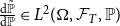
(ii) The Radon–Nikodym derivative
$\frac {\mathop {}\!\mathrm{d} \tilde {\mathbb{P}}}{\mathop {}\!\mathrm{d} \mathbb{P}} \in L^{2}(\Omega , \mathcal{F}_{T}, \mathbb{P})$
, where
$L^{2}(\Omega , \mathcal{F}_{T},\mathbb{P})$
is the space of square-integrable,
$\mathcal{F}_T$
-measurable, random variables on
$(\Omega , \mathbb{P})$
. -
(iii) The surplus process
$\{ R_t \}_{t \in \mathcal{T}}$
is an
$(\mathbb{F}, \tilde {\mathbb{P}})$
-martingale. In particular,
for any
\begin{equation*} \tilde {\mathbb{E}}\left [ R_{t}\mid \mathcal{F}_{s}\right ] = R_{s}, \tilde {\mathbb{P}}-\textit {a.s}. \end{equation*}
$0\leq s\leq t\leq T$
, where
$\tilde {\mathbb{E}} [\cdot \,|\, \mathcal{F}_s ]$
denotes the conditional expectation given
$\mathcal{F}_s$
with respect to
$\tilde {\mathbb{P}}$
.




To simplify the discussion, given that we assume a constant interest rate, we take the interest rate to be zero. The framework extends straightforwardly to a non-zero constant interest rate by working with discounted surplus processes, as detailed in Appendix A. However, the incorporation of a stochastic interest rate, while it is more realistic, would complicate the modeling framework. Consequently, to simplify the discussion, we do not consider the situation of a stochastic interest rate here.
Remark 1. It may be noted that Definition 5 (iii) can be expressed as follows: assuming $R_{0}=0$
, (i.e., the surplus at the initial time
$R_{0}=0$
, (i.e., the surplus at the initial time $0$
is zero), we have:
$0$
is zero), we have:
 \begin{equation*} \tilde {\mathbb{E}}\!\left (R_{t}\mid \mathcal{F}_{0}\right ) = \tilde {\mathbb{E}}\!\left (P_{t}-C_{t}\mid \mathcal{F}_{0}\right ) = \tilde {\mathbb{E}}\!\left (P_{t}\mid \mathcal{F}_{0}\right ) - \tilde {\mathbb{E}}\!\left (C_{t}\mid \mathcal{F}_{0}\right ) = 0. \end{equation*}
Consequently,
 \begin{equation*} \tilde {\mathbb{E}}\!\left (C_{t}\mid \mathcal{F}_{0}\right ) = \tilde {\mathbb{E}}\!\left (P_{t}\mid \mathcal{F}_{0}\right ) = \text{an arbitrage-free insurance premium.} \end{equation*}
In the sequel, we shall adopt the Esscher transform to select an equivalent martingale measure. To do this, we start with Theorem 1, giving a (local) martingale, which will be considered when specifying the Radon–Nikodym derivative for changing probability measures via the Esscher transform.
Theorem 1.
Suppose that $\rho \gt 0$
for all
$\rho \gt 0$
for all $t \in \mathcal{T}$
. For constants
$t \in \mathcal{T}$
. For constants $\theta , \nu , \phi , {\psi }$
, we have an
$\theta , \nu , \phi , {\psi }$
, we have an $(\mathbb{F}, \mathbb{P})$
-(local)-martingale
$(\mathbb{F}, \mathbb{P})$
-(local)-martingale
 \begin{equation*} \mathrm{e}^{K(t)} \theta ^{N_t} \mathrm{e}^{ B(t) \lambda _t} \, \mathrm{e}^{-\nu C_t} {\mathrm{e}^{\phi \Lambda _t} \psi ^{M_t}}, \quad t \in \mathcal{T}, \end{equation*}
if $\{B(t),K(t)\}_{t \in \mathcal{T}}$
satisfy the non-linear ordinary differential equations (ODE):
$\{B(t),K(t)\}_{t \in \mathcal{T}}$
satisfy the non-linear ordinary differential equations (ODE):
 \begin{align*} B^{\prime }(t) - \delta B(t) + \theta \, {\hat {j}(\nu )} \, \hat {g}(\!-\!B(t)) \, + {\phi } -1 &= 0,\\ K^{\prime }(t) + a \delta B(t) + \rho \left [{\psi } \hat {h}(\!-\!B(t)) - 1 \right ] &= 0, \end{align*}
where ${\hat h} (\! \cdot \!)$
,
${\hat h} (\! \cdot \!)$
, ${\hat g} (\! \cdot \!)$
and
${\hat g} (\! \cdot \!)$
and ${\hat j} (\! \cdot \!)$
are the Laplace transforms defined by Eq. (
2.3
).
${\hat j} (\! \cdot \!)$
are the Laplace transforms defined by Eq. (
2.3
).
Proof.
Firstly, we consider a function $f( \lambda _{t},N_{t},C_{t}, {M_t}, {\Lambda _t}, t)$
defined by:
$f( \lambda _{t},N_{t},C_{t}, {M_t}, {\Lambda _t}, t)$
defined by:
 \begin{equation*} f( \lambda _{t},N_{t},C_{t}, {M_t}, {\Lambda _t}, t) \,=\, \mathrm{e}^{K(t)} \theta ^{N_t} \mathrm{e}^{ B(t) \lambda _t} \, \mathrm{e}^{-\nu C_t} {\mathrm{e}^{\phi \Lambda _t} \psi ^{M_t}}, \end{equation*}
for constants $\theta ,{\psi },\nu$
.
$\theta ,{\psi },\nu$
.
Applying Itô’s differentiation rule to $f$
gives:
$f$
gives:
 \begin{eqnarray*} f (\lambda _t, N_t, C_t, M_t, \Lambda _t, t) &=& f (\lambda _0, N_0, C_0, M_0, \Lambda _0, 0) + \int ^{t}_{0} \delta (a - \lambda _u) \frac {\partial f}{\partial \lambda } \mathop {}\!\mathrm{d} u + \int ^{t}_{0} \lambda _u \frac {\partial f}{\partial \Lambda } \mathop {}\!\mathrm{d} u \\ && + \int ^{t}_{0} \lambda _{u-} \bigg ( \int ^{\infty }_{0} \int ^{\infty }_{0} f (\lambda _{u-} + y, N_{u-} + 1, C_{u-} + \xi , M_{u-}, \Lambda _{u-}, u) \\ && \quad \times \mathop {}\!\mathrm{d} G(y) \mathop {}\!\mathrm{d} J (\xi ) - f (\lambda _{u-}, N_{u-}, C_{u-}, M_{u-}, \Lambda _{u-}, u) \bigg ) \mathop {}\!\mathrm{d} u \\ && + \int ^{t}_{0} \rho _{u-} \bigg ( \int ^{\infty }_{0} f (\lambda _{u-} + x, N_{u-}, C_{u-}, M_{u-} + 1, \Lambda _{u-}, u) \mathop {}\!\mathrm{d} H (x) \\ && \quad - f(\lambda _{u-}, N_{u-}, C_{u-}, M_{u-}, \Lambda _{u-}, u) \bigg ) \mathop {}\!\mathrm{d} u + \mathcal{M}_t, \end{eqnarray*}
where $\{ \mathcal{M}_t \}_{t \ge 0}$
is an
$\{ \mathcal{M}_t \}_{t \ge 0}$
is an $(\mathbb{F}, \mathbb{P})$
-(local)-martingale.
$(\mathbb{F}, \mathbb{P})$
-(local)-martingale.
Using Eq. (2.2), we have:
 \begin{align*} &\hspace {-0.5cm} f (\lambda _t, N_t, C_t, M_t, \Lambda _t, t) \\ &= f (\lambda _0, N_0, C_0, M_0, \Lambda _0, 0) + \int ^{t}_{0} \mathcal{A} f (\lambda _{u-}, N_{u-}, C_{u-}, M_{u-}, \Lambda _{u-}, u) \mathop {}\!\mathrm{d} u + \mathcal{M}_t. \end{align*}
If $\mathcal{A} f( \lambda , n,c,{m}, {\Lambda }, t)=0$
then
$\mathcal{A} f( \lambda , n,c,{m}, {\Lambda }, t)=0$
then
 \begin{equation*} f (\lambda _t, N_t, C_t, M_t, \Lambda _t, t) = f (\lambda _0, N_0, C_0, M_0, \Lambda _0, 0) + \mathcal{M}_t, \end{equation*}
i.e., $\{ f (\lambda _t, N_t, C_t, M_t, \Lambda _t, t) \}_{t \in \mathcal{T}}$
is an
$\{ f (\lambda _t, N_t, C_t, M_t, \Lambda _t, t) \}_{t \in \mathcal{T}}$
is an $(\mathbb{F}, \mathbb{P})$
-(local)-martingale.
$(\mathbb{F}, \mathbb{P})$
-(local)-martingale.
Plug $f(\lambda _t, N_t, C_t, M_t, \Lambda _t, t)$
into the generator in Eq. (2.2) for the standard DCP and set
$f(\lambda _t, N_t, C_t, M_t, \Lambda _t, t)$
into the generator in Eq. (2.2) for the standard DCP and set $\mathcal{A} f( \lambda , n,c,{m}, {\Lambda }, t)=0$
, where
$\mathcal{A} f( \lambda , n,c,{m}, {\Lambda }, t)=0$
, where
 \begin{equation*} f( \lambda , n,c,{m}, {\Lambda }, t) = \mathrm{e}^{K(t)} \theta ^{n} \mathrm{e}^{ B(t) \lambda } \, \mathrm{e}^{-\nu c} {\mathrm{e}^{\phi \Lambda } \psi ^{m}} , \end{equation*}
i.e.,
 \begin{align*} 0&= K^{\prime }(t) + B^{\prime }(t) \lambda +\delta \left ( a- \lambda \right ) B(t) + \lambda \phi \\ &\quad + \lambda \left [ \theta \int _{0}^{\infty }\int _{0}^{\infty } \mathrm{e}^{ B(t) y} \mathrm{e}^{-\nu \xi } \mathop {}\!\mathrm{d} G(y)\mathop {}\!\mathrm{d} J(\xi )-1 \right ] + \rho \left [ \psi \int _{0}^{\infty } \mathrm{e}^{ B(t) x} \mathop {}\!\mathrm{d} H(x)- 1 \right ], \\ 0 &= \lambda \left \{ B^{\prime }(t) - \delta B(t) + \phi + \theta \int _{0}^{\infty }\int _{0}^{\infty } \mathrm{e}^{ B(t) y} \mathrm{e}^{-\nu \xi } \mathop {}\!\mathrm{d} G(y)\mathop {}\!\mathrm{d} J(\xi )-1 \right \} \\ &\quad + K^{\prime }(t) + \delta a B(t) + \rho \left [ \psi \int _{0}^{\infty } \mathrm{e}^{ B(t) x} \mathop {}\!\mathrm{d} H(x)- 1 \right ] \\ 0 &= \lambda \bigg \{ B^{\prime }(t) - \delta B(t) + \phi + \theta \hat {j}(\nu ) \hat {g}(\!-\!B(t)) -1 \bigg \} + K^{\prime }(t) + \delta a B(t) + \rho \left [ \psi \hat {h}(\!-\!B(t))- 1 \right ], \end{align*}
where
 \begin{equation*} \hat {j}(\nu ) \, :\!= \, \int _{0}^{\infty } \mathrm{e}^{-\nu \xi } \mathop {}\!\mathrm{d} J(\xi ), \qquad \hat {g}(B(t)) \, :\!= \, \int _{0}^{\infty } \mathrm{e}^{ -B(t) y} \mathop {}\!\mathrm{d} G(y), \qquad {\hat {h}}(B(t)) \, :\!= \, \int _{0}^{\infty } \mathrm{e}^{- B(t) x} \mathop {}\!\mathrm{d} {H}(x). \end{equation*}
So, we have the ODEs for $B(t),K(t)$
,
$B(t),K(t)$
,
 \begin{align*} B^{\prime }(t) - \delta B(t) + \theta \, {\hat {j}(\nu )} \, \hat {g}(\!-\!B(t)) \, + {\phi } -1 &= 0,\\ K^{\prime }(t) + a \delta B(t) + \rho \left [{\psi } \hat {h}(\!-\!B(t)) - 1 \right ] &= 0. \end{align*}
Hence, the theorem is proved.
The following theorem provides the existence and uniqueness results for the solutions to the nonlinear ODEs in Theorem 1.
Theorem 2. Assume that the following conditions hold:
 \begin{equation*} \theta ,\psi \geq 1, \quad \nu \lt 0 \quad (\hat {j}(\nu )\gt 1), \qquad \phi = -(\theta \, \hat {j}(\nu ) -1) \lt 0, \qquad \delta \gt \theta \, \hat {j}(\nu ) \mu _G. \end{equation*}
Then the following statements hold:
-
1. There exists a unique solution for
$B(t)$
to the nonlinear ODE in Theorem
1
with the initial condition
$B(0)=b\gt 0$
and the stationary condition
$\delta \gt \mu _G$
such that
where
\begin{equation*} B(t)\ =\ \mathcal{G}^{-1}(t), \qquad t \geq 0, \end{equation*}
\begin{equation*} \mathcal{G}(B) \, :\!= \, \int ^{B}_b \frac {\mathop {}\!\mathrm{d} u }{f_1( u )}, \qquad B\in (b, B^+ ), \end{equation*}
and
\begin{equation*} f_1 (B) \, :\!= \, \delta B -\theta \, \hat {j}(\nu ) \, ( \hat {g}(\!-\!B ) -1 ). \end{equation*}
$B^+\gt 0$
is the smallest positive solution to
$f_1 (B)=0$
.
-
2. Then, there exists a unique solution for
$K(t)$
to the nonlinear ODE in Theorem
1
with the boundary condition
$K(0) = 0$
such that
\begin{equation*} K (t) = -a \delta \int _0^t B(s)\mathop {}\!\mathrm{d} s + \rho \int _0^t \big [ 1 - {\psi } \hat {h}(-B(s)) \big ] \mathop {}\!\mathrm{d} s. \end{equation*}


Proof. Assume that
 \begin{equation*} \theta ,\psi \geq 1, \quad \nu \lt 0 \quad (\hat {\,j}(\nu )\gt 1), \qquad \phi = -(\theta \, \hat {j}(\nu ) -1) \lt 0, \qquad \delta \gt \theta \, \hat {j}(\nu ) \mu _G. \end{equation*}
Then the nonlinear ODE in Theorem 1 can be written as:
 \begin{equation} \frac {\mathop {}\!\mathrm{d} B(t)}{\mathop {}\!\mathrm{d} t} = \delta B - \theta \, \hat {j}(\nu ) \, \left ( \hat {g}(\!-\!B ) -1 \right ), \end{equation}
with the initial condition $B(0)=b\gt 0$
and the stationary condition
$B(0)=b\gt 0$
and the stationary condition $\delta \gt \mu _G$
. Define
$\delta \gt \mu _G$
. Define
 \begin{equation} f_1(B) \, :\!= \, \delta B -\theta \, \hat {j}(\nu ) \, \left ( \hat {g}(\!-\!B ) -1 \right )\!. \end{equation}
Then
 \begin{equation} f_1(0)= 0. \end{equation}
Also,
 \begin{equation} \left . \frac {\mathop {}\!\mathrm{d} f_1 (B)}{\mathop {}\!\mathrm{d} B} \right |_{B=0} =\ \delta - \theta \hat {j} (\nu ) \mu _G\ \gt \ 0. \end{equation}
Taking the second-order derivative of $f_1 (B)$
with respect to
$f_1 (B)$
with respect to $B$
gives:
$B$
gives:
 \begin{equation*} \frac {\mathop {}\!\mathrm{d}^2 f_1 (B) }{\mathop {}\!\mathrm{d} B^2} = - \theta \hat {j} (\nu ) \int ^{\infty }_{0} {y^2 \mathrm{e}^{B y} \mathop {}\!\mathrm{d} G(y)} \lt 0. \end{equation*}
Then $f_1 (B)$
is strictly concave. This, together with Eqs. (3.4) and (3.5), imply that
$f_1 (B)$
is strictly concave. This, together with Eqs. (3.4) and (3.5), imply that $f_1(B) \gt 0$
, for
$f_1(B) \gt 0$
, for $B\in \left (0, B^+\right )$
, where
$B\in \left (0, B^+\right )$
, where $B^+\gt 0$
is the smallest positive solution to
$B^+\gt 0$
is the smallest positive solution to $f_1 (B)=0$
.
$f_1 (B)=0$
.
Taking $B = u$
and
$B = u$
and $t = \tau$
, Eqs. (3.2) and (3.3) lead to:
$t = \tau$
, Eqs. (3.2) and (3.3) lead to:
 \begin{equation} \frac {\mathop {}\!\mathrm{d} u}{f_1 (u)} = \mathop {}\!\mathrm{d} \tau , \quad u \in (0, B^+). \end{equation}
Recall that $B (0) = b$
and
$B (0) = b$
and $B (t) = B$
. Then integrating both sides of Eq. (3.6) gives:
$B (t) = B$
. Then integrating both sides of Eq. (3.6) gives:
 \begin{equation} \int ^{B}_{b} \frac {\mathop {}\!\mathrm{d} u}{f_1 (u)} = \int ^{t}_{0} \mathop {}\!\mathrm{d} \tau = t, \quad B \in (0, B^+). \end{equation}
Define the left-hand side of Eq. (3.7) as:
 \begin{equation} \mathcal{G}(B) \, :\!= \, \int ^{B}_b \frac {\mathop {}\!\mathrm{d} u}{f_1( u )}, \qquad B\in \left (b, B^+ \right )\!. \end{equation}
Note that $\mathcal{G}(B)$
is a continuous and strictly increasing function for
$\mathcal{G}(B)$
is a continuous and strictly increasing function for $B \in (b, B^+)$
. Consequently, its inverse
$B \in (b, B^+)$
. Consequently, its inverse $\mathcal{G}^{-1}$
exists and is uniquely determined. The function
$\mathcal{G}^{-1}$
exists and is uniquely determined. The function $\mathcal{G} \, : \, (b, B^+) \to (0, \infty )$
is defined in Eq. (3.8) is an isomorphism. The inverse
$\mathcal{G} \, : \, (b, B^+) \to (0, \infty )$
is defined in Eq. (3.8) is an isomorphism. The inverse $\mathcal{G}^{-1} (t)$
then gives the solution
$\mathcal{G}^{-1} (t)$
then gives the solution $B(t) = B$
to the nonlinear ODE in Theorem 1 with the initial condition
$B(t) = B$
to the nonlinear ODE in Theorem 1 with the initial condition $B (0) = b \gt 0$
as follows:
$B (0) = b \gt 0$
as follows:
 \begin{equation*} B(t) \,\,=\,\, \mathcal{G}^{-1}(t) \,\, \in \,\, (b, B^+), \qquad t \gt 0. \end{equation*}
Once $B(t)$
is uniquely determined as above,
$B(t)$
is uniquely determined as above, $K(t)$
can be obtained from the second nonlinear ODE in Theorem 1 with the boundary condition
$K(t)$
can be obtained from the second nonlinear ODE in Theorem 1 with the boundary condition $K(0) = 0$
simply as
$K(0) = 0$
simply as
 \begin{equation*} K (t) = -a \delta \int _0^t B(s)\mathop {}\!\mathrm{d} s + \rho \int _0^t \left [ 1 - {\psi } \hat {h}(\!-\!B(s)) \right ] \mathop {}\!\mathrm{d} s. \end{equation*}
Recall that $\{\mathrm{e}^{K(t)} \theta ^{N_t} \mathrm{e}^{ B(t) \lambda _t} \, \mathrm{e}^{-\nu C_t} {\mathrm{e}^{\phi \Lambda _t} \psi ^{M_t}} \}_{t \in \mathcal{T}}$
is a (local)-martingale. We suppose that some (suitable) square integrability conditions hold so that
$\{\mathrm{e}^{K(t)} \theta ^{N_t} \mathrm{e}^{ B(t) \lambda _t} \, \mathrm{e}^{-\nu C_t} {\mathrm{e}^{\phi \Lambda _t} \psi ^{M_t}} \}_{t \in \mathcal{T}}$
is a (local)-martingale. We suppose that some (suitable) square integrability conditions hold so that $\{\mathrm{e}^{K(t)} \theta ^{N_t} \mathrm{e}^{ B(t) \lambda _t} \, \mathrm{e}^{-\nu C_t} {\mathrm{e}^{\phi \Lambda _t} \psi ^{M_t}} \}_{t \in \mathcal{T}}$
is a square-integrable martingale. We now describe how the probability laws of
$\{\mathrm{e}^{K(t)} \theta ^{N_t} \mathrm{e}^{ B(t) \lambda _t} \, \mathrm{e}^{-\nu C_t} {\mathrm{e}^{\phi \Lambda _t} \psi ^{M_t}} \}_{t \in \mathcal{T}}$
is a square-integrable martingale. We now describe how the probability laws of $N_{t}$
and
$N_{t}$
and $C_t$
change after changing the probability measures by the Esscher transform. Firstly, from Theorem 1,
$C_t$
change after changing the probability measures by the Esscher transform. Firstly, from Theorem 1, $\{ \mathrm{e}^{K(t)} \theta ^{N_t} \mathrm{e}^{ B(t) \lambda _t} \, \mathrm{e}^{-\nu C_t} {\mathrm{e}^{\phi \Lambda _t} \psi ^{M_t}} \}_{t \in \mathcal{T}}$
is an
$\{ \mathrm{e}^{K(t)} \theta ^{N_t} \mathrm{e}^{ B(t) \lambda _t} \, \mathrm{e}^{-\nu C_t} {\mathrm{e}^{\phi \Lambda _t} \psi ^{M_t}} \}_{t \in \mathcal{T}}$
is an $(\mathbb{F}, \mathbb{P})$
-martingale. Then, for all
$(\mathbb{F}, \mathbb{P})$
-martingale. Then, for all $t \in \mathcal{T}$
,
$t \in \mathcal{T}$
,
 \begin{equation*} \mathbb{E}_0 [\mathrm{e}^{K(t)} \theta ^{N_t} \mathrm{e}^{ B(t) \lambda _t} \, \mathrm{e}^{-\nu C_t} {\mathrm{e}^{\phi \Lambda _t} \psi ^{M_t}} ] = \mathrm{e}^{K(0)} \theta ^{N_0} \mathrm{e}^{ B(0) \lambda _0} \, \mathrm{e}^{-\nu C_0} {\mathrm{e}^{\phi \Lambda _0} \psi ^{M_0}}. \end{equation*}
Consider the following (normalized) $\mathbb{F}$
-adapted process
$\mathbb{F}$
-adapted process $\{\zeta _t \}_{t \in \mathcal{T}}$
:
$\{\zeta _t \}_{t \in \mathcal{T}}$
:
 \begin{equation} \zeta _t \, :\!= \, \frac { \mathrm{e}^{K(t)} \theta ^{N_t} \mathrm{e}^{ B(t) \lambda _t} \, \mathrm{e}^{-\nu C_t} {\mathrm{e}^{\phi \Lambda _t} \psi ^{M_t}} }{\mathbb{E}_0 [\mathrm{e}^{K(t)} \theta ^{N_t} \mathrm{e}^{ B(t) \lambda _t} \, \mathrm{e}^{-\nu C_t} {\mathrm{e}^{\phi \Lambda _t} \psi ^{M_t}} ]} = \frac {\mathrm{e}^{K(t)} \theta ^{N_t} \mathrm{e}^{ B(t) \lambda _t} \, \mathrm{e}^{-\nu C_t} {\mathrm{e}^{\phi \Lambda _t} \psi ^{M_t}} }{\mathrm{e}^{K(0)} \theta ^{N_0} \mathrm{e}^{ B(0) \lambda _0} \, \mathrm{e}^{-\nu C_0} {\mathrm{e}^{\phi \Lambda _0} \psi ^{M_0}}}. \end{equation}
It is clear that by its definition in Eq. (3.9) and Theorem 1, $\{ \zeta _t \}_{t \in \mathcal{T}}$
is an
$\{ \zeta _t \}_{t \in \mathcal{T}}$
is an $(\mathbb{F}, \mathbb{P})$
-martingale. For each
$(\mathbb{F}, \mathbb{P})$
-martingale. For each $t \in \mathcal{T}$
,
$t \in \mathcal{T}$
, $\zeta _t \gt 0$
,
$\zeta _t \gt 0$
, $\mathbb{P}$
-a.s. Furthermore,
$\mathbb{P}$
-a.s. Furthermore, $\mathbb{E}_0 [\zeta _t] = \zeta _0 = 1$
. Consequently, a new probability measure
$\mathbb{E}_0 [\zeta _t] = \zeta _0 = 1$
. Consequently, a new probability measure $\tilde {\mathbb{P}}$
, which is equivalent to the original probability measure
$\tilde {\mathbb{P}}$
, which is equivalent to the original probability measure $\mathbb{P}$
on
$\mathbb{P}$
on $\mathcal{F}_T$
, can be defined by putting:
$\mathcal{F}_T$
, can be defined by putting:
 \begin{equation*} \frac {d \tilde {\mathbb{P}}}{d \mathbb{P}} \bigg |_{\mathcal{F}_T} \, :\!= \, \zeta _T. \end{equation*}
Given that $\{ \zeta _t \}_{t \in \mathcal{T}}$
is a square-integrable
$\{ \zeta _t \}_{t \in \mathcal{T}}$
is a square-integrable $(\mathbb{F}, \mathbb{P})$
–martingale, then
$(\mathbb{F}, \mathbb{P})$
–martingale, then
 \begin{eqnarray*} \mathbb{E} \left [ \bigg | \frac {d \tilde {\mathbb{P}}}{d \mathbb{P}} \bigg |^2 \right ] = \mathbb{E} [ | \zeta _T |^2] \lt \infty . \end{eqnarray*}
Consequently, Definition 5 (ii) is satisfied.
We refer to related works employing the exponential change of measure: Palmowski and Rolski (Reference Palmowski and Rolski2002) for Markov processes, Kallsen and Shiryaev (Reference Kallsen and Shiryaev2002) via the cumulant process and Esscher transform, and Palmowski et al. (Reference Palmowski, Pojer and Thonhauser2025) for ruin probabilities with Hawkes arrivals.
3.2 Infinitesimal generator under the equivalent martingale measure
Let $\tilde {\mathcal{A}}$
denote the infinitesimal generator of the joint process
$\tilde {\mathcal{A}}$
denote the infinitesimal generator of the joint process $\{ ( \lambda _{t},N_{t},C_{t}, M_t, \Lambda _t, t) \}_{t \in \mathcal{T}}$
under the new probability measure
$\{ ( \lambda _{t},N_{t},C_{t}, M_t, \Lambda _t, t) \}_{t \in \mathcal{T}}$
under the new probability measure $\tilde {\mathbb{P}}$
. The key to study how the probability laws of
$\tilde {\mathbb{P}}$
. The key to study how the probability laws of $N_{t}$
and
$N_{t}$
and $C_t$
change after changing probability measures by the Esscher transform is to obtain the infinitesimal generator
$C_t$
change after changing probability measures by the Esscher transform is to obtain the infinitesimal generator $\tilde {\mathcal{A}}$
. This is to be achieved in Theorem 3 and Corollary 1 to be presented in the sequel. To do so, we start with a technical lemma.
$\tilde {\mathcal{A}}$
. This is to be achieved in Theorem 3 and Corollary 1 to be presented in the sequel. To do so, we start with a technical lemma.
Lemma 1.
Assume that $\tilde {f}( \lambda , n,c,{m}, {\Lambda }, t) = \tilde {f}( \lambda , t)$
for all
$\tilde {f}( \lambda , n,c,{m}, {\Lambda }, t) = \tilde {f}( \lambda , t)$
for all $n$
,
$n$
, $c$
,
$c$
, $m$
, and
$m$
, and $\Lambda$
, and that
$\Lambda$
, and that $\mathrm{e}^{-B(t)\lambda _t}$
is a martingale. Consider
$\mathrm{e}^{-B(t)\lambda _t}$
is a martingale. Consider $B(t)\gt 0$
for some
$B(t)\gt 0$
for some $t \gt 0$
. Then
$t \gt 0$
. Then
 \begin{align} \tilde {\mathcal{A}} \tilde {f} (\lambda , 0) = \frac { \mathcal{A} \bigl (\, \tilde {f}(\lambda , 0)\, \mathrm{e}^{{-}B(t)\lambda _t}\bigr ) } { \mathrm{e}^{-B(t)\lambda _t} }. \\[-23pt] \nonumber \end{align}
Proof.
The generator of the process $(\lambda _t, t)$
acting on a function
$(\lambda _t, t)$
acting on a function $\tilde {f}(\lambda , t)$
with respect to the equivalent martingale probability measure is
$\tilde {f}(\lambda , t)$
with respect to the equivalent martingale probability measure is
 \begin{equation} \tilde {\mathcal{A}} \tilde {f} (\lambda , 0) = \lim _{t \downarrow 0} \frac {\tilde {\mathbb{E}}\!\left [\tilde {f}(\lambda _t, t) \mid \lambda _0 = \lambda \right ] - \tilde {f}(\lambda , 0)}{t}. \end{equation}
We will use
 \begin{equation*} \frac {\mathrm{e}^{-B(t)\lambda _t}}{\mathbb{E}\!\left (\mathrm{e}^{-B(t)\lambda _t}\right )} \end{equation*}
as the Radon–Nikodym derivative to define the equivalent martingale probability measure, where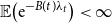 $\mathbb{E}\!\left (\mathrm{e}^{-B(t)\lambda _t}\right ) \lt \infty$
. Hence, the expected value of
$\mathbb{E}\!\left (\mathrm{e}^{-B(t)\lambda _t}\right ) \lt \infty$
. Hence, the expected value of $\tilde {f}(\lambda _t, t)$
given
$\tilde {f}(\lambda _t, t)$
given $\lambda$
with respect to the equivalent martingale probability measure is
$\lambda$
with respect to the equivalent martingale probability measure is
 \begin{equation} \tilde {\mathbb{E}}\!\left [\tilde {f}(\lambda _t, t) \mid \lambda _0 = \lambda \right ] = \frac {\mathbb{E}\!\left [\tilde {f}(\lambda _t, t)\, \mathrm{e}^{-B(t)\lambda _t} \mid \lambda _0 = \lambda \right ]} {\mathbb{E}\!\left (\mathrm{e}^{-B(t)\lambda _t} \mid \lambda _0 = \lambda \right )}. \end{equation}
Since the denominator in (3.12) is a martingale, it becomes
 \begin{equation} \tilde {\mathbb{E}}\!\left [\tilde {f}(\lambda _t, t) \mid \lambda _0 = \lambda \right ] = \frac {\tilde {f}(\lambda , 0)\, \mathrm{e}^{-B(t)\lambda } + \int _0^t \mathbb{E}\!\left [ \mathcal{A} \tilde {f}(\lambda _s, s)\, \mathrm{e}^{-B(t)\lambda _s} \mid \lambda _0 = \lambda \right ] \mathop {}\!\mathrm{d} s} {\mathrm{e}^{-B(t)\lambda }}. \end{equation}
Substituting (3.13) into (3.11) gives
 \begin{equation} \tilde {\mathcal{A}} \tilde {f}(\lambda , 0) = \frac {1}{\mathrm{e}^{-B(t)\lambda }} \lim _{t \downarrow 0} \frac {1}{t} \int _0^t \mathbb{E}\!\left [ \mathcal{A} \tilde {f}(\lambda _s, s)\, \mathrm{e}^{-B(t)\lambda _s} \mid \lambda _0 = \lambda \right ] \mathop {}\!\mathrm{d} s. \end{equation}
Therefore, by Dynkin’s formula (see Øksendal, Reference Øksendal2013), (3.10) follows immediately.
Theorem 3. Suppose that the following conditions hold:
 \begin{equation*} \theta ,\psi \geq 1, \quad \nu \lt 0 \quad (\hat {j}(\nu )\gt 1), \qquad \phi = -(\theta \, \hat {j}(\nu ) -1) \lt 0, \qquad \delta \gt \theta \, \hat {j}(\nu ) \mu _G. \end{equation*}
Write, for all $t \in \mathcal{T}$
,
$t \in \mathcal{T}$
,
 \begin{align*} \mathop {}\!\mathrm{d} \tilde {G}(y; \, t) &\, :\!= \, \frac {\mathrm{e}^{B(t) y}}{\hat {g}(\!-\!B(t))} \mathop {}\!\mathrm{d} G(y), & \mathop {}\!\mathrm{d} {\tilde {H}}(x; \, t) &\, :\!= \, \frac {\mathrm{e}^{ B(t) x}}{\hat {h}(\!-\!B(t))} \mathop {}\!\mathrm{d} {H}(x), \\ \mathop {}\!\mathrm{d} \tilde {J}(\xi ) &\, :\!= \, \frac {\mathrm{e}^{-\nu \xi }}{\hat {j}(\nu )} \mathop {}\!\mathrm{d} J(\xi ), & \tilde {\rho }(t) &\, :\!= \, \psi \hat {h}(\!-\!B(t))\, \rho . \end{align*}
Let $\mathcal{D} (\mathcal{A})$
and
$\mathcal{D} (\mathcal{A})$
and $\mathcal{D} (\tilde {\mathcal{A}})$
denote the domains of the infinitesimal generators
$\mathcal{D} (\tilde {\mathcal{A}})$
denote the domains of the infinitesimal generators $\mathcal{A}$
and
$\mathcal{A}$
and $\tilde {\mathcal{A}}$
, respectively. Then, for any function
$\tilde {\mathcal{A}}$
, respectively. Then, for any function $\tilde {f} \in \mathcal{D} (\mathcal{A}) \cap \mathcal{D} (\tilde {\mathcal{A}})$
,
$\tilde {f} \in \mathcal{D} (\mathcal{A}) \cap \mathcal{D} (\tilde {\mathcal{A}})$
,
 \begin{align} &\hspace {-0.5cm}\tilde {\mathcal{A}} \tilde {f}( \lambda , n,c,{m}, {\Lambda }, t) \notag \\ &= \frac {\partial \tilde {f}}{\partial t} + \lambda \frac {\partial \tilde {f}}{\partial \Lambda } + \delta \left ( a-\lambda \right )\frac {\partial \tilde {f}}{\partial \lambda } \notag \\ &\quad + \theta \hat {j}(\nu ) \hat {g}(\!-\!B(t))\, \lambda \left [ \int _{0}^{\infty }\int _{0}^{\infty } \tilde {f}(\lambda +y,n+1,c+\xi ,{m},{\Lambda },t) \mathop {}\!\mathrm{d} \tilde {G}(y; \, t) \mathop {}\!\mathrm{d} \tilde {J}(\xi ) - \tilde {f} \right ] \notag \\ &\quad + \tilde {\rho }(t) \left [ \int _{0}^{\infty }\tilde {f}( \lambda +x,n,c,{m+1},{\Lambda },t) \mathop {}\!\mathrm{d} \tilde {H}(x; \, t) - \tilde {f} \right ]. \end{align}
Proof. Set
 \begin{equation*} \mathrm{e}^{K(t)} \theta ^{n} \mathrm{e}^{ B(t) \lambda } \, \mathrm{e}^{-\nu c} {\mathrm{e}^{\phi \Lambda } \psi ^{m}} \tilde {f}( \lambda , n,c,{m}, {\Lambda }, t), \end{equation*}
into the generator in Eq. (2.2) and from Lemma 1, we have
 \begin{align*} &\hspace {-0.1cm} \tilde {\mathcal{A}} \tilde {f}( \lambda , n,c,{m}, {\Lambda }, t) \\ &= \frac { \mathcal{A} \bigg \{ \mathrm{e}^{K(t)} \theta ^{n} \mathrm{e}^{ B(t) \lambda } \, \mathrm{e}^{-\nu c} {\mathrm{e}^{\phi \Lambda } \psi ^{m}} \tilde {f}( \lambda , n,c,{m}, {\Lambda }, t) \bigg \} }{\mathrm{e}^{K(t)} \theta ^{n} \mathrm{e}^{ B(t) \lambda } \, \mathrm{e}^{-\nu c} {\mathrm{e}^{\phi \Lambda } \psi ^{m}}} + + \\ &= \frac {\partial \tilde {f}}{\partial t} + \bigg ( K^{\prime }(t) + B^{\prime }(t) \lambda \bigg ) \tilde {f} + \delta \left ( a-\lambda \right ) \left ( \frac {\partial \tilde {f}}{\partial \lambda } + B(t) \tilde {f} \right ) + {\lambda \left ( \frac {\partial \tilde {f}}{\partial \Lambda } + \phi \tilde {f} \right )} \\ &\quad + \lambda \left [ \theta \hat {j}(\nu ) \hat {g}(\!-\!B(t)) \int _{0}^{\infty }\int _{0}^{\infty } \tilde {f}(\lambda +y,n+1,c+\xi ,{m},{\Lambda },t) \frac {\mathrm{e}^{ B(t) y}}{\hat {g}(\!-\!B(t))} \mathop {}\!\mathrm{d} G(y) \frac {\mathrm{e}^{-\nu \xi }}{\hat {j}(\nu )} \mathop {}\!\mathrm{d} J(\xi ) -\tilde {f} \right ] \\ &\quad +\rho \left [ \psi \hat {h}(\!-\!B(t)) \int _{0}^{\infty }\tilde {f}( \lambda +x,n,c,{m+1},{\Lambda },t) \frac {\mathrm{e}^{ B(t) x}}{\hat {h}(\!-\!B(t))} \mathop {}\!\mathrm{d} H(x) - \tilde {f} \right ]\!. \end{align*}
Define
 \begin{equation*} \mathop {}\!\mathrm{d} \tilde {G}(y; \, t)\, :\!= \, \frac {\mathrm{e}^{ B(t) y}}{\hat {g}(\!-\!B(t))} \mathop {}\!\mathrm{d} G(y), \qquad \mathop {}\!\mathrm{d} {\tilde {H}}(x; \, t) \, :\!= \, \frac {\mathrm{e}^{ B(t) x}}{\hat {h}(\!-\!B(t))} \mathop {}\!\mathrm{d} {H}(x), \qquad \mathop {}\!\mathrm{d} \tilde {J}(\xi ) \, :\!= \, \frac {\mathrm{e}^{-\nu \xi }}{\hat {j}(\nu )} \mathop {}\!\mathrm{d} J(\xi ), \end{equation*}
then,
 \begin{align*} &\hspace {-0.1cm} \tilde {\mathcal{A}} \tilde {f}( \lambda , n,c,{m}, {\Lambda }, t) \\ &= \frac {\partial \tilde {f}}{\partial t} + \bigg ( K^{\prime }(t) + B^{\prime }(t) \lambda \bigg ) \tilde {f} + \delta \left ( a-\lambda \right ) \left ( \frac {\partial \tilde {f}}{\partial \lambda } + B(t) \tilde {f} \right ) + {\lambda \left ( \frac {\partial \tilde {f}}{\partial \Lambda } + \phi \tilde {f} \right )} \\ &\quad + \lambda \left [ \theta \hat {j}(\nu ) \hat {g}(\!-\!B(t)) \int _{0}^{\infty }\int _{0}^{\infty } \tilde {f}(\lambda +y,n+1,c+\xi ,{m},{\Lambda },t) \mathop {}\!\mathrm{d} \tilde {G}(y; \, t) \mathop {}\!\mathrm{d} \tilde {J}(\xi ) -\tilde {f} \right ] \\ &\quad +\rho \left [ \psi \hat {h}(\!-\!B(t)) \int _{0}^{\infty }\tilde {f}( \lambda +x,n,c,{m+1},{\Lambda },t) \mathop {}\!\mathrm{d} \tilde {H}(x; \, t) - \tilde {f} \right ] \\ &= \bigg [ K^{\prime }(t) + a \delta B(t) + \bigg ( B^{\prime }(t) - \delta B(t) +\phi \bigg ) \lambda \bigg] \,\tilde {f} + \frac {\partial \tilde {f}}{\partial t} + \lambda \frac {\partial \tilde {f}}{\partial \Lambda } + \delta \left ( a-\lambda \right )\frac {\partial \tilde {f}}{\partial \lambda } \\ &\quad + \lambda \left [ \theta \hat {j}(\nu ) \hat {g}(\!-\!B(t)) \int _{0}^{\infty }\int _{0}^{\infty } \tilde {f}(\lambda +y,n+1,c+\xi ,{m},{\Lambda },t) \mathop {}\!\mathrm{d} \tilde {G}(y; \, t) \mathop {}\!\mathrm{d} \tilde {J}(\xi ) -\tilde {f} \right ] \\ &\quad +\rho \left [ \psi \hat {h}(\!-\!B(t)) \int _{0}^{\infty }\tilde {f}( \lambda +x,n,c,{m+1},{\Lambda },t) \mathop {}\!\mathrm{d} \tilde {H}(x; \, t) - \tilde {f} \right ] \\ &= \frac {\partial \tilde {f}}{\partial t} + \lambda \frac {\partial \tilde {f}}{\partial \Lambda } + \delta \left ( a-\lambda \right )\frac {\partial \tilde {f}}{\partial \lambda } \\ &\quad + \theta \hat {j}(\nu ) \hat {g}(\!-\!B(t)) \lambda \left [ \int _{0}^{\infty }\int _{0}^{\infty } \tilde {f}(\lambda +y,n+1,c+\xi ,{m},{\Lambda },t) \mathop {}\!\mathrm{d} \tilde {G}(y; \, t) \mathop {}\!\mathrm{d} \tilde {J}(\xi ) - \tilde {f} \right ] \\ &\quad +\psi \hat {h}(\!-\!B(t)) \,\rho \left [ \int _{0}^{\infty }\tilde {f}( \lambda +x,n,c,{m+1},{\Lambda },t) \mathop {}\!\mathrm{d} \tilde {H}(x; \, t) - \tilde {f} \right ]\!. \end{align*}
Define
 \begin{equation*} \tilde {\rho }(t)\, :\!= \,\psi \hat {h}(\!-\!B(t))\, \rho , \end{equation*}
and consequently, Eq. (3.15) is obtained.
Theorem 3 yields the following:
-
(i) The intensity process
$\lambda _t$
has changed to
$\tilde {\lambda }_t \, :\!= \, \theta \hat {j}(\nu )\hat {g}(\!-\!B(t))\,\lambda _t$
, which is time-dependent; -
(ii) The self-exciting jump size measure
$\mathop {}\!\mathrm{d} G(y)$
has changed to
$\mathop {}\!\mathrm{d} \tilde {G}(y; \, t)\, :\!= \, \frac {\mathrm{e}^{ B(t) y}}{\hat {g}(\!-\!B(t))} \mathop {}\!\mathrm{d} G(y)$
, which now depends on time; -
(iii) The rate of external-exciting jump arrival
$\rho$
has changed to
$\tilde {\rho }(t)\, :\!= \,\psi \hat {h}(\!-\!B(t))\, \rho$
, which now depends on time; -
(iv) The external-exciting jump size measure
$\mathop {}\!\mathrm{d} H(x)$
has changed to
$\mathop {}\!\mathrm{d} {\tilde {H}}(x; \, t) \, :\!= \, \frac {\mathrm{e}^{ B(t) x}}{\hat {h}(\!-\!B(t))} \mathop {}\!\mathrm{d} {H}(x)$
, which now depends on time; -
(v) The claim/loss size measure
$\mathop {}\!\mathrm{d} J\left ( \xi \right )$
has changed to
$\mathop {}\!\mathrm{d} \tilde {J}(\xi ) \, :\!= \, \frac {\mathrm{e}^{-\nu \xi }}{\hat {j}(\nu )} \mathop {}\!\mathrm{d} J(\xi )$
.









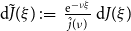
The Esscher transform provides a transparent and actuarially consistent mechanism for risk-adjusted pricing of catastrophe reinsurance. Under the transformed probability measure based on the Esscher transformation, the arrival intensity $\lambda _t$
, jump size measures
$\lambda _t$
, jump size measures $\tilde {G}(\! \cdot; \, t)$
,
$\tilde {G}(\! \cdot; \, t)$
, $\tilde {H}(\! \cdot; \, t)$
,
$\tilde {H}(\! \cdot; \, t)$
, $\tilde {J}(\! \cdot \!)$
, and external excitation factor
$\tilde {J}(\! \cdot \!)$
, and external excitation factor $\tilde {\rho }(t)$
are adjusted to reflect aversion to extreme losses and catastrophic risk, jointly determining an arbitrage-free premium consistent with actuarial principles. In particular, (i) scaling of the intensity process represents a frequency loading; (ii) tilted self-exciting jump sizes place greater weights on contagion-driven shocks; (iii) time-dependent adjustment of external-exciting arrivals loads for systemic shocks; (iv) transformed external-exciting jump sizes increase the likelihood of large external shocks; and (v) the Esscher tilting on claim sizes acts as a severity-based loading. Together, these adjustments allow reinsurers to incorporate risk aversion in a granular and interpretable manner, distinguishing between frequency, contagion, external shocks, and severity risks, while preserving a consistent arbitrage-free valuation framework.
$\tilde {\rho }(t)$
are adjusted to reflect aversion to extreme losses and catastrophic risk, jointly determining an arbitrage-free premium consistent with actuarial principles. In particular, (i) scaling of the intensity process represents a frequency loading; (ii) tilted self-exciting jump sizes place greater weights on contagion-driven shocks; (iii) time-dependent adjustment of external-exciting arrivals loads for systemic shocks; (iv) transformed external-exciting jump sizes increase the likelihood of large external shocks; and (v) the Esscher tilting on claim sizes acts as a severity-based loading. Together, these adjustments allow reinsurers to incorporate risk aversion in a granular and interpretable manner, distinguishing between frequency, contagion, external shocks, and severity risks, while preserving a consistent arbitrage-free valuation framework.
The result in Theorem 3 can be rewritten by defining
 \begin{equation*} \tilde {\lambda }_t \, :\!= \, \theta \hat {j}(\nu ) \hat {g}(\!-\!B(t)) \lambda _t, \qquad \tilde {\Lambda }_t \, :\!= \, \theta \hat {j}(\nu ) \hat {g}(\!-\!B(t)) \Lambda _t, \end{equation*}
for any time $t \in \mathcal{T}$
, which is presented in Corollary 1 below.
$t \in \mathcal{T}$
, which is presented in Corollary 1 below.
Corollary 1. The generator in Eq. (3.15) can be alternatively expressed by
 \begin{align} &\hspace {-0.5cm} \tilde {\mathcal{A}} \tilde {f}( \tilde {\lambda }, n,c,{m}, {\tilde {\Lambda }}, t) \notag \\ &= \frac {\partial \tilde {f}}{\partial t} + \tilde {\lambda } \frac {\partial \tilde {f}}{\partial \tilde {\Lambda } } + \delta \bigg ( \theta \hat {j}(\nu ) \hat {g}(\!-\!B(t)) \, a - \tilde {\lambda } \bigg )\frac {\partial \tilde {f}}{\partial \tilde {\lambda } } \notag \\ &\quad + \tilde {\lambda } \left [ \int _{0}^{\infty }\int _{0}^{\infty } \tilde {f}(\tilde {\lambda } +u,n+1,c+\xi ,{m},{\tilde {\Lambda }},t) \mathop {}\!\mathrm{d} \tilde {G}\left ( \frac {u}{\theta \hat {j}(\nu ) \hat {g}(\!-\!B(t))} ; t \right ) \mathop {}\!\mathrm{d} \tilde {J}(\xi ) - \tilde {f} \right ] \notag \\ &\quad + \tilde {\rho }(t) \left [ \int _{0}^{\infty }\tilde {f}( \tilde {\lambda } + v,n,c,{m+1},{\tilde {\Lambda }},t) \mathop {}\!\mathrm{d} \tilde {H}\left ( \frac {v}{\theta \hat {j}(\nu ) \hat {g}(\!-\!B(t))} ; t\right ) - \tilde {f} \right ]. \end{align}
Proof. Define
 \begin{equation*} \tilde {\lambda } \, :\!= \, \theta \hat {j}(\nu ) \hat {g}(\!-\!B(t)) \lambda , \qquad \tilde {\Lambda } \, :\!= \, \theta \hat {j}(\nu ) \hat {g}(\!-\!B(t)) \Lambda , \end{equation*}
and we have
 \begin{align*} &\hspace {-0.5cm}\tilde {\mathcal{A}} \tilde {f}( \tilde {\lambda }, n,c,{m}, {\tilde {\Lambda }}, t) \\ &= \frac {\partial \tilde {f}}{\partial t} + \tilde {\lambda } \frac {\partial \tilde {f}}{\partial \tilde {\Lambda } } + \delta \bigg ( \theta \hat {j}(\nu ) \hat {g}(\!-\!B(t)) \, a - \tilde {\lambda } \bigg )\frac {\partial \tilde {f}}{\partial \tilde {\lambda } } \\ &\quad + \tilde {\lambda } \left [ \int _{0}^{\infty }\int _{0}^{\infty } \tilde {f}(\tilde {\lambda } +\theta \hat {j}(\nu ) \hat {g}(\!-\!B(t)) y,n+1,c+\xi ,{m},{\tilde {\Lambda }},t) \mathop {}\!\mathrm{d} \tilde {G}(y; \, t) \mathop {}\!\mathrm{d} \tilde {J}(\xi ) - \tilde {f} \right ] \\ &\quad + \tilde {\rho }(t) \left [ \int _{0}^{\infty }\tilde {f}( \tilde {\lambda } + \theta \hat {j}(\nu ) \hat {g}(\!-\!B(t)) x,n,c,{m+1},{\tilde {\Lambda }},t) \mathop {}\!\mathrm{d} \tilde {H}(x; \, t) - \tilde {f} \right ]\!. \end{align*}
Changing variables $u=\theta \hat {j}(\nu ) \hat {g}(\!-\!B(t)) y, v=\theta \hat {j}(\nu ) \hat {g}(\!-\!B(t)) x$
, we have Eq. (3.16).
$u=\theta \hat {j}(\nu ) \hat {g}(\!-\!B(t)) y, v=\theta \hat {j}(\nu ) \hat {g}(\!-\!B(t)) x$
, we have Eq. (3.16).
Corollary 2. More explicitly, for
 \begin{equation*} \mathop {}\!\mathrm{d} \tilde {G}(y; \, t) = \tilde {g}(y; \, t) \mathop {}\!\mathrm{d} y, \qquad \mathop {}\!\mathrm{d} {\tilde {H}}(x; \, t) = {\tilde {h}}(x; \, t) \mathop {}\!\mathrm{d} x, \end{equation*}
we have the transforms
 \begin{align*} a \ &\rightarrow \ \theta \hat {j}(\nu ) \hat {g}(\!-\!{B(t)}) \, a; \\ \rho \ &\rightarrow \ \psi \hat {h}(\!-\!{B(t)})\, \rho ;\\ h(v) \ &\rightarrow \ \frac {\tilde {h}\left ( \frac {v}{\theta \hat {j}(\nu ) \hat {g}(\!-\!{B(t)})}; \, t \right )}{\theta \hat {j}(\nu ) \hat {g}(\!-\!{B(t)})} ; \\ g(u) \ &\rightarrow \ \frac { \tilde {g}\left ( \frac {u}{\theta \hat {j}(\nu ) \hat {g}(\!-\!{B(t)})}; \, t\right ) }{\theta \hat {j}(\nu ) \hat {g}(\!-\!{B(t)})} ; \\ j(\xi ) \ &\rightarrow \ \tilde {j}(\xi ) , \end{align*}
where
 \begin{equation*} \tilde {g}(y; \, t) \, :\!= \, \frac {\mathrm{e}^{B(t) y}}{\hat {g}(\!-\!B(t))} g (y), \qquad \tilde {h}(x; \, t) \, :\!= \, \frac {\mathrm{e}^{B(t) x}}{\hat {h}(\!-\!B(t))} h(x), \qquad \tilde {j}(\xi ) \, :\!= \, \frac {\mathrm{e}^{-\nu \xi }}{\hat {j}(\nu )} j (\xi ). \end{equation*}
Proof. Based on Corollary 1, in particular for
 \begin{equation*} \mathop {}\!\mathrm{d} \tilde {G}(y; \, t) = \tilde {g}(y; \, t) \mathop {}\!\mathrm{d} y, \qquad \mathop {}\!\mathrm{d} {\tilde {H}}(x; \, t) = {\tilde {h}}(x; \, t) \mathop {}\!\mathrm{d} x, \end{equation*}
we have
 \begin{align*} &\hspace {-0.5cm}\tilde {\mathcal{A}} \tilde {f}( \tilde {\lambda }, n,c,{m}, {\tilde {\Lambda }}, t) \\ &= \frac {\partial \tilde {f}}{\partial t} + \tilde {\lambda } \frac {\partial \tilde {f}}{\partial \tilde {\Lambda } } + \delta \bigg ( \theta \hat {j}(\nu ) \hat {g}(\!-\!B(t)) \, a - \tilde {\lambda } \bigg )\frac {\partial \tilde {f}}{\partial \tilde {\lambda } } \\ &\quad + \tilde {\lambda } \left [ \int _{0}^{\infty }\int _{0}^{\infty } \tilde {f}(\tilde {\lambda } +u,n+1,c+\xi ,{m},{\tilde {\Lambda }},t) \mathop {}\!\mathrm{d} \tilde {J}(\xi ) \, \frac { \tilde {g}( \frac {u}{\theta \hat {j}(\nu ) \hat {g}(\!-\!B(t))}\, ;t) }{\theta \hat {j}(\nu ) \hat {g}(\!-\!B(t))} \mathop {}\!\mathrm{d} u - \tilde {f} \right ] \\ &\quad + \tilde {\rho }(t) \left [ \int _{0}^{\infty }\tilde {f}( \tilde {\lambda } + v,n,c,{m+1},{\tilde {\Lambda }},t) \frac {\tilde {h}( \frac {v}{\theta \hat {j}(\nu ) \hat {g}(\!-\!B(t))} ;t )}{\theta \hat {j}(\nu ) \hat {g}(\!-\!B(t))} \mathop {}\!\mathrm{d} v - \tilde {f} \right ]\!. \end{align*}
Then, we have the transforms.
Note that the parameters of a CDCP under the original measure $\mathbb{P}$
are all constants, whereas the parameters of a CDCP under the new measure
$\mathbb{P}$
are all constants, whereas the parameters of a CDCP under the new measure $\tilde {\mathbb{P}}$
become time-varying (except for the intensity-decay rate
$\tilde {\mathbb{P}}$
become time-varying (except for the intensity-decay rate $\delta$
), i.e., a time-inhomogeneous CDCP.
$\delta$
), i.e., a time-inhomogeneous CDCP.
In reality, a “hard” market in a (re)insurance industry occurs when the supply of coverage available is lower than its demand. This leads to a higher (re)insurance premium, reduced (or stopped) coverage, and less competition among (re)insurance providers. The Southern California wildfires of January 2025 further exacerbated this, as rising losses from catastrophic events, coupled with the increasing costs of reinsurance and construction, have prompted insurers like State Farm to limit or withdraw coverage in high-risk areas, intensifying the strain on the market.
There are several reasons why a hardening reinsurance market prevails. Firstly, there has been increasing frequency and severity of losses attributed to catastrophic events due to El Niño and La Niña. Secondly, a high inflation regime has been in force, which may be partly due to turbulence in macroeconomic conditions. Thirdly, there has been a growing number of emerging events such as cyber and pandemic events.
In a hardening reinsurance market, it may be reasonable for a reinsurer to calculate the premium of a catastrophe reinsurance contract in a more conservative and prudent way. To illustrate this situation in our current modeling setup, certain assumptions are imposed on $\theta ,{\psi }, \nu , B(t)$
such that there would be more external-exciting jump arrivals in a given period of time, a higher value of self-exciting intensity, higher values of their jump sizes, as well as a larger size of claim or loss. To take on these additional risks in the hardening market, a reinsurer requires higher compensation. Furthermore, it may be reasonable to postulate that the reinsurer aims to maximize their shareholders’ wealth via earning profits. To this end, the reinsurer may charge a higher premium than the “break-even” premium. The latter is given by the expected claims evaluated under the original (real-world) probability measure. In the hardening market,
$\theta ,{\psi }, \nu , B(t)$
such that there would be more external-exciting jump arrivals in a given period of time, a higher value of self-exciting intensity, higher values of their jump sizes, as well as a larger size of claim or loss. To take on these additional risks in the hardening market, a reinsurer requires higher compensation. Furthermore, it may be reasonable to postulate that the reinsurer aims to maximize their shareholders’ wealth via earning profits. To this end, the reinsurer may charge a higher premium than the “break-even” premium. The latter is given by the expected claims evaluated under the original (real-world) probability measure. In the hardening market, $\theta ,{\psi }, \nu , B(t)$
may be thought of as security loading factors by which positive gross premium should be finally charged. In fact, based on Corollary 2, if the gross premium is always positive, we shall have the conditions
$\theta ,{\psi }, \nu , B(t)$
may be thought of as security loading factors by which positive gross premium should be finally charged. In fact, based on Corollary 2, if the gross premium is always positive, we shall have the conditions
 \begin{equation*} \theta ,{\psi }\geq 1, \qquad \nu \lt 0, \qquad {\mbox{$B(t)\gt 0$ for some $t \gt 0$}}. \end{equation*}
From an economic perspective, the Esscher parameters $(\theta ,\psi ,\nu )$
provide a parsimonious representation of reinsurer risk preferences under hard market conditions. In particular, the transformed intensity process
$(\theta ,\psi ,\nu )$
provide a parsimonious representation of reinsurer risk preferences under hard market conditions. In particular, the transformed intensity process
 \begin{equation*} \tilde {\lambda }_t \, :\!= \, \theta \hat {j}(\nu )\hat {g}(\!-\!B(t))\,\lambda _t \end{equation*}
introduces a time-dependent loading on claim arrivals, reflecting heightened sensitivity to both claim frequency and loss severity during periods of elevated risk. The parameter $\theta$
acts as a frequency loading on the baseline arrival intensity, while the factor
$\theta$
acts as a frequency loading on the baseline arrival intensity, while the factor $\hat {j}(\nu )\hat {g}(\!-\!B(t))$
captures the interaction between severity aversion and contagion-driven dynamics. Similarly, the parameter
$\hat {j}(\nu )\hat {g}(\!-\!B(t))$
captures the interaction between severity aversion and contagion-driven dynamics. Similarly, the parameter $\psi$
scales the arrival rate of externally driven shocks, representing increased concern about systemic events. The Esscher parameter
$\psi$
scales the arrival rate of externally driven shocks, representing increased concern about systemic events. The Esscher parameter $\nu \lt 0$
induces a severity-based loading by tilting the claim size distribution toward larger losses, thereby increasing the contribution of catastrophic events to the premium.
$\nu \lt 0$
induces a severity-based loading by tilting the claim size distribution toward larger losses, thereby increasing the contribution of catastrophic events to the premium.
In a hard reinsurance market, these choices of the parameters are consistent with observed outcomes such as higher premiums and tighter underwriting, resulting in a conservative valuation. On the other hand, reinsurers may also limit coverage in high-risk regions by transferring part of the risk whenever alternative capacity is available. In this sense, the Esscher parameters $(\theta ,\psi ,\nu )$
may serve as reduced-form measures incorporating market risk aversion and capital scarcity into catastrophe reinsurance pricing.
$(\theta ,\psi ,\nu )$
may serve as reduced-form measures incorporating market risk aversion and capital scarcity into catastrophe reinsurance pricing.
3.3 Special case: exponential/gamma distributions for jump sizes
Before closing this section, we show the explicit transformation for the computation of arbitrage-free catastrophe stop-loss reinsurance premiums in Section 4.
Corollary 3 (Special case: exponential/gamma distributions for jump sizes). In particular, we assume that external-exciting and self-exciting jump sizes in the intensity process follow exponential distributions $H \sim \mathsf{Exp}(\alpha ), G \sim \mathsf{Exp}(\beta )$
, respectively, i.e.,
$H \sim \mathsf{Exp}(\alpha ), G \sim \mathsf{Exp}(\beta )$
, respectively, i.e.,
 \begin{equation*} h(x) =\alpha \mathrm{e}^{-\alpha x}, \qquad g(y) =\beta \mathrm{e}^{-\beta y},\ \qquad \alpha ,\beta \gt 0, \end{equation*}
and claim/loss sizes follow the gamma distribution $J \sim \mathsf{Gamma}(\gamma ,\eta )$
with the rate parameter
$J \sim \mathsf{Gamma}(\gamma ,\eta )$
with the rate parameter $\gamma$
and shape parameter
$\gamma$
and shape parameter $\eta$
, i.e.,
$\eta$
, i.e.,
 \begin{equation*} j\left ( \xi \right ) = \frac {\gamma ^{\eta }\xi ^{\eta -1}\mathrm{e}^{-\gamma \xi }}{\left ( \eta -1\right ) !}, \qquad \gamma \gt 0, \eta \geq 1. \end{equation*}
Then, we have the transforms
 \begin{align*} a \ &\rightarrow \ \theta \Bigl (1 + \frac {\nu }{\gamma }\Bigr )^{-\eta } \frac {\beta }{\beta - B(t)} a; \\ \rho \ &\rightarrow \ \psi \frac {\alpha }{\alpha - B(t) } \, \rho ;\\ J \sim \mathsf{Gamma}(\gamma ,\eta )\ &\rightarrow \ \mathsf{Gamma}(\gamma +\nu , \eta ); \\ H \sim \mathsf{Exp}(\alpha ) \ &\rightarrow \ \mathsf{Exp}(\lambda _h); \\ G \sim \mathsf{Exp}(\beta ) \ &\rightarrow \ \mathsf{Exp}(\lambda _g); \end{align*}
where
 \begin{equation*} \lambda _h \, :\!= \, \frac {\alpha - B(t)}{\theta \left (1 + \frac {\nu }{\gamma }\right )^{-\eta } \frac {\beta }{\beta -B(t)}}, \qquad \lambda _g \, :\!= \, \frac {\beta - B(t)}{\theta \left (1 + \frac {\nu }{\gamma }\right )^{-\eta } \frac {\beta }{\beta -B(t)}}, \qquad \nu \in (\!-{\gamma} ,0). \end{equation*}
Proof.
In particular for exponential distributions, $H \sim \mathsf{Exp}(\alpha ), G \sim \mathsf{Exp}(\beta )$
, i.e.,
$H \sim \mathsf{Exp}(\alpha ), G \sim \mathsf{Exp}(\beta )$
, i.e.,
 \begin{equation*} h(x) =\alpha \mathrm{e}^{-\alpha x}, \qquad g(y) =\beta \mathrm{e}^{-\beta y}, \qquad \alpha ,\beta \gt 0, \end{equation*}
we have
 \begin{equation*} \hat {g}(\!-\!B(t)) = \frac {\beta }{\beta -B(t)}, \qquad \hat {h}(\!-\!B(t)) = \frac {\alpha }{\alpha -B(t)}, \end{equation*}
 \begin{equation*} \tilde {g}(y) = (\beta -B(t)) \mathrm{e}^{-(\beta -B(t)) y}, \qquad \tilde {h}(x) = (\alpha -B(t)) \mathrm{e}^{-(\alpha -B(t)) x}. \end{equation*}
Similarly, for gamma distribution $J \sim \mathsf{Gamma}(\gamma ,\eta )$
, we have the transform to
$J \sim \mathsf{Gamma}(\gamma ,\eta )$
, we have the transform to $\mathsf{Gamma}({\gamma +\nu ,\eta })$
, since
$\mathsf{Gamma}({\gamma +\nu ,\eta })$
, since
 \begin{align*} j\left ( \xi \right ) &= \frac {\gamma ^{\eta }\xi ^{\eta -1}\mathrm{e}^{-\gamma \xi }}{\left ( \eta -1\right ) !}, \qquad \gamma \gt 0, \eta \geq 1, \qquad \hat {j}(\nu ) = \left (\frac {\gamma }{\gamma + \nu } \right )^{\eta }, \\ \tilde {j}(\xi ) &= \frac {\mathrm{e}^{-\nu \xi }}{\hat {j}(\nu )} j (\xi ) \,\,=\,\, \frac {\mathrm{e}^{-\nu \xi }}{\hat {j}(\nu )} \frac {\gamma ^{\eta }\xi ^{\eta -1}\mathrm{e}^{-\gamma \xi }}{\left ( \eta -1\right ) !} \,\,=\,\, \frac { (\gamma + \nu )^{\eta } \xi ^{\eta -1} \mathrm{e}^{-(\gamma +\nu ) \xi } }{\left ( \eta -1\right ) !}. \end{align*}
Finally, we obtain the results by applying the transforms in Corollary 2.
In fact, the original distributional structure of the underlying risk process via this change of measure is preserved. We may also need the stationary condition for a CDCP under the new measure, i.e.,
 \begin{equation*} \delta \,\,\gt \,\, \frac {1}{\lambda _g} \,\,=\,\, \theta \left ( \frac {\gamma }{\gamma +\nu }\right )^{\eta } \frac {\beta }{(\beta - B(t))^2}, \end{equation*}
where $\delta$
and
$\delta$
and $\frac {1}{\lambda _g}$
are the decay rate and the mean of exponentially distributed self-excited jump sizes under the new measure for a CDCP, respectively, according to Corollary 3. So, for implementations, we have to set the decay rate
$\frac {1}{\lambda _g}$
are the decay rate and the mean of exponentially distributed self-excited jump sizes under the new measure for a CDCP, respectively, according to Corollary 3. So, for implementations, we have to set the decay rate $\delta$
relatively large together with the condition
$\delta$
relatively large together with the condition $\delta \gt \theta \, \hat {j}(\nu ) \mu _G =\theta \, \hat {j}(\nu ) \frac {1}{\beta }$
required in Theorem 2 for the existence and uniqueness of the solutions of the ODEs to hold. This constraint on
$\delta \gt \theta \, \hat {j}(\nu ) \mu _G =\theta \, \hat {j}(\nu ) \frac {1}{\beta }$
required in Theorem 2 for the existence and uniqueness of the solutions of the ODEs to hold. This constraint on $\delta$
is required in our model. In other words, the model may not be applicable if this constraint on
$\delta$
is required in our model. In other words, the model may not be applicable if this constraint on $\delta$
does not hold. This may represent a limitation of the model.
$\delta$
does not hold. This may represent a limitation of the model.
Note that, for the ODE of $B(t)$
, we have
$B(t)$
, we have
 \begin{equation*} f_1 (B) = \delta B \left ( \frac {B - \left ( \beta - \frac {1}{\delta } \theta \, \hat {j}(\nu ) \right ) }{B-\beta } \right)\!, \end{equation*}
where $B^+\, :\!= \,\beta - \frac {1}{\delta } \theta \, \hat {j}(\nu ) \gt 0$
or
$B^+\, :\!= \,\beta - \frac {1}{\delta } \theta \, \hat {j}(\nu ) \gt 0$
or $\delta \beta \gt \theta \, \hat {j}(\nu )$
. Define
$\delta \beta \gt \theta \, \hat {j}(\nu )$
. Define
 \begin{equation} \mathcal{G}(B) \, :\!= \, \int ^{B}_b \frac {\mathop {}\!\mathrm{d} u}{f_1(u)}, \qquad B\in \left (b, B^+ \right )\!. \end{equation}
Note that $\mathcal{G}(B)$
is a strictly increasing function and
$\mathcal{G}(B)$
is a strictly increasing function and
 \begin{equation*} \lim _{B \downarrow b}\mathcal{G}(B) = 0, \qquad \lim _{B \uparrow B^+ }\mathcal{G}(B) = \infty . \end{equation*}
We have its inverse as the solution to $B(t)$
as
$B(t)$
as
 \begin{equation*} B(t) \ = \ \mathcal{G}^{-1}(t), \qquad t \geq 0. \end{equation*}
Finally, we have the following three types of parameter settings:
-
1. If
$\alpha \geq B^+$
, then
$B(t) \in (0, \alpha )$
for any time
$t \geq 0$
; -
2. If
$\alpha \in (b,B^+)$
, then
$B(t) \in (0, \alpha )$
for
$t \in [0, t^* )$
, where
$t^* \, :\!= \,\mathcal{G}(\alpha ) \gt 0$
from Eq. (3.17); -
3. If
$\alpha \in (0,b]$
, then
$B(t) \in (0, \alpha )$
; there is no solution for
$B(t) \in (0, \alpha ),t\geq 0$
;






where $b\gt 0,{B^+=\beta - \frac {1}{\delta } \theta \, {\hat {j}}(\nu ) \gt 0}$
. Note that the function
$b\gt 0,{B^+=\beta - \frac {1}{\delta } \theta \, {\hat {j}}(\nu ) \gt 0}$
. Note that the function $\mathcal{G}(\! \cdot \!)$
in Eq. (3.17) shall be derived fully analytically. However, its inverse
$\mathcal{G}(\! \cdot \!)$
in Eq. (3.17) shall be derived fully analytically. However, its inverse $\mathcal{G}^{-1}(\! \cdot \!)$
has to be solved numerically.
$\mathcal{G}^{-1}(\! \cdot \!)$
has to be solved numerically.
The first type of parameter setting (i.e., $\alpha \geq B^+$
) is the most ideal. For numerical examples, it is suggested that
$\alpha \geq B^+$
) is the most ideal. For numerical examples, it is suggested that $b$
is chosen to be small and close to zero, and
$b$
is chosen to be small and close to zero, and $\alpha$
is relatively large.
$\alpha$
is relatively large.
In particular, if $\beta \rightarrow \infty$
, then all self-exciting jump sizes approach to zero, which degenerates to the pure shot-noise intensity model of Dassios and Jang (Reference Dassios and Jang2003).
$\beta \rightarrow \infty$
, then all self-exciting jump sizes approach to zero, which degenerates to the pure shot-noise intensity model of Dassios and Jang (Reference Dassios and Jang2003).
Corollary 4 (Expectations for exponential/gamma distributions). When $H \sim \mathsf{Exp}(\alpha )$
,
$H \sim \mathsf{Exp}(\alpha )$
, $G \sim \mathsf{Exp}(\beta )$
, and
$G \sim \mathsf{Exp}(\beta )$
, and $J \sim \mathsf{Gamma}(\gamma ,\eta )$
, the expectations are as follows:
$J \sim \mathsf{Gamma}(\gamma ,\eta )$
, the expectations are as follows:
 \begin{equation*} \begin{aligned} \tilde {\mathbb{E}}[ \lambda _t \mid \lambda _0]\ &= \ \lambda _0 \mathrm{e}^{-\int _0^t I(s) \mathop {}\!\mathrm{d} s} + \mathrm{e}^{-\int _0^t I(s) \mathop {}\!\mathrm{d} s} \theta \left ( \frac {\gamma }{\gamma +\nu }\right ) ^{\eta } \\ &\quad \times \int _0^t \mathrm{e}^{\int _0^s I(u) \mathop {}\!\mathrm{d} u} \left ( \frac {\beta }{\beta -B(s)}\right ) \left \{ \psi \alpha \rho \left ( \frac {1}{\alpha -B(s)}\right )^{2} + a \delta \right \} \mathop {}\!\mathrm{d} s. \end{aligned} \end{equation*}
 \begin{equation*} \tilde {\mathbb{E}}[ N_t \mid \lambda _0 ] = \int _{0}^{t} \tilde {\mathbb{E}}[ \lambda _{s} \mid \lambda _{0} ] \mathop {}\!\mathrm{d} s \end{equation*}
 \begin{equation*} \tilde {\mathbb{E}}[ C_t \mid \lambda _0 ] = \mu _{\widetilde {J}} \int _0^t \tilde {\mathbb{E}}[ \lambda _s \mid \lambda _0 ] \mathop {}\!\mathrm{d} s \end{equation*}
where $ I(s) = \delta - \left [\theta \left ( \frac {\gamma }{\gamma +\nu }\right )^{\eta } \left ( \frac {\beta }{\beta -B(s) }\right ) \right ]/[\beta -B(s)]$
and
$ I(s) = \delta - \left [\theta \left ( \frac {\gamma }{\gamma +\nu }\right )^{\eta } \left ( \frac {\beta }{\beta -B(s) }\right ) \right ]/[\beta -B(s)]$
and $\mu _{\widetilde {J}} = \eta /(\gamma + \nu )$
.
$\mu _{\widetilde {J}} = \eta /(\gamma + \nu )$
.
Proof. These follow from substituting the transformed values into Proposition 2.
For illustrative purposes, we have used a Gamma distribution for claim sizes, which yields a closed-form expression under the Esscher transform, $\tilde {J} \sim \mathsf{Gamma}(\gamma +\nu ,\eta )$
. The Gamma family is a standard choice in actuarial modeling of claim severities (Bühlmann, Reference Bühlmann1970, Page 7) and offers analytical tractability that facilitates clear interpretation of the pricing mechanism. While heavier-tailed alternatives, such as the Pareto distribution,
$\tilde {J} \sim \mathsf{Gamma}(\gamma +\nu ,\eta )$
. The Gamma family is a standard choice in actuarial modeling of claim severities (Bühlmann, Reference Bühlmann1970, Page 7) and offers analytical tractability that facilitates clear interpretation of the pricing mechanism. While heavier-tailed alternatives, such as the Pareto distribution,
 \begin{equation*} j(\xi ) = \frac {\Gamma (\omega + k)\, \zeta ^\omega \, \xi ^{k-1}} {\Gamma (\omega )\, \Gamma (k)\, (\zeta + \xi )^{\omega + k}}, \qquad \omega \gt 0,\ \zeta \gt 0,\ k\gt 0, \end{equation*}
are commonly employed to model large insurance losses (Albrecher et al., Reference Albrecher, Beirlant and Teugels2017, Chapters 3–4), their form is not preserved under the Esscher transform and instead acquires an exponential tilt. Nevertheless, the corresponding Laplace transform $\hat {j}(\nu )$
exists under suitable parameter conditions and can be evaluated numerically. Heavier-tailed claim size distributions typically lead to higher premium levels, reflecting increased tail risk. In this sense, the Gamma specification, including the exponential distribution as a special case, serves as a benchmark for assessing the impact of tail heaviness on catastrophe reinsurance pricing. The results presented here therefore illustrate the qualitative behavior of the model, while extensions to Pareto or other heavy-tailed distributions may be explored in future work via numerical sensitivity analysis.
$\hat {j}(\nu )$
exists under suitable parameter conditions and can be evaluated numerically. Heavier-tailed claim size distributions typically lead to higher premium levels, reflecting increased tail risk. In this sense, the Gamma specification, including the exponential distribution as a special case, serves as a benchmark for assessing the impact of tail heaviness on catastrophe reinsurance pricing. The results presented here therefore illustrate the qualitative behavior of the model, while extensions to Pareto or other heavy-tailed distributions may be explored in future work via numerical sensitivity analysis.
4. Numerical results
In this section, we provide arbitrage-free catastrophe stop-loss reinsurance premiums via the Monte Carlo simulation method. We also examine the sensitivity analyses for the retention level, the Esscher parameters, and the intensity parameters.
4.1 Pricing of a stop-loss reinsurance contract
The total loss excess over $L$
, which is a retention limit, up to time
$L$
, which is a retention limit, up to time $t$
is
$t$
is $(C_{t}-L)^+$
. Then the stop-loss reinsurance gross premium at time 0 (i.e., under
$(C_{t}-L)^+$
. Then the stop-loss reinsurance gross premium at time 0 (i.e., under $\tilde {\mathbb{P}}$
) is
$\tilde {\mathbb{P}}$
) is
 \begin{equation} \tilde {\mathbb{E}}[(C_t - L)^+]. \end{equation}
Its Monte Carlo estimate will be denoted by $\widehat {\tilde {\mathbb{E}}}[(C_t - L)^+]$
, and the corresponding estimate under
$\widehat {\tilde {\mathbb{E}}}[(C_t - L)^+]$
, and the corresponding estimate under $\mathbb{P}$
will be denoted by
$\mathbb{P}$
will be denoted by $\widehat {\mathbb{E}}[(C_t - L)^+]$
. For this section, we consider
$\widehat {\mathbb{E}}[(C_t - L)^+]$
. For this section, we consider
 \begin{equation*} \alpha = 2, \beta = 1, \eta = 3, \gamma = 0.4 , \end{equation*}
 \begin{equation*} \delta = 3, \rho = 4, a = 1, \lambda _0 = 1, t = 1 , \end{equation*}
 \begin{equation*} \nu = -0.05, \theta = 1.25, \psi = 1.25, \phi = - (\theta \hat {j}(\nu ) - 1). \end{equation*}
The parameter values adopted in the numerical examples are chosen for illustrative purposes. They are used to demonstrate the qualitative behavior of the model, as well as the impacts of contagion and risk loading on reinsurance premiums, rather than to provide an empirical calibration to a specific portfolio. Similar parameter ranges are commonly adopted in the dynamic contagion and self-exciting point process literature to study clustering effects and catastrophic risk (Dassios and Zhao (Reference Dassios and Zhao2011); Jang and Oh (Reference Jang and Oh2021, Reference Jang and Oh2025)).
In practice, model parameters may be estimated from historical catastrophe or large-loss data using standard inference techniques for point processes with latent or stochastic intensities, including likelihood-based methods, moment-based estimators, and filtering approaches. General statistical frameworks for point process inference are discussed in Karr (Reference Karr1991) and Daley and Vere-Jones (Reference Daley and Vere-Jones2008), while modern likelihood-based methodologies for self-exciting and Hawkes-type processes are presented in Laub et al. (Reference Laub, Lee and Taimre2022). Related filtering approaches in insurance risk models are studied in Dassios and Jang (Reference Dassios and Jang2005) for shot-noise Cox processes, and similar ideas may be adapted to the dynamic contagion setting considered here.
While maximum likelihood estimators for point process parameters and some of their statistical properties have been studied, the estimation of shot-noise Cox processes, and in particular the analysis of their asymptotic properties, has received comparatively less attention. These challenges are further compounded when time-varying parameters are present, suggesting promising opportunities for future research, particularly in the context of dynamic contagion models for insurance risk.
For each combination of parameters, $10^5$
crude Monte Carlo (CMC) samples of
$10^5$
crude Monte Carlo (CMC) samples of $C_t$
under
$C_t$
under $\tilde {\mathbb{P}}$
have been used to estimate Eq. (4.1) in Table 1. The corresponding values under
$\tilde {\mathbb{P}}$
have been used to estimate Eq. (4.1) in Table 1. The corresponding values under $\mathbb{P}$
are also provided in the same table.
$\mathbb{P}$
are also provided in the same table.
The stop-loss CMC estimates $\widehat {\mathbb{E}}[(C_t - L)^+]$
under the original measure and
$\widehat {\mathbb{E}}[(C_t - L)^+]$
under the original measure and $\widehat {\tilde {\mathbb{E}}}[(C_t - L)^+]$
under the Esscher measure for different
$\widehat {\tilde {\mathbb{E}}}[(C_t - L)^+]$
under the Esscher measure for different $L$
retention levels
$L$
retention levels
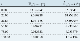
A collection of 25 sample paths of $C_t$
and the corresponding
$C_t$
and the corresponding $\lambda _t$
for the compound dynamic contagion process under the original measure
$\lambda _t$
for the compound dynamic contagion process under the original measure $\mathbb{P}$
(left column) and the tilted measure
$\mathbb{P}$
(left column) and the tilted measure $\tilde {\mathbb{P}}$
(right column) given the constants outlined above. It indicates that paths under
$\tilde {\mathbb{P}}$
(right column) given the constants outlined above. It indicates that paths under $\tilde {\mathbb{P}}$
exhibit higher intensities and larger claims, reflecting risk loading and increased emphasis on extreme losses.
$\tilde {\mathbb{P}}$
exhibit higher intensities and larger claims, reflecting risk loading and increased emphasis on extreme losses.

Figure 1 Long description
The image contains four line graphs arranged in a two-by-two grid. The left column represents the compound dynamic contagion process under the original measure, while the right column represents the process under the tilted measure. The top row shows the cumulative claims over time, and the bottom row displays the intensity of claim arrivals. Each graph contains multiple colored lines representing different sample paths. The graphs on the right indicate higher intensities and larger claims compared to those on the left, reflecting risk loading and increased emphasis on extreme losses. All values are approximated.
Table 1 shows that arbitrage-free catastrophe stop-loss reinsurance (i.e., gross) premiums are significantly higher than the corresponding net premiums (see Figure 1). Depending on the choice of parameters, the gross premiums could be either lowered or elevated. It is not the purpose of this paper to determine which premium is the most appropriate; rather, the insurance companies’ risk preferences dictate which equivalent martingale probability measure should be adopted.
The simplest way to obtain a gross premium is through the use of the parameter $\theta$
, a well-known concept in insurance where a security loading is added to the expected value under the original probability measure
$\theta$
, a well-known concept in insurance where a security loading is added to the expected value under the original probability measure $\mathbb{P}$
. An appealing feature of the Esscher transform is that it guarantees the existence of at least one equivalent martingale probability measure in incomplete markets.
$\mathbb{P}$
. An appealing feature of the Esscher transform is that it guarantees the existence of at least one equivalent martingale probability measure in incomplete markets.
4.2 Sensitivity analysis for the Esscher parameters
To examine the sensitivity analyses for the Esscher parameters, we focus on the mean, $\widehat {\tilde {\mathbb{E}}}[C_t]$
, and the stop-loss retention
$\widehat {\tilde {\mathbb{E}}}[C_t]$
, and the stop-loss retention $L = 25$
for the above combination of parameters. Hence, we have:
$L = 25$
for the above combination of parameters. Hence, we have:
 \begin{equation*} \widehat {\tilde {\mathbb{E}}}[C_t] = 38.152252 \quad \text{ and } \quad \widehat {\tilde {\mathbb{E}}}[(C_t - 25)^+] = 19.153988, \end{equation*}
where $\widehat {\tilde {\mathbb{E}}}[C_t]$
itself can be used for arbitrage-free catastrophe insurance premiums.
$\widehat {\tilde {\mathbb{E}}}[C_t]$
itself can be used for arbitrage-free catastrophe insurance premiums.
The following tables show the way in which these values change when the Esscher parameters are adjusted individually, with all other parameters held constant (except $\phi$
, which is updated so that it always satisfies
$\phi$
, which is updated so that it always satisfies $\phi = - (\theta \hat {j}(\nu ) - 1)$
).
$\phi = - (\theta \hat {j}(\nu ) - 1)$
).
4.2.1 Changing
$\theta$

The expected loss $\tilde {\mathbb{E}}[C_t]$
, the CMC loss
$\tilde {\mathbb{E}}[C_t]$
, the CMC loss $\widehat {\tilde {\mathbb{E}}}[C_t]$
, and the stop-loss
$\widehat {\tilde {\mathbb{E}}}[C_t]$
, and the stop-loss $\widehat {\tilde {\mathbb{E}}}[(C_t - 25)^+]$
estimates (with 95% confidence intervals) for different values of the tilting parameter
$\widehat {\tilde {\mathbb{E}}}[(C_t - 25)^+]$
estimates (with 95% confidence intervals) for different values of the tilting parameter $\theta$
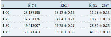
4.2.2 Changing
$\psi$

The expected loss $\tilde {\mathbb{E}}[C_t]$
, the CMC loss
$\tilde {\mathbb{E}}[C_t]$
, the CMC loss $\widehat {\tilde {\mathbb{E}}}[C_t]$
, and stop-loss
$\widehat {\tilde {\mathbb{E}}}[C_t]$
, and stop-loss $\widehat {\tilde {\mathbb{E}}}[(C_t - 25)^+]$
estimates (with 95% confidence intervals) for different values of the tilting parameter
$\widehat {\tilde {\mathbb{E}}}[(C_t - 25)^+]$
estimates (with 95% confidence intervals) for different values of the tilting parameter $\psi$
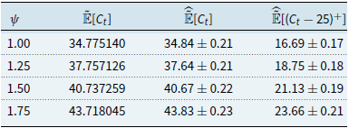
4.2.3 Changing
$\nu$

The expected loss $\tilde {\mathbb{E}}[C_t]$
, the CMC loss
$\tilde {\mathbb{E}}[C_t]$
, the CMC loss $\widehat {\tilde {\mathbb{E}}}[C_t]$
, and stop-loss
$\widehat {\tilde {\mathbb{E}}}[C_t]$
, and stop-loss $\widehat {\tilde {\mathbb{E}}}[(C_t - 25)^+]$
estimates (with 95% confidence intervals) for different values of the tilting parameter
$\widehat {\tilde {\mathbb{E}}}[(C_t - 25)^+]$
estimates (with 95% confidence intervals) for different values of the tilting parameter $\nu$
$\nu$
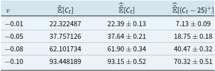
Comparing the numerical values in Table 2 with those in Table 3, the increases in gross insurance and reinsurance premium estimates due to changes in $\theta$
are greater than those resulting from changes in
$\theta$
are greater than those resulting from changes in $\psi$
. This is because
$\psi$
. This is because $\hat {j}(\nu )$
is involved in the self-exciting intensity function
$\hat {j}(\nu )$
is involved in the self-exciting intensity function $\lambda _{t}$
. Table 4 illustrates the increase in gross insurance and reinsurance premium estimates resulting from changes in
$\lambda _{t}$
. Table 4 illustrates the increase in gross insurance and reinsurance premium estimates resulting from changes in $\nu$
, which is due to both a higher self-exciting intensity and larger claim/loss sizes.
$\nu$
, which is due to both a higher self-exciting intensity and larger claim/loss sizes.
4.3 Sensitivity analysis for the intensity parameters
We next examine sensitivity with respect to the intensity parameters governing the dynamics of the claim arrival process. Using the same setup (i.e., the same baseline parameter values) as in the previous subsection, we focus on the mean $\widehat {\tilde {\mathbb{E}}}[C_t]$
and the stop-loss premium with retention
$\widehat {\tilde {\mathbb{E}}}[C_t]$
and the stop-loss premium with retention $L = 25$
.
$L = 25$
.
The following tables illustrate how these quantities change when key intensity parameters are varied individually, with all other parameters held constant (except $\phi$
, which is updated to satisfy
$\phi$
, which is updated to satisfy $\phi = -(\theta \hat {j}(\nu ) - 1)$
).
$\phi = -(\theta \hat {j}(\nu ) - 1)$
).
4.3.1 Changing
$\delta$

The expected loss $\tilde {\mathbb{E}}[C_t]$
, the CMC loss
$\tilde {\mathbb{E}}[C_t]$
, the CMC loss $\widehat {\tilde {\mathbb{E}}}[C_t]$
, and stop-loss
$\widehat {\tilde {\mathbb{E}}}[C_t]$
, and stop-loss $\widehat {\tilde {\mathbb{E}}}[(C_t - 25)^+]$
estimates (with 95% confidence intervals) for different values of the tilting parameter
$\widehat {\tilde {\mathbb{E}}}[(C_t - 25)^+]$
estimates (with 95% confidence intervals) for different values of the tilting parameter $\delta$
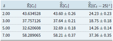
4.3.2 Changing
$\alpha$

The expected loss $\tilde {\mathbb{E}}[C_t]$
, the CMC loss
$\tilde {\mathbb{E}}[C_t]$
, the CMC loss $\widehat {\tilde {\mathbb{E}}}[C_t]$
, and stop-loss
$\widehat {\tilde {\mathbb{E}}}[C_t]$
, and stop-loss $\widehat {\tilde {\mathbb{E}}}[(C_t - 25)^+]$
estimates (with 95% confidence intervals) for different values of the tilting parameter
$\widehat {\tilde {\mathbb{E}}}[(C_t - 25)^+]$
estimates (with 95% confidence intervals) for different values of the tilting parameter $\alpha$

4.3.3 Changing
$\beta$

The expected loss $\tilde {\mathbb{E}}[C_t]$
, the CMC loss
$\tilde {\mathbb{E}}[C_t]$
, the CMC loss $\widehat {\tilde {\mathbb{E}}}[C_t]$
, and stop-loss
$\widehat {\tilde {\mathbb{E}}}[C_t]$
, and stop-loss $\widehat {\tilde {\mathbb{E}}}[(C_t - 25)^+]$
estimates (with 95% confidence intervals) for different values of the tilting parameter
$\widehat {\tilde {\mathbb{E}}}[(C_t - 25)^+]$
estimates (with 95% confidence intervals) for different values of the tilting parameter $\beta$
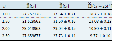
Table 5 shows the complicated relationship that $\delta$
has on the expected losses. Changing
$\delta$
has on the expected losses. Changing $\delta$
changes the solution
$\delta$
changes the solution $B(t)$
, and that changes nearly all of the Esscher-transformed parameters (except for claim sizes), making the impacts non-monotonic. Tables 6 and 7 present the reduction in them as the external-exciting and self-exciting jump size parameters
$B(t)$
, and that changes nearly all of the Esscher-transformed parameters (except for claim sizes), making the impacts non-monotonic. Tables 6 and 7 present the reduction in them as the external-exciting and self-exciting jump size parameters $\alpha$
and
$\alpha$
and $\beta$
increase. An increase in these jump size parameters results in a decrease in the exponential average.
$\beta$
increase. An increase in these jump size parameters results in a decrease in the exponential average.
4.4 Comparison with generalized Hawkes and shot-noise Cox processes
If there are no externally excited jumps in Eq. (2.2) (i.e., $\rho =0$
)
$\rho =0$
) $C_{t}$
becomes a generalized compound Hawkes process. If
$C_{t}$
becomes a generalized compound Hawkes process. If $a=0$
and there are no self-excited jumps in Eq. (2.2),
$a=0$
and there are no self-excited jumps in Eq. (2.2), $C_{t}$
becomes a compound Cox process with shot-noise Poisson intensity.
$C_{t}$
becomes a compound Cox process with shot-noise Poisson intensity.
The following two tables show the corresponding stop-loss CMC estimates in Table 1 (DCP case) for the generalized Hawkes case and the Cox case, respectively.
4.4.1 Generalized Hawkes process
The stop-loss CMC estimates $\widehat {\mathbb{E}}[(C_t - L)^+]$
under the original measure and
$\widehat {\mathbb{E}}[(C_t - L)^+]$
under the original measure and $\widehat {\tilde {\mathbb{E}}}[(C_t - L)^+]$
under the Esscher measure for different
$\widehat {\tilde {\mathbb{E}}}[(C_t - L)^+]$
under the Esscher measure for different $L$
retention levels. The point process driving
$L$
retention levels. The point process driving $C_t$
is a generalized Hawkes process
$C_t$
is a generalized Hawkes process
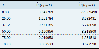
If we simulate using the same parameters as above, except setting $\rho = 0$
, then the underlying point process becomes a generalized Hawkes process.
$\rho = 0$
, then the underlying point process becomes a generalized Hawkes process.
4.4.2 Shot-noise Cox process
The stop-loss CMC estimates $\widehat {\mathbb{E}}[(C_t - L)^+]$
under the original measure and
$\widehat {\mathbb{E}}[(C_t - L)^+]$
under the original measure and $\widehat {\tilde {\mathbb{E}}}[(C_t - L)^+]$
under the Esscher measure for different
$\widehat {\tilde {\mathbb{E}}}[(C_t - L)^+]$
under the Esscher measure for different $L$
retention levels. The point process driving
$L$
retention levels. The point process driving $C_t$
is a shot-noise cox process
$C_t$
is a shot-noise cox process
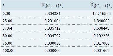
If we simulate using the same parameters as above, except setting $a = 0$
and
$a = 0$
and $\beta = \infty$
(i.e.,
$\beta = \infty$
(i.e., $Y_j \equiv 0$
for all
$Y_j \equiv 0$
for all $j$
), then the underlying point process becomes a shot-noise Cox process.
$j$
), then the underlying point process becomes a shot-noise Cox process.
Compared to Tables 8 and 9, Table 1 shows that gross insurance and reinsurance premium estimates significantly increase when changing $C_{t}$
from the Cox process with shot-noise Poisson intensity to a generalized Hawkes process due to self-excited jumps and to the dynamic contagion process due to both externally excited jumps and self-excited jumps.
$C_{t}$
from the Cox process with shot-noise Poisson intensity to a generalized Hawkes process due to self-excited jumps and to the dynamic contagion process due to both externally excited jumps and self-excited jumps.
5. Conclusion
The insurance sector is an important component of our economy, with trillions of dollars under management. We rely on well-functioning insurers. However, the current pricing mechanism for catastrophic risk insurance has put pressure on insurers and reinsurers when faced with more frequent and larger natural and man-made disasters. For example, in the aftermath of frequent natural disasters such as the 2022 South-East Queensland and New South Wales floods, many insurers only offer policies that include flood cover with approximately 30% increased premiums. Before the Southern California wildfires of January 2025, State Farm did not renew insurance policies in high-risk California postcodes due to increasing costs.
Unless (re)insurers have an appropriate framework and prudent methodology that adequately assess catastrophe risks, ordinary individuals and business owners will suffer, as the industry will not be able to promptly and fully meet the many claims of catastrophe victims. To address this challenge, in this paper, we presented how to obtain arbitrage-free catastrophe stop-loss reinsurance premiums when dealing with the ongoing challenge and complexity of emerging risk dynamics. To predict claim/loss arrivals from conventional and emerging catastrophes, we used the compound dynamic contagion process for the catastrophic component of the liability and the Esscher transform to determine arbitrage-free premiums. Sensitivity analyses were also performed by changing the retention level, the Esscher parameters, and the intensity parameters. Given the broad applicability of the CDCP, it is expected that what we have obtained in this paper will provide practitioners with feasible approaches to quantify their catastrophic liabilities in light of the growing challenges posed by new risks arising from climate change, cyberattacks, and pandemics. We also envisage that the dynamics used in this paper extend naturally for pricing a variety of catastrophe insurance derivatives. For this, we leave them as objects of further research.
Data availability statement
The Python code used to generate the numerical results is available at: https://github.com/Pat-Laub/ReinsuranceEsscherDynamicContagion.
Funding statement
This work received no specific grant from any funding agency, commercial or not-for-profit sectors.
Competing interests
The authors declare none.
Appendix A. Equivalent martingale measure with non-zero interest rate
Definition 6 (Equivalent martingale measure with discounting). Let $r \ge 0$
be a constant risk-free interest rate. A probability measure
$r \ge 0$
be a constant risk-free interest rate. A probability measure $\tilde {\mathbb{P}}$
is said to be an equivalent martingale probability measure (i.e.,
$\tilde {\mathbb{P}}$
is said to be an equivalent martingale probability measure (i.e., $\tilde {\mathbb{P}}$
is equivalent to
$\tilde {\mathbb{P}}$
is equivalent to $\mathbb{P}$
on
$\mathbb{P}$
on $\mathcal{F}_T$
) if it satisfies the following properties:
$\mathcal{F}_T$
) if it satisfies the following properties:
-
(i)
$\tilde {\mathbb{P}}(A)=0$
if and only if
$\mathbb{P}(A)=0$
for any
$A \in \mathcal{F}_T$
; -
(ii) The Radon–Nikodym derivative
$\frac {\mathop {}\!\mathrm{d} \tilde {\mathbb{P}}}{\mathop {}\!\mathrm{d} \mathbb{P}} \in L^{2}(\Omega , \mathcal{F}_{T}, \mathbb{P})$
; -
(iii) The discounted surplus process
$\{ \mathrm{e}^{-rt} R_t \}_{t \in \mathcal{T}}$
is an
$(\mathbb{F}, \tilde {\mathbb{P}})$
-martingale. In particular,
\begin{equation*} \tilde {\mathbb{E}}\!\left [ \mathrm{e}^{-rt} R_t \mid \mathcal{F}_s \right ] = \mathrm{e}^{-rs} R_s, \qquad 0 \le s \le t \le T, \quad \tilde {\mathbb{P}}\text{-a.s.} \end{equation*}


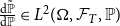


Remark 2. Assuming $R_0=0$
, Definition 6 (iii) implies
$R_0=0$
, Definition 6 (iii) implies
 \begin{equation*} \tilde {\mathbb{E}}\!\left ( \mathrm{e}^{-rt} R_t \mid \mathcal{F}_0 \right ) = \tilde {\mathbb{E}}\!\left ( \mathrm{e}^{-rt} (P_t - C_t) \mid \mathcal{F}_0 \right ) =0. \end{equation*}
Consequently,
 \begin{equation*} \tilde {\mathbb{E}}\!\left ( \mathrm{e}^{-rt} C_t \mid \mathcal{F}_0 \right ) = \tilde {\mathbb{E}}\!\left ( \mathrm{e}^{-rt} P_t \mid \mathcal{F}_0 \right)\!, \end{equation*}
which characterizes the arbitrage-free insurance premium under a non-zero constant interest rate.
Appendix B. Simulation algorithms
Algorithm 2 shows our method for simulating the time-inhomogeneous compound dynamic contagion process, which extends the work of Ogata (Reference Ogata1981). It utilizes Algorithm 1 which is the well-known thinning algorithm for Poisson processes (see Lewis & Shedler, Reference Lewis and Shedler1979).
Simulate a time-inhomogeneous Poisson process

In the next algorithm we split the terms in Eq. (2.5) into
 \begin{equation} \lambda _{t} = \underbrace {{\lambda _0 \mathrm{e}^{-\delta t} + \delta \int _{0}^{t} a(s) \mathrm{e}^{-\delta (t-s)} \, \mathop {}\!\mathrm{d} s} + \sum _{i \ge 1} X_{i} \mathrm{e}^{-\delta \left ( t - T_{1, i} \right )}\mathbb{I}_{\{ T_{1,i} \le t \}} }_{=: \lambda ^{(c)}_t , \text{ the ``Cox'' part}} + \underbrace {\sum _{j \ge 1} Y_{j} \mathrm{e}^{-\delta \left (t - T_{2,j} \right )} \mathbb{I}_{ \{ T_{2, j} \le t \}}}_{=: \lambda ^{(h)}_t , \text{ the ``Hawkes'' part}} . \end{equation}
Simulate a time-inhomogeneous compound dynamic contagion process
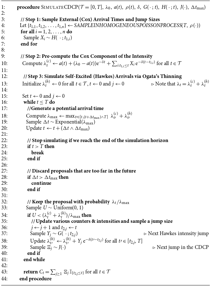
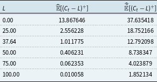
 E^[(Ct−L)+]
 E~^[(Ct−L)+]
 L
L
 Ct
Ct λt
λt P
P P~
P~ P~
P~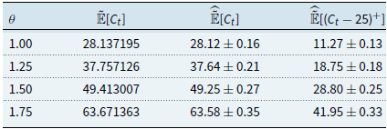
 E~[Ct]
 E~^[Ct]
 E~^[(Ct−25)+]
 θ
θ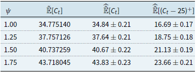
 E~[Ct]
 E~^[Ct]
 E~^[(Ct−25)+]
 ψ
ψ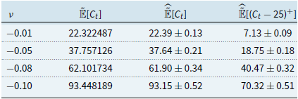
 E~[Ct]
 E~^[Ct]
 E~^[(Ct−25)+]
 ν
ν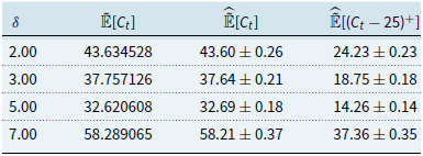
 E~[Ct]
 E~^[Ct]
 E~^[(Ct−25)+]
 δ
δ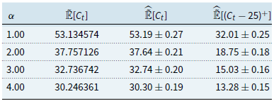
 E~[Ct]
 E~^[Ct]
 E~^[(Ct−25)+]
 α
α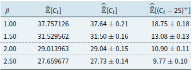
 E~[Ct]
 E~^[Ct]
 E~^[(Ct−25)+]
 β
β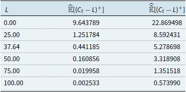
 E^[(Ct−L)+]
 E~^[(Ct−L)+]
 L
L Ct
Ct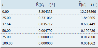
 E^[(Ct−L)+]
 E~^[(Ct−L)+]
 L
L Ct
Ct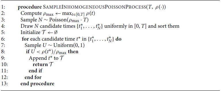
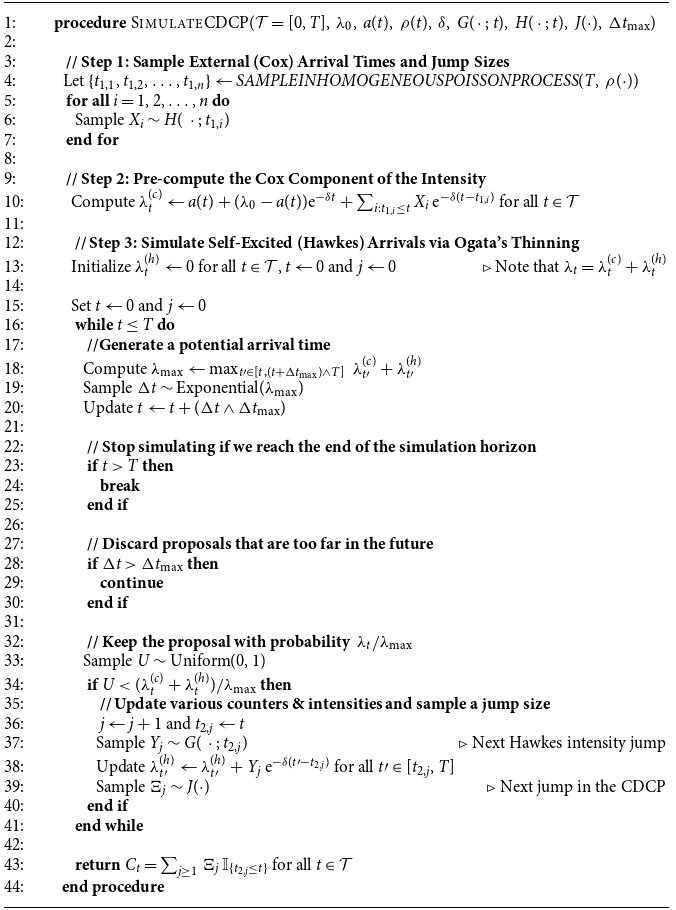

 Open access

