


1. INTRODUCTION
Glacier ice thickness distribution and bedrock topography are important basic parameters for a number of applications, such as ice volume estimation (e.g. Navarro and others, Reference Navarro2014), modeling of future glacier dynamics (Zekollari and others, Reference Zekollari, Fürst and Huybrechts2014), hydrological projections (Gabbi and others, Reference Gabbi, Farinotti, Bauder and Maurer2012), studies of glacier-related hazards and glacial lake formation (Vincent and others, Reference Vincent, Descloitres, Gilbert and Legchenko2012), and ice core studies (Eisen and others, Reference Eisen, Nixdorf, Keck and Wagenbach2003) among many others. Despite their importance, ice thickness measurements are limited, mainly due to logistical difficulties. This is especially true for the most remote and high-altitude glaciers. A recent compilation of available ice thickness data shows that detailed glacier-wide thickness measurements are available for only ~550 glaciers (Gärtner-Roer and others, Reference Gärtner-Roer2014, Reference Gärtner-Roer2016).
A number of attempts have been made to model glacier ice thickness based on surface topography, mass balance, ice flow velocities and theoretical assumptions. Recent model comparisons show discrepancies, especially for ice caps, and indicate a high demand for detailed glacier ice thickness data against which the models can be calibrated and validated (Farinotti and others, Reference Farinotti2017).
Ground-penetrating radar (GPR) is a geophysical method widely used for various glaciological applications (Navarro and Eisen, Reference Navarro and Eisen2009). It is based on registering electromagnetic wave reflections from internal glacier features and bedrock. Two primary research goals in glaciological GPR studies are measurements of ice thickness and evaluation of glacier internal structure (Dowdeswell and Evans, Reference Dowdeswell and Evans2004). Besides its scientific and practical importance, knowledge of these parameters is essential for paleoglaciological studies and ice flow modeling. The value of including GPR in alpine glacier coring investigations has been demonstrated by studies in the Swiss Alps (Eisen and others, Reference Eisen, Nixdorf, Keck and Wagenbach2003), Caucasus (Mikhalenko and others, Reference Mikhalenko2015) and most recently on Kilimanjaro (Bohleber and others, Reference Bohleber2017).
Bedrock topography information and englacial layering are crucial for selecting deep ice core drilling sites as well as interpretation of ice core records (Konrad and others, Reference Konrad, Bohleber, Wagenbach, Vincent and Eisen2013). Data on bedrock topography and internal structure of the Colle Gnifetti glacier in the Swiss Alps enabled 3-D internal age distribution modeling (Eisen and others, Reference Eisen, Nixdorf, Keck and Wagenbach2003; Konrad and others, Reference Konrad, Bohleber, Wagenbach, Vincent and Eisen2013). The internal reflections are considered to be from layers initially formed on the glacier surface. These isochronal layers can be used to connect separate ice core records, estimate accumulation distribution, and calibrate age/depth relationships (Pälli and others, Reference Pälli2002; Konrad and others, Reference Konrad, Bohleber, Wagenbach, Vincent and Eisen2013; Sold and others, Reference Sold, Huss, Eichler, Schwikowski and Hoelzle2015; Bohleber and others, Reference Bohleber2017). The high mountain drilling sites can be very difficult to model as the variations in ice depth and snow accumulation can reach orders of magnitude within very short distances. Reliable modeling of the age/depth relationship and its distribution require accurate ice thickness and bedrock topography data.
The Tibetan Plateau, often referred to as the Third Pole, and its surrounding mountains accommodate the largest number of glaciers outside the Polar Regions, with a total glacial area of 100 000 km2 (Yao and others, Reference Yao2012a). Its geographical location, size, and elevation define the major impact of the Third Pole on large scale atmospheric circulation patterns (Yao and others, Reference Yao2012a). Considerable effort has been applied toward glacier monitoring in Central Asia and on the Tibetan Plateau in particular (Bolch and others, Reference Bolch2012; Yao and others, Reference Yao2012b; Sorg and others, Reference Sorg, Bolch, Stoffel, Solomina and Beniston2012; Neckel and others, Reference Neckel, Kropáček, Bolch and Hochschild2014; Yi and Sun, Reference Yi and Sun2014; Farinotti and others, Reference Farinotti2015; Ye and others, Reference Ye2017). However, glacier wide data on ice thickness are still very limited due to remote locations and extremely high elevations. Ice thickness datasets exist for selected glaciers in the Tien Shan, Urumqi Glacier No. 1 (Wang and others, Reference Wang2014), the central Tibetan Plateau, Qiangtang glacier (Zhu and others, Reference Zhu, Tian, Wang and Cui2014), Muz Taw glacier in the Sawir Mountains (Baojuan and others, Reference Baojuan2015) and the southern Tibetan Plateau (Tian and others, Reference Tian2014).
The Guliya ice cap in the western Kunlun Mountains is the highest and largest (total area of 376 km2, flat-top area of 132 km2) ice cap in the mid to low latitudes (Yao and others, Reference Yao, Jiao, Zhang, Yang and Thompson1992). It is characterized by extremely cold, polar-like conditions (Thompson and others, Reference Thompson1995). A deep drilling program conducted in the summer of 1992 resulted in the longest ice core climate record outside the Polar Regions (~130 000 years), and showed that even older ice is preserved in the deepest layers of the glacier (Thompson and others, Reference Thompson1997). Prior to the 1992 drilling program, field studies were conducted in 1990 and 1991 which included surface accumulation measurements, shallow core and snow pit sampling and surface ice flow velocity measurements. Ice thickness was measured around the ice cap at several discrete points with a short-pulse radar operating using a central frequency of 10 MHz. Thompson and others (Reference Thompson1995, Reference Thompson1997) and Yao and others (Reference Yao, Jiao, Zhang, Yang and Thompson1992) provided detailed descriptions of the field measurements and laboratory methods used in climatic and environmental studies of the Guliya ice cap.
In this paper, we present detailed ice thickness measurements conducted on the Guliya ice cap using GPR during a drilling campaign in 2015. The total length of GPR profiles on the Guliya ice cap was ~80 km, making it one of the largest ice thickness datasets in Central Asia. The results of the GPR measurements were compared with the borehole depth and ice core stratigraphy. We assessed surface elevation changes of the ice cap and neighboring glaciers from 2000 to 2015.
2. DATA COLLECTION AND PROCESSING
The Guliya ice cap is located on the western edge of the Tibetan Plateau in far western Kunlun Shan, China. It spans an elevation range of 1000 m, with its summit at 6650 m a.s.l. Most of the surface consists of flat areas with an average slope of <3–5°; however the slope increases toward the summit and the north-east where a large outlet glacier is located.
In September and October of 2015 a geophysical survey was conducted in two areas covering a total area of ~18 km2 located on the Guliya Plateau (GP) and the Guliya Summit (GS) near the ice core drilling sites (Fig. 1). The main dataset, consisting of ~70 km of GPR profiles, was obtained from the GP (5900–6200 m a.s.l.) with denser profiling conducted in the vicinity of the drilling site (35°13′58.8″N, 81°28′5.729″E). Profiles around the GS drilling site (35°17′22.474″N, 81°29′43.979″E) cover the elevation range of 6590–6650 m a.s.l.
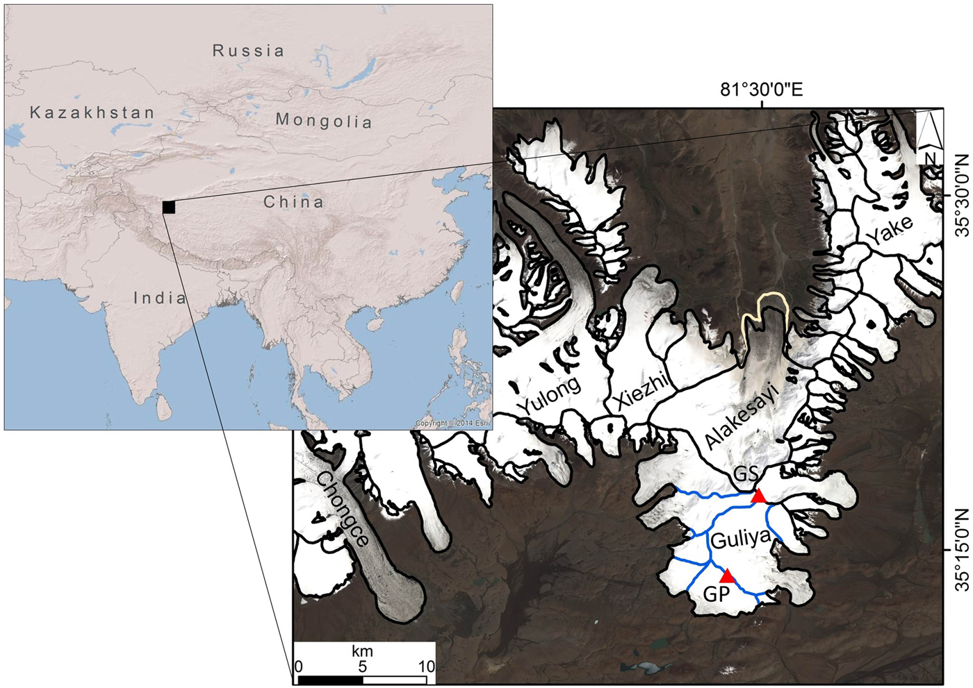
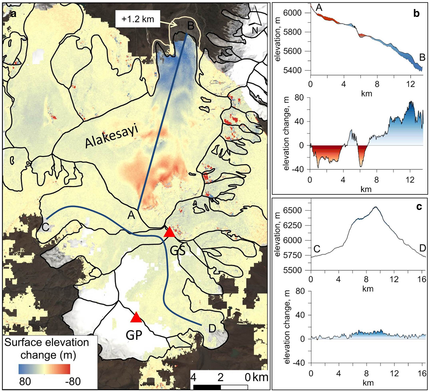
Location of the Guliya ice cap and ice core drilling sites (red triangles). The image of the icefield, of which Guliya is a part, is a Sentinel-2A image from 08 August 2017. The RGI 6.0 glacier outlines (RGI Consortium, 2017) are shown in black, ice drainage basins of the Guliya ice cap are shown in blue. Note the Alakesayi glacier advance, outlined in white, in 2015–2017. Map created using ArcGIS® software by Esri.
For ice thickness measurements we used commercial high-performance GPR manufactured by Geophysical Survey Systems Incorporated (GSSI). Such a radar is widely used in glaciological applications, both in the polar and in alpine regions (e.g. Shean and Marchant, Reference Shean and Marchant2010; Singh and others, Reference Singh, Rathore, Bahuguna, Ramnathan and Karthic2012; Kehrl and others, Reference Kehrl, Hawley, Osterberg, Winski and Lee2014). The 3200 Multiple Low Frequency Antennas with a center frequency of ~20 and 40 MHz were used for the survey at the GP and GS sites, respectively. The antenna is composed of two fully extended (240 cm for 20 MHz and 120 cm for 40 MHz) telescopic antenna elements on both the receiver and transmitter. Data were collected in continuous profile mode. The GPR system was mounted on two sleds, which were towed by snowmobile at an average speed of 10 km h−1. The antennas were positioned 30–40 cm above the surface on a wooden frame that rested on the plastic sleds (Fig. 2). Some noise might have been introduced by the operation on the rough glacier surface. The offset between antennas was limited by the standard cable length to 4 m. The antennas were arranged parallel to each other and perpendicular to the profiling direction. In such a configuration, the larger coupling between antennas may be expected (Navarro and Eisen, Reference Navarro and Eisen2009). Radar traces and GPS coordinates were recorded simultaneously. Conventional GPS with the nominal horizontal positioning accuracy of ±5 m was used. Due to low air temperatures, battery lifetime was reduced by ~50%; however, we did not detect any overheating problems with the device, which are common when operating at elevations above 6000 m.
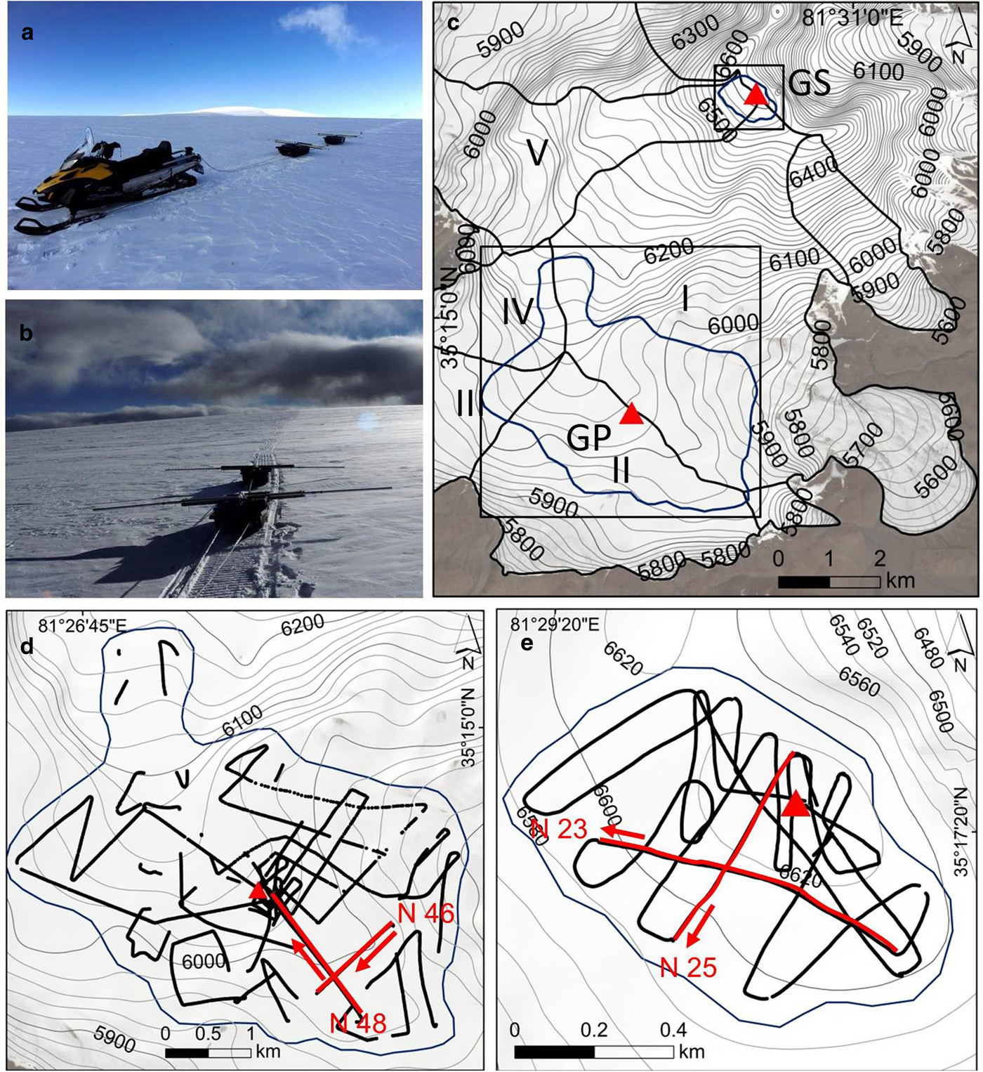
(a, b) Photos showing measurement logistics on the GP. (c) Location of the GPR survey sites (blue lines), drilling sites (red triangles), surface topography and Guliya glacier basins (black outlines and numbers). GPR measurement profiles at the (d) GP and (e) GS sites. Background image is a Sentinel-2A image from 08 August 2017. Location and orientation of selected profiles discussed in the text are shown by red lines and red arrows, respectively.
After the radar data (radargrams) were collected, they were processed using Radan 7 software and exported to text format for further implementation in GIS. Data were obtained with the predefined parameters: continuous time survey mode, 32-bit data format, 256 samples per scan. Time/depth range varied between 2000 (GS) and 6000 (GP) ns. The processing steps included static correction to eliminate air wave reflections; bandpass filtering to improve the signal-to-noise ratio and to reduce high-frequency and low-frequency noise; background removal filter and a signal amplification filter (gain function) to account for signal loss with depth. Geometrical irregularities were corrected using Kirchhoff Migration method in RADAN 7 software. Profiles were digitized manually using the layer-picking mode to select the reflection arrival time from the ice/bed interface. The two-way travel time was then converted into ice thickness depending on the radio wave velocity (RWV).
2.1. RWV calculation
The theory of radio-wave propagation in glacier ice is described in detail elsewhere (e.g. Macheret, Reference Macheret2006; Navarro and Eisen, Reference Navarro and Eisen2009). The best way to estimate the electromagnetic wave propagation velocity is to use common midpoint measurements. Unfortunately, these were not available; therefore, we used information about the underlying media provided by the ice core analysis.
The permittivity of snow, firn and ice to radio waves in the absence of liquid water depends mostly on density. Various empirical formulas and mixture models are used to estimate the mean permittivity of ice (ε) (Looyenga, Reference Looyenga1965; Robin, Reference Robin1975). Another approach is to use the inversion of reflection amplitudes to compute the series of reflection coefficients that can be used to estimate the wave velocity in a depth interval within the glacier (Forte and others, Reference Forte, Dossi, Pipan and Colucci2014). Given the low temperatures throughout the glacier body, the absence of meltwater, and the very thin firn layer at the GP site, we used the constant propagation wave velocity of 0.168 m ns−1 for the dry ice (Dowdeswell and Evans, Reference Dowdeswell and Evans2004).
At the GS drilling site, the presence of a thick firn cover prompted the use of the relationship determined by Kovacs and others (Reference Kovacs, Gow and Morey1995) to calculate RWV and to account for the density dependence of the electric permittivity of ice and firn:
 $$\varepsilon = (1 + 0.000845\rho )^2$$
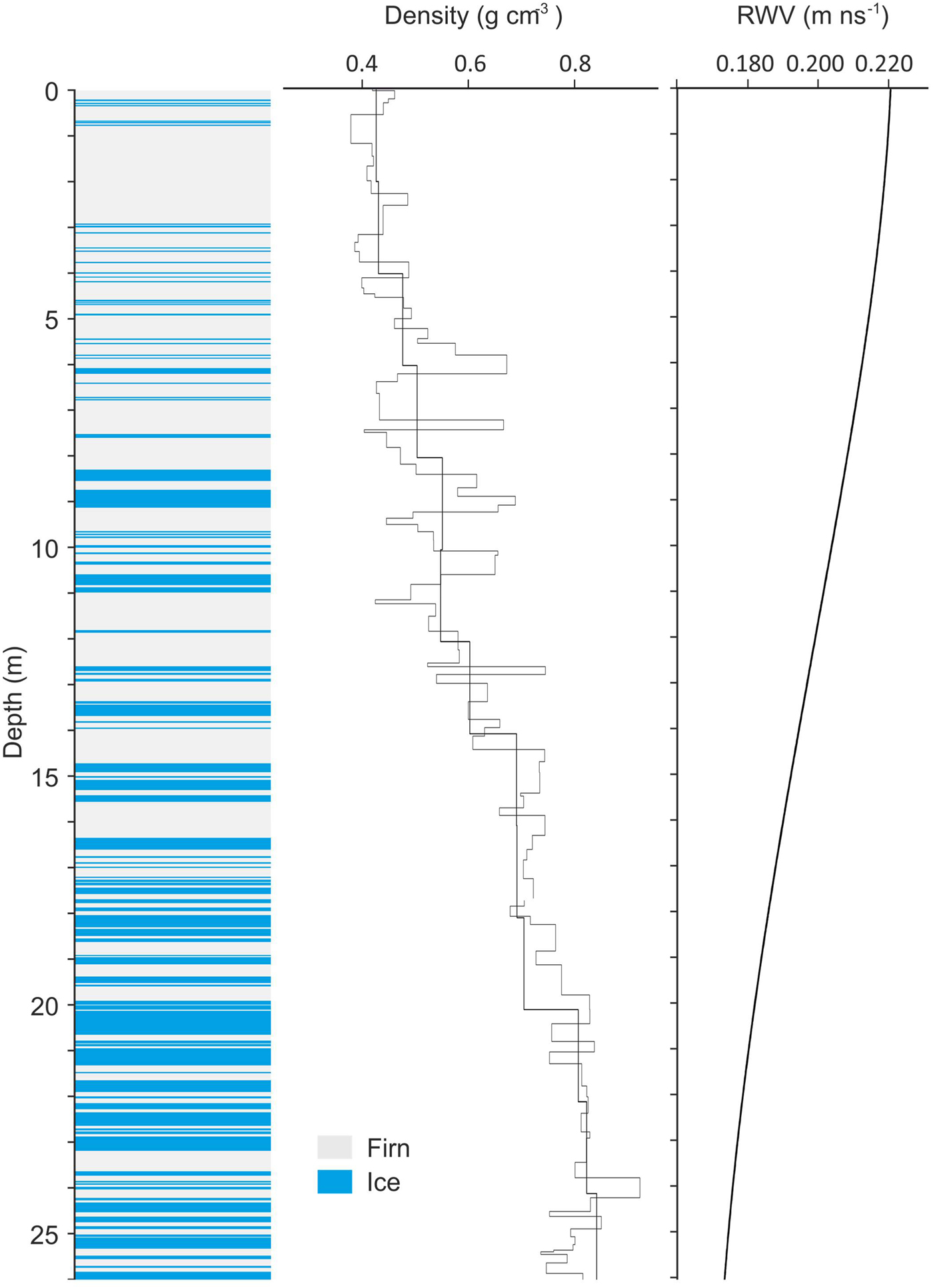
where the density ρ is in kg m−3. The permittivity ε was calculated for the upper 26 m at the GS drilling site using Eqn (1) and a third-order polynomial approximation of the density profile obtained from ice core analysis. The mean RWV (u) was then computed as u = cε −0.5. Below 26 m depth, we used a constant velocity of 0.168 m ns−1 (Fig. 3). The assumption was made that density variations within the firn cover are similar throughout the GPR survey area.
Stratigraphy, bulk density, and 2 m average and calculated radio wave propagation velocity for the upper 26 m at the GS drilling site (6650 m) of Guliya glacier.
2.2. Ice thickness interpolation
Ice thickness maps were created by interpolating ice thickness point data to a regular grid. Traditionally, the GPR data are interpolated by the means of probabilistic methods such as ordinary kriging. This method is not only used for data interpolation but also can be applied to predict interpolation uncertainty. Because we assume that the physical properties of the firn and ice do not vary with horizontal position and if only one semivariogram is used for all the observations, the ordinary kriging method then underestimates the interpolation error of the ice thickness data (Lapazaran and others, Reference Lapazaran, Otero, Martin-Español and Navarro2016a). Here we used an empirical Bayesian kriging (EBK) method for ice thickness interpolation and uncertainty assessment. This is a standard tool implemented in ArcGIS Geostatistical Analyst. Unlike classical kriging, the EBK accounts for the semivariogram model errors by automated subsetting of the observations and numerous repeated semivariogram model calculations. The resulting distribution of semivariograms is then used to predict values in unsampled locations and estimate prediction errors (Krivoruchko, Reference Krivoruchko2012). The EBK method solves the problem of cross validation and underestimation of the interpolation error for the unevenly distributed GPR data and can be utilized with large data sets, which make it a useful tool for GPR measurements.
We used the following EBK parameters for interpolation of GP and GS ice thickness datasets: empirical transformation, K-Bessel semivariogram model, the subset size of 200 points for GP and 100 points for GS, an overlap factor of 3, and the number of simulations were set to 100. For each site, the prediction and prediction errors maps were produced.
2.3. Surface and basal topography
In order to construct the basal topography map, the glacier surface elevation is required. The High Mountain Asia (HMA) 8-meter Digital Elevation Model (DEM) dataset generated from very-high-resolution imagery (0.5 m) from DigitalGlobe Inc. (available from the NASA National Snow and Ice Data Center Distributed Active Archive Center (https://nsidc.org/data/highmountainasia) was used as a source of topographic data for the GS site. A HMA DEM image acquired on 20 August 2015 was made available from the WORLDVIEW-1 imagery (Shean, Reference Shean2017). For the GP site, gaps in HMA DEM were detected, which were filled by the Shuttle Radar Topography Mission X-band DEMs (http://eoweb.dlr.de:8080/free_SRTM_X-band_data.html) in 1-arc resolution, provided by the German Aerospace Centre (DLR). These DEMs were also used to estimate elevation changes. Co-registration and vertical biases were assessed using an approach based on the relationship of the resulting elevation differences with terrain slope and aspect over non-glacier areas (Nuth and Kääb, Reference Nuth and Kääb2011). The HMA DEM was resampled to a 30 m resolution and elevation differences of more than 100 m were discarded. The comparison between two DEMs for 17 513 pixels over non-glaciated areas resulted in std dev. of 3.62 m. In order to construct the surface DEM for the GP site, the HMA DEM voids were filled with the SRTM-X DEM values which were corrected to account for an average elevation change over the Guliya glacier during the 2000–2015 period. The bed topography was calculated by subtracting the interpolated ice thickness values from the glacier surface DEM.
3. ERROR ESTIMATION
The accuracy of the ice thickness and bedrock topography was estimated following the approach and considerations published in a recent comprehensive review of errors involved in ice thickness estimations (Lapazaran and others, Reference Lapazaran, Otero, Martin-Español and Navarro2016a, Reference Lapazaran, Otero, Martín-Español and Navarrob). The total error of gridded bedrock topography results from two major sources: errors in ice thickness DEM and surface DEM uncertainties. Ice thickness DEM accuracy depends on errors in GPR point measurements errors and interpolation errors. We analyzed each of these components separately for the GS and GP sites.
3.1. Ice thickness measurement errors
The total error of the GPR ice thickness estimation at a given point consists of two components: the error inherent in the measurements, and the horizontal positioning uncertainty (Lapazaran and others, Reference Lapazaran, Otero, Martin-Español and Navarro2016a). Measurement error is related to the chosen time-to-depth conversion (ε c) and to the reflection picking accuracy or timing error (ε τ).
The differences between ice-thicknesses at the intersections of GPR profiles were analyzed to estimate the quality and consistency of the radar data obtained during the fieldwork. The statistics of the intersection differences illustrate the uncertainty in the radar data (e.g. Bamber and others, Reference Bamber2013; Martín-Español and others, Reference Martín-Español2013; Saintenoy and others, Reference Saintenoy2013). Since the measurements presented here were completed during one field campaign, the discrepancies at the intersections should be similar to the ice thickness errors (Navarro and others, Reference Navarro2014). However, it should be noted that while this tool provides insight into the presence of some inconsistencies, it does not allow accurate assessment of errors and serves only as an approximation. The std dev. of the intersection absolute differences for the GP site was 6.9 m, with a mean value of 7.2 m or 3% of the mean measured ice thickness. For the GS site std dev. was 1.1 m and the mean difference was 2.3 m or 3.6%.
To account for spatial variations of the RWV, a 2% uncertainty (ε c) is assumed for both sites based on information of the underlying media properties from the ice cores analyses and borehole temperatures (Navarro and Eisen, Reference Navarro and Eisen2009; Lapazaran and others, Reference Lapazaran, Otero, Martin-Español and Navarro2016a).
An additional error may be introduced to the RWV calculation at the GS site by the assumption of a uniform firn–ice transition depth throughout the survey area. Errors of total ice thickness estimation increase with the firn layer thickness (Babenko and Macheret, Reference Babenko and Macheret1997; Macheret, Reference Macheret2006). The radargrams of the GS site show that the estimated maximum firn thickness was 35–40 m for the deepest parts. Since the difference in total ice thickness calculated by using the constant or variable firn–ice transition zone at the GS site was ~1 m, this error may be neglected.
Timing error ε τ is related to the GPR resolution and includes errors in interpretation of the bed reflections. The latter can be evaluated from the central frequency as ε τ = 1/f, which is equivalent to half of the wavelength in terms of ice thickness. We used 20 MHz antennas for the GP drilling site and 40 MHz antennas for the GS site, which resulted in ε τ values of 4.2 m and 2.1 m, respectively, assuming the constant RWV of 0.168 m ns−1.
The additional uncertainty of the ice thickness estimation occurs from the horizontal-positioning error of each GPR trace. This error depends on the accuracy of the GPS positioning and traces positioning error due to GPR movement. To account for such uncertainties we used the approach described in detail in Lapazaran and others (Reference Lapazaran, Otero, Martin-Español and Navarro2016a). The positioning error of stand-alone GPS was assumed to be 5 m and the positioning error due to GPR movement was estimated as 1.39 m since the time step between subsequent traces was set to 1 s. This results in a total positioning error of 5 m. To estimate the positioning-related ice thickness error, we calculated differences between measured ice thicknesses values located within a circle of 5 m radius from each other. The maximum discrepancies of 3.94 and 9.84 m were found at the GS and GP sites, respectively.
The resulting total GPR ice thickness measurement error was calculated for each data point. For the GS site, this produced values between 4.48 and 4.84 m with a mean of 4.61 m and std dev. of 0.09 m. For the GP site, values of the total ice thickness measurement error varied between 10.82 and 13.02 m with a mean of 11.69 m and std dev. of 0.47 m (Table 1).
GPR ice thickness measurement errors (see the text for explanation)

3.2. Ice thickness interpolation errors
Prediction of standard errors was made using an EBK (Krivoruchko, Reference Krivoruchko2012). The cross-validation analysis showed that the EBK interpolation resulted in a root mean square error of 4.77 m for 5872 measurements at the GP site and 0.93 m for 1439 measurements the GS site. A prediction standard error map was calculated for both study areas. The average interpolation error for the GP area was 18.38 m with the std dev. of 11.75 and maximum of 73 m (Table 1). The errors propagate depending on the spatial density of the profiles, and the largest errors correspond to the areas with the least data coverage. The largest uncertainties were estimated in the north-west part of the GP site where the distance between the GPR profiles was several hundred meters. Therefore, at this location the uncertainty in ice thickness is about one-third of the ice thickness values. Another source of uncertainty is large variations in ice thicknesses over short distances. Such deviations were well described by the EBK method. Evenly distributed ice thickness measurement profiles at the summit provided more accurate interpolation, with an average error of 2.34 m, std dev. of 1.9 m, and maximum of 9.67 m. Following suggestions in Lapazaran and others (Reference Lapazaran, Otero, Martin-Español and Navarro2016a), errors in ice thickness at the data points were propagated to each grid by the means of kriging interpolation, which was applied to errors instead of ice thicknesses. The distribution of propagated errors was then combined with the interpolation errors as the root of their squared sum in each gridpoint providing the total ice-thickness error (Table 1; Figs 6b, 7b).
3.3. Basal topography errors
The total error in basal elevation at a given gridcell was calculated as a root mean square of the ice thickness grid and surface elevation DEM errors. The HMA-8 DEM acquired with the WorldView-1 along-track pairs have a horizontal/vertical accuracy of <5 m with the relative error of 1–2 m (Shean, Reference Shean2017). SRTM X-band signal penetration can be considered negligible for the glaciers outside dry recrystallization zones (Gardelle and others, Reference Gardelle, Berthier and Arnaud2012). We consider std dev. of the DEMs difference for the non-glacier areas (3.62 m) as an uncertainty estimate for the DEM difference within the glacier.
4. RESULTS AND DISCUSSION
During the 2015 Guliya expedition, four ice cores were drilled to bedrock successfully. The longest core (309.72 m) was drilled on the GP using an electromechanical corer in a dry borehole. Here the firn/ice transition occurred in a surface layer of only 20–30 cm thickness. Ice temperatures were −11.9, −6 and −2.1°C at 15, 200 and 309.72 m, respectively. Three cores to bedrock (50.72, 51.38 and 50.86 m) were obtained from the GS within 5 m of each other. GS ice core stratigraphy in the upper ~26 m consists of firn with numerous ice layers ranging from 1 to 33 cm thickness. Below the firn/ice transition, the cores are composed of glacier ice. The temperature profile in one of the boreholes shows a steady increase from −17.2°C at 10 m depth to −15°C at the bottom (51 m).
Examples of a typical radargrams for the GP site are shown in Figure 4. Radar data obtained with the 20 MHz frequency at the GP site did not reveal any continuous internal reflections; however, the low frequency enabled ice/bed interface detection of the deeper (>300 m) parts. The basal reflections can be clearly seen at both profiles. We did not detect any point-like reflectors or areas of significant radar signal scattering within the GP site which confirms the cold englacial thermal regime.
Typical examples of initial GPR radargrams (not topographically corrected) profiles (a) N48 and (b) N46 on the GP. (c) 3D view of radargrams. Location and orientation of the profiles are shown in Fig. 2d.
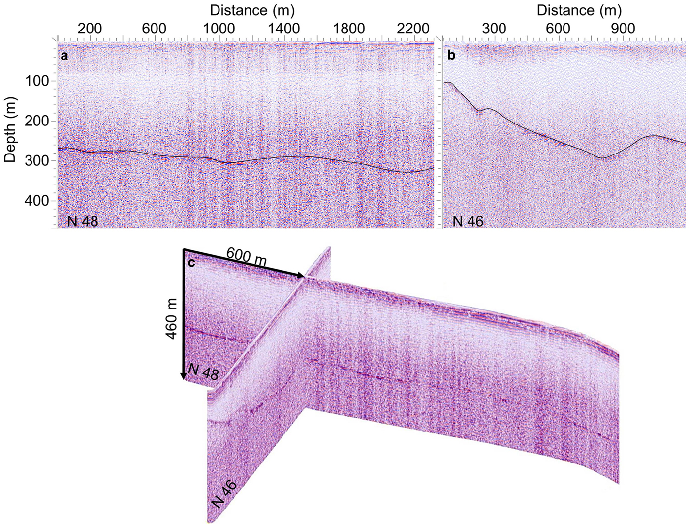
Figure 5 shows the measured ice thicknesses and basal topography around the GP site. The ice thickness measured 10–15 m from the GP drilling site was 306 ± 12.33 and 312 ± 12.39 m for different profiles, which differed by <4 m from the borehole depth (309.73 m), thus legitimizing the use of the constant RWV of 0.168 m ns−1 for the GP site. The maximum ice thickness of 371.12 ± 13.02 m was measured at 1.3 km north-west of the GP drilling site. The mean measured ice thickness at the GP site was 228.76 ± 11.69 m (Fig. 5c, d).
(a) Surface topography, glacier ice drainage basins (black lines) and ice flow direction (arrows), GPR measurement GP site outline (blue line). (b) Total ice thickness error map for the GP site. (c) Ice thickness and (d) basal topography on the GP. Surface and basal topography at cross sections (e) A-B and (f) C-D are shown.
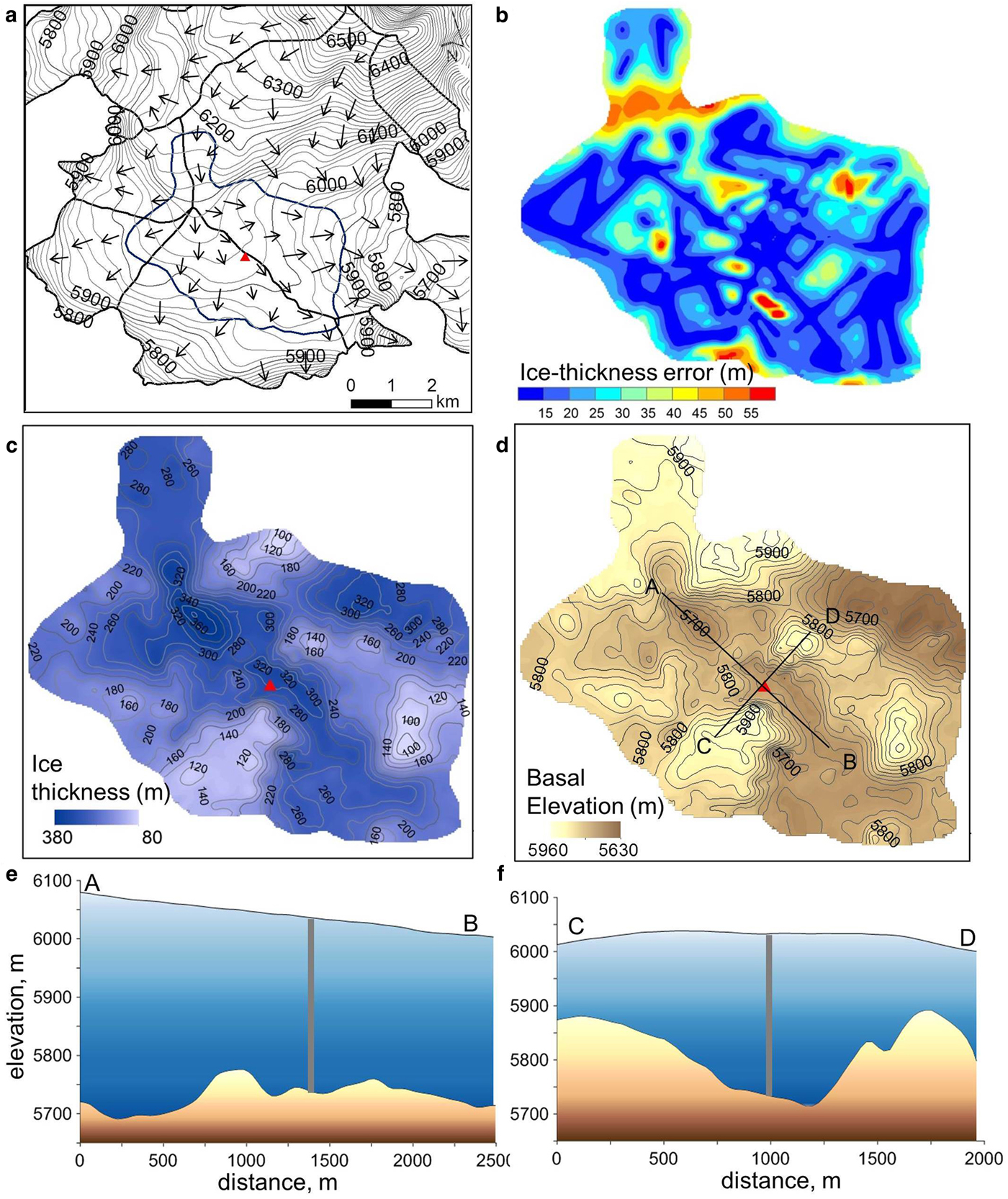
Ice flow direction and glacier drainage basins were determined using a hydrological analysis of the surface topography in ArcGIS. Guliya ice cap can be separated into five major basins (see Fig. 2). The GP drilling site is located at the ice divide between two basins (I and II) where the ice stream from the higher elevations diverges to the east and the south. The surface topography reveals a gentle slope of 1.5–2° along the ice divide. Basal topography maps based on the measured ice thicknesses reveal a complex bed (Fig. 5d). The longitudinal profile A-B in the NW to SE u-shaped subglacial valley in which the deep borehole is located is shown in Fig. 5e. The deepest depression, with an ice thickness of 370 m, is located 1.5 km upstream and a 35–40 m high ridge lies between the depression and the drilling site. Another valley with much steeper slopes lies to the east of this depression, and here the ice flow is faster due to a sharp elevation drop, which was confirmed by the surface topography and presence of crevasses. Figure 5f shows the cross section C-D from SW to NE over the GP drilling site. Over a distance of 0.5 km, the ice depth changes from 320 to 150 m, which illustrates the ruggedness of the bedrock. A relative rise of the surface by ~15 m occurs ~1 km from the borehole, despite the fact that this ice divide was positioned along the 100–140 m deep subglacial valley.
Sites suitable for drilling older ice cores are characterized by low ice accumulation rates, small flow velocity and high ice thickness and absence of ice flow disturbances. The surface topography and ice thickness distribution described above suggest low horizontal ice flux at the GP site. Subglacial relief is not reflected in surface topography; instead, the ice surface rise is observed at the ice divide, which is similar to the situation on polar ice caps. Deeper parts of the glacier were identified upstream from the GP site. But the steeper slopes together with the presence of the crevasses on the surface indicate faster ice flow at this location. This area is also an ice-divide between four ice drainage basins with a constant inflow of ice from the upper parts. The GP drilling site in contrast is located lower and the surface topography together with cold basal conditions suggest relatively slow ice flow in one direction following the subglacial valley. Overall the assessment of the surface and basal topography confirms suitability of the chosen ice core drilling site.
The internal reflections are shown on the 40 MHz profiles obtained on the summit (Fig. 6). The GPR profiles from the drilling site reveal multiple continuous reflectors within the upper 25–28 m (280–320 ns) (Fig. 6c). The lower part of the radargrams did not show any strong reflections from the internal layers, which is indicative of the complete firn–ice transition and a uniform ice density distribution. This conclusion is confirmed by the density measurements and stratigraphy analysis of the GS cores (Fig. 3). The high-resolution density profile shows large variations in the top 13–15 m in which numerous ice layers are present. Deeper in the profile, density becomes more uniform with an average value of 0.75 g cm−3, then gradually increases to the density of ice at the firn–ice transition zone. The numerous but relatively thin dust layers in the middle of the core did not influence the radar record, presumably due to the relatively low frequency of the GPR. We suggest that the observed continuous reflectors are isochrones composed of a number of variable-density layers. The internal reflectors generally follow the underlying basal topography and their shape primarily depends on accumulation rate distribution. Firn thickness reaches 35–40 m (380–430 ns) at the SW slope of the summit area where ice thickness is almost 100 m (Fig. 6b).
Topographically corrected radargrams of GPR profiles (a) N23 and (b) N25 on the GS. The borehole location is shown as a thick black line. (c) The enlarged section of the N23 profile is shown. Selected internal reflections are illustrated in black. Location and orientation of profiles are shown in Fig. 2e.

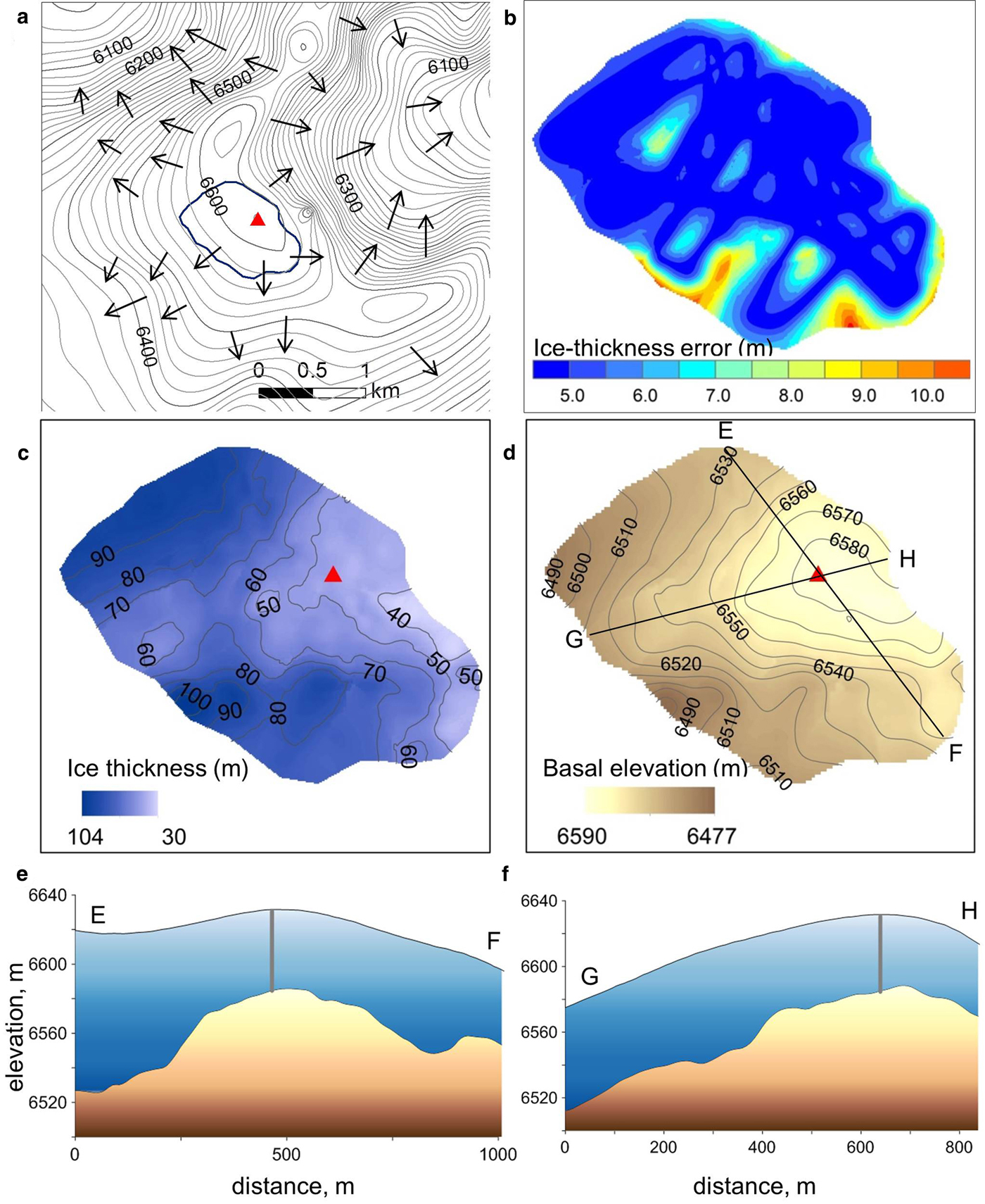
Ice thicknesses and basal topography of the summit region around the drill sites are shown in Fig. 7. GPR profiles located 15–20 m away from the GS drilling site reveal ice/bed interface reflections at a depth of 48.5 ± 4.53 m (Fig. 7), which agree well with the depths of three boreholes (50.72, 51.38 and 50.86 m) drilled at the summit. Such a good agreement between GPR and borehole depths confirms our approach to RWV calculations at the GS site. The average measured ice thickness for the GS site was 63 ± 4.61 m, with a maximum measurement of 97.64 ± 4.84 m. However, the use of 0.168 m ns−1 RWV for the same GPR data at the GS site results in larger uncertainty, leading to an ice thickness underestimation of 11%. GRP results show uniform accumulation distribution and smooth, continuous, undisturbed internal glacier structure in the vicinity of the drilling site. The surface and basal topography confirms that the GS drilling site is located at the ice dome where the horizontal ice velocity is negligible.
(a) Surface topography, glacier ice drainage basins (black lines) and ice flow direction (arrows), GPR measurement GS site outline (blue line). (b) Total ice thickness error map for the GS site. (c) Ice thickness and (d) basal topography on the GS. Surface and basal topography at cross sections (c) E-F and (d) G-H are shown.
These findings were compared with the results from the first GPR survey on the Guliya ice cap in May 1991 (Thompson and others, Reference Thompson1995). Point measurements revealed a similar u-shaped valley; however, the number of measurements was limited and it was impossible to make any reliable estimates of the actual ice thickness distribution. It has to be noted that the comparison is only qualitative and should not be used for verification as the accuracy of georeferencing in 1991 cannot be estimated. Nevertheless, the direct comparison between all the measured points available from the 1991 field notes and the published data in Thompson and others (Reference Thompson1995) show a good agreement for the GP site. Measurements made in 1991 at seven points located within the area surveyed in 2015 on average show a 12 m lower ice thickness with a std dev. of 21 m. The only available point measurements for the GS site showed an ice thickness of 103 m, which is roughly twice as much as revealed by the drilling and GPR survey of 2015. This difference can be explained partly by the lack of georeferencing, but most likely is due to misinterpretation of the 1991 radar data. Only minor elevation and hence ice thickness changes are detected for the GS site between 2000 and 2015 and there is no reason to expect a significant ice thickness decrease between 1991 and 2000. Thus, it is possible that the multiple reflections (echoes) in the 1991 record were interpreted as real bedrock reflections, leading to an overestimation of the depth by a factor of two.
Results of the DEM differencing are presented in Fig. 8. The Alakesayi glacier to the north of Guliya was considered by Yasuda and Furuya (Reference Yasuda and Furuya2015) to be a possible surging glacier, and the most noticeable feature of the DEM differencing results is the significant surface elevation change, which is due to a surge event (Fig. 8a, b). The WorldView-1 imagery of the Alakesayi glacier used for HMA-8 DEM was acquired in August 2015. Since 2000 the surface elevation had decreased by 40 m at the upper part of the glacier and increased by 60–80 m at the tongue, which indicated a fast glacier advance as registered by satellite imagery. The active phase of the surge event took place from 2015 to 2017 when the glacier advanced by 1.2 km. However, a detailed investigation of this surge lies outside the scope of our study. In contrast, the Guliya ice cap does not reveal any signs of surging in the past, and is categorized as non-surge type glacier (Yasuda and Furuya, Reference Yasuda and Furuya2015). Over the past 15 years since the SRTM mission, an overall rise of the Guliya glacier surface was observed (Fig. 8a, c). Surface elevation has increased by 8.64 ± 3.62 m at the GS drilling site and by 4.93 ± 3.62 m at the GP site. An average density of 0.47 g cm−3 was measured for the upper 9 m of firn in the GS ice cores, while at the GP site average density is 0.85 g cm−3. This gives the specific annual mass balance of 0.270 ± 0.11 and 0.279 ± 0.11 m w.e. a−1 at the GS and GP sites, respectively in 2000–2015. Essentially similar results within the range of uncertainty were obtained for the 1991–2015 period (GS: 0.106 m w.e. a−1; GP: 0.222 m w.e. a−1) by direct comparison of ice cores drilled in the early 1990s with the 2015 GP and GS cores (Thompson and others, Reference Thompson2018). The average surface increase over the entire Guliya glacier covered by the HMA-8 m DEM was 1.60 ± 3.62 m, or 0.09 ± 0.11 m w.e. a−1 in 2000–2015 period. Our results correspond well with recent studies of the glacier changes in West Kunlun glaciers and confirm the overall mass gain since the beginning of 21st century. Based on a comparison of ICESat repeated tracks, Ke and others (Reference Ke, Ding and Song2015) concluded that the surface of the Guliya ice cap was rising in the accumulation zone at an average rate of 0.3 ± 0.1 m a−1 during the 2003–08 period. Lin and others (Reference Lin, Li, Cuo, Hooper and Ye2017) estimated a mass balance on Guliya of 0.230 m w.e. a−1 from 2000 to 2014 based on SRTM-X-band DEM and bistatic TerraSAR-X/TanDEM-X comparison. Slightly lower mass balance values obtained in our study may be explained by the HMA-8 m DEM data gaps which constitute approximately one-half of the glacier area.
(a) Surface elevation changes from 2000 to 2015 obtained as SRTM-X and HMA-8 DEM differencing. Area and length changes of the Alakesayi glacier in 2015–17 are shown. (b) and (c) Elevation changes for selected profiles at Alakesayi (A-B) and Guliya glacier (C-D). Areas not covered by the elevation change data represent gaps in HMA-8 DEM. Background image is a Sentinel-2A image from 08 August 2017.
5. CONCLUSIONS
We have presented a new and valuable ice thickness dataset collected in 2015 on the Guliya ice cap. GPR ice thickness data were compared with the borehole depths and ice core stratigraphy. The constant RWV of 0.168 m ns−1 provides the best match to borehole depth where firn is absent. The ice thickness measured near the GP drilling site differs by <4 m from the borehole depth (309.73 m). For the GS where a firn layer is present, a calibration of the RWV using the density profile was used. Measured ice thickness near the GS site of 48.5 ± 4.53 m agrees well with depths of the boreholes (50.72, 51.38 and 50.86 m).
The EBK used for the interpolation of the GPR data and interpolation uncertainty estimation is a useful tool for GPR measurements. It solves the problem of cross validation and underestimation of the interpolation error in an automated way by data subsetting and estimating semivariogram model errors. The major sources of interpolation uncertainty are the interpolation error between widely separated measurement profiles and the interpolation between profiles over areas of abrupt changes of ice thickness.
GPR measurements revealed complex basal topography in the vicinity of the GP drill site (Fig. 5). The average ice thickness on the plateau was 228.76 ± 11.69 m, with a maximum thickness of 371.12 ± 13.02 m. Radar data obtained using the 20 MHz frequency antennas on the GP did not reveal any continuous internal reflections; however, the low frequency enabled ice/bed interface detection in the deeper parts (Fig. 4). Surface topography and ice thickness distribution suggest low horizontal ice flux on the GP.
The average measured ice thickness on the GS site was 63 ± 4.61 m, and the maximum was 97.64 ± 4.84 m (Fig. 7). Uninterrupted internal reflections were registered at the GS drilling site by the 40 MHz frequency GPR (Fig. 6). They were interpreted as isochrone layers that resulted from firn density variations.
The Guliya ice cap gained mass from 2000 to 2015. The surface elevation increased by 8.64 ± 3.62 m (0.270 ± 0.11 m w.e. a−1) at the GS drilling site and by 4.93 ± 3.62 m (0.279 ± 0.11 m w.e. a−1) at the GP site (Fig. 8). The average surface elevation increase over Guliya that was covered by the HMA-8 m DEM was 1.60 ± 3.62 m or 0.09 ± 0.11 m w.e. a−1.
Our data complement the world's ice thickness dataset and can be used for further improvements of ice thickness models for ice caps and are archived at https://www.ncdc.noaa.gov/paleo/study/25130.
ACKNOWLEDGEMENTS
This research was accomplished as part of collaborative expedition between The Ohio State University's Byrd Polar and Climate Research Center (BPCRC) and the Institute of Tibetan Plateau Research (ITP) of the Chinese Academy of Sciences funded by the National Science foundation Paleoclimate Program award #1502919 and the Chinese Academy of Sciences, respectively. We thank all the field and laboratory team members from the Institute of Tibetan Plateau Research led by Prof. Tandong Yao, and from the Ohio State University's Byrd Polar and Climate Research Center for their invaluable contribution in supporting the 2015 Guliya field project. A special thanks to Dr Emilie Beaudon (BPCRC) for making the density and stratigraphy measurements shown in Fig. 3. This is Byrd Polar and Climate Research Center contribution number 1566.


 Open access