


1. Introduction
Global warming has resulted in notable environmental changes in the cryosphere. The rate of temperature increase in the Arctic has been four times greater than the global average since 1979 (Rantanen and others, Reference Rantanen2022). This phenomenon has been widely documented in observational and modeling studies as ‘Arctic Amplification’ (e.g. Manabe and Wetherald, Reference Manabe and Wetherald1975; Johannessen and others, Reference Johannessen2004; Pithan and Mauritsen, Reference Pithan and Mauritsen2014). One cause of Arctic Amplification is a positive ‘ice-albedo feedback’ (Budyko, Reference Budyko1969; Sellers, Reference Sellers1969; Manabe and Wetherald, Reference Manabe and Wetherald1975), which amplifies the rate of temperature increase. Warming leads to snow metamorphosis, which further decreases the albedo and accelerates melting. Rapid warming in the Arctic has accelerated the mass loss of the Greenland Ice Sheet and its peripheral glaciers (Hanna and others, Reference Hanna2013; The IMBIE Team, 2020). Warming in the Arctic not only causes mass loss but also a reduction in sea ice extent (Cavalieri and Parkinson, Reference Cavalieri and Parkinson2012; Fox-Kemper and others, Reference Fox-Kemper and Masson-Delmotte2021), and an increase in river runoff (Feng and others, Reference Feng, Gleason, Lin, Yang, Pan and Ishitsuka2021). These changes indicate a shift in the hydrological circulation system (van Tiel and others, Reference van Tiel2024). In particular, the supply of fresh water resulting from the increased runoff of land snow and ice (Ohmura, Reference Ohmura2011; van den Broeke and others, Reference van den Broeke2016; Hugonnet and others, Reference Hugonnet2021) has a significant impact on various climate systems, such as atmospheric and oceanic circulations (Callaghan and others, Reference Callaghan, Johansson, Key, Prowse, Ananicheva and Klepikov2011; Prowse and others, Reference Prowse2015). Consequently, it is of utmost importance to gain a comprehensive understanding of the present Arctic environment and make accurate predictions regarding its future.
Accelerated glacier mass loss is particularly pronounced in relatively low-elevation areas, such as the coastal and peripheral glaciers in Greenland (Noël and others, Reference Noël2017; Khan and others, Reference Khan, Colgan, Neumann and van den Broeke2022) and the northwest region of Greenland (Mouginot and others, Reference Mouginot2019; Niwano and others, Reference Niwano, Box, Wehrlé, Vandecrux, Colgan and Cappelen2021). Studies have been conducted in the Qaanaaq region in northwest Greenland to understand the current conditions of environmental changes (Sugiyama and others, Reference Sugiyama, Sakakibara, Matsuno, Yamaguchi, Matoba and Aoki2014) and evaluate the effects of environmental changes in Greenland (Kondo and others, Reference Kondo, Sugiyama and Fukumoto2021; Niwano and others, Reference Niwano, Box, Wehrlé, Vandecrux, Colgan and Cappelen2021). Tsutaki and others (Reference Tsutaki, Sugiyama, Sakakibara, Aoki and Niwano2017) and Sugiyama and others (Reference Sugiyama2021) presented the surface mass balance (SMB) of the Qaanaaq Glacier using stake observations. The studies indicated that the annual SMB near the 950 m elevation zone for the period 2012/13–2018/19 varied between −0.5 and +0.6 m w.e. a−1. In addition, the equilibrium line altitude (ELA), which is defined as the line where the annual SMB of the Qaanaaq Glacier is zero (Cogley and others, Reference Cogley2011), is situated within an elevation zone between 700 and 1000 m a.s.l.
Since the late 1970s, the ELA has risen on most of the world’s glaciers, with a maximum rate of 9.5 m/year (Ohmura and Boettcher, Reference Ohmura and Boettcher2022). Monitoring the mass change over several years, which is highly variable from year to year at the ELA, is a valuable indicator for assessing glacial mass loss (Ohmura and Funk, Reference Ohmura and Funk1992; Braithwaite, Reference Braithwaite2015). Although most methods for estimating the ELA are based on satellite remote sensing (e.g. Racoviteanu and other, Reference Racoviteanu, Rittger and Armstrong2019; Rastner and others, Reference Rastner2019) and climate data, particularly summer temperatures and winter precipitation (e.g. Ohmura and Boettcher, Reference Ohmura and Boettcher2018; Nesje, Reference Nesje2023), it is difficult to identify the factors that cause variations in the ELA using these methods. Therefore, a systematic understanding of which meteorological factors control the annual mass balance and which factors govern the ELA has not yet been achieved. From this perspective, understanding the surface energy balance (SEB), which represents the primary energy exchange system between the atmosphere and the surface, is crucial for understanding the environmental conditions conducive to the SMB persistence of snow and ice. Information on the SEB is essential for calculating the amount of surface melt (Niwano and others, Reference Niwano2015) and evaluating the effect of sublimation on glacier or ice sheet SMB (Stigter and others, Reference Stigter2018; Dietrich and others, Reference Dietrich, Steen-Larsen, Wahl, Faber and Fettweis2024).
The fact that the annual ELA varies significantly from year to year means that the area around the ELA is either exposed or not exposed to the ice surface. In other words, the albedo varies significantly from year to year (Ryan and others, Reference Ryan2019). Surface albedo is one of the most important factors controlling the SEB, and a decrease in albedo provides a large amount of energy input, resulting in a significant decrease in the SMB. In addition, changes in albedo alter the radiative forcing of clouds (Ramanathan and others, Reference Ramanathan1989). When clouds form over surfaces with low albedo, the radiative forcing can be negative, resulting in a cooling effect (Wang and others, Reference Wang, Zender and van As2018). In Greenland, surface melting has also been reported to be accelerated by cloud formation (Niwano and others, Reference Niwano, Hashimoto and Aoki2019).
In this context, the SEB near the ELA is controlled by intense changes in the surface (albedo) and atmospheric (clouds and radiation) conditions, making it necessary to analyze them in combination to understand the mechanism of glacier ELA movement. Previous studies conducted in Greenland have tended to focus on ablation areas (e.g. Fausto and others, Reference Fausto, van As, Box, Colgan and Langen2016; Abermann and others, Reference Abermann, van As, Wacker, Langley, Machguth and Fausto2019). There are few studies discussing the SMB based on in situ meteorological observation data on polar glaciers on the periphery of ice sheets (e.g. Reijmer and van den Broeke, Reference Reijmer and van den Broeke2003; van den Broeke and others, Reference van den Broeke, Reijmer and van de Wal2004b), and few studies near the ELA have been presented. In this study, we focused on interannual variations over a decade in the SEB and SMB near the ELA of the Qaanaaq Ice Cap in northwest Greenland and the factors controlling these variations (particularly, albedo, clouds and radiation). We quantitatively elucidated the mechanisms of annual variation in the SEB and SMB.
2. Data and methods
2.1. Site description of SIGMA-B and AWS instrumentation
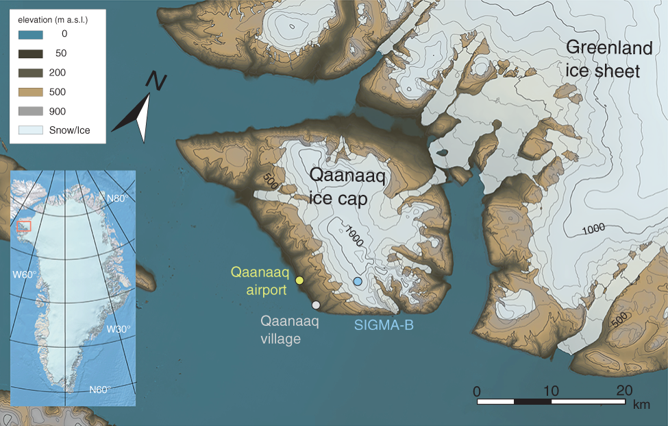
The Qaanaaq Ice Cap is a peripheral ice cap on the Greenland Ice Sheet with an elevation range of 30–1110 m a.s.l. (Sugiyama and others, Reference Sugiyama, Sakakibara, Matsuno, Yamaguchi, Matoba and Aoki2014). The Qaanaaq Ice Cap is located in the northwestern Greenland coastal area (Fig. 1).
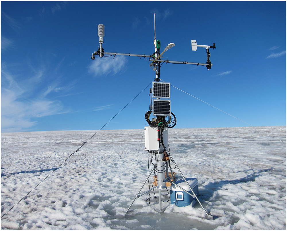
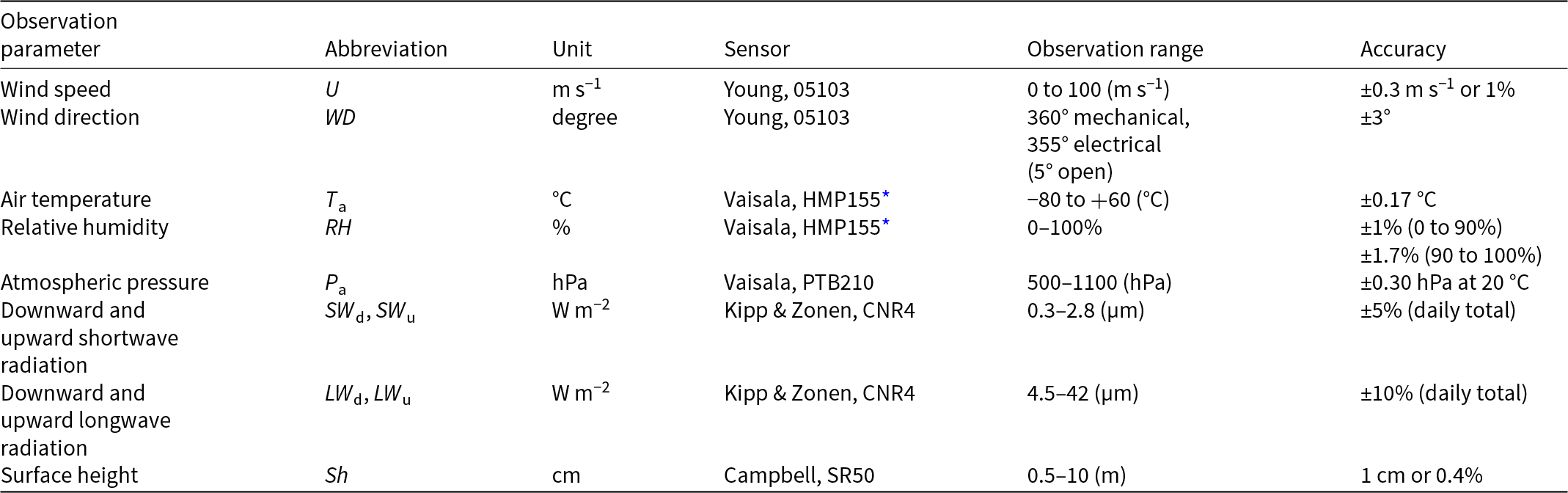
In July 2012, an Automatic Weather Station (AWS) was established at the SIGMA-B site (77.518°N, 69.062°W; elevation 944 m a.s.l.) on the mid-slope of the Qaanaaq Ice Cap (Aoki and others, Reference Aoki, Matoba, Uetake, Takeuchi and Motoyama2014) (Figs. 1 and 2). The objective of this installation was to monitor meteorological and glaciological conditions around the ELA. Table 1 lists the observed parameters and sensor specifications, including air temperature, relative humidity, wind speed and direction, atmospheric pressure, surface height, downward and upward shortwave radiation and downward and upward longwave radiation. Hourly data were derived by averaging the 1-min sampled data, and the surface height was recorded at hourly intervals. Further details regarding the observation site and AWS instrumentation can be found in studies by Aoki and others (Reference Aoki, Matoba, Uetake, Takeuchi and Motoyama2014) and Nishimura and others (Reference Nishimura2023). This study analyzed AWS data collected over a 10-year period from 20 July 2012 to 31 August 2022, defining a mass balance year as the period from 1 September to 31 August.
Map of Greenland (bottom left) and the location of the SIGMA-B site (main map). The contour intervals of the thick and thin lines in the main map are set to 500 and 100 m a.s.l., respectively.

Overview of the AWS system at the SIGMA-B site in July 2012.

Meteorological observation parameters and sensor specifications provided by Nishimura and others (Reference Nishimura2023).

* Protected from direct solar irradiance by a naturally aspirated 14-plate Gill radiation shield (20 July 2012–10 July 2022) and a forced-ventilated radiation shield (10 July 2022–).
2.2. Data processing and analysis
2.2.1. Data processing
Quality-controlled AWS data (Nishimura and others, Reference Nishimura2023) were used, and SEB and SMB were calculated at hourly time steps. This study used surface height data as a 19 h running mean to smooth out minor fluctuations due to observation errors resulting from the surrounding atmospheric and near-surface environment, and to clarify the trend of increase or decrease in the surface height.
Furthermore, the AWS data may contain observation biases due to heating of the naturally ventilated air temperature and humidity sensors by solar radiation and underestimation of the relative humidity data recorded in a freezing environment. This study employed the methodology proposed by Nakamura and Mahrt (Reference Nakamura and Mahrt2005) and Huwald and others (Reference Huwald, Higgins, Boldi, Bou-Zeid, Lehning and Parlange2009) to correct the air temperature to account for the shelter heating effect.
 \begin{equation}{T_{{\text{cor}}}} = {T_{\text{a}}} - \frac{{S{W_{\text{u}}}}}{{{\rho _{\text{a}}}{{\text{C}}_{\text{p}}}{T_{\text{a}}}U}},\end{equation}
with T cor denoting the corrected air temperature using upward shortwave radiation (SW u), air density (ρ a), specific heat capacity of air (Cp), wind speed (U) and observed air temperature (T a).
The relative humidity (RH obs) data might be underestimated under below-freezing conditions owing to the differing saturated vapor pressures of water and ice (Anderson, Reference Anderson1994), mainly because RH obs was calculated using a water-saturated vapor pressure based on sensor specifications. To address this issue, the temperature bins below −20°C, where underestimation is expected to be most pronounced, were divided into 0.5°C intervals. Then, the top 5% of the relative humidity (RH max) in each bin was calculated. The corrected relative humidity (RH cor) was rescaled using RH max as follows:
 \begin{equation}R{H_{{\text{cor}}}} = \frac{{R{H_{{\text{obs}}}}}}{{R{H_{{\text{max}}\left( {{T_a}} \right)}}}}.\end{equation}
2.2.2. Surface energy balance analysis
The SEB and radiative fluxes were calculated using the following equations:
 \begin{equation}\frac{{{\text{d}}U}}{{{\text{d}}t}} = S{W_{\text{d}}} - S{W_{\text{u}}} + L{W_{\text{d}}} - L{W_{\text{u}}} + H + \iota E + {Q_{\text{R}}} + {Q_{\text{S}}},\end{equation}
 \begin{equation}S{W_{{\text{net}}}} = S{W_{\text{d}}} - S{W_{\text{u}}} = \left( {1 - \alpha } \right)S{W_{\text{d}}},\end{equation}
 \begin{equation}L{W_{{\text{net}}}} = L{W_{\text{d}}} - L{W_{\text{u}}} = \varepsilon L{W_{\text{d}}} - \varepsilon \sigma {T_{\text{s}}}^4,\end{equation}
 \begin{equation}{R_{{\text{net}}}} = S{W_{{\text{net}}}} + L{W_{{\text{net}}}},\end{equation}
 \begin{equation}{R_{{\text{abs}}}} = S{W_{{\text{net}}}} + \varepsilon L{W_{\text{d}}},\end{equation}
where dU/dt denotes the rate of exchange of internal energy of the surface layer (Lackner and others, Reference Lackner2022). In this study, the surface layer was defined as the layer from 0 to 1 cm below the surface. Downward and upward shortwave and longwave radiation (SW d, SW u, LW d and LW u, respectively) were observed. The net shortwave and longwave (SW net and LW net, respectively), surface albedo (α) and surface temperature (T s) were calculated using the radiation components and Stefan–Boltzmann relation, with the Stefan–Boltzmann constant σ = 5.67 × 10⁻⁸ W m−2 K−4 and emissivity of snow/ice ɛ = 0.98 (Jordan and others, Reference Jordan, Albert, Brun and Brun2008). To evaluate the validity of SEB analysis (Section 3.1), we calculated the modeled surface temperature under the assumption that the SEB had reached a steady state (dU/dt = 0). This was obtained by solving the SEB equation (Eq. 3), with the surface temperature as the unknown variable. It was assumed that all the shortwave radiant fluxes were absorbed by the surface layer. The radiant flux absorbed by the surface (R abs; Kondo and Yamazaki, Reference Kondo and Yamazaki1990) is defined as the sum of SW net and downward longwave radiation absorbed by the surface (ɛLW d). R abs is an important term in the SEB equation because it does not depend on the surface temperature; that is, it forces the SEB. H and lE denote the sensible and latent heat fluxes, respectively. Q R denotes the rainfall energy flux, and Q S denotes the subsurface heat flux through the boundary at a depth of 1 cm. In this study, all energy fluxes directed toward the surface were defined as positive.
H and lE were calculated using the bulk aerodynamic method as follows:
 \begin{equation}H = {\rho _a}\,{{\text{C}}_p}\,{C_H}\,U\,\left( {{\theta _a} - {\theta _s}} \right),\end{equation}
 \begin{equation}lE = {\rho _a}\,l\,{C_E}\,U\,\left( {{q_a} - {q_s}} \right),\end{equation}
where C H and C E denote the bulk exchange coefficients for the sensible and latent heat fluxes, respectively; ρ a [kg m−3] denotes the moist air density; C p (= 1.005 kJ K−1 kg−1) denotes the atmospheric specific heat at constant pressure; l [J kg−1] denotes the latent heat of evaporation or sublimation; θ a and θ s [K] denote the potential temperatures of the surface atmosphere and the surface, respectively; q a and q s [g kg−1] denote the atmospheric and surface specific humidity, respectively. In this study, the surface conditions were assumed to be saturated.
The bulk coefficients (C H and C E) were calculated through an iterative procedure, considering the atmospheric stability as determined by the Monin–Obukhov stability length and a stability parameter. The surface roughness lengths for wind speed, air temperature and relative humidity (z 0v, z 0t and z 0e) used to derive the C H and C E were calculated following the procedure described by Andreas (Reference Andreas1987). The z 0v parameter was defined as a constant value for each surface condition and classified according to the observed T s and surface albedo. The values for z 0v,d (dry snow), z 0v,w (wet snow) and z 0v,i (ice) were 0.12 × 10⁻³ [m], 1.3 × 10⁻³ [m] and 3.2 × 10⁻³ [m], respectively (Greuell and Konzelmann, Reference Greuell and Konzelmann1994).
The rainfall energy flux (Q R) is the energy flux advected by raindrops and is calculated as follows:
 \begin{equation}{Q_R} = {P_{rain}}\,{\rho _w}\,{C_w}\,\left( {{T_w} - {T_s}} \right),\end{equation}
where P rain denotes the rainfall intensity [m s−1]; ρ w (= 1000 kg m−3) and Cw (= 4217 J kg−1 K−1) denote the density and specific heat of water, respectively; and T w [K] denotes the wet-bulb temperature. P rain was derived from the analyzed value at the nearest-neighbor grid point of the polar regional climate NHM-SMAP model (Niwano and others, Reference Niwano2018, Reference Niwano, Box, Wehrlé, Vandecrux, Colgan and Cappelen2021) because precipitation observations were not performed at the SIGMA-B site.
This study also used Q s values derived using the NHM-SMAP model. Q s can vary spatially depending on near-surface atmospheric conditions and the resulting snow physical conditions. At the SIGMA-B site, the near-surface snow conditions often become isothermal due to frequent surface melt (July averaged T s = −0.6°C; see Table 2). Therefore, the Q s values at the SIGMA-B site from the NHM-SMAP model were assumed to be realistic. However, when applying the SEB model presented in this paper to other sites where the absolute subsurface conductive heat flux can be as high as 6.1 W m−2 (Abermann and others, Reference Abermann, van As, Wacker, Langley, Machguth and Fausto2019), it is necessary to consider the subsurface processes—such as heat conduction, meltwater percolation and refreezing.
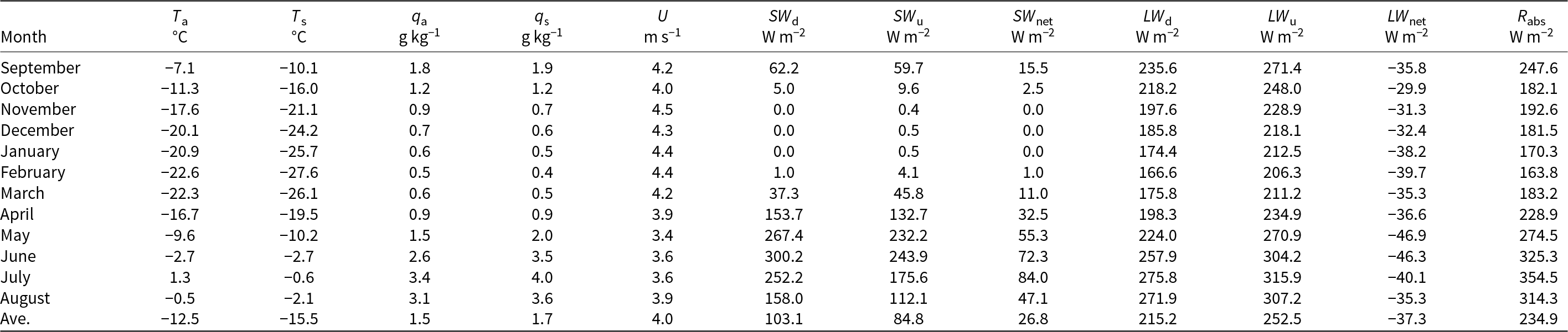
Monthly averages of meteorological parameters from August 2012 to August 2022.

2.2.3. Surface mass balance analysis
The SMB is defined as follows:
 \begin{equation}SMB = P + RU + S{U_{\text{s}}} + E{R_{{\text{ds}}}},\end{equation}
 \begin{equation}RU = M + RFA,\end{equation}
where P represents precipitation, including snowfall (P snow [m w.e. s−1]) and rainfall (P rain); RU denotes meltwater runoff, which is defined as the difference between the amount of surface melt (M) and the refreezing amount within the snow layer (RFA); SU s denotes the water vapor flux due to sublimation, deposition, evaporation and condensation; and ER ds denotes the negative snow mass flux triggered by wind erosion and snow drift. The sign of each variable is considered positive for mass gain and negative for mass loss. This study employed a surface model that did not incorporate water movement or storage in snowpacks. Consequently, the RFA was estimated based on the change in ice surface height for each year (Table S2 and Fig. S1). The bare-ice surface height was identified using the observed surface height when the albedo fell below the ice threshold (0.565; Wehrlé and others, Reference Wehrlé, Box, Niwano, Anesio and Fausto2021). The RFA quantity was then calculated as the difference in surface height between the years when the bare-ice surface was exposed, providing the thickness of the superimposed ice formed during that period. This value was then multiplied by the ice density (917 kg m−3) to calculate the amount of water that refroze below the surface. The negative RFA results (Fig. S1) indicate that the ice surface declined during that year, i.e. the amount of ice was lost. However, because the ice surface was not observed in some years, the RFA values were estimated by interpolating the calculated yearly RFA values for the years in which ice surface was observed. Therefore, the amount of refreezing in the years when the ice surface was not observed remains uncertain.
P snow was calculated using the hourly positive change in surface height (sh), written as follows:
 \begin{equation}{P_{{\text{snow}}}} = \left( {s{h_{\text{i}}} - s{h_{{\text{i}} - 1}}} \right)\,{\rho _{{\text{s}},{\text{ new}}}},\end{equation}
where i represents the time index and ρ s,new denotes the density of precipitation in the form of snow calculated using the methodology proposed by Jordan and others (Reference Jordan, Andreas and Makshtas1999).
M was calculated using two methods: the surface height method (SHM), which uses the difference in hourly surface height data, and the SEB model. The difference between the two SMBs (SMB SHM and SMB SEB) results solely from the melt components (M SHM and M SEB) because all other terms in the SMB equation are identical.
Using the SHM (M SHM) when T s = 0°C and the sh change is negative, the melt amount is calculated as follows:
 \begin{equation}{M_{{\text{SHM}}}} = \left( {s{h_{\text{i}}} - s{h_{{\text{i}} - 1}}} \right)\,{\rho _{{\text{surface}}}},\end{equation}
where ρ surface [kg m−3] denotes the surface snow/ice density. The surface density was considered to be constant for each surface condition. The surface conditions were determined using the surface albedo (Wehrlé and others, Reference Wehrlé, Box, Niwano, Anesio and Fausto2021) as follows:
 \begin{align}
&{\rho _{surface}} \nonumber\\
&= \left\{ \begin{array}{*{20}{c}}
570\,\,kg\,{m^{ - 3}}for\,albedo \geqslant 0.565\,\left( {{\text{surface condition}}:{\text{ wet snow or firn}}} \right) \\
917\,kg\,{m^{ - 3}}\,for\,albedo \lt 0.565\,\left( {{\text{surface condition}}:{\text{ ice}}} \right)
\end{array} \right.\!\!\!\!.\end{align}
\begin{align}
&{\rho _{surface}} \nonumber\\
&= \left\{ \begin{array}{*{20}{c}}
570\,\,kg\,{m^{ - 3}}for\,albedo \geqslant 0.565\,\left( {{\text{surface condition}}:{\text{ wet snow or firn}}} \right) \\
917\,kg\,{m^{ - 3}}\,for\,albedo \lt 0.565\,\left( {{\text{surface condition}}:{\text{ ice}}} \right)
\end{array} \right.\!\!\!\!.\end{align}The value of 570 kg m–3, which was employed as the wet snow or firn density in this study, was higher than the commonly used values (e.g. wet snow: 422 kg m–3, DeWalle and Rango, Reference DeWalle and Rango2008; firn: 510–700 kg m–3; Huss, Reference Huss2013). Determining whether the surface was compacted firn or wet snow was difficult based on the meteorological data. Thus, the exact density remained uncertain. The density higher value used in this study was determined by sensitivity tests and an analysis of the results of the SEB and SHM methods (see Appendix B). Consequently, a representative surface density that included both wet snow and firn conditions was used.
The amount of surface melt determined using the results of the SEB model (M SEB) was calculated using the following equation:
 \begin{equation}{M_{{\text{SEB}}}} = \frac{{{Q_{\text{M}}}}}{{{\rho _{\text{w}}}\,{l_{{\text{f}},{\text{ i}}}}}},\end{equation}
where l f, i (334 × 103 J kg−1) denotes the latent heat of fusion required for melting ice at 273.15 K, and Q M denotes the energy available for surface melt. When T s = 0 °C and dU/dt > 0, dU/dt is equal to Q M.
SU s, which include the four processes of sublimation, deposition, evaporation and condensation, was calculated using the latent heat flux and surface temperature. The latent heat associated with a change in the state of water was estimated using the following equation:
 \begin{equation}S{U_{\text{s}}} = \frac{{{{\iota }}E}}{{{l_{\text{v}}}\,{\rho _{\text{w}}}}},\end{equation}
where l v denotes the latent heat for water or ice.
ER ds was calculated using an equation similar to Eq. (14). The difference from the determination of M SHM is that ER ds was calculated exclusively when the surface was snow (classified according to surface albedo), the surface temperature was below 0°C and the friction velocity ( ${u_*}$) was greater than a threshold value determined based on the methodology reported by Gallée and others (Reference Gallée, Guyomarc’h and Brun2001). The surface density was calculated from the snow density of the uppermost layer (surface) in the snow densification calculation (described below), as surface conditions cannot be classified using surface albedo in winter owing to the absence of shortwave radiation.
In the calculations of P snow, M SHM and ER ds, the change in surface height was determined by accounting for the influence of snow densification resulting from the weight of the overlying snowpack. The degree of surface degradation was calculated using the following densification equation:
 \begin{equation}\frac{1}{{{\rho _s}}}\frac{{\partial {\rho _s}}}{{\partial t}} = \frac{\sigma }{\eta },\end{equation}
where ρ s denotes the snow density [kg m−3], σ denotes the overburden pressure [Pa] and η denotes the compression viscosity coefficient of snow [Pa sec]. η was calculated according to the procedures of Bader and Weilenmann (Reference Bader and Weilenmann1992) and Morris and others (Reference Morris, Bader and Weilenmann1997). The initial value for the snow density was determined based on the new snow density parametrization proposed by Jordan and others (Reference Jordan, Andreas and Makshtas1999), and the surface temperature was used as the initial value for the snow temperature. However, the model used in this study did not account for temporal change in snow temperature within the snowpack because it did not include the calculation of internal energy exchange within the snowpack or the vertical temperature profile.
2.2.4. Parameterization of cloudiness
Longwave-equivalent cloudiness (N ε) was used an indicator of cloud regime and climatology. This variable was proposed and implemented by van den Broeke and others (Reference van den Broeke, Reijmer and van de Wal2004a) and Conway and others (Reference Conway, Cullen, Spronken-Smith and Fitzsimons2015). N ε was calculated as follows:
 \begin{equation}{N_{{\varepsilon }}} = \frac{{{\varepsilon _{{\text{eff}}}} - {\varepsilon _{{\text{cs}}}}}}{{{\varepsilon _{{\text{ov}}}} - {\varepsilon _{{\text{cs}}}}}},\end{equation}
 \begin{equation}{\varepsilon _{{\text{eff}}}} = \frac{{L{W_{\text{d}}}}}{{\sigma \left( {{T_{\text{a}}} + {T_{{\text{abs}}}}} \right)}},\end{equation}
 \begin{equation}{\varepsilon _{cs}} = {\varepsilon _{dry}} + \,{C_1}\,{\left( {\frac{{{e_a}}}{{{T_a} + {T_{abs}}}}} \right)^{\frac{1}{{{C_2}}}}},\end{equation}
where ε eff, ε cs and ε ov [–] denote the effective, clear-sky and overcast atmospheric emissivities, respectively; T abs (273.15 K) denotes the absolute temperature. The dry atmospheric emissivity (ε dry) was set to 0.23 (Konzelmann and others, Reference Konzelmann, van de Wal, Greuell, Bintanja, Henneken and Abe-Ouchi1994). The constants C1 (= 0.603) and C2 (= 11) were determined based on a method proposed by Konzelmann and others (Reference Konzelmann, van de Wal, Greuell, Bintanja, Henneken and Abe-Ouchi1994), using the monthly mean observed water vapor pressure, air temperature and atmospheric emissivity at the SIGMA-B site. The calculated distribution of N ε was normalized by setting the thresholds at the upper 98th percentile (1.2) and the lower 2nd percentile (−1.0). The dataset was then rescaled using these thresholds so that the normalized values ranged from 0 to 1, with 0 indicating clear-sky conditions and 1 indicating overcast-sky conditions.
3. Results
3.1. Evaluation of surface energy and mass balance models
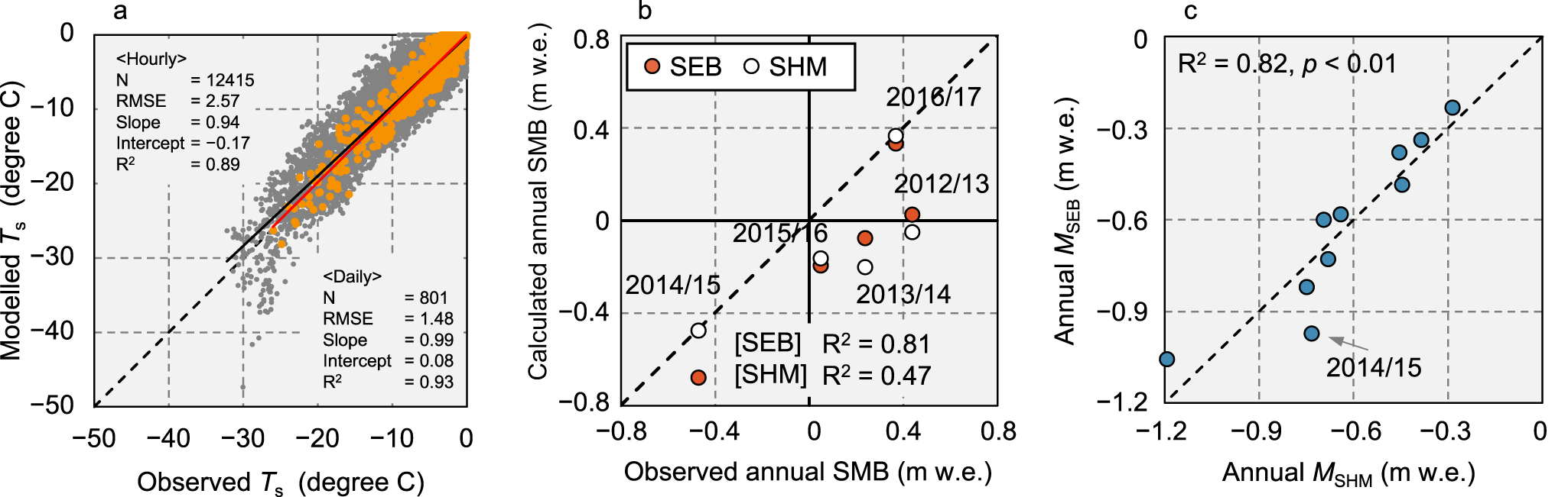
To evaluate the validity of the SEB and SMB analytical methods, the observed and calculated surface temperatures were compared (Fig. 3a). The root mean square errors (RMSEs) between the observed and modeled surface temperatures were 2.57°C and 1.48°C for hourly and daily data, respectively. The slopes of the regression lines were very close to unity, with biases of −0.17°C (hourly) and 0.08°C (daily). All statistical metrics indicated good reproducibility for the daily data.
Scatter plots of (a) observed and modeled surface temperatures (T s). The data plots for the hourly and daily time steps are colored gray and orange, respectively, and the regression lines are shown as solid black and red lines; (b) observed SMB from stake measurements reported by Tsutaki and others (Reference Tsutaki, Sugiyama, Sakakibara, Aoki and Niwano2017) and the calculated SMB SEB and SMB SHM; (c) annual surface mass balances (SMB) calculated using the surface energy balance analysis (SMB SEB) and surface height method (SMB SHM).

Huai and others (Reference Huai, van den Broeke and Reijmer2020) compared modeled and observed surface temperatures using the same method using AWS data observed in Greenland and reported RMSEs ranging from 1.1 to 1.6. Although the hourly results in this study exhibited larger errors than those reported by Huai and others (Reference Huai, van den Broeke and Reijmer2020), the daily results demonstrated sufficient accuracy. As shown in Fig. 3a, the calculated values occasionally underestimated the observations. These cases occurred primarily during or immediately after snowfall events and were likely attributed to uncertainties in the observed data. However, based on the regression results and coefficient of determination, the observed and calculated values were generally in good agreement.
In addition, Fig. 3b compares the SMB values calculated using the SEB model (SMB SEB) and SHM (SMB SHM) with the values obtained using stake measurements on the Qaanaaq Glacier between 2012 and 2016, as reported by Tsutaki and others (Reference Tsutaki, Sugiyama, Sakakibara, Aoki and Niwano2017). The annual SMB values shown in Fig. 3b were recalculated to match the measured stake observation periods reported by Tsutaki and others (Reference Tsutaki, Sugiyama, Sakakibara, Aoki and Niwano2017). Figure 3b shows that the coefficients of determination (R 2) between the observed and calculated SMB values were 0.81 (SEB) and 0.47 (SHM), and the RMSEs were 0.28 (SEB) and 0.31 (SHM) m w.e. The lowest error rates were obtained for the 2016/17 dataset (SEB: −0.04 m w.e.; SHM: 0.00 m w.e.). These results indicate that the SMB values calculated using the SEB method were more accurate than those calculated using the SHM. A comparison of the calculated annual melt amounts (M SEB and M SHM) in Fig. 3c shows that these M values were highly correlated (R 2 = 0.83, p < 0.01). Only the difference in the 2014/15 dataset (0.25 m w.e.) exceeded the two standard errors (SE = 0.11 m w.e.). Fettweis and others (Reference Fettweis2020) reported SMB RMSEs between model calculations and in situ observations in an intercomparison of regional climate models in Greenland. The RMSE for the PROMICE dataset (Machguth and others, Reference Machguth2016), which includes the SMB observations from the Greenland marginal ice caps, was reported to range from 0.48 to 0.89 m w.e. Although a direct comparison was not possible because the regional climate model, in situ dataset and observation periods differ, the RMSE obtained in this study is smaller than that reported by Fettweis and others (Reference Fettweis2020).
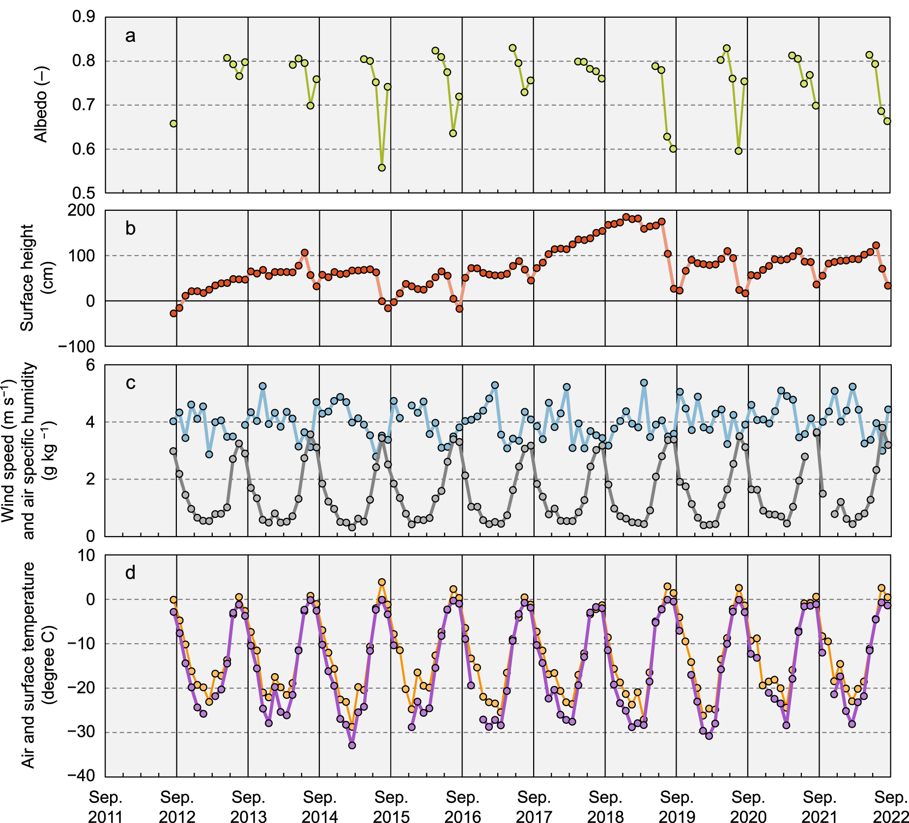
In July 2015, low albedo values were observed (monthly mean albedo = 0.56), as shown in Fig. 4a. Snow and firn layers accumulate during winter and subsequently experience melt. In this study, the surface density was treated as a constant depending on the surface state, even though, in practice, the surface snow density increases as snow metamorphoses. The difficulty in accurately determining the surface conditions and assigning the surface density may have contributed to the discrepancy observed between SMB SEB and SMB SHM in 2014/15.
Temporal variations in monthly mean (a) albedo, (b) surface height, (c) wind speed (blue) and air specific humidity (gray) and (d) air and surface temperatures (air: orange; surface: purple) between July 2012 and August 2022.

3.2. Climatological characteristics
This section describes the climatological characteristics of the major meteorological variables during the observational period. Figure 4 shows the monthly mean air and surface temperatures, air-specific humidity, wind speed, surface height and albedo. Table 2 lists the monthly decadal averages of several parameters from 2012 to 2022. In general, a positive monthly mean air temperature was observed in July, except in 2018 and 2021. The highest values were recorded in 2015 (+4.0°C) and 2019 (+3.0°C). A clear seasonal variation in air specific humidity was observed, with the lowest values occurring in winter and the highest values in summer. The maximum and minimum monthly averages for the 10 years were 3.4 g kg–1 in July and 0.5 g kg–1 in February. In contrast, the monthly mean wind speed did not exhibit a clear seasonal variation, ranging from 3.4 m s–1 in May to 4.5 m s–1 in November. The surface height increased between September and May and was significantly higher in 2019/20 (84.6 cm). In contrast, the increases were small in 2014/15 (14.3 cm) and 2018/19 (13.3 cm), particularly during the summer months (JJA: June, July and August; Fig. 4b). Significant surface degradation was also recorded during these years (2014/15: 144.3 cm, 2018/19: 83.9 cm).
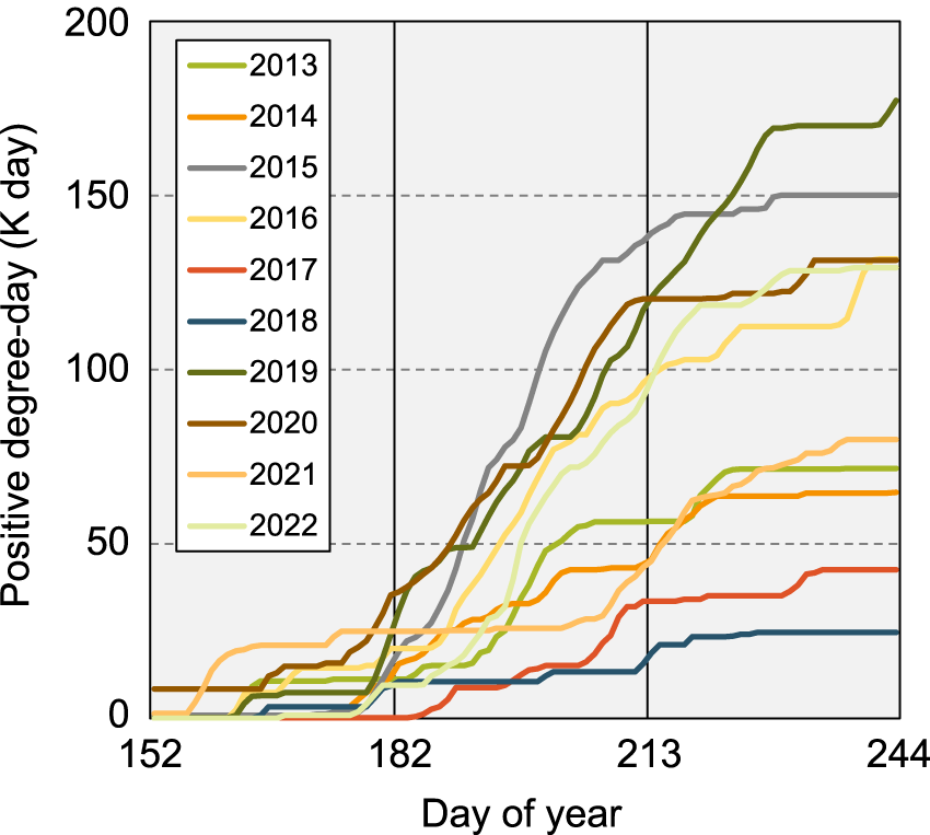
Figure 5 shows the temporal variation in cumulative positive degree days (PDDs) during all summers. High PDDs were recorded in 2014/15, 2015/16, 2018/19 and 2019/20 (150, 132, 177 and 131 K days, respectively). In addition, a significant decrease in albedo was observed during the summers of 2012, 2014/15, 2015/16, 2018/19 and 2019/20 (Fig. 4a), with the lowest value of 0.56 recorded in July 2015. Notably, the summer albedo was below 0.65 in summer in all other years mentioned above. The observed decreases in albedo and surface height were particularly pronounced in 2014/15 and 2018/19, which were years characterized by high air temperatures.
Temporal variation in cumulative positive degree days during summer (June–August) from 2013 to 2022.

3.3. Surface energy balance
3.3.1. General characteristics of surface energy balance
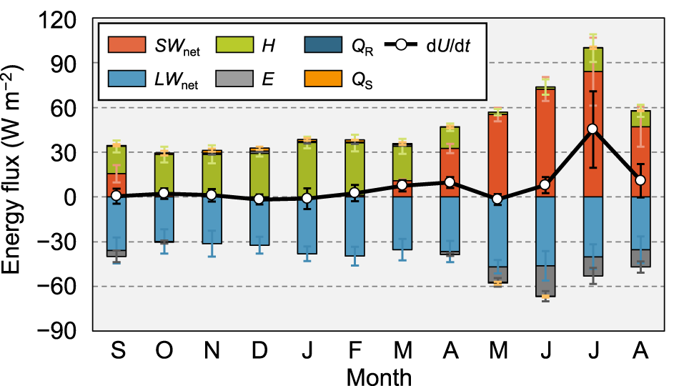
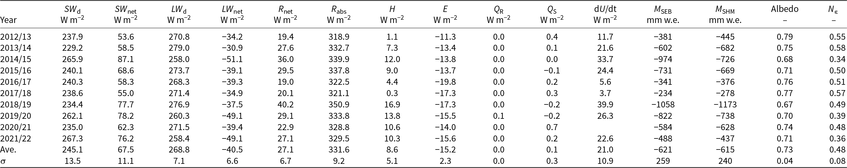
The 10-year averages of the radiation and SEB components are presented in Table 2 and Fig. 6. The summer averages of the main energy components (SW d, SW net, LW d, LW net, R net, R abs, H, E, Q R, Q S and dU/dt), albedo and N ε, as well as the cumulative surface melt amounts (M SEB and M SHM) are listed in Table 3. Table 2 shows that the primary energy source for the SEB was LW d, followed by SW d. In contrast, LW u was the most significant energy sink, followed by E (Tables 2 and 3). Figure 6 shows that H acted as an energy source, whereas the net longwave radiation acted as an energy sink throughout the year. In winter (DJF: December, January and February), there was no energy input from shortwave radiation, and H and LW net and almost balanced each other, resulting in dU/dt being close to zero or slightly negative. After April, the SW net contribution to dU/dt reached its maximum in July, when SW net was 1.8 times larger than dU/dt. This variation in SW net was accompanied by a similar variation in dU/dt, although the energy components exhibited significant interannual variability, as reflected by the standard deviations in summer, particularly in July (SW net: 22.8 and dU/dt: 25.7 [W m−2]). E decreased to negative values and was larger in May to August than in the other months. The contributions of Q R and Q S to SEB variations were negligible.
Temporal variations in the monthly mean SW net, LW net, H, E, Q R, Q S and dU/dt for from 2012 to 2022. Error bars indicate ± 1 standard deviation.

Summer (June–August) means of major surface energy components and cumulative surface melt amounts between the 2012/13 and 2021/22 mass balance years. The multi-year averages and standard deviations (σ) are listed at the bottom.

3.3.2. Summer characteristics of surface energy balance and surface melt amount
High air temperatures and notable albedo decreases were observed during the summers of 2014/15, 2018/19 and 2019/20, as described in Section 3.2, and both short-and longwave radiation contributed to positive energy input to the surface in these years. Notably, large SW net values were observed in 2014/15 (87.1 W m−2), 2018/19 (77.7 W m−2) and 2019/20 (78.2 W m−2) and low albedos were recorded during the summers of 2014/15 (0.68), 2018/19 (0.67) and 2019/20 (0.70). In addition, a large LW d was recorded during the summer of 2018/19 (276.9 W m−2). N ε was relatively low during the summers of 2014/15 (0.34) and 2019/20 (0.39), whereas it was considerably high during the summer of 2013/14 (0.58). The dU/dt values were larger during the summers of 2014/15 (33.7 W m−2) and 2018/19 (39.9 W m−2) than those observed during the summers of other years. Although H was smaller than those of the radiative components, it exhibited large interannual variability (standard deviation σ = 5.1 W m−2). Notably, H contributed relatively strongly as an energy input during the summers of 2014/15, 2018/19 and 2019/20.
The largest surface melt amounts were observed in 2018/19 (M SEB: 1058 mm w.e.; M SHM: 1173 mm w.e.), followed by 2014/15 (M SEB: 974 mm w. e.; M SHM: 726 mm w.e.) and 2019/20 (M SEB: 822 mm w. e.; M SHM: 738 mm w.e.). In contrast, the lowest melt amounts were observed in 2017/18 (M SEB: 234, M SHM: 278 mm w.e.).
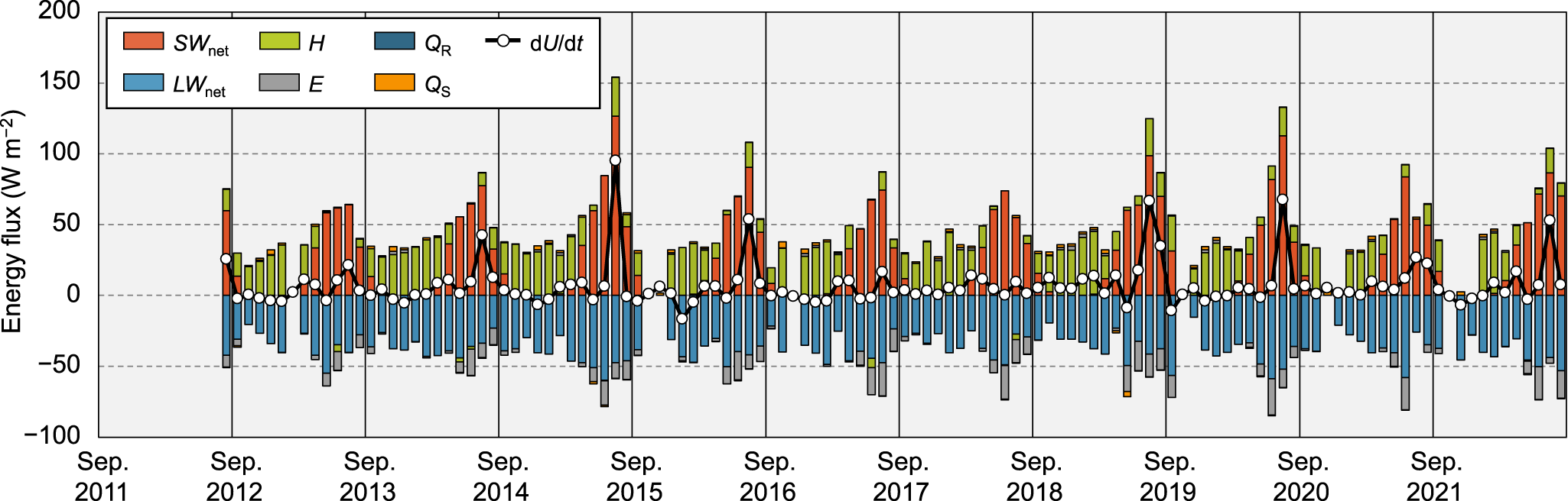
M SEB and R abs in the summers of 2014/15 and 2018/19 exceeded the 1σ range of their standard deviations for all years (Table 3), indicating that the contribution of the radiative components to surface melt was significant. Figure 7 shows the temporal variations in the monthly mean energy flux components. The largest SW net and dU/dt were observed in July 2014/15 (SW net: 126.7 W m−2 and dU/dt: 95.1 W m−2; Table S1). However, in 2018/19, large SW net values comparable to those observed in 2014/15 were not observed during June–August. In contrast, R abs and dU/dt were consistently higher than the monthly averages (R abs; June: 333.7 W m−2, July: 372.2 W m−2 and August: 345.3 W m−2; Table S1). This indicates that SW net was an important component of R abs. In both years LW d was, in absolute terms, the largest contributor and its relative contribution of LW d to R abs was greater in 2018/19 than in 2014/15.
Temporal variation in monthly means of net shortwave radiation (SW net), net longwave radiation (LW net), sensible heat flux (H), latent heat flux (E), rainfall energy flux (Q R), subsurface energy flux (QS) and change in the internal energy of the surface layer (dU/dt).

3.4. Surface mass balance
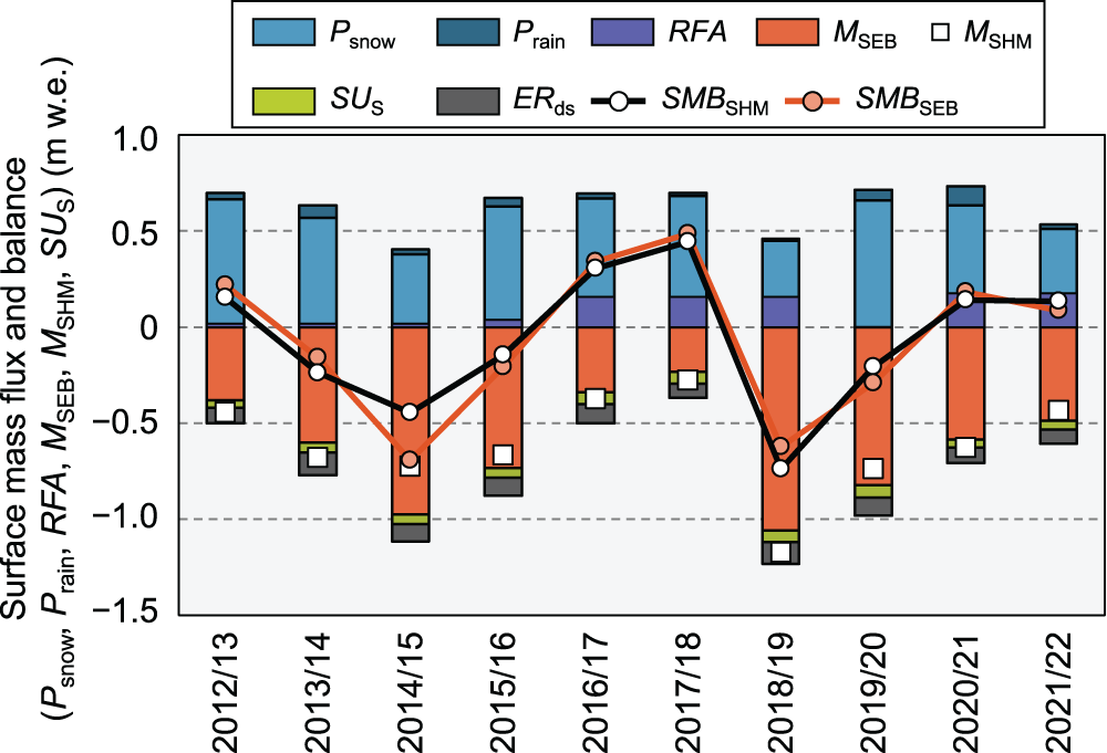
This section presents the SMB variations quantified using two methods: SEB analysis and SHM, the latter being derived from the observed surface height changes. Figure 8 shows the temporal variations in the annual cumulative SMBs and their relevant components. The values presented in Table S2 are summarized in Fig. 8. Significantly lower annual accumulations were observed in 2014/15 (404 mm w.e.) and 2018/19 (452 mm w.e.). The largest ablation amounts (RU + SU s + ER ds) calculated by both methods were observed in 2018/19 (SEB: 1075 mm w.e., SHM: 1191 mm w.e.). In contrast, the lowest annual ablation amounts were calculated in 2017/18 (SEB: 211 mm w.e.; SHM: 256 mm w.e.). The annual mass loss due to ER ds was smaller than that of M SEB, M SHM and the accumulation amount, and showed little variation from year to year (Table S2). The larger negative annual SMBs were calculated for years characterized by a combination of small accumulation and large ablation, which occurred in 2014/15 (SMB SEB: −692 mm w.e.; SMB SHM: −443 mm w.e.) and 2018/19 (SMB SEB: −623 mm w.e.; SMB SHM: −739 mm w.e.).
Temporal variation in annual cumulative amounts of accumulation (P snow and P rain; blue bars), refreezing amount (RFA; purple bars), surface melt amount (M SEB and M SHM; red bar and white box, respectively), water vapor flux (SU s; green bar), snow mass removal by wind erosion (ER ds; gray bar) and surface mass balance (SMB SEB and SMB SHM; orange and white circle plots, respectively). The suffixes ‘SEB’ and ‘SHM’ indicate values calculated using the surface energy balance analysis and surface height method, respectively (see Section 2.2.3).

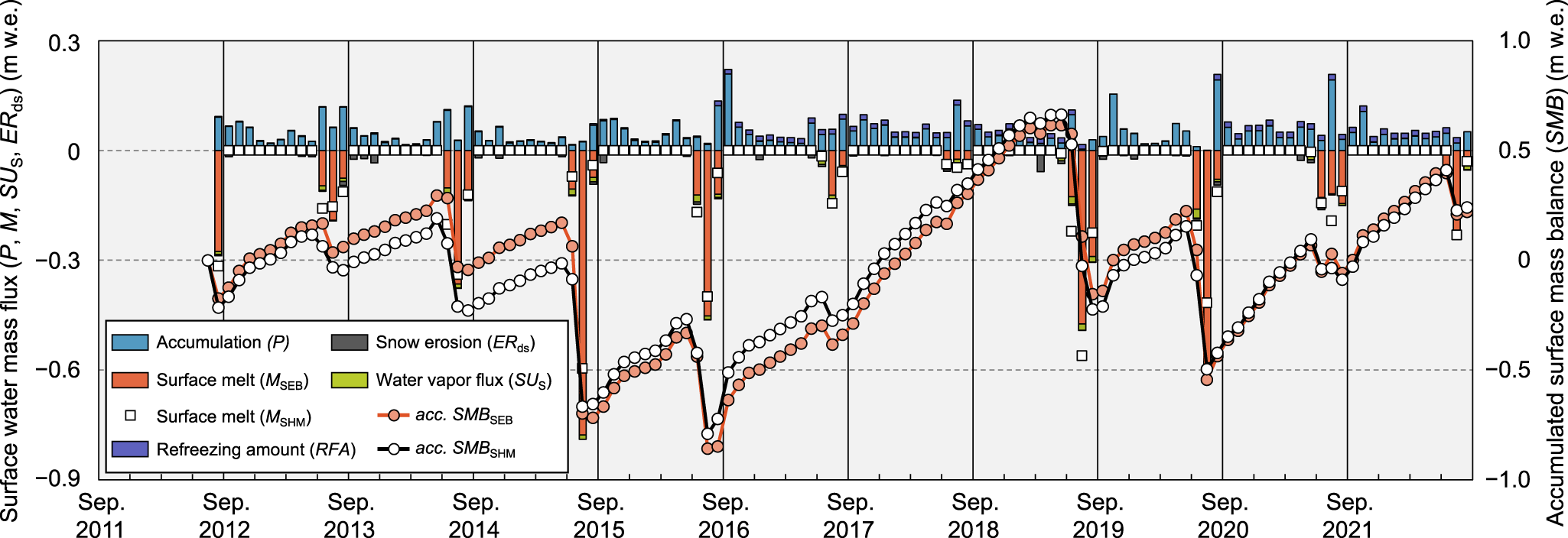
Figure 9 shows the temporal variations in monthly accumulation, ablation amounts and SMB. This result indicates that the cumulative SMB over the entire observation period was slightly positive, with pronounced interannual fluctuations. The cumulative SMBs in August 2022 were +0.26 m w.e. (SEB) and +0.28 m w.e. (SHM), with a difference of 0.02 m w.e.
Temporal variation in monthly cumulative accumulation (P; blue bar), surface melt (M SEB and M SHM; red bar and white box plot), refreezing amount (RFA; purple bars), water vapor flux (SU s; green bar) and snow mass removal by wind erosion (ER ds; gray bar) on the left vertical axis. On the right axis, cumulative surface mass balance variations (SMB SEB and SMB SHM; orange and white circle plots, respectively), with zero at the start of the observation period, are shown.

The interannual SMB variations were largely attributable to the substantial variations in annual ablation amounts (Figs. 8 and 9 and Table S2). The figures show that annual ablation exhibited a greater variability than that exhibited by annual accumulation, with standard deviations of 107.3 (accumulation) and 301.7 and 275.7 (ablation in SEB and SHM, respectively) mm w.e. In particular, a significant decrease in SMB was observed during the summers of 2014/15 and 2018/19, which coincided with periods of large surface melt. These characteristics of the annual SMB variability correspond to the variability of the PDD, the extent of albedo reduction and the amount of radiative energy input, as described in Sections 3.2 and 3.3. In other words, lower accumulation induces albedo reduction, which increases the radiative energy input for surface melting and ablation.
4. Discussion
4.1. Interannual variation surface energy balance
The dataset spanning a decade since 2012 provides results for the SEB analysis, indicating that (1) the peak of surface melt occurs in July and that (2) SW net is the primary energy input driving surface melt, as SW net accounts for approximately 1.8 times the amount of dU/dt in July (Fig. 6). As listed in Table 3, the interannual variation in SW d was small, indicating that the notable decrease in albedo (Fig. 4a) caused an increase in SW net and substantial surface melt during the summers of 2014/15, 2015/16, 2018/19 and 2019/20. Since the decrease in albedo did not occur consistently in July of each year (Fig. 4a), pronounced variability in the monthly mean SW net and dU/dt was observed.
The pronounced decrease in albedo is attributable to the exposure of the underlying ice, which depends on the accumulation of snow in previous years and the magnitude of ablation during summers. The findings indicate that accumulation observed in 2014/15 and 2018/19, both of which exhibited negative annual SMBs, was notably smaller compared to other years (Fig. 8 and Table S2). In addition, a significant snow erosion event occurred in March 2019 (monthly cumulative erosion amount: 57.4 mm w.e.), during which wind erosion removed the snowpack layer. In years with reduced snowfall and snowpack removal caused by wind erosion, the snowpack becomes more susceptible to complete melting during summer, thereby exposing the relatively low-albedo firn layer and ice surface.
At the SIGMA-B site, located near the ELA, surface conditions changed significantly (Fig. 4a). Consequently, the SEB characteristics exhibited substantial annual fluctuations in SW net, dU/dt and total annual melt. Although the meteorological factors controlling the accumulation amount in northwest Greenland remain poorly understood, the factors influencing the ablation amount have been more clearly reported. These include blocking anticyclones (Hanna and others, Reference Hanna, Cropper, Hall and Cappelen2016) and the advection of moist air by atmospheric rivers (Zhu and Newell, Reference Zhu and Newell1998). The influence of these processes on SMB variability is discussed in detail in Section 4.2.
4.2. Drastic surface melt during summers of 2014/15 and 2018/19
A significantly large energy input induced drastic surface mass loss during the summers of 2014/15 and 2018/19 (Table 3 and Fig. 8). These melting events were driven by elevated atmospheric temperatures and radiative processes. In 2014/15, positive albedo feedback associated with snow and ice melting—caused by snow metamorphism and albedo reduction (Aoki and others, Reference Aoki, Kuchiki, Niwano, Kodama, Hosaka and Tanaka2011)—played a major role, whereas cloud radiative forcing (Ramanathan and others, Reference Ramanathan1989) was the dominant contributor in 2018/19.
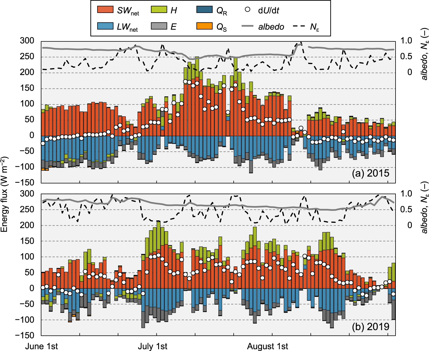
The daily temporal variations in SEB, albedo and N ε during the summers of 2014/15 and 2018/19 (Fig. 10) reveal several notable features. Low albedo and N ε were observed in the summer of 2014/15 (JJA mean: albedo = 0.68, N ε = 0.34; Table 3). In contrast, the summer of 2018/19 did not exhibit a decrease in albedo comparable to that observed in July 2014/15. However, the mean albedo during the summer of 2018/19 was the lowest overall and did not increase until late August, resulting in a high monthly mean SW net in August (Table S1). Moreover, the mean N ε was larger in 2018/19 (JJA: N ε = 0.49) than in 2014/15 (JJA: N ε = 0.34), with the difference being most pronounced in June (0.60).
Temporal variation in daily means of net shortwave radiation (SW net), net longwave radiation (LW net), sensible heat flux (H), latent heat flux (lE), rainfall energy flux (Q R), subsurface energy flux (Q S), change in internal energy of the surface layer (dU/dt), surface albedo and cloud factor (N ε) during the summer seasons of (a) 2015 and (b) 2019.

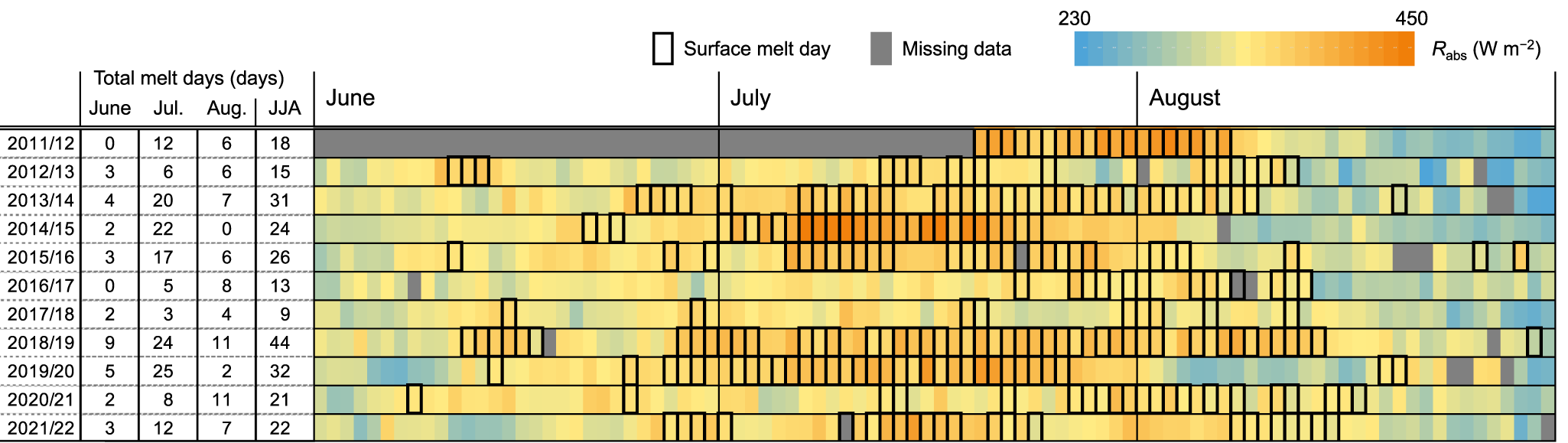
A more detailed analysis of R abs and the number of surface melt days during each summer (Fig. 11) shows that the energy input from R abs led to the greatest amount of surface melt during the summer of 2018/19. As shown in Figs. 10a and 11, during the summer of 2014/15, SW net and R abs exhibited a significant decrease on 5 August because of an increase in albedo due to snowfall, and no surface melt days were observed after 25 July. In contrast, surface melt persisted until 15 August 2018/19. Even earlier in July, R abs values were approximately 350 W m−2 or higher, which were higher than those observed in other years during the same period. Because R abs depends on the amounts of SW net and LW d, decreases in albedo and cloud formation lead to increased R abs through enhanced shortwave and longwave contributions. Thus, the substantial SW net energy input in July 2014/15 was responsible for the second-largest surface melt event, whereas the sustained SW net and LW d (R abs) energy input in the summer of 2018/19 resulted in the highest recorded amount of surface melt during the observation period.
Number of surface melt days with a daily mean surface temperature of 0°C, its distribution and the amount of radiation absorbed by the surface (R abs [W m–2]: a sum of SW net and εLW d) in each summer (June–August). The color map indicates the R abs magnitude, gray areas represent days with missing data and black grid lines represent surface melt days.

As illustrated in Fig. 5, the summers of 2014/15 and 2018/19 exhibited higher PDD values, and albedo values were significantly lower in 2014/15 and 2018/19 than in the other years (Fig. 4a). High air temperatures probably facilitated snow metamorphism and contributed to the reduced albedo. According to the literature, the Greenland Blocking Index (Fang, Reference Fang and Zhu2004) in the summer of 2015 (particularly in July) was high (Hanna and others, Reference Hanna, Cropper, Hall and Cappelen2016), enhancing the high-pressure field over a wide area of Greenland. This high-pressure system transported warm air from the southwest (Hanna and others, Reference Hanna, Cropper, Hall and Cappelen2016) and created atmospheric (clear sky and high air temperature) and surface (low albedo) conditions conducive to extensive melting, particularly in northern Greenland (Tedesco and others, Reference Tedesco2016). As indicated by the N ε values in Table 3 and the LW net frequency distribution reported by Nishimura and others (Reference Nishimura2023), the low cloudiness observed during the 2014/15 summer can be attributed to the blocking anticyclone. Consequently, increased SW net and high air temperatures (Table 3 and Fig. 7) likely triggered positive snow/ice melting feedback, resulting in substantial surface melt during 2014/15, consistent with the findings of Hofer and otheres (Reference Hofer, Tedstone, Fettweis and Bamber2017) and Niwano and others (Reference Niwano, Hashimoto and Aoki2019).
At the SIGMA-B site, snowfall typically occurs around mid-August, which slows down the surface melt process as the albedo increases. However, as illustrated in Fig. 10, the observed 2018/19 summer data indicate that snowfall did not occur until late August, and the albedo remained low. A blocking phenomenon prevailed during the summer of 2018/19 (Hanna and others, Reference Hanna2021), resulting in significant warming across a vast area of Greenland. In particular, the blocking anticyclone that formed over western Europe brought southeasterly winds to northwestern Greenland (Cullather and others, Reference Cullather2020), causing a Foehn event in the northwest. In addition, the albedo decrease in the summer of 2018/19 was exceptional since 2000 (Elmes and others, Reference Elmes2021), due to reduced snowfall associated with blocking anticyclones across Greenland (Tedesco and Fettweis, Reference Tedesco and Fettweis2020). In other words, the low-albedo surface state continued into late August 2019, when downward shortwave radiation gradually decreased (Table 2), while cloud formation during summer (Fig. 10) led to positive cloud radiative forcing, i.e. heating due to enhanced longwave radiation.
A comprehensive analysis of the large melting events that occurred during the summers of 2015 and 2019 was conducted from the perspective of large-scale atmospheric conditions and radiative processes. SEB analysis revealed that warming in both years not only reduced albedo but also increased H. The results showing that the PDD was higher in 2014/15 and 2018/19 than in other years (150 and 177 K days; Fig. 5) support the finding that H was higher in these years than in other years (Table 3). In the summer of 2015, H was largest in July (27.2 W m−2) but was lower than in June and August 2019 (see Table S1 and Fig. 10). In contrast, in the summer of 2019, H in July and August was higher than in other years (July: 26.2 W m−2, August: 16.7 W m−2). The warming and increase in H during the summers of 2015 and 2019 coincided with an anticyclone-blocking field. In addition, the Foehn phenomenon was caused by southeasterly winds during the summer of 2019. Although the energy contribution of H was lower than that of the radiative compounds, this study demonstrated that H is a major positive energy source and shows considerable interannual variability. This finding indicates that variations in large-scale climate conditions that induce substantial melting not only affect the absorbed radiative fluxes but also H, thereby emphasizing the significance of H in the context of snow and ice melt.
The atmospheric blocking that drove the rise in air temperature and extensive melt in 2014/15 and 2018/19 is known to have a negative correlation with the North Atlantic Oscillation (NAO; Hanna and others, Reference Hanna, Cropper, Jones, Scaife and Allan2015). The NAO has also been reported to have strong relationships with the Atlantic Multidecadal Oscillation (AMO) and the Atlantic Meridional Overturning Circulation (Hanna and others, Reference Hanna2013; Delworth and others, Reference Delworth, Zeng, Zhang, Zhang, Vecchia and Yang2017). Positive feedback between increasing sea surface temperatures and reductions in sea ice associated with the AMO can amplify Arctic air temperatures through a process known as Arctic Amplification. This warming can enhance the atmospheric supply of water vapor (Nusbaumer and others, Reference Nusbaumer, Alexander, LeGrande and Tedesco2019) and induce cloud formation (Palm and others, Reference Palm, Strey, Spinhirne and Markus2010), as suggested by Screen and Simmonds (Reference Screen and Simmonds2010). Increased atmospheric water vapor and cloud cover have been widely reported to cause surface heating of the Greenland ice sheet through radiative forcing (Niwano and others, Reference Niwano, Hashimoto and Aoki2019; Silva and others, Reference Silva, Abermann, Noël, Shahi, van de Berg and Schöner2022), reaffirming the importance of comprehensively understanding the interactions between the atmosphere, ocean and land (glaciers) in the North Atlantic, including Greenland.
4.3. Surface mass balance around ELA on Qaanaaq Ice Cap
During the observation period, a positive annual mass balance was recorded for many years. However, the annual mass balances were negative in 2014/15 and 2018/19, corresponding to years of significant ablation (Fig. 8). Consequently, the cumulative SMB over the entire observation period was only slightly positive, with estimated values of +0.26 m w.e. (SEB) and +0.28 m w.e. (SHM). Field observations and surface height data further corroborated that the ice layer under the snowpack formed closer to the surface. This finding, consistent with previous studies by Tsutaki and others (Reference Tsutaki, Sugiyama, Sakakibara, Aoki and Niwano2017) and Sugiyama and others (Reference Sugiyama2021), which placed the ELA between 700 and 1000 m a.s.l., supports the present results indicating a small positive mass balance at the SIGMA-B site (944 m a.s.l.).
The results of this study indicate that the ELA of the Qaanaaq Ice Cap, where the SIGMA-B site is located, is slightly lower than 944 m from the period between 2012 and 2022. However, because the elevation of the ELA defined by the mass balance varies depending on the geographical location and climatic conditions, it must be interpreted in conjunction with the environmental context of the target region. As reference, previous ELA quantifications summarized as follows. In the Canadian Arctic’s Queen Elizabeth Islands (latitude: 75–80°N), glaciers and ice caps above 1000 m reported an average ELA of 840 (±70) m over the 60-year period from 1960s to 2010s (Burgess and Danielson, Reference Burgess and Danielson2022). However, in the Svalbard islands (78–79°N), where elevations are lower, reports indicate ELAs of 400–700 m (Schmidt and others, Reference Schmidt, Schuler, Thomas and Westermann2023). Additionally, Securo and others (Reference Securo2024) reported that the ELAs of ice caps larger than 1 km2 in central and southwestern Greenland from 2018 to 2022 were 1260–1510 m in the central region (69–73°N) and 1050–1125 m in the southern region (63–67°N). Previous research in northwestern Greenland showed that the ELA at the Freya Glacier (74°N) between 2008 and 2013 was approximately 1000 m (Hynek and others, Reference Hynek, Weyss, Binder, Schöner, Abermann and Citterio2014; Machguth and others, Reference Machguth2016). In addition, for the A.P. Olsen Ice Cap in northeastern Greenland (74°N; Citterio and others, Reference Citterio, Andersen, Larsen, Kristensen, Skourup, Ahlstrøm, Jensen, Rasch and Schmidt2013), the end-of-summer snow line altitude (SLA; synonymous with ELA here) was 1150 m between 2008 and 2024 (Rutishauser and others, Reference Rutishauser, Larsen, Karlsson, Binder, Hynek and Citterio2025). When these regions were compared with the Qaanaaq Ice Cap (78°N, assuming an ELA of approximately 900 m), SMB analysis from Svalbard (Schmidt and others, Reference Schmidt, Schuler, Thomas and Westermann2023) indicated a lower ELA than that of the Qaanaaq Ice Cap, possibly due to the lower summer melt rates. Conversely, ELAs in southwestern and northeastern Greenland, which are at lower latitudes, were higher than those of the Qaanaaq Ice Cap. The ice caps in the Canadian Arctic, which are similar in latitude and elevation, have ELAs that are relatively similar to those of the Qaanaaq Ice Cap. These findings support the validity of the ELA assessment at the SIGMA-B site. At the A.P. Olsen Ice Cap, annual accumulation has been below 500 mm w.e. for many years (Rutishauser and others, Reference Rutishauser, Larsen, Karlsson, Binder, Hynek and Citterio2025), lower than that at the SIGMA-B site (Table S2). In addition, no significant temperature difference was observed between the SIGMA-B and AWS sites (AWS2) on the A.P. Olsen Ice Cap (Nishimura and others, Reference Nishimura2023; Larsen and others, Reference Larsen, Binder, Rutishauser, Hynek, Fausto and Citterio2024). Therefore, differences in ELA between eastern and western northern Greenland may primarily reflect variations in annual accumulation.
ELA is a variable that changes over the long term and is currently rising with increasing temperatures (e.g. Ohmura and Boettcher, Reference Ohmura and Boettcher2022). Securo and others (Reference Securo2024) analyzed data from the 1980s and 2018–2022 and found that the ELA increase was faster in central-western Greenland than that in south-western Greenland. The 10-year analysis in this study did not reveal any long-term SMB variations and therefore could not provide insights into long-term ELA trends. Nevertheless, summer temperatures clearly play a significant role in determining glacier ELA (e.g. Ahlmann, Reference Ahlmann1924; Ohmura and Boettcher, Reference Ohmura and Boettcher2018). Consequently, the SIGMA-B site, located near the ELA, is crucial for investigating SMB changes and ELA variations on the Qaanaaq Ice Cap and northwestern Greenland glaciers under future climate change scenarios.
Increasing air temperatures in the cryosphere, as typified by Arctic Amplification, have caused various environmental changes, including decreases in albedo and shifts in precipitation phase. If this trend continues, mass loss may accelerate in the mid-elevation zones of coastal ice caps, such as near the SIGMA-B site. Although increased precipitation can enhance future accumulation (McCrystall and others, Reference McCrystall, Stroeve, Serreze, Forbes and Screen2021), it is likely that precipitation will fall as rain in the peripheral ice cap areas of Greenland, where temperatures are higher than those observed on the inland ice sheet. A polar regional climate model (NHM-SMAP) simulations demonstrated an increase in rainfall in northwestern Greenland from 1980 to 2019 (Niwano and others, Reference Niwano, Box, Wehrlé, Vandecrux, Colgan and Cappelen2021). In addition, model simulations indicate that firn layer reduction leads to significant mass loss in the peripheral regions of the ice sheet, where declining water retention capacity limits storage of meltwater and rainwater (Noël and others, Reference Noël2017, Reference Noël, Lenaerts, Lipscomb, Thayer-calder and van den Broeke2022). Previous studies have shown that rising temperatures reduce snowfall, accelerate firn melting and expand ablation zones (Noël and others, Reference Noël, van de Berg, Lhermitte and van den Broeke2019), exposing the ice surface beneath the firn layer. The results of this study suggest that if ‘Arctic Amplification’ continues, mass loss will further accelerate.
5. Conclusion
The objective of this study was to clarify the actual state of mass loss around the ELA of peripheral glaciers in northwest Greenland, where rapid warming occurs. To this end, in situ AWS (SIGMA-B site; 944 m a.s.l.) observational data from the Qaanaaq Ice Cap were used to determine the interannual variations in the surface energy and mass balance (SEB and SMB) over a decade from July 2012 to September 2022. The amount of surface melting was calculated using full SEB analysis and the SHM. The SMB was determined by calculating the snow accumulation and subsequent surface height changes, taking into account wind erosion and snow drift, snow densification and surface sublimation. The results indicated that (1) the snow layer melted during the 2014/15 and 2018/19 summers, exposing the ice surface and resulting in a significant decrease in surface albedo and surface mass loss; (2) melting in 2015 was triggered by enhanced shortwave radiation resulting from a decrease in albedo caused by higher air temperatures (a typical snow/ice positive albedo feedback), whereas the melting in 2019 was driven by not only shortwave radiation but also downward longwave radiation heating (the cloud radiative forcing effect); (3) the annual surface SMBs varied considerably; however, the net SMB was slightly positive (SEB: +0.26 and SHM: +0.28 [m w.e.]) over the decade.
At mid-altitude sites (such as the SIGMA-B site) in peripheral Greenland, future temperature increases could change the precipitation phase from snow to rain, leading to a decrease in snowfall. Consequently, the exposure of ice surfaces is likely to occur more frequently in the future, as observed in 2015 and 2019, and significant surface mass losses can be expected. Field observations should continue to provide deeper insights into environmental changes.
Supplementary material
The supplementary material for this article can be found at https://doi.org/10.1017/jog.2026.10159.
Acknowledgements
A considerable number of individuals provided invaluable assistance during the study in Greenland. We express our gratitude to everyone involved in this study. In particular, Tetsuhide Yamasaki made notable contributions over a long period in the areas of field logistics, safety management and AWS installation in Greenland, and Tomoki Kajikawa contributed to AWS maintenance. We would like to express our gratitude to these individuals. Dr Shun Tsutaki provided the SMB data from stake observations of the Qaanaaq Glacier to evaluate the SMB analysis. We would also like to express our gratitude to Navarana K’avigak for providing us with a residence as a base for our observations and to Sakiko Daorana for her invaluable assistance in Qaanaaq Village. We would also like to express our gratitude to Dr Carleen Reijmer, the scientific editor of this paper, and two anonymous reviewers for their insightful comments, which contributed to enhancing the quality of this manuscript. This study was conducted as part of the ‘Snow Impurity and Glacial Microbe effects on abrupt warming in the Arctic (SIGMA)’ Project supported by the Japan Society for the Promotion of Science (JSPS), Grant-in-Aid for Scientific Research (Grant numbers: JP24K20922, JP23221004, JP16H01772, JP17KK0017 and JP21H03582), the Arctic Challenge for Sustainability II (ArCS II; Grant number: JPMXD1420318865), the Arctic Challenge for Sustainability 3 (ArCS-3; Grant number: JPMXD1720251001), the Ministry of the Environment of Japan through the Experimental Research Funds for Global Environment Conservation MLIT2253 and the Global Change Observation Mission-Climate (GCOM-C) research project of JAXA. In addition, a map (Fig. 1) was created using the National Snow and Ice Data Center QGreenland package (Moon and others, Reference Moon, Fisher, Harden and Stafford2021). The DEM data were attributed to Arctic DEMs provided by the Polar Geospatial Center under NSF-OPP awards 1043681, 1559691 and 1542736.


 Open access