2. Models and theoretical setup

In this work, we focus on granular lattice dynamical systems. The non-dimensional equations of motion (where the constant elastic and geometric prefactors have been absorbed through a suitable rescaling) is given by the following differential-difference equations (DDEs) Nesterenko [Reference Nesterenko39].

(2.1)\begin{equation} \ddot u_{n} = \left[\delta_{0} + u_{n-1} -u_{n}\right]^{p}_{+} - \left[\delta_{0} +u_{n}-u_{n+1}\right]^{p}_{+}, \end{equation}

where δ ₀ denotes the precompression constant, u_n is the displacement of the nth particle from its equilibrium position, and $\left[f\right]_{+} = \text{max}(f,0)$, models the fact that there is no force when the particles come out of contact. The case of $p=3/2$ corresponds to a lattice of spherical particles. It is relevant to mention in passing that in other settings such as O-rings, cylindrical particles or hollow spheres the nature of the force (and hence exponent) may vary Johnson [Reference Johnson30] and hence we will maintain p as a general parameter in our considerations herein. Equation (2.1) possesses travelling wave solutions Nesterenko [Reference Nesterenko39]; Sen et al. [Reference Sen, Hong, Bang, Avalos and Doney42]; Starosvetsky et al. [Reference Starosvetsky, Jayaprakash, Arif Hasan and Vakakis45]; Chong and Kevrekidis [Reference Chong and Kevrekidis9], even though their exact form is not known analytically (but for relevant approximations see e.g., Starosvetsky and Vakakis [Reference Starosvetsky and Alexander44]). Moreover, numerical investigations of Eq. (2.1) reveal the formation of dispersive shocks in certain regimes Herbold and Nesterenko [Reference Herbold and Nesterenko23a]; [Reference Herbold and Nesterenko24b]; Molinari and Daraio [Reference Molinari and Daraio38]; Yasuda et al. [Reference Yasuda, Chong, Yang and Kevrekidis53]. In a recent work, we studied the DSWs produced by Eq. (2.1) when $\delta_0\ne0$, making use of two different (integrable) approximations for it: the Toda lattice and the Korteweg-de Vries equation Chong et al. [Reference Chong, Geisler, Kevrekidis and Biondini7]. In the present work, we focus on the case where $\delta_{0}=0$, in which case the model does not admit a meaningful linear limit in the case of zero background.

It will be convenient to work with the strain variable $r_{n} = u_{n-1} - u_{n}$, which has a physically meaningful interpretation in terms of granular crystals (the amount of compression between adjacent particles), and is common when describing granular crystals, see, e.g., the authoritative book of Nesterenko [Reference Nesterenko39]. We note in passing, however, that some authors also use the variable $u_{n} - u_{n-1}$ for the relevant analysis Dreyer et al. [Reference Dreyer, Herrmann and Mielke13]. In terms of the strain, Eq. (2.1) becomes

(2.2)\begin{equation} \ddot r_{n} = \left(r_{n+1}\right)^{p} - 2\left(r_{n}\right)^{p} + \left(r_{n-1}\right)^{p}, \end{equation}

where we dropped (here and henceforth) the subscript + under the assumption that the strains are non-negative. The linearized dispersion relation for small-amplitude wave solutions of the form $r_n(t) = A + B e^{i(kn - \omega t)}$, with $|B/A| \ll 1$, is given by:

(2.3)\begin{equation} \omega^2 = 4pA^{p-1} \sin^2\left(\frac{k}{2}\right), \end{equation}

where k and ω are the wavenumber and frequency, respectively.

Conversely, DSWs, which are one the main concerns of this paper, arise in Eq. (2.2) when initialized with Riemann initial data

(2.4)\begin{equation} r_n(0) = \begin{cases} r_-, \quad & n \leq 0 \\ r_+, \quad & n \gt 0 , \end{cases} \qquad \dot{r}_n(0) = \begin{cases} v_-, \quad & n \leq 0 \\ v_+, \quad & n \gt 0 . \end{cases} \qquad \end{equation}

We wish to use a dispersive long-wavelength model to approximate (2.2). To this end, we introduce an associated smallness parameter $0 \lt \epsilon \ll 1$ and the following slowly varying spatial and temporal variables

(2.5)\begin{equation} X = \epsilon n, \qquad T = \epsilon t. \end{equation}

Using the ansatz $r_{n}(t) = r(X,T)$ and substituting into Eq. (2.2) leads to:

(2.6)\begin{equation} \epsilon^{2}r_{TT} = r^{p}(X+\epsilon,T) + r^{p}(X-\epsilon,T) - 2r^{p}(X,T). \end{equation}

A Taylor expansion of Eq. (2.6) then yields, to leading order, the partial differential equation (PDE):

(2.7)\begin{equation} r_{TT} = \left(r^{p}\right)_{XX}. \end{equation}

Equation (2.7) was already studied in Yasuda et al. [Reference Yasuda, Chong, Yang and Kevrekidis53] (see also its earlier derivation in Chong et al. [Reference Chong, Kevrekidis and Schneider10]), where it was shown to correctly capture the wave breaking in the solutions of Eq. (2.2). However, Eq. (2.7) is a non-dispersive model, and as such it does not give rise to the formation of DSWs. Indeed, looking for small-amplitude plane-wave solutions of Eq. (2.7) in the form $r(X,T) = A + B \,e^{i(K X - \Omega T)}$, where $|B/A|\ll1$ and K and Ω are the wavenumber and frequency with respect to the variables $X,T$, yields the linearized dispersion relation $\Omega^2 = pA^{p-1}\,K^2$, for which $d^2\Omega/dK^2\equiv0$ (hence the PDE is non-dispersive). Note that we can relate the wavenumber and frequency of the PDE model to those of the original lattice variables through the relationship

(2.8)\begin{equation} K= \epsilon^{-1} k, \qquad \Omega= \epsilon^{-1} \omega. \end{equation}

In order to be able to describe DSWs, we include next order in the Taylor expansion of Eq. (2.6) by keeping terms up to $\mathcal{O}\left(\epsilon^{2}\right)$. Doing so yields the PDE

(2.9)\begin{equation} r_{TT} = \left(r^{p}\right)_{XX} + \frac{\epsilon^{2}}{12}\left(r^{p}\right)_{XXXX}. \end{equation}

This model, originally proposed in Ahnert and Pikovsky [Reference Ahnert and Pikovsky2], is ill-posed, however, due to large wavenumber instabilities. Indeed, looking for plane-wave solutions as before yields $\Omega^2 = p A^{p-1} K^2 ( 1 - \frac1{12} \epsilon^2 K^2)$. Note that Ω is purely imaginary for sufficiently large wavenumbers (i.e., $|K| \gt 2\sqrt{3}/\epsilon$). Thus, small wavelength oscillations are unstable. Moreover, the imaginary part of Ω is unbounded. Therefore, it is expected that Eq. (2.9) is ill-posed as an initial-value problem.

On the other hand, Eq. (2.9) can be regularized in a straightforward way, following Rosenau [Reference Rosenau40]; [Reference Rosenau41]. In particular, since

(2.10)\begin{equation} r_{TT} = \left(r^{p}\right)_{XX} + \frac{\epsilon^{2}}{12}\left(r^{p}\right)_{XXXX} = \left(r^{p}\right)_{XX} + \mathcal{O}(\epsilon^{2}), \end{equation}

we have that

(2.11)\begin{equation} \left(r^{p}\right)_{XXXX} = \left(\left(r^{p}\right)_{XX}\right)_{XX} = \left(r_{TT} - \mathcal{O}(\epsilon^{2})\right)_{XX} = r_{TTXX} + \mathcal{O}(\epsilon^{2}). \end{equation}

The substitution of (2.11) into (2.10) then yields, up to $\mathcal{O}\left(\epsilon^{4}\right)$ terms

(2.12)\begin{equation} r_{TT} - \frac{\epsilon^{2}}{12}r_{XXTT} = \left(r^{p}\right)_{XX}. \end{equation}

If we now look for plane wave solutions of (2.12), we obtain:

(2.13)\begin{equation} \Omega^2 = \frac{pA^{p-1}K^2}{\left(1 + \frac{\epsilon^2}{12}K^2\right)}, \end{equation}

which is a perfectly well-behaved dispersion relation, real-valued for all $K\in\mathbb{R}$. Figure 1 shows Eq. (2.13) compared to Eq. (2.3) and other relevant approximations (see below). Note that the PDE dispersion relations are independent of ϵ if expressed in terms of the original lattice variables (using Eq. (2.8)).

Figure 1.

Comparison of the linearized dispersion relations of different models in terms of $(k,\omega)$. The solid blue line corresponds to the lattice dispersion relation (2.2), with Brillouin zone given by $[0,\pi]$. We show larger wavenumbers for comparison purposes. The red dotted curve is the dispersion relation of (2.9) (and (3.11), which happens to be identical). For $k \gt 2 \sqrt{3}$ we see that $\omega^2 \lt 0$, which leads to ultraviolet (i.e., high wavenumber) instability and ultimately ill-posedness. The black dashed curve depicts the linearized dispersion relation of the regularized model (2.12), which has a horizontal asymptote ( $\omega^2 \rightarrow 24$ for the specific values used here). For all curves, the parameters are chosen to be $p = 2, A = 1$.

An additional interesting observation here is that even when the model is nonlinearly dispersive with p ≠ 1, the additional dispersive effects of $\mathcal{O}\left(\epsilon^{2}\right)$ appear at the linear level herein. This is distinct from the previously proposed continuum approximations such as those of Ahnert and Pikovsky [Reference Ahnert and Pikovsky2], as well as that of Nesterenko [Reference Nesterenko39], where the continuum limit is taken at the level of displacements, rather than that of strains. We will compare these different models further, e.g., at the level of their travelling waves in the next section.

Equation (2.12) is the primary model of interest in this work. In particular, we will show that Eq. (2.12) accurately captures, both qualitatively and quantitatively, the solitary waves, periodic travelling waves and DSWs of Eq. (2.1). Recall that Zabusky and Kruskal derived the Korteweg-de-Vries (KdV) equation with small dispersion as a long-wave approximation of the Fermi-Pasta-Ulam-Tsingou (FPUT) problem Zabusky and Kruskal [Reference Zabusky and Kruskal54]; Gallavotti [Reference Gallavotti20]. We claim that (2.12) plays for the granular lattice model (2.2) a similar role that the KdV equation plays for the FPUT problem. Specifically, the claim is that, just like the KdV equation provided a useful continuum model to describe, at least in the long-wave limit, the dynamics of solutions of the FPUT problem, so does the PDE (2.12) for the granular lattice model (2.2).

3. Solitary wave solutions

While the ultimate goal of this work is to characterize the DSWs of the granular chain, to do so we must first review its solitary waves and periodic travelling wave solutions. We delve into the analysis of these states in this and the next section.

3.1. Derivation of solitary waves

Our first goal is to find the travelling solitary wave corresponding to the model (2.12). To this end, we first introduce the travelling wave ansatz, namely

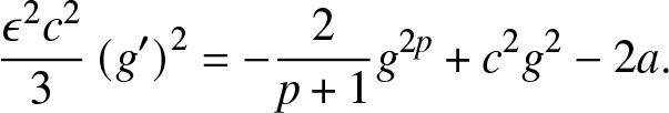
(3.1)\begin{equation} r(X,T) = {R\left(Z\right),\qquad Z = X - cT.} \end{equation}

Substituting this ansatz in (2.12), integrating twice (using a suitable integrating factor) yields

(3.2)\begin{equation} \frac{\epsilon^{2}c^{2}}{12}\left(R'\right)^{2} = -\frac{2}{p+1}R^{p+1} + c^{2}R^{2} - 2aR - b, \end{equation}

where $'$ denotes differentiation with respect to Z throughout this section, and $a, b$ are two integration constants. When p takes on half-integer values, it is convenient to apply the transformation $R = g^{2}$ so that Eq. (3.2) becomes

(3.3)\begin{equation} \frac{\epsilon^{2}c^{2}}{3}g^{2}\left(g'\right)^{2} = -\frac{2}{p+1}g^{2\left(p+1\right)} + c^{2}g^{4} - 2ag^{2} -b. \end{equation}

To compute the associated travelling wave solution, we need b = 0, given its decay at infinity. Then, we can divide both sides of Eq. (3.3) by g ² to obtain

(3.4)\begin{equation} \frac{\epsilon^{2}c^{2}}{3}\left(g'\right)^{2} = -\frac{2}{p+1}g^{2p} + c^{2}g^{2} - 2a. \end{equation}

To compute the associated travelling wave solution to Eq. (3.4), the decay of the solution again requires a = 0 so the solution, obtained via quadrature, reads

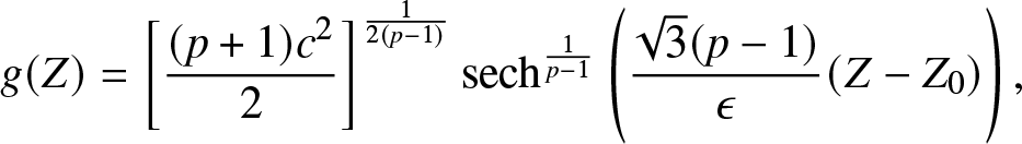(3.5)\begin{equation} g(Z) = \left[\frac{(p+1)c^{2}}{2}\right]^{\frac{1}{2(p-1)}}\text{sech}^{\frac{1}{p-1}}\left(\frac{\sqrt{3}(p-1)}{\epsilon}(Z-Z_{0})\right), \end{equation}

where Z ₀ is an integration constant. Indeed, the relevant calculation arises in the process of identifying the bright solitary waves of the general power variant of the nonlinear Schrödinger equation Sulem and Sulem [Reference Sulem and Sulem47]. Recall that since $R = g^{2}$, the corresponding travelling wave solution for R assumes the form

(3.6)\begin{equation} R(Z) = \left[\frac{(p+1)c^{2}}{2}\right]^{\frac{1}{p-1}}\text{sech}^{\frac{2}{p-1}}\left(\frac{\sqrt{3}(p-1)}{\epsilon}(Z-Z_{0})\right). \end{equation}

Written in terms of the original granular (strain) variable, this becomes,

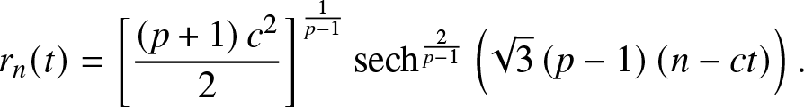(3.7)\begin{equation} r_n(t) = \left[\frac{\left(p+1\right)c^{2}}{2}\right]^{\frac{1}{p-1}}\text{sech}^{\frac{2}{p-1}}\left(\sqrt{3}\left(p-1\right)\left(n - ct\right)\right). \end{equation}

Note that the solitary wave approximation is independent of the parameter ϵ.

3.2. Comparison of travelling waves of different models

We now perform a comparison of the travelling wave solutions corresponding to different approximate models for the granular chain, including Eq. (2.12), the model of Eq. (2.9) proposed in the work of Ahnert and Pikovsky [Reference Ahnert and Pikovsky2] and finally the earliest continuum approximation from the classic work of Nesterenko [Reference Nesterenko39] (through the continuum limit in displacements). The work of Ahnert and Pikovsky [Reference Ahnert and Pikovsky2] already compared the latter two continuum models with the numerically exact travelling lattice solution. For completeness, we also remind the reader the form of the travelling wave solution for these other 3 models (2 continuum approximations, namely Ahnert and Pikovsky [Reference Ahnert and Pikovsky2] and Nesterenko [Reference Nesterenko39], as well as for the original lattice model) in what follows.

Using the travelling wave ansatz (3.1) in Eq. (2.9) of Ahnert and Pikovsky [Reference Ahnert and Pikovsky2], we reduce it to the following ODE,

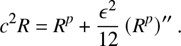(3.8)\begin{equation} c^{2}R = R^{p} + \frac{\epsilon^{2}}{12}\left(R^{p}\right)''. \end{equation}

The solution to Eq. (3.8) reads

(3.9)\begin{equation} R(Z) = |c|^{m}A_{1}\cos^{m}\left(B_{1}Z\right), \end{equation}

where

(3.10)\begin{equation} m = \frac{2}{p-1},\qquad A_{1} = \left(\frac{p+1}{2p}\right)^{\frac{1}{1-p}}, \qquad B_{1} = \frac{\sqrt{3}}{\epsilon}\frac{p-1}{p}. \end{equation}

Importantly, note that Eq. (3.9) applies only between two consecutive zeros of the cosine, beyond which R(z) is taken to be identically zero. The same is true for Eq. (3.13) below. Similarly, the classical continuum PDE model of Nesterenko [Reference Nesterenko39] reads

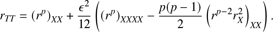(3.11)\begin{equation} r_{TT} = \left(r^{p}\right)_{XX} + \frac{\epsilon^{2}}{12}\left(\left(r^{p}\right)_{XXXX} - \frac{p(p-1)}{2}\left(r^{p-2}r^{2}_{X}\right)_{XX}\right). \end{equation}

Substituting the travelling wave ansatz (3.1) into Eq. (3.11) yields

(3.12)\begin{equation} c^{2}R = R^{p} + \frac{\epsilon^{2}}{12}\left(R^{p}\right)'' - \frac{\epsilon^{2}p(p-1)}{24}R^{p-2}\left(R'\right)^{2}. \end{equation}

The solution to Eq. (3.12) reads

(3.13)\begin{equation} R(Z) = |c|^{m}A_{2}\cos^{m}\left(B_{2}Z\right), \end{equation}

where

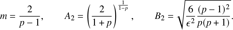(3.14)\begin{equation} m = \frac{2}{p-1}, \qquad A_{2} = \left(\frac{2}{1+p}\right)^{\frac{1}{1-p}}, \qquad B_{2} = \sqrt{\frac{6}{\epsilon^{2}}\frac{(p-1)^{2}}{p(p+1)}}. \end{equation}

As discussed above, we also wish to compare the results of the proposed model (2.12) with the numerically computed exact travelling wave solution of the original granular chain. These are solutions of the form $r_n(t) = r(n- ct) = r(z)$ where r(z) satisfies the advance-delay equation

(3.15)\begin{equation} c^2 r'' = r^p(z-1) - 2 r^p(z) + r^p(z+1). \end{equation}

To this end, we applied an iterative algorithm Hochstrasser et al. [Reference Hochstrasser, Mertens and Büttner25] to numerically compute the solutions of Eq. (3.15), see also Chong and Kevrekidis [Reference Chong and Kevrekidis9]. Note that when we refer to the “exact” solution, we are referring to the numerical solution found to a specified numerical tolerance of Eq. (3.15).

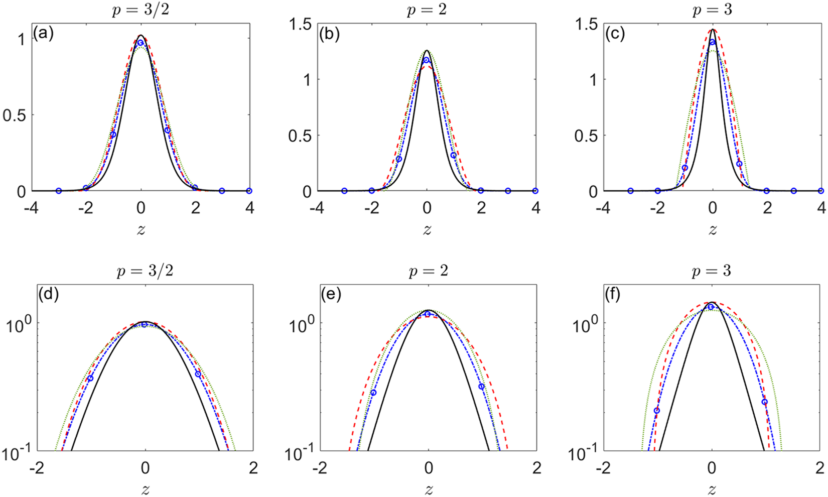
Figure 2 showcases the numerical comparison of four travelling wave solutions (3 approximations and 1 “exact” – again, to a prescribed tolerance) for the cases of $p = 3/2$, 2, 3. Each of the travelling wave solutions which arise in periodic (cosinusoidal) form is plotted only for one period of the corresponding cosine function, beyond which the solution is taken to be zero. Note that, while the continuum models themselves depend on the parameter ϵ, the corresponding prediction is independent of ϵ once one returns to the original lattice variables, see e.g. Eq. (3.7). Thus, we do not need to “select” any particular value of ϵ when comparing solitary waves.

For the values of p considered here, the approximation from (3.7) is meaningfully proximal to the exact solution, as are the other models. See the black solid curve of Fig. 2. In terms of the error $E=\frac{1}{N}\sum_n^N |r_n - R(\epsilon n)|$, where r_n is an “exact” travelling wave and R a travelling wave from one of the PDE models, the approximation errors are of the same magnitude. For example, with $p=3/2$ the errors are E = 0.034 for the strain variant of the model of Nesterenko (3.11), E = 0.030 for the model of Ahnert-Pikovsky (2.9), and E = 0.046 for the model considered in this paper, namely the regularized model of (2.12). The errors for other values of p are similar. We notice that although the error of the model (2.12) is the greatest, it is still quite small and also comparable to the other two. Recall that the solitary wave solution of the granular chain has a double exponential decay in the tails Chatterjee [Reference Chatterjee6]; English and Pego [Reference English and Pego18], whereas the approximation from (3.7) has only exponential decay. The approximations (3.9) and (3.13) have finite support. See Fig. 2(d–f), which shows the solutions in a semi-log scale where the decay rate can be better discerned. While the quantitative differences between the actual solution and approximation are similar for all cases, it still remains an interesting open question if, in terms of rigorous error bounds, any of the three considered here is the “most” accurate. It is worth mentioning that here we have only examined the stationary (in the co-travelling frame) aspect of solitary waves. Towards the end of our presentation, we will return to the dynamical properties of these models, as concerns the prototypical structure considered herein, namely the DSW.

Figure 2.

Comparison of the travelling solitary waves in different continuum models for different values of the parameter p: The leftmost, middle, and rightmost columns denote the cases of $p = 3/2, 2, 3$, respectively. The blue lines (with circles) denote the “exact” solitary wave of Eq. (3.15), and the red dashed line, green dotted line, black solid line refer to the solitary waves associated with the Ahnert-Pikovsky (2.9), Nesterenko (3.11), and the regularized continuum model (2.12), respectively. The first row shows the comparison of the solitary waves of different continuum models in their respective standard scale, while the second row depicts the semi-log scale of all solitary waves. Note that Ahnert-Pikovsky’s and Nesterenko’s approximations for the solitary waves are only plotted over the period of the respective cosine.

4. Periodic travelling wave solutions

Next, we look for periodic solutions, which as usual will play a crucial role in the study of DSWs. In particular, we seek solutions to Eq. (3.4) with a ≠ 0. Unlike the solitary wave solutions, however, where we were able to obtain solutions for arbitrary values of p, in this case the calculations (and the resulting expressions) are dependent on the specific value of p. Here we will focus on three special cases: $p = 3/2$, p = 2 and p = 3. In the following three subsections, we only list the analytical expression of the periodic wave solutions for each of the three cases and defer the detailed derivation of these solutions to Appendix A.

4.1. Case $p = 3/2$

When $p = 3/2$, the original ODE (3.4) becomes

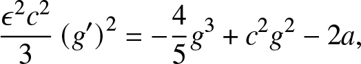(4.1)\begin{equation} \frac{\epsilon^{2}c^{2}}{3}\left(g'\right)^{2} = -\frac{4}{5}g^{3} + c^{2}g^{2} - 2a, \end{equation}

where, as before, primes denote differentiation with respect to Z. A direct integration of Eq. (4.1) yields,

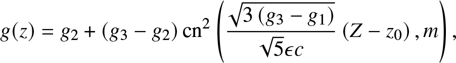(4.2)\begin{equation} g(z) = g_2 + \left(g_3 -g_2\right)\text{cn}^{2}\left( \frac{\sqrt{3\left(g_3 - g_1\right)}}{\sqrt{5}\epsilon c}\left(Z-z_0\right), m\right), \end{equation}

where $\text{cn}\left(Z,m\right)$ denotes the Jacobi elliptic cosine function with parameter m ( $\sqrt{m}$ is the modulus), and $g_1, g_2, g_3$ the three roots of the potential curve $P\left(g\right) = -g^{3} + \frac{5}{4}c^{2}g^{2} - \frac{5}{2}a$, and $m = \frac{g_3 - g_2}{g_3 - g_1}$.

Finally, since $R = g^{2}$, we solve for R to get the following periodic solution,

(4.3)\begin{equation} R(Z) = \left[g_{2} + \left(g_{3} - g_{2}\right)\text{cn}^{2}\left( \frac{\sqrt{3\left(g_3 - g_1\right)}}{\sqrt{5}\epsilon c}\left(Z-z_0\right), m\right)\right]^{2}. \end{equation}

Note that this is only a two-parameter family of periodic waves, and hence is not the most general form. In the derivation of this formula, one of the integration constants was set to zero, see Eq. (4.1). We were unable to find an analytical formula for the general, three parameter, case.

4.2. Case p = 2

When p = 2 we do not need to apply the transformation $R = g^2$, so we simply focus on the original ODE (3.2) which now becomes:

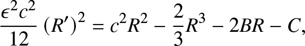(4.4)\begin{equation} \frac{\epsilon^{2}c^{2}}{12}\left(R'\right)^{2} = c^{2}R^{2} - \frac{2}{3}R^{3} - 2BR - C, \end{equation}

where we renamed the two constants of integration $\left(a,b\right) = \left(B,C\right)$.

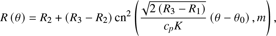
Note, in contrast to the previous case, this ODE has three free parameters $(B,C,c)$. A direct integration of Eq. (4.4) yields

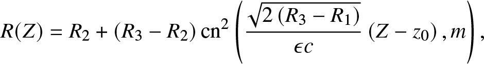(4.5)\begin{equation} R(Z) = R_{2} + \left(R_{3}-R_{2}\right)\text{cn}^{2}\left( \frac{\sqrt{2\left(R_{3}-R_{1}\right)}}{\epsilon c}\left(Z-z_{0}\right), m\right), \end{equation}

where $R_1 \lt R_2 \lt R_3$ denote the three roots of the potential $P(R) = -R^{3}+\frac{3}{2}c^{2}R^{2}-3BR-\frac{3}{2}C$, and

(4.6)\begin{equation} m = \frac{R_3 - R_2}{R_3 - R_1}. \end{equation}

Moreover, we can also deduce the leading-edge soliton amplitude through the periodic solution expression in (A.12). Namely, at the solitonic limit m → 1, so $R_2 \to R_1$ and the periodic solution reduces to the hyperbolic secant function with background given by R ₂ and amplitude denoted by $a^{+}$,

(4.7)\begin{equation} a^{+} = R_3 - R_2. \end{equation}

It will be convenient to express the soliton amplitude in terms of the wave’s background, which we call $r^+$, instead of the two unknown parameters R ₃ and R ₂. As we will see later in Sec. 7, $r^+$ represents the right value of the strain in the Riemann problem involving a jump from $r^{-}$ to $r^{+}$ (see also Eq. (2.4)). Since at the soliton limit $R_2 = R_1$ and since $R_2 = r^{+}$ is the background, we have that $R_1=R_2 = r^{+}$. On the other hand, to determine the unknown parameter R ₃, we expand the polynomial product $\left(R_1-R\right)\left(R_2-R\right)\left(R_3 - R\right)$ and then equate coefficients with the polynomial of $P\left(R\right)$ to obtain that

(4.8)\begin{equation} R_1 + R_2 + R_3 = \frac{3}{2}c^{2}, \end{equation}

where c denotes the theoretically predicted speed. Given that $R_1 = R_2 = r^{+}$, we solve for R ₃ in terms of $R_1, R_2$ and c and finally substitute it into Eq. (4.7) to arrive at the following explicit formula for the soliton amplitude,

(4.9)\begin{equation} a^{+} = \frac{3}{2}c^{2} - 3r^{+}. \end{equation}

4.3. Case p = 3

For the case p = 3, we first rewrite the travelling ODE as follows,

(4.10)\begin{equation} \left(R'\right)^{2} = -\frac{6}{\epsilon^{2}c^{2}}\left(R^{4}-2c^{2}R^{2}+4aR+2b\right) = -\frac{6}{\epsilon^{2}c^{2}}\left(R-R_1\right)\left(R-R_2\right)\left(R-R_3\right)\left(R-R_4\right). \end{equation}

We denote

(4.11)\begin{equation} \mu = -\frac{6}{\epsilon^{2}c^{2}}. \end{equation}

Clearly µ < 0, and then we first make the assumption that all four roots of $R_1, R_2, R_3, R_4$ are real valued and further assume the following order of the four roots,

(4.12)\begin{equation} R_1 \leq R_2 \leq R_3 \leq R_4, \end{equation}

and we assume that the oscillation occurs in the interval $R_3 \leq R \leq R_4$. Integration of Eq. (4.10) then yields

(4.13)\begin{equation} R = R_3 + \frac{\left(R_4 - R_3\right)\text{cn}^{2}\left(\zeta, m\right)}{1 + \frac{R_4 - R_3}{R_3 - R_1}\text{sn}^{2}\left(\zeta, m\right)}, \end{equation}

where

(4.14a)\begin{align} m &= \frac{\left(R_4 - R_3\right)\left(R_2 - R_1\right)}{\left(R_4 - R_2\right)\left(R_3 - R_1\right)}, \end{align}

(4.14b)\begin{align} \zeta &= \frac12{\sqrt{\left|\mu\right|\left(R_3 - R_1\right)\left(R_4 - R_2\right)}Z}. \end{align}

In the soliton limit where $R_3 \to R_2$, again by El et al. [Reference El, Hoefer and Shearer17], we obtain the following soliton solution:

(4.15)\begin{equation}R=R_2+\frac{R_4-R_2}{\text{cosh}^2\zeta+\frac{R_4-R_2}{R_2-R_1}\text{sinh}^2\zeta}.\end{equation}

Thus, we know immediately from the soliton solution (4.15) that the soliton amplitude reads

(4.16)\begin{equation}a^+=R_4-R_2,\end{equation}

which is completely analogous to the case of p = 2.

Finally, to get an explicit analytical formula for the soliton amplitude, we notice that by expanding the product of polynomials of (4.10) and equating the relevant coefficients, we have that

(4.17a)\begin{align} R_1 + R_2 + R_3 + R_4 &= 0, \end{align}

(4.17b)\begin{align} R_1R_2 + R_1R_3 + R_2R_3 + R_1R_4 + R_2R_4 + R_3R_4 &= -2c^{2}. \end{align}

Because we are at the soliton limit, we substitute the relation $R_3 = R_2$ into the system of (4.17a)-(4.17b) to obtain that

(4.18)\begin{align} R_1 + 2R_2 + R_4 &= 0, \end{align}

(4.19)\begin{align} 2R_1R_2 + R_2^{2} +R_1R_4 + 2R_2R_4 &= -2c^{2}. \end{align}

We then eliminate R ₁ from the system of (4.18)-(4.19) to have that

(4.20)\begin{equation} R_4^{2} + 2R_4R_2 + \left(3R_2^{2} - 2c^{2}\right) = 0. \end{equation}

The background is once again $R_2=r^{+}$. Then we solve (4.20) for R ₄ to obtain that

(4.21)\begin{equation} R_4^{\pm} = -R_2 \pm \sqrt{2\left(c^{2}-R_2^{2}\right)}. \end{equation}

Here, we need to take the root $R_4^{+}$ and ignore $R_4^{-}$ to avoid the issue of negative soliton amplitude. Finally, substituting $R_4^{+}$ into Eq. (4.16) we obtain an explicit soliton amplitude formula for p = 3,

(4.22)\begin{equation} a^{+} = \sqrt{2\left(c^{2} - \left(r^{+}\right)^{2}\right)} - 2r^{+}. \end{equation}

5. Conservation laws

Recall that the continuum model (2.12) is an approximation of the discrete granular chain at the level of the strain. Interestingly, this continuum model can be transformed into its associated displacement version which is an approximation model for the discrete system (2.1). Denoting the displacement variable for the PDE $u(X,T)$, the relationship between the displacement $u(X,T)$ and the strain $r(X,T)$ is

(5.1)\begin{equation} r(X,T) = u_X(X,T). \end{equation}

which then in turn would approximate the displacement of the granular chain via $u_n(t) \approx -\epsilon^{-1} u(X,T)$. Note that we need to include the negative sign since the strain variable is $r_n = u_{n-1}-u_{n}$, which has the opposite sign of the difference as compared to the one associated to the spatial derivative.

To obtain the continuum model in terms of $u(X,T)$, we substitute (5.1) into the original continuum model (2.12) and then observe that

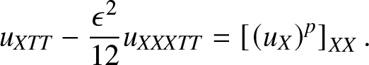(5.2)\begin{equation} u_{XTT} - \frac{\epsilon^{2}}{12}u_{XXXTT} = \left[\left(u_X\right)^{p}\right]_{XX}. \end{equation}

Integrating Eq. (5.2) with respect to X (assuming the integration constant to be zero) gives

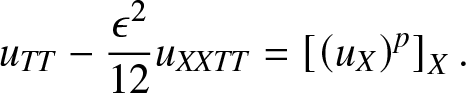(5.3)\begin{equation} u_{TT} - \frac{\epsilon^{2}}{12}u_{XXTT} = \left[\left(u_X\right)^{p}\right]_{X}. \end{equation}

Interestingly, the displacement continuum model (5.3) has a few conservation laws, namely the conservation of momentum and the conservation of energy. These two conservation laws can be seen by the following two rearrangements of Eq. (5.3),

(5.4)\begin{equation} \left(u_{X}u_{T}+\frac{\epsilon^{2}}{12}u_{XT}u_{XX}\right)_{T} - \left(\frac{1}{2}\left(u_{T}\right)^{2}+\frac{\epsilon^{2}}{24}\left(u_{XT}\right)^{2}+\frac{p}{p+1}\left(u_{X}\right)^{p+1}+\frac{\epsilon^{2}}{12}u_{XTT}u_{X}\right)_{X} = 0. \end{equation}

and

(5.5)\begin{equation} \left(\frac{1}{2}\left(u_{T}\right)^{2}+\frac{\epsilon^{2}}{24}\left(u_{XT}\right)^{2}+\frac{1}{p+1}\left(u_{X}\right)^{p+1}\right)_{T} - \left(\frac{\epsilon^{2}}{12}u_{XTT}u_{T}+\left(u_{X}\right)^{p}u_{T}\right)_{X} = 0, \end{equation}

respectively. We notice that Eq. (5.4) corresponds to the conservation of linear momentum, while Eq. (5.5) refers to the conservation of energy. In addition, it is also worthwhile to note that for the particular case when ϵ = 0 and p = 1, Eq. (5.3) simply reduces to the familiar linear wave equation which immediately falls back to a standard exercise regarding the two conservation laws (see, e.g., Strauss [Reference Strauss46]).

At the strain level, the PDE (2.12) yields an equivalent conservation law to (5.3):

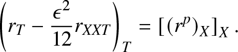(5.6)\begin{equation} \left(r_{T} - \frac{\epsilon^{2}}{12}r_{XXT}\right)_{T} = \left[\left(r^{p}\right)_{X}\right]_{X}. \end{equation}

The above conservation laws can be used to derive the Whitham modulation equations (e.g., see El and Hoefer [Reference El and Hoefer16]), but in the following section we will use an alternative approach based on Lagrangian formulation of the PDE (2.12).

6. Whitham modulation equations

Ever since the seminal work of Whitham Whitham [Reference Whitham51]; [Reference Whitham52] and of Gurevich and Pitaevskii Gurevich and Pitaevskii [Reference Gurevich and Pitaevskii21], the method of Whitham modulation theory has proved to be an effective tool for characterizing DSWs quantitatively (e.g., see El and Hoefer [Reference El and Hoefer16] for a review of this subject). The main object of study in Whitham modulation theory is the derivation of the so-called Whitham modulation equations, which govern spatio-temporal modulations of the periodic solutions of the model in question. In this section, we derive the Whitham modulation equations for the PDE (2.12) that approximates the granular chain in the continuum limit.

6.1. Theoretical preliminaries

The idea of modulation theory is to consider slow modulations of the parameters that completely determine the periodic solutions and derive their associated governing equations. To this end, we first introduce the wavenumber K and frequency Ω to rewrite the travelling-wave ansatz as $r(X,T) = R(\theta)$, with the phase variable $\theta = (KX-\Omega T)/\epsilon$ where $\Omega = c_p K$, to express our periodic solutions. For example, in the case of p = 2, the periodic solution in terms of θ is,

(6.1)\begin{equation} R\left(\theta\right) = R_{2} + \left(R_{3}-R_{2}\right)\text{cn}^{2}\left( \frac{\sqrt{2\left(R_{3}-R_{1}\right)}}{{c_p}K}\left(\theta - \theta_0 \right), m\right), \end{equation}

where θ ₀ is an arbitrary constant of integration which will be set to zero in the following. Note that Eq. (6.1) is equivalent to the one shown in Eq. (4.4) when returning to the $r(X,T)$ variables (in particular, the roots $R_1,R_2,R_3$ are the same despite the change of variable from Z to θ).

We now rewrite the periodic solution (6.1) so that its period is fixed, i.e., is independent of the solution parameters, which is needed in the derivation of the modulation equations. To this end, we use the fact that the periodic solution oscillates between the two values $R_2 \lt R_3$, and observe that

(6.2)\begin{equation} 2\pi = \int_{0}^{2\pi} \text{d}\theta = 2\int_{R_2}^{R_3}\frac{dR}{R_{\theta}} = 2\int_{R_2}^{R_3}\frac{dR}{\sqrt{\frac{8}{K^{2}{c_p}^{2}}\left(R_1 - R\right)\left(R_2 - R\right)\left(R_3 - R\right)}} = \frac{2 c_pKK_m}{\sqrt{2\left(R_3 - R_1\right)}}, \end{equation}

where K_m is the complete elliptic integral of the first kind. Thus, we have

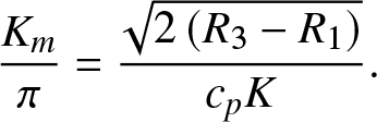(6.3)\begin{equation} \frac{K_m}{\pi} = \frac{\sqrt{2\left(R_3 - R_1\right)}}{c_pK}. \end{equation}

Using the independent variable θ as defined above, we then obtain that the periodic solution (6.1) is a 2π-periodic function

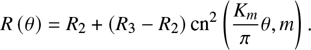(6.4)\begin{equation} R\left(\theta\right) = R_{2} + \left(R_{3}-R_{2}\right)\text{cn}^{2}\left(\frac{K_m}{\pi}\theta, m\right). \end{equation}

Furthermore, it is also convenient to reparametrize the solution, which is done by expressing the parameters $R_1,R_2, R_3$ in terms of $K,m,c_p$ using the following relations

(6.5a)\begin{align} &R_3 - R_1 = \frac{K^{2}c_p^{2}K_m^{2}}{2\pi^{2}}, \end{align}

(6.5b)\begin{align} &R_1 + R_2 + R_3 = \frac{3c_p^{2}}{2}, \end{align}

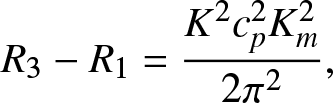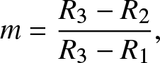(6.5c)\begin{align} &m = \frac{R_3 - R_2}{R_3 - R_1}, \end{align}

where (6.5a) comes from (6.3) and (6.5b) from the relation

(6.6)\begin{equation} (R_1 - R)(R_2 - R)(R_3 - R) = -R^{3} + \frac{3}{2}c_p^{2}R^{2} - 3BR -\frac{3}{2}C. \end{equation}

Then, solving the system (6.5) for $R_1, R_2, R_3$ in terms of $K,c_p,m$ yields

(6.7a)\begin{align} R_1 &= \frac{c_p^{2}}{2} + \frac{\left(m-2\right)K^{2}c_p^{2}K_m^{2}}{6\pi^{2}}, \end{align}

(6.7b)\begin{align} R_2 &= \frac{c_p^{2}}{2} + \frac{\left(1-2m\right)K^{2}c_p^{2}K_m^{2}}{6\pi^{2}}, \end{align}

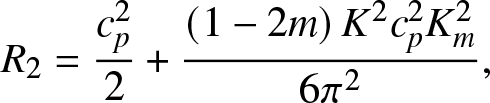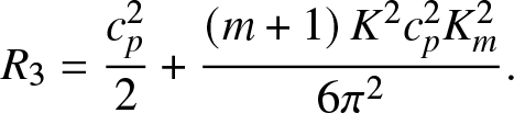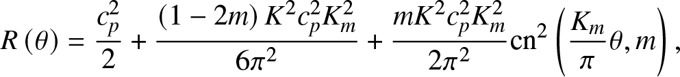
(6.7c)\begin{align} R_3 &= \frac{c_p^{2}}{2} + \frac{\left(m+1\right)K^{2}c_p^{2}K_m^{2}}{6\pi^{2}}. \end{align}

Substituting (6.7) into the reparametrized periodic solution (6.4) yields

(6.8)\begin{equation} R\left(\theta\right) = \frac{c_p^{2}}{2} + \frac{\left(1-2m\right)K^{2}c_p^{2}K_m^{2}}{6\pi^{2}} + \frac{mK^{2}c_p^{2}K_m^{2}}{2\pi^{2}}\text{cn}^{2}\left(\frac{K_m}{\pi}\theta, m\right), \end{equation}

where now clearly the periodic solution is parametrized by the three parameters $c_p, K, m$.

6.2. Derivation of modulation equations

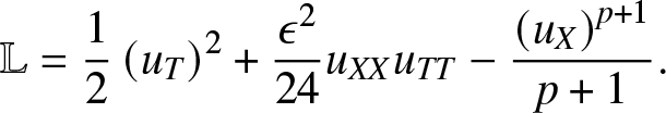
To derive the modulation equations, we will use the method of averaged Lagrangian Kamchatnov [Reference Kamchatnov31]. We first note that the PDE model in its displacement form, see Eq. (5.3), can be obtained through a variational principle. We observe that the Lagrangian density $\mathbb{L}$ associated with Eq. (5.3) is

(6.9)\begin{equation} \mathbb{L} = \frac{1}{2}\left(u_T\right)^{2} + \frac{\epsilon^{2}}{24}u_{XX}u_{TT} - \frac{\left(u_X\right)^{p+1}}{p+1}. \end{equation}

Equation (5.3) represents the Euler-Lagrange equation for the action functional $\iint\mathbb{L} \, dX dT$. It is worth noting that the middle term could be replaced by $(\epsilon^2/24)u^2_{XT}$, which could be interpreted as a “microkinetic energy” Theil and Levitas [Reference Theil and Valery48], although we will not pursue that hereafter.

A modulated travelling wave is an approximate solution whose parameters vary slowly relative to a fast phase $\theta(X,T)$ and a so-called fast pseudo phase $Q(X,T)$. The ansatz is formulated at the level of the displacement and has the form

(6.10)\begin{equation} u(X,T) = \epsilon\left( Q(X,T) + \psi\left( \theta(X,T) \right) \right), \end{equation}

where,

(6.11a)\begin{align} \theta_X = K(X,T)/\epsilon\,,\qquad \theta_T = - \Omega(X,T)/\epsilon\,, \end{align}

(6.11b)\begin{align} Q_X = \beta(X,T)/\epsilon\,,\qquad Q_T = - \gamma(X,T)/\epsilon\,, \end{align}

and where $\psi(\theta)$ a 2π-periodic function with zero average, namely $\overline{\psi} = 0$, where the bar denotes the averaging operation over a period of the function,

(6.12)\begin{equation} \overline{f} = \frac{1}{2\pi}\int_0^{2\pi}f\left(\theta\right)\,d\theta. \end{equation}

Note that, with this ansatz, all terms can be expressed in terms of the travelling wave at the strain level R. In particular, $R=R(\theta)$ satisfies

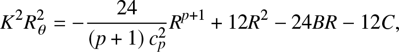(6.13)\begin{equation} K^{2}R_\theta^{2} = -\frac{24}{\left(p+1\right)c_p^{2}}R^{p+1} + 12R^{2} - 24BR - 12C, \end{equation}

where $c_p = \Omega/K$ and $B, C$ are two constants of integration. Equation (6.13) is analogous to Eq. (4.4), but the ϵ has vanished due to the scaling of θ. Note that $R(\theta)$ relates to $u(X,T)$ and its derivatives in the following way,

(6.14a)\begin{align} u_X &= \beta + \psi'(\theta) K = R(\theta) \end{align}

(6.14b)\begin{align} u_T &= -\gamma - \psi'(\theta)\Omega = -\gamma - (R(\theta) - \beta)c_p \end{align}

(6.14c)\begin{align} u_{XX} &= \psi''(\theta)K^2/\epsilon = R_\theta(\theta)K/\epsilon \end{align}

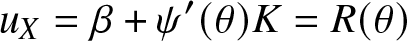(6.14d)\begin{align} u_{TT} &= \psi''(\theta)\Omega^2/\epsilon = R_\theta(\theta) \Omega^2/( K \epsilon) \end{align}

where we have used Eq. (6.11). Now we are ready to derive modulation equations. Substituting (6.10) into the Lagrangian density of Eq. (6.9) and expressing everything in terms of R using Eqs. (6.13) and (6.14) yields

(6.15)\begin{equation} \mathbb{L} = \frac{\Omega^{2}}{12}\left(R_\theta\right)^{2} +\left(-\beta c_p^{2}+\gamma c_p + Bc_p^{2}\right)R + \frac{1}{2}\gamma^{2}+\frac{1}{2}c_p^{2}\beta^{2}-\beta\gamma c_p + \frac{1}{2}Cc_p^{2}. \end{equation}

The method of the averaged Lagrangian assumes that the wave parameters are constant over one period of motion. We therefore compute the average Lagrangian,

(6.16)\begin{equation} \mathcal{L} = \frac{1}{2\pi}\int_{0}^{2\pi}\mathbb{L}\,d\theta = \frac{\Omega c_p}{12}W\left(B,C,c_p\right)+\frac{1}{2}\gamma^{2}-\frac{1}{2}c_p^{2}\beta^{2}+\frac{1}{2}Cc_p^{2}+\beta Bc_p^{2}, \end{equation}

where we have the “action” integral $W\left(B,C,c_p\right)$ defined as follows

(6.17)\begin{equation} W\left(B,C,c_p\right) = \frac{K}{2\pi} \int_{0}^{2\pi}\left(R_\theta\right)^{2}d\theta = \frac{1}{2\pi}\oint\left(-\frac{24}{\left(p+1\right)c_p^{2}}R^{p+1}+12R^{2}-24BR - 12C\right)^{1/2}dR. \end{equation}

The modulation system then simply follows from the average variational principle,

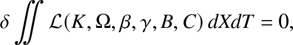(6.18)\begin{equation} \delta \iint \mathcal{L}(K,\Omega ,\beta,\gamma, B, C)\, dXdT = 0, \end{equation}

which then yields the following Euler-Lagrange equations (and corresponding consistency relations),

(6.19a)\begin{align} &\mathcal{L}_B = 0, \qquad \mathcal{L}_C = 0, \end{align}

(6.19b)\begin{align} &\frac{\partial}{\partial T}\mathcal{L}_\Omega -\frac{\partial}{\partial X}\mathcal{L}_K = 0, \qquad K_{T} + \Omega_{X} = 0, \end{align}

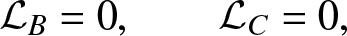(6.19c)\begin{align} &\frac{\partial}{\partial T}\mathcal{L}_\gamma - \frac{\partial}{\partial X}\mathcal{L}_\beta = 0, \qquad \beta_{T} + \gamma_{X} = 0\,. \end{align}

Using equations (6.16), we obtain from (6.19a) that

(6.20a)\begin{align} &\beta = -\frac{\Omega}{12c_p}W_B \end{align}

(6.20b)\begin{align} &\frac{\Omega c_p}{12}W_C + \frac{1}{2}c_p^{2} = 0. \end{align}

Equation (6.20a) simplifies to

(6.21)\begin{equation} \beta = \overline{R}, \end{equation}

which simply states the average of the strain profile of the wave is β, a fact that is obvious by the construction of the ansatz Eq. (6.10). For Eq. (6.20b), if we solve for the wavenumber K, we end up with

(6.22)\begin{equation} K = -\frac{6}{W_C}. \end{equation}

Then, the nonlinear dispersion relation reads

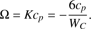(6.23)\begin{equation} \Omega = Kc_p = -\frac{6c_p}{W_C}. \end{equation}

We observe that the two equations of (6.21) and (6.22) reduce the original set of six parameters now to only four independent parameters, and this further indicates that the four equations in (6.19b) and (6.19c) finally yield a closed modulation system.

Equation (6.19c) can be written as

(6.24a)\begin{align} \gamma_{T}-\left(-c_p^{2}\beta + Bc_p^{2}\right)_{X} &= 0, \end{align}

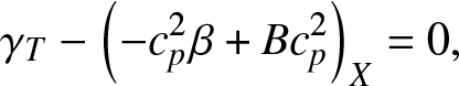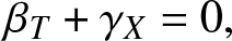(6.24b)\begin{align} \beta_{T} + \gamma_{X} &= 0, \end{align}

whereas Eq. (6.19b), can be written as

(6.25a)\begin{align} \left(\frac{c_p}{12}\left(2W + c_pW_{c_p}\right) + \frac{2c_p}{K}\left(-\frac{1}{2}\beta^{2}+\frac{1}{2}C+\beta B\right)\right)_{T} \kern10em & \nonumber\\ + \left(\frac{c_p^{2}}{12}\left(W_{c_p}c_p + W\right) + \frac{2c_p^{2}}{K}\left(-\frac{1}{2}\beta^{2}+\frac{1}{2}C+\beta B\right)\right)_{X} &= 0, \end{align}

(6.25b)\begin{align} K_{T} + \Omega_{X} &= 0. \end{align}

Taken together, the four equations in Eqs. (6.24a)-(6.25b) form a closed system of modulation equations for the periodic solutions of the continuum model. One should also note that we expect that if the alternative strategy of averaging the conservation laws is applied, an equivalent Whitham modulation system will be obtained. However, since the conservation laws for the PDE model under consideration are formulated in terms of displacements rather than strains, we do not explore this approach further.

7. Riemann problems and DSW fitting

In this section, we discuss the setup of the Riemann problems for both the continuum PDE and the discrete granular DDE, as well as offer a comparison of the two.

7.1. Riemann invariants of the dispersionless system

Before discussing numerical simulations and the analytical method of DSW fitting, we need to understand the dispersionless averaged version of the continuum model (2.12). First note that Eq. (2.12) can be written in the following form,

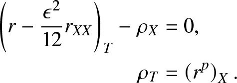(7.1)\begin{equation} \begin{aligned} \left(r - \frac{\epsilon^{2}}{12}r_{XX}\right)_{T} - \rho_{X} &= 0,\\ \rho_{T} &= \left(r^{p}\right)_{X}. \end{aligned} \end{equation}

According to El [Reference El14], the Whitham modulation equations at both harmonic and solitonic edges should read

(7.2a)\begin{align} \left(\overline{r}\right)_T - \overline{\rho}_X &= 0, \end{align}

(7.2b)\begin{align} \overline{\rho}_T - \left[\left(\overline{r}\right)^{p}\right]_X &= 0. \end{align}

These equations are obtained by setting the dispersion term to zero (ϵ = 0) in Eq. (7.1) and averaging. We can then further put the first-order system (7.2) into the associated characteristic form which reads

(7.3a)\begin{align} \frac{\partial {q_1}}{\partial T}+p^{\frac{1}{2}}\overline{r}^{\frac{p-1}{2}}\frac{\partial {q_1}}{\partial X} &= 0, \end{align}

(7.3b)\begin{align} \frac{\partial {q_2}}{\partial T} - p^{\frac{1}{2}}\overline{r}^{\frac{p-1}{2}}\frac{\partial {q_2}}{\partial X} &= 0, \end{align}

where the two Riemann invariants are

(7.4a)\begin{align} {q_1} &= \overline{\rho} - \frac{2p^{\frac{1}{2}}}{p+1}\overline{r}^{\frac{p+1}{2}}, \end{align}

(7.4b)\begin{align} {q_2} &= \overline{\rho} + \frac{2p^{\frac{1}{2}}}{p+1}\overline{r}^{\frac{p+1}{2}}. \end{align}

which are associated with the two characteristic velocities $\lambda_{+} = p^{\frac{1}{2}}\overline{r}^{\frac{p-1}{2}}$ and $\lambda_{-} = -p^{\frac{1}{2}}\overline{r}^{\frac{p-1}{2}}$, respectively.

7.2. Initial data for the continuum model

The classic Riemann problem for the continuum model corresponds to the initial conditions

(7.5)\begin{equation} r(X,0) = \begin{cases} r^{-}\,, & X \lt 0\,,\\ r^{+}\,, & X \gt 0\,, \end{cases} \qquad \rho(X,0) = \begin{cases} \rho^{-}\,, & X \lt 0\,,\\ \rho^{+}\,, & X \gt 0\,. \end{cases} \end{equation}

These initial conditions are assumed when conducting the DSW fitting analysis in Sec. 7.5. In what follows, we assume that $r_- \gt r_+$.

The initial condition for the variable ρ should satisfy a jump condition, as detailed in El [Reference El14]. In particular, this jump condition is obtained by demanding that the Riemann invariant ${q_2}$ (with associated characteristic velocity $\lambda_{-}$) of the dispersionless system Eq. (7.2) to be constant. In other words, we must have that

(7.6)\begin{equation} {q_2}\left(r^{+},\rho^{+}\right) = {q_2}\left(r^{-},\rho^{-}\right). \end{equation}

Notice that the values of ρ ⁻ and $\rho^{+}$ are not known at this point, and we have to determine their values according to the jump condition specified in Eq. (7.6). To this end, substituting the expression of ${q_2}$ defined in Eq. (7.4) into the jump condition (7.6), we obtain that,

(7.7)\begin{equation} \rho^{-} + \frac{2\sqrt{p}}{p+1}(r^{-})^{\frac{p+1}{2}} = \rho^{+} + \frac{2\sqrt{p}}{p+1}(r^{+})^{\frac{p+1}{2}}. \end{equation}

If considering step initial data, as defined in Eq. (7.8), one can freely select $r^+,r^-,\rho^+$ and then ρ ⁻ is determined via Eq. (7.7).

For numerical simulations, we will employ a spectral method to discretize the spatial variables, and thus we require initial conditions that will respect the periodic boundary conditions. The following “box-type” initial data are one such choice and are analogous to Eq. (7.5),

(7.8)\begin{equation} r(X,0) = \begin{cases} r^{-}\,, & a \lt X \lt b\,,\\ r^{+}\,, & X \lt a~\vee~ X \gt b\,, \end{cases} \qquad \rho(X,0) = \begin{cases} \rho^{-}\,, & a \lt X \lt b\,,\\ \rho^{+}\,, & X \lt a~\vee~ X \gt b\ \end{cases} \end{equation}

where $a,b\in\mathbb{R}$ are two real constants with (a < b). The discontinuity in this initial data, however, makes it less desirable for computations. Thus, for the numerical approximation of the PDEs, we employ a smooth approximation of the “box-type” initial strain,

(7.9)\begin{equation} r(X,0) = r^{+} - \frac{r^{+} - r^{-}}{2}\left(\text{tanh}\left(50\left(X-a\right)\right) - \text{tanh}\left(50\left(X - b\right)\right)\right). \end{equation}

We now need to find an appropriate smooth approximation of $\rho(X,0)$ that is consistent with Eq. (7.8) and that satisfies the jump conditions Eq. (7.7). Assuming $r^+,r^-,\rho^+$ are fixed (for which the nature of the equations allows the freedom to arbitrarily select), and based on the jump condition of Eq. (7.7), we take the following initial condition for the variable ρ,

(7.10)\begin{equation} \rho(X,0) = \frac{2\sqrt{p}}{p+1}\left(\left(r^{+}\right)^{\frac{p+1}{2}} - r\left(X,0\right)^{\frac{p+1}{2}}\right) + \rho^{+}. \end{equation}

This further suggests that the value of ρ ⁻ is given as follows,

(7.11)\begin{equation} \rho^{-} = \frac{2\sqrt{p}}{p+1}\left(\left(r^{+}\right)^{\frac{p+1}{2}} - \left(r^{-}\right)^{\frac{p+1}{2}}\right) + \rho^{+}, \end{equation}

which is clearly consonant with the jump condition Eq. (7.7). With $r_- \gt r_+$ and $\rho(X,0)$ chosen according to Eq. (7.7), a right-moving DSW will form on the right of the “box”, whereas a left-moving rarefaction wave will form on the left of the “box”. Since our focus is on the formation of DSWs, we do not report results on the rarefaction waves. See Secs. 7.4 and 8 for examples of right-moving DSWs.

If one were to demand that the Riemann invariant q ₁ be fixed (rather than q ₂) the jump condition Eq. (7.7) would become

(7.12)\begin{equation} \rho^{-} - \frac{2\sqrt{p}}{p+1}(r^{-})^{\frac{p+1}{2}} = \rho^{+} - \frac{2\sqrt{p}}{p+1}(r^{+})^{\frac{p+1}{2}}. \end{equation}

It is worth noting that a choice of $r_- \gt r_+$ and $\rho(X,0)$ to satisfy this jump condition would lead to a left-moving DSW on the left of the “box” and a rarefaction wave moving to the right. The results are qualitatively similar to the case with q ₂ fixed, and so this setting is not discussed further herein.

7.3. Initial data for the discrete model

To set up the Riemann problem for the original granular DDE that is consistent with the initial data we just discussed we need to further understand how the density variable ρ relates to the discrete variables. To this end, we consider an alternative first-order form of our continuum PDE which has a direct connection to the lattice system. In particular, we observe that instead of rewriting the continuum model as Eq. (7.1), it can also be written as follows,

(7.13a)\begin{align} r_T &= v_X, \end{align}

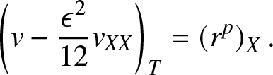(7.13b)\begin{align} \left(v - \frac{\epsilon^{2}}{12}v_{XX}\right)_T &= \left(r^{p}\right)_X. \end{align}

Here, $r(X,T)$ still represents an approximation of the strain of the lattice r_n, but $v(X,T)$ is related to the particle velocity, $\dot{u}_n$. So now both variables of the PDE formulation are directly related to physical variables of the granular chain. We then notice that, by setting $\rho = v - \frac{\epsilon^{2}}{12}v_{XX}$, the system (7.13) is equivalent to (7.1). This gives an interpretation of ρ in terms of the physical variables of the granular chain (namely in terms of the particle velocity).

If we denote the initial conditions of Eq. (7.1) as

(7.14a)\begin{align} r\left(X,0\right) &= f(X), \end{align}

(7.14b)\begin{align} \rho\left(X,0\right) &= g(X) \end{align}

then the associated initial conditions for the system (7.13) read

(7.15a)\begin{align} r\left(X,0\right) &= f(X), \end{align}

(7.15b)\begin{align} v\left(X,0\right) &= \mathcal{F}^{-1}\left[\frac{\mathcal{F}\left[g(X)\right]}{1 + \frac1{12}{\epsilon^{2}K^{2}}}\right] = \int_{-\infty}^\infty h(X')g(X - X')\,dX'\,, \end{align}

where $\mathcal{F}^{-1}, \mathcal{F}$ refer to the inverse and usual Fourier operators, K the Fourier wave number, and

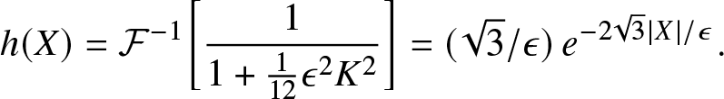(7.16)\begin{equation} h(X) = \mathcal{F}^{-1}\bigg[\frac1{1 + \frac1{12}{\epsilon^{2}K^{2}}}\bigg] = (\sqrt3/\epsilon)\,e^{-2\sqrt3|X|/\epsilon}. \end{equation}

Figure 3 showcases the profiles of the initial conditions in Eq. (7.15).

Now, we finally consider the Riemann problem of the granular DDE. First, we rewrite the second-order discrete system (2.2) as the following equivalent first-order discrete system,

(7.17a)\begin{align} \dot r_n &= s_n, \end{align}

(7.17b)\begin{align} \dot s_n &= r_{n+1}^{p} - 2r_n^{p} + r_{n-1}^{p}, \end{align}

where s_n is the strain derivative. Similar to the initial conditions in (7.14), the Riemann initial conditions for the discrete system (7.17) read

(7.18a)\begin{align} r_n(0) &= f\left(n\epsilon\right), \end{align}

(7.18b)\begin{align} s_n(0) &= v\left(n\epsilon, 0\right) - v\left(\left(n-1\right)\epsilon, 0\right), \end{align}

where the right-hand side v in Eq. (7.18) comes from the continuum ICs expressed in (7.14)(b).

Figure 3.

The initial conditions in Eqs. (7.14). The background and parameter values are $r^{-} = 1$, $r^{+} = 0.9$, p = 2, and ϵ = 0.1.

7.4. Numerical simulation and DSWs

Figure 4 displays the simulation of the Riemann problem for the DDE. A waveform emerges at the right upper corner of the “box-type” initial data. This waveform connects left state ( $r^-$) to the right state ( $r^+$) and expands as time increases. If one zooms into a small spatial-window of the waveform, it will appear as though the wave is periodic. The underlying parameters of the periodic wave will depend on where in the lattice you zoom, and hence the waveform is modulated. This is the so-called DSW. At the front of the wave (called the leading edge) the wave closely resembles a solitary wave, and it travels with a near constant speed $s^+$ and has some amplitude $a^+$. On the other hand, the back part of the DSW (called the trailing edge) is characterized by a linear wave with some wavenumber $k^-$ travelling at a speed $s^{-}$ with amplitude that vanishes as the trailing edge is approached from within the DSW. For any finite time snapshot of the DSW, there will be linear waves that are located around the background value of $r^{-}$. These linear waves are not a part of the DSW per se, and vanish for $t\rightarrow \infty$. To avoid any possible confusion, we point out that the PDE (2.12) is non-dispersive only for small-amplitude waves on a zero background. Conversely, it is fairly straightforward to see that the PDE does admit small-amplitude waves riding on top of any non-zero background, which is what we refer to with the term linear waves.

Figure 4(a) shows a time snapshot of the DSW, where the key elements of the DSW, namely the leading and trailing edge can be seen, along with the linear waves that are always present for any finite time snapshot. Figure 4(b) shows a plot of the strain magnitude $r(X,T)$ where the expanding oscillatory region (i.e., the DSW) can be seen. The dashed lines in panel (b) are analytical approximations of the leading and trailing edges that stem from the so-called DSW fitting method. Before discussing those approximations, we discuss some preliminaries involving the dispersionless system.

Figure 4.

Numerical simulation of the Riemann problem: The left panel shows the profile of the DSW of the continuum model (2.12) at T = 50, while the right panel depicts the plot of the strain magnitude $r(X,T)$, and the two black dashed lines in the density plot represent the leading (upper) and the trailing (lower) edges of the DSW, respectively. In particular, the upper and the lower dashed black lines depict $X = s^{+}T$ and $X = s^{-}T$ where $s^{+}, s^{-}$ are obtained based on Eqs. (7.23). Meanwhile, notice that the parameters of $r^{+}, r^{-}$ in the Riemann initial condition (7.8) are set to be $r^{+} = 0.8$, and $r^{-} = 1$ in the numerical simulation.

7.5. DSW fitting

Next, we consider special reductions of Whitham’s modulation system that we have derived in Sec. 6. These reductions will be used to obtain valuable information about the DSWs, such as the leading and trailing edge speeds as well as the amplitude of the solution at the leading edge of the DSW and the wavenumber at its trailing edge. To this end, we apply the well established, and highly successful in the continuum limit “DSW fitting” method of El [Reference El14], which remains relatively unexplored in the lattice setting.

We note that the applicability of the method requires the underlying modulation equations to be strictly hyperbolic and genuinely nonlinear, e.g., see El [Reference El14]; Lowman and Hoefer [Reference Lowman and Hoefer36]; Hoefer [Reference Hoefer27]. It is not known at present whether the modulation equations derived in Section 6 satisfy these requirements. On the other hand, we will proceed under the assumption that these conditions are satisfied, and we will validate the calculations a posteriori by comparing the theoretical predictions with the results of direct numerical simulations of the PDE (2.12) and the original DDE (2.2), demonstrating good agreement.

One preliminary and important task is to compute the associated linear dispersion relation of the original continuum model (2.12). Leveraging our earlier analysis in Eq. (2.13), we recall that the linear dispersion relation reads:

(7.19)\begin{equation} \Omega_0^2(A,K) = {pA^{p-1}K^2} \bigg/ \bigg( 1+\frac{\epsilon^2}{12}K^2 \bigg). \end{equation}

Then, in line with the general DSW fitting theory of El [Reference El14], the trailing-edge wave number $K^{-}$ and the leading-edge conjugate wave number $\widetilde{K}^{+}$ have to satisfy the following two boundary value problems,

(7.20a)\begin{align} \frac{dK}{d\overline{r}} &= \frac{\partial\Omega_0/\partial\overline{r}}{\lambda_{+}\left(\overline{r}\right) - \partial\Omega_0/\partial K}, \qquad K(r^{+}) = 0, \end{align}

(7.20b)\begin{align} \frac{d\widetilde{K}}{d\overline{r}} &= \frac{\partial \widetilde{\Omega}_s/\partial\overline{r}}{\lambda_{+}\left(\overline{r}\right) - \partial\widetilde{\Omega}_s/\partial\widetilde{K}}, \qquad \widetilde{K}(r^{-}) = 0, \end{align}

where $r^{+}, r^{-}$ refer to the two background values of the strain in the Riemann initial condition (defined in Eq. (7.8)) representing a jump from $r^{-}$ to $r^{+}$. We further notice that the notation $\widetilde{\Omega}_s$ represents the conjugate linear dispersion relation which is determined according to the prescription of El [Reference El14] as:

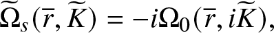(7.21)\begin{equation} \begin{aligned} \widetilde{\Omega}_s(\overline{r},\widetilde{K}) = -i\Omega_0(\overline{r},i\widetilde{K}), \end{aligned} \end{equation}

where the linear dispersion relation Ω₀ is given in (7.19).

A direct integration of both ODEs in (7.20) with the help of the boundary conditions yields the following two transcendental equations which are used to determine the numerical values of trailing-edge wavenumber and of the leading edge conjugate wavenumber,

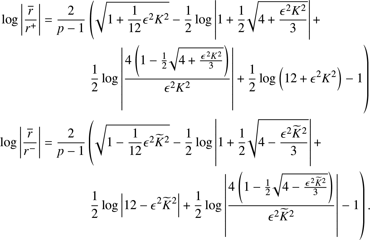(7.22)\begin{equation} \begin{aligned} \log\left|\frac{\overline{r}}{r^{+}}\right| = \frac{2}{p-1}&\left(\sqrt{1+\frac{1}{12}\epsilon^{2}K^{2}} - \frac{1}{2}\log\left|1 + \frac{1}{2}\sqrt{4 + \frac{\epsilon^{2}K^{2}}{3}}\right| + \right. \\ &\left. \frac{1}{2}\log\left|\frac{4\left(1-\frac{1}{2}\sqrt{4+\frac{\epsilon^{2}K^{2}}{3}}\right)}{\epsilon^{2}K^{2}}\right| + \frac{1}{2}\log\left(12 + \epsilon^{2}K^{2}\right) - 1\right) \\\log\left|\frac{\overline{r}}{r^{-}}\right| = \frac{2}{p-1}&\left(\sqrt{1-\frac{1}{12}\epsilon^{2}\widetilde{K}^{2}} - \frac{1}{2}\log\left|1+\frac{1}{2}\sqrt{4-\frac{\epsilon^{2}\widetilde{K}^{2}}{3}}\right|+\right.\\ &\left.\frac{1}{2}\log\left|12-\epsilon^{2}\widetilde{K}^{2}\right|+\frac{1}{2}\log\left|\frac{4\left(1-\frac{1}{2}\sqrt{4-\frac{\epsilon^{2}\widetilde{K}^{2}}{3}}\right)}{\epsilon^{2}\widetilde{K}^{2}}\right| - 1\right). \end{aligned} \end{equation}

To compute numerically the trailing-edge wavenumber and the leading-edge conjugate wavenumbers, we first notice that all the parameters in Eq. (7.22) are known except K and $\widetilde{K}$ which are the target unknown variables to be sought. To obtain the latter, we observe that at the trailing and leading edges, $\overline{r} = r^{-}$ and $\overline{r} = r^{+}$, respectively. We then substitute all the known parameters in Eq. (7.22) to solve for K and $\widetilde{K}$.

In addition, the trailing and leading edge speeds, denoted by $s^{-}$ and $s^{+}$, respectively, can be computed using the following formulas of the DSW fitting method:

(7.23a)\begin{align} s^{-} &= \frac{\partial\Omega_0}{\partial K}\left(r^{-}, K^{-}\right) = \frac{p^{\frac{1}{2}}\left(r^{-}\right)^{\frac{p-1}{2}}}{\left(1 + \frac{1}{12}\left(\epsilon K^{-}\right)^{2}\right)^{\frac{3}{2}}}, \end{align}

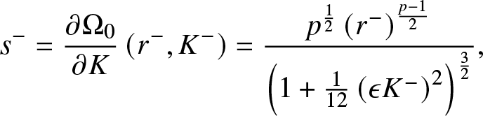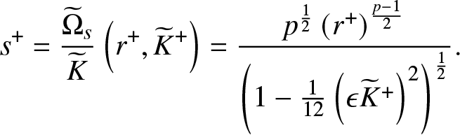(7.23b)\begin{align} s^{+} &= \frac{\widetilde{\Omega}_s}{\widetilde{K}}\left(r^{+}, \widetilde{K}^{+}\right) = \frac{p^{\frac{1}{2}}\left(r^{+}\right)^{\frac{p-1}{2}}}{\left(1 - \frac{1}{12}\left(\epsilon\widetilde{K}^{+}\right)^{2}\right)^{\frac{1}{2}}}. \end{align}

An important observation here is that in expression (7.22) and (7.23), there is only a single effective parameter $\epsilon K$. This implies that once we return to the original granular variables and compare the wavenumber prediction of the DSW fitting and the wavenumber corresponding to the lattice, the prediction once again will be independent of ϵ, in light of the relationship $k = \epsilon K$. The same is true for the leading and trailing edge speeds, namely they are independent of ϵ, much like the case of the solitary waves, whose predictions were also independent of ϵ. Finally, we recall that we can also compute the analytical prediction for the soliton amplitude for the cases of $p = 2, 3$ by using the formulas in Eq. (4.9) and Eq. (4.22), respectively, with replacing c by $s^{+}$ in Eqs. (7.23).

8. Numerical validation

We are now ready to validate the theoretical results obtained previously by numerically solving the Riemann problems and comparing the numerical results with the associated quantities derived from the DSW fitting method. We employed a fourth-order Runge-Kutta method for time stepping both the discrete model (2.2) and the quasi-continuum PDE (2.12), as well as pseudo-spectral methods to discretize the spatial derivatives in Eq. (2.12).

Firstly we present the DSW profiles comparison as shown in the following figures for the cases of p = 3 and p = 2, respectively. Note that the smallness parameter ϵ is set to be 0.1 over all PDE simulations. To make a direct comparison between the DSWs obtained from the PDE and DDE simulations, when the spatial variable of the PDE simulation is taken to be X, we consistently define the DDE spatial variable to be $n\epsilon$ per the principal relationship between the PDE and DDE spatial domains $X = n\epsilon$.

Figure 5 shows the granular lattice subject to the Riemann initial data given by Eq. (7.18) with $r^-=1$ and $r^+=0.95$ (see the red dots). Only a zoom of the right-moving wave is shown, which is where the DSW appears. The solid blue lines are the numerical simulation of the regularized continuum PDE proposed herein, namely Eq. (2.12) with the consistent initial data given by Eqs. (7.9) and  (7.10). The lattice and PDE simulations agree very well. The solid black lines represent the approximations obtained from the DSW fitting method described previously. In particular for panel (a), the vertical lines represent the trailing and leading edges, namely, $60 s^-$ and $60 s^+$, respectively, where t = 60 is the time chosen and $s^-,s^+$ are the speeds from Eqs. (7.23). The sloped lines are an approximation of the envelope, and were obtained by connecting the point $(60 s^-,r^-)$ with $(60 s^+, a^+ + r^+)$ (the top line) and the line defined by the points $(60 s^-,r^-)$ with $(60 s^+, r^+)$, (the bottom line). Panel (b) is similar but the time t = 150 is used in place of t = 60. The lattice simulations are encompassed by the triangle enclosed by the solid lines demonstrating that the theoretical prediction of the DSW characteristics (based on the DSW fitting discussed above) agrees quite well with the numerical observations.

Such a quantitatively adequate fitting (everywhere but for part of the DSW’s linear tail) also indicates that the proposed PDE model (2.12) succeeds in characterizing the DSW embedded in the discrete model. The inaccuracy at the tail is common when approximating DSWs El et al. [Reference El, Hoefer and Shearer17]. While the linear tails decay in time (with the rate $t^{-1/3}$) Mielke and Patz [Reference Alexander and Carsten3] it will always be present in any finite simulation.

Figure 5.

Comparison of the DSW profiles for the cases of p = 3 and p = 2: in both left and right panels, the blue solid curves represent the DSW simulated from the regularized continuum PDE model (2.12), and the red dots refer to the DSW of the DDE simulation. The black triangular envelope denotes the theoretical DSW fitting. Notice that the initial condition for the strain variable r is given in Eq. (7.9) where $a = 200, b = 500$, and the background information is given by $r^{+} = 0.95, r^{-} = 1$. The corresponding initial condition for the density ρ is given in Eq. (7.10), and the computational domain is $X \in \left[0, 1000\right]$. Notice that the left panel refers to the evolution at T = 60 (for the PDE (2.12)) and t = 600 (for the DDE (2.2)), while the right panel denotes the evolution dynamics at T = 150 (for the PDE (2.12)) and t = 1500 (for the DDE (2.2)).

As an aside, it is worth mentioning that we have also simulated the models of Ahnert and Pikovsky [Reference Ahnert and Pikovsky2] (i.e., Eq. (2.9)) and Nesterenko [Reference Nesterenko39] (i.e., Eq. (3.11)) for the Riemann problem initial conditions of the present work. In line with the expectation associated with their dispersion relation discussed earlier, we have found that while these models form a DSW, the latter keeps increasing in amplitude indefinitely as a result of the ultraviolet catastrophes present in the models. This corroborates our expectation that such models, while meaningful towards a travelling or periodic wave analysis, cannot be used for the initial value problem considered herein.

To further quantify the fitting of the DSWs, especially in connection to the theoretical predictions, we compute numerically some important quantities relevant to the DSWs including (i) leading-edge speeds, (ii) leading-edge soliton amplitudes, (iii) trailing-edge speeds and (iv) trailing-edge wavenumbers. Before we display the numerical results of the four quantities, we first discuss the method applied to measure these quantities in the numerical simulation. For the leading-edge calculations including items (i) and (ii), we pinpoint the location of the leading-edge as the x coordinate of the highest peak of the DSW. We then compute the leading-edge speed by first recording the leading-edge locations at various times t. From this set of data we find the best-fit line and use the corresponding slope as the prediction for the leading-edge speed. On the other hand, for the numerical leading-edge soliton amplitudes denoted by $a^{+}$, it can be computed numerically via the following formula,

(8.1)\begin{equation} a^{+} = \max_{X}\{u\left(X,T_f\right)\} - r^{+}, \end{equation}

where $u\left(X,T_f\right)$ is the numerical solution to the PDE/DDE models at the final time of the simulation $t = T_f$. Moreover, for the theoretical leading-edge soliton amplitudes, we compute them by applying the formulas (4.9) and (4.22) for the cases of p = 2 and p = 3, respectively. Next, for the trailing-edge computation, to identify the trailing-edge location needed for (iii) and (iv), we find the best fit line passing through a set of local maxima (which set is described below) and a best fit line passing through a set of local minima. Similar to the sloped lines of Fig. 5, these two lines will intersect. That intersection point will act as measurement of the numerical trailing edge. In order to find a suitable interval of maxima (and minima) we first define the quantities

(8.2a)\begin{align} a^{u} &= r^{-} + \frac{\left|r^{-} - r^{+}\right|}{N}, \end{align}

(8.2b)\begin{align} a^{l} &= r^{-} - \frac{\left|r^{-} - r^{+}\right|}{N}, \end{align}

where $N\in\mathbb{Z}$ is a positive integer. For example, N = 4, 5 are utilized in our numerical simulations. These values are approximately $3/4$ and $1/4$ the amplitude of the DSW, respectively. Then, the sets of local maxima and minima are those with values that fall in the intervals, respectively,

(8.3a)\begin{align} N^{u} &= \left(a^{u} - \nu, a^{u} + \nu\right), \end{align}

(8.3b)\begin{align} N^{l} &= \left(a^{l} - \nu, a^{l} + \nu\right). \end{align}

where ν > 0 is a small constant which can be defined as $\nu = \frac{\left|r^{-} - r^{+}\right|}{5}$. We notice that the number ν is not always fixed as the value of $r^{+}$ gets closer to that of $r^{-}$ we expect less oscillations to occur in the core of the DSW and hence we need a larger ν as $r^{+}$ becomes greater. Finally, we find the best fit lines going through the peaks in these intervals and treat the intersection measured trailing-edge location (for both the DDE and PDE simulations).

We display first the comparison of the leading-edge speed in Fig. 6(a) for $r^-=1$ fixed and various $r^+$. The value ϵ = 0.1 is fixed (although recall that the prediction of the DSW fitting method is independent of ϵ). The red line indicates the theoretical prediction from the DSW fitting method, see Eqs. (7.23), where the blue circles and green squares are the measured speeds from the numerical solution of the PDE and DDE, respectively. This is done for three values of the nonlinearity $p=3/2,2,3$. In all three cases, the agreement is very good overall. As the jump height $|r^+ - r^-|$ decreases, the agreement between the DSW fitting prediction and simulation becomes better. For all values of $r^+$ considered, the blue dots fall almost perfectly into the green squares, indicating the strong agreement between DDE and PDE simulations. Figure 6(b) is similar to panel (a), but now the leading-edge amplitude is shown. Once again the markers are from the DDE and PDE simulations. Here, we only show results for p = 2 and p = 3, since we do not have an explicit formula for the amplitude in the case $p=3/2$. The leading-edge amplitude formulas are from Eq. (4.9) for p = 2 and Eq. (4.22) for p = 3 where the speed c is replaced by $s^+$ in the formulas.

Figure 6.

The leading-edge quantities comparison: the left and the right panel refer to the comparison of the leading-edge speeds and soliton amplitude, respectively. The red solid line represents the theoretical prediction of the leading-edge quantities, while the blue circles and green squares refer to the numerical leading-edge quantities obtained from the simulation of the regularlized continuum PDE and the lattice DDE, respectively. The background information $r^{-} = 1$ is fixed, but $r^{+}$ is varied. Here ϵ = 0.1.

While the quantitative agreement is not as good for larger jump heights when compared to panel (a), the overall trends are similar. Considering both panels (a, b) together, we can see that as the jump height decreases, the DSW increases its speed, but its amplitude decreases. While this may seem initially counter-intuitive (based on the situation for solitary waves), it is actually quite natural, since the background of the leading edge solitary wave is increasing (as the jump height decreases).

Next, we investigate the trailing-edge quantities comparison, shown in Figs. 7-8. In Fig. 7 the trailing edge speed is shown, where the formula used to obtain the trailing edge speed is from Eq. (7.23). We notice that the trailing edge speeds of the DSWs from the numerical simulation of the Riemann problems are obtained by estimating the slope of x-t plane where x denotes the coordinate of the trailing edge locations measured by the method described above, and t the temporal coordinate which corresponds to the time that the numerical solution is saved. The same marker and line conventions are used as in the previous figure. First, we notice clearly that the agreement is not as favourable as the one we have seen for the leading edge. As discussed above, there is always the presence of a linear tail in the finite simulations, and this makes the estimation of the trailing edge more prone to estimate errors. Thus it is possible that the larger deviations between the numerical simulations and the DSW fitting predictions are due to the method used to estimate the trailing edge in the simulation, rather than to inaccuracies in the DSW fitting approach. Nevertheless, as we can observe from both Figs. 7-8, the theoretical and numerical computed quantities still agree quite reasonably in the sense that all of them are rather proximal and indeed do not deviate significantly from one another. Moreover, no signatures of non-monotonicity, e.g., of the trailing edge speed on the jump height are observed here (a feature that has been observed elsewhere, such as, e.g., El et al. [Reference El, Grimshaw and Smyth15]). Figure 8 is similar to Fig. 7, but now the wavenumber is shown. The formula used to obtain the trailing edge wavenumber is obtained by solving Eq. (7.22). To compute the wavenumber in the simulations, we first compute the inverse of the phase speed by comparing the time series of two consecutive nodes near the trailing edge. The inverse phase speed is then multiplied by the frequency to give an approximation of the wavenumber. Notice that we have also conducted the numerical experiment with the initial condition (7.9) with the number 50 replaced by 10 and we do not find this change has made an appreciable effect on the numerically measured trailing-edge wavenumber.

Figure 7.

The trailing-edge speeds comparison: Note that the panels (a), (b) and (c) refer to the trailing-edge speeds comparison for the cases of $p = 3/2, 2, 3$, respectively. In addition, the solid red curves depict the analytical prediction of the trailing-edge speeds based on the formula of $s^{-}$ in Eqs. (7.23), while the blue circles and green squares showcase the numerically measured trailing-edge speeds of the continuum PDE (2.12) and the associated DDE (2.2), respectively.

Figure 8.

The trailing-edge wavenumbers comparison. Notice that the red solid curves, from the top to the bottom, depict the analytical prediction of the trailing-edge wavenumbers, while the blue circles and green squares refer to the numerically measured trailing-edge wavenumbers of the continuum PDE model (2.12) and the corresponding discrete granular model (2.2).

Finally, it is also worthwhile to mention that we need to be careful about the fact that $K = \epsilon^{-1} k$ which shows how the wavenumbers of the continuum PDE (2.12) and the discrete granular model (2.2) are related. Hence, in the numerical simulation of the granular discrete system (2.2), we scale and use the computational domain $X = \epsilon n$, where n denotes the lattice site, so that the estimated wavenumber in the discrete system can be compared to that of the continuum model.

The overall agreement between the various wavenumbers is quite good, despite larger deviations, stemming, possibly, from the uncertainty in the numerical wavenumber estimation. Considering both panels (a,b) together, we can see that as the jump height decreases, the trailing edge speed increases (just like the leading edge speed) and the wavenumber decreases. It is interesting to note that, if we consider the wavenumber in terms of the granular variables (where the value of the wavenumber will be multiplied by ϵ = 0.1) all wavenumbers are below π. The latter would correspond to a binary oscillation in the lattice. While the wavenumbers are bounded in the discrete problem, namely, being confined to $[0,\pi]$, the wavenumber is unbounded in the PDE. Indeed, it has been conjectured in Filip and Venakides [Reference Filip and Venakides19] (see also Venakides et al. [Reference Venakides, Percy and Roger50] which includes a rigorous treatment in the special case of the Toda lattice) that the wavenumber reaching π within the core of the DSW represents a key change in the structure of the DSW. In that case, the DSW would connect to a periodic (binary) wave, rather than being connected to a constant. Such a feature could not be captured by the PDE model, and highlights the fact that larger errors are to be expected for larger wavenumbers and (according to Fig. 8) larger jump heights.

The very good agreement of the DSW fitting method seen in the previous two figures demonstrates that, while it is not straightforward to solve the Whitham modulation equations (even though these equations can indeed be written explicitly for the PDE model), the leading and trailing edge analysis still yield important information regarding characteristics of the DSW. This is revealed indirectly via the DSW fitting method, which is built upon the modulation theory, but never explicitly uses the latter. Indeed, therein lies the power of the approach derived in El [Reference El14]. While this approach has been employed in several continuum contexts, the results shown here show that it is successful in the DDE context as well. In particular, one can identify the key features (speed, amplitude) of the leading edge, as well as those (speed, wavenumber) of the trailing edge and the self similar nature of the pattern in between allows for a complete characterization thereof in the form of a modulated periodic wave between the two limits.

9. Conclusions and future challenges

In the present work, we have revisited the topic of DSWs in the lattice nonlinear dynamical system setting of granular crystals, i.e., a platform of wide, ongoing theoretical, numerical and experimental interest. Along the way, we proposed a novel – to the best of our knowledge – regularized continuum (PDE) approximation of the lattice model. This led us to explore the prototypical workhorse of this nonlinear model, namely its travelling wave structures and to compare the discrete numerically exact form thereof with the different continuum approximations that have been formulated in the literature. En route to describing the DSWs, we have also identified the periodic (cnoidal wave) solutions of the model. We have also examined the conservation laws of the regularized continuum approximation, as well as formulated based on the Lagrangian description (one of the possible constructions thereof) the Whitham modulation equations for this model. While these equations do not appear to us amenable to straightforward analysis at the present stage (an obstacle often encountered in non-integrable systems), we used as a way to bypass this difficulty the application of the DSW fitting method, through an early, prototypical example of such an application in lattice nonlinear dynamical systems. We have found the latter method to work very well in suitable regimes offering a (not only qualitatively, but also semi-quantitatively) satisfactory description of both the leading and trailing edges, and through those of the envelope and the self-similar structure of the DSW of both the regularized PDE and the lattice DDE, which were also in good agreement with each other. This was illustrated through systematic numerical simulations comparing all three of the above DSWs (theoretical one based on the DSW fitting analysis of the continuum model, continuum model simulation and lattice model dynamics).

It is relevant to once again point out that the applicability of the DSW fitting method requires the corresponding modulation equations be genuinely nonlinear and strictly hyperbolic, e.g., see El [Reference El14]; El et al. [Reference El, Grimshaw and Smyth15]; Lowman and Hoefer [Reference Lowman and Hoefer36]; Hoefer [Reference Hoefer27], and it is not known at present whether the modulation equations derived in section 6 enjoy these properties. When the modulation equations are not genuinely nonlinear and strictly hyperbolic, the trailing edge speeds can in some cases display a non-monotonic dependence on the jump height, e.g., see El et al. [Reference El, Grimshaw and Smyth15] for the Serre-Green-Naghdi equations. In the present case, however, the numerically computed trailing edge speeds for both the discrete and continuum model display a monotonic dependence on the size of the jump, even though the genuine nonlinearity and strict hyperbolicity of the modulation equations are presently unknown and constitute an interesting open problem for future studies.

We believe that this study paves the way for a number of future explorations in this field, and more generally in the emergent theme of lattice dispersive hydrodynamics. On the one hand, identifying settings (here or in other models) where quantitative information can be extracted from the modulation equations would be of considerable and broad interest. Moreover, developing the systematics of such Whitham modulation equations at the discrete and at the regularized continuum settings and comparing the two (and perhaps even different formulations of the two, e.g., via conservation laws, Lagrangian formulations, etc.) would also be of interest. However, there are also arguably simpler (yet already complex) and predominantly numerical tasks to also explore. For instance, here we have focused on cases where $r^{+}$ and $r^{-}$ are both finite and far away from the 0 limit. The dynamics near vanishing strain and effectively vanishing precompression displacement are expected to be considerably more complex. Moreover, in the present considerations we have restricted ourselves to simpler one-dimensional settings. Yet, ongoing, recent considerations Leonard et al. [Reference Leonard, Daraio, Awasthi and Geubelle34]; [Reference Leonard, Fraternali and Daraio35]; [Reference Leonard, Chong, Kevrekidis and Daraio33]; Chong and Kevrekidis [Reference Chong and Kevrekidis9]; Chong et al. [Reference Chong, Wang, Marechal, Charalampidis, Molerón, Alejandro, Mason, Kevrekidis and Daraio12] have clearly made the case for higher-dimensional configurations where it is also relevant to consider such DSW structures, in analogy with corresponding continuum settings, e.g., in atomic physics Hoefer et al. [Reference Hoefer, Ablowitz, Coddington, Cornell, Engels and Schweikhard26]. Such studies are currently in progress and will be reported in future publications.