


1 INTRODUCTION
Detecting and estimating multiple change points in linear regression models has drawn considerable attention from both the statistics and econometrics communities over the last two decades. The presence of change points in linear models for multiple time-series data complicates many aspects of their application and interpretation. A large literature, which we review below, has been devoted to various inference problems in this setting, including change point detection and estimation. With few exceptions, this literature focuses on the situation in which the model errors are stationary, and that the only non-stationarity in the data arises from change points in the linear model parameters.
In many applications though, evident changes in the relationships between the time series of interest also occur concurrently with changes in their variability. In the context of linear models undergoing structural breaks, this can be modeled by changes in the distribution of the model errors occurring along with change points in the model parameters. A more challenging problem, which is the focus of this article, is how heteroscedasticity and non-stationarity in the model errors affect techniques for performing inference on change points in the parameters of linear regression models.
To fix ideas, we consider observed data $\{ (\mathbf {x}_1, y_1), \ldots , (\mathbf {x}_N, y_N) \}$
, where
$\{ (\mathbf {x}_1, y_1), \ldots , (\mathbf {x}_N, y_N) \}$
, where $\mathbf {x}_i \in \mathbb {R}^d$
and
$\mathbf {x}_i \in \mathbb {R}^d$
and $y_i \in \mathbb {R}$
, that follow a linear model with potential change points, defined as
$y_i \in \mathbb {R}$
, that follow a linear model with potential change points, defined as

The regression parameter vectors are denoted by $\boldsymbol \beta _r \in \mathbb {R}^d$
, for
$\boldsymbol \beta _r \in \mathbb {R}^d$
, for $r \in \{1, \ldots , R+1\}$
, and the change points by
$r \in \{1, \ldots , R+1\}$
, and the change points by $k_1, \ldots , k_R$
, such that at time
$k_1, \ldots , k_R$
, such that at time $k_\ell $
, the regression parameter shifts from
$k_\ell $
, the regression parameter shifts from $\boldsymbol \beta _\ell $
to
$\boldsymbol \beta _\ell $
to $\boldsymbol \beta _{\ell +1}$
. The change point locations, as well as the regression parameters before and after each change, are assumed to be unknown.
$\boldsymbol \beta _{\ell +1}$
. The change point locations, as well as the regression parameters before and after each change, are assumed to be unknown.
There are two main strands of literature related to model (1.1). The first focuses on detecting change points in the model parameters. While early work in this area, such as Quandt (Reference Quandt1958, Reference Quandt1960), assumed that the errors are independent and identically distributed, subsequent studies by Bai (Reference Bai1995, Reference Bai1997a, Reference Bai1997b) and Bai and Perron (Reference Bai and Perron1998, Reference Bai and Perron2003) employ F-type statistics to detect and estimate multiple changes in linear models with dependent errors. The majority of the literature to date assumes that the error terms $\{ \epsilon _i, \, i \in \mathbb {Z} \}$
in (1.1) form a stationary, weakly dependent, and homoscedastic process.
$\{ \epsilon _i, \, i \in \mathbb {Z} \}$
in (1.1) form a stationary, weakly dependent, and homoscedastic process.
Overlooking heteroscedasticity and non-stationarity in the errors not only disregards valuable information in the data but also has been shown to lead to change point tests that are oversized and unreliable, as noted in Zhou (Reference Zhou2013) and Xu (Reference Xu2015). Leybourne, Taylor, and Kim (Reference Leybourne, Taylor and Kim2007), Pein, Sieling, and Munk (Reference Pein, Sieling and Munk2017), and Horváth, Miller, and Rice (Reference Horváth, Miller and Rice2021) extend change point detection to settings with heteroscedastic errors and establish corresponding asymptotic results. Unlike the estimator proposed by Pein et al. (Reference Pein, Sieling and Munk2017), which detects multiple change points, Horváth et al. (Reference Horváth, Miller and Rice2021, Reference Horváth, Rice and Zhao2025) propose multiple change point detection procedures based on CUSUM-type statistics and binary segmentation. Perron, Yamamoto, and Zhou (Reference Perron, Yamamoto and Zhou2020) propose likelihood ratio-based tests to detect changes in both model coefficients and error variance simultaneously.
A second strand of literature focuses on statistical inference for the change point locations, i.e., on estimating and understanding the asymptotic properties of change point estimators to facilitate the construction of confidence intervals. Early contributions in this area for linear models with time-series data of the form (1.1) include again Bai (Reference Bai1997a, Reference Bai1997b) and Bai and Perron (Reference Bai and Perron1998, Reference Bai and Perron2003), who employ maximally selected least squares statistics to estimate both the number and the locations of change points, and establish consistency and weak convergence results for the corresponding estimators. The asymptotic framework used to establish such results typically assumes that the size of the change shrinks as the sample size increases. Elliott and Müller (Reference Elliott and Müller2007) develop a method to compute confidence intervals for the change points by inverting the statistical test introduced by Nyblom (Reference Nyblom1989). This method is further extended by Yamamoto (Reference Yamamoto2018) by modifying a consistent long-run variance estimator. Chang and Perron (Reference Chang and Perron2018) conduct a Monte Carlo simulation study to compare several change point confidence intervals in this context. Their findings indicate that the method of Elliott and Müller (Reference Elliott and Müller2007) achieves superior coverage rates; however, this improvement comes at the cost of excessively wide confidence intervals. Eo and Morley (Reference Eo and Morley2015) propose a likelihood ratio-based method to create change point confidence intervals, and the authors demonstrate that their approach generally produces confidence intervals with smaller widths. More recently, Casini and Perron (Reference Casini and Perron2021) propose a Laplace-type estimator to construct confidence intervals for change points in linear regression models. For multivariate regression models, Qu and Perron (Reference Qu and Perron2007) derive the limit distributions of the estimates of the change points. Once again, the methods developed so far are mainly designed for linear models with independent or stationary and homoscedastic errors. To this end, an important area that has not been sufficiently emphasized in the literature is the study of multiple change point location estimators and their distributional properties in heteroscedastic models. Our article aims to fill this gap.
In this article, we establish several asymptotic results useful for statistical inference of the change points in linear models with heteroscedastic errors. Specifically, by using binary segmentation and information criteria, we construct preliminary, consistent estimates of multiple change points. By refining these preliminary estimators with a second change point estimation procedure based on weighted CUSUM statistics, we establish the joint asymptotic limits of change point estimators under the assumption of heteroscedastic errors. Under the typical assumption that the size of the changes, measured by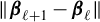 $\|\boldsymbol \beta _{\ell +1} - \boldsymbol \beta _\ell \|$
,
$\|\boldsymbol \beta _{\ell +1} - \boldsymbol \beta _\ell \|$
, $\ell \in \{1, \ldots , R\}$
, asymptotically vanish at an appropriate rate, the weak limits of the change point estimators correspond to the locations of the maxima of two-sided Wiener processes with linear drift, which depend solely on long-run variance parameters that encode the heteroscedasticity of the errors. After estimating this parameter, these results are used to facilitate the construction of confidence intervals for the change points.
$\ell \in \{1, \ldots , R\}$
, asymptotically vanish at an appropriate rate, the weak limits of the change point estimators correspond to the locations of the maxima of two-sided Wiener processes with linear drift, which depend solely on long-run variance parameters that encode the heteroscedasticity of the errors. After estimating this parameter, these results are used to facilitate the construction of confidence intervals for the change points.
In a Monte Carlo simulation study, we evaluated the accuracy of the confidence intervals by analyzing their length and empirical coverage rates. The results show that traditional confidence intervals for the change points can be significantly biased if heteroscedasticity in the model errors is neglected. The proposed confidence intervals constructed under the assumption of potentially heteroscedastic errors exhibit accurate empirical coverage rates in both homoscedastic as well as in heteroscedastic models. Our proposed confidence intervals outperform the methods of Bai and Perron (Reference Bai and Perron2003), Elliott and Müller (Reference Elliott and Müller2007), and Eo and Morley (Reference Eo and Morley2015) in heteroscedastic models. Simulation experiments also verify the usefulness of the information criteria model selection to determine the number of change points, which further ensures the validity of constructing confidence intervals for multiple structural breaks. We then apply the proposed methods to the puzzle of the flattening New Keynesian Phillips curve (Stock and Watson, Reference Stock and Watson2020), examining whether its slope has diminished since the stagflation of the 1970s and identifying several structural breaks in the subsequent decades. Another data application shows that the recently developed cryptocurrency common risk factors (Liu, Tsyvinski, and Wu, Reference Liu, Tsyvinski and Wu2020) fail to explain the excess return of Bitcoin during the burst of the cryptocurrency bubble during the sample period of 2017–2020.
The remainder of the article is structured as follows. Section 2 provides the main results on confidence intervals for the times of changes. Section 3 extends the proposed methods to more generally non-stationary errors. In Section 4, we describe the methods to estimate the times and numbers of changes. Section 5 shows the finite sample performances of the confidence intervals by computing the empirical coverage rates for several simulated data sets. Section 6 presents data applications, and Section 7 concludes. The Supplementary Material provides full technical proofs, algorithms for computing the confidence intervals, additional simulation results, and data examples.
2 MAIN RESULTS ON CONFIDENCE INTERVALS FOR THE TIMES OF CHANGES
We consider the observed data $\{ (\mathbf {x}_1, y_1), \dots , (\mathbf {x}_N, y_N) \}$
, with
$\{ (\mathbf {x}_1, y_1), \dots , (\mathbf {x}_N, y_N) \}$
, with $\mathbf {x}_i \in \mathbb {R}^d$
and
$\mathbf {x}_i \in \mathbb {R}^d$
and $y_i \in \mathbb {R}$
, generated by a linear model with potential change points as defined in (1.1). Throughout the article, we assume that the change points are well spaced in the following sense.
$y_i \in \mathbb {R}$
, generated by a linear model with potential change points as defined in (1.1). Throughout the article, we assume that the change points are well spaced in the following sense.
Assumption 2.1. The change points $k_i = \lfloor N \theta _i \rfloor $
for some break fractions
$k_i = \lfloor N \theta _i \rfloor $
for some break fractions ${0 < \theta _1 < \cdots < \theta _R < 1}$
.
${0 < \theta _1 < \cdots < \theta _R < 1}$
.
We use the notation $\theta _0 = 0$
and
$\theta _0 = 0$
and $\theta _{R+1} = 1$
. To describe the main results, we start with the residuals of the model (1.1),
$\theta _{R+1} = 1$
. To describe the main results, we start with the residuals of the model (1.1),
 $$ \begin{align*}\hat{\epsilon}_i = y_i - \mathbf{x}_i^\top\hat{\boldsymbol \beta}_N, \end{align*} $$
where $\hat {\boldsymbol \beta }_N$
is the least squares estimator based on the entire sample,
$\hat {\boldsymbol \beta }_N$
is the least squares estimator based on the entire sample,
 $$ \begin{align*}\hat{\boldsymbol \beta}_N = \left(\mathbf{X}_N^\top\mathbf{X}_N\right)^\top\mathbf{X}_N^\top\mathbf{Y}_N. \end{align*} $$
Here, $\mathbf {Y}_N = (y_1, \ldots , y_N)^\top $
, and
$\mathbf {Y}_N = (y_1, \ldots , y_N)^\top $
, and
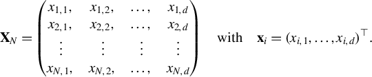 $$ \begin{align*} \mathbf{X}_N = \begin{pmatrix} x_{1,1},\;&x_{1,2},\;&\ldots,\;&x_{1,d}\\ x_{2,1},\;&x_{2,2},\;&\ldots,\;&x_{2,d}\\ \vdots &\vdots &\vdots &\vdots\\ x_{N,1},\;&x_{N,2},\;&\ldots,\;&x_{N,d} \end{pmatrix} \quad\text{with}\quad \mathbf{x}_i = (x_{i,1}, \ldots, x_{i,d})^\top. \end{align*} $$
To test for change points and estimate their number and locations, we use a d-dimensional CUSUM process of the covariate weighted residuals
 $$ \begin{align*}\hat{\mathbf{Z}}_N(k) = \frac{1}{[k(N-k)]^\kappa}\left(\sum_{i=1}^k \mathbf{x}_i \hat{\epsilon}_i - \frac{k}{N} \sum_{i=1}^N \mathbf{x}_i \hat{\epsilon}_i \right), \quad k \in \{1,\dots,N-1\}, \end{align*} $$
where ${[k(N-k)]^{-\kappa }}$
is a weight function with
${[k(N-k)]^{-\kappa }}$
is a weight function with $0 \leq \kappa \leq 1/2$
. Given the definition of
$0 \leq \kappa \leq 1/2$
. Given the definition of $\hat {\boldsymbol \beta }_N$
, the complete sum of the covariate weighted residuals is zero, so that
$\hat {\boldsymbol \beta }_N$
, the complete sum of the covariate weighted residuals is zero, so that
 $$ \begin{align} \hat{\mathbf{Z}}_N(k) = \frac{1}{[k(N-k)]^\kappa} \sum_{i=1}^k \mathbf{x}_i \hat{\epsilon}_i, \quad k \in \{1,\dots,N-1\}. \end{align} $$
We shall assume conditions, which will be detailed in Assumption 2.6, that imply
 $$ \begin{align} \hat{\mathbf{A}}_N = \frac{1}{N} \mathbf{X}_N^\top \mathbf{X}_N \overset{P}{\rightarrow} \mathbf{A} , \end{align} $$
where the matrix $\mathbf {A}$
satisfies the following assumption.
$\mathbf {A}$
satisfies the following assumption.
Assumption 2.2. $ \mathbf {A}$
is a non-singular matrix.
$ \mathbf {A}$
is a non-singular matrix.
We consider asymptotic results for the estimators of $k_1, \dots , k_R$
that presume the existence of preliminary estimators of the change points that are weakly consistent with a mild convergence rate. We show in Section 4 that we can construct such estimators using binary segmentation and model selection based on information criteria. Specifically, we assume we have access to estimators
$k_1, \dots , k_R$
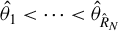
that presume the existence of preliminary estimators of the change points that are weakly consistent with a mild convergence rate. We show in Section 4 that we can construct such estimators using binary segmentation and model selection based on information criteria. Specifically, we assume we have access to estimators $\hat {R}_N$
,
$\hat {R}_N$
, $\hat {\theta }_1 < \cdots < \hat {\theta }_{\hat {R}_N}$
for the parameters
$\hat {\theta }_1 < \cdots < \hat {\theta }_{\hat {R}_N}$
for the parameters $R, \theta _1 < \cdots < \theta _R$
satisfying the following assumption.
$R, \theta _1 < \cdots < \theta _R$
satisfying the following assumption.
Assumption 2.3. For all $\varepsilon>0,$
 $$ \begin{align} \lim_{N\to \infty}P\left( \{|\hat{\theta}_r-\theta_r|\leq \varepsilon\;\;\text{for all}\;\;1\leq r \leq R \} \cap \{ \hat{R}_N=R \} \right)=1. \end{align} $$
Assumption 2.3 requires, as the sample size N increases, that the estimated break fractions $\hat {\theta }_r$
converge in probability to the true parameters
$\hat {\theta }_r$
converge in probability to the true parameters $\theta _r$
. It also states that the estimated number of change points
$\theta _r$
. It also states that the estimated number of change points $\hat {R}_N$
converges in probability to the true number of change points R with probability 1, as N increases. Assumption 2.3 is standard and is satisfied by most standard segmentation algorithms (see, e.g., Fearnhead and Fryzlewicz, Reference Fearnhead and Fryzlewicz2024; Horváth and Rice, Reference Horváth and Rice2024). We define initial change point estimation methods in Section 4 that will satisfy this assumption. In fact, many multiple change point estimation methods will satisfy the much stronger condition in this case that
$\hat {R}_N$
converges in probability to the true number of change points R with probability 1, as N increases. Assumption 2.3 is standard and is satisfied by most standard segmentation algorithms (see, e.g., Fearnhead and Fryzlewicz, Reference Fearnhead and Fryzlewicz2024; Horváth and Rice, Reference Horváth and Rice2024). We define initial change point estimation methods in Section 4 that will satisfy this assumption. In fact, many multiple change point estimation methods will satisfy the much stronger condition in this case that $| \hat {\theta }_r - \theta _r|=O_P(1/N).$
The associated estimates of $k_r$
are
$k_r$
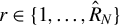
are $\hat {k}_r = \lfloor N \hat {\theta }_r \rfloor $
,
$\hat {k}_r = \lfloor N \hat {\theta }_r \rfloor $
, $r \in \{1,\dots ,\hat {R}_N\}$
. Given such initial estimators, we are interested in deriving simultaneous confidence intervals for the times of changes
$r \in \{1,\dots ,\hat {R}_N\}$
. Given such initial estimators, we are interested in deriving simultaneous confidence intervals for the times of changes $k_\ell $
.
$k_\ell $
.
We consider the heteroscedastic case when the behavior of the $\epsilon _i$
’s might change during the observation period at unknown times. Let the combined process of the covariates and the errors be denoted as
$\epsilon _i$
’s might change during the observation period at unknown times. Let the combined process of the covariates and the errors be denoted as $\mathbf {z}_i = \{ (\mathbf {x}_i, \epsilon _i)^\top , \; i \in \mathbb {Z} \}$
. We allow the process to experience structural changes at M distinct points in time, denoted by
$\mathbf {z}_i = \{ (\mathbf {x}_i, \epsilon _i)^\top , \; i \in \mathbb {Z} \}$
. We allow the process to experience structural changes at M distinct points in time, denoted by $m_1 < \cdots < m_M$
, over the observation period. For each
$m_1 < \cdots < m_M$
, over the observation period. For each $m_\ell $
,
$m_\ell $
, $1 \leq \ell \leq M$
, we assume the following assumption.
$1 \leq \ell \leq M$
, we assume the following assumption.
Assumption 2.4. $m_\ell =\lfloor N\tau _\ell \rfloor $
and
$m_\ell =\lfloor N\tau _\ell \rfloor $
and $0<\tau _1<\cdots <\tau _M<1$
,
$0<\tau _1<\cdots <\tau _M<1$
,
with $m_0 = 0, m_{M+1} = N$
and correspondingly
$m_0 = 0, m_{M+1} = N$
and correspondingly $\tau _0 = 0$
and
$\tau _0 = 0$
and $\tau _{M+1} = 1$
. Davis, Hancock, and Yao (Reference Davis, Hancock and Yao2016), Leybourne et al. (Reference Leybourne, Taylor and Kim2007), Górecki, Horváth, and Kokoszka (Reference Górecki, Horváth and Kokoszka2018), Pein et al. (Reference Pein, Sieling and Munk2017), and Horváth et al. (Reference Horváth, Miller and Rice2021) introduce heteroscedastic models, similar to Assumption 2.4, in change point analysis. Here, we use a decomposable Bernoulli shift model for each segment of stationarity.
$\tau _{M+1} = 1$
. Davis, Hancock, and Yao (Reference Davis, Hancock and Yao2016), Leybourne et al. (Reference Leybourne, Taylor and Kim2007), Górecki, Horváth, and Kokoszka (Reference Górecki, Horváth and Kokoszka2018), Pein et al. (Reference Pein, Sieling and Munk2017), and Horváth et al. (Reference Horváth, Miller and Rice2021) introduce heteroscedastic models, similar to Assumption 2.4, in change point analysis. Here, we use a decomposable Bernoulli shift model for each segment of stationarity.
Assumption 2.5. Assume $\mathbf {z}_i = \mathbf {g}_\ell (\eta _i, \eta _{i-1}, \ldots )$
, for
$\mathbf {z}_i = \mathbf {g}_\ell (\eta _i, \eta _{i-1}, \ldots )$
, for $m_{\ell -1} < i \leq m_{\ell }, \, 1 \leq \ell \leq M\,{+}\,1$
, where
$m_{\ell -1} < i \leq m_{\ell }, \, 1 \leq \ell \leq M\,{+}\,1$
, where $\mathbf {g}_\ell $
are non-random measurable functions,
$\mathbf {g}_\ell $
are non-random measurable functions, ${\mathcal S}^\infty \to \mathbb {R}^{d+1}$
, and
${\mathcal S}^\infty \to \mathbb {R}^{d+1}$
, and $E\|\mathbf {z}_i\|^\nu < \infty $
with some
$E\|\mathbf {z}_i\|^\nu < \infty $
with some $\nu> 4$
. The random variables
$\nu> 4$
. The random variables $\{\eta _i, -\infty < i < \infty \}$
are independent and identically distributed with values in a measurable space
$\{\eta _i, -\infty < i < \infty \}$
are independent and identically distributed with values in a measurable space ${\mathcal S}$
such that
${\mathcal S}$
such that
 $$ \begin{align*}\left( E\left\|\mathbf{z}_i - \mathbf{z}^*_{i,j}\right\|^\nu \right)^{1/\nu} \leq c j^{-\vartheta} \quad \text{with some} \;\; c> 0 \;\; \text{and} \;\; \vartheta > 2, \end{align*} $$
where $\mathbf {z}_{i,j}^* = \mathbf {g}_\ell (\eta _i, \ldots , \eta _{i-j+1}, \eta ^*_{i-j }, \eta _{i-j-1, }^*, \ldots )$
,
$\mathbf {z}_{i,j}^* = \mathbf {g}_\ell (\eta _i, \ldots , \eta _{i-j+1}, \eta ^*_{i-j }, \eta _{i-j-1, }^*, \ldots )$
, $m_{\ell -1} < i \leq m_{\ell }, 1 \leq \ell \leq M+1$
, and
$m_{\ell -1} < i \leq m_{\ell }, 1 \leq \ell \leq M+1$
, and $\{\eta ^*_{\ell },\; \ell \in \mathbb {Z}\}$
are independent, identically distributed copies of
$\{\eta ^*_{\ell },\; \ell \in \mathbb {Z}\}$
are independent, identically distributed copies of $\eta _0$
, independent of
$\eta _0$
, independent of $\{\eta _j, j\in \mathbb {Z}\}$
.
$\{\eta _j, j\in \mathbb {Z}\}$
.
Under Assumption 2.5, the errors are not stationary over the whole observation period, but are approximately stationary on the sub-segments $(m_{\ell -1}, m_\ell ]$
,
$(m_{\ell -1}, m_\ell ]$
, $1 \leq \ell \leq M+1$
. In Section 3, we extend our model to the case where
$1 \leq \ell \leq M+1$
. In Section 3, we extend our model to the case where $\epsilon _i$
is more generally non-stationary on
$\epsilon _i$
is more generally non-stationary on $(m_{\ell -1}, m_\ell ]$
, for
$(m_{\ell -1}, m_\ell ]$
, for $1 \leq \ell \leq M+1$
. When Assumption 2.5 is combined with Assumption 2.2, we are in effect assuming that the model covariates are stationary. We cannot though simplify Assumption 2.5 to only involve the model errors since we require that the covariates and errors remain piecewise jointly stationary. We note also that Assumption 2.5 also allows “dynamic regression” or lagged values of the response, so long as the model admits a stationary and weakly dependent solution (see Chapter 5.2 of Horváth and Rice, Reference Horváth and Rice2024).
$1 \leq \ell \leq M+1$
. When Assumption 2.5 is combined with Assumption 2.2, we are in effect assuming that the model covariates are stationary. We cannot though simplify Assumption 2.5 to only involve the model errors since we require that the covariates and errors remain piecewise jointly stationary. We note also that Assumption 2.5 also allows “dynamic regression” or lagged values of the response, so long as the model admits a stationary and weakly dependent solution (see Chapter 5.2 of Horváth and Rice, Reference Horváth and Rice2024).
Under Assumption 2.5, the long-run covariance matrices,
 $$ \begin{align*}\mathbf{D}_\ell = \lim_{N \to \infty} \frac{1}{m_\ell - m_{\ell-1}} E\left( \sum_{i = m_{\ell-1} + 1}^{m_{\ell}} \mathbf{x}_i \epsilon_i \right) \left( \sum_{i = m_{\ell-1} + 1}^{m_{\ell}} \mathbf{x}_i \epsilon_i \right)^\top, \quad 1 \leq \ell \leq M + 1, \end{align*} $$
are well defined. The identification of the regression parameter requires the following.
Assumption 2.6. $E[\mathbf {x}_{m_\ell } \epsilon _{m_\ell }] = \bf 0$
and
$E[\mathbf {x}_{m_\ell } \epsilon _{m_\ell }] = \bf 0$
and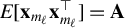 $E[\mathbf {x}_{m_\ell } \mathbf {x}_{m_\ell }^\top ] = \mathbf {A}$
,
$E[\mathbf {x}_{m_\ell } \mathbf {x}_{m_\ell }^\top ] = \mathbf {A}$
, $\ell \in \{1, \dots , M+1\}$
, where
$\ell \in \{1, \dots , M+1\}$
, where $\mathbf {A}$
is the matrix defined in Assumption 2.2.
$\mathbf {A}$
is the matrix defined in Assumption 2.2.
2.1 Exactly One Change Point $(R=1)$

We are now ready to propose our change point estimators and discuss their asymptotic properties. First, let us consider a simple case where only one change point occurs in model (1.1). Given the form of the CUSUM process in (2.1), we use the following estimator to construct confidence intervals:
 $$ \begin{align} \hat{k}_N(\kappa)=\min\left\{k:\;\frac{1}{(k(N-k))^\kappa}\left\|\sum_{i=1}^k\mathbf{x}_i\hat{\epsilon}_i\right\| =\max_{1\leq j <N} \frac{1}{(j(N-j))^\kappa}\left\|\sum_{i=1}^j\mathbf{x}_i\hat{\epsilon}_i\right\| \right\}. \end{align} $$
The weight parameter $\kappa $
can be selected from the interval
$\kappa $
can be selected from the interval $[0, 1/2]$
. For the simulation and empirical sections, we primarily use
$[0, 1/2]$
. For the simulation and empirical sections, we primarily use $\kappa = 1/2$
due to its overall strong performance across various data scenarios. Figure G.7 in the Supplementary Material further discusses and compares the results for
$\kappa = 1/2$
due to its overall strong performance across various data scenarios. Figure G.7 in the Supplementary Material further discusses and compares the results for $\kappa = 0$
,
$\kappa = 0$
, $0.15$
,
$0.15$
, $0.3$
, and
$0.3$
, and $0.45$
.
$0.45$
.
To simplify notation, we use $\theta $
and
$\theta $
and ${k}^*$
in place of
${k}^*$
in place of $\theta _1$
and
$\theta _1$
and $k_1$
for the change point parameters, when
$k_1$
for the change point parameters, when $R = 1$
. We define the size of the change as
$R = 1$
. We define the size of the change as
 $$ \begin{align} \boldsymbol \Delta_N = \boldsymbol \beta_1 - \boldsymbol \beta_2, \end{align} $$
and require the following assumption on its magnitude.
Assumption 2.7. $\|\boldsymbol \Delta _N\|^2 \to 0$
as
$\|\boldsymbol \Delta _N\|^2 \to 0$
as $N \to \infty $
such that (i) if
$N \to \infty $
such that (i) if $0\leq \kappa <1/2$
, then
$0\leq \kappa <1/2$
, then
 $$ \begin{align*}N\|\boldsymbol \Delta_N\|^2\to \infty,\end{align*} $$
(ii) if $\kappa =1/2$
, then
$\kappa =1/2$
, then
 $$ \begin{align*}\frac{N}{\log\log N}\|\boldsymbol \Delta_N\|^2\to \infty. \end{align*} $$
We further define the asymptotic direction of the change as
 $$ \begin{align} \mathbf{d} = \underset{N\rightarrow \infty}{\lim} \frac{\boldsymbol \Delta_N}{\left\| \boldsymbol \Delta_N \right\|}. \end{align} $$
Variance parameters arising in the limiting distribution of $\hat {k}_N$
are
$\hat {k}_N$
are
 $$ \begin{align*} a^2(\theta) = \mathbf{d}^\top \mathbf{A}\mathbf{D}_\ell\mathbf{A} \mathbf{d}, \quad \text{if } \tau_{\ell-1}< \theta <\tau_\ell, \text{ and } a^2(\theta+) = \mathbf{d}^\top \mathbf{A}\mathbf{D}_{\ell+1}\mathbf{A} \mathbf{d}, \quad \text{if } \theta =\tau_{\ell}. \end{align*} $$
Let
 $$ \begin{align} {\sigma}^*=\left(\frac{a(\theta)+a(\theta+)}{2}\right)^2\frac{1 }{\|\mathbf{A} \mathbf{d} \|^4}. \end{align} $$
We define the random variable $\xi (\kappa )$
as
$\xi (\kappa )$
as
 $$ \begin{align} \xi(\kappa)=\xi(\kappa, \theta)=\text{ argmax}_t\left\{ W(t)-|t|m_\kappa(t, \theta) \right\}, \end{align} $$
where
 $$ \begin{align} m_\kappa(t, u)=\left\{ \begin{array}{@{}ll} (1-\kappa)(1-u)+\kappa u,\quad\text{if}\;\;\;t \le 0, \\ (1-\kappa)u+\kappa(1-u), \quad\text{if}\;\;\;t>0, \end{array} \right. \end{align} $$
and
 $$ \begin{align} W(t)=\left\{ \begin{array}{@{}ll} \displaystyle \frac{2a(\theta)}{a(\theta)+a(\theta+)} W_1(-t), \quad\text{if}\;\;\;t<0, \\\displaystyle \frac{2a(\theta+)}{a(\theta)+a(\theta+)} W_2(t), \quad\ \ \ \text{if}\;\;\;t \ge 0, \end{array} \right. \end{align} $$
with $\{W_1(t), t\geq 0\}$
and
$\{W_1(t), t\geq 0\}$
and $\{W_2(t), t\geq 0\}$
being independent standard Wiener processes.
$\{W_2(t), t\geq 0\}$
being independent standard Wiener processes.
Theorem 2.1. If Assumptions 2.1–2.7 hold and $R=1$
, then the estimator (2.4) satisfies
$R=1$
, then the estimator (2.4) satisfies
 $$ \begin{align*}\frac{ \|\boldsymbol \Delta_N\|^2}{\sigma^*} \left(\hat{k}_N-k^*\right)\stackrel{{\mathcal D}}{\to}\xi(\kappa). \end{align*} $$
The distribution of $\xi $
will generally be asymmetric when
$\xi $
will generally be asymmetric when $a(\theta ) \ne a(\theta +)$
. Visualizations of the distribution of
$a(\theta ) \ne a(\theta +)$
. Visualizations of the distribution of $\xi $
are shown in Section G of the Supplementary Material. We note that if
$\xi $
are shown in Section G of the Supplementary Material. We note that if $a(\cdot )$
is continuous at
$a(\cdot )$
is continuous at $\theta $
, so that
$\theta $
, so that $a(\theta ) = a(\theta +)$
, then the process
$a(\theta ) = a(\theta +)$
, then the process $\{W(t), -\infty < t < \infty \}$
is a standard two-sided Wiener process, and this result is consistent with the typical limit distribution of change-point estimators (see, for example, Theorem 2.2.1 of Horváth and Rice, Reference Horváth and Rice2024). Otherwise, in the presence of heteroscedasticity,
$\{W(t), -\infty < t < \infty \}$
is a standard two-sided Wiener process, and this result is consistent with the typical limit distribution of change-point estimators (see, for example, Theorem 2.2.1 of Horváth and Rice, Reference Horváth and Rice2024). Otherwise, in the presence of heteroscedasticity, $a(\cdot )$
is a step function, and the scale parameters of W on either side of the origin reflect how the change in variability affects the distribution of the change point estimator. This introduces asymmetry in the distribution of
$a(\cdot )$
is a step function, and the scale parameters of W on either side of the origin reflect how the change in variability affects the distribution of the change point estimator. This introduces asymmetry in the distribution of $\xi $
. The normalization and scaling terms
$\xi $
. The normalization and scaling terms $a(\theta )$
and
$a(\theta )$
and $a(\theta +)$
in Theorem 2.1 will generally not be known, and must be estimated in practice.
$a(\theta +)$
in Theorem 2.1 will generally not be known, and must be estimated in practice.
2.2 A Confidence Interval for
$k^*$
and Nuisance Parameter Estimation

Theorem 2.1 yields
 $$ \begin{align*}\frac{\|\hat{\boldsymbol \Delta}_N\|^2}{ \hat{\sigma}^*}\left(\hat{k}_N-k^*\right)\stackrel{{\mathcal D}}{\to}\xi(\kappa,\theta), \end{align*} $$
provided that the estimators $\hat {\boldsymbol \Delta }_N$
and
$\hat {\boldsymbol \Delta }_N$
and $\hat {\sigma }^*$
satisfy
$\hat {\sigma }^*$
satisfy $\|\hat {\boldsymbol \Delta }_N\| / \|\boldsymbol \Delta _N\| \to 1$
and
$\|\hat {\boldsymbol \Delta }_N\| / \|\boldsymbol \Delta _N\| \to 1$
and $\hat {\sigma }^* \to \sigma ^*$
in probability. Such estimators may be obtained in the single change point case as follows. We set
$\hat {\sigma }^* \to \sigma ^*$
in probability. Such estimators may be obtained in the single change point case as follows. We set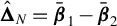 $\hat {\boldsymbol \Delta }_N = \bar {\boldsymbol \beta }_1 - \bar {\boldsymbol \beta }_2$
, with
$\hat {\boldsymbol \Delta }_N = \bar {\boldsymbol \beta }_1 - \bar {\boldsymbol \beta }_2$
, with $\bar {\boldsymbol \beta }_1$
and
$\bar {\boldsymbol \beta }_1$
and $\bar {\boldsymbol \beta }_2$
being the least squares estimates based on observations
$\bar {\boldsymbol \beta }_2$
being the least squares estimates based on observations $(\mathbf {x}_1, y_1), \dots , (\mathbf { x}_{\hat {k}_N(\kappa )}, y_{\hat {k}_N(\kappa )})$
and
$(\mathbf {x}_1, y_1), \dots , (\mathbf { x}_{\hat {k}_N(\kappa )}, y_{\hat {k}_N(\kappa )})$
and $(\mathbf {x}_{\hat {k}_N(\kappa )+1}, y_{\hat {k}_N(\kappa )+1}), \dots , (\mathbf { x}_{N}, y_{N})$
, respectively. We estimate
$(\mathbf {x}_{\hat {k}_N(\kappa )+1}, y_{\hat {k}_N(\kappa )+1}), \dots , (\mathbf { x}_{N}, y_{N})$
, respectively. We estimate $\theta $
with
$\theta $
with $\hat {\theta }=\hat {k}_N/N$
. The qth quantile of the limit distribution
$\hat {\theta }=\hat {k}_N/N$
. The qth quantile of the limit distribution $\xi (\kappa ,\theta )$
, denoted
$\xi (\kappa ,\theta )$
, denoted $\hat {\xi }_q(\kappa ,\hat {\theta })$
, is computed conditionally on the sample. Given a nominal significance level of
$\hat {\xi }_q(\kappa ,\hat {\theta })$
, is computed conditionally on the sample. Given a nominal significance level of $\alpha \in (0,1)$
, these results suggest constructing a
$\alpha \in (0,1)$
, these results suggest constructing a $1 - \alpha $
sized confidence interval for
$1 - \alpha $
sized confidence interval for $k^*$
of the form
$k^*$
of the form
 $$ \begin{align} \left[ \hat{k}_N(\kappa) - \left( \frac{\hat{\xi}_{1-\alpha/2}(\kappa, \hat{\theta}) {\hat{\sigma}}^*}{\|\hat{\boldsymbol \Delta}_N\|^2} \right) , \text{ } \hat{k}_N(\kappa) - \left( \frac{\hat{\xi}_{\alpha/2}(\kappa, \hat{\theta}) {\hat{\sigma}}^*}{\|\hat{\boldsymbol \Delta}_N\|^2} \right) \right]. \end{align} $$
The estimation of $\hat {\sigma }^*$
and
$\hat {\sigma }^*$
and $\hat {\xi }_{q}(\kappa , \hat {\theta })$
further requires the estimation of
$\hat {\xi }_{q}(\kappa , \hat {\theta })$
further requires the estimation of $a(\theta )$
,
$a(\theta )$
, $a(\theta +)$
, and
$a(\theta +)$
, and $\mathbf {A}$
, which we now address. Using the estimators
$\mathbf {A}$
, which we now address. Using the estimators $\bar {\boldsymbol \beta }_1$
and
$\bar {\boldsymbol \beta }_1$
and $\bar {\boldsymbol \beta }_2$
, we define the residuals
$\bar {\boldsymbol \beta }_2$
, we define the residuals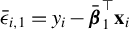 $\bar {\epsilon }_{i,1} = y_i - \bar {\boldsymbol \beta }_1^\top \mathbf {x}_i$
for
$\bar {\epsilon }_{i,1} = y_i - \bar {\boldsymbol \beta }_1^\top \mathbf {x}_i$
for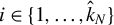 $i \in \{1, \dots , \hat {k}_N\}$
, and
$i \in \{1, \dots , \hat {k}_N\}$
, and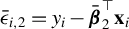 $\bar {\epsilon }_{i,2} = y_i - \bar {\boldsymbol \beta }_2^\top \mathbf {x}_i$
for
$\bar {\epsilon }_{i,2} = y_i - \bar {\boldsymbol \beta }_2^\top \mathbf {x}_i$
for $i \in \{ \hat {k}_N+1, \dots , N\}$
.
$i \in \{ \hat {k}_N+1, \dots , N\}$
.
We show in the proof of Theorem 2.1 that the limit distribution of the normalized $\hat {k}_N$
is determined only by the variables
$\hat {k}_N$
is determined only by the variables $\mathbf { x}_i\hat {\epsilon }_i$
, for
$\mathbf { x}_i\hat {\epsilon }_i$
, for $k^*-\mathcal p _{1,N}\leq i \leq k^*+\mathcal p _{2,N}$
, with any numerical sequences
$k^*-\mathcal p _{1,N}\leq i \leq k^*+\mathcal p _{2,N}$
, with any numerical sequences $\mathcal p _{1,N},\mathcal p _{2,N}$
satisfying
$\mathcal p _{1,N},\mathcal p _{2,N}$
satisfying $\mathcal p _{1,N}\to \infty ,\mathcal p _{2,N}\to \infty $
and
$\mathcal p _{1,N}\to \infty ,\mathcal p _{2,N}\to \infty $
and ${\mathcal p _{1,N}/N\to 0}, \mathcal p _{2,N}/N\to 0$
. We make use of this observation to estimate
${\mathcal p _{1,N}/N\to 0}, \mathcal p _{2,N}/N\to 0$
. We make use of this observation to estimate $a(\theta )$
and
$a(\theta )$
and $a(\theta +)$
. When Assumption 2.4 holds, there is no change in the long run variances of the
$a(\theta +)$
. When Assumption 2.4 holds, there is no change in the long run variances of the $\mathbf {x}_i\hat {\epsilon }_i$
’s when
$\mathbf {x}_i\hat {\epsilon }_i$
’s when $i\in [k^*-\mathcal p _{1,N},\ldots , k^*]$
as well as when
$i\in [k^*-\mathcal p _{1,N},\ldots , k^*]$
as well as when $i\in [k^*+1, \ldots , k^*+\mathcal p _{2,N}]$
. We note that if
$i\in [k^*+1, \ldots , k^*+\mathcal p _{2,N}]$
. We note that if $\theta $
differs from any of the
$\theta $
differs from any of the $\tau _j$
’s, the times of changes of the structure, the long run variance is the same on the whole interval
$\tau _j$
’s, the times of changes of the structure, the long run variance is the same on the whole interval $[k^*-\mathcal p _{1,N},\ldots , k^*+\mathcal p _{2,N}]$
for N sufficiently large. If
$[k^*-\mathcal p _{1,N},\ldots , k^*+\mathcal p _{2,N}]$
for N sufficiently large. If $\theta = \tau _j$
for some
$\theta = \tau _j$
for some $j = 1, \ldots , M$
, i.e., if a variance change in the errors occurs exactly at
$j = 1, \ldots , M$
, i.e., if a variance change in the errors occurs exactly at $k^*$
, then the long run variances differ before and after
$k^*$
, then the long run variances differ before and after $k^*$
. However, it is unknown which case holds for the data. Hence, we define
$k^*$
. However, it is unknown which case holds for the data. Hence, we define
 $$ \begin{align} \hat{\mathbf{D}}_{1,N}=\sum_{\ell=-\infty}^\infty \mathcal{K}\left(\frac{\ell}{h}\right)\hat{\boldsymbol \gamma}_{1,\ell}, \text{ where,} \end{align} $$
 $$ \begin{align} \hat{\boldsymbol \gamma}_{1,\ell}= \left\{ \begin{array}{@{}ll} \displaystyle \frac{1}{\hat{k}_N-\ell}\sum_{j=\hat{k}_N-\mathcal p _{1,N}}^{\hat{k}_N-\ell}\mathbf{x}_j\bar{\epsilon}_{1,j}\mathbf{ x}_{j+\ell}^\top\bar{\epsilon}_{1,j+\ell},\qquad\ \ \;\;\text{if}\;\;\;0\leq \ell<\mathcal p _{1,N}, \\\displaystyle \frac{1}{\hat{k}_N-|\ell|}\sum_{j=\hat{k}_N-\mathcal p _{1,N}-\ell}^{\hat{k}_N}\mathbf{x}_j\bar{\epsilon}_{1,j}\mathbf{ x}_{j+\ell}^\top\bar{\epsilon}_{1,j+\ell},\quad\;\;\text{if}\;\;\;-\mathcal p _{1,N} <\ell<0. \end{array} \right. \end{align} $$
Our estimator for $a(\theta )$
is then
$a(\theta )$
is then
 $$ \begin{align} \hat{a}^2(\theta)=\hat{\mathbf{d}}^\top \hat{\mathbf{A}}_N\hat{\mathbf{D}}_{1,N}\hat{\mathbf{A}}_N\hat{\mathbf{d}}, \end{align} $$
where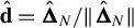 $\hat {\mathbf {d}}=\hat {\boldsymbol \Delta }_N / \|\hat {\boldsymbol \Delta }_N \|$
, and
$\hat {\mathbf {d}}=\hat {\boldsymbol \Delta }_N / \|\hat {\boldsymbol \Delta }_N \|$
, and $\hat {\mathbf {A}}_N$
is defined in (2.2). The definition of the estimator for
$\hat {\mathbf {A}}_N$
is defined in (2.2). The definition of the estimator for $a(\theta +)$
is similar, but based on the variables
$a(\theta +)$
is similar, but based on the variables $\mathbf {x}_i\hat {\epsilon }_i, i\in [\hat {k}_N+1, \ldots ,\hat {k}_N+\mathcal p _{2,N}]$
, so that
$\mathbf {x}_i\hat {\epsilon }_i, i\in [\hat {k}_N+1, \ldots ,\hat {k}_N+\mathcal p _{2,N}]$
, so that
 $$ \begin{align} \hat{a}^2(\theta+)=\hat{\mathbf{d}}^\top\hat{\mathbf{A}}_N\hat{\mathbf{D}}_{2,N}\hat{\mathbf{A}}_N\hat{\mathbf{d}}, \text{ with,} \end{align} $$
 $$ \begin{align} \hat{\mathbf{D}}_{2,N}=\sum_{\ell=-\infty}^\infty \mathcal{K}\left(\frac{\ell}{h}\right)\hat{\boldsymbol \gamma}_{2,\ell}, \text{ and } \end{align} $$
 $$ \begin{align} \hat{\boldsymbol \gamma}_{2,\ell}= \left\{ \begin{array}{@{}ll} \displaystyle \frac{1}{\hat{k}_N-\ell}\sum_{j=\hat{k}_N+1}^{\hat{k}_N+\mathcal p _{2,N}-\ell}\mathbf{x}_j\bar{\epsilon}_{2,j}\mathbf{ x}_{j+\ell}^\top\bar{\epsilon}_{2,j+\ell},\quad\;\;\;\text{if}\;\;\;0\leq \ell<\mathcal p _{2,N}, \\\\[-5pt] \displaystyle \frac{1}{\hat{k}_N-|\ell|}\sum_{j=\hat{k}_N+1-\ell}^{\hat{k}_N+\mathcal p _{2,N}}\mathbf{x}_j\bar{\epsilon}_{2,j}\mathbf{ x}_{j+\ell}^\top\bar{\epsilon}_{2,j+\ell},\quad\;\;\text{if}\;\;\;-\mathcal p _{2,N} <\ell<0. \end{array} \right. \end{align} $$
Throughout the simulations and data applications, we implement such estimators with the Bartlett kernel  , and the bandwidth is selected using the Andrews (Reference Andrews1991) optimal bandwidth procedure, based on the observations from $\{ \hat {k}_N - \mathcal p _{1,N} : \hat {k}_N \}$
for
$\{ \hat {k}_N - \mathcal p _{1,N} : \hat {k}_N \}$
for $\hat {\mathbf {D}}_{1,N}$
and
$\hat {\mathbf {D}}_{1,N}$
and $\{ \hat {k}_N + 1 : \hat {k}_N + \mathcal p _{2,N} \}$
for
$\{ \hat {k}_N + 1 : \hat {k}_N + \mathcal p _{2,N} \}$
for $\hat {\mathbf {D}}_{2,N} $
. The estimators
$\hat {\mathbf {D}}_{2,N} $
. The estimators $\hat {\mathbf {A}}_N$
,
$\hat {\mathbf {A}}_N$
, $\hat {a}(\theta )$
, and
$\hat {a}(\theta )$
, and $\hat {a}(\theta +)$
are then combined to form an estimator
$\hat {a}(\theta +)$
are then combined to form an estimator $\hat {\sigma }^*$
of
$\hat {\sigma }^*$
of $\sigma ^*$
according to the definition in (2.7). The quantile
$\sigma ^*$
according to the definition in (2.7). The quantile $\hat {\xi }_{q}(\kappa , \hat {\theta })$
may be estimated by simulation using the estimated values
$\hat {\xi }_{q}(\kappa , \hat {\theta })$
may be estimated by simulation using the estimated values $\hat {a}(\theta )$
and
$\hat {a}(\theta )$
and $\hat {a}(\theta +)$
.
$\hat {a}(\theta +)$
.
We denote the interval in (2.11), computed in this manner, by $\hat {k}^{HET}_N$
henceforth. Note that the width of the confidence interval, according to (2.11), grows with increasing
$\hat {k}^{HET}_N$
henceforth. Note that the width of the confidence interval, according to (2.11), grows with increasing $\hat {\sigma }^*$
, and shrinks for increasing
$\hat {\sigma }^*$
, and shrinks for increasing $\|\hat {\boldsymbol \Delta }_N\|$
. In addition, both the quantile
$\|\hat {\boldsymbol \Delta }_N\|$
. In addition, both the quantile $\hat {\xi }_{q}$
and
$\hat {\xi }_{q}$
and $\hat {\sigma }^*$
increase with larger estimates of
$\hat {\sigma }^*$
increase with larger estimates of $a(\theta )$
and
$a(\theta )$
and $a(\theta +)$
. As a result, the confidence interval tends to be wider when there is a stronger heteroscedasticity around the change point. Moreover, the confidence interval is typically asymmetric when there is heteroscedasticity near the change point.
$a(\theta +)$
. As a result, the confidence interval tends to be wider when there is a stronger heteroscedasticity around the change point. Moreover, the confidence interval is typically asymmetric when there is heteroscedasticity near the change point.
Under homoscedasticity (M=0), $a(\theta ) = a(\theta +)$
, and we estimate
$a(\theta ) = a(\theta +)$
, and we estimate $a(\theta )$
using a long-run variance estimator based on the entire residual sequence
$a(\theta )$
using a long-run variance estimator based on the entire residual sequence
 $$ \begin{align} \mathbf{x}_i\hat{\epsilon}_{i}^{HO} =\left\{ \begin{array}{@{}ll} \displaystyle \mathbf{x}_i\hat{\epsilon}_{i,1},\;\;\;\text{if}\;\;i \in \{1,... \hat{k}_N\}, \\ \mathbf{x}_i\hat{\epsilon}_{i,2},\;\;\;\text{if}\;\;i \in \{ \hat{k}_N+1,...,N\}. \end{array} \right. \end{align} $$
We label the interval in (2.11) computed in this way with $\hat {k}_N^{HO}$
in later sections.
$\hat {k}_N^{HO}$
in later sections.
The confidence interval $\hat {k}_N^{HET}$
is also valid for homoscedastic data
$\hat {k}_N^{HET}$
is also valid for homoscedastic data $(M=0)$
. Since
$(M=0)$
. Since $\hat {k}_N$
is derived for possibly heteroscedastic data, we expect that it will be wider than
$\hat {k}_N$
is derived for possibly heteroscedastic data, we expect that it will be wider than $\hat {k}_N^{HO}$
in the case of homoscedastic data.
$\hat {k}_N^{HO}$
in the case of homoscedastic data.
2.3 Multiple Change Points (
$R>1$
)

We now consider the case where $R> 1$
. Under Assumption 2.3, we assume the availability of consistent preliminary estimators for the number of change points,
$R> 1$
. Under Assumption 2.3, we assume the availability of consistent preliminary estimators for the number of change points, $\hat {R}_N$
, and their locations,
$\hat {R}_N$
, and their locations, $\hat {k}_i = \lfloor N\hat {\theta }_i \rfloor $
, with
$\hat {k}_i = \lfloor N\hat {\theta }_i \rfloor $
, with $\hat {k}_0 = 1$
and
$\hat {k}_0 = 1$
and $\hat {k}_{\hat {R}_N+1} = N$
. We then estimate
$\hat {k}_{\hat {R}_N+1} = N$
. We then estimate $k_i$
based on the data
$k_i$
based on the data $(y_j, \mathbf {x}_j),\;\; \hat {k}_{i-1}<j\leq \hat {k}_{i+1}$
, by refining the initial estimators via
$(y_j, \mathbf {x}_j),\;\; \hat {k}_{i-1}<j\leq \hat {k}_{i+1}$
, by refining the initial estimators via
 $$ \begin{align} \hat{{\mathfrak k}}_{N,i}=\hat{{\mathfrak k}}_{N,i}(\kappa)=\min&\Bigg\{k\in (\hat{k}_{i-1}, \hat{k}_{i+1}):\;\frac{1}{[(k-\hat{k}_{i-1})(\hat{k}_{i+1}-k)]^\kappa}\Bigg\|\sum_{\ell=\hat{k}_{i-1}+1}^k\mathbf{ x}_\ell\hat{\epsilon}_{i,\ell}\Bigg\|\\ &\hspace{1.5cm}=\max_{\hat{k}_{i-1}< j <\hat{k}_{i+1}} \frac{1}{[(j-\hat{k}_{i-1})(\hat{k}_i-j)]^\kappa}\Bigg\|\sum_{\ell=\hat{k}_{i-1}+1}^j\mathbf{x}_\ell\hat{\epsilon}_{i,\ell}\Bigg\| \Bigg\}\notag \end{align} $$
for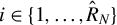 $i \in \{1, \dots , \hat {R}_N\}$
. Let
$i \in \{1, \dots , \hat {R}_N\}$
. Let $\boldsymbol \beta _{i,N}=\hat {\boldsymbol \beta }_{i,N}(\hat {k}_{i-1}, \hat {k}_{i+1})$
be the least square estimator computed from
$\boldsymbol \beta _{i,N}=\hat {\boldsymbol \beta }_{i,N}(\hat {k}_{i-1}, \hat {k}_{i+1})$
be the least square estimator computed from $\{y_\ell $
,
$\{y_\ell $
, $\mathbf {x}_\ell \}$
,
$\mathbf {x}_\ell \}$
,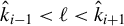 $\hat {k}_{i-1}<\ell <\hat {k}_{i+1}$
. The residuals
$\hat {k}_{i-1}<\ell <\hat {k}_{i+1}$
. The residuals $\hat {\varepsilon }_{i,\ell }$
are obtained from least squares estimation using
$\hat {\varepsilon }_{i,\ell }$
are obtained from least squares estimation using $\{y_\ell , \mathbf {x}_\ell \}$
, i.e.,
$\{y_\ell , \mathbf {x}_\ell \}$
, i.e., $\hat {\varepsilon }_{i,\ell }=y_\ell - \mathbf {x}_\ell ^\top \hat {\boldsymbol \beta }_{i,N}, \hat {k}_{i-1} < \ell < \hat {k}_{i+1} $
.
$\hat {\varepsilon }_{i,\ell }=y_\ell - \mathbf {x}_\ell ^\top \hat {\boldsymbol \beta }_{i,N}, \hat {k}_{i-1} < \ell < \hat {k}_{i+1} $
.
There are two significant theoretical challenges in establishing the joint limiting distribution of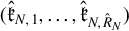 $(\hat {{\mathfrak k}}_{N,1}, \dots , \hat {{\mathfrak k}}_{N,\hat {R}_N})$
. First, although the preliminary estimator for the number of change points
$(\hat {{\mathfrak k}}_{N,1}, \dots , \hat {{\mathfrak k}}_{N,\hat {R}_N})$
. First, although the preliminary estimator for the number of change points $\hat {R}_N$
is assumed to be asymptotically consistent, the dimension of the vector
$\hat {R}_N$
is assumed to be asymptotically consistent, the dimension of the vector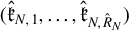 $(\hat {{\mathfrak k}}_{N,1}, \dots , \hat {{\mathfrak k}}_{N,\hat {R}_N})$
for each N is random. Second, even if
$(\hat {{\mathfrak k}}_{N,1}, \dots , \hat {{\mathfrak k}}_{N,\hat {R}_N})$
for each N is random. Second, even if $\hat {R}_N= R$
, the refined change point estimators depend in a complicated way on the preliminary estimates
$\hat {R}_N= R$
, the refined change point estimators depend in a complicated way on the preliminary estimates $\hat {k}_1, \dots , \hat {k}_{\hat {R}_N}$
.
$\hat {k}_1, \dots , \hat {k}_{\hat {R}_N}$
.
In order to address the first challenge, we think of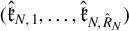 $(\hat {{\mathfrak k}}_{N,1}, \dots , \hat {{\mathfrak k}}_{N,\hat {R}_N})$
as taking value in the disjoint (topological) union of
$(\hat {{\mathfrak k}}_{N,1}, \dots , \hat {{\mathfrak k}}_{N,\hat {R}_N})$
as taking value in the disjoint (topological) union of $\mathbb {R}^k$
,
$\mathbb {R}^k$
,
 $$\begin{align*}\mathbb{U} \;:=\; \bigcup_{k= 0}^\infty \mathbb R^k \; =\; \{(k,\mathbf{x }): k\in\mathbb N \cup \{0\},\; \mathbf{x }\in\mathbb R^k\}. \end{align*}$$ $\mathbb {U}$
is a complete and separable metric space when equipped with the metric
$\mathbb {U}$
is a complete and separable metric space when equipped with the metric

This provides a framework for establishing the weak convergence of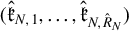 $(\hat {{\mathfrak k}}_{N,1}, \dots , \hat {{\mathfrak k}}_{N,\hat {R}_N})$
, by doing so in the metric space
$(\hat {{\mathfrak k}}_{N,1}, \dots , \hat {{\mathfrak k}}_{N,\hat {R}_N})$
, by doing so in the metric space $\mathbb {U}$
.
$\mathbb {U}$
.
Toward stating the weak limit of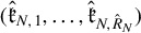 $(\hat {{\mathfrak k}}_{N,1}, \dots , \hat {{\mathfrak k}}_{N,\hat {R}_N})$
, let the size of the parameter change at
$(\hat {{\mathfrak k}}_{N,1}, \dots , \hat {{\mathfrak k}}_{N,\hat {R}_N})$
, let the size of the parameter change at $k_i$
be denoted by
$k_i$
be denoted by $\boldsymbol \Delta _{N,i} = \boldsymbol \beta _i - \boldsymbol \beta _{i+1}$
, and define the variance parameters, with
$\boldsymbol \Delta _{N,i} = \boldsymbol \beta _i - \boldsymbol \beta _{i+1}$
, and define the variance parameters, with $\mathbf {d}_i= \underset {N\rightarrow \infty }{\lim } {\boldsymbol \Delta _{N,i}} /{\| \boldsymbol \Delta _{N,i} \|}$
,
$\mathbf {d}_i= \underset {N\rightarrow \infty }{\lim } {\boldsymbol \Delta _{N,i}} /{\| \boldsymbol \Delta _{N,i} \|}$
,
 $$ \begin{align} \bar{a}(\theta_i)=\mathbf{d}_i^\top\mathbf{A}\mathbf{D}_\ell\mathbf{A}\mathbf{d}_i, \;\tau_{\ell-1}<\theta_i \leq \tau_{\ell}, \text{ and } \bar{a}(\theta_i+)=\left\{ \begin{array}{@{}ll} \mathbf{d}_i^\top\mathbf{A}\mathbf{D}_{\ell}\mathbf{A}\mathbf{d}_i, \;\; \tau_{\ell-1} <\theta_i<\tau_{\ell}, \\ \mathbf{d}_i^\top\mathbf{A}\mathbf{D}_{\ell+1}\mathbf{A}\mathbf{d}_i, \;\; \theta_i=\tau_{\ell}. \end{array} \right. \end{align} $$
Assumption 2.8. $\left \|\boldsymbol \Delta _{N, i}\right \| \rightarrow 0,\text { as }N \rightarrow \infty ,\text { such that } 0<c_1 \leq \left \|\boldsymbol \Delta _{N, i}\right \| /\left \|\boldsymbol \Delta _{N, j}\right \| \leq c_2 \text {, for each } 1 \leq i, j \leq R$
, and (i) if
$\left \|\boldsymbol \Delta _{N, i}\right \| \rightarrow 0,\text { as }N \rightarrow \infty ,\text { such that } 0<c_1 \leq \left \|\boldsymbol \Delta _{N, i}\right \| /\left \|\boldsymbol \Delta _{N, j}\right \| \leq c_2 \text {, for each } 1 \leq i, j \leq R$
, and (i) if $0\leq \kappa <1/2$
, then
$0\leq \kappa <1/2$
, then
 $$ \begin{align*}N^{1/2}\|\boldsymbol \Delta_{N,i}\|\to\infty, \end{align*} $$
(ii) if $\kappa =1/2$
, then
$\kappa =1/2$
, then
 $$ \begin{align*}N^{1/2}(\log N)^{-1/2} \|\boldsymbol \Delta_{N,i}\|\to \infty. \end{align*} $$
Let $W_{1,i}(t), W_{2,i}(t), 0\leq t\leq 1, 1\leq i \leq R$
be independent Wiener processes, and define
$W_{1,i}(t), W_{2,i}(t), 0\leq t\leq 1, 1\leq i \leq R$
be independent Wiener processes, and define
 $$ \begin{align*} W_i(t)=\left\{ \begin{array}{@{}ll} \displaystyle \frac{2\bar{a}(\theta_i)}{\bar{a}(\theta_i)+\bar{a}(\theta_i+)}W_{1,i}(-t), \quad\;\;\text{if}\quad\;\;t<0, \\ \displaystyle \frac{2\bar{a}(\theta_i+)}{\bar{a}(\theta_i)+\bar{a}(\theta_i+)}W_{2,i}(t), \quad\;\;\text{if}\quad\;\;t \geq 0. \end{array} \right. \end{align*} $$
Similarly to $\xi (\kappa , \theta )$
in (2.8), we introduce the independent random variables
$\xi (\kappa , \theta )$
in (2.8), we introduce the independent random variables
 $$ \begin{align*}\xi_i(\kappa, u)= \xi_i(u) = \text{argmax }_t\left\{ W_i(t)-|t|m_\kappa(t, u)\right\}, \end{align*} $$
where $m_\kappa (t,u)$
is defined in (2.9). Let
$m_\kappa (t,u)$
is defined in (2.9). Let
 $$ \begin{align*}\sigma_i^*=\left( \frac{a(\theta_i)+a(\theta_i+)}{2} \right)^2\frac{1}{\|\mathbf{A}\mathbf{d}_i\|^4}. \end{align*} $$
Theorem 2.2. If Assumptions 2.1–2.8 hold, then
 $$ \begin{align*} \left\{ \frac{\|\boldsymbol \Delta_N\|^2}{\sigma^*_i}\left( \hat{\frak{k}}_{N,i}-k_i \right), 1\leq i \leq \hat{R}_N \right\}\stackrel{{\mathcal D}(\mathbb{U})}{\longrightarrow} \left\{ \xi_i\left( \frac{\theta_i-\theta_{i-1}}{\theta_{i+1}-\theta_{i-1}} \right), 1\leq i \leq R \right\}, \end{align*} $$
where $\stackrel {{\mathcal D}(\mathbb {U})}{\longrightarrow }$
denotes weak convergence in
$\stackrel {{\mathcal D}(\mathbb {U})}{\longrightarrow }$
denotes weak convergence in $\mathbb {U}$
.
$\mathbb {U}$
.
Theorem 2.2 can be interpreted as follows: if Assumption 2.3 holds, i.e., the preliminary change point estimators are consistent, then the refined change point estimators $\hat {\mathfrak {k}}_{N, i}$
are consistent, asymptotically independent, and have the distributions as the single change point case described in Theorem 2.1.
$\hat {\mathfrak {k}}_{N, i}$
are consistent, asymptotically independent, and have the distributions as the single change point case described in Theorem 2.1.
2.4 Creating a Confidence Set for
$(k_1,...,k_R)$

Applying Theorem 2.2 to construct a confidence set for $k_1,...,k_R$
requires estimates of the unknown quantities appearing in Theorem 2.2. We proceed along the lines of the discussion in Section 2.2. We define all the terms introduced in Section 2.2 for the subsets of variables
$k_1,...,k_R$
requires estimates of the unknown quantities appearing in Theorem 2.2. We proceed along the lines of the discussion in Section 2.2. We define all the terms introduced in Section 2.2 for the subsets of variables $(\mathbf {x}_{\hat {k}_{i-1}} \hat {\epsilon }_{\hat {k}_{i-1}}, \ldots , \mathbf { x}_{\hat {k}_{i+1}}\hat {\epsilon }_{\hat {k}_{i+1}})$
. Let
$(\mathbf {x}_{\hat {k}_{i-1}} \hat {\epsilon }_{\hat {k}_{i-1}}, \ldots , \mathbf { x}_{\hat {k}_{i+1}}\hat {\epsilon }_{\hat {k}_{i+1}})$
. Let $\hat {\boldsymbol \beta }_{i,1}$
and
$\hat {\boldsymbol \beta }_{i,1}$
and $\hat {\boldsymbol \beta }_{i,2}$
denote the least squares estimates of the regression parameters from the sets
$\hat {\boldsymbol \beta }_{i,2}$
denote the least squares estimates of the regression parameters from the sets $(\mathbf {x}_{\hat {k}_{i-1}}, y_{\hat {k}_{i-1}}), \ldots , (\mathbf { x}_{\hat {k}_i},y_{\hat {k}_i})$
and
$(\mathbf {x}_{\hat {k}_{i-1}}, y_{\hat {k}_{i-1}}), \ldots , (\mathbf { x}_{\hat {k}_i},y_{\hat {k}_i})$
and $(\mathbf {x}_{\hat {k}_i+1},y_{\hat {k}_i+1}). \ldots , (\mathbf {x}_{\hat {k}_{i+1}}, y_{\hat {k}_{i+1}})$
, respectively. The estimator for
$(\mathbf {x}_{\hat {k}_i+1},y_{\hat {k}_i+1}). \ldots , (\mathbf {x}_{\hat {k}_{i+1}}, y_{\hat {k}_{i+1}})$
, respectively. The estimator for $\theta _i$
is
$\theta _i$
is $\hat {\theta }_i=\hat {k}_i/N$
. Let
$\hat {\theta }_i=\hat {k}_i/N$
. Let $\hat {\boldsymbol \Delta }_{N,i}=\hat {\boldsymbol \beta }_{i,1} -\hat {\boldsymbol \beta }_{i,2}$
. By defining numerical sequences
$\hat {\boldsymbol \Delta }_{N,i}=\hat {\boldsymbol \beta }_{i,1} -\hat {\boldsymbol \beta }_{i,2}$
. By defining numerical sequences $\mathcal p _{1,N,i}$
and
$\mathcal p _{1,N,i}$
and $\mathcal p _{2,N,i}$
satisfying
$\mathcal p _{2,N,i}$
satisfying $\mathcal p _{1,N,i}\to \infty , \mathcal p _{2,N,i}\to \infty $
, and
$\mathcal p _{1,N,i}\to \infty , \mathcal p _{2,N,i}\to \infty $
, and $\mathcal p _{1,N,i}/N\to 0, \mathcal p _{2,N,i}/N\to 0$
, we are able to estimate
$\mathcal p _{1,N,i}/N\to 0, \mathcal p _{2,N,i}/N\to 0$
, we are able to estimate $a(\theta _i)$
and
$a(\theta _i)$
and $a(\theta _i+)$
following the procedures (2.12)–(2.14) and (2.15)–(2.17) in Section 2.2.
$a(\theta _i+)$
following the procedures (2.12)–(2.14) and (2.15)–(2.17) in Section 2.2.
The estimator for $\sigma _i^*$
is
$\sigma _i^*$
is
 $$ \begin{align*}\hat{\sigma}_i^*=\left( \frac{\hat{a}(\theta_i)+\hat{a}(\theta_i +)}{2} \right)^2\frac{1}{\|\hat{\mathbf{A}}_N\hat{\mathbf{d}}_{N,i}\|^4}, \text{ with } \hat{\mathbf{d}}_{N,i} = \frac{\hat{\boldsymbol \Delta}_{N,i}}{\|\hat{\boldsymbol \Delta}_{N,i} \|}. \end{align*} $$
Let $\hat {\xi }_q(\kappa , (\hat {\theta }_i-\hat {\theta }_{i-1})/(\hat {\theta }_{i+1}-\hat {\theta }_{i-1}))$
be the qth quantile of
$\hat {\xi }_q(\kappa , (\hat {\theta }_i-\hat {\theta }_{i-1})/(\hat {\theta }_{i+1}-\hat {\theta }_{i-1}))$
be the qth quantile of $\xi _i(\kappa , (\hat {\theta }_i-\hat {\theta }_{i-1})/(\hat {\theta }_{i+1}-\hat {\theta }_{i-1}))$
. For a specified significance level
$\xi _i(\kappa , (\hat {\theta }_i-\hat {\theta }_{i-1})/(\hat {\theta }_{i+1}-\hat {\theta }_{i-1}))$
. For a specified significance level $\alpha>0$
, asymptotic
$\alpha>0$
, asymptotic $1-\alpha $
confidence intervals for the i’th change point are
$1-\alpha $
confidence intervals for the i’th change point are
 $$ \begin{align*} &\hat{I}_i =\Bigg[\hat{{\mathfrak k}}_{N,i}(\kappa) - \hat{\xi}_{1-\alpha/2,i} \left(\kappa, \frac{\hat{\theta}_i-\hat{\theta}_{i-1}}{\hat{\theta}_{i+1}-\hat{\theta}_{i-1}}\right)\frac{\hat{\sigma}_i^*}{\|\hat{\boldsymbol \Delta}_{N,i}\|^2}, \hat{{\mathfrak k}}_{N,i}(\kappa) \\&\quad- \hat{\xi}_{\alpha/2,i} \left(\kappa, \frac{\hat{\theta}_i-\hat{\theta}_{i-1}}{\hat{\theta}_{i+1}-\hat{\theta}_{i-1}}\right)\frac{\hat{\sigma}_i^*}{\|\hat{\boldsymbol \Delta}_{N,i}\|^2}\Bigg], \notag \end{align*} $$
for $1\leq i \leq \hat {R}_N$
. A confidence set for
$1\leq i \leq \hat {R}_N$
. A confidence set for $\{k_1, \dots , k_R\}$
may then be constructed as
$\{k_1, \dots , k_R\}$
may then be constructed as
 $$ \begin{align*}\mathcal{S}_N = \bigcup_{i=1}^{\hat{R}_N} \hat{I}_i. \end{align*} $$
We note that the confidence set $\mathcal {S}_N$
is constructed as a union of intervals rather than a product of intervals since when
$\mathcal {S}_N$
is constructed as a union of intervals rather than a product of intervals since when $\hat {R}_N \ne R$
, we are unable to evaluate whether the vector-valued parameter
$\hat {R}_N \ne R$
, we are unable to evaluate whether the vector-valued parameter $(k_1,...,k_R)$
lies in
$(k_1,...,k_R)$
lies in $\prod _{i=1}^{\hat {R}_N} \hat {I}_i$
. The two formulations are asymptotically equivalent though. An example of a confidence set of the form
$\prod _{i=1}^{\hat {R}_N} \hat {I}_i$
. The two formulations are asymptotically equivalent though. An example of a confidence set of the form $\mathcal {S}_N$
can be seen in Section 6. The following result describes the asymptotic coverage properties of
$\mathcal {S}_N$
can be seen in Section 6. The following result describes the asymptotic coverage properties of $\mathcal {S}_N$
.
$\mathcal {S}_N$
.
Theorem 2.3. If the conditions of Theorem 2.2 are satisfied, then
 $$ \begin{align*}\lim_{N \to \infty} P\left( \{k_1,...,k_R\} \subseteq \mathcal{S}_N \right) = (1- \alpha )^R. \end{align*} $$
The proofs of Theorems 2.1 and 2.3 are given in Section A of the Supplementary Material.
3 SMOOTHLY CHANGING ERROR VARIANCES
So far, we have assumed that the structure of the model errors might abruptly change during the observation period at up to M points, but the errors are otherwise stationary. In this section, we consider the case when there are additionally smooth changes in the variance of the model errors during the intervals $(m_{i-1}, m_i],\; 1 \leq i \leq M+1$
. We hence modify the model in (1.1) to
$(m_{i-1}, m_i],\; 1 \leq i \leq M+1$
. We hence modify the model in (1.1) to

where the errors $\{\epsilon _i, -\infty <i<\infty \}$
are described in Section 2, and
$\{\epsilon _i, -\infty <i<\infty \}$
are described in Section 2, and $g(\cdot )$
satisfies the following assumption.
$g(\cdot )$
satisfies the following assumption.
Assumption 3.1.
g has a finite total variation on $[0,1]$
.
$[0,1]$
.
Model 3.1 allows for both smooth and abrupt changes in the variance of the errors. Let
 $$ \begin{align*}\mathcal {a}(t)=\int_0^tg^2(u)du. \end{align*} $$
We note that the standard deviation of the coordinates of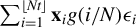 $\sum _{i=1}^{\lfloor Nt\rfloor }\mathbf {x}_i g(i/N)\epsilon _i$
is proportional to
$\sum _{i=1}^{\lfloor Nt\rfloor }\mathbf {x}_i g(i/N)\epsilon _i$
is proportional to $\mathcal {a}(t)$
. We assume the following assumption.
$\mathcal {a}(t)$
. We assume the following assumption.
Assumption 3.2. (i) $0\leq \kappa _1<1/2$
 $$ \begin{align*}\lim_{t\to 0}\frac{1}{t^{ \kappa_1}}\left( \mathcal {a}(t)\log\log(1/ \mathcal {a}(t)) \right)^{1/2}=0, \end{align*} $$
(ii) $0<\kappa _2<1/2$
 $$ \begin{align*}\lim_{t\to 1}\frac{1}{(1-t)^{\kappa_2}}\left( (\mathcal {a}(1)-\mathcal {a}(t))\log\log (1/(\mathcal {a}(1)-\mathcal {a}(t))) \right)^{1/2}=0. \end{align*} $$
We again first consider the case when $R=1$
. We demonstrated in Theorem 2.1 how the limit distribution of the change point estimator is affected by the discontinuity of the variance of the errors. A similar result may be obtained under model (3.1). Let
$R=1$
. We demonstrated in Theorem 2.1 how the limit distribution of the change point estimator is affected by the discontinuity of the variance of the errors. A similar result may be obtained under model (3.1). Let $g(u)$
and
$g(u)$
and $g(u+)$
be the limits of g at u from the left and from the right, respectively. We define
$g(u+)$
be the limits of g at u from the left and from the right, respectively. We define
 $$ \begin{align*} \xi_g(\kappa)=\xi_g(\kappa, \theta)=\text{argmax}_t\left\{ W_g(t)-|t|m_\kappa(t,\theta ) \right\}, \text{ where } \end{align*} $$
 $$ \begin{align*} W_g(t)=\left\{ \begin{array}{@{}ll} \displaystyle \left( \frac{2a(\theta)g(\theta)}{a(\theta)g(\theta)+a(\theta+)g(\theta+)} \right)W_1(-t),\;\;\;\;\;\text{if}\;\;\;t<0, \\\displaystyle \left( \frac{2a(\theta+)g(\theta+)}{a(\theta)g(\theta)+a(\theta+)g(\theta+)} \right)W_2(t),\;\;\;\;\ \ \ \ \text{if}\;\;\;t\geq 0, \end{array} \right. \end{align*} $$
and $\{W_1(s), s\geq 0\}$
and
$\{W_1(s), s\geq 0\}$
and $\{W_2(s), s\geq 0\}$
are independent Wiener processes. Let
$\{W_2(s), s\geq 0\}$
are independent Wiener processes. Let
 $$ \begin{align} \sigma^{*}_g=\left( \frac{a(\theta)g(\theta)+a(\theta+)g(\theta+)}{2} \right)^2\frac{1}{\|\mathbf{A} \mathbf{d}\|^4}. \end{align} $$
Theorem 3.1. If Assumptions 2.1–2.7(i), 3.1, and 3.2 with $\kappa =\min (\kappa _1,\kappa _2)$
hold, then
$\kappa =\min (\kappa _1,\kappa _2)$
hold, then
 $$ \begin{align*} \frac{ \|{\boldsymbol{\Delta}}_N\|^2 } {{\sigma}^{*}_g} \left(\hat{k}_N-k^*\right)\stackrel{{\mathcal D}}{\to}{\xi}_g(\kappa). \end{align*} $$
A confidence interval for $k^*$
based on this result, as in (2.11), can be established in a similar manner.
$k^*$
based on this result, as in (2.11), can be established in a similar manner.
Theorem 3.1 can be adapted in the same manner as Theorem 2.1 to establish an analog of Theorem 2.3 for the multiple change point ( $R> 1$
) case, and the method for constructing a confidence set for the change points detailed in Section 2.3 is valid. We recall the estimators
$R> 1$
) case, and the method for constructing a confidence set for the change points detailed in Section 2.3 is valid. We recall the estimators $\hat {a}^2(\theta )$
and
$\hat {a}^2(\theta )$
and $\hat {a}^2(\theta +)$
defined in (2.14) and (2.15). One can verify that under the conditions of Theorem 3.1,
$\hat {a}^2(\theta +)$
defined in (2.14) and (2.15). One can verify that under the conditions of Theorem 3.1,
 $$ \begin{align} \hat{a}(\theta)\stackrel{P}{\to}a(\theta)g(\theta) \text{ and }\hat{a}(\theta+)\stackrel{P}{\to}a(\theta+)g(\theta+). \end{align} $$
The proof of (3.3) is given in Section D of the Supplementary Material. Hence, the confidence interval in (2.11) is also asymptotically valid under model (3.1). As such, constructing this confidence interval for $k^*$
does not require knowledge of how the second-order properties might change; that is, smooth and/or abrupt changes in the structure and/or variance of the errors do not affect its validity.
$k^*$
does not require knowledge of how the second-order properties might change; that is, smooth and/or abrupt changes in the structure and/or variance of the errors do not affect its validity.
4 TECHNIQUES TO PRELIMINARILY ESTIMATE THE CHANGE POINTS
In this section, we discuss a class of methods to preliminarily estimate the number of changes in model (1.1) such that Assumption 2.3 holds. Many commonly used methods rely on binary segmentation, which begins by splitting the original sample into two sub-samples based on an initial change point estimate, as in (2.4). The procedure is then applied recursively to each sub-sample until the remaining segments are judged to contain no further change points. The determination of the existence of a change point is typically made by checking if a change point test statistic, such as
 $$ \begin{align*}\max_{1\leq j <N} \frac{1}{(j(N-j))^\kappa}\left\|\hat{\mathbf{Z}}_N(k)\right\|, \end{align*} $$
exceeds a threshold parameter $\rho _N$
. Consistency is usually achieved if the parameter
$\rho _N$
. Consistency is usually achieved if the parameter $\rho _N$
satisfies
$\rho _N$
satisfies
 $$ \begin{align} \frac{(\log N)^{1/\nu} }{\rho_N} + \frac{\rho_N}{\sqrt{N}} \to 0, \text{ as } N \to \infty, \end{align} $$
where $\nu $
is the moment parameter defined in Assumption 2.5. It has been shown that, in the case of a simple change in the mean for independent and homoscedastic normal random variables, binary segmentation based on non-weighted CUSUM change point estimators is not consistent. However, the estimators derived from the standardized CUSUM process, with weight function
$\nu $
is the moment parameter defined in Assumption 2.5. It has been shown that, in the case of a simple change in the mean for independent and homoscedastic normal random variables, binary segmentation based on non-weighted CUSUM change point estimators is not consistent. However, the estimators derived from the standardized CUSUM process, with weight function $[t(1-t)]^{1/2}$
, are consistent, so that Assumption 2.3 holds in this case. These results may also be extended to linear models. See Fearnhead and Fryzlewicz (Reference Fearnhead and Fryzlewicz2024) and Horváth and Rice (Reference Horváth and Rice2024).
$[t(1-t)]^{1/2}$
, are consistent, so that Assumption 2.3 holds in this case. These results may also be extended to linear models. See Fearnhead and Fryzlewicz (Reference Fearnhead and Fryzlewicz2024) and Horváth and Rice (Reference Horváth and Rice2024).
Following the proofs of Lemmas A.2 and A.3, one can easily verify that, under the conditions of Theorem 2.3,
 $$ \begin{align*} N^{-1/2+2\kappa}\max_{1\leq k<N}\left\|\hat{\mathbf{Z}}_N(k)-\mathbf{G}_N(k)\right\|=O_P(1), \end{align*} $$
where

It can then be shown, following the arguments of Theorem 2.2 in Rice and Zhang (Reference Rice and Zhang2022), that the binary segmentation method using a threshold satisfying (4.1) and a change-point test statistic defined as the maximum of the weighted CUSUM process with weight parameter $0 < \kappa \leq 1/2$
satisfies Assumption 2.3.
$0 < \kappa \leq 1/2$
satisfies Assumption 2.3.
Another method to estimate the locations and the number of change points is based on model selection criteria. Let K denote a candidate number of possible change points with candidate locations $r_i = \lfloor N \mu _i \rfloor $
,
$r_i = \lfloor N \mu _i \rfloor $
, $0 < \mu _1 < \dots < \mu _K < 1$
(with
$0 < \mu _1 < \dots < \mu _K < 1$
(with $\mu _0 = 0$
,
$\mu _0 = 0$
, $\mu _{K+1} = 1$
). We estimate the change point locations by minimizing the model errors or maximizing the quasi-likelihood ratios over all possible change point locations. This may be framed as an optimization problem of the form
$\mu _{K+1} = 1$
). We estimate the change point locations by minimizing the model errors or maximizing the quasi-likelihood ratios over all possible change point locations. This may be framed as an optimization problem of the form
 $$ \begin{align} \underset{\{ K, \mu_1, \dots, \mu_K \}}{\min } \left ( N\log(\mathscr M(K, \mu_1, \ldots,\mu_K))+ \mathscr P(N,K) \right). \end{align} $$
where $\mathscr M(K, \mu _1, \ldots , \mu _K)$
measures the error of the model, and
$\mathscr M(K, \mu _1, \ldots , \mu _K)$
measures the error of the model, and $\mathscr P(N,K)$
is the penalty term that increases with K. We measure the model error in terms of
$\mathscr P(N,K)$
is the penalty term that increases with K. We measure the model error in terms of
 $$ \begin{align*}\mathscr M(K, \mu_1, \ldots, \mu_K)=\sum_{i=1}^{K+1}\sum_{j=r_{i-1}+1}^{r_i}(y_j- \mathbf{x}_j^\top \hat{\boldsymbol \beta}(r_{i}, r_{i-1}))^2, \end{align*} $$
where $\hat {\boldsymbol \beta }(r_{i}, r_{i-1})$
is the least squares estimator of the regression parameter based on the data with indices between
$\hat {\boldsymbol \beta }(r_{i}, r_{i-1})$
is the least squares estimator of the regression parameter based on the data with indices between $r_{i-1}$
and
$r_{i-1}$
and $r_{i}$
.
$r_{i}$
.
Many typical penalty functions used in the literature can be written in the form $\mathscr P(N,K)=\mathfrak {p}(K)\mathcal m (N)$
, where
$\mathscr P(N,K)=\mathfrak {p}(K)\mathcal m (N)$
, where $\mathfrak {p}(\cdot )$
and
$\mathfrak {p}(\cdot )$
and $\mathcal m (\cdot )$
are strictly increasing functions. These functions can be chosen in several ways. In the case of the Bayesian information criterion (BIC),
$\mathcal m (\cdot )$
are strictly increasing functions. These functions can be chosen in several ways. In the case of the Bayesian information criterion (BIC), $\mathfrak {p}(K)$
is proportional to K and
$\mathfrak {p}(K)$
is proportional to K and $\mathcal m (N) = \log N$
. The BIC criterion is used, for example, in Chakar et al. (Reference Chakar, Lebarbier, Lévy-Leduc and Robin2017) for model selection in AR(1) change point models. In the case of the simplest form of Akaike information criterion (AIC),
$\mathcal m (N) = \log N$
. The BIC criterion is used, for example, in Chakar et al. (Reference Chakar, Lebarbier, Lévy-Leduc and Robin2017) for model selection in AR(1) change point models. In the case of the simplest form of Akaike information criterion (AIC), $\mathfrak {p}(K) = 2K$
and
$\mathfrak {p}(K) = 2K$
and $\mathcal m (N)$
is constant. The choice of
$\mathcal m (N)$
is constant. The choice of $\mathfrak {p}(K) = 2K$
and
$\mathfrak {p}(K) = 2K$
and $\mathcal m (N) = \log \log N$
leads to the Hannan–Quinn information criterion (HQC). We refer to Claeskens and Hjort (Reference Claeskens and Hjort2008) for further reading on model fitting and choices of the penalty term. For both the theoretical and practical aspects of applying model selection methods to change point analysis, we refer the reader to Harchaoui and Lévy-Leduc (Reference Harchaoui and Lévy-Leduc2010), Niu, Hao, and Zhang (Reference Niu, Hao and Zhang2016), Shen, Gallagher, and Lu (Reference Shen, Gallagher and Lu2014), Haynes, Eckley, and Fearnhead (Reference Haynes, Eckley and Fearnhead2017), Wang, Yu, and Rinaldo (Reference Wang, Yu and Rinaldo2020), and Zhang, Li, and Tsai (Reference Zhang, Li and Tsai2010). Many other approaches are discussed in the literature, for instance, using minimum description length as in Davis et al. (Reference Davis, Hancock and Yao2016), or MOSUM (Moving Sum) estimators, see Eichinger and Kirch (Reference Eichinger and Kirch2018) and Kirch and Klein (Reference Kirch and Klein2023), and these have also been shown to satisfy Assumption 2.3.
$\mathcal m (N) = \log \log N$
leads to the Hannan–Quinn information criterion (HQC). We refer to Claeskens and Hjort (Reference Claeskens and Hjort2008) for further reading on model fitting and choices of the penalty term. For both the theoretical and practical aspects of applying model selection methods to change point analysis, we refer the reader to Harchaoui and Lévy-Leduc (Reference Harchaoui and Lévy-Leduc2010), Niu, Hao, and Zhang (Reference Niu, Hao and Zhang2016), Shen, Gallagher, and Lu (Reference Shen, Gallagher and Lu2014), Haynes, Eckley, and Fearnhead (Reference Haynes, Eckley and Fearnhead2017), Wang, Yu, and Rinaldo (Reference Wang, Yu and Rinaldo2020), and Zhang, Li, and Tsai (Reference Zhang, Li and Tsai2010). Many other approaches are discussed in the literature, for instance, using minimum description length as in Davis et al. (Reference Davis, Hancock and Yao2016), or MOSUM (Moving Sum) estimators, see Eichinger and Kirch (Reference Eichinger and Kirch2018) and Kirch and Klein (Reference Kirch and Klein2023), and these have also been shown to satisfy Assumption 2.3.
The optimization in (4.2) is challenging to carry out due to the complexity when the candidate number of change points K is large. In practice, the optimum can be estimated by employing binary segmentation for a decreasing threshold parameter $\rho _N$
, starting from a large
$\rho _N$
, starting from a large $\rho _N$
so that no change points are detected, and then decreasing it to compute candidate change point segmentations, which can be compared on the basis of (4.2). We study this method in the simulations and data analyses below.
$\rho _N$
so that no change points are detected, and then decreasing it to compute candidate change point segmentations, which can be compared on the basis of (4.2). We study this method in the simulations and data analyses below.
5 MONTE CARLO SIMULATION
In this section, we provide a Monte Carlo simulation study to assess the finite sample performance of the estimator $\hat {k}_N$
in (2.4). The first data-generating process (DGP) we consider follows (1.1) with one change point
$\hat {k}_N$
in (2.4). The first data-generating process (DGP) we consider follows (1.1) with one change point $(R=1)$
,
$(R=1)$
,
 $$ \begin{align*} y_i=\left\{ \begin{array}{@{}ll} \mathbf{x}_i^\top\boldsymbol \beta_1+\epsilon_i, \ \quad\quad\qquad \text{if}\;\;\;1<i\leq k_1, \\\mathbf{x}_i^\top(\boldsymbol \beta_1+\boldsymbol \Delta_N)+\epsilon_i, \quad \text{if}\;\;\;k_1< i\leq N, \end{array} \right. \end{align*} $$
where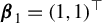 $\boldsymbol \beta _1 = (1, 1)^\top $
, and the covariate
$\boldsymbol \beta _1 = (1, 1)^\top $
, and the covariate $\mathbf {x}_i$
is of the form
$\mathbf {x}_i$
is of the form $\mathbf {x}_i = (x_{1,i}, x_{2,i})^\top $
with
$\mathbf {x}_i = (x_{1,i}, x_{2,i})^\top $
with ${x_1= 1}$
and
${x_1= 1}$
and $x_{2,i}$
independently drawn from a standard normal distribution. We consider different specifications for the error term
$x_{2,i}$
independently drawn from a standard normal distribution. We consider different specifications for the error term $\epsilon _i$
: the first four are stationary, while the latter four allow for heteroscedasticity in various forms. Each time-series process begins after discarding a burn-in sample of length 100, starting from an initial innovation. We consider the following DGPs for the innovations:
$\epsilon _i$
: the first four are stationary, while the latter four allow for heteroscedasticity in various forms. Each time-series process begins after discarding a burn-in sample of length 100, starting from an initial innovation. We consider the following DGPs for the innovations:
-
(i) (IID) The error term,
$\epsilon _i$
, follows an i.i.d. standard normal distribution
$\mathcal {N}(0, 1)$
. -
(ii) (AR) The error term
$\epsilon _i$
is an autoregressive (AR) process of order 1, where the innovations
$$ \begin{align*} \epsilon_i = 0.2\epsilon_{i-1} + \varepsilon_i, \end{align*} $$
$\{ \varepsilon _i \}$
are i.i.d normal random variable
$\mathcal {N}(0, 1)$
.
-
(iii) (AR-HP) The error term
$\epsilon _i$
is a highly-persistent AR(1) process, where the innovations
$$ \begin{align*} \epsilon_i = 0.7\epsilon_{i-1} + \varepsilon_i, \end{align*} $$
$\{ \varepsilon _i \}$
are again standard normal.
-
(iv) (GARCH) The error term
$\epsilon _i$
follows a stationary GARCH(1,1) process where the innovations
$$ \begin{align*} \epsilon_i = h_i^{1/2} \varepsilon_i, \text{ with } h_i = 0.05 + 0.03 \epsilon_{i-1}^2 + 0.85 h_{i-1}, \end{align*} $$
$\{ \varepsilon _i \}$
are i.i.d standard normal.
-
(v) (HeteIID) The error term is a heteroscedastic i.i.d. process that
$$ \begin{align*} \epsilon_i = \left\{\begin{matrix} \epsilon_i \sim \mathcal{N}(0 , 3 ) & 1\leq i\leq m_1,\\ \epsilon_i \sim \mathcal{N}(0 , 0.5) & m_1< i \leq N. \end{matrix}\right. \end{align*} $$
The variance of the error changes at time
$m_1$
, which may or may not coincide with
$k_1$
. -
(vi) (HeteAR) The error follows a heteroscedastic AR process,
where the innovations
$$ \begin{align*} \epsilon_i = \left\{\begin{matrix} 0.2\epsilon_{i-1} + \varepsilon_{1,i} & 1\leq i\leq m_1,\\ 0.2\epsilon_{i-1} + \varepsilon_{2,i} & m_1< i \leq N, \end{matrix}\right. \end{align*} $$
$\{\varepsilon _{1,i}, \varepsilon _{2,i} \}$
are normal distributed process with mean zero and standard deviations
$3$
and
$0.5$
, respectively. The DGP is denoted as HeteAR-HP when the AR coefficient is set to 0.7.
-
(vii) (HeteGARCH) The error term follows a heteroscedastic GARCH process,
where the innovations
$$ \begin{align*} \epsilon_i = h_i^{1/2} \varepsilon_i, \quad h_i = \left\{\begin{matrix} 3 + 0.03 \epsilon_{i-1}^2 + 0.85 h_{i-1}, & 1\leq i\leq m_1\\ 0.5 + 0.03 \epsilon_{i-1}^2 + 0.85 h_{i-1}, & m_1< i \leq N, \end{matrix}\right. \end{align*} $$
$\{ \varepsilon _i \}$
are i.i.d standard normal random variables.
-
(viii) (HeteSmooth) Lastly, the error term follows a heteroscedastic smooth variance change process,
$$ \begin{align*} \epsilon_i = g\left(\frac{i}{N} \right) \varepsilon_i, \text{ for } g\left(\frac{i}{N} \right) = 1+\frac{2}{1+ \exp(-10 (i/N - 0.5) )}. \end{align*} $$





We set the size of change as
 $$ \begin{align*}\boldsymbol \Delta_N=c_1N^{-1/5}(1,1)^\top \zeta_{SNR},\end{align*} $$
with $c_1 \in \{ 1, 3\}$
. We set
$c_1 \in \{ 1, 3\}$
. We set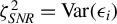 $\zeta _{SNR}^2 = \text {Var}(\epsilon _i)$
for the homoscedastic DGPs,
$\zeta _{SNR}^2 = \text {Var}(\epsilon _i)$
for the homoscedastic DGPs, $\zeta _{SNR}^2 = \theta a^2(\theta ) + (1-\theta ) a^2(\theta +)$
for the heteroscedastic DGPs, and
$\zeta _{SNR}^2 = \theta a^2(\theta ) + (1-\theta ) a^2(\theta +)$
for the heteroscedastic DGPs, and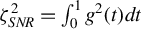 $\zeta _{SNR}^2= \int _0^1 g^2(t)dt$
for the smoothly changing variance DGP in order to make the signal-to-noise ratio comparable across all DGPs. The change point location
$\zeta _{SNR}^2= \int _0^1 g^2(t)dt$
for the smoothly changing variance DGP in order to make the signal-to-noise ratio comparable across all DGPs. The change point location $k_1$
is set to either
$k_1$
is set to either $\lfloor 0.2 N \rfloor $
or
$\lfloor 0.2 N \rfloor $
or $\lfloor 0.5 N \rfloor $
.Footnote
1
We consider two scenarios subsequently for
$\lfloor 0.5 N \rfloor $
.Footnote
1
We consider two scenarios subsequently for $m_1$
: either
$m_1$
: either $m_1 = k_1$
(coinciding with the change point) or
$m_1 = k_1$
(coinciding with the change point) or $m_1 \neq k_1$
(e.g.,
$m_1 \neq k_1$
(e.g., $m_1 = \lfloor 0.5 N \rfloor $
when
$m_1 = \lfloor 0.5 N \rfloor $
when ${k_1 = \lfloor 0.2 N \rfloor }$
). We consider sample sizes of
${k_1 = \lfloor 0.2 N \rfloor }$
). We consider sample sizes of $N \in \{100, 300\}$
.
$N \in \{100, 300\}$
.
5.1 Comparisons of Confidence Interval Coverage and Size
We examine the confidence interval estimators introduced in Sections 2 and 3, assuming either homoscedasticity or heteroscedasticity, respectively labeled $\hat {k}^{HO}_N(\kappa )$
or
$\hat {k}^{HO}_N(\kappa )$
or $\hat {k}^{HET}_N(\kappa )$
(with
$\hat {k}^{HET}_N(\kappa )$
(with $\mathcal p _{1,N} = \mathcal p _{2,N} = \lfloor N^{1/2} \rfloor $
). In order to estimate the quantiles
$\mathcal p _{1,N} = \mathcal p _{2,N} = \lfloor N^{1/2} \rfloor $
). In order to estimate the quantiles $\xi _{q}(\kappa , \hat {\theta })$
and
$\xi _{q}(\kappa , \hat {\theta })$
and $\xi _{g,q}(\kappa , \hat {\theta })$
, we use the corresponding empirical quantile generated from 5,000 replications of two-sided Wiener processes using a sample size of
$\xi _{g,q}(\kappa , \hat {\theta })$
, we use the corresponding empirical quantile generated from 5,000 replications of two-sided Wiener processes using a sample size of $20{,}000$
. The tuning parameter
$20{,}000$
. The tuning parameter $\kappa \in [0, 0.5]$
is typically used in weighted CUSUM-type statistics for change point detection and estimation. When
$\kappa \in [0, 0.5]$
is typically used in weighted CUSUM-type statistics for change point detection and estimation. When $\kappa $
is chosen from the interval
$\kappa $
is chosen from the interval $[0, 1/2)$
, smaller values of
$[0, 1/2)$
, smaller values of $\kappa $
tend to yield higher coverage rates for change points occurring in the middle of the sample, while larger values improve coverage for changes near the boundaries. Setting
$\kappa $
tend to yield higher coverage rates for change points occurring in the middle of the sample, while larger values improve coverage for changes near the boundaries. Setting $\kappa = 1/2$
generally provides more uniform coverage across the entire sample, and this choice is used in the simulations and data applications.
$\kappa = 1/2$
generally provides more uniform coverage across the entire sample, and this choice is used in the simulations and data applications.
We compare our method to three other methods that have been studied under heteroscedastic DGPs in Chang and Perron (Reference Chang and Perron2018), although these methods were not designed for heteroscedastic errors. These include the sum of squared residuals-based estimators–BP (Bai, Reference Bai1997a, Reference Bai1997b; Bai and Perron, Reference Bai and Perron2003), the local powerful estimators–EM (Elliott and Müller, Reference Elliott and Müller2007), and the likelihood ratio statistics-based estimators–ILR (Eo and Morley, Reference Eo and Morley2015). In total, six confidence interval candidates are assessed in the simulation. To evaluate confidence intervals, we compute the empirical coverage rates and the lengths of the confidence intervals calibrated to the 95% level from 2,000 simulations. The empirical coverage rate measures the frequency with which the true change location falls into the empirical confidence intervals. The length of the confidence intervals is normalized with respect to the sample size so that it falls in $(0, 1)$
.
$(0, 1)$
.
Figure 1 shows the empirical coverage rates and the average lengths of the confidence intervals when the models are generated with homoscedastic errors and the change point occurs early in the sample, i.e., $k_1= \lfloor 0.2N \rfloor $
. The sample size
$k_1= \lfloor 0.2N \rfloor $
. The sample size $N=300$
, roughly covers practical cases of more than one year of daily equity return data or 25 years of monthly economic data. The results indicate that all six estimators generally produce reasonably good empirical coverage rates in models with homoscedastic IID, AR, and GARCH errors when the size of the change is large. The lengths of the confidence intervals also narrow as the size of the change increases in magnitude. The
$N=300$
, roughly covers practical cases of more than one year of daily equity return data or 25 years of monthly economic data. The results indicate that all six estimators generally produce reasonably good empirical coverage rates in models with homoscedastic IID, AR, and GARCH errors when the size of the change is large. The lengths of the confidence intervals also narrow as the size of the change increases in magnitude. The $EM$
approach demonstrates high empirical coverage rates in models with small changes. However, this approach results in the longest confidence intervals, which are typically between 3 and 5 times longer than the intervals
$EM$
approach demonstrates high empirical coverage rates in models with small changes. However, this approach results in the longest confidence intervals, which are typically between 3 and 5 times longer than the intervals $\hat {k}^{HET}_N(1/2)$
. This finding is consistent with the simulation results reported by Chang and Perron (Reference Chang and Perron2018). The same general patterns are observed when the error term follows the homoscedastic DGP AR-HP, although the empirical coverage rates are lower.
$\hat {k}^{HET}_N(1/2)$
. This finding is consistent with the simulation results reported by Chang and Perron (Reference Chang and Perron2018). The same general patterns are observed when the error term follows the homoscedastic DGP AR-HP, although the empirical coverage rates are lower.
Empirical coverage rates of BP, EM, ILR, $\hat {k}^{HO}_N(1/2),$
and
$\hat {k}^{HO}_N(1/2),$
and $\hat {k}^{HET}_N(1/2)$
. The DGPs include models with homoscedastic IID, AR, AR-HP, and GARCH errors. For each estimator, the left-side blue bars and right-side red bars present the results when the size of change
$\hat {k}^{HET}_N(1/2)$
. The DGPs include models with homoscedastic IID, AR, AR-HP, and GARCH errors. For each estimator, the left-side blue bars and right-side red bars present the results when the size of change $\Delta _{N,1}=N^{-1/5}(1,1)^\top \zeta _{SNR}$
and
$\Delta _{N,1}=N^{-1/5}(1,1)^\top \zeta _{SNR}$
and $\Delta _{N,2}=3N^{-1/5}(1,1)^\top \zeta _{SNR}$
, respectively. The values displayed on the top of the bar charts document the lengths of confidence intervals, in proportion to the sample size. The change point occurs at the middle of the sample
$\Delta _{N,2}=3N^{-1/5}(1,1)^\top \zeta _{SNR}$
, respectively. The values displayed on the top of the bar charts document the lengths of confidence intervals, in proportion to the sample size. The change point occurs at the middle of the sample $k_1= \lfloor 0.2N \rfloor $
, with the sample size
$k_1= \lfloor 0.2N \rfloor $
, with the sample size $N=300$
.
$N=300$
.
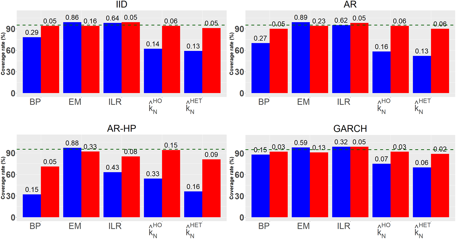
We then turn to the results for heteroscedastic models, reported in Figure 2. The subplots in the left column display results for heteroscedastic errors when the variance change $m_1 = 0.2$
coincides with the change point
$m_1 = 0.2$
coincides with the change point $k_1 = 0.2$
, while the subplots in the right column show results when the variance change
$k_1 = 0.2$
, while the subplots in the right column show results when the variance change $m_1 = 0.5$
differs from
$m_1 = 0.5$
differs from $k_1 = 0.2$
. The remarkable findings can be summarized as follows. First, the BP, EM, and
$k_1 = 0.2$
. The remarkable findings can be summarized as follows. First, the BP, EM, and $\hat {k}^{HO}_N(1/2)$
estimators exhibit deteriorated performance in terms of empirical coverage rates and confidence interval lengths. These estimators do not account for heteroscedasticity by design. As in the homoscedastic case, EM achieves higher coverage rates, but at the cost of excessively long confidence intervals. Second, the
$\hat {k}^{HO}_N(1/2)$
estimators exhibit deteriorated performance in terms of empirical coverage rates and confidence interval lengths. These estimators do not account for heteroscedasticity by design. As in the homoscedastic case, EM achieves higher coverage rates, but at the cost of excessively long confidence intervals. Second, the $ILR$
estimator performs competitively when the variance change
$ILR$
estimator performs competitively when the variance change $m_1$
coincides with the change point
$m_1$
coincides with the change point $k_1$
, but its performance deteriorates substantially in the more general case where
$k_1$
, but its performance deteriorates substantially in the more general case where $m_1 \neq k_1$
. This is expected, since the
$m_1 \neq k_1$
. This is expected, since the $ILR$
estimator assumes simultaneous changes in both variance and coefficients, but it fails with wider confidence intervals and lower coverage when the variance change differs from the coefficient change. Third, we find a considerable correction in the empirical coverage rates when using the intervals
$ILR$
estimator assumes simultaneous changes in both variance and coefficients, but it fails with wider confidence intervals and lower coverage when the variance change differs from the coefficient change. Third, we find a considerable correction in the empirical coverage rates when using the intervals $\hat {k}^{HET}_N(1/2)$
. These confidence intervals achieve coverage close to the nominal level for heteroscedastic DGPs with moderate-sized changes, regardless of whether
$\hat {k}^{HET}_N(1/2)$
. These confidence intervals achieve coverage close to the nominal level for heteroscedastic DGPs with moderate-sized changes, regardless of whether $m_1=k_1$
or
$m_1=k_1$
or $m_1\neq k_1$
. Section G of the Supplementary Material reports additional simulation results. Specifically, we consider
$m_1\neq k_1$
. Section G of the Supplementary Material reports additional simulation results. Specifically, we consider $k_1= \lfloor 0.5N \rfloor $
with
$k_1= \lfloor 0.5N \rfloor $
with $m_1= \lfloor 0.2N \rfloor $
or
$m_1= \lfloor 0.2N \rfloor $
or $\lfloor 0.5N \rfloor $
when
$\lfloor 0.5N \rfloor $
when $N=300$
(Figures G.2 and G.3 in the Supplementary Material), and
$N=300$
(Figures G.2 and G.3 in the Supplementary Material), and $k_1= \lfloor 0.2N \rfloor $
with
$k_1= \lfloor 0.2N \rfloor $
with $m_1= \lfloor 0.2N \rfloor $
or
$m_1= \lfloor 0.2N \rfloor $
or $\lfloor 0.5N \rfloor $
when
$\lfloor 0.5N \rfloor $
when $N=100$
(Figures G.4 and G.5 in the Supplementary Material). We also examine alternative choices of
$N=100$
(Figures G.4 and G.5 in the Supplementary Material). We also examine alternative choices of $\mathcal p _{1,N}$
,
$\mathcal p _{1,N}$
, $\mathcal p _{2,N}$
for
$\mathcal p _{2,N}$
for $\hat {k}^{HET}_N(\kappa )$
(Figure G.6 in the Supplementary Material), different values of
$\hat {k}^{HET}_N(\kappa )$
(Figure G.6 in the Supplementary Material), different values of $\kappa \in \{0, 0.15, 0.3, 0.45\}$
(Figure G.7 in the Supplementary Material), and various signal-to-noise ratios (Figure G.8 in the Supplementary Material).
$\kappa \in \{0, 0.15, 0.3, 0.45\}$
(Figure G.7 in the Supplementary Material), and various signal-to-noise ratios (Figure G.8 in the Supplementary Material).
Empirical coverage rates of BP, EM, ILR, $\hat {k}^{HO}_N(1/2),$
and
$\hat {k}^{HO}_N(1/2),$
and $\hat {k}^{HET}_N(1/2)$
. The DGPs include models with homoscedastic IID, AR, AR-HP, and GARCH, and heteroscedastic HeteIID, HeteAR(-HP), HeteGARCH, and HeteSmooth errors. For each estimator, the left-side blue bars and right-side red bars present the results when the size of change
$\hat {k}^{HET}_N(1/2)$
. The DGPs include models with homoscedastic IID, AR, AR-HP, and GARCH, and heteroscedastic HeteIID, HeteAR(-HP), HeteGARCH, and HeteSmooth errors. For each estimator, the left-side blue bars and right-side red bars present the results when the size of change $\Delta _{N,1}= N^{-1/5}(1,1)^\top \zeta _{SNR}$
and
$\Delta _{N,1}= N^{-1/5}(1,1)^\top \zeta _{SNR}$
and $\Delta _{N,2}=3N^{-1/5}(1,1)^\top \zeta _{SNR}$
, respectively. The values displayed on the top of the bar charts document the average length of confidence intervals, in proportion to the sample size. The change point is set at the beginning of the sample,
$\Delta _{N,2}=3N^{-1/5}(1,1)^\top \zeta _{SNR}$
, respectively. The values displayed on the top of the bar charts document the average length of confidence intervals, in proportion to the sample size. The change point is set at the beginning of the sample, $k_1 = \lfloor 0.2N \rfloor $
, with the error variance change either coinciding at
$k_1 = \lfloor 0.2N \rfloor $
, with the error variance change either coinciding at $m_1 = \lfloor 0.2N \rfloor $
or differing at
$m_1 = \lfloor 0.2N \rfloor $
or differing at $m_1 = \lfloor 0.5N \rfloor $
, under a sample size of
$m_1 = \lfloor 0.5N \rfloor $
, under a sample size of $N = 300$
.
$N = 300$
.
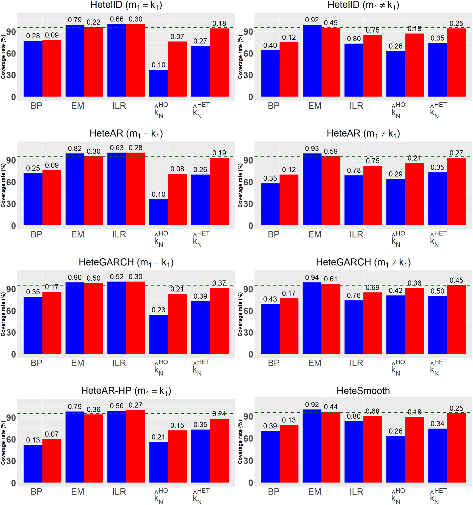
5.2 Multiple Change Point Estimators under Heteroscedasticity
We also consider multiple change point models and assess the methods for preliminarily determining the change point locations as discussed in Section 4. We employ binary segmentation with a decreasing threshold $\rho _N$
in an attempt to minimize the BIC information criterion with a penalty term
$\rho _N$
in an attempt to minimize the BIC information criterion with a penalty term $\mathscr P=2K \times \log (N)/N$
. We decrease
$\mathscr P=2K \times \log (N)/N$
. We decrease $\rho _N$
until a maximum of 7 change points are estimated, and select the model that minimizes the criterion in (4.2). Each simulation was repeated 2,000 times.
$\rho _N$
until a maximum of 7 change points are estimated, and select the model that minimizes the criterion in (4.2). Each simulation was repeated 2,000 times.
In the following experiments, we specifically narrow the DGPs and focus on three types: IID, AR, and HeteAR. Multiple change points ( $R=2,3$
) are introduced in model (1.1) by setting
$R=2,3$
) are introduced in model (1.1) by setting $k_1 = \lfloor 0.2N \rfloor $
,
$k_1 = \lfloor 0.2N \rfloor $
, $k_2 = \lfloor 0.5N \rfloor $
for
$k_2 = \lfloor 0.5N \rfloor $
for $R=2$
, and additionally
$R=2$
, and additionally $k_3 = \lfloor 0.8N \rfloor $
for
$k_3 = \lfloor 0.8N \rfloor $
for $R=3$
, with equal change magnitudes given by either
$R=3$
, with equal change magnitudes given by either $\boldsymbol \Delta _{N,1} = N^{-1/5}(1,1)^\top $
or
$\boldsymbol \Delta _{N,1} = N^{-1/5}(1,1)^\top $
or $\boldsymbol \Delta _{N,2} = 3N^{-1/5}(1,1)^\top $
. In particular, for heteroscedastic HeteAR errors, the variance change locations
$\boldsymbol \Delta _{N,2} = 3N^{-1/5}(1,1)^\top $
. In particular, for heteroscedastic HeteAR errors, the variance change locations $m_1$
,
$m_1$
, $m_2$
, and
$m_2$
, and $m_3$
are set to coincide with
$m_3$
are set to coincide with $k_1$
,
$k_1$
, $k_2$
, and
$k_2$
, and $k_3$
, for simplicity. The independent normal innovations
$k_3$
, for simplicity. The independent normal innovations $\{\varepsilon _{1,i} \sim \mathcal {N}(0,3), \varepsilon _{2,i} \sim \mathcal {N}(0,0.5)\}$
are alternated across segments.
$\{\varepsilon _{1,i} \sim \mathcal {N}(0,3), \varepsilon _{2,i} \sim \mathcal {N}(0,0.5)\}$
are alternated across segments.
Table 1 reports the percentage of models selected as optimal by the BIC criterion when the true number of change points is $R=\{2, 3\}$
. When estimated with either homoscedastic or heteroscedastic errors, the BIC most often selects the correct model when the size of the change is moderate (
$R=\{2, 3\}$
. When estimated with either homoscedastic or heteroscedastic errors, the BIC most often selects the correct model when the size of the change is moderate ( $\boldsymbol \Delta _{N,2}$
). Under HeteAR, the BIC criterion tends to relatively overestimate the number of changes. In contrast, the number of change points is frequently underestimated when the size of the change is small (
$\boldsymbol \Delta _{N,2}$
). Under HeteAR, the BIC criterion tends to relatively overestimate the number of changes. In contrast, the number of change points is frequently underestimated when the size of the change is small ( $\boldsymbol \Delta _{N,1}$
). These results suggest that when the size of the change is small enough, the model selection method tends to ignore such changes in an effort to avoid overfitting.
$\boldsymbol \Delta _{N,1}$
). These results suggest that when the size of the change is small enough, the model selection method tends to ignore such changes in an effort to avoid overfitting.
The frequency from 2,000 simulations at which $\hat {R}_N$
computed via BIC and binary segmentation takes values in
$\hat {R}_N$
computed via BIC and binary segmentation takes values in $\{0,1,2,3\}$
or was larger than or equal to 4.
$\{0,1,2,3\}$
or was larger than or equal to 4.
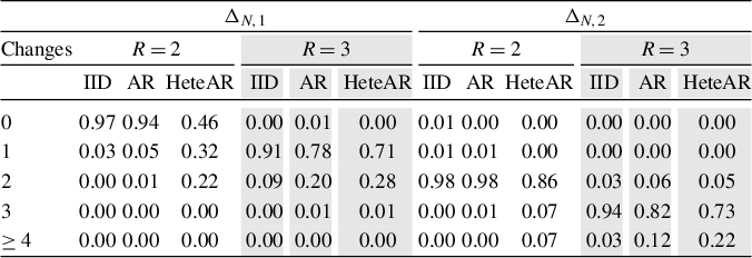
Note: The DGPs include models with IID, AR, and HeteAR errors. The change in the regression parameters was either $\boldsymbol \Delta _{N,1}=N^{-1/5}(1,1)^\top \zeta _{SNR}$
or
$\boldsymbol \Delta _{N,1}=N^{-1/5}(1,1)^\top \zeta _{SNR}$
or $\boldsymbol \Delta _{N,2}=3N^{-1/5}(1,1)^\top \zeta _{SNR}$
, and the sample size
$\boldsymbol \Delta _{N,2}=3N^{-1/5}(1,1)^\top \zeta _{SNR}$
, and the sample size $N=300$
.
$N=300$
.
We now assess how model selection bias affects the empirical coverage rates of confidence intervals for multiple change points. The analysis focuses on DGPs with $R=3$
and moderate change magnitude
$R=3$
and moderate change magnitude $\boldsymbol \Delta _{N,2}$
, excluding small changes since Table 1 shows they lead to underestimation of the number of changes and thus lower coverage. Figure 3 shows that, in homoscedastic models, the empirical coverage rates of all three estimators approach the nominal level of
$\boldsymbol \Delta _{N,2}$
, excluding small changes since Table 1 shows they lead to underestimation of the number of changes and thus lower coverage. Figure 3 shows that, in homoscedastic models, the empirical coverage rates of all three estimators approach the nominal level of $0.95^3 = 0.857$
, as predicted by Theorem 2.2. The empirical coverage rates are slightly undersized, as coverage fails when the number of change points is underestimated, with a 3%–6% probability as shown in Table 1. This underestimation diminishes as the magnitude of change increases. In heteroscedastic models, the empirical coverage rates reach the nominal level for
$0.95^3 = 0.857$
, as predicted by Theorem 2.2. The empirical coverage rates are slightly undersized, as coverage fails when the number of change points is underestimated, with a 3%–6% probability as shown in Table 1. This underestimation diminishes as the magnitude of change increases. In heteroscedastic models, the empirical coverage rates reach the nominal level for $\hat {k}_N^{HET}$
.
$\hat {k}_N^{HET}$
.
Empirical coverage rates of $\hat {k}^{HO}_N(1/2)$
and
$\hat {k}^{HO}_N(1/2)$
and $\hat {k}^{HET}_N(1/2)$
. The DGPs include models with homoscedastic IID, AR, and heteroscedastic HeteAR errors. The teal dotted line represents the nominal level of 85.7% (
$\hat {k}^{HET}_N(1/2)$
. The DGPs include models with homoscedastic IID, AR, and heteroscedastic HeteAR errors. The teal dotted line represents the nominal level of 85.7% ( $0.95^3$
), and the size of change
$0.95^3$
), and the size of change $\boldsymbol \Delta _{N,2}=3N^{-1/5}(1,1)^\top \zeta _{SNR}$
. The values displayed on the top of the bar charts document the average length of confidence intervals, in proportion to the sample size. The change point occurs at
$\boldsymbol \Delta _{N,2}=3N^{-1/5}(1,1)^\top \zeta _{SNR}$
. The values displayed on the top of the bar charts document the average length of confidence intervals, in proportion to the sample size. The change point occurs at $k^*= [\lfloor 0.2N \rfloor , \lfloor 0.5N \rfloor , \lfloor 0.8N \rfloor ] $
, with the sample size
$k^*= [\lfloor 0.2N \rfloor , \lfloor 0.5N \rfloor , \lfloor 0.8N \rfloor ] $
, with the sample size $N=300$
.
$N=300$
.
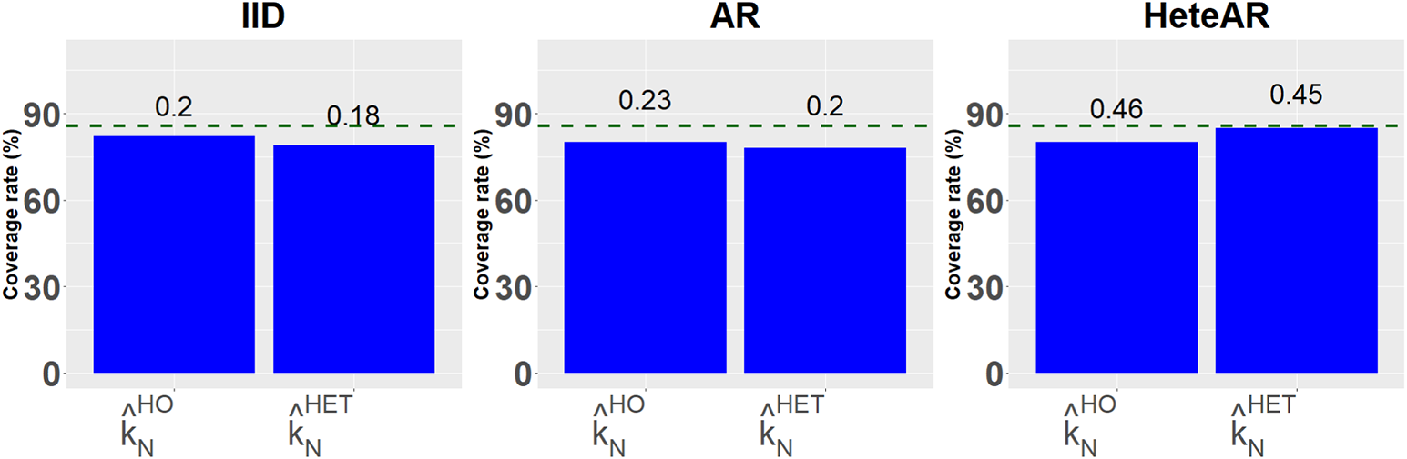
6 DATA APPLICATION
We present the results of data applications illustrating the use of the proposed confidence intervals and multiple change point estimation procedures.
6.1 Estimating the Changes in the New Keynesian Phillips Curve
In the first application, we focus on a recent topic of interest in the macroeconomic literature—the puzzle of the flattening Phillips curve in the United States. The relationship between the inflation and unemployment rate, depicted via the New Keynesian Phillips curve, has changed throughout U.S. economic history. Formally, the New Keynesian Phillips curve is
 $$ \begin{align*} \pi_i = \beta E_i \pi_{i+1} - \theta (u_i-u_i^{(n)}) + \nu_i, \end{align*} $$
where $\pi _i$
is the inflation,
$\pi _i$
is the inflation, $E_i \pi _{i+1}$
is the expected inflation at time
$E_i \pi _{i+1}$
is the expected inflation at time $i+1$
given the information up to time i, and
$i+1$
given the information up to time i, and $u_i$
and
$u_i$
and $u_i^{(n)}$
are, respectively, the unemployment rate and the natural rate of unemployment. The relationship between these two key macroeconomic variables can be easily captured by adapting the inflation expectation
$u_i^{(n)}$
are, respectively, the unemployment rate and the natural rate of unemployment. The relationship between these two key macroeconomic variables can be easily captured by adapting the inflation expectation $\beta E_i \pi _{i+1} = \pi _{i-1}$
. Thus, it yields the so-called accelerationist Phillips curve:
$\beta E_i \pi _{i+1} = \pi _{i-1}$
. Thus, it yields the so-called accelerationist Phillips curve:
 $$ \begin{align} \Delta \pi_i = -\theta (u_i - u_i^{(n)}) + \nu_i. \end{align} $$
Stock and Watson (Reference Stock and Watson2020) and Hazell et al. (Reference Hazell, Herreno, Nakamura and Steinsson2022) discuss the famous puzzle that the slope of the Phillips curve, $\theta $
, sharply drops from the early 1980s and flattens at
$\theta $
, sharply drops from the early 1980s and flattens at $-0.03$
in the sample from 2000 to the first quarter of 2019. Potential reasons for this are given in several papers. One of the main reasons discussed is structural changes (see, e.g., Peach, Rich, and Linder, Reference Peach, Rich and Linder2013; Tallman and Zaman, Reference Tallman and Zaman2017). For instance, technological developments, such as artificial intelligence, restrain wages and thus prices by making it easier to substitute capital for labor.
$-0.03$
in the sample from 2000 to the first quarter of 2019. Potential reasons for this are given in several papers. One of the main reasons discussed is structural changes (see, e.g., Peach, Rich, and Linder, Reference Peach, Rich and Linder2013; Tallman and Zaman, Reference Tallman and Zaman2017). For instance, technological developments, such as artificial intelligence, restrain wages and thus prices by making it easier to substitute capital for labor.
In this application, we use monthly data on core personal consumption expenditures (PCE), inflation, and the Congressional Budget Office (CBO) unemployment gap from Federal Reserve Economic Data, St. Louis website,Footnote 2 and examine the changes in the slope of the Phillips curve. In the linear model, the dependent variable is the year-over-year change (12-month backward-looking change) in the rate of core PCE, and we obtain the independent variable through the 12-month (backward-looking) moving average of the gap between the unemployment rate and the natural rate of unemployment. Our sample includes 737 observations from January 1961 to May 2022.
Following the simulation results in Section 5, we implement change point estimators and confidence intervals of $BP$
,
$BP$
, $ILR$
, and
$ILR$
, and $\hat {k}^{HET}_N(1/2)$
. Given the presence of several nuisance parameters, Algorithm 1 in Section F of the Supplementary Material outlines the procedure described in Section 2.2 for constructing confidence intervals for
$\hat {k}^{HET}_N(1/2)$
. Given the presence of several nuisance parameters, Algorithm 1 in Section F of the Supplementary Material outlines the procedure described in Section 2.2 for constructing confidence intervals for $\hat {k}^{HET}_N(1/2)$
. The data replication package in R is available at [https://github.com/yzhao7322/Confidence:Interval_Changes_in_Linear_Model].
$\hat {k}^{HET}_N(1/2)$
. The data replication package in R is available at [https://github.com/yzhao7322/Confidence:Interval_Changes_in_Linear_Model].
Figure 4 plots the estimated change points and confidence intervals on year-over-year core PCE inflation and CBO unemployment gap series. The dashed lines present a rolling window of size five years for the standard deviation of the model residuals, indicating the presence of heteroscedasticity. The estimators $BP$
and
$BP$
and $ILR$
identify common break dates in January 1974, April 1983, June 1992, and May 2002, while their confidence intervals differ.Footnote
3
In contrast, the method based on
$ILR$
identify common break dates in January 1974, April 1983, June 1992, and May 2002, while their confidence intervals differ.Footnote
3
In contrast, the method based on $\hat {k}^{HET}_N(1/2)$
uncovers changes in February 1975, August 1982, June 1988, and July 1996.Footnote
4
We estimate up to ten change points and use the BIC to eliminate redundant breaks. A notable feature of the confidence intervals is that they are wider on the more volatile side, as illustrated by the dashed line of the rolling-window standard deviation estimators, since the method accounts for heteroscedasticity.
$\hat {k}^{HET}_N(1/2)$
uncovers changes in February 1975, August 1982, June 1988, and July 1996.Footnote
4
We estimate up to ten change points and use the BIC to eliminate redundant breaks. A notable feature of the confidence intervals is that they are wider on the more volatile side, as illustrated by the dashed line of the rolling-window standard deviation estimators, since the method accounts for heteroscedasticity.
Plots of the year-over-year core PCE inflation and CBO unemployment gap data with the estimated change points and corresponding confidence intervals in the shaded areas, in which subfigures (a)–(c) present the results of $BP$
,
$BP$
, $ILR$
, and
$ILR$
, and $\hat {k}^{HET}_N(1/2)$
, respectively. The dashed lines show the rolling window estimators of the standard deviation of the residuals estimated from (6.1) with a rolling window of length
$\hat {k}^{HET}_N(1/2)$
, respectively. The dashed lines show the rolling window estimators of the standard deviation of the residuals estimated from (6.1) with a rolling window of length $w=60$
.
$w=60$
.
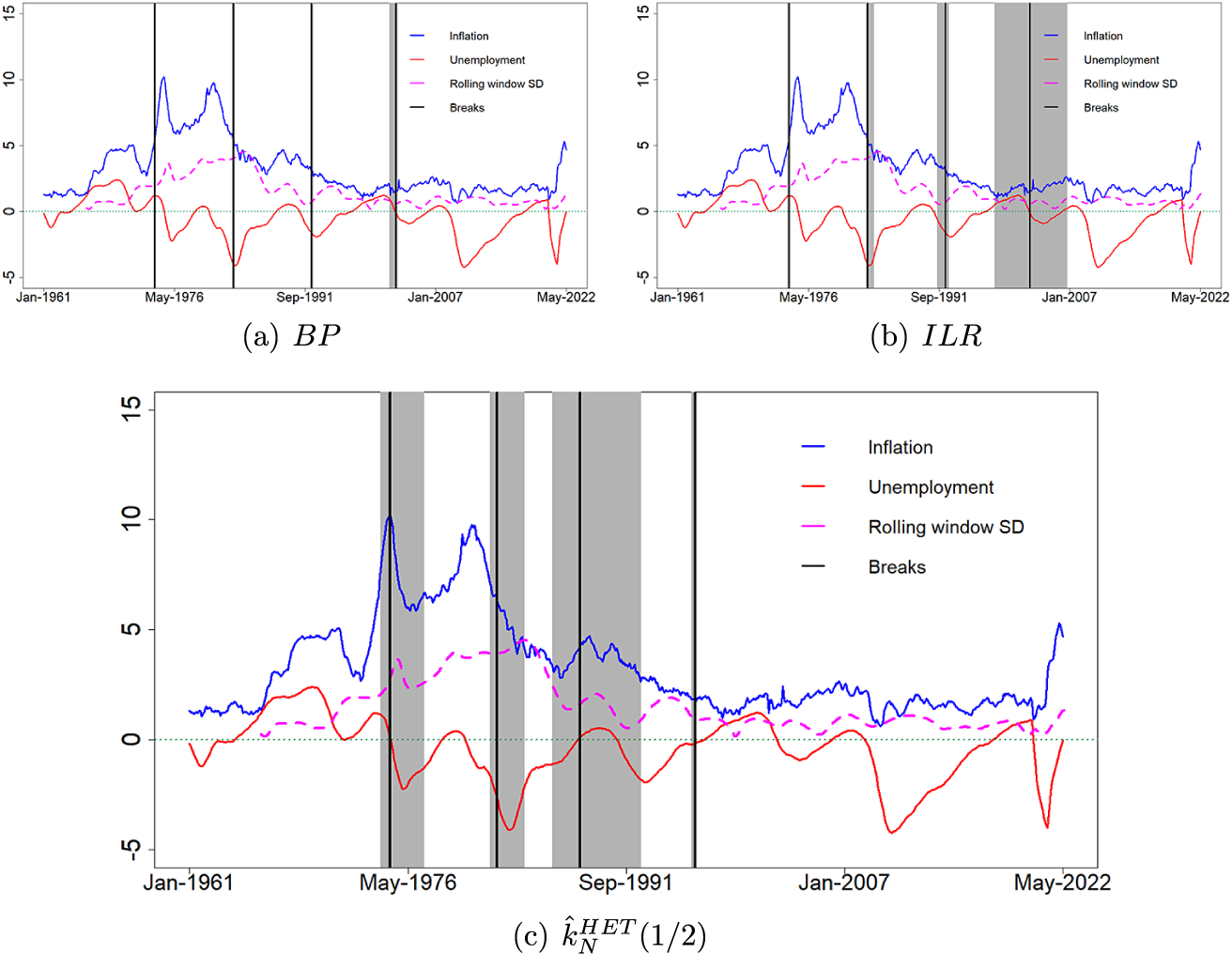
Next, we investigate the slope of the Phillips curve $\theta $
in each of the sub-samples segmented by the change point estimators. We document the slope and standard deviation estimators for
$\theta $
in each of the sub-samples segmented by the change point estimators. We document the slope and standard deviation estimators for $BP$
,
$BP$
, $ILR$
, and
$ILR$
, and $\hat {k}^{HET}_N(1/2)$
in each of their sub-samples (Table 2). We now summarize our findings. First, all three estimators suggest the first change around 1974–1975. The slope of the Phillips curve is unusually positive from the beginning of the sample until this break, reflecting the stagflation of the 1970s. Second, after the 1970s, all estimators indicate a flattening of the Phillips curve slope. For instance, the slope associated with
$\hat {k}^{HET}_N(1/2)$
in each of their sub-samples (Table 2). We now summarize our findings. First, all three estimators suggest the first change around 1974–1975. The slope of the Phillips curve is unusually positive from the beginning of the sample until this break, reflecting the stagflation of the 1970s. Second, after the 1970s, all estimators indicate a flattening of the Phillips curve slope. For instance, the slope associated with $BP/ILR$
declines from
$BP/ILR$
declines from $-2.60$
(February 1974–April 1983) to
$-2.60$
(February 1974–April 1983) to $-0.56$
(June 2002–May 2022), while
$-0.56$
(June 2002–May 2022), while $\hat {k}^{HET}_N(1/2)$
decreases from
$\hat {k}^{HET}_N(1/2)$
decreases from $-4.13$
(March 1975–August 1982) to
$-4.13$
(March 1975–August 1982) to $-0.44$
(August 1996–May 2022). These results align with the findings of Stock and Watson (Reference Stock and Watson2020) that the Phillips curve flattened around 2000. Comparatively, our method identifies breaks with decreasing magnitudes in coefficients, from
$-0.44$
(August 1996–May 2022). These results align with the findings of Stock and Watson (Reference Stock and Watson2020) that the Phillips curve flattened around 2000. Comparatively, our method identifies breaks with decreasing magnitudes in coefficients, from $-1.36$
to
$-1.36$
to $-0.44$
, toward the late 1980s and more recent periods, whereas the
$-0.44$
, toward the late 1980s and more recent periods, whereas the $BP/ILR$
model segments the sample into periods with similar slopes, around
$BP/ILR$
model segments the sample into periods with similar slopes, around $-0.46$
to
$-0.46$
to $-0.56$
, which may result from the presence of heteroskedastic errors. Lastly, our estimator
$-0.56$
, which may result from the presence of heteroskedastic errors. Lastly, our estimator $\hat {k}^{HET}_N(1/2)$
also detects a recent break in March 2020, which, however, is filtered out by the BIC criterion. Based on this change, we find that the Phillips curve exhibits a renewed negative slope of approximately
$\hat {k}^{HET}_N(1/2)$
also detects a recent break in March 2020, which, however, is filtered out by the BIC criterion. Based on this change, we find that the Phillips curve exhibits a renewed negative slope of approximately $-0.90$
, suggesting a partial restoration of its traditional relationship in the post-COVID-19 period.
$-0.90$
, suggesting a partial restoration of its traditional relationship in the post-COVID-19 period.
Estimated slope of the Phillips curve in five sub-samples obtained with $BP$
,
$BP$
, $ILR,$
and
$ILR,$
and $\hat {k}^{HET}_N(1/2)$
estimators
$\hat {k}^{HET}_N(1/2)$
estimators
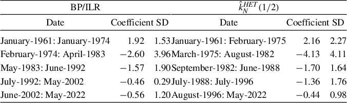
Note: SD is the standard deviation of the model residuals.
We conclude by noting that a second data application estimate confidence intervals for change points in linear models relating cryptocurrency to common risk factors is shown in Section H of the Supplementary Material.
7 CONCLUSION
This article proposes methods to detect change points and construct confidence intervals for them in linear regression models with heteroscedastic errors. Considering a heteroscedastic linear regression model with multiple changes in its coefficients, we introduce partial sum-type estimators based on the weighted residuals and establish their asymptotic behavior. These results can be used to construct confidence intervals for the times of changes. We further discuss binary segmentation and information criteria-based methods to determine the required preliminary estimators for the number and times of the change points. In a Monte Carlo simulation study, the empirical coverage rates of the estimated confidence intervals indicate that the proposed estimators perform well relative to competitors in finite samples. Additionally, adjustments for heteroscedasticity improve performance in models with heteroscedastic errors. Lastly, we apply the proposed method to construct confidence intervals for change points in the Phillips curve and cryptocurrency risk factors.
COMPETING INTEREST STATEMENT
The authors declare no competing interests exist.
FUNDING STATEMENT
The research of G.R. was supported by the Natural Science and Engineering Research Council of Canada’s Discovery and Accelerator grants.
SUPPLEMENTARY MATERIAL
Horváth, L., Rice, G., & Zhao, Y. (2026): Supplement to “Confidence intervals for multiple change points in linear models with heteroscedastic errors,” Econometric Theory Supplementary Material. To view, please visit: https://doi.org/10.1017/S026646662610036X.


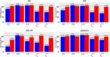


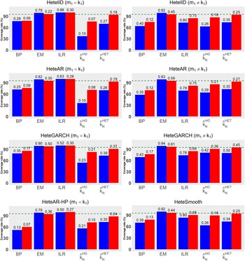


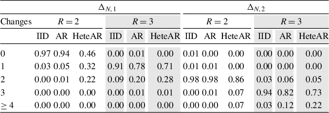


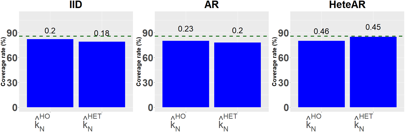


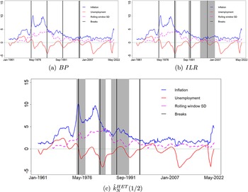


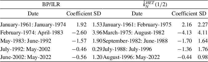


 Open access

