


Phyllosilicates are layer silicates whose layer unit is composed of an octahedral sheet (O; closed packed array of anions) linked to one or two tetrahedral sheets (T; near-hexagonal rings of tetrahedra). Three basic structures of layers are generally found: the so-called TO (1:1), TOT (2:1) and TOTO (2:1 + interlayer octahedral sheet) layers (Fig. 1a). Adjacent layers are linked by hydrogen bonds (e.g. TO minerals), by van de Waals forces (e.g. talc and pyrophyllite) or by various interlayer materials (hydrated cations, e.g. smectite; cations, e.g. mica; metal-hydroxyl octahedral sheets, e.g. chlorite). The assemblage of a layer plus interlayer is a unit structure and must be electrostatically neutral overall (e.g. Bailey, Reference Bailey, Brindley and Brown1981; Brigatti et al., Reference Brigatti, Malferrari, Laurora and Elmi2011). In the T sheet, the most common cations are Si, Al and Fe3+, whereas in the O sheet, the most common cations are Al, Mg, Fe3+ and Fe2+. Numerous other substitutions occur in natural and synthetic phyllosilicates (e.g. Kloprogge, Reference Kloprogge, Gates, Kloprogge, Madejová and Bergaya2017). When the octahedral cations are divalent, all octahedral sites are occupied and the structure is trioctahedral, whereas if octahedral cations are trivalent, only two-thirds of octahedral sites are occupied and the structure is dioctahedral (Fig. 1b). The position of (OH) in the dioctahedral sheet determines trans and cis octahedra (Fig. 1c). The plane layer cell is classically described by an (a,b) ortho-hexagonal cell in which the b parameter value (simply noted ‘b’ in the following) is equal to three times the distance between two adjacent octahedral cations. The structures of the O sheets are similar to those of hydroxide structures.
Schematic representation of (a) basic structures of TO, TOT and TOTO phyllosilicates. (b) Projection of a and b cell parameters (orthorhombic representation) on the surface of a trioctahedral and a dioctahedral sheet. (c) Distinction between cis- and trans-vacant di-octahedral sheets. (d) Tetrahedral rotation angle α.

To form a layer, similar lateral dimensions are required between the O and T sheets. In general, the lateral dimensions of the T sheet are larger than those of the O sheet, and a dimensional misfit occurs between these sheets. The T and O sheets can better form layers by contraction of T sheets via rotation of adjacent tetrahedra as measured by the α angle (Fig. 1d; e.g. Radoslovich & Norrish, Reference Radoslovich and Norrish1962; Bailey, Reference Bailey and Bailey1991b). An expansion of the lateral dimensions of the O sheet by flattening can better accommodate the linkage to the T sheet (e.g. Brigatti et al., Reference Brigatti, Galán, Theng, Bergaya and Lagaly2013). Other structural adjustments depending on the amount of strain at the sheet junction and the flexibility of the component O and T sheets can occur (e.g. Guggenheim & Eggleton, Reference Guggenheim and Eggleton1986). The degree of stress on the plane of the junction between O and T sheets greatly influences the resultant crystal size, morphology and structure of phyllosilicates (Bailey, Reference Bailey, Brindley and Brown1981).
Numerous authors have studied the correlations between the compositions of phyllosilicates and unit-cell parameters. The c parameter is particularly useful for phyllosilicates because in monoclinic unit cells the csin(β) = c* = d(001) corresponds to the ‘basal spacing’, or the layer-to-layer distance (Fig. 1a). The periodicity along c* can vary depending on the polytypic arrangement because of the different number of layers involved in the stacking sequence (e.g. Brigatti et al., Reference Brigatti, Malferrari, Laurora and Elmi2011). The b parameter is also of interest because it describes the O sheet lateral dimensions (Fig. 1b). Its value is obtained from X-ray diffraction (XRD) traces of the (06ℓ;33ℓ) reflections, with (060) giving b = 6.d(060). The d(060) value is commonly used to distinguish dioctahedral from trioctahedral phyllosilicates, the former ranging from 1.49 to 1.52 Å and the latter ranging from 1.52 to 1.53 Å (e.g. Środoń, Reference Środoń, Bergaya and Lagaly2013). Nontronite, a Fe3+-rich smectite, is an exception, with b superposed over the trioctahedral range (e.g. Petit et al., Reference Petit, Baron and Decarreau2017). b is sensitive to the octahedral site composition of phyllosilicates, and many correlations are available in the literature. For example, d(060) has been used to identify octahedral substitutions in kaolinite (e.g. Petit et al., Reference Petit1990). Brigatti (Reference Brigatti1983) correlated the octahedral site content of Fe and b of smectites (discussed below).
Most such results were presented as linear relationships (e.g. Russell & Clark, Reference Russell and Clark1978; Brigatti, Reference Brigatti1983; Petit et al., Reference Petit, Baron and Decarreau2017) between the b and octahedral site (and sometimes tetrahedral site) content. Many authors (e.g. Radoslovich, Reference Radoslovich1962; Rieder et al., Reference Rieder, Pichova, Fassova, Fediukova and Cerny1971; Wiewiora & Wilamowski, Reference Wiewiora and Wilamowski1996) used multiple regression equations such as in Equation 1:

where b 0 is the b cell parameter of the end member mineral with a i is the required regression coefficient for substituting cation i, and c i is the atomic content of cation i in the structural formulas (SFs) containing n types of substituting cations. These relations are restricted to a given family of phyllosilicates and do not allow generalized relationships. Hazen & Wones (Reference Hazen and Wones1972) established a clear correlation between the b of trioctahedral micas and the ionic radius of M 2+ octahedral-site cations. Similarly, Brindley & Kao (Reference Brindley and Kao1984) correlated the a and c unit-cell parameters of M(OH)2 hydroxides and M–O distances. Gerth (Reference Gerth1990) observed that the unit-cell b dimension varied with the ratio of metal-substituted goethite and was related to the ionic radii of incorporated metals. Bentabol & Ruiz Cruz (Reference Bentabol and Ruiz Cruz2013) examined the unit-cell values of lizardites with the ionic radius of the dominant M cations. However, for several M cations, the unit-cell values depend on the contribution of all octahedral cations (relative proportions and distribution). The current paper explores, in the light of the dimensional misfit between T and O sheets, the connection between the b of clay minerals and some related minerals with the mean ionic radius R of octahedral cations calculated as in Equation 2:

where r i is the ionic radius of octahedral cation i and x i is its molar fraction over n types of octahedral cations ($\mathop \sum \nolimits_{i = 1}^n ( {x_i} ) = 1$ ). Each family of minerals is discussed in this paper within a dedicated section that can be read separately.
Methods
Data for natural and synthetic samples were obtained from the literature. Most of the available b values were calculated from d(060) values measured from XRD unorientated powder traces according to the relation b = 6.d(060). The diffraction band at (060) is observed at 1.49–1.54 Å for clay minerals and represents several overlapping (06ℓ;33ℓ) reflections with small differences in d-spacing. Accordingly, differences between actual vs extracted b values are to be expected and must be considered for comparing data between measurement methods.
The d(hkl) values (in Å) derived from XRD experiments are generally given to ±0.005 Å, whereas the spot sizes in the figures represent the estimated uncertainties in the unit-cell parameters of samples. The mean ionic radius R of octahedral cations is calculated following Equation 2. Ionic radii are from Shannon (Reference Shannon1976; Table 1) and are given with ±0.01 Å uncertainty. SFs are from the literature or were calculated from chemical compositions. The uncertainty of R values cannot be generalized or estimated with accuracy. The data were selected carefully. For example, samples with SFs appearing to be obviously erroneous were disregarded.
Ionic radii (Å) of cations and O2– and their coordination from Shannon (Reference Shannon1976).

The b dimension of a theoretical ‘free’ T sheet (i.e. with hexagonal symmetry and no tetrahedral rotations) is b tet. = (4√2) × (Si–O) ≈ 9.15 Å, with an average bond length for Si–O = 1.618 ± 0.01 Å (Fig. 1d; Bailey, Reference Bailey, Brindley and Brown1981, Reference Bailey and Bailey1984b), and substitutions of larger cations for Si increase this value following Equation 3:

where x is the number of tetrahedral atoms substituted for Si (Si1–xIVTx). Accordingly, parameter a takes the value of 0.74, 1.26 or 1.15 for Al, Fe3+ or Ga, respectively. Be is treated as equivalent to Si in calculating b tet., as the Be–O bond length is close to that of Si–O (1.62 vs 1.618 Å, respectively). Equation 4 can be used to calculate α, the tetrahedral rotation angle, also termed ditrigonal rotation:

This unique relationship assumes that contraction occurs by tetrahedral rotation alone (e.g. Radoslovich & Norrish, Reference Radoslovich and Norrish1962), and it is not very accurate compared to structure refinement XRD single crystal data (Brigatti & Guggenheim, Reference Brigatti, Guggenheim, Mottana, Sassi, Thompson and Guggenheim2002). Clearly, for b/b tet. values >1, tetrahedral rotations do not apply because: (1) there are existing uncertainties in the bond lengths (e.g. the Si–O and IVAl–O bond lengths used are from Bailey (Reference Bailey and Bailey1984b) and are greater than those of Shannon (Reference Shannon1976)); (2) various other mechanisms are involved to adjust T and O sheet lateral dimensions; and (3) tetrahedral angles may vary. Accordingly, b/b tet., which also provides a measure of misfit (McCauley & Newnham, Reference McCauley and Newnham1971), was used here over the α value to compare samples. Moreover, Peterson et al. (Reference Peterson, Hill and Gibbs1979) estimated from semi-empirical molecular-orbital cluster calculations that a six-fold ring of a ‘free’ ideal T sheet has a minimum energy at α = 16° and not at α = 0°, suggesting that the ring has an intrinsic ditrigonal character irrespective of octahedral articulation.
Finally, the M–O bond lengths were calculated using R (Equation 2) as the average of the ionic radii in six-fold coordination (Table 1). For octahedral oxygen ions, coordination is (1) in four-fold for trioctahedral configuration (i.e. each oxygen ion is bonded to three M 2+ cations and one H+ ion) or (2) in three-fold for dioctahedral configuration (i.e. each oxygen ion is bonded to two M 3+ cations and one H+ ion). The b dimension of a theoretical ‘free’ O sheet (i.e. with regular octahedra) is$\;b_{{\rm oct}.} = 3\sqrt 2$ M–O (e.g. Guggenheim & Eggleton, Reference Guggenheim and Eggleton1987), and thus (Equation 5):

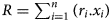
The percentage of octahedral enlargement (% O enlargement) corresponding to the difference between the calculated b oct. and observed b is according to Equation 6:

The % O enlargement reflects variations in O sheet lateral dimensions and is related to octahedral flattening and to O sheet thickness as described for micas by Toraya (Reference Toraya1981). An increase in the % O enlargement is related to an increase in octahedral flattening and a decrease in O sheet thickness. The % O enlargement vs R plot is another graphic representation of the R vs b plot that can be useful to discuss the variations in O sheet dimensions (Guggenheim & Eggleton, Reference Guggenheim and Eggleton1987) and O sheet thicknesses.
Results
Hydroxides, oxyhydroxides and layered double hydroxides
Hydroxides, oxyhydroxides and layered double hydroxides (LDHs; Fig. 2) require cell parameters to be transformed for comparison to phyllosilicates. Thus, to be equivalent to the b parameter of phyllosilicates, the hexagonal a of M(OH)2 hydroxides, the orthorhombic c of diaspore, the orthorhombic b cell parameters of other oxyhydroxides and the a of LDHs were each tripled. Table 2 provides the data used, which are plotted in Fig. 3 as a function of R.
Basic structure of (a) hydroxide (brucite), (b) oxyhydroxide (goethite) and (c) LDH.

Data used for hydroxide, oxy-hydroxide and LDH structures.

a, b and c are crystallographic parameters (Å).
R = mean ionic radius of octahedral cations (Å; see text for details).
a Sample reference in the paper.
b Using r(Mn3+) = 0.548 Å (see text).
c Extracted from Fig. 5.
d Single-crystal XRD measurement.
Evolution of the equivalent b parameter (in Å) with the mean ionic radius of octahedral cations R (in Å) for hydroxide families (Table 2). (a) Mn +(OH)n hydroxides: square = natural gibbsite; triangles = M 2+-hydroxide synthetic series. (b) MO(OH) oxyhydroxides, with squares and triangles corresponding to natural and synthetic samples, respectively: black = diaspore; red = goethite; green = groutite; dark blue = GaO(OH); light blue = Ga-goethite series; orange = Co3+-, Ni2+-, Cu2+-, Zn2+-, Cd2+- and Pb4+-goethite series; pink = Al-goethite series; green = Mn3+-goethite series; brown = Cr3+-goethite series. (c) LDHs, with squares and triangles corresponding to natural and synthetic samples, respectively: light blue = MgAlCO3; green = NiAlCO3; light green = MgFeCO3; orange = NiFeCO3; pink = CoAlCO3; violet = CoFeCO3; dark blue = GaM 2+CO3; yellow = CoCuAlCO3; brown = others. (d) Comparative regressions calculated from the model between the octahedral sheet dimension and R (see text for details): blue dotted line = Mn +(OH)n; green dotted line = MO(OH); red dotted line = LDHs.

The plots for synthetic M 2+(OH)2 brucite-like hydroxide structures (Fig. 2) with M = Mg, Ni, Co, Fe, Mn, Cd and Ca are in excellent agreement with the b vs R correlation (Fig. 3a). The relation, b = 4.4878R + 6.2462, is consistent with Brindley & Kao (Reference Brindley and Kao1984). Moreover, the M 2+(OH)2 minerals plus gibbsite fall on the same correlation line with a very high R 2 (0.996). In gibbsite, each octahedron is distorted, and the vacant site has the greatest size (Saalfeld & Wedde, Reference Saalfeld and Wedde1974). As b conforms to the mean ionic radius of either di- or trivalent actual octahedral cations, the contribution of the vacant site is integrated within R.
For MO(OH) oxyhydroxides (Figs 2 & 3b), a unique regression was derived for the group except for M = Mn3+ (see below), yielding the relation b = 4.6673R + 6.0546. Diaspore (Al), goethite (Fe3+), synthetic GaO(OH) end members and synthetic goethite substituted by heterovalent (divalent, tetravalent) cations are in good agreement with the regression. Except for Ga3+, cation substitution is very limited in goethite (Table 2). For example, Stiers & Schwertmann (Reference Stiers and Schwertmann1985) failed to synthesize the complete Fe3+–Mn3+ goethite solid solution and achieved ≤15% Mn3+ (Table 2). Groutite (α-MnOOH), which is isostructural with goethite, has an orthorhombic b of ~2.87 Å, but this is ~3.02 Å for goethite (Table 2), although r(Mn3+) is identical to r(Fe3+) (Table 1). Because of Jahn Teller effects (Shannon et al., Reference Shannon, Gumerman and Chenavas1975), octahedra are distorted strongly in groutite, with four short Mn–O distances (two of 1.895 Å and two of 1.965 Å) and two long Mn–O distances (2.174 and 2.338 Å), with a mean Mn–O distance of 2.039 Å (Kohler & Armbruster, Reference Kohler and Armbruster1997). Assuming this mean Mn–O distance and r(O2–) = 1.36 Å, the mean r(Mn3+) would be 0.679 Å, which cannot account for the large difference in the equivalent b between groutite and goethite. When using the regression obtained for MO(OH) structures (Fig. 3b), the b for groutite corresponds to an ‘effective’ r(Mn3+) = 0.548 Å. Using this ‘effective’ r(Mn3+), the synthetic Mn-goethites (Stiers & Schwertmann, Reference Stiers and Schwertmann1985) follow the regression well (Fig. 3b), and the R 2 of the regression was slightly greater when the Mn3+ data were included (0.9845 vs 0.9818). This suggests that in the groutite structure b is mainly dependent on the shortest Mn–O distances.
The LDH structure is based on brucite Mg(OH)2 with octahedral coordination around the metal ions (Fig. 2). Substitutions of divalent M 2+ cations by trivalent M 3+ cations produce many isostructural materials with the general formula M 2+1–xM 3+x(OH)2An –x /n,yH2O (Table 2). These layered materials are readily synthesized (e.g. Forano et al., Reference Forano, Costantino, Prévôt, Taviot Gueho, Bergaya and Lagaly2013) and have numerous applications (e.g. Choi et al., Reference Choi, Oh and Choy2008; Costantino et al., Reference Costantino, Nocchetti, Sisani and Vivani2009). Studying natural as well as synthetic hydroxy-carbonates, Brindley & Kikkawa (Reference Brindley and Kikkawa1979) observed a very good correlation between the a parameter and the extent of Al/M 2+ substitution, but they considered the Mg–Al and Ni–Al systems separately. Using the mean ionic radius R of octahedral cations, the cell parameters can be compared, regardless of the elemental composition of the LDHs, and this leads to the relation b = 4.2043R + 6.3758 (Fig. 3c). The lower value of the regression coefficient for the LDH minerals compared to the other hydroxides may be related to uncertainties in their more complex chemical composition. Indeed, because LDHs are synthesized under pH conditions in which cations can precipitate, bulk chemical analyses would give elemental compositions consistent with the elemental composition of the starting solution. However, the coprecipitation of amorphous or nanocrystalline phases cannot be excluded and may be barely detectable using conventional analytical methods, so that the true elemental composition of LDH phases may be different from the expected composition. Chemical analyses obtained using transmission electron microscopy coupled to an energy-dispersive X-ray detector would thus give more reliable results, as the elemental composition and its dispersion through the sample are good indicators of the purity of the studied samples. As an example, for the shigaite natural sample, which was found relatively far from the range (Fig. 3c), the calculated value for the M 2+:M 3+ ratio using the correlation equation would be 2.57 instead of 2.00 (i.e. 2.16 for the number of Mn2+ atoms instead of 2).
The regressions between the O sheet dimensions and R for the three types of hydroxide families have similar slopes (Fig. 3d), despite their different crystallographic structures, implying that the O sheet dimension depends essentially on the shape and size of neighbouring octahedra. The effect of the octahedral composition on the distance between two octahedral cations located in two adjacent octahedra is similar for Mn +(OH)n, MO(OH) and LDHs, regardless of the di- or trioctahedral character of the minerals. For the same R, the octahedral dimension of Mn +(OH)n hydroxide minerals is slightly greater (0.08 ± 0.005 Å) than those of the two other structures that are more constrained due to their greater complexity (Fig. 3d). The impact of structure is similar for oxy-hydroxides and LDHs in the existing compositional range.
Brindley & Kao (Reference Brindley and Kao1984) showed that the octahedral sheets in trioctahedral brucite-like structures are all flattened to the same extent with a mean flattening angle τ = O–M–O, with O in the same plane varying slightly from 97.1° to 98.1° (average 97.4°). The unique linear regression observed here between gibbsite and trioctahedral hydroxides suggests that τ is similar for gibbsite and for all Mn +(OH)n hydroxides. Accordingly, from refined structures, the values of the flattening angle τ were found to be 98.5° and 98.3° for gibbsite (Saalfeld & Wedde, Reference Saalfeld and Wedde1974) and brucite (Parise et al., Reference Parise, Leinenweber, Weidner, Tan and von Dreele1994), respectively.
The structure of Mn +(OH)n hydroxides approximates a hexagonally close-packed arrangement of anions with Mn + ions in octahedrally coordinated positions between alternating pairs of anion planes. The b used here is given by b = 6(M–O)sin(τ/2), with the (M–O) distance being the sum of the effective ionic radii for cations (M) in six-fold coordination and oxygen ions (O) in four-fold coordination (r(IVO2–) = 1.38 Å; Table 1; Brindley & Kao, Reference Brindley and Kao1984). Using the mean ionic radius of octahedral cations R, this relation can be easily rewritten as b = 6(R + 1.38)sin(τ/2).
Following a structurally based interpretation, a relation b = AR + C can be obtained for each family of hydroxides studied here using a simple model with A = 6sin(τ /2) and C = A1.38 (in Å). The A (and thus τ and C) were determined by fitting with the experimental regressions (Fig. 3d).
For Mn +(OH)n hydroxides, A and C are 4.51 and 6.22, respectively (Fig. 3d), close to the experimental values derived from the correlation line shown in Fig. 3a (4.49 and 6.25, respectively). The corresponding τ = 97.3° agrees well with the literature (see above). The corresponding % O enlargement (or octahedral flattening) is ~6.3%.
The proposed model for Mn +(OH)n hydroxides is also suitable for MO(OH) and LDHs, as seen in Fig. 3d, where the A values are very close for MO(OH) and LDHs, at 4.47 and 4.48, respectively. The octahedra are slightly less flattened in MO(OH) and LDHs compared to Mn +(OH)n hydroxides, with τ = 96.3° (~5.4% octahedral enlargement) for MO(OH) and τ = 96.6° (5.6% octahedral enlargement) for LDHs.
The structurally based model of the hexagonally close-packed arrangement of anions with Mn + ions in octahedrally coordinated positions shows very good efficiency in reconciling structural and chemical data for all families of studied hydroxides as well as for both di- and trioctahedral minerals (Fig. 3d), and the relation between the equivalent b and the mean ionic radius of octahedral cations R for each mineral allows us to measure the flattening of octahedra, which is similar for all of the families and does not vary significantly within each family.
TO phyllosilicates
TO phyllosilicates are composed of the superimposition of a T sheet of a pseudo-hexagonal ring of (SiO4)4– units on an O sheet of edge-sharing octahedra leading to an electrostatically neutral layer (Fig. 1a). The general SF is (SiaR 3+b)2(R 3+cR 2+d□e)3O5(OH)4, with R 3+ being mainly Al and Fe3+, R 2+ being mainly Mg (but this could other divalent cations, such as Ni and Fe2+) and □ being a vacant site. Anions other than OH–, such as F– or Cl–, are rarely reported as occurring and will not be discussed here. Kaolins and serpentines constitute the dioctahedral and trioctahedral families, respectively. Kaolin group minerals include kaolinite, dickite, nacrite and halloysite and have a general composition of Al2Si2O5(OH)4 (+ nH2O for halloysite), with similar b values (Giese, Reference Giese and Bailey1991) and very few substitutions. Consequently, only kaolinite was considered in the following as a representative of the whole kaolin group.
Contrary to kaolins representing Al end members with no tetrahedral substitutions and a very simple chemical composition, serpentines display a wide range of chemical compositions, leading to many end members depending on the extent of the tetrahedral substitutions and the nature of the dominant octahedral cations. For instance, lizardite (Mg) and nepouite (Ni; a ≈ 2 and d ≈ 3), berthierine (b ≈ 0.5, c ≈ 0.5 and d ≈ 2.5), brindleyite (b ≈ 0.5, c ≈ 1, d ≈ 1.75 and e ≈ 0.25) and amesite (Al–Mg) and cronstedtite (Fe3+, Fe2+; b ≈ 1, c ≈ 1 and d ≈ 2) represent different minerals of these serpentine families (Wiewiora, Reference Wiewiora1990). Three structural groups of serpentines based on particle shape are also distinguished: flat layers as for lizardite (Fig. 4a), cylindrical layers as for chrysotile (Fig. 4b) and corrugated layers as for antigorite (Fig. 4c; e.g. Wicks & Whittaker, Reference Wicks and Whittaker1975), and many morphologies have been reported (e.g. Andreani et al., Reference Andreani, Grauby, Barronnet and Munoz2008).
Schematic representation of various structures of TO serpentines based on crystal morphology: (a) flat morphology, (b) curved morphology and (c) wavy corrugated morphology.

Kaolinite and lizardite
Kaolinite and lizardite are the Al-dioctahedral and Mg-trioctahedral end members, respectively, for TO phyllosilicates having the general SF of Si2(R 3+cR 2+d)O5(OH)4. For the kaolinite dioctahedral end member, c and d are 2 and 0, respectively, and R 3+ is Al, while for the lizardite trioctahedral end member, c and d are 0 and 3, respectively, and R 2+ is Mg. No or limited octahedral substitutions (mainly Fe3+ for Al3+) occur in natural kaolinite. Using the synthesis method, the Fe3+ substitution amount can be increased slightly and other octahedral cations can be introduced into the structure (Table 3). Among the large set of published data available for pure natural Al end member kaolinite, the Keokuk kaolinite studied using Rietveld refinement (Bish &Von Dreele, Reference Bish and Von Dreele1989) was selected as representative for this study. According to the general SF above, lizardite sensu stricto does not have tetrahedral substitutions. Consequently, in this study, lizardite with >0.1 IVAl was considered in the Al-serpentine series rather than in the lizardite series.
Data used for TO phyllosilicates.

b is a crystallographic parameter (Å).
R = mean ionic radius of octahedral cations (Å; see text for details).
a Sample reference in the paper.
b Brindley (Reference Brindley1982).
c Brindley et al. (Reference Brindley, Dunham, Eyles and Taylor1951).
d Calculated from chemical analyses in Brindley et al. (Reference Brindley, Dunham, Eyles and Taylor1951).
e Crystal structure refinement.
f Average value.
g Caryopilite.
As shown in Fig. 5a, the b vs R plots for all TO samples display a relatively scattered pattern. Two different regressions (i.e. the kaolinite–lizardite (K–L) and greenalite–caryopilite (G–C) lines) can be distinguished, however, with a wide cloud of dots at their intersection (Fig. 5a).
b vs mean ionic radius of octahedral cations R for TO phyllosilicates (Table 3). (a) Circles represent natural samples and triangles represent synthetic samples: dark blue = kaolinite; yellow = lizardite; black = antigorite; light green = Al-serpentine, with black border = brindleyite, open circle = kellyite; red = Fe3+-serpentine, full circles = cronstedtite, with black border = pecoraite, open circles = guidottite; dark green = greenalite; brown = caryopilite; violet = R 2+-chrysotile series; pink = Co-lizardite. (K–L) and (G–C) correspond to kaolinite–lizardite and greenalite–caryopilite regression lines, respectively. (b) Focus on the synthetic kaolinite–lizardite series: dark blue triangles = Fe3+-kaolinite series, open triangle = theoretical end member; light blue triangle = Ga3+-substituted kaolinite; red triangles = R 3+-kaolinite series; yellow triangles = Ni–Mg lizardite series; pink triangles = Co-lizardite; open violet triangles = R 2+-chrysotile; light green triangles = Mg–Al serpentine series (Chernosky, Reference Chernosky1975), open light green triangles = other Mg–Al serpentines; brown triangles = R 2+–Al serpentine series; green triangle = greenalite. (c) Focus on natural Al-serpentines (circles) and Fe3+-serpentines (triangles). Polytype (partly) and tetrahedral Al or Fe3+ pfu are indicated: light blue circles = amesite; orange circles = berthierine, orange open circle = Ti-berthierine; green open circle = brindleyite; pink circles = odinite; dark blue circle = kellyite; green circles = other; red triangles = cronstedtite (2H 1, 2H 2, 3T, 1T, 6T 2 and 3T + 1M polytypes); blue triangle = pecoraite; green triangles = guidottite.

Natural kaolinite, the synthetic Al–Fe3+ kaolinite series and the synthetic Ni–Mg lizardite series appear quasi-aligned ((K–L) line in Fig. 5a,b). The (K–L) line was first calculated with the synthetic series of Fe3+-kaolinites (Petit et al., Reference Petit1990; Iriarte et al., Reference Iriarte, Petit, Huertas, Fiore, Grauby, Decarreau and Linares2005) and Ni–Mg lizardites (Baron et al., Reference Baron, Pushparaj, Fontaine, Sivaiah, Decarreau and Petit2016b; Fig. 5a,b). Including natural kaolinite in these two synthetic series increases the correlation coefficient slightly (0.9987 instead of 0.9985) without modifying the regression significantly (b = 1.5092R + 8.1371 instead of b = 1.5097R + 8.1368). The K–L regression including the natural kaolinite was kept in the following analyses. Because aluminium is the octahedral cation with the smallest ionic radius (0.535 Å; Table 1), the b of the pure Al end member exhibits the smallest value observed for TO phyllosilicates when forming a TO clay structure. Accordingly, the natural Keokuk pure kaolinite is located at the origin of the regression line with an R value of 0.535 Å and a b value of 8.945 Å according to Bish & Von Dreele (Reference Bish and Von Dreele1989). Few b values for synthetic Fe3+- and Ga3+-substituted kaolinites of Bentabol et al. (Reference Bentabol, Ruiz Cruz and Huertas2009) are lower than 8.945 Å (Fig. 5b & Table 3), suggesting an underestimation of these b values. The data for the kaolinite synthesized with the greatest Cr3+ content also deviate slightly from the correlation lines (Fig. 5b). Except for the samples described in Bentabol et al. (Reference Bentabol, Ruiz Cruz and Huertas2009), the dataset for other synthetic diversely substituted kaolinites is located on or close to the regression line (Fig. 5b).
Up to ~0.1 octahedral Fe3+ per formula unit (pfu) is observed in natural kaolinites, whereas up to 0.6 substituted Fe3+ pfu can be measured in synthetic kaolinites (Table 3). For the theoretical Fe3+-kaolinite end member (Si2Fe3+2O5(OH)4), b extrapolated using the experimental data from Iriarte et al. (Reference Iriarte, Petit, Huertas, Fiore, Grauby, Decarreau and Linares2005) is located close to the K–L regression line, supporting the suitability of the dataset for a wide range of compositions (Fig. 5b). Moreover, as concluded previously by some authors (Petit et al., Reference Petit, Decarreau, Eymery and Thomassin1988; Petit & Decarreau, Reference Petit and Decarreau1990; Iriarte et al., Reference Iriarte, Petit, Huertas, Fiore, Grauby, Decarreau and Linares2005), the Al–Fe3+ kaolinite synthetic series behaves like a solid solution within the compositional range explored, and no evidence exists to date to suggest that the maximum value obtained experimentally (0.6 pfu) corresponds to a steric limit of Fe3+ substitution in kaolinite.
In contrast to kaolinite, various end members of lizardite are encountered, and Mg cations are commonly replaced at least partially by other divalent cations (Table 3). As shown in Fig. 5b, the synthetic Mg–Ni lizardites are well aligned on the (K–L) line, The Co-lizardite does not fit the regression well. The two different b values were measured in the same sample, as Bayliss (Reference Bayliss1981) calculated a significantly greater b than that measured by Dalmon & Martin (Reference Dalmon and Martin1968; Fig. 5b). The deviation from the (K–L) regression line and the b fluctuations probably suggest there being a problem with these data. In a review of serpentine group minerals, Bayliss et al. (Reference Bayliss, Berry, Mrose and Smith1980) observed some significant fluctuations in reported b values with apparently the same chemistry, suggesting different methods had been employed to measure this parameter or inaccuracies had occurred during these measurements. Fluctuations are noticed for synthetic Mg end members, with b ranging from 9.204 to 9.241 Å (Table 3). Fluctuations are also observed for natural lizardites whose single-crystal XRD refinement of two different crystals from a same sample with an assumed homogeneous chemical composition resulted in two different b values, as illustrated by the Gew-graze lizardite-1T (Mellini et al., Reference Mellini, Cressey, Wicks and Cressey2010) and the Monte Fico lizardite-1T (Mellini & Viti, Reference Mellini and Viti1994; Table 3). More consistent with the results observed here, Mellini & Zanazzi (Reference Mellini and Zanazzi1987) measured a slight variation in b coupled with a slight variation in the chemical composition between two polytypes of the Coli lizardite sampled within the same vein (Table 3). These examples illustrate how the established correlation lines can help us to identify whether deviation originated from structural features or difficulties in accurately measuring b.
Lizardite, chrysotile and antigorite are three polymorphs with flat, curved and corrugated wavy layer structures, respectively. Antigorite corresponds to a polysomatic series, with regularly inversed T sheets in polysomes (Fig. 4). A more correct general formula for antigorite would then be (Mg)3m–3Si2mO5m(OH)4m−6, where m represents the number of tetrahedra within a full wavelength, and m = 17 has been proposed as the most common value (Capitani & Mellini, Reference Capitani and Mellini2004). The dataset does not allow for the identification of possible differences between the polymorphs. As far as synthetic Mg- and Ni-lizardites (Baron et al., Reference Baron, Pushparaj, Fontaine, Sivaiah, Decarreau and Petit2016b) and chrysotiles (Jasmund et al., Reference Jasmund, Sylla, Freund and Bailey1976) are concerned, b values measured for chrysotiles appear slightly lower than those measured for lizardites (Table 3). Because the two sets of samples were measured using various techniques, we cannot conclude with certainty that b values for chrysotiles are lower than for lizardites.
Al- and Fe3+-serpentines
Al- and Fe3+-serpentines whose general SFs are (Si2–xAlx)(Mg3–xAlx)O5(OH)4 and (Si2–xFe3+x)(Fe3+xFe2+3–x)O5(OH)4, respectively, most often exhibit great tetrahedral substitution contents (up to 1 Al or Fe3+ per O5(OH)4) to neutralize the positive octahedral layer charge generated by the heterovalent octahedral substitutions of divalent cations (mainly Mg and Fe2+) by trivalent cations (mainly Fe3+ and Al). The dataset for Al- and Fe3+-serpentines are scattered significantly (Fig. 5a), and this scattering is more pronounced for natural samples than for synthetic Al-serpentines, which lie close to the (K–L) regression line (Fig. 5b). The natural Al- and Fe3+-serpentines exhibit a wide range of tetrahedral substitutions and several polytypes, but no specific trend can be observed between these two characteristics and b (Fig. 5c).
Greenalite and caryopilite
Greenalite and caryopilite are, respectively, Fe2+- and Mn-rich TO phyllosilicates with corrugated structures and with the following general SF: Si2(M)(2.5–3)O5(OH)4, with M = Fe, Mn, Mg and Al as the main octahedral cations. Partial oxidation of octahedral Fe and Mn often occurs, and some octahedral sites may be vacant. The regression parameters for the (G–C) line (Fig. 5a) and the structural interpretation are discussed in detail below. The slope of the (G–C) regression line is ~4.5 times greater than that of the (K–L) line. Jasmund et al. (Reference Jasmund, Sylla, Freund and Bailey1976) reported that the greenalite synthesized with the Fe2+ end member was structurally non-equivalent to the Ni-, Mg- and Co-lizardites. The observed scattering of samples around the (G–C) line (Fig. 5a) can be tentatively assigned to uncertainties in the data and/or to the various modulated local substructures. Greenalite and caryopilite exhibit domed island-like structures due to tilting of the tetrahedra with periodic inversions of three- and four-fold rings (Guggenheim & Eggleton, Reference Guggenheim and Eggleton1998). This structural adjustment is a way to enlarge the T sheet dimensions to allow congruence with the large O sheet dimensions due to the occurrence of significant amounts of octahedral cations with large ionic radii, such as Mn2+ and Fe2+ (Table 1).
Influence of tetrahedral composition
Whereas no relation can be observed between tetrahedral content and b as shown above (Fig. 5c), it is clear, however, from a simple comparison between, for example, Mn-rich serpentines (i.e. kellyite; IVAl-serpentine, guidottite (IVFe3+-serpentine) and caryopilite (negligible tetrahedral substitution and corrugated structure), that the tetrahedral composition plays a role in the dimensional misfit between T and O sheets. All of these Mn-rich serpentines have great R (from ~0.73 to ~0.80 Å) and b values (from ~9.4 to ~9.8 Å) due to their great Mn content. The tetrahedral substitutions in kellyite and guidottite allow the lateral dimension of the T sheet to increase, making the fit between T and O sheets possible without corrugation of the layer.
The b/b tet. values were calculated for all TO phyllosilicates and plotted as a function of R (Fig. 6a). Three general trends are observed. The (K–L)’ correlation line (Fig. 6a) corresponds to the (K–L) line (Fig. 5a), and the regression was calculated using the same data. These samples have no tetrahedral substitutions and thus the correction with the b tet. value does not influence the data alignment (Fig. 6a). Note that the synthetic R 2+–Al serpentine samples (Bentabol & Ruiz Cruz, Reference Bentabol and Ruiz Cruz2013) that were above the (K–L) line (Fig. 5a,b) are now closer to the (K–L)’ line (Fig. 6a). The odinite data deviate systematically from the trend (Figs 5a & 6a), and possible impurities and redox variation make their SF unsure. Compared to the b vs R plot (Fig. 5a), the cloud of dots associated with the Al-serpentine disappeared in Fig. 6a. Less predictable is that the corrugated Fe2+–Mn serpentines approximately follow the same high-slope (G–C)’ line as most of the Al-serpentines (Fig. 6a). For this (G–C)’ line, the regression was calculated using antigorites, greenalites, caryopilites and Al-serpentines that are on (or close to) the (G–C)’ line. Furthermore, the Fe3+-serpentines, except the pecoraite sample, which lies on the (G–C)’ line, follow fairly well the different linear trend of (Fe3+–Serp)’ with the same slope as the (G–C)’ line (Fig. 6a).
(a) b/b tet. ratio vs mean ionic radius of octahedral cations R for TO phyllosilicates (Table 3), with the same symbols and colours as in Fig. 5a. (K–L)’ and (G–C)’ correspond to kaolinite–lizardite and greenalite– caryopilite regression lines, respectively. (b) Evolution of the percentage of octahedral enlargement compared to hydroxides (Equation 6; see text for details) vs R: blue squares = kaolinites and lizardites; green squares = natural Al-serpentines; green triangles = synthetic Al-serpentines (focus on the Chernosky's (Reference Chernosky1975) series); red squares = Fe3+-serpentines; black squares = antigorite; brown squares = caryopilites and greenalites; blue dotted line = regression for the kaolinite–lizardite series. (c) Evolution of the percentage of octahedral enlargement vs b tet. for Al- and Fe3+-serpentines, with the same symbols and colours as in Fig. 5c for natural samples, except light green crosses = synthetic Al-serpentines.

For Al- and Fe3+-serpentines, a general relationship of b vs R, introducing the tetrahedral composition, can be formulated from each (K–L)’, (G–C)’ and (Fe3+–Serp)’ regression line (Fig. 6a) according to Equation 7:

with T being the number of IVAl or IVFe3+ pfu.
For Al-serpentines following the (K–L)’ line (Fig. 6a):

For Al-serpentines (and Fe3+-serpentine; i.e. pecoraite) following the (G–C)’ line (Fig. 6a):

For Fe3+-serpentines following the (Fe3+–Serp)’ line (Fig. 6a):

The intersect coordinates for the two (K–L)’ and (G–C)’ lines are R = 0.717 and b = 9.220 Å, approximately corresponding to the Mg-lizardite end member. The corresponding b/b tet. value is 1.007, thus indicating a tetrahedral rotation angle α close to 0°. Accordingly, theoretical modelling using the distance least-squares method indicates that the O and T sheets fit together without any major distortions in the Mg-lizardite structure (Bish, Reference Bish1981; Wicks & Hawthorne, Reference Wicks and Hawthorne1986; Wicks & O'Hanley, Reference Wicks, O'Hanley and Bailey1991), and α measured using structure refinement is close to 0° (approximately –1.5(1)°) for the natural Mg end member lizardite (Guggenheim & Zhan, Reference Guggenheim and Zhan1998; Mellini et al., Reference Mellini, Cressey, Wicks and Cressey2010).
Based on all of the results above, three main distinct mechanisms of adjustment between O and T sheet lateral dimensions to compensate for the misfit of kaolinite–lizardite, Al- and Fe3+-serpentines and phyllosilicates with corrugated structure are proposed in the following subsections.
Focus on the structural adjustment mechanism for the kaolinite–lizardite family
Samples on the (K–L)’ line (Fig. 6a) are those for which b is driven by R according to the good regression observed for the (K–L) line (Fig. 5a). For pure kaolinite (Al end member that exhibits the lowest R), T sheets are relatively large compared to O sheets and have to reduce their lateral dimensions to adjust to the O sheets. Moving to lizardite, and thus increasing R, makes the dimensional misfit decrease. The (K–L)’ trend (Fig. 6a) gives evidence of a progressive decrease of the angle of tetrahedral rotation α with increasing R. Accordingly, the rotation of tetrahedra to ditrigonal symmetry (Fig. 1d) is the principal process for overcoming the misfit when b oct. < b tet. in TO phyllosilicates by reducing the lateral dimension of the T sheet (e.g. Radoslovich, Reference Radoslovich1963; Bailey, Reference Bailey and Bailey1966; Wicks & Whittaker, Reference Wicks and Whittaker1975; Guggenheim & Eggleton, Reference Guggenheim and Eggleton1987). However, this process is not the only one to achieve congruency between the T and O sheet dimensions. Indeed, the O sheet enlargement (Equation 6) increases progressively with a decrease of R (Fig. 6b). The O sheet enlargement corresponds to a lateral expansion of the sheet by thinning (Bailey, Reference Bailey and Bailey1984b). The b oct. value corresponding to an unconstrained O sheet was taken for hydroxides as determined above (b oct. = 4.51R + 6.22; Fig. 3d). Consequently, positive % O enlargement corresponds to an O sheet flattening (or thinning) compared to hydroxides, whereas negative % O enlargement corresponds to a thickening of the O sheet compared to hydroxides, with a null value being obtained for R = 0.642. With the ionic radius of Fe3+ being 0.645 Å (Table 1), the theoretical Fe3+-kaolinite end member would have similar dimension to the corresponding hydroxide. The Fe(OH)3 mineral bernalite exists but it has a pseudo-cubic structure of perovskite type (Birch et al., Reference Birch, Pring, Reller and Schmalle1993) that cannot be compared. Kaolinite exhibits the greatest enlargement: 3.6% as compared to hydroxides (10.1% as compared to undistorted O sheets), which agrees well with the value measured using structure refinement (10.1%; Bish & Von Dreele, Reference Bish and Von Dreele1989). Co-lizardite with the lowest octahedral enlargement (–3.7% and 2.3% compared to hydroxides and undistorted O sheets, respectively) and has the thickest O sheet of the family. The linear regression observed between kaolinite and lizardite (Fig. 6b & (K–L) line Fig. 5a) suggests an increase of the size of the vacant site with an increase of R for dioctahedral samples.
The few Al- and Fe3+-serpentines with a rather low rate of tetrahedral substitution that lie on (or close to) the (K–L)’ line (i.e. brindleyite, pecoraite and synthetic R 2+–Al serpentines; Fig. 6a) behave similarly to the kaolinite and lizardite family. These Al-serpentines exhibit a great number of octahedral vacant sites, possibly increasing the plasticity of the octahedral sheet compared to the other serpentines.
Focus on the Al- and Fe3+-serpentines family
The samples that are scattered between the (K–L) and (G–C) lines exhibit a high degree of misfit due to their relatively small O sheet lateral dimensions (small R) compared to their large T sheet lateral dimensions due to tetrahedral substitutions. The T sheet dimensions have to decrease significantly to adjust to the O sheet. As for kaolinite and lizardite, this reduction of T sheet dimensions with decreasing R is due to a progressive increase in the tetrahedral rotation angle α, as evidenced by the (G–C)’ and (Fe3+–Serp)’ regressions (Fig. 6a). However, contrary to the kaolinite–lizardite series, the O sheet enlargement does not vary linearly with R and is relatively more pronounced than for kaolinite–lizardite (Fig. 6b). This explains the greater b relative to R observed for Al- and Fe3+-serpentines compared to the kaolinite–lizardite series (Fig. 5a). In Al- and Fe3+-serpentines, the O sheet enlargement is linked directly to the tetrahedral substitutions, as shown by the plot of the O sheet enlargement vs b tet. (Fig. 6c). Each of the two observed regressions (calculated using natural samples only) concerns mainly Al-serpentines or Fe3+-serpentines and corresponds to the (G–C)’ or (Fe3+–serp)’ lines, respectively (Fig. 6a). The two regressions intersect for b tet. ≈ 9.13 Å and % O enlargement ≈ –2.7 (~3.4% compared to a free O sheet). This b tet. value is close to the theoretical 9.15 Å value calculated for a free T sheet (e.g. Equation 3; Bailey, Reference Bailey, Brindley and Brown1981). The % O enlargement is negative or close to 0 for amesite, meaning that O sheets are always thicker/never thinner in Al- and Fe3+-serpentines than in their corresponding hydroxides (i.e. hydroxide with the same R). For amesite, the ~0% O enlargement compared to hydroxides means than the flattening of the O sheet is the same as for hydroxides: ~6.3% compared to the free O sheet, agreeing well with the structural refinement of amesite (Wiewiora et al., Reference Wiewiora, Raussel-Colomb and Garcia-Gonzales1991; Zheng & Bailey, Reference Zheng and Bailey1997a).
In serpentine, when Tschermak substitutions (coupled tetrahedral R 3+/Si4+ to octahedral R 3+/R 2+ substitutions) occur, there is a cumulative antagonistic effect of R 3+. Note, however, that in the case where Tschermak substitutions occur with coupled tetrahedral Al3+/Si4+ to VIM 3+/Mg2+ substitutions, with r(VIM 3+) > r(VIAl3+) such as for VIM 3+ = VIFe3+, the antagonistic effect can be neutralized. The antagonistic effect of Al is well illustrated with the synthetic series ((Si2–xAlx)(Mg3–xAlx)O5(OH)4, with 0 ≤ x ≤1) of Chernosky (Reference Chernosky1975; Table 3). For this series, b tet. and b oct. are anticorrelated, making the misfit increase dramatically when R decreases (Fig. 6a). The lateral dimensions of the O and T sheets are identical for b tet. = b oct. = 9.33 Å, corresponding to R = 0.690, x = 0.49 and b ≈ 9.2 Å. This x value has been discussed widely in the past, and an Al content corresponding to x ≈ 0.3 (corresponding to R ≈ 0.702) has been proposed (Bates, Reference Bates1959; Radoslovich, Reference Radoslovich1963; Chernosky, Reference Chernosky1975; Caruso & Chernosky, Reference Caruso and Chernosky1979). The difference between these two x values comes mainly from the values taken for M–O bond length calculations of b tet. and b oct..
Due to the antagonistic effect of Al, tetrahedral substitutions are not expected to release the misfit between T and O sheets in aluminous serpentines but to promote it further. Consequently, strong constraints are expected to occur for the Al-richest samples as a result of T and O sheet lateral dimension accommodation. Furthermore, for the Al-richest serpentine with an end member amesite-like composition, T sheets contract significantly (b/b tet. = 0.961; Fig. 6a), all the more so as O sheet enlargement is relatively limited (Fig. 6b). This contraction corresponds to an angle of tetrahedral rotation α ≈ 16°, a value that agrees well with α ≈ 14–15° measured using structure refinement of natural amesite (Bailey, Reference Bailey and Bailey1991c; Wiewiora et al., Reference Wiewiora, Raussel-Colomb and Garcia-Gonzales1991; Zheng & Bailey, Reference Zheng and Bailey1997a). With increasing heterovalent substitutions, an increasing linkage by H bonding from layer to layer occurs, and the interlayer thickness decreases when the ditrigonalization of the T sheet increases (Mellini & Viti, Reference Mellini and Viti1994). Structural refinement of natural amesites also indicates various cation ordering patterns. This cation ordering and the electrostatic attraction between layers due to substantial tetrahedral substitutions are believed to have positive effects on the regularity of the stacking of layers in amesite (Bailey, Reference Bailey and Bailey1991c). This may explain its platy morphology even though a curled morphology might be expected due to misfit constraints. This may also explain the existence of multilayer polytypes in serpentine with significant amounts of trivalent cations. Accordingly, Chernosky (Reference Chernosky1975) observed a one-layer ortho-cell structure for 0.05 ≤ x ≤ 0.375 and a six-1ayer ortho-cell structure for x > 0.375.
Focus on the phyllosilicates with corrugated structure
These samples follow the (G–C) and (G–C)’ lines (Figs 5a & 6a), and the high degree of misfit is due to O sheet lateral dimensions being greater than T sheet lateral dimensions. In greenalite and caryopilite, high b oct. values are due to large octahedral cations such as Fe2+ and Mn2+, whereas b tet. values are relatively low compared to Al- and Fe3+-serpentines due to negligible tetrahedral substitutions. The stretching of the T sheet attains its limits, constraining the O sheet to curl and the T sheet to be discontinuous, forming modulated layers. It is worth noting that for these TO phyllosilicates the % O enlargement is similar to those of equivalent hydroxides (Fig. 6b). Detailed descriptions of the various n-ring arrangements to accommodate misfit in modulated 1:1 layer silicates can be found in the literature (Guggenheim & Eggleton, Reference Guggenheim and Eggleton1987, Reference Guggenheim, Eggleton and Bailey1988, Reference Guggenheim and Eggleton1998) and will not be discussed here.
Impact of misfit on layer curling and morphology
Layer curling arises because of the complex interplay between chemical compositions and the structural adjustments required to achieve articulation between the O and T sheets. From the above results, it is hypothesized that samples close to the b/b tet. = 1 line correspond mostly to samples with a flat morphology. The misfit between the O and T sheets dimensions is accommodated mainly by tetrahedra rotation to reduce T sheet dimensions. The existence of vacant sites also probably increases the plasticity of O sheets, facilitating their lateral dimension increase. Exceptions must be made for chrysotiles (Fig. 6a), which exhibit a non-flat morphology (cylindrical morphology; Fig. 4b). Only three data points were available, and these samples are synthetic and may not be representative. However, the curling observed in chrysotile is not due to misfit between T and O sheet dimensions, but rather to reaction kinetics, with chrysotile occurring as a metastable form of a serpentine (Evans, Reference Evans1976, Reference Evans2004; Andréani et al., Reference Andreani, Grauby, Barronnet and Munoz2008). Accordingly, Jasmund & Sylla (Reference Jasmund and Sylla1971) observed that tubes of synthetic Mg- and Ni-chrysotiles transformed into platy Mg- and Ni-antigorites with increasing reaction time. An analogy, previously highlighted by Bates (Reference Bates1959), can be made with halloysite (which is not represented in this study, its b and R values being similar to those of kaolinite). Halloysite probably curls for the same reason as chrysotile. The morphology of halloysite, which can be tubular, spheroidal, onion-like, crumpled lamellar and so on, but also platy, is related to crystallization conditions and geological occurrences (Joussein et al., Reference Joussein, Petit, Chruchman, Theng, Righi and Delvaux2005). Notably, synthetic kaolinites can also exhibit spherical metastable particles precipitating from solution with a high degree of supersaturation (e.g. Fiore et al., Reference Fiore, Huertas, Huertas and Linares1995).
For samples with b/b tet. < 1 (Fig. 6a), the T sheet is compressed, constraining the O sheet to increase its lateral dimensions by flattening the octahedra, as described above. If layers curl, the O sheets are always on the convex side of the layer. However, in Al- and Fe3+-serpentines, increasing heterovalent substitutions induce increased electrostatic attraction between layers and an ordering of cation distributions favouring a flat morphology.
It is tempting to further discuss the morphology of serpentines as a function of misfit, as has been examined previously by many authors (e.g. Pauling, Reference Pauling1930; Bates, Reference Bates1959; Radoslovich, Reference Radoslovich1963; Bailey, Reference Bailey and Bailey1966). However, the simple approach developed here cannot replace detailed structural studies for determining the actual structure and morphology of TO layer silicates. For example, some serpentines, such as polygonal serpentines, may appear as fibres, but are composed of 1:1 flat layers (Baronnet et al., Reference Baronnet, Mellini and Devouard1994; Mellini, Reference Mellini2013), and conversely, structural modulation can account for apparently plate-like particles (Guggenheim & Eggleton, Reference Guggenheim and Eggleton1987). Moreover, mixtures of several morphologies are often reported in synthetic series (Chernosky, Reference Chernosky1975; Bentabol & Ruiz Cruz, Reference Bentabol and Ruiz Cruz2013) as well as in natural samples (Capitani et al., Reference Capitani, Compagnoni, Cossio, Botta and Mellini2021).
TOT phyllosilicates
Pyrophyllite–talc
Pyrophyllite and talc are TOT layer silicates composed of electro-neutral stacked 2:1 layers formed by two T sheets sandwiching one O sheet (Fig. 7a). These two minerals correspond to the Al-dioctahedral and Mg-trioctahedral end members, respectively, having the general SF of Si4(R 3+, R 2+, □)3O10(OH,F)2, with R 3+ being mainly Al, R 2+ being mainly Mg but also potentially being very different and □ being a vacant site. In the present study, kerolites were also included in this group because these clay minerals are considered hydrated (but disordered) talc-like minerals (Brindley et al., Reference Brindley, Bish and Wan1977). The available data found in the literature for this group of minerals cover only a small range of chemical variability (Table 4). For dioctahedral minerals, only pyrophyllite, with limited Fe3+ substitutions, and ferripyrophyllite are reported to occur, with ferripyrophyllite exhibiting the highest R and b values. For trioctahedral phyllosilicates, Ni-talc exhibits the lowest R and b values. Natural talcs with significant amounts of Fe and Ni are not rare. The Mg–Ni solid solution is complete in talc (talc–willemseite sequence) and kerolite (kerolite–pimelite sequence), whereas the Fe2+–Mg solid solution is limited to (Fe2+/(Fe2+ + Mg)) values near 0.4 for natural as well as synthetic minerals (Corona et al., Reference Corona, Jenkins and Dyar2015). Minnesotaite, a chemically Fe2+ talc-like end member, is reported here, but it displays a modulated structure (Guggenheim & Bailey, Reference Guggenheim and Bailey1982; Guggenheim & Eggleton, Reference Guggenheim and Eggleton1986, Reference Guggenheim and Eggleton1987). Synthetic talcs with other divalent octahedral cations, such as Co (complete solid solution), Zn and Cu (limited solid solution), can be synthesized (e.g. Wilkins & Ito, Reference Wilkins and Ito1967). Unfortunately, detailed XRD data are not available for these minerals.
Schematic representation of the structures of various TOT phyllosilicates: (a) neutral TOT (e.g. pyrophyllite and talc), (b) low-charge hydrated TOT (e.g. smectite) and (c) high-charge TOT (e.g. mica).

Data used for TOT phyllosilicates with a neutral structure.

b is a crystallographic parameter (Å).
R = mean ionic radius of octahedral cations (Å; see text for details).
a Sample reference in the paper.
b Refined unit cell.
Except for minnesotaites and some natural kerolites, data for natural and synthetic samples appear quasi-aligned on a line joining dioctahedral (i.e. pyrophyllite) and trioctahedral (i.e. talc) end members on the b vs R plot (Fig. 8a). This agrees with the work of MacEwan (Reference MacEwan and Brown1961), who deduced a coefficient proportional to the ionic radius of Mg and Al from the pyrophyllite–talc pair, which can be used to calculate b by multiple regression. The b vs R regression for the pyrophyllite–talc (P–T) line, calculated using pyrophyllite and the three natural talc samples (Mg, Antwerp Fe2+-substituted talc and Ni2+-substituted talc (i.e. willemseite); Table 4) is excellent, and leads to the relation b = 1.1162R + 8.3691 (Fig. 8a).
(a) b vs mean ionic radius of octahedral cations R for electro-neutral TOT phyllosilicates (Table 4), with circles representing natural samples and triangles representing synthetic samples: dark blue circles = pyrophyllite; light blue circles = ferripyrophyllites; open circles = same sample; yellow circle = Mg-talc; red circle = Fe2+-talc; light green circles = willemseite; dark green circles = minnesotaites; brown circles = natural kerolites; light green triangles = synthetic Mg–Ni kerolite series; red triangles = Mg–Fe2+ synthetic talc series. (P–T) corresponds to the natural pyrophyllite–talc regression line. Grey dotted line = regression calculated with Mg–Fe2+ and Mg–Ni synthetic series. (b) b/b tet. ratio vs the mean ionic radius of octahedral cations R for the same samples (and colour code) as (a). (c) Evolution of the percentage of octahedral enlargement (Equation 6; see text for details) vs R for the same samples (and colour code) as (a); dotted line = regression calculated excluding ferripyrophyllite, natural kerolite and minnesotaite samples.

Another regression was calculated using the synthetic Fe2+–Mg talc (Forbes, Reference Forbes1969) and Ni–Mg kerolite series (Baron et al., Reference Baron, Pushparaj, Fontaine, Sivaiah, Decarreau and Petit2016b) only, and the equation is similar to the former one (Fig. 8a), with the slight difference being possibly due to the lower crystallinity of these samples.
Ferripyrophyllites follow the general trend (Fig. 8a), but the data selected here appear prone to bias given that the three available SFs exhibit a deficit of layer charge, probably due to impurities (Table 4). Accordingly, Chukhrov et al. (Reference Chukhrov, Zvyagin, Drits, Gorshkov, Ermilova, Goilo, Rudnitskaia, Morland and Farmer1979a) identified ~5% smectite in their ferripyrophyllite sample, justifying the Ca presence in the SF to balance the layer charge. Coey et al. (Reference Coey, Chukhrov and Zvyagin1984) studied the same sample using Mössbauer spectroscopy and revisited its SF, attributing more Fe3+ to the T sheet (Table 4). However, in light of recent studies: (1) the partition coefficient of Al3+ and Fe3+ between tetrahedral sites in dioctahedral smectites indicated a strong preference of Al3+ to substitute for Si in the T sheet (Decarreau & Petit, Reference Decarreau and Petit2014); and (2) Mössbauer spectroscopy was shown to be inadequate for quantifying tetrahedral Fe3+ in smectite if its content was unknown (Baron et al., Reference Baron, Petit, Pentrack, Decarreau and Stucki2017). Consequently, it appears that the SF given by Chukhrov et al. (Reference Chukhrov, Zvyagin, Drits, Gorshkov, Ermilova, Goilo, Rudnitskaia, Morland and Farmer1979a) is probably more suitable than the SF revisited by Coey et al. (Reference Coey, Chukhrov and Zvyagin1984).
Some natural kerolites deviate from the general trend (Fig. 8a). As mentioned above, kerolites differs from talcs by their water content, possibly due to a small charge occurrence from octahedral vacant sites, resulting in some swelling properties. Some natural kerolite samples were also characterized as talc–stevensite mixed-layer minerals (Maksimovic, Reference Maksimovic and Heller1966; Brindley et al., Reference Brindley, Bish and Wan1977; Eberl et al., Reference Eberl, Jones and Khoury1982; Pozo & Casas, Reference Pozo and Casas1999). Their deviation from the pyrophyllite–talc regression line could reflect the degree of their ‘smectitic’ character. Accordingly, the P-7 kerolite (Eberl et al., Reference Eberl, Jones and Khoury1982; Table 4), possessing the greatest charge of the kerolite group in this study and in which Eberl et al. identified 30% expandable layers, is the farthest above the (P–T) line. These results suggest that the occurrence of a negative octahedral charge in trioctahedral TOT clay minerals tends to induce a decrease in b.
Minnesotaites are dramatically out of trend and exhibit greater b values than expected from R (Fig. 8a). This can be seen as reminiscent of the roles played by structure and morphology on crystal parameters, similarly to TO phyllosilicates with corrugated structures (see below).
Calculated with the same data than for the (P–T) line, the regression for the (P–T)’ line is b/b tet. = 0.122R + 0.9144 (Fig. 8b). The similarity between Fig. 8a and Fig. 8b is related to the negligible amounts of tetrahedral substitutions for the pyrophyllite–talc family. The lower b/b tet. is 0.984 for pyrophyllite. The calculated tetrahedral rotation angle α ≈ 11.6°, which is in agreement with that determined using structure refinement (α ≈ 10°; Evans & Guggenheim, Reference Evans, Guggenheim and Bailey1991), allows the lateral dimensions of T sheets to be reduced to adjust to the smaller O sheets. When R increases, b/b tet. increases linearly to a value slightly greater than 1, thus indicating that the mismatch between the T and O sheet lateral dimensions decreases progressively, as discussed above for TO phyllosilicates. Accordingly, the angle of tetrahedral rotation α is low, being ~3.6° in talc (Perdikatsis & Burzlaff, Reference Perdikatsis and Burzlaff1981). The synthetic Fe2+-richest talc (with octahedral composition: Mg2.4Fe2+0.6) exhibits the greatest b/b tet. (1.008). Note that the natural Antwerp talc contains a similar Fe2+ amount, but the presence of octahedral Al and Fe3+ tends to lower R (Table 4). The continuous increase in b/b tet. with R implies a progressive decrease in tetrahedral rotation angle approaching 0° with T sheets stretched maximally for the greatest R (i.e. Fe2+-rich talc). Although a miscibility gap between Fe2+-rich talc and minnesotaite, if one exists, has not been determined between the limit R values of ~0.74 (Fe2+-rich talc) and ~0.76 (minnesotaite), the misfit between the T and O sheets is too high (high b/b tet.; Fig. 8b) and the constraints are released by structural modulations, inducing the development of a superlattice for minnesotaite (Guggenheim & Eggleton, Reference Guggenheim and Eggleton1986). Minnesotaite has a continuous O sheet with adjacent Si tetrahedra on each side. Tetrahedral strip widths are narrow, being three and four tetrahedra wide compared to the seven tetrahedra found across the island in greenalite (Guggenheim & Eggleton, Reference Guggenheim and Eggleton1986). This is consistent with the smaller b/b tet. measured for minnesotaite (~1.03) compared to greenalite TO phyllosilicate (~1.05).
Thexcelent linear relation, according to the (P–T) line, observed between O sheet enlargement (Equation 6) with R for all samples except minnesotaites and the out-of-trend kerolite P-7 (Fig. 8c), indicates that O sheet thinning (and thickening compared to hydroxides) acts together with the tetrahedral rotation angle to attain congruency between T and O sheet dimensions, as observed for the kaolinite–lizardite family (Fig. 6b). The O sheet enlargement increases progressively with decreasing of R from –3.6% to 3.8% compared to hydroxides (2.5% and 10.3% compared to an ideal unconstrained O sheet, respectively; Fig. 8c), with a null value being obtained for R = 0.635, corresponding well to ferripyrophyllite. According to the results above, the crystal structure refinement of a Mg-talc indicates that the O sheet was thinner than the ideal dimensions and that O sheet flattening occurs before the T sheet is stretched maximally (α ≈ 3.6°; Perdikatsis & Burzlaff, Reference Perdikatsis and Burzlaff1981).
Two compositional gaps are observed between the pyrophyllite and talc end members for R from ~0.54 to ~0.65 and from ~0.65 to ~0.69 (Fig. 8a–c). For the former range, all values of R could be obtained by varying the Al3+:Fe3+ ratio, suggesting that the pyrophyllite–ferripyrophyllite solid solution is limited due to the respective contrasting geological occurrences of the two end members: mainly low-grade, Al-rich metamorphic rocks for pyrophyllite (Deer et al., Reference Deer, Howie, Zussman, Deer, Howie and Zussman2009) and precipitation from low-temperature, Fe-rich hydrothermal fluids for ferripyrophyllite (Chukhrov et al., Reference Chukhrov, Zvyagin, Drits, Gorshkov, Ermilova, Goilo and Rudnitskaia1979b; Badaut et al., Reference Badaut, Decarreau and Besson1992).
The second range of R values corresponds to the ‘di-trioctahedral region’, with the greatest value for the dioctahedral end member being R = 0.645 (for r(VIFe3+)) and the lowest value for trioctahedral end members being 0.69 (r(Ni2+); Table 1). Neutral di-trioctahedral structures would then require Tschermak substitutions and/or extra octahedral vacant sites to neutralize the charge due to heterovalent substitutions. Tschermak substitution would create stress within the structure due to the antagonistic effect of the trivalent cations on the misfit, as discussed above for TO phyllosilicates. However, in contrast to TO structures, excessive out-of-plane tilting of tetrahedra in TOT phyllosilicates cannot occur because the identical sheets on opposite sides of a neighbouring O sheet hold it flat under tension (Guggenheim & Eggleton, Reference Guggenheim and Eggleton1986). To our knowledge, no neutral di-trioctahedral TOT layer silicates have been reported to occur to date.
Smectites
Smectites are TOT clay minerals with a negative layer charge generally ranging between 0.2 and 0.6 pfu due to isomorphous octahedral and/or tetrahedral heterovalent substitutions. This charge is balanced by the presence of cations located in the interlayer space, whereas hydration of the cations leads to the intercalation of between 0 and several water sheets (Fig. 7b; e.g. Ferrage, Reference Ferrage2016). The general SF takes the form of (Si4–xR 3+x)(R 3+aR 2+bR +c□d)O10(OH)2My, where a + b + c + d = 3 and y = x – 3a – 2b – c + 6 if the interlayer cation M is monovalent. Smectites present great variability in their chemical composition, density and location of layer charge, giving rise to numerous end members with a dedicated terminology (e.g. Brigatti et al., Reference Brigatti, Galán, Theng, Bergaya and Lagaly2013).
The dataset used is representative of the large compositional range encountered for both natural and synthetic smectites (Table 5). Vermiculite, although generally composed of macroscopic particles (e.g. de la Calle & Suquet, Reference de la Calle, Suquet and Bailey1991), was added to this category because it has the same SF as smectite at y > 0.6 and cannot be distinguished from high-charge saponite in its swelling properties (Suquet et al., Reference Suquet, Ijyama, Kodama and Pezerat1977).
Data used for smectites.

b is a crystallographic parameter (Å).
R = mean ionic radius of octahedral cations (Å; see text for details).
a Sample reference in the paper.
Especially for smectites, which are typically finely divided clay minerals, b and R are probably less reliable in terms of assessing value than for the other phyllosilicates. No single-crystal structural refinements have been carried out on smectites, and b has most often been measured using direct measurement of the (06ℓ;33ℓ) band. Using a Rietveld simulation of XRD traces of smectites synthesized by Andrieux et al. (Reference Andrieux and Petit2010), Heuser et al. (Reference Heuser, Andrieux, Petit and Stanjek2013) found b to be significantly greater than values obtained from the (06ℓ;33ℓ) band (Table 5; Petit et al., Reference Petit, Decarreau, Gates, Andrieux and Grauby2015). The nature of the interlayer cation and the hydration state were also shown to induce variation in b up to 0.03 Å (Suquet et al., Reference Suquet, Malard, Copin and Pézerat1981). The SF must also be viewed with caution due to:
(1) The difficulty in obtaining pure smectite, with admixtures affecting its chemical composition.
(2) The chemical heterogeneity within a given sample. Several populations of smectites may occur in the same sample, and the resulting R and b values measured thus represent mean values. For example, Ferrage et al. (Reference Ferrage, Lanson, Sakharov, Geoffroy, Jacquot and Drits2007) identified two populations of beidellites in a dioctahedral smectite, while the Ölberg iron-rich smectite first studied by Köster et al. (Reference Köster, Ehrlicher, Gilg, Jordan, Murad and Onnich1999) was shown to be heterogeneous, being constituted by Fe3+-montmorillonite and smectite with some tetrahedral charge and with less Mg and more Al than Fe3+-montmorillonite (Petit et al., Reference Petit, Caillaud, Righi, Madejová, Elsass and Köster2002).
(3) The chemical heterogeneity between samples from a given site. As an illustration, the SF of the Manito nontronite revealed 0.21VIAl and 0.1VIFe2+ in Köster et al. (Reference Köster, Ehrlicher, Gilg, Jordan, Murad and Onnich1999), while no VIFe2+ and only 0.03VIAl were proposed by Radoslovich (Reference Radoslovich1962), both leading to different but coherent values (0.642 and 0.644 for R and 9.125 and 9.155 for b, respectively; Table 5). Similar observations can be made for some other smectites (Otay montmorillonite, Black Jack mine beidellite, Garfield nontronite, Unterrupsroth beidellite (Nadeau et al., Reference Nadeau, Farmer, Mc Hardy and Bain1985)).
(4) The difficulty in evaluating the actual rate of tetrahedral substitutions.
(5) The redox state.
Despite these limitations, the b vs R plot reveals that the samples generally follow the pyrophyllite–talc (P–T) trend (Fig. 9a). The scattering of data may be related mostly to the layer charge occurrence in smectite. For example, for the synthetic Fe3+-nontronite series (Si4–xFe3+x)Fe3+2O10(OH)2Nax (with 0.43 ≤ x ≤ 1.54), where tetrahedral iron was the only variable parameter, R is constant, while b increases with tetrahedral iron content (Fig. 10a), leading to vertical dot alignment on the b vs R plot (green triangles in Fig. 9a). A similar observation is made for natural and synthetic saponites (light green squares and triangles in Fig. 9a, respectively). For the synthetic saponite series with the general SF (Si4–xAlx)(Mg(3–y)Aly)Nax –y (with 0.33 ≤ x ≤ 1 and y = 0 and 0.2, giving R of 0.720 and 0.708, respectively), Suquet et al. (Reference Suquet, Malard, Copin and Pézerat1981) established the following relationship: b = 9.174 + 0.079IVAl – 0.07VIAl. Tetrahedral Al increases b, while octahedral Al decreases b. For y = 0, x corresponds to the layer charge and to the IVAl content, and b increases linearly with it (Fig. 10b). For y = 0.2, the variation appears to be non-rigorously linear (Fig. 10b). Unfortunately, without having strong confidence in the accurate IVAl and VIAl contents (Suquet et al., Reference Suquet, Ijyama, Kodama and Pezerat1977), we cannot discuss this matter further.
(A) b vs mean ionic radius of octahedral cations R for smectites (Table 5). (P–T) corresponds to the pyrophyllite–talc regression line (Fig. 8a). Triangles = synthetic smectites: red = (SiAl)4(Fe3+(2–x)Alx); light blue = (SiGa)4(Fe3+(2–x)Gax); green = (Si4–xFe3+x)Fe3+2; brown = (SiFe3+)4(Fe3+Mg)y; pink = Fe2+-saponite series; light green = (Si4–xAlx)(Mg(3–y)Aly); yellow = Zn-stevensite; dark blue = stevensite series; dark blue open symbol = hectorite; black open symbol = hectorite and Zn-hectorite. Other symbols = natural samples. Squares = samples from Radoslovich (Reference Radoslovich1962): blue = beidellites; red = montmorillonites; green = nontronites; light green = saponites; yellow = sauconites; dark green = griffithite; black = hectorites; orange = stevensites; black = volkonskoites. Pink circles = samples from Brigatti (Reference Brigatti1983): open circles = nontronites; full circles = Al- and Fe3+-montmorillonites. Green circles = dioctahedral smectites (Russell & Clark, Reference Russell and Clark1978); red open circles = dioctahedral smectites (Tsipursky & Drits, Reference Tsipursky and Drits1984); blue circles = beidellites (Post et al., Reference Post, Cupp and Madsen1997); brown circles = intermediary smectites (Gaudin et al., Reference Gaudin, Petit, Rose, Martin, Decarreau, Noack and Borschneck2004). Red diamonds = dioctahedral smectites (Heuser et al., Reference Heuser, Andrieux, Petit and Stanjek2013); green diamonds = dioctahedral smectites (Köster et al., Reference Köster, Ehrlicher, Gilg, Jordan, Murad and Onnich1999); open green diamonds = other nontronites; brown diamonds = other intermediary smectites; blue diamonds = vermiculites. (b) b/b tet. ratio vs the mean ionic radius of octahedral cations R for the same samples (and colour code) as (a). (P–T)’ corresponds to the pyrophyllite–talc regression line derived from Fig. 8b.

b vs tetrahedral substitution rate for selected smectites (Table 5). (a) Data for synthetic dioctahedral smectites series: red = (SiAl)4(Fe3+(2–x)Alx; Petit et al., Reference Petit, Decarreau, Gates, Andrieux and Grauby2015); light blue = (SiGa)4(Fe3+(2–x)Gax; Petit et al., Reference Petit, Baron, Grauby and Decarreau2016); green = (Si4–xFe3+x)Fe3+2 (Baron et al., Reference Baron, Pushparaj, Fontaine, Sivaiah, Decarreau and Petit2016b). (b) Data for synthetic saponites (Suquet et al., Reference Suquet, Ijyama, Kodama and Pezerat1977), with blue circles representing the y = 0 series and red circles representing the y = 0.2 series (see text for details). (c) Data for natural beidellites (Post et al., Reference Post, Cupp and Madsen1997).

The vertical dot alignments are also observed on the b/b tet. vs R plot (Fig. 9b). Most of the samples lie below the (P–T)’ line. Those that are the most above the line are synthetic samples that display b/b tet. > 1 and are suspected to be erroneous. A small underestimation of the tetrahedral charge may induce a deviation from the (P–T)’ line. For example, modifying the IVAl content from 0.46 to ~0.62 for sample A of Chemtob et al. (Reference Chemtob, Nickerson, Morris, Agresti and Catalano2015), which exhibits the greatest deviation, would place it on the (P–T)’ line.
The specific influence of the tetrahedral composition when R varies, even in a simple system, is difficult to measure. For the synthetic Al–Fe3+ smectitic series (SiAl)4(Fe3+(2–x)Alx), with 0–1.66 Al and 0.34–2 Fe3+ (Table 5; Petit et al., Reference Petit, Baron and Decarreau2017), b increases with R (i.e. with increasing octahedral Fe3+), with a greater slope compared to the (P–T) line (Fig. 9a). For this series, Petit et al. (Reference Petit, Baron and Decarreau2017) observed that tetrahedral substitutions were dominated by Al except when total Fe exceeded 1.8 pfu, and tetrahedral and octahedral Fe3+ had similar (and inseparable) effects on b. The specific role of tetrahedral Al could not be measured quantitatively (see the review of Petit et al., Reference Petit, Baron and Decarreau2017). A similar observation can be made for the Ga–Fe3+ smectitic series (Table 5), whose dots are also aligned on a slope greater than that of the regression (P–T) line (Fig. 9a) and whose b values were correlated with total Fe3+ (Petit et al. Reference Petit, Baron, Grauby and Decarreau2016). For these Ga–Fe3+ smectites, the great b/b tet. slope (Fig. 9b) is due to the combined effect of the increase in b oct. due to the relative increase in octahedral Fe3+ and the decrease in b tet. due to the decrease in tetrahedral Ga3+. Various relations linking b with iron content are available in the literature for iron-rich natural smectites (e.g. Heuser et al., Reference Heuser, Andrieux, Petit and Stanjek2013) and generally work well, at least when Fe3+ is the dominant cation. Brigatti (Reference Brigatti1983) observed a linear correlation between total iron and b but for Fe3+ > 0.5 pfu only.
For the natural beidellite sample series from Post et al. (Reference Post, Cupp and Madsen1997), b does not follow the general (P–T) trend. Indeed, b decreases as R increases (dark blue circles in Fig. 9a), related to the fact that the R and Al contents of beidellites vary inversely. b increases linearly with increasing tetrahedral Al (Fig. 10c), resulting in b/b tet. values that are exactly the same for the four samples (0.9716 ± 0.0001; Fig. 9b). Such a b/b tet. value corresponds to an angle of tetrahedra rotation α ≈ 13.7°, which is within the range of that measured in aluminous dioctahedral TOT phyllosilicates (pyrophyllite and micas).
By analogy with the aforementioned other phyllosilicate structures, it is hypothesized that T sheets adjust their lateral dimensions via tetrahedral rotation to match those of the O sheet, and all the more so as they are further below the (P–T)’ line (Fig. 9b).
The % O enlargement vs R plot reveals an excellent alignment of samples along the line determined for neutral TOT structures (Fig. 11), indicating that smectite samples follow closely the same trend as for P–T. However, it can be observed that samples that are above the line mainly have dominant tetrahedral charge (e.g. beidellites, nontronites, saponites, sauconites, vermiculites; Table 5). These samples are those located above the (P–T) line (Fig. 9a; i.e. with b values greater than they should be with regard to R). The thinning of O sheets via octahedral flattening is greater than in neutral phyllosilicates to facilitate dimensional congruency between the T and O sheets, with b tet. having greater values due to tetrahedral substitutions.

In a less pronounced manner, smectites with dominant octahedral layer charge (e.g. montmorillonites, stevensites, hectorites) are either below or on the (P–T) line (Fig. 11), similarly to the intermediary Fe3+–Mg natural smectitic series (Gaudin et al., Reference Gaudin, Petit, Rose, Martin, Decarreau, Noack and Borschneck2004) and the Fe3+–Mg synthetic series (Grauby et al., Reference Grauby, Petit, Decarreau and Baronnet1994) that possess an almost constant layer charge from an octahedral origin. For samples located below the (P–T) line (Fig. 9a), b values are lower than they should be with regard to R, and it can be hypothesized that the flattening of octahedra is reduced compared to neutral TOT phyllosilicates.
When considering the whole series of samples, R covers the entire compositional range from dioctahedral to trioctahedral smectites, and, contrary to neutral TOT phyllosilicates, no compositional gaps could be observed (Figs 9 & 11). The possibility of having various tetrahedral compositions and balancing the negative layer charge with interlayer cations allows for a very wide range of compositions, including di-trioctahedral smectites. The variability in the chemistry and type of layer charge compensation, associated with the difficulty of accounting for the wide range of tetrahedral charges through b/b tet., make it inappropriate to propose a general regression correlating b to R for smectites. One may thus assume that the (P–T) correlation line can apply as a first-order relation, but with a greater degree of uncertainty compared to other mineral families. To go a step further, one could derive specific sub-correlations, as has been done for beidellites or saponites (Fig. 10b,c).
Micas
Micas are 2:1 phyllosilicates having a general SF similar to that of smectites but with a negative layer charge of ~1 pfu (true micas) or ~2 pfu (brittle micas), balanced by anhydrous monovalent interlayer cations (mostly K+) in true micas and divalent interlayer cations (such as Ca2+ and Ba2+) in brittle micas (Fig. 7). Illite, phengite, glauconite and, to a lesser extent, celadonite are non-expanding interlayer-deficient mica-like minerals. Isomorphic substitutions in O and T sheets and interlayer spaces vary and are used to define the complex nomenclature of micas and mica-like minerals (Bailey, Reference Bailey and Bailey1984a; Brigatti et al., Reference Brigatti, Galán, Theng, Bergaya and Lagaly2013). Note that the substitution of OH– by F– is also common and complicates the system even more. Many names and varieties have been used previously, as can be seen for the sample series of Radoslovich & Norrish (Reference Radoslovich and Norrish1962; Table 6), sometimes erroneously (Bailey, Reference Bailey and Bailey1984b; Rieder et al., Reference Rieder, Cavazzini, D'yakonov, Frank-Kamenetskii, Gottardi and Guggenheim1998). Several synthetic and natural sample series, which cover a very wide range of compositions, were considered in the present study (Table 6). The Al end member muscovite used here was issued from an average of 12 end-member synthetic muscovites (Guidotti et al., Reference Guidotti, Mazzoli, Sassi and Blencoe1992).
Data used for micas.

b is a crystallographic parameter (Å).
R = mean ionic radius of octahedral cations (Å) calculated with r(Li+) = 0.76 Å (see text for details).
a Sample reference in the paper.
b Typographical error: original (Mg2.125Al1.250).
c Original compositions were with Ti in tetrahedra (except sample 45). Ti was reallocated to octahedral sites, and the corresponding amount of octahedral Al was moved to tetrahedral sites. XRD data are available in a table that has been kindly provided to us by the author M. Rieder.
d Extracted from Fig. 3.
A global trend correlating b with increasing R was observed, with a strong scattering of data. The two main sub-correlations were plotted for more clarity (Fig. 12a): The muscovite–phlogopite (M–Ph) line (K(Si3Al1)(Al2–xMg3x/2)O10(OH)2), with the relation b = 1.1478R + 8.3794, calculated using the synthetic muscovite and phlogopite end member data (x = 0 and 2, respectively); and the phlogopite–annite (Ph–A) line (K(Si3Al1)(Mg3–xFe2+x)O10(OH)2), with the relation b = 2.3942R + 7.4821, calculated using the synthetic phlogopite and annite end member data (x = 0 and 3, respectively; Table 7). Accordingly, the true micas with tetrahedral Al and K contents with the 0.8–1.2 pfu compositional window are located on or not far from these lines. The synthetic Mn-mica end member exhibits the greatest R and b values and is relatively close to the (M–Ph) line. By contrast, interlayer-deficient micas (IVAl-poorest micaceous samples), Na-micas, brittle micas and synthetic ferri-annites and Ge-micas are generally located far from the (M–Ph) and (Ph–A) lines (Fig. 12a).
b vs mean ionic radius of octahedral cations R for micas (Table 6). (M–Ph) and (Ph–A) correspond to muscovite–phlogopite and phlogopite–annite regression lines, respectively. Red triangles = synthetic micas (details in Fig. 15); black open circles = true K-micas; pink open circles = interlayer-deficient K-micaceous samples; green circles and other symbols filled in green = Li-containing micas; orange open squares = Na-micas; black open square = Cs–Rb mica; blue open squares = brittle micas. (a) R calculated with r(Li+) = 0.76 Å. (b) R calculated with r(Li+) = 0.60 Å (see text for details).


Data points for Li-bearing micas are scattered strongly (Fig. 12a). However, a deeper analysis of the data shows that b values decrease globally with increasing Li content (Fig. 13a), but increase with increasing IVAl content (Fig. 13b), with Li and tetrahedral Al being negatively correlated (Fig. 13c). These correlations illustrate the impact of Li content on b and that the chosen value for r(VILi+) used in the calculation of R is critical for these samples. The choice of a r(VILi+) value close to that of other octahedral cations (e.g. Mg or Fe2+) can reduce the range of obtained R, whereas an increased contrast between r(VILi+) and that of other cations can lead to a spreading of the calculated R values. In the present case (Fig. 13d), the b vs R dataset appears more scattered for r(VILi+) at 0.76 Å than for lower r(VILi+) values (Fig. 13e), probably demonstrating an overestimation of the chosen r(VILi+) at 0.76 Å (Table 1; Shannon, Reference Shannon1976). The ionic sizes for Li cations in other coordination numbers, such as r(IVLi+) and r(VLi+), are 0.59 Å (Shannon, Reference Shannon1976) and 0.69 Å, respectively (Brown & Shannon, Reference Brown and Shannon1973). This could help us to enlarge the R window, but structural refinement of the studied micas excludes their occurrence (Brigatti et al., Reference Brigatti, Lugli, Poppi, Foord and Kile2000, Reference Brigatti, Kile and Poppi2001, Reference Brigatti, Mottana, Malferrari and Cibin2007). As discussed above for Mn in groutite, Li octahedra are probably considerably distorted in Li-rich micas. However, the maximum distortion for octahedra in M–O bonds is limited to ~10–3 Å (Brown & Shannon, Reference Brown and Shannon1973) and alone cannot account for the potential decrease in the r(VILi+) size. For Li-micas, the substitution of OH– by F– is common, and the value of r(VILi+) = 0.685 Å, as in LiF, was tested and found to improve the correlation between b and R (Fig. 13e). Lowering the values of r(VILi+) gradually to r(VILi+) = 0.535 Å further increases the regression coefficient (Fig. 13d–f). Radoslovich (Reference Radoslovich1962) observed that for Li-micas, Li behaves similarly to Al with regard to the variation in b with composition, and he used r(VILi+) = 0.60 Å. A low r(VILi+) is found in the Li3AlF6 perovskite-like structure, where VILi–F bond lengths of 1.95 Å were measured (Jain et al., Reference Jain, Ong, Hautier, Chen, Richards and Dacek2013), leading to r(VILi+) = 0.62 Å (with r(F–) = 1.33 Å). By contrast, Weiss et al. (Reference Weiss, Rieder, Chmielová and Krajíček1985) found good agreement between the mean fictive ionic radii calculated from 66 refined crystal structures of micas, including Li-bearing ones, and the crystal radii of Shannon (Reference Shannon1976). However, Bailey (Reference Bailey and Bailey1984b) observed that the relative ratio of large octahedra (especially Li+ with the crystal radii of Shannon, Reference Shannon1976) over small octahedra measured using structural refinement is not always in agreement with the ratio of large to small octahedral cations present. In such a case, the ordering pattern with Li occurring both in small and large sites has been described in lepidolites, agreeing well with the suitability of a lower r(VILi+) value than that proposed by Shannon (Reference Shannon1976). Regarding the correlative approach used in the present study, an estimated r(VILi+) of ~0.6 Å is suggested to be adequate. Accordingly, the whole b vs R dataset shown in Fig. 12a can be replotted considering r(VILi+) = 0.6 Å (Fig. 12b), and the data points for Li-micas are logically less scattered and closer to the global trend. In addition, the compositional gap situated at 0.610 < R < 0.650 for r(VILi+) = 0.76 Å (Fig. 12a) now disappears (Fig. 12b). The scattering of Li-mica data points is also reduced significantly comparing the b/b tet. vs R and the % O enlargement vs R plots for the two values of r(VILi+; not shown for r(VILi+) = 0.76 Å), arguing for the suitability of a r(VILi+) value close to 0.6 Å, agreeing well with Radoslovich (Reference Radoslovich1962).
Evolution of structural parameters in Li-micas (Table 6), with circles representing natural samples and triangles representing synthetic samples: green circles = true K- micas; pink circles = Li-muscovites; yellow circles = Na-micas; dark blue circle = Rb–Cs mica; light blue circles = brittle micas; red circle = norrishite (Si4(LiMn3+2)K mica; red triangles = K–Si micas; black triangle = K–Ge mica. (a) b vs octahedral lithium content. (b) b vs tetrahedral aluminium content. (c) Octahedral lithium vs tetrahedral aluminium. (d) b vs the mean ionic radius of octahedral cations R with r(Li+) = 0.760 Å. (e) b vs R with r(Li+) = 0.685 Å. (f) Evolution of the coefficient of the linear regressions for the r(Li+) considered.

The dependence of the rate of tetrahedral substitutions on b observed for Li-micas (Fig.13b) cannot be generalized for the entire mica group. True micas display similar tetrahedral trisilicic compositions but contrasting b values, as illustrated clearly by b of muscovite (~8.99 Å) and phlogopite (~9.20 Å; Table 6). However, the various tetrahedral substitution rates are responsible for some data scattering (as for smectites), as revealed through the comparison between the b and b/b tet. vs R plots (Figs 12b & 14a, respectively). Two main trends between b/b tet. and R are revealed (Fig. 14a). One trend follows the (Ph–A)’ line, which was calculated simply using the same data as that for (Ph–A) and the trisilicic composition for the b tet. value and is mostly concerned with trioctahedral micas in a limited R range (0.670 < R < 0.780). The second trend follows a curve that continuously links dioctahedral to trioctahedral K-micas and involves micas with various compositions, including Li-micas, and micaceous samples.
(a) b/b tet. vs the mean ionic radius of octahedral cations R for the same samples (and colour code) as Fig.12. (Ph–A)’ corresponds to the phlogopite–annite regression line. (b) Percentage of octahedral enlargement (Equation 6; see text for details) vs R for the same samples (and colour code) as Fig. 12. (M–Ph)° corresponds to the muscovite–phlogopite regression line and (micaceous)° corresponds to the interlayer-depleted micas regression line.

Two main trends are also observed in the % O enlargement vs R plot (Fig. 14b). One trend follows the (M–Ph)° line, plotted using the muscovite and phlogopite end members, and mostly concerns micas with full interlayers, regardless of their dioctahedral or trioctahedral nature. The second trend, with a greater slope, mostly concerns the interlayer-depleted micas (i.e. glauconites, celadonites, illites and phengites), indicating that the O sheets are thicker for the same R in these micaceous samples. The three b vs R (Fig. 12b), b/b tet. vs R (Fig. 14a) and % O enlargement vs R (Fig. 14b) plots indicate that, for most of the micas, the octahedral flattening is controlled mainly by R, and that it gradually decreases with decreasing misfit between the T and O sheets, as suggested by Toraya (Reference Toraya1981).
Some samples do not follow these general trends: mainly Na-micas, most of the brittle micas and synthetic Ge-micas and ferri-annites.
On the Al side (0.535 ≤ R ≤ 0.560), Na-micas (i.e. paragonite and ephesite, a trioctahedral mica with an ideal SF of (Si2Al2)(LiAl2)(OH)2Na)) and brittle Ca-micas (i.e. margarite and bityite, a trioctahedral mica with an ideal SF of (Si2AlBe)4(LiAl2)(OH)2Ca)) exhibit lower b, b/b tet. and % O enlargement values than muscovite. This indicates a significant influence of the nature of the interlayer cation on b and a more limited accommodation of the O sheets to increase their lateral dimensions compared to their K counterparts. Accordingly, small interlayer cations such as Na and Ca allow greater tetrahedral rotations than K+, which appears to induce a stretching of the O sheets (Bailey, Reference Bailey and Bailey1984b). Muscovite exhibits a b/b tet. of ~0.96 (α ≈ 15°), whereas margarite, bityite and ephesite exhibit the lowest b/b tet., corresponding to α as high as 20–23°; these values have been confirmed using structural refinements (Guggenheim, Reference Guggenheim and Bailey1984; Brigatti & Guggenheim, Reference Brigatti, Guggenheim, Mottana, Sassi, Thompson and Guggenheim2002).
In brittle micas, the T sheets are much larger than the O sheets due to the high rate of tetrahedral substitution (~2Al pfu; Table 6) and the great tetrahedral rotations reduce the T sheet dimensions. Paragonite also has a relatively large α (~17°) due to the small size of the interlayer Na (Guggenheim, Reference Guggenheim and Bailey1984). Note that nanpingite (ideally the muscovite Cs-counterpart) follows the (M–Ph) trends well (Figs 12b & 14a,b).
On the trioctahedral side, the Na-micas (preiswerkite) and Ca-micas (clintonite, also previously named xanthophyllite; Table 6) exhibit lower b, b/b tet. and % O enlargement values than their K counterparts, as observed for the Na- and Ca–Al-rich micas. Accordingly, preiswerkite and clintonite exhibit b/b tet. corresponding to large α (~17° and ~21°, respectively), agreeing well with the values determined using structural refinement (~20° and 23–25°, respectively; Brigatti & Guggenheim, Reference Brigatti, Guggenheim, Mottana, Sassi, Thompson and Guggenheim2002).
Brittle Ba-micas (i.e. kinoshitaites and anandites) exhibit various behaviours. Kinoshitaites globally follow the trend of the K-micas with similar R due to the similar sizes of the Ba and K interlayer cations (Shannon, Reference Shannon1976). However, anandites exhibit greater b (Fig. 12b) and % O enlargement (Fig. 14b) than their K counterparts. This is mainly due to their high content of tetrahedral iron, which induces large T sheet dimension. Consequently, the O sheet has to enlarge comparatively more than the Al micas to reduce the dimensional misfit. The same observation is made for the synthetic tetra-ferri-annites (ideally Si3.0Fe3+1.0)(Fe2+3.0)O10OH2 K), whose Cs-form has the largest unit-cell volume reported to date for 1M micas (Brigatti & Guggenheim, Reference Brigatti, Guggenheim, Mottana, Sassi, Thompson and Guggenheim2002).
For synthetic Ge-micas, due to the ionic radii of Ge4+ and Si4+ (0.39 and 0.26 Å, respectively; Table 1), the b values are greater than their silicate counterparts (Figs 12 & 15a), whereas the b/b tet. values are lower (Figs 14a & 15b). Accordingly, Martin et al. (Reference Martin, Petit, Decarreau, Grauby, Hazemann and Noack1992) observed an increase in the angle α for synthetic Mg-, Ni- and Co-SiGe talc tetrahedral solid solutions when the germanium content increases. As expected when adjusting the O sheet dimensions to the larger T sheets, the % O enlargement is greater for Ge-micas than for Si-micas for a same R (Figs 14b & 15c).
(a) b vs mean ionic radius of octahedral cations R for synthetic micas (Table 6). (M–Ph) and (Ph–A) correspond to muscovite–phlogopite and phlogopite–annite regression lines, respectively. (Si4) corresponds to the tetrasilicic micas regression line. Dark blue circles = muscovite; light blue circles = K(Si3+xAl1–x)(Al2–xMgx)O10(OH)2 2M 1 mica series (Zviagina & Drits, Reference Zviagina and Drits2019); orange circles = K(Si3–x+2yAl1+x–2y)(Mg3–x–yAlx□y)O10(OH)2 series (Robert, Reference Robert1976); black full circles = phlogopites; green circles = K(SiAl)4(Fe2+Fe3+Mg)3 series; pink circles = JLRMgCo; light green circles = JLRMgFe; purple circles = FeNiGR; black circles = K(Si3Al1)(Mg3–xR 2+x) series (Hazen & Wones, Reference Hazen and Wones1972); red circles = Zn- and Mn-micas (Frondel & Ito, Reference Frondel and Ito1966); brown circle = Mn4+-mica (sample 110; Brigatti & Guggenheim, Reference Brigatti, Guggenheim, Mottana, Sassi, Thompson and Guggenheim2002); orange diamonds = tetrasilicic micas; filled in green symbols = Li-rich; red diamond = Li-kinoshitaite; green diamonds = ferri-annite, full symbol = K, empty symbol = Cs; blue squares = paragonites; crosses = Ge-micas, black = 4Ge, orange = 3GeAl. (b) b/b tet. ratio vs R for the same samples (and colour code) as (a). (M–Ph)’, (Ph–A)’ and (Si4)’ correspond to muscovite–phlogopite, phlogopite–annite and tetrasilicic micas regression lines, respectively. (Phengites)’ corresponds to the 2M 1 micas in the muscovite–phengite–aluminoceladonite series regression line. (c) Percentage of octahedral enlargement vs R for the same samples (and colour code) as (a). (M–Ph)°, (Ph–A)° and (Si4)° correspond to the muscovite–phlogopite, phlogopite–annite and tetrasilicic micas regression lines, respectively.
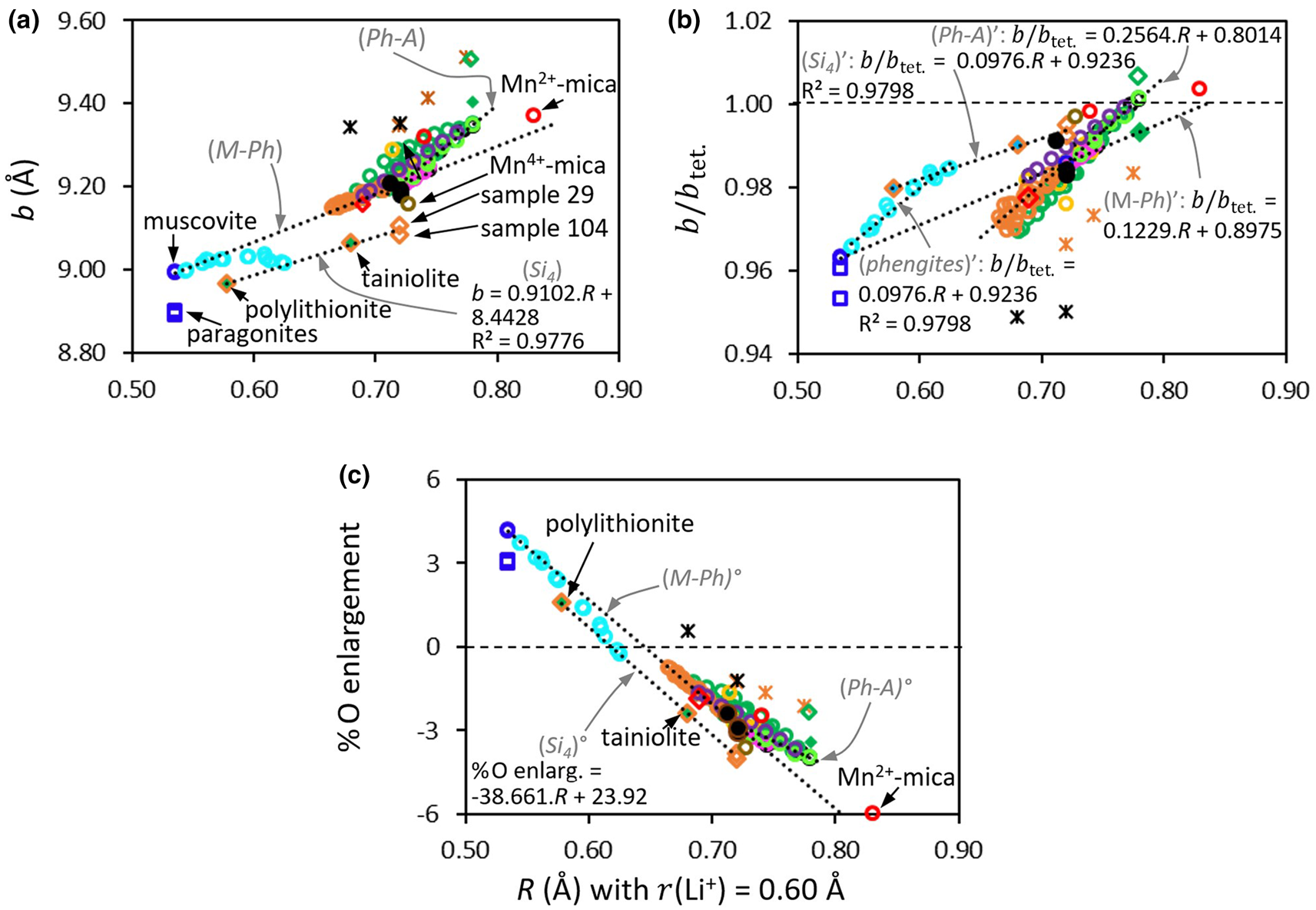
To assess the origins of the observed trends, we focus on synthetic micas because their chemical composition is less complex than that of natural systems and because chemical joins are available (Fig. 15a). The dataset of synthetic mica samples reveals generally similar trends to those of natural mica samples (Figs 12 & 14). The b/b tet. vs R plot for all of the synthetic samples reveals two main distinct but parallel trends for dioctahedral (muscovite–aluminoceladonite) and trioctahedral micas (phlogopite–annite; Fig. 15b). However, data for synthetic micas are lacking, especially for the compositional range corresponding to R ≈ 0.650. In natural micas, this compositional gap is filled by Li-micas and by celadonites and glauconites (Fig 12b & 14b).
Except for the Ni-mica, which is on the (M–Ph) and (M–Ph)’ lines, all of the trioctahedral trisilicic micas, including the rather ‘exotic’ Cu2+- and Co2+-micas (Hazen & Wones, Reference Hazen and Wones1972), are on or close to the (Ph–A) correlation line (Fig. 15a) and are also located near the (Ph–A)’ line due to their similar tetrahedral Al contents (Fig. 15b).
The synthetic Mn-mica approximately follows the muscovite–phlogopite trend in the b, b/b tet. and % O enlargement vs R plots (Fig. 15a–c). The % O enlargement is the smallest of all the dataset (–6% compared to hydroxides) and corresponds to the thickest O sheet very close to the dimensions of an unconstrained O sheet. Regarding the synthetic Fe2+ (annite) end member, b/b tet. is >1 (Fig. 15b). Unfortunately, the status of Mn is not sufficiently detailed (Frondel & Ito, Reference Frondel and Ito1966) to be confident regarding the greatest R and b tet. values. As Mn was assumed to be octahedral and divalent, some octahedral Mn3+ would have contributed to R, and thus the O sheet lateral dimensions would decrease, while tetrahedral Mn2+ would increase b tet. (Table 1).
Three synthetic mica series representing chemical joins will be studied in more detail below.
The first synthetic mica series corresponds to the dioctahedral mica series along the muscovite–aluminoceladonite join (K(Si3+xAl1–x)(Al2–xMgx)O10(OH)2 with x ≤ 1) of Schmidt et al. (Reference Schmidt, Dugnani and Artioli2001), which was also later studied and compared to natural samples by Zviagina & Drits (Reference Zviagina and Drits2019; Table 6). With increasing R, the dataset for these micas shifted away from the (M–Ph) line (Fig. 15a). Accordingly, Schmidt et al. (Reference Schmidt, Dugnani and Artioli2001) and Zviagina & Drits (Reference Zviagina and Drits2019) reported a ‘difficult to understand’ reduction of b for the greatest Mg content. Schmidt et al. (Reference Schmidt, Dugnani and Artioli2001) hypothesized that this reduction could be associated with a partial trioctahedral character, with some Mg possibly filling some M 1 octahedral sites (which are theoretically larger than the M 2 octahedra and are empty in ideally dioctahedral structures). Zviagina & Drits (Reference Zviagina and Drits2019) did not confirm this interpretation because their analysis of the M 1 octahedral site occupancies was negligible. Rather, these authors hypothesized that the change in the trend for b was associated with a decrease in mutual repulsion of octahedral cations with increasing contents of divalent cations, resulting in a reduced flattening of O sheets for the Mg-richest synthetic micas. This interpretation is confirmed by the % O enlargement vs R plot, where the data points deviate progressively from the (M–Ph)° line with increasing R (Fig. 15c). Moreover, the increase in octahedral charge related to the increase in the Al/Mg substitution rate in this sample series implies a concomitant decrease in tetrahedral charge to keep the layer charge at 1. The coupled increase in Mg and decrease in tetrahedral Al has a direct effect on the dimensional misfit reduction between the T and O sheets. A greater octahedral Mg content (and thus R), as hypothesized by Schmidt et al. (Reference Schmidt, Dugnani and Artioli2001), would not make b/b tet. decreases, as observed in Fig. 15b.
The second synthetic mica series corresponds to Al–Mg micas K(Si3–x+2yAl1+x–2y)(Mg3–x–yAlx□y)O10(OH)2 from the sample series of Robert (Reference Robert1976). These samples also lie on (or very close to) the (M–Ph) line, except sample 29 with the tetrasilicic composition Si4Mg2.5 (Fig. 15a). This sample series displays a wide range of compositions, with significant variation in the amounts of tetrahedral and octahedral Al as well as in octahedral Mg or vacant sites, whereas the octahedral occupancy ranges from 2.75 to 3, indicating a partial di-trioctahedral character. Robert (Reference Robert1976) observed a linear decrease in b with increasing octahedral Al content, but only for nine selected samples with a low number of vacant sites. As shown in Fig. 16a, b values for all of the di-trioctahedral Al–Mg micas (except sample 29) plotted as a function of R follow a linear regression, despite noticeable compositional changes in the T sheet composition, as IVAl contents range from 1 to 1.6 (Table 7). However, the regression coefficient is relatively low (R 2 = 0.95; Fig. 16a) and even decreases for the b/b tet. correlation (R 2 = 0.79; Fig. 16b), whereas it is very high for the % O enlargement (R 2 = 0.99; Fig. 16c). Several linear regressions can be observed between b and R depending on the parameter chosen (Table 7). For instance, if samples with the same y value in the SF are compared (i.e. samples having the same octahedral occupancy; Fig. 17a,b), then good correlations can be obtained using b or b/b tet. vs R graphs. As expected, the decrease in octahedral occupancy (increase in dioctahedral character) globally provokes a gradual decrease in the b dimension. For most y values, regressions with similar slopes can be drawn for at least the b/b tet. vs R graph (Fig. 17b & Table 7). Because this synthetic mica series can be described with x and y only, as seen in the general SF (i.e. Al, Mg, Si and vacant site amounts are interdependent), precise b or b/b tet. vs R graphs are also observed for each y = f(x) series (Figs 17c & 17d, respectively, & Table 7). As a consequence, the scattering of data that is greater in the b/b tet. vs R plot compared to the b vs R plot (Figs 16b & 16a, respectively) results from the superimposition of accurate sub-relationships. The general relationship b = 1.1509R + 8.3841 is likely to satisfactorily (± 0.006) predict b from R for this synthetic mica series (except sample 29) but corresponds to a general trend only. Sample 29 is a tetrasilicic mica and behaves differently from the other samples of the series. For the same R, it exhibits lower b and % O enlargement and greater b/b tet. (Fig. 16a–c) than the other samples. However, the synthetic tetrasilicic micas (i.e. the synthetic F counterpart of sample 29 (sample 108, tetrasilicic fluorophlogopite), polylithionite and tainiolite (with Li2Al and Mg2Li octahedral composition, respectively; Table 6; Brigatti & Guggenheim, Reference Brigatti, Guggenheim, Mottana, Sassi, Thompson and Guggenheim2002) follow trends that include sample 29 (Fig. 15a–c). The data points of the four samples are approximately aligned on a line that is approximately parallel to the muscovite–phlogopite line on all of the plots (Fig. 15a–c). Moreover, when adding the few natural tetrasilicic micas (i.e. some celadonites and a polylithionite (sample 45); Table 6; Rieder et al., Reference Rieder1970), a reasonably good regression is observed (Fig. 18a). Note that the samples of the muscovite–aluminoceladonite synthetic series of Schmidt et al. (Reference Schmidt, Dugnani and Artioli2001) presented above (K(Si3+xAl1–x)(Al2–xMgx)O10(OH)2) move to the tetrasilicic mica ‘(Si4)’ regression line and follow these trends when approaching a tetrasilicic composition (Fig. 15a–c). Even if the (Si4) regression cannot be considered as robust due to there being only few samples available and that the proposed revised r(Li+) of 0.6 Å used for calculating R for tainiolite and tetraferriphlogopite is only approximate, it argues indirectly for the suitability of r(Li+) ≈ 0.6 Å. Using the r(Li+) of 0.76 Å (Shannon, Reference Shannon1976) would lead to scattered data points (Fig. 18b).
Focus on the K(Si3–x+2yAl1+x–2y)(Mg3–x–yAlx□y)O10(OH)2 synthetic series of Robert (Reference Robert1976; Table 6). (a) b vs mean ionic radius of octahedral cations R. (b) b/b tet. vs R. (c) Percentage of octahedral enlargement vs R.

Focus on the K(Si3–x+2yAl1+x–2y)(Mg3–x–yAlx□y)O10(OH)2 synthetic series of Robert (Reference Robert1976; Table 6; sample 29 is not represented). (a) b vs R. (b) b/b tet. ratio vs R: dark blue: y = 0; light green: y = 0.025; red: y = 0.05; brown: y = 0.075; light blue: y = 0.1; pink: y = 0.125; yellow: y = 0.150; dark green: y = 0.175; orange: y = 0.225; open circles: single data point. Evolution of (c) b or (d) the b/b tet. ratio with the mean ionic radius of octahedral cations R: dark blue: y = 0; yellow: y = –0.5x + 0.25; green: y = –x + 0.5; red: y = –1.5x + 0,75; pink: y = –2x + 1; light blue: y = –2.5x + 1.25; brown: y = –3x + 1.5. See Table 7 for the corresponding regressions. (M–Ph) and (M–Ph)’ correspond to the muscovite–phlogopite regression lines.

b vs R for tetrasilicic K-micas (Table 6). (a) R calculated with r(Li+) = 0.6 Å. (b) R calculated with r(Li+) = 0.76 Å. Triangles = synthetic samples: pink = Mg2.5(OH)2-mica (sample 29; Robert, Reference Robert1976); red = Mg2.5F2-mica (sample 104; Brigatti & Guggenheim, Reference Brigatti, Guggenheim, Mottana, Sassi, Thompson and Guggenheim2002); green = Mg2Li-mica (tainiolite, sample 105; Brigatti & Guggenheim, Reference Brigatti, Guggenheim, Mottana, Sassi, Thompson and Guggenheim2002); orange = AlLi2–mica (polylithionite). Circles = natural samples: orange = polylithionite (sample 45; Rieder, Reference Rieder1970); blue = celadonites; brown = norrishite ((LiMn3+2)-mica, sample 111; Brigatti & Guggenheim, Reference Brigatti, Guggenheim, Mottana, Sassi, Thompson and Guggenheim2002). Symbols filled in green = Li-containing micas.

Note that norrishite (KSi4(LiMn3+2)-mica, sample 111; Table 6; Brigatti & Guggenheim, Reference Brigatti, Guggenheim, Mottana, Sassi, Thompson and Guggenheim2002) is systematically outside of all of the trends (Figs 12–14 & 18). Accordingly, Brigatti & Guggenheim (Reference Brigatti, Guggenheim, Mottana, Sassi, Thompson and Guggenheim2002) also observed an anomalous behaviour of this norrishite sample compared to the other micas, which they related to octahedral distortions induced by the Jahn–Teller effect.
In conclusion, the impact of R on b is similar between tetrasilicic and trisilicic micas, and the lower b observed for tetrasilicic micas is related to a reduced flattening of O sheets compared to in trisilicic micas.
The third and last synthetic mica series that will be studied corresponds to the trioctahedral micas (Si3–zAl1+z)(MgxFe2+yAlz)K (Hewitt & Wones, Reference Hewitt and Wones1975; Redhammer & Roth, Reference Redhammer and Roth2002; Mercier et al., Reference Mercier, Rancourt, Jean-Louis, Berman and Redhammer2005) that appear slightly above the (Ph–A) and (M–Ph) lines in the b vs R and % O enlargement vs R plots (Figs 15a & 15c, respectively) and on or below the (Ph–A)’ line in the b/b tet. vs R plot (Fig. 15b). A reduced scattering of data is noticed in the b/b tet. vs R plot, as illustrated by the respective regression coefficients (calculated using the Hewitt & Wones, (Reference Hewitt and Wones1975) series only, R 2 = 0.82, 0.97 and 0.89; Figs 19a, 19b & 19c, respectively). As for the previous synthetic mica series, several sub-relationships can be noticed that correspond to specific solid solutions. As an illustration, for constant values of z (Al content), linear regressions corresponding to the respective Mg–Fe2+ solid solutions are observed (Fig. 20a). In such solid solutions, b systematically decreases with the Fe2+:Mg ratio, as expected considering the respective ionic radii of Mg and Fe2+ (Table 1). The slopes of these regression lines increase slightly from ~2.4 to 2.9 with increasing z (Table 7). For z = 0, the equation is very similar to that of the (Ph–A) line. The small difference is assigned to the fact that both regressions were calculated in different ways, using the end member data for the (Ph–A) regression and using the solid solution for z = 0. The slopes for each Mg–Fe2+ solid solution linear regression are more than twice as high as those for (Si3–zAl1+z)(Mg3–zAlz)K and (Si3–zAl1+z)(Fe2+3–zAlz)K, which exhibit similar slopes to each other (Table 7). The regression for the (Si3–zAl1+z)(Mg3–zAlz)K solid solution is close to that of the (M–Ph) line, and the small difference is due to the strictly trioctahedral character due to by Tschermak substitutions in the sample series of Hewitt & Wones (Reference Hewitt and Wones1975) compared to the di-trioctahedral muscovite–phlogopite solid solution. The b/b tet. vs R plot reveals that regressions also exist for each solid solution (Fig. 20b). The misfit between T and O sheets increases with decreasing R (i.e. with decreasing amounts of Fe2+ relative to Mg) and more severely with increasing Al content due to Tschermak substitutions and the antagonistic effect of Al, as discussed above for Al-serpentines. For the trisilicic Fe2+ end member, b/b tet. slightly exceeds 1 (Fig. 20b), suggesting a T sheet that is fully extended with a symmetry close to hexagonal to fit the large lateral O sheet dimension. Accordingly, the O sheet is the thickest of the series (Fig. 20c).
Focus on the K(Si3–zAl1+z)(MgxFe2+yAlz)O10(OH)2 synthetic series. Black circles from Hewitt & Wones (Reference Hewitt and Wones1975), green crosses from Redhammer & Roth (Reference Redhammer and Roth2002), blue crosses from Mercier et al. (Reference Mercier, Rancourt, Jean-Louis, Berman and Redhammer2005; Table 6). (a) b vs mean ionic radius of octahedral cations R. (b) b/b tet. vs R. (c) Percentage of octahedral enlargement vs R. The dashed lines correspond to muscovite–phlogopite (M–Ph) and phlogopite–annite (Ph–A) regression lines. The dotted line is the regression calculated using the Hewitt & Wones (Reference Hewitt and Wones1975) data.

Focus on the K(Si3–zAl1+z)(MgxFe2+yAlz)O10(OH)2 synthetic series of Hewitt & Wones (Reference Hewitt and Wones1975; Table 6). Evolutions of (a) b, (b) b/b tet. ratio and (c) percentage of octahedral enlargement with the mean ionic radius of octahedral cations R for green circles: z = 0; blue circles: z = 0.25; yellow circles: z = 0.50; grey circles: z = 0.63; pink circles: z = 0.75; pink open square: calculated by extrapolation; red circles: single data point with the indicated z value. Dotted lines = linear regression for each z series (see Table 7 for the corresponding regressions). The dashed lines correspond to muscovite–phlogopite (M–Ph) and phlogopite–annite (Ph–A) regression lines.
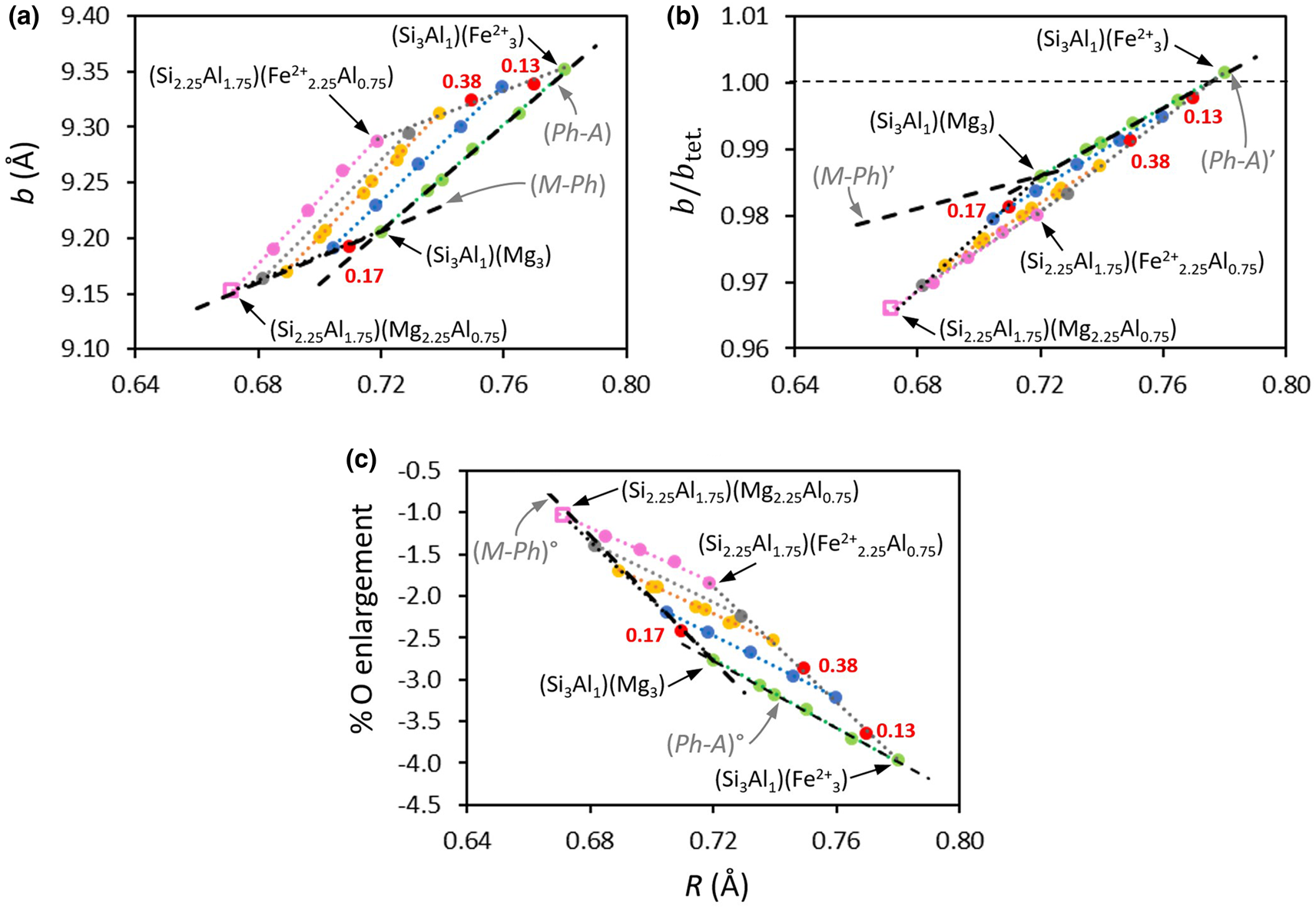
The increase of tetrahedral Al content induces an increase in lateral T sheet dimensions and the thinning of O sheets via octahedral flattening to reduce the misfit (Fig. 20c). For the same Al content, the octahedral flattening also increases with increasing Mg/Fe2+ substitution, contributing to the tetrahedral rotation to reduce the misfit. The cumulative effect is demonstrated here by the increase in the slope of the regressions with increasing Al content (i.e. increasing z; Fig. 20 & Table 7). As for the sample series of Robert (Reference Robert1976), the scattering of data observed for the series of Hewitt & Wones (Reference Hewitt and Wones1975) is assigned to the superimposition of accurate sub-relationships corresponding to limited solid solutions.
In light of the results obtained for synthetic micas, the observed scattering of data (Figs 12 & 14) for all of the datasets is mainly due to the chemical complexity of the samples, and multiple limited solid solutions probably exist between a multitude of end members.
Chlorites
Chlorites are phyllosilicates composed of 2:1 layers whose negative charge, arising mainly from heterovalent tetrahedral substitutions, is most often balanced by the presence of a positively charged O sheet in the interlayer space (Fig. 1a; e.g. Bailey, Reference Bailey and Bailey1991a). The structure of chlorite is then globally electrostatically neutral, with a general SF of (Si4–xAlx)(R 3+yR 2+z□v)O10(OH)8, where □ is a vacant site and y + z + v = 6. The composition of the layer is (Si4–xAlx)(R3+R 2+□)3O10(OH)2 and that of the interlayer octahedral sheet is (R 3+R 2+□)3(OH)6. It is difficult to determine the composition of each of them accurately (e.g. Zazzi et al., Reference Zazzi, Hirsch, Leonova, Kaikkonen, Grins, Annersten and Eden2006), especially because the chemical composition of chlorites is very variable (e.g. see the review of Wiewiora & Weiss, Reference Wiewiora and Weiss1990). Trioctahedral chlorites (trioctahedral in both the layer and the interlayer) are the most common in nature, and several families exist, such as clinochlore, chamosite and penninite, with Mg, Fe2+ and Mn2+ as the dominant octahedral cations, respectively.
Due to the complex chemical composition of chlorite, numerous studies have been devoted to the relations between b and the amounts of octahedral and tetrahedral cations. Several equations with the form of $b = b_0 + \mathop \sum \nolimits_{i = 1}^n ( {a_ix_i} )$ can be found in the literature (von Engelhardt, Reference von Engelhardt1942; Radoslovich Reference Radoslovich1962), especially for trioctahedral chlorites, as exemplified by Lee et al. (Reference Lee, Guggenheim, Dyar and Guidotti2007), who observed a robust linear relationship between b and Mg/Mg + Fe for natural chlorite samples from Al-saturated metamorphic assemblages. Wiewiora & Wilamowski (Reference Wiewiora and Wilamowski1996) formulated two distinct regression equations for trioctahedral chlorites (Equation 7) and di-tri- and di-dioctahedral chlorites (Equation 8) as follows:


The dataset used in the present study is taken mainly from the review work of Wiewiora & Wilamowski (Reference Wiewiora and Wilamowski1996), where several b values were measured using structural refinement. To avoid any potential bias from using a unique data source and to enlarge the range of chemical compositions investigated for chlorite, the compiled data from Radoslovich (Reference Radoslovich1962) were added, as well as a few other samples (i.e. two samples whose single-crystal structure has been refined: one ordered triclinic clinochlore (Smyth et al., Reference Smyth, Dyar, May, Bricker and Acler1997) and one cookeite (Zheng & Bailey, Reference Zheng and Bailey1997b); and four uncommon chlorites, namely V3+-rich chlorites (Whitney & Northrop, Reference Whitney and Northrop1986) and Fe3+-sudoites (Billault et al., Reference Billault, Beaufort, Patrier and Petit2002; Table 8).
Data used for chlorites.

b is a crystallographic parameter (Å).
R = mean ionic radius of octahedral cations (Å) calculated with r(Li+) = 0.76 Å (see text for details).
a Sample reference in the paper.
b Typographical error; original value: Al0.85Mg0.7Fe2+0.75Fe3+3.7.
c Instead of Mg4.175 – corrected from the source paper (Zheng & Bailey, Reference Zheng and Bailey1989).
The evolution of b as a function of R for all samples reveals reasonably good data alignment for all compositions ranging from dioctahedral to trioctahedral chlorites (Fig. 21a). In contrast to Wiewiora & Wilamowski (Reference Wiewiora and Wilamowski1996), the b vs R regression is suitable for the entire range of chemical compositions. R values for di-tri- and trioctahedral chlorites even overlap in the intermediary range (for 0.64 < R < 0.70). This is probably because trioctahedral occupancy with cations of various valences, such as (R 3+xR 2+3–x) and (R 3+xR +3–x), is expected to occur in chlorites, at least in the interlayer O sheets, to counterbalance the negative tetrahedral charge. The clinochlore and cookeite samples with refined single crystals fall on or close to the correlation line. The uncommon vanadium-rich chlorites (Whitney & Northrop, Reference Whitney and Northrop1986), assuming Fe and V as trivalent cations, as well as Fe3+-sudoites (Billault et al., Reference Billault, Beaufort, Patrier and Petit2002), do not reveal any specific behaviour (Fig. 21a). Some samples, such as samples 8, 28 and 30 (Table 8), deviate significantly from the regression line (Fig. 21a). For sample 28, R is suspected to be underestimated due to a redox problem, as the Fe2+:Fe3+ ratio was reversed in a previous study (Steinfink, Reference Steinfink1958). As sample 8 was classified in the trioctahedral group, the Fe2+ and Fe3+ contents have probably been switched mistakenly (Table 8), and the data point moved close to the regression line after switching back both contents (Fig. 21a). Other typographical errors cannot be excluded, as another one could be identified for sample 82 (Table 8). Unfortunately, data for sample 30 are unpublished and could not be checked.
b vs R for chlorites (Table 8). Calculation of R performed with (a) r(Li+) = 0.76 Å and (b) r(Li+) = 0.60 Å. Dark blue circles = di-tri and di-dioctahedral chlorites; yellow circles = trioctahedral chlorites; dark green circles = various chlorites (Radoslovich, Reference Radoslovich1962); pink circles = vanadium chlorites; light green circles = Fe3+-sudoites; red circle = clinochlore (Smyth et al., Reference Smyth, Dyar, May, Bricker and Acler1997); light blue circle = cookeite (Zheng & Bailey, Reference Zheng and Bailey1997b); open circles = Li-containing chlorites; dotted line = regression calculated with all samples.

Some chlorites of the di-tri- and di-di-octahedral series are Li-rich. The Al2Li configuration is likely to occur in the interlayer hydroxide sheet to create a positive charge balancing the tetrahedral negative charge (Zheng & Bailey, Reference Zheng and Bailey1997b). The revised r(Li+) of 0.60 Å (instead of 0.76 Å) determined for Li-rich micas (see above) was used as an alternative (Fig. 21b). The general regression was modified slightly to b = 2.30R + 7.67, and the regression coefficient was improved slightly (R 2 = 0.865 vs 0.884), arguing for the suitability of a lower r(Li+).
Contrary to Wiewiora & Wilamowski (Reference Wiewiora and Wilamowski1996), who included tetrahedral Al in their equations with a greater coefficient for di-tri- and di-dioctahedral chlorites than for trioctahedral chlorites (Equations 7 & 8), the unique linear regression (Fig. 21b) indicates that b is mainly driven by R and that the tetrahedral Al is not a first-order parameter. Accordingly, a unique main trend is also observed for the b/b tet. vs R regression, although its coefficient is lower than for the b vs R regression (0.78 (Fig. 22a) and 0.88 (Fig. 21b), respectively). The observed dispersion of data points may be partly due to the scattering of tetrahedral charge ranging from 0.45 to 1.80 (Table 8), but we cannot confident in their accuracy for the entire dataset.
(a) b/b tet. and (b) percentage of octahedral enlargement vs R calculated with r(Li+) = 0.60 Å for chlorites (Table 8). Same samples and colour code as in Fig. 21. (c) Tetrahedral rotation angle measured using structural refinement αref vs calculated tetrahedral rotation angle αcalc: blue = using fixed Si–O and Al–O bond lengths (1.618 and 1.748 Å, respectively); orange = using mean T–O bond lengths obtained using structural refinement (see Table 9 and text for details). The dashed line represents the line of isovalues.

Summary of tetrahedral parameters of chlorite. Sample reference from Table 8. Tetrahedral rotation angle αref: measured using structural refinement; αcalc: calculated (α = arccos(b/b tet.); Equation 4; see text for details).

a Sample reference in the paper.
b From structural refinement.
c Calculated using the following equation derived from Equation 3: (Si–O) = (b tet. – √2IVAlΔ)/(4√2), with b tet. obtained from Equation 4 along with αref, and with Δ = 0.13 being the difference between Si–O and Al–O bond lengths.
The b/b tet. values vary from 0.952 (dioctahedral chlorites) to 1.009 (trioctahedral chlorites), which correspond to angles of tetrahedral rotation α ≈ 18° and 0°, respectively, matching relatively well with α measured using structural refinement: ~14° for dioctahedral donbassite and ~5–7° for trioctahedral chlorites (Bailey, Reference Bailey and Bailey1991a). Focusing on some samples whose single-crystal structure was refined (Table 9), an excellent relationship is observed between αref (the tetrahedral rotation angle measured using structural refinement) and αcalc (the tetrahedral rotation angle calculated from b/b tet.; Equation 4; Fig. 22c). Surprisingly, the regression coefficient is greater when using Si–O and Al–O bond lengths of 1.618 and 1.748 Å, respectively, following Bailey (Reference Bailey and Bailey1984a), than when using the T–O mean bond length determined using structural refinement (Fig. 22b). The Si–O and Al–O bond lengths were calculated to match αref, and very coherent values were obtained (Table 9). This study also shows that by using adequate bond lengths, Equation 4 allows us to calculate the angle of tetrahedral rotation α accurately, at least for most of the common samples.
Going from dioctahedral chlorites to trioctahedral ones (i.e. with R increasing), the tetrahedral rotation angle α progressively decreases, as shown by the b/b tet. plot (Fig. 22a), while the flattening of O sheets decreases concomitantly (Fig. 22b). For di- and di-tri-octahedral chlorites, O sheets are thinner than the hydroxides with the same R, whereas they are thicker for trioctahedral chlorites.
In chlorite, the element partitioning between both O sheets will not affect R significantly, which is a mean value, but such a partitioning is likely to impact the misfit between the T and O sheets. As for the other phyllosilicate families, the misfit between T and O sheets increases when R decreases, and both shortening of T sheets by tetrahedral rotation and flattening of O sheets are expected to occur. Most trioctahedral chlorites show b/b tet. values close to 1, demonstrating the easy accommodation of the T and O sheets. Samples with the greatest b/b tet. and R values are Mn-rich and have a great tetrahedral Al content (cf. samples 1, 2 and 3 of the trioctahedral series of Wiewiora & Wilamowski (Reference Wiewiora and Wilamowski1996) and sample ‘pennantite’ of Radoslovich (Reference Radoslovich1962); Table 8). For these samples, both the T and O sheets have large lateral dimensions, and misfit compensation is likely to be facilitated. It is worth noting that the clinochlore and cookeite samples with refined single crystals fall very close to the b, b/b tet. and % O enlargement vs R plot correlation lines (Figs 21 & 22). In this regard, the data scattering shown in Fig. 21 is probably related to the structural complexity of chlorites associated with multiple possibilities of misfit accommodation, variable composition and charge balance between T and O sheets and chemical uncertainties.
Discussion
For the samples studied (i.e. hydroxides, oxyhydroxides, LDHs, TO phyllosilicates (kaolinite–lizardite or modulated series), neutral TOT phyllosilicates (pyrophyllite–talc series), smectites (same as the neutral TOT phyllosilicates), micas (muscovite–phlogopite, phlogopite–annite, tetrasilicic micas series) and chlorites), the first-order relation in Equation 10 can be applied:

The A and B parameters for the various families are reported in Table 10. The ionic radii dataset taken from Shannon (Reference Shannon1976) allows us to obtain suitable R values, except for Mn3+, as discussed for groutite, and Li+, as discussed for micas and chlorites, for which a smaller size appears to be more suitable. The equations for the regressions of these minerals were reported (Table 10) with R calculated with r(Li+) = 0.60 Å rather than the 0.76 Å value from Shannon (Reference Shannon1976).
Regression parameters proposed for the various mineral families investigated.

a Compared to hydroxides.
b See Table 7 for details on sub-relationships.
c Refers to phengites.
d Refers to micaceous samples.
The b vs R correlation lines determined for all of the studied mineral families were reported on the same plot (Fig. 23a). Note that the development of correlation lines does not necessarily imply the existence of a complete isomorphous series between end members, which is obviously dependent on their physicochemical conditions of formation and thermodynamic stability. Samples that are not represented on this plot because no b vs R linear relation could be observed will be discussed later. b of a calculated theoretical ‘free’ T Si–O sheet (= b tet.) is ~9.15 Å and increases with tetrahedral substitution (Equation 3; b tet. ≈ 9.34 Å for Si0.75IVAl0.25). The determined b vs R regression for Mn +(OH)n hydroxide structures can be considered as representing the ‘free’ O sheets (i.e. without any constraint from the T sheets). The T sheet and O sheet (hydroxides) lines intercept at R ≈ 0.65 Å and at R ≈ 0.69 Å when a quarter of Si is substituted by Al (Fig. 23a).
(a) b vs R calculated with r(Li+) = 0.60 Å for the various studied phyllosilicates structures: horizontal dashed grey lines = calculated theoretical ‘free’ T sheet (dark grey: unsubstituted; light grey: Si0.75IVAl0.25); black dashed line = experimentally determined regression for hydroxides (see text for details); coloured dotted lines = regression lines determined in this study, such as kaolinite–lizardite (K–L), pyrophyllite–talc (P–T), muscovite–phlogopite (M–Ph), phlogopite–annite (Ph–A), tetrasilicic micas (Si4), (chlorites) and TO-modulated phyllosilicates (G–C). (b) b/b tet. vs R for the same phyllosilicates as in (a). (c) Percentage of octahedral enlargement compared to hydroxides (see text for details) vs R for the same phyllosilicates as in (a). The intersections between the 0% O enlargement line (black dashed line) and the coloured dotted lines correspond to R for which the thickness of the O sheets is the same for phyllosilicates and hydroxides. Above this 0% O enlargement line, the O sheets of phyllosilicates are thinner than the hydroxides for the same R, whereas below this line they are thicker.

The slope of the regression line (i.e. the A parameter in Equation 10) is found to be significantly higher for hydroxides than for phyllosilicates, except for the TO phyllosilicates with modulated structures (Fig. 23a & Table 10). Such a contrast demonstrates the prominent role played on b by the misfit accommodation between the lateral dimensions of the O and T sheets. This finding was used to derive a structurally based interpretation of the evolution of b with R in terms of processes of misfit accommodation.
Globally, at the lattice scale, the b vs R linear relations (Fig. 23a) were interpreted mainly as resulting from the misfit accommodation by coupling more or less pronounced tetrahedral rotation and O sheet flattening whatever the value of R. These two processes are often presented as being the main ways by which to accommodate misfit in micas (e.g. Radoslovich, Reference Radoslovich1962; Donnay et al., Reference Donnay, Morimoto, Takeda and Donnay1964; Toraya, Reference Toraya1981). From dioctahedral to trioctahedral phyllosilicates, a decrease of the tetrahedral rotation angle α allows us to decrease the lateral T sheet dimension, whereas a thickening of the O sheet allows us to decrease the lateral O sheet dimension. The b/b tet. and % O enlargement vs R plots (Figs 23b & 23c, respectively) are complementary representations of the b vs R plot (Fig. 23a), allowing us to distinguish better the respective roles of the T and O sheets.
For TO phyllosilicates (excluding IVAl- and IVFe3+-serpentines and modulated phyllosilicates), TOT neutral structures, micas (excluding those with small interlayer cations (Na and Ca) and with interlayer depletion (micaceous samples)) and chlorites, the O sheet dimension, and thus R, mainly drives b. The various slopes observed (Fig. 23a) for the various families are then related to the relative importance of the adjustments of T and O sheets in the misfit accommodation. This agrees well with Bailey (Reference Bailey and Bailey1984b), who stated that ‘the T sheets appear sufficiently flexible to conform to the lateral dimensions dictated by smaller O sheets, and T and O lateral dimensions are similar enough that articulation of T with O sheets can be accomplished readily by tetrahedral rotation and additional thinning or thickening of O sheets’. The thinning or thickening of phyllosilicate O sheets is compared here to the thickness of their hydroxide counterparts (i.e. hydroxides with the same R as the considered phyllosilicates).
It is worth noting that O sheet thickening occurs (% O enlargement < 0 in Fig. 23c) when the O sheet remains smaller than the T sheet (b/b tet. < 1 in Fig. 23b).
For tetrasilicic micas and the muscovite–phlogopite mica series, b < b tet.. whatever the value of R (Fig. 23b), whereas the octahedral flattening varies continuously, with the thicknesses of O sheets being similar to those of their hydroxide counterparts for R ≈ 0.62 and 0.65 Å, respectively (Fig. 23c). The slopes of the tetrasilicic mica (Si4)° and trisilicic mica (M–Ph)° regression lines are similar. For the same R, b values and flattening of the O sheet are greater for trisilicic micas than for tetrasilicic micas (Fig. 23c), agreeing well with the O sheet thickness measured using structural refinement (Table 11). Only one refined data point for talc was available for comparison with neutral TOT structures without interlayer cations, as the (P–T)° line also has a similar slope to the tetrasilicic (Si4)° and trisilicic (M–Ph)° mica lines.
Structural details for some phyllosilicates for comparison. Sample reference from Table 6 for micas and Table 4 for talc. R calculated using r(Li+) = 0.60 Å. Tetrahedral rotation angle αref: measured using structural refinement; αcalc: calculated (α = arccos(b/b tet.); Equation 4; see text for details). % O enlargement compared to hydroxides; O sheet thickness measured by structure refinement and αref: from Brigatti & Guggenheim (Reference Brigatti, Guggenheim, Mottana, Sassi, Thompson and Guggenheim2002) for micas and from Drits et al. (Reference Drits, Guggenheim, Zviagina and Kogure2012) for talc.

For talc, the octahedral flattening is comparatively more pronounced than for tetrasilicic micas and comparatively less pronounced than for trisilicic micas (Fig. 23c), agreeing well with the O sheet thicknesses (Table 11). However, the calculated values of the tetrahedral rotation angle α are lower for tetrasilicic micas compared to trisilicic ones, but they are far greater than the measured ones (Table 11). For tetrasilicic micas, the tetrahedral rotations probably have to be limited to ensure sufficiently large holes for K, and the contribution of the O sheet has to be more pronounced to allow congruency between the O and T sheet dimensions.
For lizardites and talcs, b > b tet. for R > ~0.67 and ~0.70 Å, respectively (Fig. 23a), but for the tetrasilicic and muscovite–phlogopite micas, the octahedral flattening varies continuously whatever the value of R.
For chlorites and phlogopite–annite, the O sheet becomes greater in the lateral dimension than T sheet for high R, and tetrahedral substitution rates are greater and thickening of O sheets occurs more strongly than for the other phyllosilicates (Fig. 23c).
These results agree well with previous works (e.g. Toraya, Reference Toraya1981; Lin & Guggenheim, Reference Lin and Guggenheim1983; Weiss et al., Reference Weiss, Rieder, Chmielová and Krajíček1985, Reference Weiss, Rieder and Chmielová1992), and especially with Hazen & Wones (Reference Hazen and Wones1972), who suggested that octahedral flattening is controlled by the octahedral cation radius.
The aforementioned structurally based interpretation probably underlies the approximately similar regression lines observed for the (K–L), (P–T), (Si4) and (M–Ph) sample series (Fig. 23a), suggested that tetrahedral rotations and O sheet flattening are the primary crystallographic distortions allowing the T and O sheet accommodation. The role of the presence of a T sheet on b can also be evidenced by analysing the evolution of the b vs R regression line of trioctahedral micas and chlorites. The greater b values obtained for these minerals for great R values compared to other phyllosilicates (Fig. 23a & Table 10) could be due to the presence of trioctahedral O sheets coupled to large lateral T sheet dimensions. The above two features probably strengthen the decrease in tetrahedral rotation (Fig. 23b) and limit O sheet flattening (Fig. 23c) in trioctahedral micas and chlorites compared to the other phyllosilicates.
The (G–C) line exhibits a greater slope than the correlation obtained for chlorites or even for the hydroxides (Fig. 23a). This probably indicates a strong influence of the O sheets (which are similar to hydroxides sheets; Fig. 6b) over the T sheets for the (G–C) sample series and may explain the origins of the observed corrugated structures as a way to accommodate the dimensional misfit in these minerals. Such a mechanism is less likely to occur for TOT structures due to the constraints applied by the two sandwiching T sheets. The (G–C) line intersects the correlation line for chlorites when the dimensional misfit between T and O sheets is minimal (Fig. 23a). Note that even if the slope of the (G–C) line is greater than that observed for the hydroxides, the two lines never intersect (Fig. 23a), probably providing evidence of a structural limit to misfit accommodation.
The similarity of b values between chlorites and serpentines for the same octahedral composition may explain their intimate relationships in geological processes (e.g. Ryan & Hillier, Reference Ryan and Hillier2002; Zhang et al., Reference Zhang, Gilbert and Banfield2021).
For IVAl- and Fe3+-serpentines, excellent regressions were obtained for b/b tet. vs R (Fig. 6a), and the results obtained using Equation 10 were improved by integrating the tetrahedral sheet composition using Equation 11:

with b tet. calculated according to Equation 3 and C and D being experimentally obtained regression parameters (Table 10).
As expected, micas with small interlayer cations (Na and Ca) or those that are not silicic appear ouside of the trends, and specific processes that ensure congruency between sheets cannot be assessed using this simplistic approach.
The schematized, structurally based interpretation of the control of b by R in hydroxides and various phyllosilicates represents the principal processes but is not unique. As evidenced for the synthetic mica series, the presence of sub-relationships related to limited solid solutions is also responsible for variations in the regression lines. Moreover, this study shows that for smectites and micas, as expected, the layer charge, especially that arising from tetrahedral substitution, probably also impacts the observed b values.
Conclusion
According to the abundant literature, the octahedral chemical composition of phyllosilicates is related to b. Using the mean ionic radius of octahedral cations, R allows us to generalize the various correlations that can be found in the literature between b and the octahedral chemistry of phyllosilicates and hydroxides, which are often restricted to limited types of sample series in terms of chemical composition or dioctahedral vs trioctahedral character. Integrating the tetrahedral sheet composition using b tet. for phyllosilicates that possess tetrahedral substitutions improves the relation between b and R.
A nanomechanistic interpretation based on misfit accommodation by coupling more or less pronounced tetrahedral rotation and O sheet flattening explains the results well globally, and this potentially impacts the processes of formation and transformation of phyllosilicates.
Refining the proposed model to account for structural peculiarities could represent a logical next step to this work.
Acknowledgements
We thank the anonymous reviewers for their careful and constructive reviews, which improved the quality of the paper significantly. We also thank Milan Rieder, who kindly provided us with a valuable table of mica data he obtained half a century ago, and Alain Meunier for his valuable comments on a preliminary version.
Financial support
We thank the European Joint Program EURAD (WP ‘Future’ – grant ID 847593), the French government programme ‘Investissements d'Avenir’ (EUR INTREE, reference ANR-18-EURE-0010) and the European Union (ERDF) and ‘Région Nouvelle Aquitaine’ for providing financial support for this study.
Conflicts of interest
The authors declare none.


 Open access