


Impact statement
Floating marine litter is a worldwide emerging problem that threatens marine ecosystems. Monitoring distribution and fate of Floating Macro Marine Litter (FMML) is becoming a pressing need to support mitigation strategies. Recently, the use of detection technologies based on satellite images is a promising approach for FMML monitoring with large spatial coverage and acceptable time resolution. In this study, we tested a scalable and transferable machine learning detection framework for FMML. We applied this approach to a long-time series satellite images of the Pearl River Estuary, one of the world largest coastal urbanized area. The MARIne Debris Archive trained classifier applied to Sentinel-2 imagery enables a detailed analysis of the spatial and temporal distribution patterns of FMML. These findings are useful in understanding marine debris transport mechanics also at different scales. Locally, these results could raise awareness of marine debris problem in the PRE and Hong Kong Waters due to rapid economic development that leads to increased plastic pollution. Regionally, the study improves our understanding of marine debris transport pathways and accumulation hotspots, providing insights that might guide environmental management strategies in the South China Sea and beyond. Globally, the study can be replicated in other coastal regions around the world, contributing to the global effort to reduce marine pollution in the view of Sustainable Development Goal 14. Our research also illustrates the potential of satellite-based monitoring as an efficient tool for large-scale environmental assessments that overcomes the limitations of traditional methods such as manta trawling and visual observations. The integration of hydrodynamic data with remote sensing increases the accuracy and reliability of marine debris detection. This work provides the foundation for informed decision-making and policy development. Our research not only advances scientific knowledge but also provides practical solutions for one of the most urgent environmental challenges of our time.
Introduction
Marine Debris (MD) comprises a wide range of anthropogenic materials, such as plastics, rubber, and organic debris, which enter the marine environment via various pathways (Voronkova et al., Reference Voronkova, Richter, Henderson, Aruta, Dumbili, Wyles and Pahl2023; Secretariat, Reference Secretariat2025). One of the main causes of the MD problem is the rapid increase in plastic production and use, which is driven by urban expansion, economic development (Geyer et al., Reference Geyer, Jambeck and Law2017; Lebreton and Andrady, Reference Lebreton and Andrady2019; Jahandari, Reference Jahandari2023; Brglez et al., Reference Brglez, Čuček, Krajnc and Lukman2024). Global plastic production has surged from 2 million tons in 1950 to 460 million tons in 2023, greatly exceeding the global recycling rate of just 9%, while most of the unrecycled plastic has leaked into the aquatic environment (Lebreton et al., Reference Lebreton, Slat, Ferrari, Sainte-Rose, Aitken, Marthouse, Hajbane, Cunsolo, Schwarz, Levivier, Noble, Debeljak, Maral, Schoeneich-Argent, Brambini and Reisser2018; Borrelle et al., Reference Borrelle, Ringma, Law, Monnahan, Lebreton, McGivern, Murphy, Jambeck, Leonard, Hilleary, Eriksen, Possingham, De Frond, Gerber, Polidoro, Tahir, Bernard, Mallos, Barnes and Rochman2020; OECD, 2022; Sojobi and Zayed, Reference Sojobi and Zayed2022; Waqas et al., Reference Waqas, Wong, Stocchino, Abbas, Hafeez and Zhu2023; Europe, Reference Europe2025). Due to plastic’s natural resistance to degradation (plastic mineralization may take up to 1,400 years to be completed), the amount of MD in water bodies is rising steadily (Chamas et al., Reference Chamas, Moon, Zheng, Qiu, Tabassum, Jang, Abu-Omar, Scott and Suh2020). The Great Pacific Garbage Patch (GPGP) is a prime example of global MD mismanagement. It has been found that it covered an area of 1.6 million square kilometers in 2018, with an approximate weight of 79,000 tons (Lebreton et al., Reference Lebreton, Slat, Ferrari, Sainte-Rose, Aitken, Marthouse, Hajbane, Cunsolo, Schwarz, Levivier, Noble, Debeljak, Maral, Schoeneich-Argent, Brambini and Reisser2018; Egger et al., Reference Egger, Sulu-Gambari and Lebreton2020; Kunz et al., Reference Kunz, Griesel, Eden, Duran and Sainte-Rose2024; Lebreton et al., Reference Lebreton, De Vries, Pham, Wolter, Van Vulpen, Puskic, Sainte-Rose, Royer and Egger2024). Some of the retrieved MDs are originated from the 1970s, hinting at the persistent deposition of marine litter (Lebreton et al., Reference Lebreton, Slat, Ferrari, Sainte-Rose, Aitken, Marthouse, Hajbane, Cunsolo, Schwarz, Levivier, Noble, Debeljak, Maral, Schoeneich-Argent, Brambini and Reisser2018).
Furthermore, the rotating gyre hydrodynamics features of GPGP also make it a perfect transport vector for invasive species, while releasing harmful chemicals, such as pesticides (De-La-Torre et al., Reference De-La-Torre, Arribasplata, VaL, Póvoa and Walker2023; Mghili et al., Reference Mghili, De-La-Torre and Aksissou2023; Ouyang et al., Reference Ouyang, Panti, Canicci, Li and Tam2023). In the meantime, under the effects of hydrodynamic forcing (e.g., sea wave actions), the larger MD has been observed to fragment into smaller pieces, enter the biomass, and inevitably threaten biodiversity, for example, reef-building corals (Gall and Thompson, Reference Gall and Thompson2015; Vethaak and Legler, Reference Vethaak and Legler2021; Yee et al., Reference Yee, Hii, Looi, Lim, Wong, Kok, Tan, Wong and Leong2021; Andrady, Reference Andrady2022; Nihart et al., Reference Nihart, Garcia, Hayek, Liu, Olewine, Kingston, Castillo, Gullapalli, Howard, Bleske, Scott, Gonzalez-Estrella, Gross, Spilde, Adolphi, Gallego, Jarrell, Dvorscak, Zuluaga-Ruiz and Campen2025).
In view of the projected doubling or even tripling of MD by the year 2040, the United Nations classifies the MD problem as one of the emerging threats within SDG14. Despite the fact that strategic mitigation frameworks have been established, effective monitoring networks for source identification are lacking, and needs are prioritized (UNEP, 2025). Traditional MD monitoring and surveying techniques, such as manta trawling, visual observations, and beach clean-ups, are generally demanding in terms of resources and require a special care during the collection stage and laboratory analysis (Cutroneo et al., Reference Cutroneo, Reboa, Besio, Borgogno, Canesi, Canuto, Dara, Enrile, Forioso, Greco, Lenoble, Malatesta, Mounier, Petrillo, Rovetta, Stocchino, Tesan, Vagge and Capello2020). More importantly, the spatial coverage of traditional methods can be limited, indicating that it may be insufficient in capturing the MD dynamics on a large scale, especially in dynamic aquatic environments (Maximenko et al., Reference Maximenko, Hafner, Kamachi and MacFadyen2018; GESAMP, Reference GESAMP2019). However, effective MD management does require an understanding of the spatial–temporal dynamics of MD, such as distributions, transport patterns, and accumulation hotspots in a temporal perspective.
Remote sensing is a practical method in aquatic environmental management, using platforms like UAVs, aircraft, and satellites for tasks such as agricultural plastic waste detection and shoreline analysis (Lanorte et al., Reference Lanorte, De Santis, Nolè, Blanco, Loisi, Schettini and Vox2017; Waqas et al., Reference Waqas, Wong, Stocchino, Abbas, Hafeez and Zhu2023; Savastano et al., Reference Savastano, Da Silva, Sánchez, Tort, Payo, Pattle, Garcia-Mondéjar, Castillo and Monteys2024; Wulder et al., Reference Wulder, Hermosilla, White, Bater, Hobart and Bronson2024). However, UAVs and aircraft present several constraints: they require frequent deployments for long-term data, offer limited coverage (e.g., under $ 10\;{\mathrm{km}}^2 $
/day for high-resolution imagery), and involve high operational costs (Taddia et al., Reference Taddia, Corbau, Buoninsegni, Simeoni and Pellegrinelli2021; Zaaboub et al., Reference Zaaboub, Guebsi, Chaouachi, Brik, Rotini, Chiesa, Rende, Makhloufi, Hamza, Galgani and Bour2023) and specialized equipment (Lebreton et al., Reference Lebreton, Slat, Ferrari, Sainte-Rose, Aitken, Marthouse, Hajbane, Cunsolo, Schwarz, Levivier, Noble, Debeljak, Maral, Schoeneich-Argent, Brambini and Reisser2018).
$ 10\;{\mathrm{km}}^2 $
/day for high-resolution imagery), and involve high operational costs (Taddia et al., Reference Taddia, Corbau, Buoninsegni, Simeoni and Pellegrinelli2021; Zaaboub et al., Reference Zaaboub, Guebsi, Chaouachi, Brik, Rotini, Chiesa, Rende, Makhloufi, Hamza, Galgani and Bour2023) and specialized equipment (Lebreton et al., Reference Lebreton, Slat, Ferrari, Sainte-Rose, Aitken, Marthouse, Hajbane, Cunsolo, Schwarz, Levivier, Noble, Debeljak, Maral, Schoeneich-Argent, Brambini and Reisser2018).
In contrast, satellite-based detection offers broad spatial coverage, historical data availability, a frequent revisit rate for the same location, and cost-effectiveness at a considerably high resolution. For instance, the Landsat series of satellites provides archival images since 1972, while the Sentinel-2 (S2) satellites provide spatial coverage around 84,000 of square kilometers per swath, with up to 5 days of revisit rate. Biermann et al. (Reference Biermann, Clewley, Martinez-Vicente and Topouzelis2020) and Rußwurm et al. (Reference Rußwurm, Venkatesa and Tuia2023) both showcased the potential of MD detection with S2 images from a global perspective. Specifically, Biermann et al. (Reference Biermann, Clewley, Martinez-Vicente and Topouzelis2020) leveraged FMML’s unique reflectance properties at Near-InfraRed on S2 multispectral instrument (MSI) and developed practical Floating Debris Index (FDI). However, challenges persist, whereas chances of false positives increase under certain conditions, such as sun glint and algal blooms (Waqas et al., Reference Waqas, Wong, Stocchino, Abbas, Hafeez and Zhu2023; Cózar et al., Reference Cózar, Arias, Suaria, Viejo, Aliani, Koutroulis, Delaney, Bonnery, Macías, de Vries, Sumerot, Morales-Caselles, Turiel, González-Fernández and Corradi2024). Recent detection platforms have been proposed showing promising results and the possibility to be easily extended over different ocean basins (Kikaki et al., Reference Kikaki, Kakogeorgiou, Mikeli, Raitsos and Karantzalos2022; Cózar et al., Reference Cózar, Arias, Suaria, Viejo, Aliani, Koutroulis, Delaney, Bonnery, Macías, de Vries, Sumerot, Morales-Caselles, Turiel, González-Fernández and Corradi2024).
The Pearl River Estuary (PRE) has been experiencing unsustainable growth due to rapid economic development, posing significant environmental management challenges. The increased use of low-cost plastics, such as single-use plastics, due to recent pandemics, has led to uncontrolled entry of MD into the waterways (Shams et al., Reference Shams, Alam and Mahbub2021; Wang et al., Reference Wang, Zhang and Li2021; Rai et al., Reference Rai, Sonne, Song and Kim2022). As one of the downstream cities, Hong Kong (HK) has received a tremendous amount of MD estimated around 5,000 tons annually, which is suspected to originate from the upstream cities of the estuary (Cheung et al., Reference Cheung, Cheung and Fok2016; EPD, 2025; TWL Lam et al., Reference Lam, Fok, Lin, Xie, Li, Xu and Yeung2020). The local government has implemented land measures, like fees on single-use plastics and enhanced recycling, to mitigate the MD discharges. Despite efforts being devoted to the HK and PRE-MD problem, long-term spatial–temporal dynamics remain unclear (Cheung et al., Reference Cheung, Cheung and Fok2016; Fok et al., Reference Fok, Cheung, Tang and Li2017, Reference Fok, Lam, Ng, Li, Yeung and Jia2018; Lam et al., Reference Lam, Fok, Lin, Xie, Li, Xu and Yeung2020; Lo et al., Reference Lo, Lee, Po, Wong, Xu, Wong, Wong, Tam and Cheung2020; Booth et al., Reference Booth, Ma and Karakuş2023; Liu et al., Reference Liu, Lin, Huang, Yang, Caruso, Baini, Bocconcelli, Rosso and Li2023, Reference Liu, Li, Lin, Guo, Yuan, Yang and Zhai2024; Gu et al., Reference Gu, Zhang, Tuo, Hu, Chen and Hu2024, Reference Gu, Zhang, Sui and Chen2025).
This study aims to employ established remote sensing technologies to detect and analyze MD in the PRE, with a particular focus on FMML, as it refers to aggregates of MD that can be detected through satellite images. Although plastics constitute the dominant fraction of anthropogenic MD globally, the FMML class considered in this work may include other floating target. Our approach therefore targets FMML as a composite satellite signal rather than explicitly separating floating plastics. By employing high-resolution images from Copernicus S2 satellites, this study seeks to develop a systematic approach for detecting and analyzing FMML at a regional scale. A key component of this research is the adoption of MARIDA, which is the first global benchmark dataset for MD detection using S2 imagery (Kikaki et al., Reference Kikaki, Kakogeorgiou, Mikeli, Raitsos and Karantzalos2022). MARIDA provides annotated patches and pre-trained machine learning models, RF and U-Net. In particular, RF is adopted here for the complex PRE waters by transferring learning and classification from MARIDA datasets, which is expected to enable understanding of FMML distribution patterns, seasonal variability, and potential hydrodynamic drivers. The link with the local hydrodynamics is sought by identifying the major Lagrangian flow structures, the so-called Lagrangian Coherent Structures (LCSs), known to strongly control the mass transport in flow systems. We discuss how the detected superficial distributions of floating debris in open sea could be explained by the LCS dynamics.
Understanding FMML spatial–temporal dynamics at the scale of the city and estuary could contribute to regional FMML management. Furthermore, this study aims to provide a transferable and scalable FMML detection framework that could be adopted for other regions worldwide to help address global MD pollution (SDG14).
Methods
Collection of local field survey data
The primary goal for field survey data collection was to establish a baseline understanding of the MD distribution in the PRE and HK Waters, as well as to serve as complementary evidence for validating satellite-based machine learning detection. Notably, these data were mainly used for macroscopic direct analysis, such as examining spatial patterns and seasonal changes, rather than for pixel-level validation against specific satellite images, given the heterogeneity across sources. Various data sources were used to construct a local ground-truth MD observational dataset, which included the Guangdong Province-Department of Ecology and Environment (GDEE), the Hong Kong Environmental Protection Department (HK EPD) and studies conducted by Fok et al. (Reference Fok, Lam, Ng, Li, Yeung and Jia2018) and Lam et al. (Reference Lam, Fok, Lin, Xie, Li, Xu and Yeung2020). Due to differences in sampling protocols (e.g., survey methods, survey frequency, survey times), environmental settings, and reporting units (e.g., tons versus items per $ {\mathrm{m}}^2 $
) direct quantitative comparison was unfeasible. Instead, the emphasis was placed on interpreting qualitative trends, including the composition of MD, spatial patterns, and seasonal variations.
$ {\mathrm{m}}^2 $
) direct quantitative comparison was unfeasible. Instead, the emphasis was placed on interpreting qualitative trends, including the composition of MD, spatial patterns, and seasonal variations.
The HK EPD data covered a 4-year period and included collaborative clean-up records from four local departments. The data were used for a temporal analysis, categorized by months and seasons. Seasons are defined as follows: Spring (March to May), Summer (June to August), Fall (September to November), and Winter (December to February). Additionally, monsoonal seasons were classified as Wet (March to August) and Dry (September to February), based on regional precipitation patterns. The data requested from GDEE were used for MD composition analysis, since they had detailed records of FMML collected in the PRE and adjacent waters.
Finally, Fok et al. (Reference Fok, Lam, Ng, Li, Yeung and Jia2018) and Lam et al. (Reference Lam, Fok, Lin, Xie, Li, Xu and Yeung2020) made significant contributions to MD collections in the PRE, applying similar sampling and treatment techniques within a comparable time frame. These two ground truth observations were then synthesized for spatial patterns investigation.
Sentinel-2 data access and preprocessing
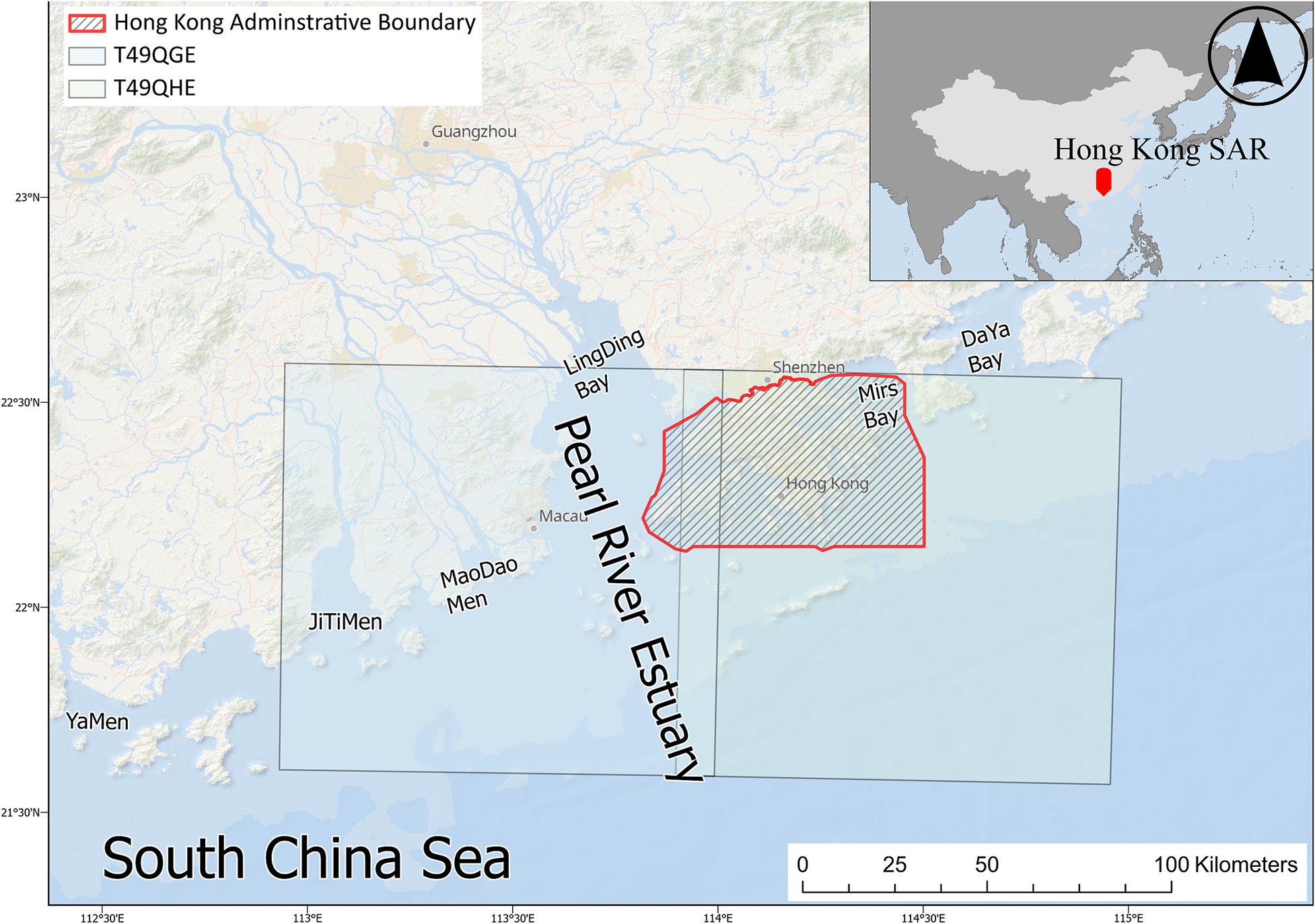
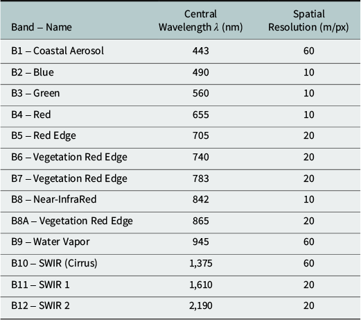
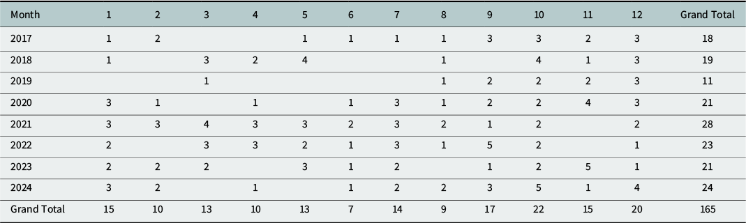
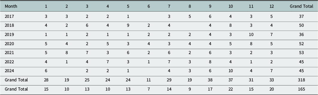
To capture the FMML dynamics in the PRE and HK waters, multispectral imagery from the S2 – MSI was selected as it is a core component of the European Commission’s Copernicus Earth Observation Programme. The multispectral imagery consists of 13 spectral bands (see Table A1 in Appendix A), providing key advantages for coastal and marine applications: a revisiting cycle of around 5 days, swath width up to 200 km and up to 10 m of spatial resolution. S2 emerges as one of the widely discussed and used platforms for satellite-based FMML detecting applications. L1C (Top-Of-Atmosphere, TOA) S2 imagery was acquired via the Copernicus Open Access Hub, in the period from January 2017 to December 2024. To ensure data usability for FMML detection, only products with less than 30% cloud coverage were downloaded. Meanwhile, since HK and the PRE spanned across multiple S2 tiles, the analysis focused on tiles T49QGE and T49QHE (Figure 1). A total of 483 images had been acquired over the study period for temporal spatial analysis, see Appendix B, Tables B1 and B2 for the detailed list of images for each month.
The area of study and the spatial coverage of the two Sentinel-2 tiles of interest.

All downloaded satellite frames underwent the Rayleigh correction function from the SNAP program, developed by the European Space Agency. This is a critical step for maintaining consistency with MARIDA benchmark: the RF classifier was trained on Rayleigh-corrected S2 L1C data (Kikaki et al., Reference Kikaki, Kakogeorgiou, Mikeli, Raitsos and Karantzalos2022) rather than on fully atmospherically corrected products. Different atmospheric corrections would alter the bottom-of-atmosphere (BOA) reflectance, breaking the assumptions of the trained model. Preliminary tests with Sen2Cor corrected L2A products indeed showed noticeably degraded performance. In addition, Hu (Reference Hu2021, Reference Hu2022, Reference Hu2025) showed that standard coastal atmospheric correction generally assumes negligible NIR–SWIR water-leaving reflectance. This is not valid for pixels containing floating material and can introduce substantial artifacts. Next, bands 9 (water vapor) and 10 (Cirrus) were also excluded from the Rayleigh-corrected products, since they contribute little to no values for FMML detection. Furthermore, all other bands are re-sampled to 10 m resolution to align with training data’s quality.
Two types of features were extracted from the Rayleigh-corrected products, as they can enhance the ability to separate FMML from the background waters. In particular, spectral indices (SIs) can help specific spectral contrast between oceanic features and background waters, and are expected to enhance classification performance (Waqas et al., Reference Waqas, Wong, Stocchino, Abbas, Hafeez and Zhu2023). Eight SIs were computed using the definition reported in Appendix A. Moreover, Gray-Level Co-Occurrence Matrix (GLCM) features can help capture the textual patterns, which include six standard features, such as contrast, dissimilarity, homogeneity, energy, correlation, and angular second moment. First, a gray image composite was created with a weighted average method applied to the S2 RGB channels (bands 4, 3, 2) according to Van der Walt et al. (Reference Van der Walt, Schönberger, Nunez-Iglesias, Boulogne, Warner, Yager, Gouillart and Yu2014). A sliding window of 13 × 13 pixels (approximately 130 × 130 m) was created based on each pixel. The gray-level values were then discretized into 16 bin levels for each sliding window, and co-occurrence matrices were calculated at four directions, 0° (east), 45° (northeast), 90° (north), and 135° (northwest). The directional matrices were averaged to achieve rotational-invariant representations, from which six texture features were derived.
MARIDA framework and processing workflow
Once the image datasets have been preprocessed, as described in the previous section, we employed the algorithm described in Kikaki et al. (Reference Kikaki, Kakogeorgiou, Mikeli, Raitsos and Karantzalos2022).
To evaluate the proper algorithm for local FMML detection, two main algorithms, Random Forest (RF) and U-Net, were employed and compared within different datasets. RF is a classic algorithm that includes multiple decision trees for classification, as well as application to regression fitting. RF in this study was performed using 25 features: 11 S2 Spectral Signature (SS) bands, 8 SI, and 6 GLCM features, which provided additional information for each pixel’s properties. The feature collection consisted of a 25-layer description for each pixel. The RF algorithm then classified each pixel into pre-defined categories generated by a combination of decision trees. Within each tree, a random subset of features was used at each node to split data, which can reduce over-fitting and improve generalization. Then, the final label assignment for each pixel was obtained by majority voting across all the decision trees.
A state-of-the-art U-Net model has also been adopted and trained with the MARIDA dataset. The U-Net algorithm has been modified to employ 11-band patches with dimensions of 256 × 256 pixels, and it does not require inputs from SI and GLCM. The architecture was based on an encoder and decoder convolutional neural network, with four convolutional layers. At each of the encoding paths, successive convolutional and pooling layers progressively reduce the size of the input, in this case 11-channel images, while extracting hierarchical feature representations, such as edges, textures, and shapes. The number of feature channels also increased from 16, 32, 64, and 128. The decoder path then upsamples the extracted features back to the original resolution. This process mirrors downsampling and includes four upsampling blocks through a bilinear sampling technique. A final 1 $ \times $
1 convolution layer maps the hidden features onto the output classes to generate a per-pixel segmentation mask (labels).
$ \times $
1 convolution layer maps the hidden features onto the output classes to generate a per-pixel segmentation mask (labels).
In this study, we tested the performance of the different detection algorithm using different datasets. In particular, we analyzed the images provided in the MARIDA dataset (Kikaki et al., Reference Kikaki, Kakogeorgiou, Mikeli, Raitsos and Karantzalos2022). Then we assessed the performance of the algorithm using a plastic mesh target deployed in Lesvos Island (Greece) as in Papageorgiou et al. (Reference Papageorgiou, Topouzelis, Suaria, Aliani and Corradi2022), and, finally, using a test case reported in Cózar et al. (Reference Cózar, Arias, Suaria, Viejo, Aliani, Koutroulis, Delaney, Bonnery, Macías, de Vries, Sumerot, Morales-Caselles, Turiel, González-Fernández and Corradi2024) (Piave River (Italy) outflow scene, October 31, 2018).
After the algorithm validations, all the preprocessed local products were imported into the RF classifier, along with their respective SI and GLCM features. Results from each scene were then stored in both shape file and raster format, annotating each of the predictive classes.
Based on the detected FMML labels at the pixel level, spatial–temporal patterns were quantified across different months and seasons. The study area was divided into $ 1\;{\mathrm{km}}^2 $
grids, and two key metrics were calculated, namely the averaged daily FMML density
$ 1\;{\mathrm{km}}^2 $
grids, and two key metrics were calculated, namely the averaged daily FMML density $ {I}_s $
:
$ {I}_s $
:
 $$ {\overline{I}}_s=\frac{1}{N}\sum \limits_{x,y}I\left(x,y\right) $$
where $ I\left(x,y\right) $
is the FMML count at pixel coordinates
$ I\left(x,y\right) $
is the FMML count at pixel coordinates $ \left(x,y\right) $
,
$ \left(x,y\right) $
, $ N $
is the total number of scenes for the study period. The FMML areal density
$ N $
is the total number of scenes for the study period. The FMML areal density $ {C}_T^D $
is then calculated as:
$ {C}_T^D $
is then calculated as:
 $$ {C}_T^D=\sum \limits_{x,y}^{100}{\overline{I}}_s\times \frac{10^{-6}\;{km}^2}{1\;{m}^2} $$
where $ {\sum}_{x,y}^{100}\;{\overline{I}}_s $
is the total of the average FMML count within the
$ {\sum}_{x,y}^{100}\;{\overline{I}}_s $
is the total of the average FMML count within the $ 1{\mathrm{km}}^2 $
gird, as it encompasses
$ 1{\mathrm{km}}^2 $
gird, as it encompasses $ 100\times 100 $
pixels.
$ 100\times 100 $
pixels. $ {C}_T^D $
is measured in ppm similarly to Cózar et al. (Reference Cózar, Arias, Suaria, Viejo, Aliani, Koutroulis, Delaney, Bonnery, Macías, de Vries, Sumerot, Morales-Caselles, Turiel, González-Fernández and Corradi2024), representing an estimate of the FMML relative density, due to the S2 resolution constraints and probabilistic nature of the classifier.
$ {C}_T^D $
is measured in ppm similarly to Cózar et al. (Reference Cózar, Arias, Suaria, Viejo, Aliani, Koutroulis, Delaney, Bonnery, Macías, de Vries, Sumerot, Morales-Caselles, Turiel, González-Fernández and Corradi2024), representing an estimate of the FMML relative density, due to the S2 resolution constraints and probabilistic nature of the classifier.
Results
Analysis of the field survey data
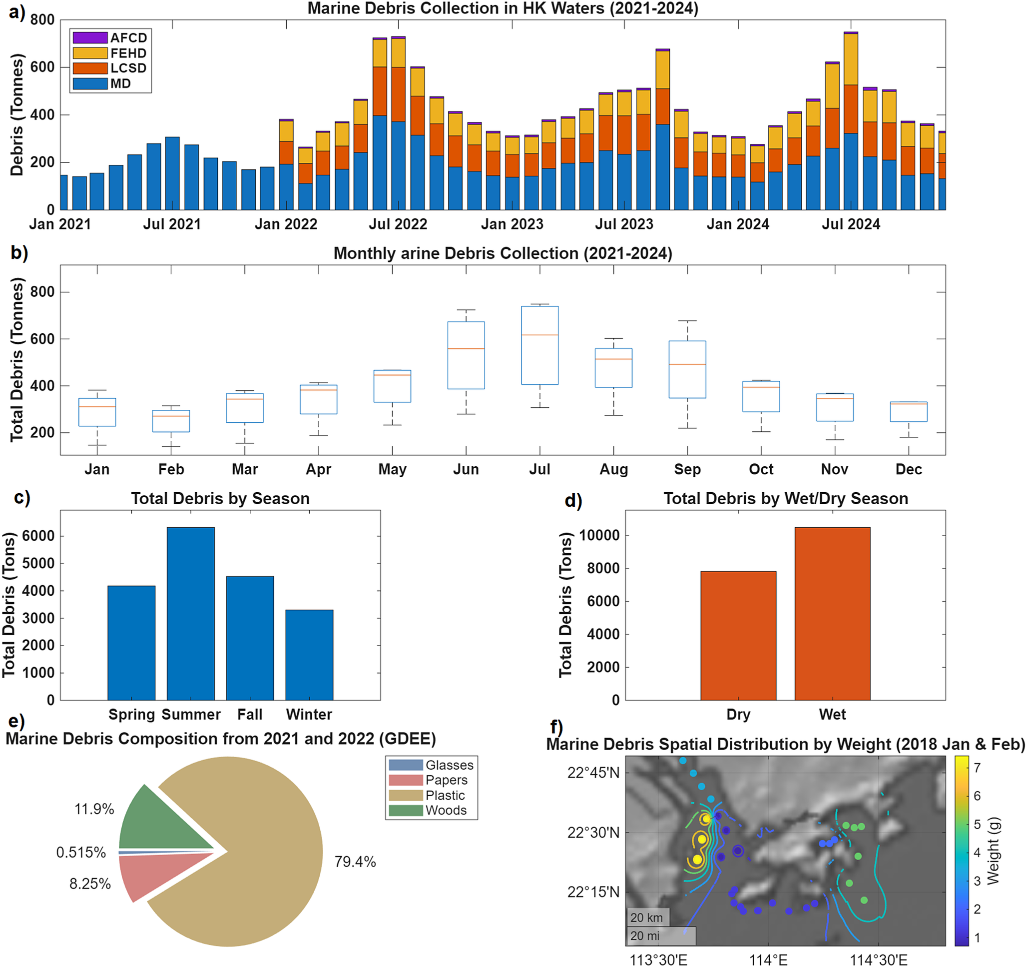
The data collected from land and ocean surveys are shown in Figure 2. The 4-year data from HK EPD have been analyzed with the aim to obtain temporal distribution as shown in panels from (a) to (d). Panel (a) reports the aggregated weight of debris collected (in tons) for MD clean-up campaigns, whereas monthly data have been aggregated and shown as box plots in panel (b) and, finally, seasonal analyses are shown in panels (c) and (d). The data show a strong cyclical temporal variability. The general monthly clean-up quantity ranged from 200 to more than 600 tons monthly, with a noticeable peak during summer periods (July–September). Meanwhile, the wet season (March–August) recorded values up to 10,000 tons of MD, significantly outweighing the amount collected in the dry season. The data from GDEE, shown in panel (e), provide some significant inputs, and their data suggest that the majority of collected FMML is plastic, which aligns with much other local and regional MD-related literature, as well as the global trend (Zhou et al., Reference Zhou, Huang, Fang, Cai, Li, Li and Yu2011; Peng et al., Reference Peng, Dasgupta, Zhong, Du, Xu, Chen, Chen, Ta and Li2019; Zhang et al., Reference Zhang, Wei, Zhang, Zhong, Wang and Jian2022; Liu et al., Reference Liu, Lin, Huang, Yang, Caruso, Baini, Bocconcelli, Rosso and Li2023). As plastic comprises the majority of marine litter, woody debris comes as second, with a composition comes to 11.9% of all debris collected. Papers debris comes as third, with a percentage of 8.25% by count. Glasses count comes as the least, with a percentage of 0.515%.
Post-processed data collected by different sources. (a) and (b) monthly amount of debris collected under the coordination of the Hong Kong Environmental Protection Department between 2021 and 2024. (c) and (d) seasonal cumulative quantities of the same data; (e) classification of the marine litter (source: GDEE); (f) elaboration of the data published by Fok et al. (Reference Fok, Lam, Ng, Li, Yeung and Jia2018) and Lam et al. (Reference Lam, Fok, Lin, Xie, Li, Xu and Yeung2020).

Spatial MD patterns in the PRE were assessed through synthesizing two datasets (Fok et al., Reference Fok, Lam, Ng, Li, Yeung and Jia2018; Lam et al., Reference Lam, Fok, Lin, Xie, Li, Xu and Yeung2020), as the methods employed were directly comparable, and shown in panel (f). The combination of the two datasets reveals a distinct spatial gradient between the eastern and western domains of HK waters, as evidenced by the sampling points collected in January and February 2018. A primary hotspot with MD densities up to $ 7\;\mathrm{g}/{\mathrm{m}}^3 $
can be observed at the western part of the PRE outlet, whereas the upper north of the PRE outlet does not show a high concentration of MD aggregation, with its densities at around
$ 7\;\mathrm{g}/{\mathrm{m}}^3 $
can be observed at the western part of the PRE outlet, whereas the upper north of the PRE outlet does not show a high concentration of MD aggregation, with its densities at around $ 3\;\mathrm{g}/{\mathrm{m}}^3 $
. In the eastern PRE outlet, slight lower MD densities of around
$ 3\;\mathrm{g}/{\mathrm{m}}^3 $
. In the eastern PRE outlet, slight lower MD densities of around $ 1\;\mathrm{g}/{\mathrm{m}}^3 $
can be observed. This relatively low density is consistent across the sampling points in the southern HK waters, where the MD densities are typically around
$ 1\;\mathrm{g}/{\mathrm{m}}^3 $
can be observed. This relatively low density is consistent across the sampling points in the southern HK waters, where the MD densities are typically around $ 2\;\mathrm{g}/{\mathrm{m}}^3 $
. On the other hand, the eastern HK waters exhibit different patterns characterized by moderately high density, with concentrations reaching up to
$ 2\;\mathrm{g}/{\mathrm{m}}^3 $
. On the other hand, the eastern HK waters exhibit different patterns characterized by moderately high density, with concentrations reaching up to $ 5\;\mathrm{g}/{\mathrm{m}}^3 $
.
$ 5\;\mathrm{g}/{\mathrm{m}}^3 $
.
Detection algorithm validation and performance assessment
We started the performance assessment of the RF and U-Net algorithm using the dataset provided in the MARIDA repository (Kikaki et al., Reference Kikaki, Kakogeorgiou, Mikeli, Raitsos and Karantzalos2022) and comparing the statistical metrics defined in Appendix C.
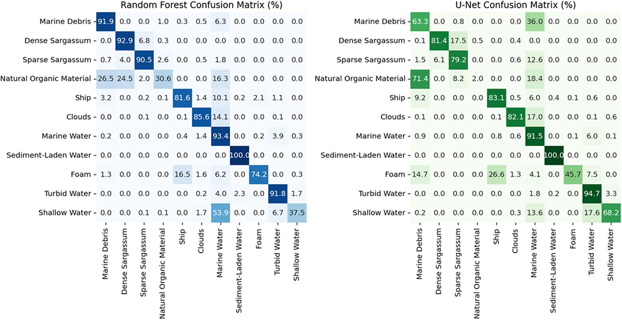
RF achieved a pixel accuracy (PA) of 0.94 and a macro-F1 score of 0.79, outperforming the U-Net model (PA: 0.92, a macro-F1: 0.70). The RF model demonstrated a balanced performance precision (0.69) and recall (0.92), identifying most MD while minimizing false positives. In contrast, the U-Net had a lower precision of 0.32, but a higher recall rate, showing it experiences difficulty in differentiating MD from other classes but yet notice false positives. Figure 3 shows the confusion matrix for the RF classifier and the U-Net model, where the vertical axis is the true labels and the horizontal axis corresponds to the predicted labels. The confusion matrix has been computed for several features other than the MD, which is the main focus in the present study. By inspecting the matrices, the results suggest that RF algorithm produced a much higher percentage of success in terms of number of pixels correctly classified over the total number of pixels for each class. Just focusing on MD, RF reached 91.9% of success compared to 63.3% obtained with U-Net. Most of the misclassified pixels of MD were attributed to Marine Water by both the algorithm, although with very different percentages (RF = 6.3%; U-Net = 36%).
Confusion matrix for the RF classifier and the U-Net model. Numerical values have been converted from pixel counts to percentages. The vertical axis is the true labels, whereas the horizontal axis is the predicted labels.

Based on these tests, we selected the RF algorithm for FMML monitoring due to its better performance.
We then tested the RF classifier on other scenes already analyzed in previous studies (Papageorgiou et al., Reference Papageorgiou, Topouzelis, Suaria, Aliani and Corradi2022; Cózar et al., Reference Cózar, Arias, Suaria, Viejo, Aliani, Koutroulis, Delaney, Bonnery, Macías, de Vries, Sumerot, Morales-Caselles, Turiel, González-Fernández and Corradi2024).
For the first test, we used the real-world scale tests conducted in 2021 nearby the Lesvos Island (Greece) coastline where two artificial targets (a blue High-Density Polyethylene mesh, representing FMML, and an orange wooden target representing Natural Organic Matter) were deployed in summer and in autumn. A scene from June 21, 2021, was selected as the plastic target remained unsubmerged and free from biofouling under calm sea state conditions (<3 m/s wind speed). These conditions provided a more ideal scenario and isolated external environmental noise while testing the RF classifier’s core detection capability. The RF’s performance on this scene remains to be limited. For the nine-pixel plastic target cluster, only one pixel was correctly classified as MD, resulting in a recall of 11.1%. The remaining eight pixels were misclassified, predominantly as cloud and sediment-laden water. In contrast, the RF classifier performs more proficiently on the organic wooden target, with most pixels comprising the wooden target being correctly identified as natural organic material, with some peripheral misclassification into cloud and dense Sargassum. Outside the designated targets, the classifier generated isolated false positives for MD and cloud in adjacent open waters. Visual inspection of high-resolution RGB channels confirmed no actual floating objects at these locations. These false positives arose due to spectral noise or ambiguous water surface features, a common challenge in automated detection. Critically, this finding highlights the need for caution when applying the RF classifier to complex coastal environments.
The second test was performed using a scene from the North Adriatic Sea (Italy) at the Piave River outflow, captured on October 31, 2018 (Cózar et al., Reference Cózar, Arias, Suaria, Viejo, Aliani, Koutroulis, Delaney, Bonnery, Macías, de Vries, Sumerot, Morales-Caselles, Turiel, González-Fernández and Corradi2024). The RF classifier successfully detected the FMML strip, identifying its central core of accumulation and correctly classified most of the pixels as MD. This confirms the RF’s ability to detect large aggregations of FMML in a complex, dynamic coastal environment, even with sun glint. The classification also revealed the heterogeneous composition of the FMML, as some pixels were labeled as dense Sargassum and natural organic material, a mixture of anthropogenic debris and natural matter. The classifier also accurately labeled the sediment plume and clouds.
Together with the Lesvos island test scene, these results highlight the RF’s capabilities and limitations: strong performance in detecting large FMML accumulations (e.g., river outflows) but challenges with small, isolated targets. False positives in both cases underscore the need for cautious interpretation in complex conditions.
FMML detection in Hong Kong and PRE waters (2017–2024)
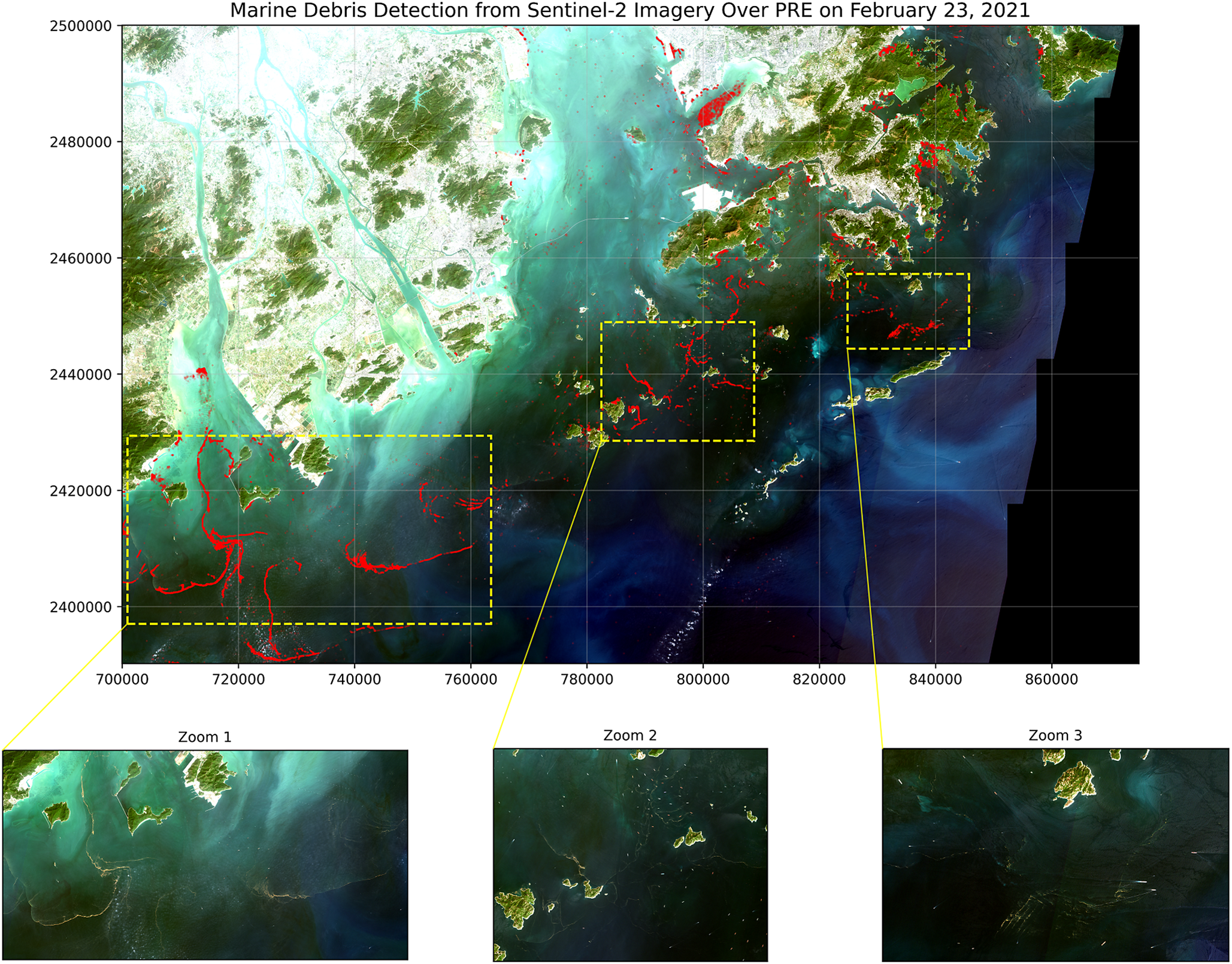
The trained RF classifier was deployed on 2017–2024 S2 imagery, focusing on tiles T49QGE and T49QHE. An example of the results of the classification based on the RF algorithm on February 23, 2021, is shown in Figure 4. The pixel classified as FMML is reported in red over the satellite tiles mosaiced. The example shows a case with relatively high content of FMML concentrated in well-organized patches and filaments. We will discuss later on a possible physical explanation of the debris distribution.
An example of the FMML detection over tile T49QGE and T49QHE, utilizing the MARIDA-trained RF classifier on February 23, 2021.

Adopting density calculation methods from Cózar et al. (Reference Cózar, Arias, Suaria, Viejo, Aliani, Koutroulis, Delaney, Bonnery, Macías, de Vries, Sumerot, Morales-Caselles, Turiel, González-Fernández and Corradi2024), the FMML accumulation plot and spatial–temporal density maps will be expressed in part per million (ppm) using equation 2. We aggregated the results in terms of monthly averages and seasonal averages.
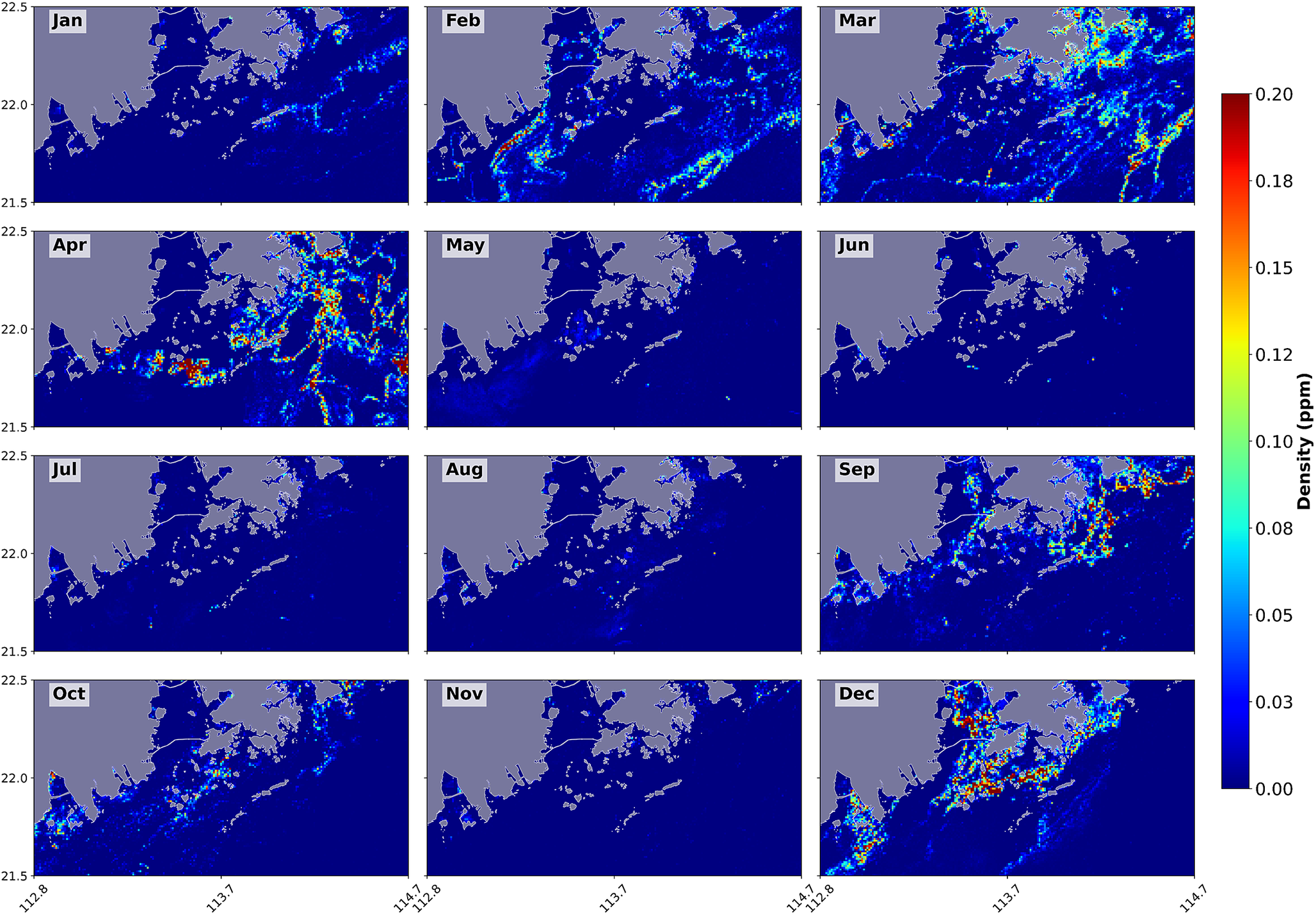
Regarding the monthly averaged distribution, Figure 5 shows the results of the computed FMML concentrations.
Monthly maps of FMML mean concentration of the period under investigation.

The monthly distribution of PRE FMML and adjacent waters exhibits significant spatial–temporal variability. In January, minimal FMML presence is observed, showing only a few isolated detections (0.1 ppm) in the eastern HK open waters. A distinct transport pathway emerges in February, forming a transect at around 0.4 ppm at the southern PRE outlet, and extends southeastward, passing MaoDaoMen and JiTiMen before spreading offshore. In March, this continuous FMML front dissipates, giving way to higher concentrations in the northeastern estuarine outlet and eastern open water. Additionally, a slight FMML travel pattern is noted near the western YaMen outlet. In April, the accumulation of FMML is noticeable around the latitude of 22.0°N in the western part of the study area, particularly south of the estuarine outlying islands, with densities up to 0.8 ppm, and minimal FMML at the estuarine outlet. However, a higher density of FMML can be observed across the entire eastern domain, with three filament-like structures. From May to August, the abundance of FMML is typically low, with only sporadic occurrences noted across the region. In May, a faint and low-density debris filament shows a southwestward path originating from the estuary. Throughout mid-summer, only occasional accumulations are recorded near JiTiMen and YaMen. In September, a reappearing debris filament front from the northeastern estuary shows a lower concentration of 0.07 ppm compared to February, with this structure gradually shifting southwest toward the outlying islands. An additional FMML front has formed between 22.0°N and 22.5°N in the western region, marked by higher-density hotspots near the shoreline. In the eastern area, FMML accumulations extend from DaYa Bay to Mirs Bay and continue south along the HK coast. Notably, high FMML density is found at the outer edges of the transect belts rather than closer to shore. In October, a light FMML belt forms around 21.8–22.0°N near the southern estuarine outlying islands, with further concentrations along the coastline. A lower-density FMML belt extends south from Mirs Bay into the eastern waters. Compared to September, both the amount and intensity of FMML have decreased. By November, the FMML had diminished significantly, although a small amount could still be found in the DaYa Bay. In December, FMML becomes widely distributed across the domain, particularly in the eastern estuary. High concentration can be observed near 21.8°N and 113.5°E, reaching levels up to 0.5 ppm. In contrast, the eastern domain exhibits only minor high FMML concentrations, although a slight accumulation strip is noted as it moved from the eastern HK waters along the southern coast, accumulating again around the outlying islands at 21.8–22.0°N, where densities reach around 0.4 ppm. This front eventually merges with the one coming from the estuarine outlet. On average, the eastern waters is observed to deviate from the western waters. In the eastern region, the FMML is generally found closer to the shore, with scattered patches also present in open water.
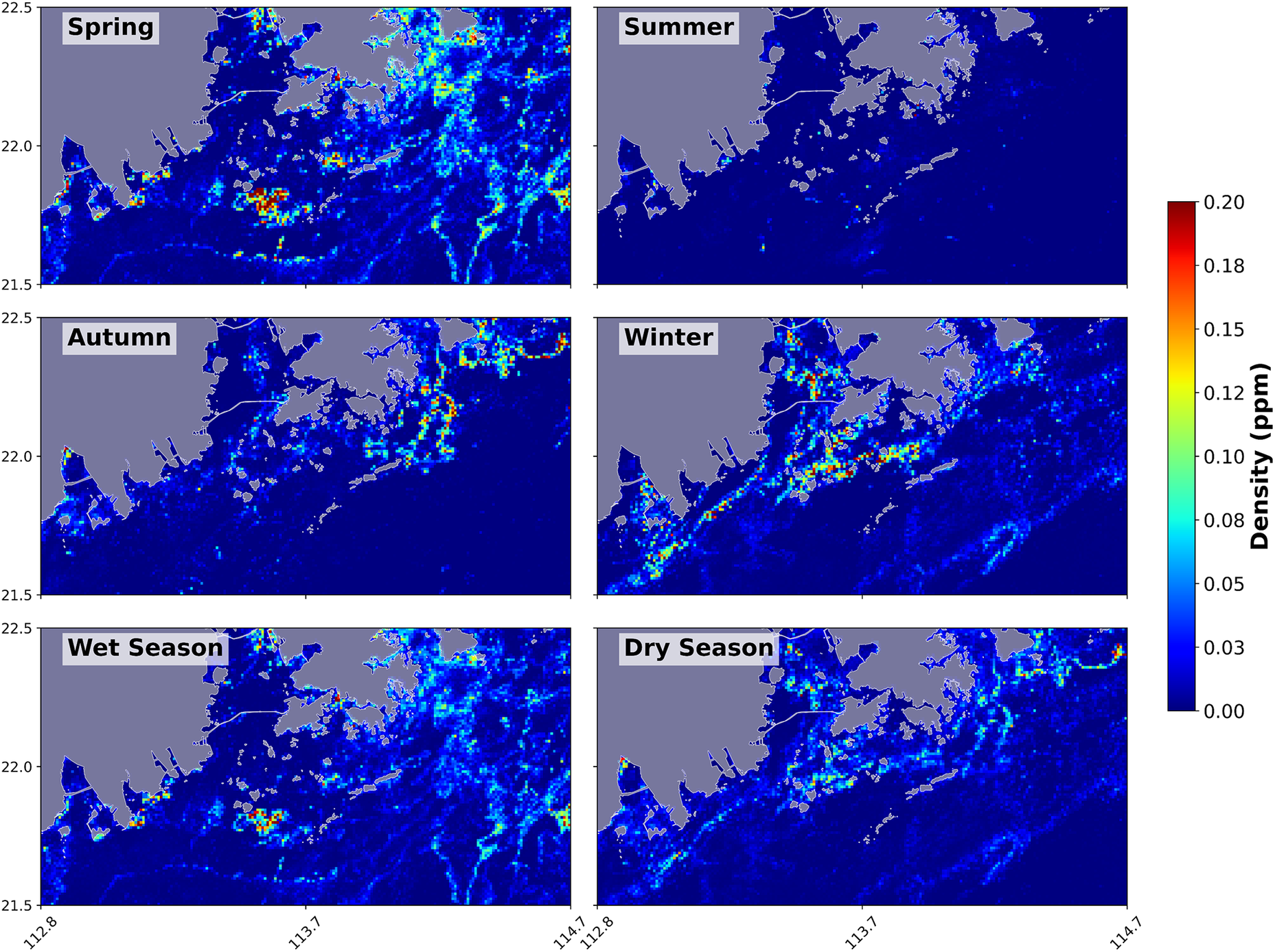
To further understand the seasonal dynamics of FMML accumulation, results were aggregated into climatological and monsoon seasons (dry and wet seasons), see Figure 6. In springtime, FMML is distributed across the entire study area. However, the eastern domain exhibits even dispersion (at around 0.2 ppm), with a higher density (0.4 ppm) at the estuarine outlying islands. The highest concentrations of FMML are predominantly found along the latitudinal transect of 21.8°N–22.0°N, while the estuary and HK inner harbor lack distinct patterns. During summer, only isolated high-density patches exist, with no widespread patterns being observed. In autumn, a prominent FMML belt (at around 0.1 ppm) forms northeast of the estuary, extending southeast through western open water and outlying islands before scattering westward. Minor accumulations also appear along the coastline between 113.2°E and 113.5°E. The eastern domain features a nearshore FMML belt, resembling the September pattern. This belt stretches from DaYa Bay to Mirs Bay, and south along HK’s shoreline with relatively uniform density. In winter, patterns similar to December reappear, with an FMML belt crossing the estuarine outlet and connecting with another belt from the eastern domain, which migrates southwest along the coast. For the wet season, FMML is widespread across the eastern domain but generally diffuse, with occasional high spots of around 0.2 ppm. Interestingly, the PRE river outlet remains relatively clean. Yet the surrounding islands in the PRE outlet, the northeastern corner of the river outlet, particularly inlets of Hong Kong Harbor, and the JiTiMen outlets show high accumulation during wet months.
Seasonal maps of FMML mean concentration of the period under investigation.

In the dry season, an FMML belt originating from the center of the PRE outlet travels southward, migrating southwest along the western HK coastline and continuing through the outlying islands into open water. In the eastern domain, another FMML belt, parallel to the coastline, can be observed, similar to autumn pattern. Interestingly, although there is not much high density of FMML points in the dry season, a clear potential transport pathway is evident.
Discussion
Seasonal and monthly distribution: Difference between remote sensing observations and field sampling
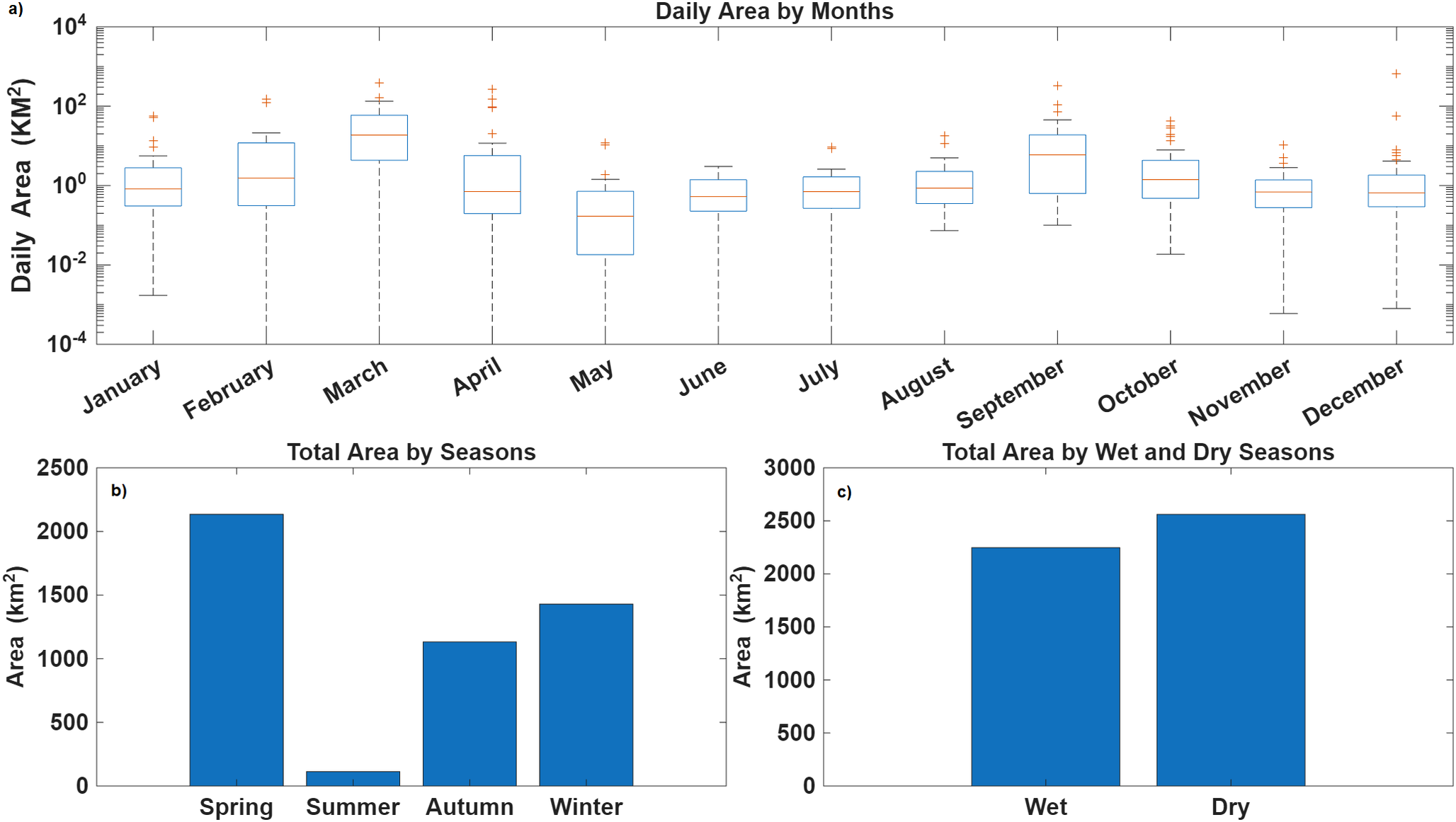
We now compare the results obtained by the multi-year remote sensing analysis and the field observation presented in the previous section. To this end, we aggregated the data producing box plots for each month using the daily FMML abundance observed, see Figure 7, panel (a), and the corresponding seasonal distribution, Figure 7, panels (b) and (c). Examining the monthly FMML distributions, satellite-derived abundance clearly indicates higher values in March and September, panel (a). In March, the onset of the wet season after several dry winter months is likely to have produced a first-flush effect, whereby intense rainfall mobilized accumulated debris from land areas and riverbanks into the estuary, a mechanism analogous to suspended sediment and nutrient fluxes in the PRE (Ma et al., Reference Ma, Wang, Chen and Zhang2025). Meanwhile, September peaks seem to be driven by the transitional circulation patterns, including the interaction of easterly winds, tidal currents, as well as relatively high rainfall. These forces result in a seaward migration of debris or its recirculation offshore, exhibiting behaviors that are similar to river plume transport (Ma et al., Reference Ma, Wang, Chen and Zhang2025). This may explain its southeast trajectory in the PRE outlet, as well as the unique angular shape in the eastern domain along the coastline. Conversely, FMML levels exhibited a decline during the summer months, from April to August. In the seasonal distributions, panels (b) and (c), there is a net predominance of Spring and wet season over the other period of the year. This phenomenon may be indicative of a seasonal shift in the pathways of FMML. Strong southwestern winds, elevated wave energy, and typhoon activity are believed to drive debris ashore, thereby increasing beach accumulation rather than the presence of floating debris. Reports from the HK EPD confirm this argument, documenting peak beach clean-up volumes during the summer months, see Figure 2, panels (a) and (b). These findings align with recognized hydrodynamic patterns and support previous research that identified accumulation hotspots in HK’s eastern waters (EPD, 2025; Lam et al., Reference Lam, Fok, Lin, Xie, Li, Xu and Yeung2020). Meanwhile, the decoupling between satellite-detected FMML peaks (March, September) and beach clean-up peaks (summer) underscores a fundamental challenge in satellite-based debris monitoring: sensors only detect the surface debris that surpasses pixel-scale thresholds at the time of overpass, while ground surveys account for both stranded and submerged debris over extended periods. Therefore, the mismatch arises from differences in sampling methods and temporal coverage as much as from classifier limitations.
(a) Box plots of the daily data detected for each month; (b) and (c) seasonal averages.

Regarding the spatial distribution, we might attempt a comparison between the present results and the ones described in Fok et al. (Reference Fok, Lam, Ng, Li, Yeung and Jia2018) and Lam et al. (Reference Lam, Fok, Lin, Xie, Li, Xu and Yeung2020) and shown in Figure 2, panel (f). The highest concentration reported is on the west bank of the PRE, where our results show a very low content of FMML. The apparent discrepancy could be related to the target plastic debris collected during the field surveys. Indeed, the collected debris had a size impossible to be detected from remote sensing, even at relatively high concentration.
Marine debris distribution and its link to Lagrangian circulation patterns
The spatial discrepancy observed in the FMML concentration further demonstrates the need to investigate the role of hydrodynamic processes in governing the transport and accumulation of MD within the estuary. To this end, we attempted to link the observed superficial distributions using a Lagrangian description of the local circulation in terms of the so-called LCSs. LCSs may play a dominant role in controlling the accumulation and spreading of marine pollutants (Olascoaga and Haller, Reference Olascoaga and Haller2012; Peng et al., Reference Peng, Xu, Shao, Weng, Niu, Li, Zhang, Li, Zhong and Yang2024). Two major classes of LCSs are known to shape the spatial distribution of the pollutant, namely the attracting structures, which tend to aggregate the mass along them, and the repelling structures that conversely tend to spread the mass away. The dynamical interplay between these two opposite Lagrangian flow behaviors often explains the observed pollutant large-scale patterns.
The spatiotemporal analysis indicates that FMML does not disperse evenly but accumulates in recurrent ocean sub-domains that are likely shaped by monthly/seasonal hydrodynamic processes. In the western region, offshore transport emerges during late winter and autumn. In contrast, the eastern region shows stronger and more persistent nearshore accumulations, especially in winter. Specifically, the spatial patterns suggest that MD originates from the central and western parts of the estuary and then disperses in a southwestern direction across the study area. The local circulation is dominated by wind and tidal forcing, multi-island bathymetry – especially at the exit of the PRE in the HK waters – monsoon-driven stratification, and persistent freshwater inputs from the PRE, generating significant seasonal variations in both vertical mixing and sub-10 km energy transfers (De Leo and Stocchino, Reference De Leo and Stocchino2022, Reference De Leo and Stocchino2023; He et al., Reference He, Yin, Stocchino, Wai and Li2022, Reference He, Yin, Stocchino and Wai2023). Moving closer to the nearshore area of the PRE and HK waters, energetic submesoscale currents, influenced by astronomical tides and seasonal monsoons, interact with the bathymetry generating eddies and anisotropic elongated fronts and filaments with potential impact on the local water quality (De Leo et al., Reference De Leo, Tambroni and Stocchino2022; He et al., Reference He, Yin, Stocchino, Wai and Li2022, Reference He, Yin, Stocchino and Wai2023). This extremely active hydrodynamics may generate persistent Lagrangian patterns and, in particular, intense LCSs. LCS in the PRE has been recently investigated showing both repelling and attracting structures along the longitudinal direction of the estuary (Wei et al., Reference Wei, Zhan, Cai, Zhan and Ni2018). The existence of LCSs in the PRE has been recently investigated showing the appearance of both repelling and attracting LCS along the longitudinal direction of the estuary (Wei et al., Reference Wei, Zhan, Cai, Zhan and Ni2018). To verify the possible effect of LCSs on the floating litter distribution as shown in Figures 5 and 6, we computed the Finite Time Lyapunov Exponent ( $ FTLE $
) fields following the methodology used by De Leo et al. (Reference De Leo, Enrile and Stocchino2022) for computing repelling and attracting LCS starting from the high-resolution hydrodynamic simulations used in previous studies (about 200 m) (He et al., Reference He, Yin, Stocchino, Wai and Li2022, Reference He, Yin, Stocchino and Wai2023). LCSs have been computed with 30 m resolution that is close to the satellite image resolution, leading to an accurate identification of the main Lagrangian structures. From this point of view, both observation and Lagrangian analysis can be helpful in explaining the overall patterns and pathways of FMML, leaving unanswered smaller-scale processes such as fragmentation, which would require a much higher resolution.
$ FTLE $
) fields following the methodology used by De Leo et al. (Reference De Leo, Enrile and Stocchino2022) for computing repelling and attracting LCS starting from the high-resolution hydrodynamic simulations used in previous studies (about 200 m) (He et al., Reference He, Yin, Stocchino, Wai and Li2022, Reference He, Yin, Stocchino and Wai2023). LCSs have been computed with 30 m resolution that is close to the satellite image resolution, leading to an accurate identification of the main Lagrangian structures. From this point of view, both observation and Lagrangian analysis can be helpful in explaining the overall patterns and pathways of FMML, leaving unanswered smaller-scale processes such as fragmentation, which would require a much higher resolution.
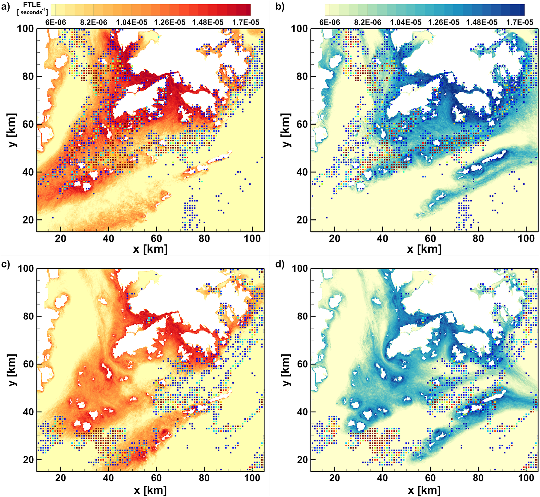
Two examples of superposition of the computed attracting and repelling $ FTLE $
fields with the detected FMML distribution are shown in Figure 8 for December 2017 (panels (a) and (b)), and April 2017 (panels (c) and (d)). The results suggest that the FMML distribution nicely aligns with the strong signal of FTLE marking the presence of attracting LCS, especially in December, panel (a). It is also interesting to note how the high FMML concentration observed in the south waters remains always surrounded by attracting and repelling LCS, possibly leading to a longer persistence in those water sub-basins. It is also interesting to note how the west side of the PRE remains relatively clean (low to zero FMML concentration) where LCS are detected with the exception of the centerline of the estuary, in accordance with Wei et al., Reference Wei, Zhan, Cai, Zhan and Ni2018. The present prediction is in line with previous Lagrangian analysis where the trajectories of floating drifters have been reported (Gu et al., Reference Gu, Zhang, Tuo, Hu, Chen and Hu2024, Reference Gu, Zhang, Sui and Chen2025).
$ FTLE $
fields with the detected FMML distribution are shown in Figure 8 for December 2017 (panels (a) and (b)), and April 2017 (panels (c) and (d)). The results suggest that the FMML distribution nicely aligns with the strong signal of FTLE marking the presence of attracting LCS, especially in December, panel (a). It is also interesting to note how the high FMML concentration observed in the south waters remains always surrounded by attracting and repelling LCS, possibly leading to a longer persistence in those water sub-basins. It is also interesting to note how the west side of the PRE remains relatively clean (low to zero FMML concentration) where LCS are detected with the exception of the centerline of the estuary, in accordance with Wei et al., Reference Wei, Zhan, Cai, Zhan and Ni2018. The present prediction is in line with previous Lagrangian analysis where the trajectories of floating drifters have been reported (Gu et al., Reference Gu, Zhang, Tuo, Hu, Chen and Hu2024, Reference Gu, Zhang, Sui and Chen2025).
Monthly average FTLE fields together with the corresponding FMML distribution. (a) attracting $ FTLE $
fields computed in December 2017; (b) repelling
$ FTLE $
fields computed in December 2017; (b) repelling $ FTLE $
fields computed in December 2017; (c) attracting
$ FTLE $
fields computed in December 2017; (c) attracting $ FTLE $
fields computed in April 2017; (d) repelling
$ FTLE $
fields computed in April 2017; (d) repelling $ FTLE $
fields computed in April 2017.
$ FTLE $
fields computed in April 2017.

Challenges in model generalization and transfer learning
The MARIDA-trained RF classifier outperformed the U-Net model in operational FMML monitoring, with performance metrics that reflect its greater reliability for complex coastal environments like the present study area. This superior performance stems from the RF’s ensemble learning structure and its integration of physics-based features: SIs (e.g., FDI, for plastic-specific detection; NDVI, for excluding vegetation) and GLCM textural features (e.g., contrast, homogeneity) that encode in situ scientific knowledge of FMML’s optical properties. These features enhance discriminative power for complex oceanic scenes and offer high interpretability. In contrast, the U-Net relies solely on raw S2 bands, learning linear correlations from training data that may fail to generalize to new environments, where optical and hydrodynamic conditions differ drastically. Despite its strengths, the RF’s generalization capability remains limited, as evidenced by two key external validation cases. In the test scene provided in Papageorgiou et al. (Reference Papageorgiou, Topouzelis, Suaria, Aliani and Corradi2022), the RF showed weak recall for small plastic targets (11.1% recall). Conversely, in the Italy Piave River test, the model successfully detected a large FMML transect. This dual performance highlights the RF strength in identifying large-scale FMML aggregations but weakness in detecting small, isolated debris.
A key challenge is pixel purity, as a Sentinel-2 pixel labeled as FMML rarely consists entirely of litter. Instead, it typically includes a small, variable amount of debris mixed with water, foam, and other substances. In such mixed pixels, the plastic signal is spectrally diluted, reducing separability from background water and making the classifier particularly prone to false negatives when aggregations are small or sparse. A similar mechanism has been reported for artificial targets (Papageorgiou et al., Reference Papageorgiou, Topouzelis, Suaria, Aliani and Corradi2022) and in theoretical analyses of sub-pixel detection limits (Hu, Reference Hu2021). The trained RF model is therefore more sensitive to large, coherent aggregations (e.g., the Piave plume) than to small targets such as the PLP-2021 mesh, and this directly affects how the ppm metric should be interpreted. Consequently, the ppm values reported here are “relative” surface FMML abundance rather than absolute concentrations, particularly when sub-pixel coverage dominates.
The extension of the trained RF algorithm demonstrated potential difficulties which can be summarized as follows. First, atmospheric variability between the training dataset and the actual application may disrupt spectral consistency. MARIDA data have been collected under calm sea states and clear atmosphere, while on the contrary, the PRE experiences highly variable aerosol loads from industrial, urban, and biomass burning sources (Jin et al., Reference Jin, Ma, Huang, Huang, Gong, Liu, Wang, Fan and Li2023; Liu et al., Reference Liu, Li, Lin, Guo, Yuan, Yang and Zhai2024), and water vapor. Even after the Rayleigh correction, residual atmospheric effects can distort SSs and generate false positives. At the same time, comprehensive coastal atmospheric correction (e.g., NIR–SWIR-based water-leaving retrievals) is not a suitable solution: Hu (Reference Hu2021, Reference Hu2022, Reference Hu2025) showed that such schemes often over-correct pixels containing floating material because they assume negligible NIR water-leaving reflectance. In this case, using Rayleigh-corrected reflectance and analyzing relative differences between target pixels and nearby water can be more appropriate than potentially overestimated BOA reflectance.
Second, dynamic debris characteristics alter SSs not captured by MARIDA. FMML’s spectral profile is not static, as plastic types, weathering, submersion level, pixel coverage, and biofouling modify S2 reflectance (Min et al., Reference Min, Cuiffi and Mathers2020; Belone et al., Reference Belone, Kokko and Sarlin2022; Papageorgiou et al., Reference Papageorgiou, Topouzelis, Suaria, Aliani and Corradi2022). MARIDA’s plastic targets exhibit distinct peaks in Band 8 and 8A. Moreover, Napper and Thompson (Reference Napper and Thompson2020) noted that China’s polymer inputs and local weathering processes could create SSs that differ from those in global datasets like MARIDA and lead the RF to misclassify plastics. Third, the PRE’s water dynamics could create a background different from MARIDA’s training data. The PRE’s dynamics in aquatic environments (Niu et al., Reference Niu, Cai, Jia, Luo, Tao, Dong and Yang2021; Ma et al., Reference Ma, Wang, Chen and Zhang2025) drive high turbidity and sediment mixing, which disrupts the FMML SS and makes it less obvious for RF to distinguish. Meanwhile, the RF has also become overtrained to MARIDA’s Rayleigh-corrected reflectance, only recognizing FMML signatures with the specific atmospheric state of training images. When RF is exposed to the PRE’s different atmospheric conditions, this overspecialization might further degrade performance.
Conclusion and future directions
This study highlights both the significant potential and the limitations of using the trained RF classifier for monitoring FMML in the environmentally complex PRE. The RF models prove to be a robust tool for large-scale detection, effectively identifying major spatial–temporal patterns that correspond with known hydrodynamic drivers. However, there is a discrepancy between the FMML peaks derived from satellite data and the summer maxima found in ground-collected data. This difference may indicate a dynamic that the RF classifier cannot detect, leading to an underestimation of true abundance during times of high hydrodynamic energy. This underestimation can occur due to rapid debris dispersion, submergence, or beach stranding (Vorsatz et al., Reference Vorsatz, So, Cheung, Not and Cannicci2025). The main issue identified is that the model has limited generalization capabilities when encountering the unique atmospheric and water conditions of the PRE. Challenges such as aerosol interference, turbid waters, and the presence of region-specific debris signatures can result in false positives and compromise the accuracy of detection. Therefore, although the tuned RF classifier offers a promising solution, its practical application needs to extend beyond a straightforward transfer-learning approach. Moreover, the spatial distribution detected using the satellite images is well described by the FTLE fields computed starting from the local circulation.
Based on the present findings, future research and algorithm development, including machine learning models, should focus on three main goals: enhancing model robustness to atmospheric variability, considering the dynamic nature of MD, and integrating hydrodynamic conditions. For example, it would be necessary to address atmospheric conditions by revising MARIDA data inputs. Since MARIDA excludes S2 Bands 9 and 10, critical for accurate atmospheric characterization, future datasets and models could incorporate these bands to better measure aerosol conditions. Alternatively, develop models using TOA radiance, as atmospheric correction itself can introduce errors. This approach may resolve aerosol-related challenges without relying on in situ efforts. Second possible line of research could be exploring hybrid modeling approaches by integrating remote sensing detection with external environmental data. Following the framework outlined by Cózar et al. (Reference Cózar, Arias, Suaria, Viejo, Aliani, Koutroulis, Delaney, Bonnery, Macías, de Vries, Sumerot, Morales-Caselles, Turiel, González-Fernández and Corradi2024), combining S2 with wind, current and their Lagrangian properties, and physical data as additional input with spectral SI could substantially improve classifier performance. Third, enhancing FMML detection via information integration such as coupling physical tracking with hydrodynamic simulations to predict FMML pathways.
Open peer review
To view the open peer review materials for this article, please visit http://doi.org/10.1017/plc.2026.10049.
Data availability statement
Replication data and code will be made available on request.
Author contribution
Conceptualization: F.L.; A.S.; Data curation: F.L., A.D.L.; Data visualization: F.L., A.D.L.; Methodology: F.L., A.S., M.S.W.; Writing original draft: F.L. All authors approved the final submitted draft.
Financial support
This research was supported by grants from the Research Grants Council of HK (project IDs 15216422, AoE/P-601/23-N). M.S. Wong thanks the support from the General Research Fund (Grant No. 15603923 and 15609421), and the Collaborative Research Fund (Grant No. C5062-21GF) and Young Collaborative Research Fund (Grant No. C6003-22Y) from the Research Grants Council, Hong Kong, China. He also acknowledged the funding support (Grant No. N-ZH8S, BBG2, and 1-CDL5) from the Otto Poon Research Institute for Climate-Resilient Infrastructure, Research Institute for Sustainable Urban Development, Research Institute of Land and Space, The Hong Kong Polytechnic University, Kowloon, Hong Kong, China.
Competing interests
The authors declare no competing interests.
Appendix A: Spectral bands and indices
The spectral indices employed in the preprocessing of the satellite images are defined as follows:
 $$ {\displaystyle \begin{array}{l}\mathrm{Normalized}\ \mathrm{Different}\ \mathrm{Vegetation}\ \mathrm{Index}: NDVI\hskip0.3em =\hskip0.3em \frac{B8-B4}{B8+B4}\end{array}} $$
 $$ {\displaystyle \begin{array}{l}\mathrm{Floating}\ \mathrm{Algae}\ \mathrm{Index}:\hskip1em FAI=B8-B4-\left(B11-B4\right)\times \frac{\lambda_8-{\lambda}_4}{\lambda_{11}-{\lambda}_4}\end{array}} $$
 $$ {\displaystyle \begin{array}{l}\mathrm{Floating}\ \mathrm{Debris}\ \mathrm{Index}: FDI\hskip0.3em =\hskip0.3em B8-B6+\left(B11-B6\right)\\ {}\times \frac{\lambda_8-{\lambda}_6}{\lambda_{11}-{\lambda}_6}\times 10\end{array}} $$
 $$ {\displaystyle \begin{array}{l}\mathrm{Shadow}\ \mathrm{Index}:\hskip.2em ShI=1-\sqrt{\left(B2\times B3\times B4\right)}\end{array}} $$
 $$ {\displaystyle \begin{array}{l}\mathrm{Normalized}\ \mathrm{Difference}\ \mathrm{Wetness}\ \mathrm{Index}\hskip1em NDWI=\frac{B3-B8}{B3+B8}\end{array}} $$
 $$ {\displaystyle \begin{array}{l}\mathrm{Normalized}\;\mathrm{Red}\;\mathrm{Difference}\ \mathrm{Index}\hskip2em NRD=\frac{B8-B5}{B8+B5}\end{array}} $$
 $$ {\displaystyle \begin{array}{l}\mathrm{Normalized}\ \mathrm{Difference}\ \mathrm{Moisture}\ \mathrm{Index}\hskip2em NDMI\hskip1em =\frac{B8-B11}{B8+B11}\end{array}} $$
 $$ {\displaystyle \begin{array}{l}\mathrm{Bare}\ \mathrm{Soil}\ \mathrm{Index}\hskip2em BSI=\frac{\left(B4+B11\right)-\left(B8+B2\right)}{\left(B4+B11\right)+\left(B8+B2\right)}\end{array}} $$
Spectral bands and technical specifications of Sentinel-2 MSI. Bands 9 and 10 are excluded from FMML detection, while all other bands are retained for feature extraction

Appendix B: Details on Sentinel-2 images downloaded
Number of cloud-free ( $ \le $
30%) Sentinel-2 images for T49QGE
$ \le $
30%) Sentinel-2 images for T49QGE

Number of cloud-free ( $ \le $
30%) Sentinel-2 images for T49QHE
$ \le $
30%) Sentinel-2 images for T49QHE

Appendix C: Statistical metrics
-
• Intersection-over-Union ( $ IoU $
):
$ IoU $
):

 $$ IoU= TP/\left( TP+ FP+ FN\right), $$
where $ TP $
is the number of true positives,
$ TP $
is the number of true positives, $ FP $
the number of false positives, and
$ FP $
the number of false positives, and $ FN $
the number of false negatives.
$ FN $
the number of false negatives.
-
• Precision (
$ P $
):

 $$ P= TP\left( TP+ FP\right) $$
-
• Recall (
$ R $
):

 $$ R= TP\left( TP+ FN\right) $$
-
• The
$ {F}_1 $
score is defined as the harmonic mean between the precision
$ P $
and the recall
$ R $
. -
• Pixel Accuracy (PA) is the ratio of the correctly predicted pixels to the total number of pixels.


 Open access
Comments
Dear Editor,
first of all, I apologize for the delay in the submission of this invited paper.
we are submitting the manuscript entitled “Beyond the pixel: multi-year tracking of Floating Marine Litter from satellite images” where we report and discuss a long time series monitoring of floating marine litter in the Great Bay Area (China). The study present an extensive monitoring campaign showing the distribution in space and time of floating litter in one of the most populated bay in the world. The detection of floating litter has been performed adapting a machine learning approach recently proposed, showing its potential use for continuous litter monitoring. Moreover, we applied modern Lagrangian theories on particle transport to explain the temporal and spatial distribution of floating litter.
We hope that the topic and the methodology will fit the standard of the journal
Yours sincerely,
Alessandro Stocchino on behalf of all Authors