


Introduction
Glacier crevasses are fractures that form from the failure of ice under tension as it flows around obstacles or is subject to a divergent velocity field (e.g. through higher downstream ice speeds). Crevasses appear when local strain exceeds a critical tensional strength threshold (Vaughan, Reference Vaughan1993), which effectively pulls a glacier apart (Hargitai and Kereszturi, Reference Hargitai and Kereszturi2015). Their orientation is related to the regional stress regime and flow direction (Harper and others, Reference Harper, Humphrey and Pfeffer1998; Hambrey and Lawson, Reference Hambrey and Lawson2000). Crevasses are ubiquitous on glaciers on Earth, as well as extraterrestrial bodies such as ice-rich surfaces on Mars (Hubbard and others, Reference Hubbard, Souness and Brough2014; Adeli and others, Reference Adeli2016), and are also suggested to be on Pluto (Howard and others, Reference Howard2017). They occur at scales from centimeters to tens of kilometers, individually or in groups that form diverse patterns such as chessboards (Hargitai and Kereszturi, Reference Hargitai and Kereszturi2015).
The orientation, pattern and propagation of crevasses provide insights into glacier velocity and stress fields (Vornberger and Whillans, Reference Vornberger and Whillans1986; Bhardwaj and others, Reference Bhardwaj, Sam, Singh and Kumar2016; Colgan and others, Reference Colgan2016), and have also been used to infer hydro-fracture drainage mechanisms (Poinar and others, Reference Poinar2017). This information can be obtained by monitoring crevasse changes through multi-temporal data measurements (Whillans and Tseng, Reference Whillans and Tseng1995; Colgan and others, Reference Colgan2011). On the other hand, removal of crevasse topography from high-resolution digital elevation models (DEMs) and satellite images is necessary in climate change and glaciological studies, because nonsystematic treatment of crevasses can introduce uncertainties into estimates of glacier thickness change and evolution. Automated detection and mapping of existing and emerging crevasses is thus required for glaciological research; automated crevasse mapping would also improve the safety of travel on glaciers and ice sheets.
Airborne and ground-based radar can detect buried crevasses (e.g. Lever and others, Reference Lever2013) whereas optical remote sensing facilitates crevasse identification on glacier surfaces (Zhou and others, Reference Zhou, Dongchen and Wang2007). Automated detection algorithms of crevasses from satellite images are rare, because the resolution does not support crevasse detection or characterization. However, due to recent increases in the acquisition of high-resolution data with accurate geo-positioning, by airborne and unmanned aerial vehicles, there is growing interest and ability to detect crevasses automatically from remote-sensing data. Most published studies visually identify crevasses with different image-processing techniques, including image contrast enhancement (e.g. Glasser and Scambos, Reference Glasser and Scambos2008). These techniques are sensitive to crevasse orientation, since reflections are affected by illumination conditions. Crevasses can also be difficult to separate from other linear glacier features and patterns such as ogives or meltwater runnels. Precise mapping of the patterns and propagation of surface crevasses has also been conducted using manual techniques (Colgan and others, Reference Colgan2011, Reference Colgan2016; Flink and others, Reference Flink2015).
Glacier light detection and ranging (LiDAR) surveys provide elevation data of sufficient resolution to study crevasse density, as explored by Jóhannesson and others (Reference Jóhannesson, Björnsson, Pálsson, Sigurðsson and Þorsteinsson2011), who used maximum curvature as a detection factor in identifying crevasses. As LiDAR surveys and other high-resolution mapping (e.g. drones) become more common for glacier monitoring, automated methods are required to effectively map glacier crevasses reliably and over large spatial scales. In this study, we present an automatic technique, based on an artificial neural network (ANN) algorithm, for mapping and masking surface crevasses in glacier studies. We report initial results and analyses for crevasse detection on Haig Glacier in the Canadian Rocky Mountains, based on repeat LiDAR imagery from 20 April and 12 September 2015.
DEMs generated from these two LiDAR measurements can be differenced to provide a measure of summer elevation change and mass balance. Crevasses could introduce a bias in such differences, however, as LiDAR returns from the sidewall or base of crevasses can be several meters below the reference surface of the glacier (planimetric (uncrevassed) surface). This would appear as surface ablation in a difference map, or an exaggerated degree of glacier thinning relative to glaciological mass-balance measurements or models. The ANN crevasse detection methodology provides a mask of glacier crevasse coverage, which can be used to filter out crevasses from the DEMs. We compare the geodetic elevation differences (i.e. summer mass balance) calculated from the raw DEMs with that using the crevasses mask, to assess the impact of crevasses on geodetic mass-balance estimates.
Study area and in situ observational data
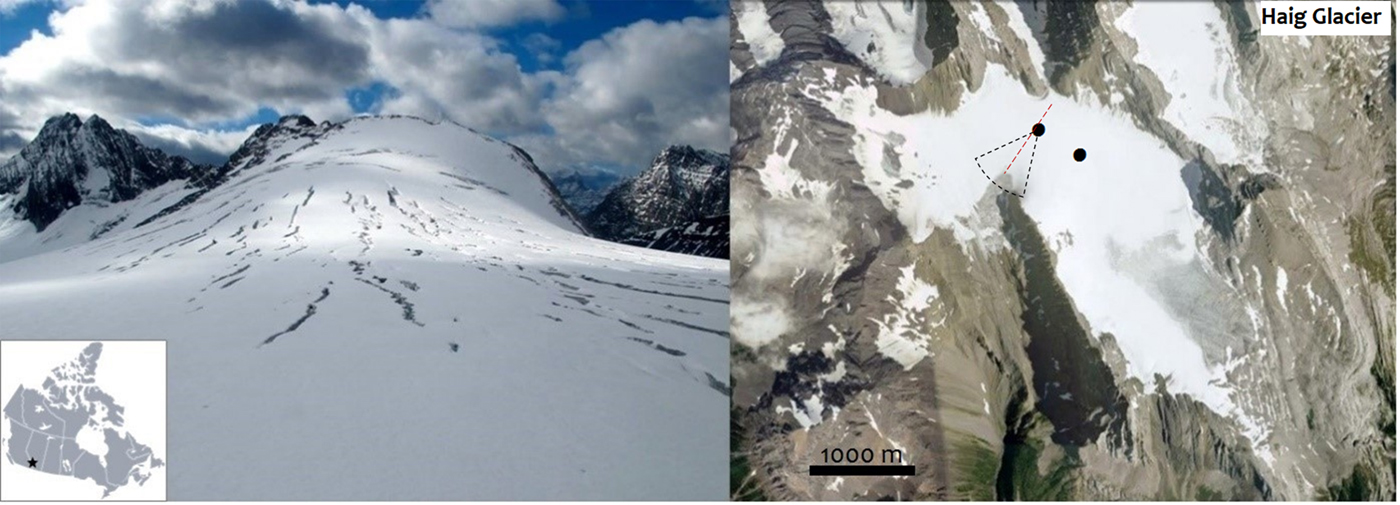
Our study investigates crevasses on Haig Glacier, a small (~3 km2) icefield that straddles the Continental Divide in the Canadian Rocky Mountains (Fig. 1). Haig Glacier flows to the southeast into the province of Alberta, with a central flowline length of 2.7 km, a mean glacier elevation of 2660 m, and elevations ranging from 2480 to 2925 m a.s.l. Haig Glacier has been a focus for glacio-climatic studies since 2001 (Marshall, Reference Marshall2014). Moist Pacific air masses deliver relatively high annual precipitation totals to the study site (Sinclair and Marshall, Reference Sinclair and Marshall2009), averaging ~1300 mm w.e., or 3.2 m of snow, across the glacier over the winter accumulation season. In situ data collected from May through September 2015 are used to drive and constrain a glaciological mass-balance model for comparison with the LiDAR data.
(Left) Field photo of Haig Glacier crevasses, September 2015 (photo credit: S. Samimi). (Right) Haig Glacier in the Canadian Rocky Mountains (Google Earth image) including locations of in situ mass-balance observation (dark circles) and approximate field of view for the left image. The red dotted line indicates the continental divide: the upper limits of the Haig Glacier catchment. Glacier ice to the west of this drains southward via an unnamed outlet glacier.
A snow survey was conducted on the glacier on 11–13 May 2015, before the onset of melt, including probing of snow depth at 33 sites and three snow pits dug to the previous summer surface, with snow-density measurements at 10-cm intervals. Measured snow depths ranged from 2.33 to 3.65 m along the glacier centerline, with a median value of 2.8 m. These observations inform the interpretation of LiDAR data for mass-balance studies, as measured snow depths and densities are needed to convert LiDAR-derived elevation changes to summer mass balance (water equivalent snow, firn and ice loss).
We do not maintain summer mass-balance measurements (an ablation stake network) at the site, but we established an automatic weather station (AWS) on the upper glacier in May 2015. The AWS logged four components of radiation, air pressure, temperature, humidity, wind speed and snow surface height at 30-min intervals. AWS data are used to drive a distributed energy and mass-balance model over the glacier, modified for local topographic shading, slope and aspect (Ebrahimi and Marshall, Reference Ebrahimi and Marshall2016). The model is seeded with initial snow depths and densities based on the winter mass-balance survey. We visited the glacier five times in summer 2015 to maintain the station, conduct spatial albedo surveys and monitor summer melt at two locations on the upper glacier (Samimi and Marshall, Reference Samimi and Marshall2017; Fig. 1b). The melt model is constrained by these albedo measurements, with free parameters (e.g. surface roughness coefficients) calibrated at the in situ observation sites.
Surface mass balance was strongly negative in 2015, driven by a warm early summer. All of the seasonal snow on the glacier melted by early August, and the upper accumulation area lost an additional 0.6 m of firn, for a total May-to-September vertical change of −4.3 ± 0.2 m recorded at our ablation stake on the upper glacier. Near the median elevation of the glacier, 2660 m, the total observed ice melt was 1.4 m. Combined with a May snowpack of 3.2 m, this gives a surface height change of −4.6 ± 0.2 m between May and September. We lack direct measurements of ice ablation at the toe of the glacier in summer 2015, so we rely on the surface energy balance model for glacier-wide summer melt estimates to compare with the LiDAR data.
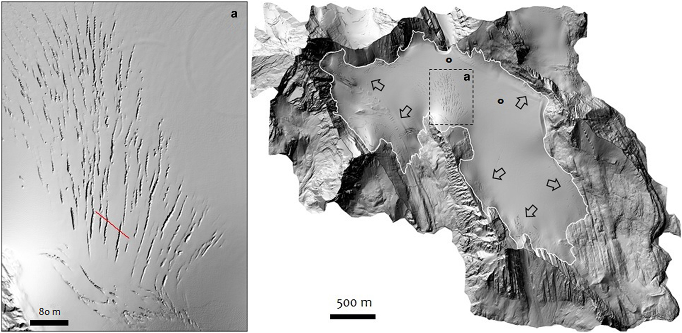
Numerous crevasses opened up on the upper glacier in August 2015, between ~2700 and 2925 m elevation. This area of the glacier lost all of its seasonal snow several times from 2001 to 2017, but many of the crevasses that appeared in August 2015 were not previously observed. Oblique imagery (Fig. 1) illustrates some of these crevasses in the upper accumulation area in mid-September 2015, with ~20 cm of fresh snow on the glacier. Crevasses that appeared in summer 2015 persist through to summer 2019. Figure 2 shows a shaded relief image of the LiDAR DEM from September 2015. Crevasses are evident in airborne LiDAR data in late-summer glacier images, when they are not snow-bridged (Fig. 2a). The April DEM in this study indicates a smooth, snow-covered surface over the entire glacier, with no visible crevasses. This is consistent with observations from spring field visits.
Shaded relief image of Haig Glacier extracted from 1-m LiDAR DEM. Arrows indicate locations with high density of crevasses. (a) Region of the glacier with intense crevassing. Red line is the transect line of Figure 5.
Methodology
The primary goals of this study are: (i) to introduce a framework for mapping and extracting the morphometry of crevasses on glacier surfaces, and (ii) to use the resulting crevasse mask as a filter for glacier studies that might be compromised by crevasse topography (i.e. due to the impact of crevasses on elevation change inferences for geodetic mass-balance calculations). To address this, we apply an ANN algorithm known as self-organizing maps (SOM) (Kohonen, Reference Kohonen2001). This algorithm is strong in outlining linear features such as crevasses. Application of SOM with suitable settings in network and input layers facilitates our image processing and crevasse analyses in glaciological studies.
LiDAR/DEM development
Airborne laser scanning LiDAR data have a sampling density of 1–2 returns per square meter and a relatively high vertical accuracy (±15 cm). LiDAR has gained widespread use as a tool to generate DEMs that are superior to DEMs from topographic maps or satellite imagery (Nelson and others, Reference Nelson, Reuter and Gessler2009). Previous studies demonstrate that LiDAR data can be successfully used to characterize linear features such as streams and their order, magnitude, width, sinuosity and channel morphology (James and others, Reference James, Watson and Hansen2007; Cavalli and others, Reference Cavalli, Tarolli, Marchi and Dalla Fontana2008; Vianello and others, Reference Vianello, Cavalli and Tarolli2009; Biron and others, Reference Biron, Choné, Buffin-Bélanger, Demers and Olsen2013). Investigations have confirmed that LiDAR data can be used to identify and track glacial crevasses (Arnold and others, Reference Arnold, Rees, Devereux and Amable2006; Jóhannesson and others, Reference Jóhannesson, Björnsson, Pálsson, Sigurðsson and Þorsteinsson2011).
We performed airborne surveys of Haig Glacier on 20 April and 12 September 2015 using a Reigl 580 laser scanner with a dedicated Applanix PosAV 910 Inertial Measurement Unit (IMU). Flight paths were 400–500 m above the glacier surface, at a flight speed of ~50 m s−1 and with a beam divergence of 0.2 mrad, yielding a beam diameter of ~0.1 m. Laser shot densities for the April and September surveys averaged 2.89 and 0.93 m−2, respectively. We processed LiDAR and flight trajectories using Applanix's PosPac Mobile Mapping Suite which yielded vertical and horizontal positional uncertainties of ±0.15 m (1σ). We generated DEMs used in this study from post-processing point cloud using LAStools (https://rapidlasso.com/lastools/) and the LAStools las2DEM algorithm on classified point clouds. This algorithm triangulates ground classified airborne laser scanning points into a triangulated irregular network from which we created 1 m DEMs using nearest neighbor interpolation. The DEMs were coregistered following the methods described in Nuth and Kääb (Reference Nuth and Kääb2011). This co-registration produced vertical errors of ±0.25 m (1σ) over areas of stable terrain. A full summary of methods pertaining to our LiDAR processing steps and the uncertainties is found in the Supplementary Material of Menounos and others (Reference Menounos2019).
Input layers for crevasse delineation in SOM
Surface crevasses on glaciers form due to brittle failure under tension as ice undergoes extension (velocity divergence) in association with flow over bedrock obstacles, lateral drag from valley walls, changing valley width or orientation, basal sliding, or drawdown of the terminus (Hargitai and Kereszturi, Reference Hargitai and Kereszturi2015). Depending on their genesis, crevasses have different depths, widths and shapes. Most crevasses have nearly vertical walls, and usually propagate downward from the surface. They can widen and deepen under continued extensional stress as well as thermal and mechanical erosion from supraglacial waters that drain into crevasses (Morawski, Reference Morawski2010; Benn and Evans, Reference Benn and Evans2014). The underlying topography and its deformability due to the load of the advancing glacier are both important in their formation zone and evolution (Morawski, Reference Morawski2010), and may cause different internal and external forms of crevasses.
Examination of strain patterns and stress regimes on glaciers through multi-temporal analysis requires a comprehensive description of crevasse morphometry. Mapping crevasses as simple linear features misses some important information that is possible to extract. High-resolution LiDAR DEMs enable the calculation of first, second and third derivatives of local land surface features, which can be used to extract a more complete 3D set of geomorphometric crevasse parameters.
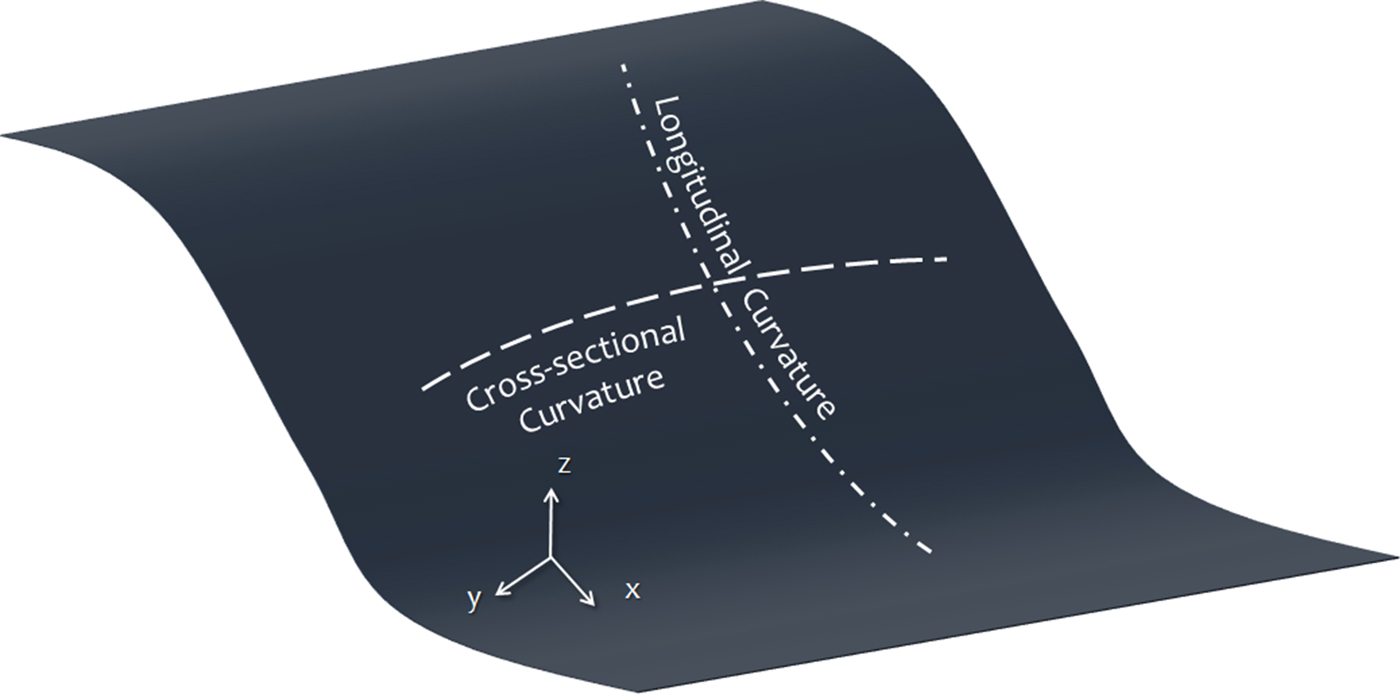
Geomorphometric parameters are topographic variables extracted from elevation models; each can be useful in defining a specific aspect of a landform or shape characteristic. More than 20 geomorphometric parameters have been introduced by different studies (e.g. Florinsky, Reference Florinsky2009; Hengel and Reuter, Reference Hengel and Reuter2008). We examine these parameters based on crevasse shapes in our study area, to select the best factors that delineate crevasses. We consider both cross-sectional (transverse) and longitudinal curvature (Fig. 3), corresponding to the planform and profile curvature of Zevenbergen and Thorne (Reference Zevenbergen and Thorne1987), respectively. Cross-sectional curvature, in the direction perpendicular to the surface slope, defines geomorphological form when surface concavities such as channels and longitudinal crevasses are detected (Wood, Reference Wood1996). Longitudinal curvature is the curvature in the down-slope direction, and helps to identify transverse crevasses. Curvature is important in the morphology of crevasses because of their iconic, relatively sharp cross-sectional profile compared with the rest of the glacier surface (Hengel and Reuter, Reference Hengel and Reuter2008; Hargitai and Kereszturi, Reference Hargitai and Kereszturi2015).
Schematic illustration of two second-order derivatives of elevation: cross-sectional and longitudinal curvatures. Cross-sectional curvature measures curvature perpendicular to the downslope direction, while longitudinal curvature measures curvature in the downslope direction.
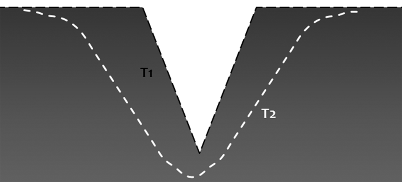
We also identify unsphericity as a factor for further analysis of these features with repeated DEMs. It is a nonnegative curvature, equal to zero on a sphere and positive outside a sphere (Hengel and Reuter, Reference Hengel and Reuter2008); it characterizes how far a surface is from a sphere, which can help in evaluating changes in crevasse rims over time (Fig. 4).
Changes in the form of rims and troughs of crevasses from aging in the crevasses with no extension or compression dynamics. This evolution can be recognized on DEMs by using the unsphericity parameter. The schematic image indicates the decrease in unsphericity (crisp and sharp edges becoming rounded) over time.
Geomorphometric parameters were examined visually to identify the ones which best exemplify crevasse morphology at our site. They have been displayed and analyzed for crevasse locations to identify parameters that define all parts of a crevasse including its sinuosity, concavity and rim sharpness and consequently its outline and anomalies on the glacier. For extracting these parameters, a local window is passed over the LiDAR DEM and the change at each point relative to surrounding points is derived by a bivariate quadratic function of the surface:

where f is the height at the central point of the window and p, q, r, s and t coefficients are partial derivatives $\left( {p = \; {\textstyle{{\partial z} \over {\partial x}}}, q = \; {\textstyle{{\partial z} \over {\partial y}}},\,\; r = \; {\textstyle{{\partial^2z} \over {\partial x^2}}},\,\; s = {\textstyle{{\partial^2z} \over {\partial x\partial y}}},\,t = \; {\textstyle{{\partial^2z} \over {\partial y^2}}}} \right).$ Parameters greater than the second order do not improve crevasse classification. The optimal kernel size for testing in the methodology has been initially identified visually, selected to give an output layer, which captures the size, orientation and location of individual crevasses.
Crevasses have linear shapes and their footprint compared with the whole study area is relatively low, so we need to use small kernel sizes for better delineation of the elements. However, to reduce high resolution DEM errors that could have significantly affect the curvature parameters of small features (Sofia and others, Reference Sofia, Pirotti and Tarolli2013), through our methodology we have identified 5 × 5 as the best kernel size for all parameters that have been used for crevasses (p, q, r, s and t: quadratic coefficients) as formulated below:
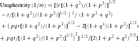
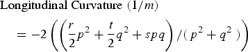
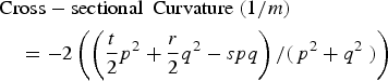
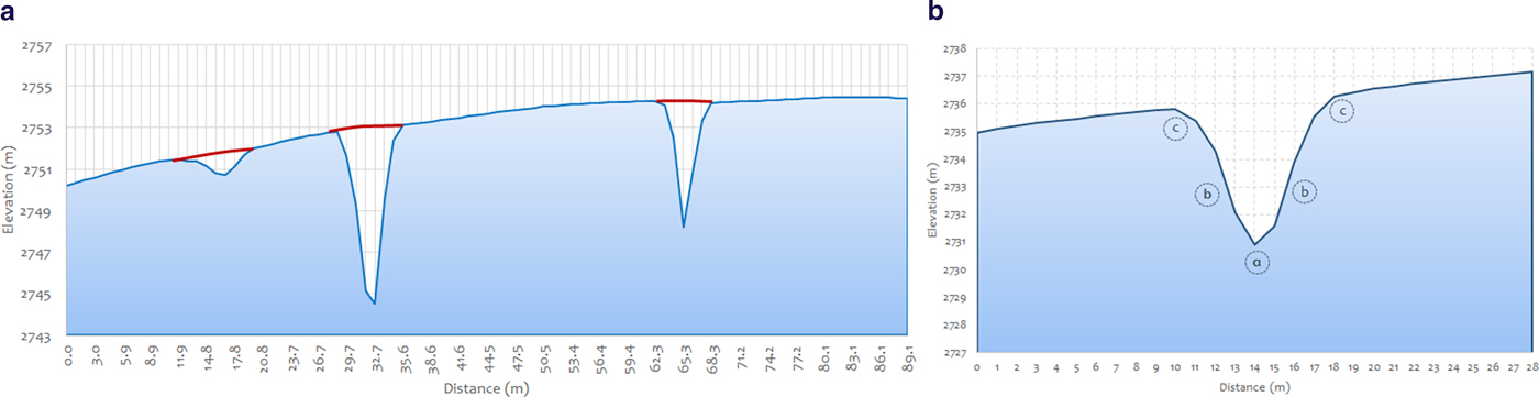
Equation (3) is from Shary (Reference Shary1995), Eqn (4) from Krcho (Reference Krcho1973) and Eqn (5) from Wood (Reference Wood1996). The length of each crevasse is the centerline length, while the width factor is defined from the middle of each feature, perpendicular to the centerline. Orientation, however, is the alignment of the straight line distance between two ends of the feature. We calculate minimum crevasse depth by removing identified crevasses from the DEM and estimating the planar surface through inverse distance weighted (IDW) interpolation using the crevasse edge points. This is a common method in geoscience and is an accurate interpolator for DEM generation with LiDAR data (Su and Bork, Reference Su and Bork2006; Ashraf and others, Reference Ashraf, Hur and Park2017). The lowest point in each crevasse is then found by subtracting the crevasse elevation model and the planar surface that replaces it, giving the deepest detected part of each crevasse in our data (Fig. 5a). These are minimum depths because the LiDAR may not have detected the deepest part of each crevasse, but could be returning an internal reflection from the sides. For accuracy assessment of the results, 50 randomly selected crevasses from different locations of the glacier have been digitized and their extent properties have been extracted manually.
Self-organizing map (SOM) application
ANN algorithms have been widely applied in a variety of different scientific disciplines. Sample applications in geoscience and remote-sensing studies include image classification (Foroutan and others, Reference Foroutan, Kompanizare and Ehsani2013; Maggiori and others, Reference Maggiori, Tarabalka, Charpiat and Alliez2017), crestline mapping (Foroutan and Zimbelman, Reference Foroutan and Zimbelman2017), river flow prediction (Karunanithi and others, Reference Karunanithi, Grenney, Whitley and Bovee1994; Akhtar and others, Reference Akhtar, Corzo, Van Andel and Jonoski2009), hydrological modeling (Dawson and others, Reference Dawson and Wilby2001) and estimation of glacier ice thickness from terrain morphometry (Clarke and others, Reference Clarke, Berthier, Schoof and Jarosch2009; Quiroga and others, Reference Quiroga2013). These networks consist of layers of neurons, which are inter-connected and act as processing units. Each output layer neuron is connected to all neurons in the input layer by synaptic weights (weight vectors). By adjusting the weights of neurons, preferred classification from the network can be obtained.
In general, ANNs consist of layers of neurons which are inter-connected and act as processing units. The SOM or Kohonen network, after its inventor (1982), is one of the most extensively used unsupervised ANN algorithms (Kohonen, Reference Kohonen2001). It executes a characteristic nonlinear projection from high-dimensional space onto a low-dimensional array of neurons, which is useful for identifying and visualizing complex and underlying patterns from small to large datasets. The SOM is a competitive learning algorithm, and competes to give the best representation of the input data during the learning process. SOM has a topology-preserving characteristic (Kohonen, Reference Kohonen2001), meaning that vectors that are close in the input space will be mapped to units that are close in the output map (Vesanto and others, Reference Vesanto, Himberg, Alhoniemi and Parhankangas2000; Bação and others, Reference Bação, Lobo and Painho2005), which is a unique feature. Unlike other ANN algorithms, SOM uses a neighborhood function for identifying the topological properties (geomorphometry here) in the inputs. In addition, unlike with other multivariate methods, with SOM, there is no need for a priori interpolation when data are missing (Richardson and others, Reference Richardson, Risien and Shillington2003).
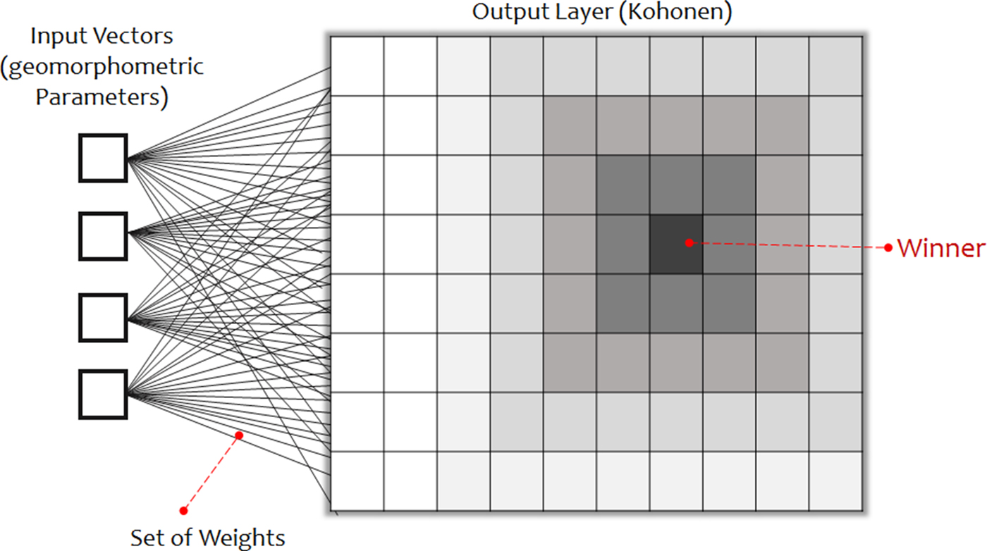
The SOM architecture classically contains two layers. Apart from the Input layer, SOM has an output layer (map) of nodes (known as neurons) with initial random weights (random images on each of the nodes here). During what is termed the ‘training step’ of SOM, which is an iterative process, input data (geomorphometric layers here) are consecutively presented to the output map. Through this learning procedure, input vectors that have been introduced to the map and the distance from each weight to the sample vector are calculated by running through all the weight vectors. The node in the output map (with its initial random weight) with the minimum Euclidean distance between itself and the input vector is then identified and updated. This node is called the ‘winner’ node or best-matching unit (BMU), and becomes the center. Its neighbors will be updated based on their relative distances to BMU (Fig. 6).The training procedure is formulated in Eqn (5). An input vector is characterized by the vector x = {x 1, x 2,…, x n}, where n is the number of input variables (three geomorphometric parameters here: unsphericity, longitudinal curvature and cross-sectional curvature). The initialized weight vectors connect m × n neurons, so the winner is:

where ‖ ‖ is the Euclidean distance measure, x(t) is the input vector and w i(t) is the synaptic weight of neuron connecting output neuron to the input neuron i at iteration t. Selecting the best-input parameters is considered a pre-processing step in this study, as discussed earlier.
(a) Cross-sectional profile of three crevasses in the LiDAR data (interpolation line in Figure 2). The red line indicates the interpolated surface from an IDW interpolation technique. Subtraction of the measured elevation from the IDW surface for each crevasse gives us the estimated minimum depth of each feature. We use the interpolation surface to filter out the effect of crevasses in calculation of elevation differences on the glacier (i.e. from repeat imagery). (b) Cross-sectional profile of a crevasse in Haig Glacier identified by cross-sectional and longitudinal curvature parameters through ANN methods. (a) Identified as the deepest part of the crevasse, with negative values in both parameters; (b) crevasse walls with opposite signs in both parameters and (c) the rim of the crevasse, with positive signs for both parameters.
Schematic illustration of the SOM architecture, consisting of input and output layers and weight vectors that connect these two layers. Different gray tones in the SOM layer indicate the degree of the tuning in neighbor neurons, based on their distance to the winner or best matching unit.
Neighborhood is an important concept in SOM, because the weight vector of the winner and output neurons within a neighborhood radius γ of the winner are adjusted in the direction of the input vector as:

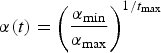
where ω i(t + 1) is the adjusted weight and α(t) is the learning rate at iteration t. The weights of those neurons outside the neighborhood remain unadjusted. Within the neighborhood nearer neighbors, receive more training, weight adjustment, than farther neurons (Fig. 6). This competitive learning and lateral interaction stage is known as coarse-tuning. During the coarse-tuning stage the learning rate declines gradually from an initial learning rate (α max) to a final learning rate (α min), after a total number of iterations (epochs) (t max):
Repeating this process, thus decreases the radius of the neighborhood (γ) gradually during the coarse-tuning stage:
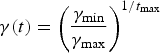
It is usually preferred to start with a large initial neighborhood radius, which decreases until the weight of just the winning neuron is attuned in the output layer. This is called the ‘mapping step’. Finally, the output map will become self-structurally shaped by learning, which leads to a topology (regional organizations of neurons) in the output map, and is the fundamental organization of neuron weights that represent separate classes in the input layer. For detecting the existing patterns, a map of the average distance of a neuron to its neighbors can be visualized in the U matrix. This map itself can be organized into different clusters, with a K-means algorithm used in this study. Ultimately, after the SOM is performed, a classified 2-D image is reconstructed from node weights. The value of each pixel in the original map is substituted by the value of its corresponding neuron weights (which is now in a class) and the desired class (crevasses here) on the initial image extent will be detected. SOM structure can be coded in any programing software or conducted in ANN modules of professional software with precise setting options, particularly image processing packages. However, finding the best setting for extracting the target features is challenging, and several settings must be tested and be programed. The SOM in this study was performed in the MATLAB environment.
Considering the linear shape of the crevasses and their small area compared with that of the much larger host glacier, we are technically taking advantage of one of the shortcomings of the SOM algorithm, known as the magnification factor (Cottrell and others, Reference Cottrell, Fort and Pagès1998), to identify linear features such as crevasses. The factor can be defined as the tendency of SOM to overestimate low probability areas, a factor that may not be found in other ANN methods. In this study, the procedure starts on one side, geomorphometry, with selecting the best parameters as inputs. Statistical parameters such as optimum index factor (Chavez and others, Reference Chavez, Berlin and Sowers1982) can be used for this selection. However, in this study, as discussed previously, we carefully chose the best parameters based on our understanding about crevasse geometry. The kernel size for producing the selected parameters from a DEM is considered a part of the SOM configuration in this study. After the parameters are built and selected, each is normalized with a logistic transformation between zero and one.
Assignment of appropriate settings and learning parameters is the most-important step in efficiently extracting a specific feature using SOM in the detail that is needed. The most important control parameters are: (1) the output layer neuron size, which has a direct correlation with the level of details that would be expected for the classification. For the fully delineation of the target feature outline, the optimum size needs to be identified. Initial neighborhood radius also depends on the output layer neuron size. (2) The number of iterations, which is the number of times that the input data will be presented to the map. All these criteria have been selected by trial and error, and the results compared by evaluating the quality of SOM performance using the quantization error (QE) as the criterion:
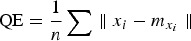
where n is the number of inputs, x i is the input and $m_{x_i}$ is the BMU. The error describes the neural map fitting to input data, which means Euclidian distance between data vectors and BMU, and the smallest average QE denotes the optimal solution. For example, the necessary number of iterations can be determined by monitoring QE; once it stops decreasing and remains constant, no more are needed. On the other hand, small output layer neuron size may not properly identify the target features and large output size might miss-classify the targets, so for all control parameters, it is critical to identify the optimal and efficient values.
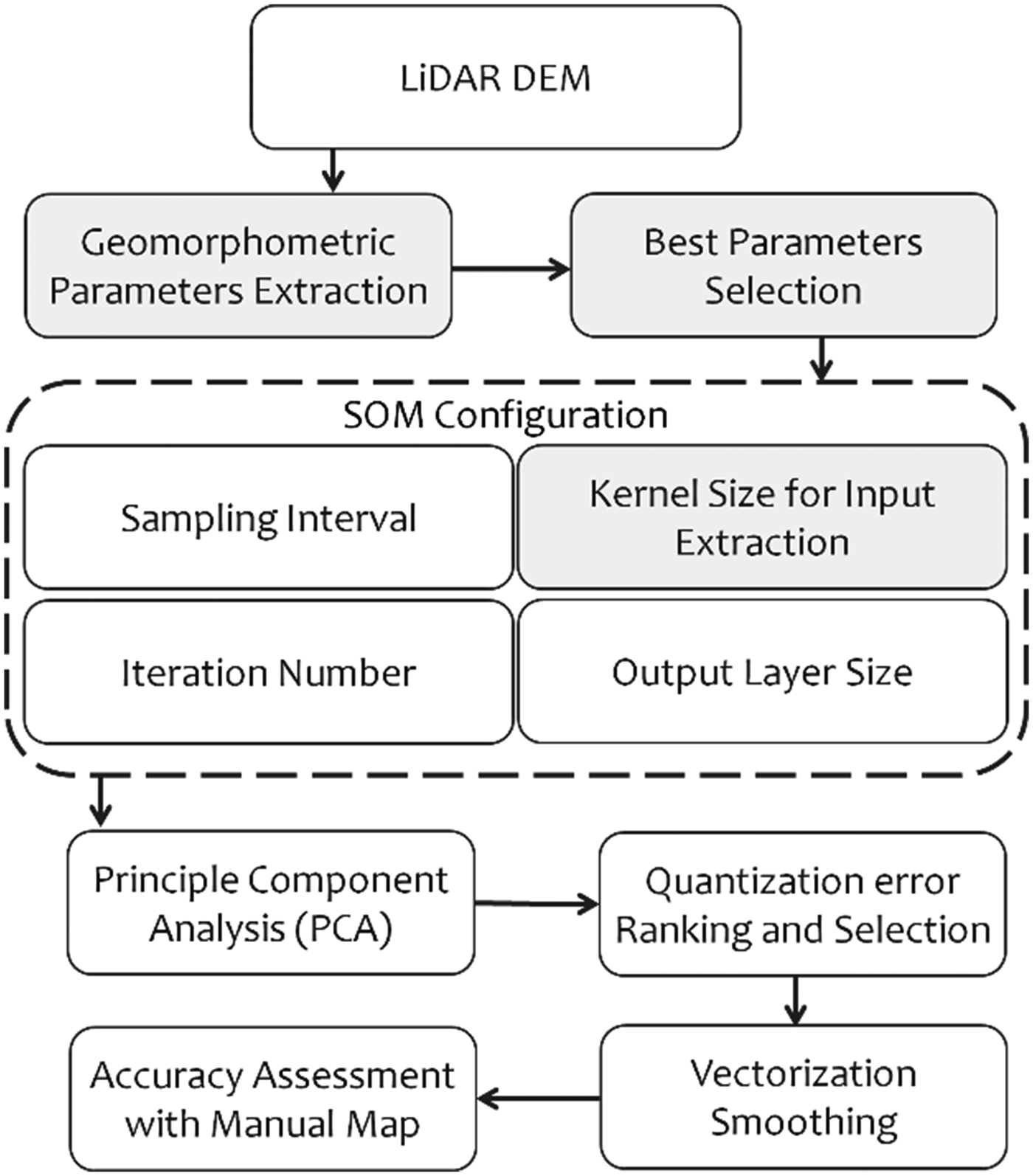
For this study, the random initialization of weights has been used and the initial neighborhood radius adjusted to be equal to the output layer's diagonal size, which is the maximum possible. To identify the optimal map with the best setting and configuration, several sets of configurations have been applied using different configuration parameters. This approach resulted in ~800 classification results, from which repeated and redundant final maps have been removed using principal component analysis as the identification procedure using the methodology introduced by Jolliffe (Reference Jolliffe1972). The final resulting maps have been narrowed down to 20 classified images with the least QE value. Ultimately, the selected maps were vectorized (nonsimplified) and smoothed by Polynomial Approximation with Exponential Kernel in Arcmap before accuracy assessment with a precise manually digitized map. The extent of the manually extracted crevasses, as the reference map, have been examined and compared with the SOM results, in terms of average areas of overlap and outlier. Finally, the most accurate crevasse map has been selected (Fig. 7). In simple terms, the impacts and quality of different setting parameters have been analyzed to gain the best result. Because of the shape of crevasses in this study and precise parameter selection procedure, identifying the target class is straightforward by manual reclassification, but labeling can also be conducted automatically by using unsupervised statistically weight-based labeling procedure (van Heerden and Engelbrecht, Reference van Heerden and Engelbrecht2013). The final crevasse binary raster map has been converted to a vector file and smoothed. Their dimensions were then measured using the final vector image. These procedures can all be coded in a single file, or one can use modules from different software for each step.
The flowchart indicates the methodology that has been applied in this study to find the best SOM configuration.
Results and discussion
The input dataset and final maps indicate that crevasses can be identified and mapped by this methodology based on different parts of the features. As an example, Figure 7b illustrates the cross-profile of a typical crevasse that has been defined by its cross-sectional and longitudinal curvatures. The ultimate SOM setting for crevasse extraction from the LiDAR DEM of 1-m resolution has been identified as ~2.5 million iterations with an 80 × 80 output layer neuron, with one unit interval in columns and rows of the network, which gives us a QE of ~0.0095. One-meter resolution is a suitable pixel size for detailed study of the larger crevasse features, which are tens of meters in length, but some small cracks may not be detected in the LiDAR data or captured in the DEM. The resulting crevasse distribution map (Fig. 8a) demonstrates the ability of this methodology to extract crevasses of different sizes and orientations. Accuracy assessment and comparison of results with manual data indicate a 93.7% correlation between manually- and automatically-classified data. Errors are mostly close to rock walls, with high topographic differences, and in the high-density crevasse locations with very close and crossed crevasses, that could result in uncertainty in detecting individual crevasses (Fig. 8b). This result cannot be obtained using optical images with diversely-oriented crevasses, because they are affected by illumination conditions based on their angle. Crevasse orientations and densities differ across the glacier, with the highest crevasse density on the glacier in September 2015 being ~20 counts per 10 000 m2.
(a) Rose diagram (left bottom) and map of 1048 crevasses detected by the SOM method on Haig Glacier, with diverse orientation. (b) Crevasse density map (unit: number in square kilometer). Circles indicate locations with high error, which are mostly close to rock falls. Errors are particularly in the width of the crevasses, which is due to very close or crossed crevasses.
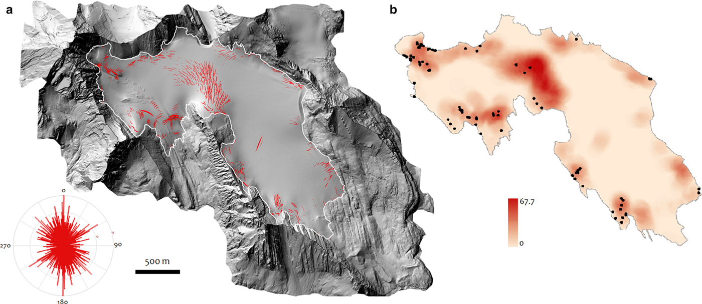
Many transverse linear crevasses exist in the north-central area of the glacier, a steeply sloped surface that promotes strong longitudinal extension (Fig. 8a). Bergschrunds are identified at the head of the glacier proximal to the ice/bedrock interface, transverse to the main flow. Lateral or marginal crevasses along the flanks of the glacier are oriented in the downslope direction. Lateral crevasses are probably associated with extensional lateral shear within the glacier, caused by friction between the flowing ice and the side walls of the valley. Arcuate crevassing here reflects local ice extension combined with lateral drag. The diversity of crevasses indicates the importance of both longitudinal and lateral stress gradients in different parts of the glacier.
Crevasse morphology
SOM results identified 1048 individual crevasses, with intersecting crevasses identified and separated based on their primary orientation. Crevasses on Haig Glacier have different sizes and range from <1 m to ~2 m in width, 3–289 m in length and between 1 and 18 m in depth (Table 1). The population of crevasses detected with our algorithm has a mean length and width of 35.6 and 0.56 m, and a mean minimum depth of 1.85 m. Considering our measurement precision of ~2 samples per m2, crevasse length distribution will be reasonably accurate, but we do not resolve crevasse widths reliably. Similarly, depth inferences are minimum estimates, since most crevasse reflections will come from the sidewall rather than the bottom of a crevasse.
Crevasse depth, width and length range (m) extracted from the SOM methodology, which shows the general overview of the crevasse dimensions detected by the LiDAR survey on Haig Glacier

Covariance of crevasse width, length, depth and local slope indicate a moderate correlation between width and depth, but no strong relation exists between length and the other dimensions. The widest and deepest crevasses are located close to the rock walls, particularly in the northwest part of the glacier. These locations also have the largest errors in extracted widths, due to closely spaced and crossed crevasses which might be captured as wider crevasses. Since crevasse presence more than doubles the absorption of solar radiation and ice ablation (Pfeffer and Bretherton, Reference Pfeffer and Bretherton1987), crevasse morphology and aspect could warrant consideration in surface ablation calculations.
Geodetic surface differences
The final map can be used to explicitly consider crevasses when calculating elevation differences on a glacier surface. Differences for repeat altimetry are used to measure snow accumulation, snow and ice melt, and glacier elevation changes due to ice motion, but mean differences may be biased in association with LiDAR signals that penetrate crevasses. Biases are greater if one of the DEM surfaces corresponds to snow-covered conditions, where crevasses are not visible. In this case, late-summer LiDAR returns that reflect from inside crevasses can appear as exaggerated vertical change (values exceeding 15 m in our data), presenting a systematic negative bias in geodetic mass-balance measurements: an overestimate of summer surface lowering.
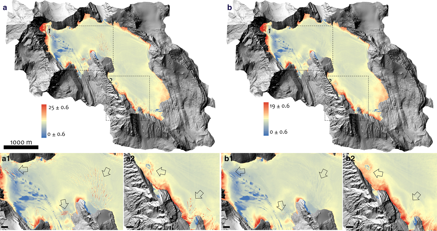
Figure 9 shows the April–September difference maps with and without the crevasse filter. Visual differences between these plots are difficult to discern, but the distribution of elevation changes is modified when the crevasses are masked out. Figure 10a plots the histogram of elevation difference values with and without the crevasse mask. The mean difference on the glacier (±1σ) for all glacier pixels on the raw, co-registered DEMs (April–September) is Δh L = −5.48 ± 0.93 m. After crevasse removal with the ANN filter, this equals −5.02 ± 0.92 m: an adjustment of ~9%.
Left: Raw (uncorrected) elevation difference map of Haig Glacier from 20th April to 12th September 2015. Warmer colors indicate crevassed regions in the map which can emphasize the importance of their existence in calculations (boxes). Right: Corrected data by using the SOM method. Zoom-in bottom images highlight these differences (scale bar = 100 m). Arrows indicate large crevasses that are present in uncorrected elevation differences (right) and have been removed in corrected data (left).
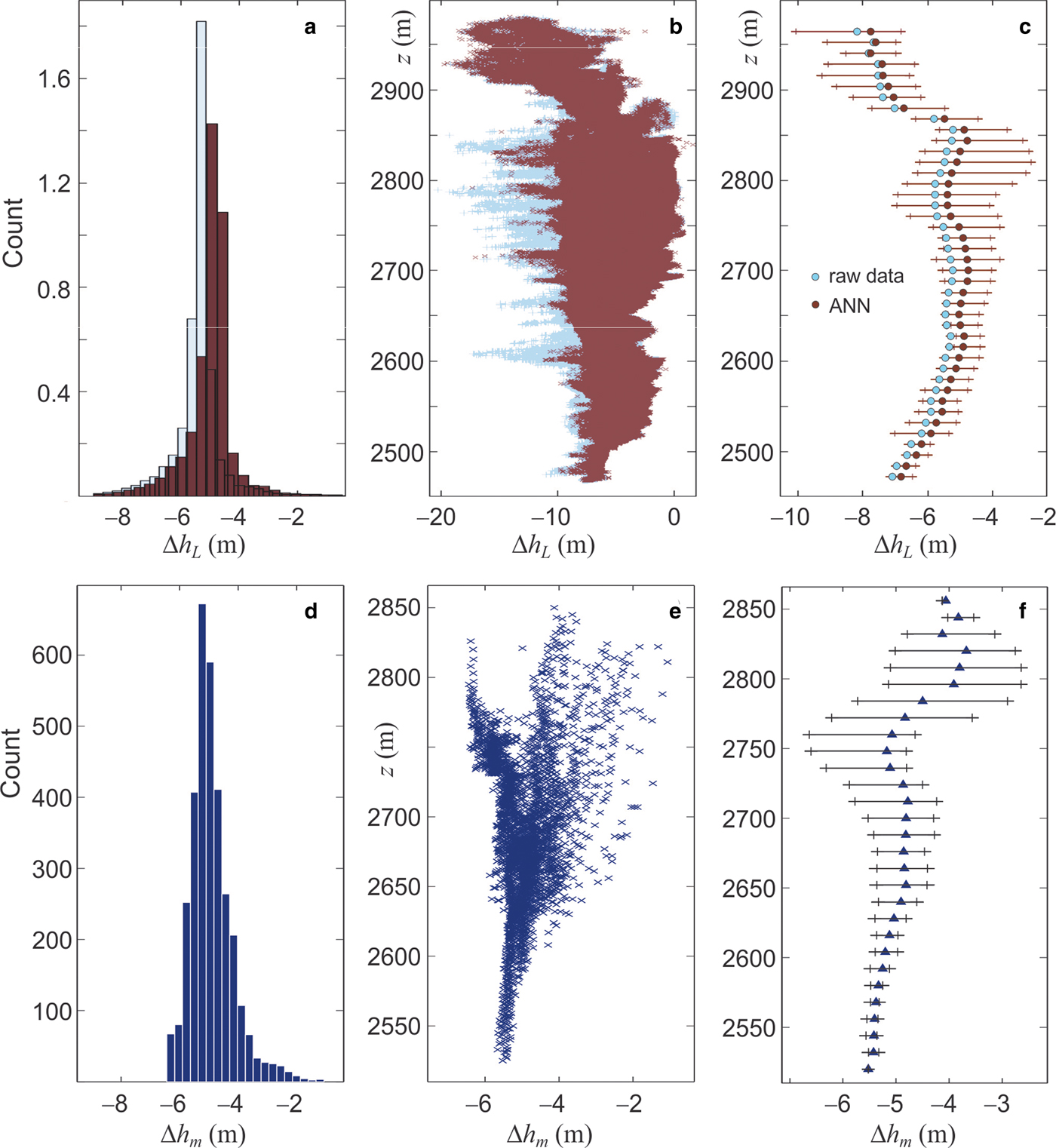
Comparison of surface elevation change in summer 2015 as measured by the LiDAR surveys (top panels) vs glaciological observations and modeling (bottom panels). The top panels show the raw LiDAR data (light blue) and ANN-filtered data with crevasse-filling (brown). (a, d) Distribution of elevation changes. (b, e) Elevation change as a function of elevation for all points. (c, f) Mean elevation change in 12-m elevation bands (circles, triangles). The ranges in these plots indicate the median elevation change ±1σ for each elevation band; ~67% of points fall within this range of elevation change.
Based on ground control sites, the estimated (1 − σ) vertical accuracy of individual LiDAR point measurements is σ z = 0.1 m. The spatial autocorrelation length scale in the LiDAR data are estimated to be ρ = 300 m (Menounos and others, Reference Menounos2019), or it has been estimated at ρ = 500 m in prior work (Nuth and Kaab, Reference Nuth and Kääb2011; Brun and others, Reference Brun, Berthier, Wagnon, Kääb and Treichler2017). Spatial autocorrelation reduces the effective sample size for calculating the difference of means (i.e. the elevation change). Following Rolstad and others (Reference Rolstad, Haug and Denby2009, eqn 14), the effects of spatial autocorrelation on the elevation change error are calculated from σ e = σ z(πρ 2/5A)1/2, for glacier area A. Using the more conservative estimate ρ = 500 m along with A = 2.8 km2, σ e = 0.024 m and the 0.46-m difference between the two estimates of mean surface elevation change is statistically significant.
Surface elevation change is plotted as a function of elevation in Figures 10b and 10c. The relation between elevation and elevation change is weak relative to the variance at a given elevation, at odds with the expectation of greater thinning at lower elevations. In part, this is because the LiDAR-inferred elevation difference, Δh L, includes changes due to both surface mass balance (summer ablation) and vertical glacier motion. Subsidence on the upper glacier and emergence on the lower glacier oppose the elevation dependence of the surface mass-balance signal. The deeper snowpack and firn on the upper glacier also result in a lower average density for the mass that ablates at higher elevations. Hence, vertical differences are greater for a given amount of water-equivalent melt (i.e. melt energy), further weakening the elevation gradient in glacier thinning.
Below 2850 m, the expected trend of decreased elevation change with higher elevation is evident in Figure 10c, which plots the mean elevation change vs elevation. This can be thought of as a centerline elevation profile, with LiDAR points averaged in 12-m elevation bins. Horizontal lines in Figure 10c indicate the median elevation change ± 1 std dev. in each elevation bin, and is only plotted for the ANN results. This encompasses ~67% of points (elevation changes roughly approximate a normal distribution). The ANN crevasse-filling procedure decreases the estimated elevation change by a relatively constant amount (~0.5 m) through the middle of the glacier, with lower differences at the lowest and highest elevations.
Surface drawdown in excess of 10 m is inferred at the highest elevations in Figures 10b, c (above ~2850 m a.s.l.). This is likely associated with LiDAR reflections from bergschrunds and ice rifts at the glacier headwall, which open up over the summer melt season. This is visible in Figure 9, which indicates large elevation changes at the glacier margins. Large changes along the terminus margins represent a genuine signal: high ablation combined with terminal retreat of several meters over the summer. For the lateral margins and the steep glacier headwall, the LiDAR is picking up bergschrunds adjacent to the valley walls and rifts that propagate downslope from this. The crevasse mapping technique does not appear to completely capture the morphology of these features. These regions are also subject to heavy winter snow-loading from sloughing/avalanches from the steep rockwalls. Avalanche deposits are not accounted for in our snow survey, but may contribute to the large elevation changes inferred from the LiDAR difference maps at the glacier headwall.
Another notable contrast is that the range of modeled Δh m is narrower than that of Δh L, with a std dev. about half of the observed (LiDAR) signal. The variability in geodetic and surface mass-balance signals should be comparable, as spatial variations associated with vertical ice motion (ice dynamics) will be smoothed relative to local surface mass-balance effects. Some of the difference in the variance may be due to the LiDAR-inferred glacier surface change picking up residual crevasses and bergschrunds that our algorithm failed to detect and remove. The mass-balance model also lacks some of the spatial complexity and inhomogeneity that is present in the real world, e.g. small-scale variations in surface albedo, snow depth, and microclimate. In this respect, the LiDAR data will give a better representation of the spatial variability.
The distribution of LiDAR-inferred ice surface elevation changes (Δh L) can be compared with the predictions of a distributed surface energy and mass-balance model. The model is seeded with initial snow depths and densities based on the winter mass-balance survey. Summer ablation is calculated from the surface energy balance, using in situ AWS data distributed over the glacier, modified for local topographic shading, slope and aspect (Ebrahimi and Marshall, Reference Ebrahimi and Marshall2016). The model has a horizontal resolution of 23 m × 36 m, giving 3621 gridcells over the glacier. While coarse compared with the LiDAR data, this provides an estimate of the spatial pattern of surface elevation changes associated with the surface mass balance, Δh m. Results are plotted in Figures 10d–f, while Figure 11 provides a direct comparison of the LiDAR data and the glaciological model. Elevations are restricted to 2510–2866 m for this comparison, the elevation range of Haig Glacier; the LiDAR data (Figs 10a–10c) include numerous additional datapoints from adjacent glacial systems, which are not part of the Haig Glacier catchment or model (see Fig. 1).
Mean surface elevation change vs elevation on Haig Glacier over summer 2015, calculated in 12-m elevation bands for the raw LiDAR data (light blue diamonds), with the ANN crevasse-filtered (brown circles), and from the glaciological model (dark blue triangles). Data are plotted for the range of elevations of Haig Glacier (2510–2866 m).
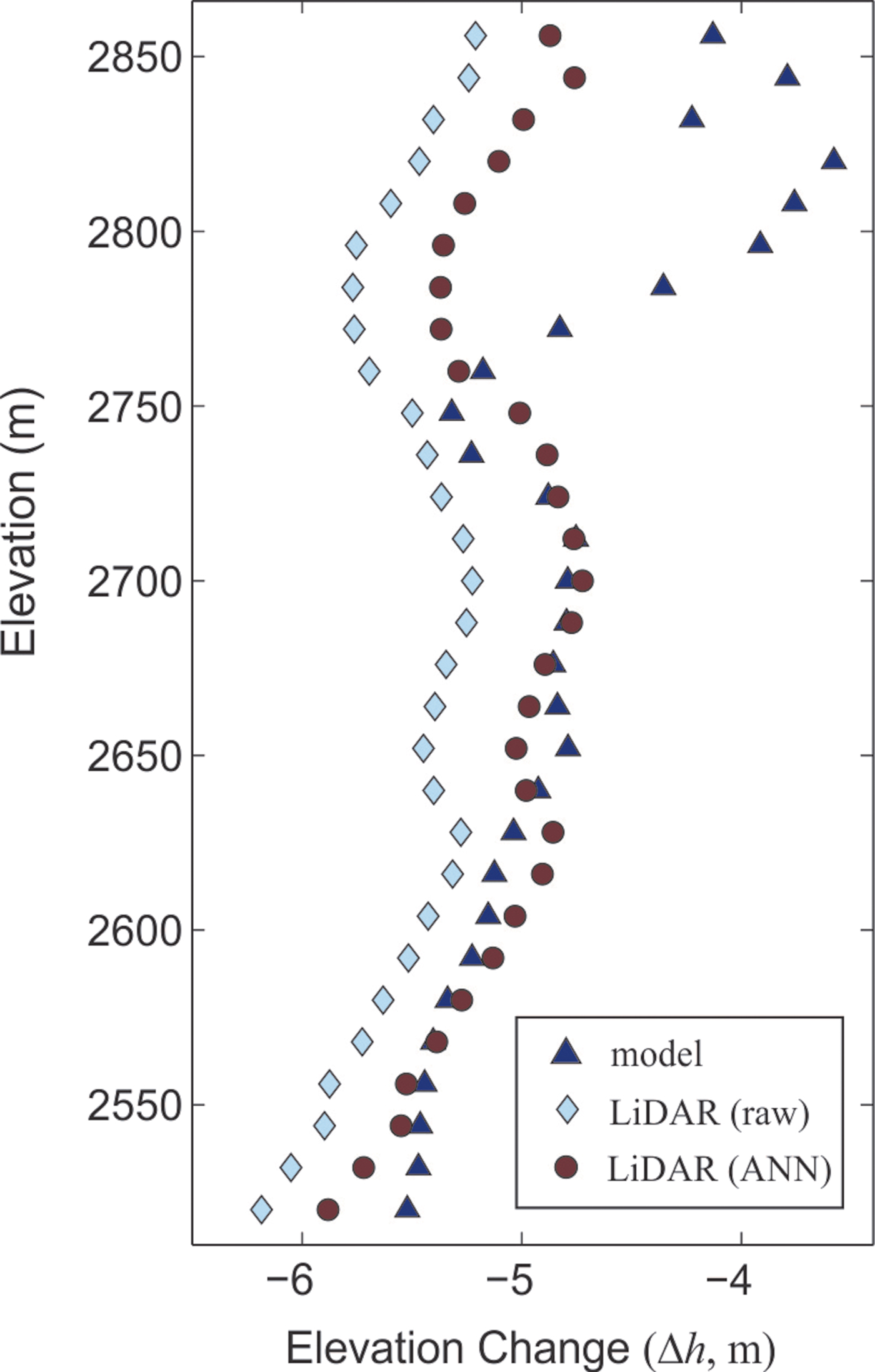
The winter 2015 snowpack ranged from 2.4 to 3.6 m deep along the glacier centerline (960–1450 mm w.e.), with a mean specific winter mass balance of B w = 1220 mm w.e. The modeled summer mass balance is B s = −3030 mm w.e., giving a net balance of B n = −1810 mm w.e. This includes an estimated 40 mm w.e. of summer snowfall. Expressed as surface height, adjusting for the densities of snow, firn and ice, the average modeled height change (± 1σ) is Δh m = −4.92 ± 0.72 m, with a range from −6.44 to −1.07 m. There is a large degree of consistency between the model with the LiDAR-inferred elevation changes, but there are also some interesting differences. In both cases, more than 80% of the points fall in the range Δh = −6 to −4 m (Figs 10a, d). The mean elevation change in the model is within 0.1 m (2%) of the crevasse-filtered LiDAR results, and none of our simulations provided a good fit with the raw LIDAR data.
The model appears to underestimate ablation near the glacier terminus, but in general the ANN results and the glaciological model are in good accord below ~2760 m (Fig. 11). The model exhibits less variability than the LiDAR data, which is to be expected given the lower resolution and simplifications inherent in the model (e.g. a single albedo for glacier ice). There is strong divergence between the model and the LiDAR data above ~2760 m though, with modeled thinning of ~4 m on the upper glacier compared with surface drawdowns of ~5 m in the ANN-filtered LiDAR data. The LiDAR data includes vertical changes associated with both summer melt and ice motion; these data therefore suggest that there may be a submergence signal on the order of 1 m over the summer, corresponding to a submergence velocity of ~2.5 m a−1. However, we do not see an analogous emergence velocity signal on the lower glacier. The surface energy balance model may underestimate the ice melt on the lower glacier. This could be caused by energy balance processes that are not included in the model such as heat advection from exposed rock near the glacier terminus or low ice albedo (values below 0.2) on the lower glacier, where impurities have a higher concentration.
Conclusions
An automatic methodology for mapping and geometric analysis of crevasses based on SOM is described in the current study. The methodology successfully extracts the topography of more than 1000 crevasses on a small mountain glacier in the Canadian Rocky Mountains. Comparing the resulting map with 50 manually-extracted crevasses from the same data indicates an accuracy of 94% for those crevasses that are detected by the LiDAR. Additional small crevasses may not be seen in the imagery. This result indicates the power of using SOM with simple geomorphometric factors, cross-sectional and longitudinal curvatures, in extracting small features such as crevasses. This study also highlights the ability of LiDAR elevation data to catch small surface irregularities and the potential to exploit this in glacier studies. The extracted crevasse fields indicate diverse stress configurations on Haig Glacier, which can be related to ice flow fields. Movement of surface crevasses as well as their geometric changes over time could also be observed through repeat LiDAR DEMs. In addition, applying unsphericity curvatures can give us more information about crevasse rim changes, which can add a new aspect to crevasse transformation studies in remote sensing.
Moderate- to large-scale glacier crevasses are penetrated by airborne LiDAR when there is no snow cover on the glacier, giving reflections from several meters below the surface of the glacier. This reflection can cause elevations of the LiDAR-derived DEM to be too low and may causes errors in differences that are used for geodetic mass-balance monitoring. Automatic detection, masking and removal of crevasses can be carried out to give a more accurate surface elevation of the glacier as well as provide maps of crevasse distribution that can be used for analysis of glacier stress and flow regimes.
The crevasse-removal filter reduces the LiDAR-inferred average glacier thinning from 5.48 to 5.02 m at Haig Glacier in summer 2015. In essence, false returns from crevasses produce a 0.46 m (9%) difference of glacier elevation change compared with the ANN crevasse-filtered results. The mapping technique and crevasse-removal algorithms should be considered in calculation of glacier-wide elevation differences for glacier change analysis. Our methodology, or alternative crevasse-filtering techniques, may improve the accuracy of geodetic mass-balance studies in glaciology, but our approach would also require additional testing with a richer dataset that spans multiple glaciers and multiple years. Geodetic balance calculation for two end-of-summer DEMs without crevasse removal would introduce less bias than differencing an end-of-winter and end-of-summer DEMs.
In some situations, DEMs that include crevasses may be desirable, as a truer representation of surface topography; in essence, crevasses are void spaces in the glacier, and estimates of glacier volume (hence volume change) could treat them as such. In this case, the crevasse detection algorithm could be combined with assumptions about crevasse shape and depth to estimate the void volume that is associated with crevasses. This is only possible in late summer, however, when crevasses are not snow-bridged and can be detected. In our study the magnitude of this bias is probably also a maximum value since the 2015 melt season was exceptional and so would tend to maximize the exposure and widening of crevasses due to melt along their walls. We plan to study repeat data from Haig Glacier in future years through the introduced ANN methodology and to produce detailed change detection maps, which will give us additional information about the evolution of the spatial snow accumulation, melt and elevation change patterns on the glacier. LiDAR-derived crevasse maps also have the potential to convey more information about the glacier history and flow conditions.
Acknowledgements
We thank the Natural Sciences and Engineering Research Council (NSERC) of Canada, the Canada Research Chairs Program and the Canada Foundation for Innovation for supporting this research. M.F. was supported by a graduate research fellowship from NSERC and R. Vogt acquired and helped process the LiDAR data. Two anonymous reviewers provided insightful comments that significantly improved our manuscript. We also acknowledge Scientific Editor Bea Csatho for her invaluable efforts in improving this manuscript. The code from this analysis is available from M.F. on request.


 Open access

