

1. INTRODUCTION
Variations in glacier basal motion induce ice surface speedups on diurnal (e.g., Iken and Bindschadler, Reference Iken and Bindschadler1986), multi-day (e.g., Bartholomaus and others, Reference Bartholomaus, Anderson and Anderson2008; Das and others, Reference Das2008), seasonal (e.g., Mair and others, Reference Mair2003) and multi-annual (e.g., Kamb and others, Reference Kamb1985) timescales. The realization that velocity can fluctuate on seasonal timescales in some regions of the Greenland ice sheet (GrIS; Zwally and others, Reference Zwally2002) suggested that changes in basal motion could allow the ice sheets can respond more quickly to climate warming than previously expected (Parizek and Alley, Reference Parizek and Alley2004). In addition, basal sliding is required for a glacier to erode its bed (e.g., Hallet, Reference Hallet1979; Iverson, Reference Iverson1991), making understanding of this process important for modeling the evolution of both polar and alpine landscapes over geologic timescales (e.g., Harbor, Reference Harbor1992; MacGregor and others, Reference MacGregor, Anderson, Anderson and Waddington2000; Anderson and others, Reference Anderson, Molnar and Kessler2006; Herman and others, Reference Herman, Beaud, Champagnac, Lemieux and Sternai2011b; Beaud and others, Reference Beaud, Flowers and Pimentel2014).
Variations in glacier surface velocity have been observed for decades using optical surveying of displacement stakes (e.g. Iken and Bindschadler, Reference Iken and Bindschadler1986) and, more recently, through on-glacier GPS monuments (e.g. Anderson and others, Reference Anderson2004; Flowers and others, Reference Flowers, Roux, Pimentel and Schoof2011; Tedstone and others, Reference Tedstone2013; Kehrl and others, Reference Kehrl, Horgan, Anderson, Dadic and Mackintosh2015). The logistics and expense associated with installing, maintaining and resurveying monuments has meant on-glacier GPS and displacement stakes are typically sparse. Therefore, previous studies on individual glaciers have often focused more on temporal variation than spatial variations in glacier motion. Where spatial analyses are presented, they are often along a glacier flowline and resolve only along-flow velocity patterns (Anderson and others, Reference Anderson2004; Bartholomaus and others, Reference Bartholomaus, Anderson and Anderson2008; Sole and others, Reference Sole2011). However, several studies do investigate spatial patterns in basal motion in both planview dimensions (Harbor and others, Reference Harbor1997; Mair and others, Reference Mair, Nienow, Willis and Sharp2001; Nienow and others, Reference Nienow2005; Riesen and others, Reference Riesen, Sugiyama and Funk2010). These studies have highlighted the limitations of attributing basal sliding to solely local variables such as subglacial water pressure at a point, local basal traction, or the locally defined driving stress.
Satellite remote sensing has facilitated the measurement of spatially distributed glacier velocity fields using optical image cross-correlation (Scambos and others, Reference Scambos1992), but studies have been limited by relatively coarse spatial and temporal image resolution (e.g. Scherler and others, Reference Scherler, Leprince and Strecker2008; Herman and others, Reference Herman, Anderson and Leprince2011a; Heid and Kääb, Reference Heid and Kääb2012). Satellite radar interferometry (Goldstein and others, Reference Goldstein, Engelhardt, Kamb and Frolich1993) provides another powerful tool for obtaining spatially distributed glacier velocity measurements, but it is better suited for the low relief and relatively stable surface elevations that are characteristic of ice sheets (Joughin and others, Reference Joughin, Smith and Abdalati2010). Recently, high-resolution (0.5–2.5 m pixel) imagery acquired by the WorldView and SPOT satellites has enabled analysis of short timescale (~2–4 weeks) glacier dynamics (e.g. Berthier and others, Reference Berthier2005).
To understand the spatiotemporal distribution of basal motion, we combine repeat WorldView-derived glacier velocity fields and a two-dimensional (2-D) cross-sectional glacier flow model. We first document the spring and summer velocity fields using satellite imagery, and difference them to obtain a summer surface speedup pattern. We then employ the flow model to infer the distribution of basal motion required to match the observed speedup. In addition, we undertake a numerical experiment to determine how widely two regions of high basal velocity must be separated before they are resolved as separate features in the ice surface speedup by the flow model.
2. STUDY LOCATION
We investigate the Kennicott Glacier in the Wrangell Mountains of Alaska (Fig. 1). The Kennicott Glacier trunk is ~40 km long by 3.5 km wide and ranges from 450 to 5000 m a.s.l. The Kennicott Glacier and its tributaries cover 375 km2 of a 670 km2 basin (Bartholomaus and others, Reference Bartholomaus, Anderson and Anderson2011; Arendt and others, Reference Arendt2012). Kennicott Glacier has retreated approximately half a kilometer since its Little Ice Age maximum extent (Rickman and Rosenkrans, Reference Rickman and Rosenkrans1997) and had a spatially averaged mass balance of −0.44 m w.e. a−1 over 2000–2013 (Larsen and others, Reference Larsen2015). Kennicott Glacier acts as a dam to Hidden Creek (Fig. 1), which forms an ice marginal lake that drains catastrophically between late June and early August and releases ~25 × 106 m3 of water beneath the glacier (Rickman and Rosenkrans, Reference Rickman and Rosenkrans1997; Anderson and others, Reference Anderson2003).
Satellite image of Kennicott Glacier and its tributaries. The red box shows the approximate footprint of WorldView imagery used for velocity estimates. Yellow polygons show off-glacier locations used to quantify image mis-registration and uncertainty in velocity estimates. Donoho (Fireweed) is the northern (western) polygon. Location of GPS referenced in text and Figure 3 noted. Inset shows Alaska with box indicating approximate extent of main figure.

3. METHODS
3.1. Image acquisition and preparation
We obtained ~0.5 m pixel WorldView1 and WorldView2 optical satellite imagery from the Polar Geospatial Center at the University of Minnesota. The images cover ~50 km2 of the terminal reach of Kennicott Glacier (Fig. 1). We utilized six high-quality stereopair images acquired over spring–fall 2013 to generate a DEM and to estimate velocity fields from automated pixel tracking (Table 1). The shortest (longest) time between successive images is ~2 (5) weeks. Shorter period velocity fluctuations are averaged over these multi-week periods. The relatively high off-nadir angles (Table 1) of the image acquisitions mean that our imagery is sensitive to both vertical offsets and parallax (S. Leprince, 2014, personal communication). Also, as the glacier surface is rapidly evolving, a DEM created at one time may not accurately describe the glacier surface at another time. If unaccounted for, these issues would produce lower quality orthoimagery and subsequent image correlation. For these reasons, we employed the Leica Photogrammery Suite in ERDAS IMAGINE to orthorectify imagery before image correlation. For each time slice, we generate a 1 m pixel DEM from the stereopairs and orthorectified each image using the DEM from that timeslice. We coarsened the WorldView orthoimagery to 0.7 m pixels, which allowed us to maintain high spatial resolution while establishing a uniform pixel size for all images, which vary slightly from scene to scene.
Information of WorldView imagery used

Days elapsed indicates time between successive images used for velocity correlations. N/A where image correlations were not performed. Glacier velocity is effectively averaged over these time periods.
3.2. Image correlation and error analysis
We calculated glacier velocity using COSI-Corr, a free pixel-tracking program for use with the ENVI remote sensing software (Leprince and others, Reference Leprince, Barbot, Francois and Avouac2007). The resulting velocity maps (Fig. 4) have a spatial resolution of 5.6 m. We estimated image correlation error from analysis of calculated displacements over two flat-lying, static, off-glacier regions (Figs 1, 2; Fireweed, to the west of the glacier, and Donoho, to the north). Any apparent motion at these locations is due to image mis-registration and distortion produced in the orthorectification process. We found that the apparent displacements in these regions were approximately normally distributed, and fit the data with a Gaussian curve (Fig. 2). The spread of these Gaussian distributions, as measured by their standard deviations (σ), provides an estimate of random error in our image correlations. Standard deviations range from 0.19 to 0.34 m. We used the range of −1σ of the Gaussian fit with a lower mean (e.g. ‘Fireweed’ in Fig. 2a) to +1σ of the Gaussian fit with a higher mean (e.g. ‘Donoho’ in Fig. 2a) to conservatively estimate uncertainty in displacement magnitude. This corresponds to ±0.5 m uncertainty in displacement magnitude (Fig. 2). As the time elapsed between two successive images ranges from 17 to 38 d, our uncertainties correspond to ±0.01 to 0.03 m d−1 in estimated velocity. The ±0.5 m uncertainty estimate addresses random error (as well as image distortion), but does not address systematic error (also known as measurement bias). Our georeferencing was not perfect, and as a result, we found mis-registration from pure translation of 2.38 to 3.25 m between successive images. We shifted the ‘slave’ image such that the means of the Gaussians are centered about zero (Fig. 2). After these corrections, high-relief areas still have large apparent displacements due to shadowing effects and error in orthorectification, but low relief areas such as the glacier itself and the surrounding valley had negligible apparent displacements (bias). We did not correct for North–South striping in speedup maps, which originate from satellite sensor distortion (S. Leprince, 2014, personal communication). We extracted the apparent velocity across a transect perpendicular to striping on off-glacier terrain and estimated the error associated with striping to be ±0.015 m d−1 at worst. Our etimate of random error above, incorporates error due to striping.
Histograms of apparent displacement at off-glacier regions of interest, after correcting for image mis-registration. Black and gray bars show apparent displacement in flat-lying areas to the west and north of the glacier, respectively (shown on Fig. 1). Red line shows zero displacement, pink lines show Gaussian fits to the data, and black and grey dashed lines show ±1 standard deviation about the means of the two Gaussians. If there were no error, all the data would plot on the red zero line.

3.3. Extraction and processing of ice surface elevation and velocity
We extracted longitudinal and cross-glacier transects of glacier surface velocity and ice surface elevation using a Python-implemented swath profiler. We calculated mean ice velocity and elevation along the transect using a template rectangle measuring 10 m × 200 m in the along-transect and cross-transect directions, respectively. We averaged over 200 m (~40 pixels) in the cross-transect direction to minimize the effect of spurious data due to random error and regions of low-quality velocity estimates. We sampled along-transect every 10 m (~2 pixels) to maximize spatial resolution. Hereafter, we only present mean attribute values, which reduces the effect of random noise. We extracted profiles across one down-glacier transect and five cross-glacier transects, although in this paper we only present the results from two representative cross-glacier transects (Fig. 4). Despite the averaging applied in the swath profiler, there remain outliers in ice surface speed due to poor orthorectification, co-registration and debris cover changes. These errors were mainly found in high relief and actively changing moraines. We manually excluded several clearly erroneous values and smooth the data using robust locally weighted regression (MATLAB's ‘rloess’ method in the ‘smooth’ function) using a 20-point (112 m) smoothing span. These smoothed velocity data were the targets for our modeling effort described in the following section.
3.4. Numerical model
We model cross-sectional velocity profiles using a 2-D cross-sectional glacier flow model similar to that utilized in previous works (e.g. Nye, Reference Nye1965; Amundson and others, Reference Amundson, Truffer and Luthi2006; Seddik and others, Reference Seddik, Greve, Sugiyama and Naruse2009). Our approach employs an approximate force balance assuming a relatively uniform cross-sectional geometry in the longitudinal direction, in which we neglect all components of the deviatoric stress tensor except the shear stresses τ
xy
and τ
xz
(on the x–z and x–y planes, respectively, where x, y and z denote the longitudinal, cross-glacier and vertical coordinates). Correspondingly, we neglected horizontal velocity components and strain rate components other than ${\dot \varepsilon} _{xy}$
and
${\dot \varepsilon} _{xy}$
and ${\dot \varepsilon} _{xz}$
. The approximate momentum equation is thus written as:
${\dot \varepsilon} _{xz}$
. The approximate momentum equation is thus written as:
 $$\displaystyle{{\partial {\tau _{xy}}} \over {\partial y}} + \displaystyle{{\partial {{\tau} _{xy}}} \over {\partial {z}}} = - {\rho g}{\rm sin}{\alpha} $$
where ρ is the density of ice, g is gravitational acceleration and α is the ice surface slope. The stresses are defined in terms of strain rates as:
 $${{\tau} _{xy}} = {\mu} \displaystyle{{\partial {u}} \over {\partial {y}}}\quad and\quad {{\tau} _{{xz}}} = {\mu} \displaystyle{{\partial {u}} \over {\partial {z}}}$$
where μ is an effective ice viscosity, and u(y,z) is the longitudinal velocity. Using Eqn (2) in (1) yields:
 $$\displaystyle{\partial \over {\partial {z}}}\left( {{\mu} \displaystyle{{\partial {u}} \over {\partial {z}}}} \right) + \displaystyle{\partial \over {\partial {y}}}\left( {{\mu} \displaystyle{{\partial {u}} \over {\partial {y}}}} \right) = - {\rho g}{\rm sin}{\alpha} $$
The effective viscosity is related to velocity field and strain rates using
 $${\mu =} \displaystyle{1 \over 2}{{A}^{ - 1/{n}}}{\dot \varepsilon} _e^{( - 1 + 1/{n})} $$
where A and n are the Glen's flow law rate factor and exponent, respectively. Here we assume n = 3. We discuss in detail our choice of the rate factor A in the results section (Section 4.4). The effective strain rate ${{\dot \varepsilon} _{\rm e}}$
in (4) is defined as:
${{\dot \varepsilon} _{\rm e}}$
in (4) is defined as:
 $${{\dot \varepsilon} _e} = \displaystyle{1 \over 2}\sqrt {{{\left( {\displaystyle{{\partial {u}} \over {\partial {y}}}} \right)}^2} + {{\left( {\displaystyle{{\partial {u}} \over {\partial {z}}}} \right)}^2}}. $$
The nonlinear dependence of μ on u requires iterative solution of Eqns (3–5) until the solution converges. We employed a Picard iteration in which we approximate μ in each iteration based on ${{\dot \varepsilon} _{\rm e}}$
calculated using the velocity field from the previous iteration. We implemented the iterative solution of Eqns (3–5) using the open-source finite element package FEniCS (Logg and others, Reference Logg, Mardal and Wells2012). Our finite element scheme used triangular Lagrange elements with a non-uniform grid, with >4500 elements in the domain. We used second-order (quadratic) shape functions. Grid refinement studies confirmed that the numerical solutions converged with this grid resolution.
${{\dot \varepsilon} _{\rm e}}$
calculated using the velocity field from the previous iteration. We implemented the iterative solution of Eqns (3–5) using the open-source finite element package FEniCS (Logg and others, Reference Logg, Mardal and Wells2012). Our finite element scheme used triangular Lagrange elements with a non-uniform grid, with >4500 elements in the domain. We used second-order (quadratic) shape functions. Grid refinement studies confirmed that the numerical solutions converged with this grid resolution.
We applied a stress-free condition at the free surface and no regularization of the ice viscosity was needed. In various computations, we prescribed the boundary condition on the bed/valley walls as either specified velocities (e.g. zero velocity in the absence of basal sliding or a specified sliding velocity that may vary along the boundary) or as zero shear stress. Our approach for reconciling seasonal surface velocities with ice flow models was similar to that employed by Amundson and others (Reference Amundson, Truffer and Luthi2006). In their study, the basal geometry is well constrained and their main objective was to invert for the basal velocity variation using surface velocity and tiltmeter deformation data. However, in this study, the basal geometry is not well known and for this reason we also inverted for the basal geometry. Amundson and others (Reference Amundson, Truffer and Luthi2006) employed a Dirichlet or specified velocity boundary condition at the bed in their inversions. As noted in their paper, the existence and uniqueness of the solution of a forward model based on Eqns (1–5) above is well established, and a best-fit velocity field is uniquely determined regardless of the boundary condition employed. We followed a similar approach by prescribing basal velocities in most of our model simulations. However, we acknowledge that the inverse problem of estimating basal velocities based on surface velocity measurements is ill-posed.
We represent glacier valley geometry using power functions on either side of the maximum ice thickness (H max), so that the bed elevation (z b) is represented as:
 $$\eqalign{& {\rm if}\;{y} \le {{y}_{\rm c}}:\;{{z}_b} = ({{H}_{max}} + {{z}_{{\rm sl}}}){\left( {\displaystyle{{{{y}_c} - {y}} \over {{{y}_c}}}} \right)^{\beta}} - {{H}_{{\rm max}}} \cr & {\rm if}\;{y} \gt {{y}_{\rm c}}:\;{{z}_b} = ({{H}_{max}} + {{z}_{{\rm sr}}}){\left( {\displaystyle{{{{y}_c} - {y}} \over {{{y}_c} - {{y}_{\max}}}}} \right)^{\gamma}} - {{H}_{{\rm max}}}} $$
where y is the cross-glacier coordinate, y c is the location of maximum ice thickness (H max), z sl and z sr are the measured surface elevations on the left and right side of the transect, respectively, y max is the cross-glacier location of maximum ice thickness, and β and γ are positive fitting parameters that determine the steepness of the valley walls. We verified the model solution against the shape factors provided by Nye (Reference Nye1965) for a variety of valley aspect ratios.
4. RESULTS
4.1. Testing against GPS measurements
We maintained on-glacier GPS monuments in 2006, 2012, 2013 and 2014 that allow us to ground truth our satellite-derived glacier velocities (2006 data published in Bartholomaus and others, Reference Bartholomaus, Anderson and Anderson2008, Reference Bartholomaus, Anderson and Anderson2011). We measure ice surface velocity from on-glacier GPS monuments that were in place during the 15 July–27 August WorldView image periods. The GPS measurements agree well with image-derived velocities in both displacement magnitude and azimuth (Fig. 3). The GPS data show 4.35 m of displacement between the 15 July and 1 August images used for velocity estimates in COSI-Corr. The mean COSI-Corr displacement in a 25 m × 25 m box centered on the GPS location is 4.32 m, agreeing with the GPS displacement to within 1%. The COSI-Corr estimated mean displacement azimuth is 125.2°, also agreeing with the GPS azimuth of 124.15° to within 1% (Fig. 3).
(a) On-glacier GPS coordinates from 15 July–1 August 2013. (b) Displacement vectors calculated by COSI-Corr from image correlation of 15 July and 1 August imagery. Arrows show displacement direction and relative magnitude, although the lengths are not to scale. Inset shows calculated mean displacement magnitude and direction.

4.2. Seasonal evolution of glacier velocity
Glacier velocity is low during the early spring (Fig. 4a), reaches a maximum in early summer (Fig. 4b) and then slows through late summer (Figs 4c, d). In each velocity map, glacier velocity increases up-glacier and towards the glacier centerline (Figs 4, 5). In spring (19 March–26 April), maximum glacier velocity is 0.29 m d−1 (Fig. 5a), which decreases almost linearly to near zero velocity 8 km down-glacier from the top of our study reach. The terminal 4 km as well as the lateral glacier margins exhibit negligible motion in spring. We are unable to produce a robust correlation from April to June because changing snow cover confounds the pixel-tracking software.

(a) Down-glacier and (b) cross-glacier profiles of glacier velocity. Location of (a) and coordinate system is shown in Figure 4a. The vertical dashed line in (a) shows the location of (b), which is also shown as the higher cross-glacier transect in Figure 4a. The darkest line shows spring speeds, with lighter shades of gray indicating later times. Dots show raw data and lines show robust loess smoothed data.

In early summer (19 June–15 July), glacier velocity increases to peak observed values across the entire study area (Fig. 4b). The maximum velocity (at the upstream end of the study reach) increases to 0.41 m d−1 and velocities at locations with near zero spring motion (~8–10 km down-glacier) increase to 0.05 m d−1 (at 10 km) and 0.20 m d−1(at 8 km) (Fig. 5a). Along the centerline transect, we find average velocity (over 19 June–15 July) increases by a factor of 1.4 relative to spring at the top of the study reach, growing to a factor of >10 increase at ~9 km down-glacier, after which it monotonically decreases towards the glacier terminus (Fig. 5a). Below ~11 km, we find spurious patches of high glacier velocity that likely reflect ice face retreat and debris cover changes. Along-flowline stripes of higher velocities in these maps (Fig. 4) are debris-covered moraines, where ice face retreat (lateral retreat of inclined, bare ice walls), debris cover change and high relief (which may cause lower quality orthorectification) add noise and spurious apparent motion to the correlation-based speed estimates.
The velocity maps from later in the summer (15 July–1 August, 1–27 August; Figs 4c, d) are qualitatively similar to the early summer pattern described above (Fig. 4b). In the interval 15 July–1 August, the up-glacier reach (0–8 km) begins to slow from its peak during the 19 June–15 July period, and continues to slow down over 1–27 August. In late July, maximum velocity is 0.36 m d−1. By late August, the maximum velocity decreases to 0.34 m d−1 (Fig. 5a).
Ice surface velocity varies significantly (0.15 m d−1) between 19 June–27 August in the middle of the study reach (~4 km down-glacier; Fig. 5a). In the terminal reach (8–12 km), however, velocity is more or less steady through the entire summer, varying in time by only 0.04 m d−1 from 19 June–27 August. The observations between 19 June and 27 August indicate that, despite speeding up relative to spring, the marginal 500 m of the glacier cross section show almost no variability in summer speed, while the centerline velocity varies by 0.10 m d−1 (Fig. 5b).
4.3. Spatiotemporal analysis of the summer velocity increase
We construct maps of the summer ice surface velocity increase relative to spring by subtracting the spring speeds from summer speeds (Figs 6, 7). We find the summer speedup is much more uniform than the spring ice surface velocity (Fig. 4a).
Summer speedup velocity over (a) 19 June–15 July, (b) 15 July–1 August, and (c) 1–27 August. Speedup velocity is calculated by subtracting spring speed from summer speeds. Panel (a) shows the down-glacier coordinate system and transects used for analysis in Figures 5, 7. Circle symbols along the down-glacier transect appear every 2 km. Note the relative uniformity of the speedup over a large portion of the glacier terminus.

(a) Partitioning 19 June–15 July glacier velocity on the (a) down-glacier transect and the (b) cross-glacier transect. Dashed vertical line shows the location of (b), which is also shown as the lower cross-glacier transect in Figure 6a. Medium gray lines represent observed summer ice surface velocities. Black lines are the March–April (spring) velocities. Light gray lines show the summer speedup, calculated as the difference of summer and spring ice surface speeds.

In early summer (19 June–15 July), a 6 km × 2 km swath of the glacier accelerates by ≥0.15 m d−1 above the spring velocity in the same location (Fig. 6; ~1.7–8 km in Fig. 7). The spring surface velocity ranges from 0.00 to 0.28 m d−1 and the summer ice surface velocity varies from 0.20 to 0.38 m d−1 over this same area (Fig. 7). The summer velocity increase is relatively uniform from 1.7 to 8 km down-glacier, demonstrated by the broad peak in glacier speedup shown in Figure 7a. In addition, the central ~1.5 km across the glacier exhibits a uniform speedup before decreasing in magnitude towards the glacier margins (Fig. 7b). Despite this relative uniformity, we observe a smaller summer speedup in the first kilometer of the study transect, where the total ice surface velocity is highest. At the top of the study reach, the summer velocity increase accounts for ~40% of the total ice surface velocity. Near the terminus, the summer speedup accounts for 70–100% of the total summer ice surface velocity (shown as overlapping light and medium gray lines in Fig. 7a). As stated above, along-flowline features reflect lower quality image correlation caused by the high relief, iceface melting and debris cover change seen on moraines. As those velocities that exceed 0.20 m d−1 in Figure 6a are associated with striping and other processing artifacts, we estimate that maximum early summer (19 June–15 July) velocity increases are ≤0.20 m d−1.
In late July (Fig. 6b), the total ice surface velocity is lower, and thus the magnitude of the speedup relative to spring is smaller. The maximum speedup at this time is ~0.13 m d−1, exluding spurious high velocities. The speedup velocity is still much more uniform than total ice surface velocity and we find smaller speedup velocities at the top of the study reach (Supplementary Fig. 1). In August a large portion of the glacier still moves ~0.08 m d−1 more quickly than it does in spring (Fig. 6c). A 2 km × 1.5 km patch of glacier centered 7 km down-glacier continues to flow ~0.12 m d−1 faster than in spring (Supplementary Fig. 1), similar to the late July speedup magnitude in this area.
4.4. Modeling the summer speedup
We seek to explain the spatial pattern of the summer velocity increase using a 2-D cross-sectional glacier model to capture cross-glacier variations in glacier velocity and to account for the importance of wall drag for ice dynamics on this relatively narrow (width/depth aspect ratio of ~8) valley glacier. The first step in this effort is to arrive at an acceptable representation of the conditions on the Kennicott Glacier that reproduce the observed spring (19 March–26 April) surface speeds along the upper cross section shown in Figure 4a. The major challenge in accomplishing this first step is that there are three poorly constrained factors to contend with: (i) the valley geometry, (ii) the winter/springtime sliding velocity, and (iii) the flow law rate factor A. Year-round ‘background’ sliding on temperate glaciers is possible (e.g. Raymond, Reference Raymond1971; Heinrichs and others, Reference Heinrichs, Mayo, Echelmeyer and Harrison1996; Amundson and others, Reference Amundson, Truffer and Luthi2006) and could explain a significant portion of our observed spring speeds. In addition, our estimate of ice thickness is poorly constrained due to sparse airborne radar coverage. On a temperate glacier the flow law parameter A may vary due to water (Duval, Reference Duval1977) or debris (Cohen, Reference Cohen2000) content, or spatial variation in ice fabric (Cuffey and Paterson, Reference Cuffey and Paterson2010). The background sliding velocity may be estimated robustly by inverse modeling when basal geometry is well constrained (e.g. Amundson and others, Reference Amundson, Truffer and Luthi2006) and A is known or assumed. However, in our less constrained situation, there is a tradeoff between the unknown ice thickness, spring sliding velocity and rate factor that cannot be resolved uniquely by our inversion. For a fixed A, the combination of a higher background sliding velocity and a lower ice thickness (or vice versa) can produce the same surface velocity.
Thus, we begin with a sensitivity analysis to explore combinations of parameters that reproduce the observed spring surface velocity. We perform 54 simulations using a range of A and H max values. For each pair of these values, we estimate the sliding velocity required to match the spring velocities (Fig. 8). We hold valley geometry constant in all runs with the same H max, and use an ice surface slope of 2.98%, the average slope over 2 km (approximately four ice thicknesses) measured from a DEM generated from a WorldView stereopair.
Model parameter values that produce good fit between measured and modeled ice surface velocity along the modeled cross section. We performed 54 model runs using fixed values for the maximum ice thickness and rate factor A. Crosses show the parameters of each model run used to generate contours. The spatial extent of slip is fixed through all model runs. Parameters of three end-member base case scenarios discussed in text are shown as A (high spring basal motion), B (high rate factor) and C (high maximum ice thickness).
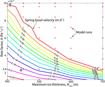
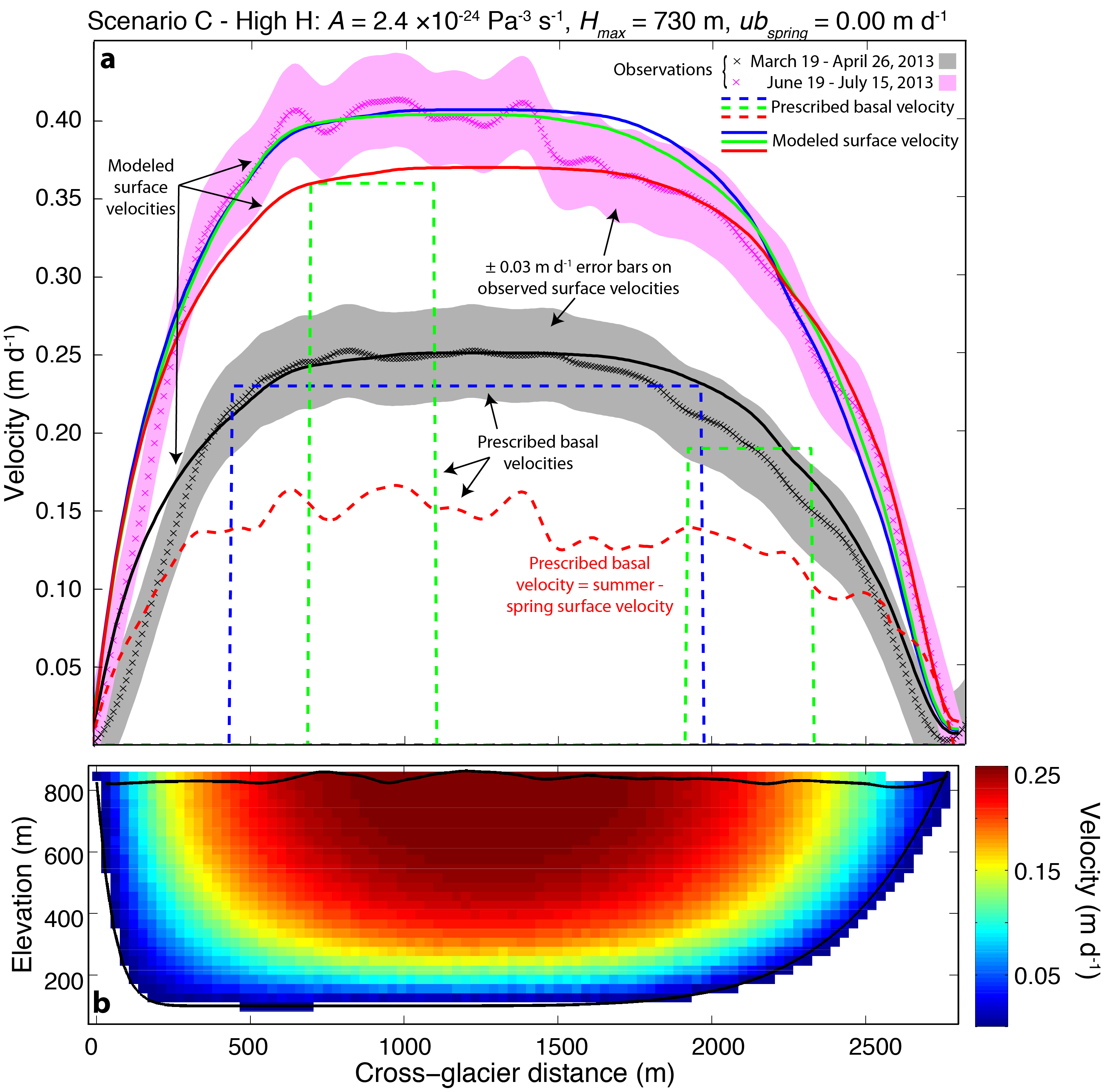
We consider three end-member scenarios, each of which reproduces the springtime surface velocities (Table 2; Figs 9, 10; Supplementary Fig. 2). In each of these scenarios, the influence of one of the factors (A, H max, springtime sliding) is emphasized. We do not claim that all these end-members are realistic, and present them only to demonstrate the sensitivity of inferred summer sliding to the assumed springtime conditions. All three scenarios considered reproduce the observed springtime surface velocities reasonably well, with RMSE values of 0.0155–0.0233 m d−1. The high-rate factor case (Scenario B; Fig. 10; Table 2) exhibited the lowest RMSE. The high spring basal speed case (Scenario A; Fig. 9; Table 2) had the highest RMSE. The high ice thickness case (Scenario C; Supplementary Fig. 2; Table 2) produced an intermediate RMSE but we do not include figures corresponding to this scenario in the main body of the paper in the interest of space. In Scenario A, in which we impose H max = 525 m and the standard A = 2.4 × 10⁻²⁴ Pa−3 s−1, a springtime basal velocity of 0.175 m d−1 (70% of the observed surface velocity) is required over 2/3 of the valley cross section to match the surface speed. This percentage of spring surface velocity attributable to basal motion is not outside the range of previously reported values of 50–90% (Raymond, Reference Raymond1971; Heinrichs and others, Reference Heinrichs, Mayo, Echelmeyer and Harrison1996; Truffer and others, Reference Truffer, Echelmeyer and Harrison2001; Amundson and others, Reference Amundson, Truffer and Luthi2006), although data on the average fraction of spring motion attributable to sliding is not readily available, especially for a non-surge type valley glacier. We first sought to restrict H max to 450 m for Scenario A to agree with radar estimates, but we were unable to explain the surface speedup without prescribing unrealistic basal velocity (e.g. basal velocity greater than the surface velocity or negative shear stresses); we have thus increased H max to 525 m for this scenario.
Results from Scenario A, which includes spring basal motion to match the observed spring surface speed. (a) Modeled ice surface speeds under several prescribed basal velocity scenarios. Crosses indicate observed velocities in spring (black) and mid-summer (pink); dashed lines indicate prescribed basal velocities in our 2-D cross-sectional flow model; solid lines show modeled ice surface velocities, where line colors indicate the corresponding basal velocity field. The basal velocity depicted by the red dashed line is equivalent to the measured summer speedup across the transect. The dotted lines show the summer increase in basal motion relative to spring. Model misfit and details are given in Table 2. (b) Modeled glacier geometry and associated model parameters (values in Table 2). Colors indicate out-of-plane (longitudinal) velocity.

Results from Scenario B, which employs a high rate factor (A) to match the observed spring surface speed. (a) Modeled ice surface speeds under several prescribed basal velocity scenarios. Crosses indicate observed velocities in spring (black) and mid-summer (pink); dashed lines indicate prescribed basal velocities in our 2-D cross-sectional flow model; solid lines show modeled ice surface velocities, where line colors indicate the corresponding basal velocity. The basal velocity depicted by the red dashed line is equivalent to the measured summer speedup across the transect. Model misfit and details are given in Table 2. (b) Modeled glacier geometry and associated model parameters (values in Table 2). Colors indicate out-of-plane (longitudinal) velocity.

Parameter choices for each end-member parameter sensitivity scenario and associated best-fitting basal slippery patch center location, width and magnitude of sliding velocity. ‘Base’ refers to parameters best fitting the spring velocity, ‘Uniform’ refers to a uniform sliding velocity within a single patch, and ‘Two patch’ refers to two slippery patches. ‘Speedup’ refers to prescribing the observed summer speedup as the basal velocity. For (A) the basal motion described in ‘uniform’ and ‘two patch’ is superimposed on top of ‘base’. The RMSE between modeled and measured surface velocities is shown in the last column

* Center location of the second slippery patch.
† Width of the second slippery patch.
Next, we seek to explain the observed summer velocities along the same transect by beginning from the three scenarios described above. We consider three schemes for specifying the basal velocity: a uniform sliding velocity along a fraction of the bed, high basal velocities in two ‘slippery’ patches, and a basal velocity equal to the summer speedup (i.e. taken as the difference between the observed summer and springtime surface velocities). In the first two schemes, we estimated the spatial distribution and magnitude of the additional basal velocity (i.e. over and above the springtime sliding velocity in Scenario A) required to match the observed summer velocities.
In the uniform sliding (i.e. single wide sliding patch) cases, additional basal velocities of 0.15–0.23 m d−1 over 64–54% of the bed, respectively, are required to match surface velocities (Table 2; Figs 9, 10). The width and magnitude of basal slip in the uniform sliding case is relatively insensitive to the choice of scenario. Note that in Scenario A, which includes spring sliding, the total basal velocity is 0.33 m d−1, the sum of the ‘base’ and ‘uniform’ cases in Table 2. While all of these three schemes produce a reasonable match to the maximum summer speeds, Scenarios A and C produce a superior fit (RMSE = 0.0260 and 0.0215, respectively; Table 2). Prescribing two narrower regions of high slip, basal velocities of 0.13–0.37 m d−1 over 43–22% of the bed, respectively, are required to match surface velocities (Table 2; Figs 9, 10). The model fits the observations slightly better for all scenarios in the two slippery patch case. In this case the width and magnitude of basal slip are sensitive to choice of scenario. The scenario with spring sliding (Scenario A) requires that a larger portion of the bed experience sliding than in Scenarios B and C to adequately explain the surface velocities. Prescribing the basal velocity as the surface speedup (i.e. difference between summer and spring surface velocities) under-predicts the peak surface velocity in all cases (Figs 9, 10) and generally yields intermediate-to-high RMSE when compared with the other basal slip cases (Table 2). That the basal velocity does not equal the summer speedup reflects cross-glacier stress gradient coupling that reduces the magnitude and widens the surface expression of basal motion (Section 5.2).
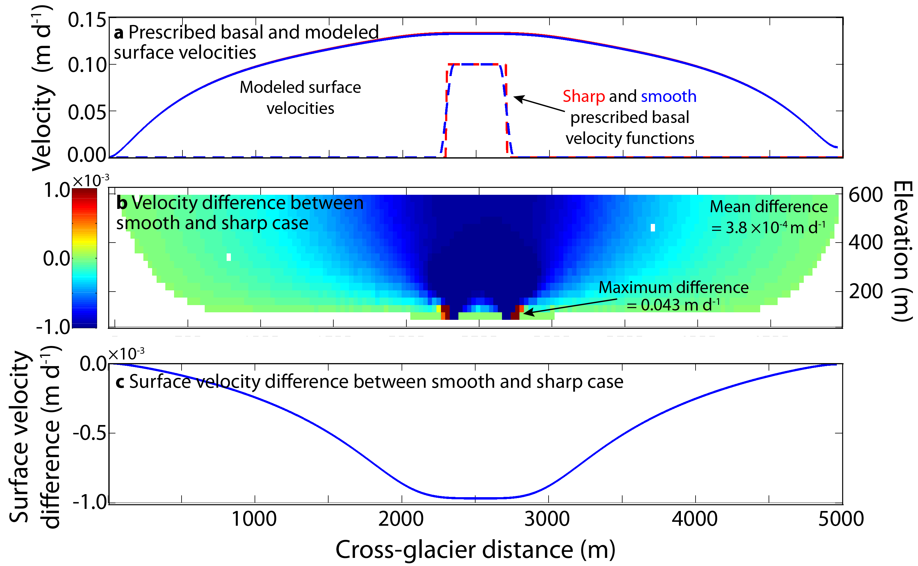
We are aware that the abrupt transition from zero to high basal velocity, as prescribed above, is unrealistic and can induce a non-physical basal traction field (Hutter and Olunloyo, Reference Hutter and Olunloyo1981; Schoof, Reference Schoof2004; Bueler and Brown, Reference Bueler and Brown2009). We analyze the shear stress field for each slip distribution case of each scenario and find the maximum basal shear stresses are generally within a plausible range of 100–150 kPa. We do have cases in which a negative basal shear stress is calculated at the transition between slip and no-slip boundary conditions, but this is generally limited to a small number of elements near the transition. The high spring sliding scenario (Scenario A) with two slippery patches, in which we impose the largest cross-glacier basal velocity gradients, produces the largest region of negative shear stresses. Previous authors have reported that this issue arises from a mathematical singularity at the transition from slip to no-slip (Hutter and Olunloyo, Reference Hutter and Olunloyo1981; Schoof, Reference Schoof2004; Amundson and others, Reference Amundson, Truffer and Luthi2006). We evaluate the model sensitivity to employing abrupt transitions in basal boundary condition by prescribing a smoothly varying basal velocity. We find the magnitude of the minimum basal shear stress increases (i.e. became less negative, or even positive), but observe no appreciable change in the overall pattern of ice deformation and surface velocity (Supplementary Fig. 3). For this reason, we use the simplest possible basal velocity patterns and do not parameterize the basal velocity with a continuous function.
5. DISCUSSION
5.1. Advantages of optical satellite image correlation
Our weekly-to-monthly averaged WorldView-derived glacier velocities (Fig. 4) agree remarkably well (to within 1% in both displacement magnitude and direction) with high-rate on-glacier differential GPS (Fig. 3). This approach provides much greater spatial coverage and resolution than GPS (5.6 m pixels over the terminal ~46 km2, compared with 1 GPS monument every ~3 km along a 15 km centerline transect), but sacrifices temporal resolution. The WorldView satellite repeat time is 16 d, which places a limit on the best possible temporal resolution of the method. Our method's coarse temporal resolution is counterbalanced by high spatial resolution and extent. Without large spatial coverage, for example, we would not be able to document the widespread uniformity of the summer speedup.
Unlike microwave-wavelength interferometric synthetic aperture radar (InSAR), extensive cloud cover precludes correlation of optical satellite imagery to produce velocity maps. As this is common in polar and alpine environments, velocity fields must often be averaged over longer timespans than the best-case 16 d window. Optical image correlation, however, appears to be more robust against temporal decorrelation, which is a difficulty for summertime InSAR velocity estimates (Burgess and others, Reference Burgess, Forster and Larsen2013). In addition, velocity estimation from InSAR is difficult on high-relief and time-variable surface elevations typical of alpine glaciers (Tedesco, Reference Tedesco2015). Our method of orthorectifying optical imagery with respect to the DEM produced from the concurrent stereopair reduces errors associated with changing glacier geometry, allowing for high-accuracy velocity determination on alpine glaciers.
5.2. Interpreting the spatiotemporal pattern of the summer speedup
The temporal evolution of glacier velocity (Figs 4, 5) is consistent with the cycle commonly observed on both alpine glaciers (e.g. Hooke and others, Reference Hooke, Calla, Holmund, Nilsson and Stroeven1989; Mair and others, Reference Mair, Nienow, Willis and Sharp2001; MacGregor and others, Reference MacGregor, Riihimaki and Anderson2005; Bartholomaus and others, Reference Bartholomaus, Anderson and Anderson2011) and Greenland outlet glaciers (Joughin and others, Reference Joughin2008; Sole and others, Reference Sole2011; Moon and others, Reference Moon2014) in which seasonal variability in both meltwater production and the evolving hydraulic system of the glacier result in fluctuations in subglacial water pressure and basal velocity (Iken and Bindschadler, Reference Iken and Bindschadler1986). We find that the speedup (summer minus spring surface velocity) reaches a maximum of ~0.15 m d−1 during early summer (19 June–15 July) and then declines through the end of our observation period (Fig. 6). The spatial distribution of the speedup is remarkably uniform, with a 12 km2 area speeding up by 0.15–0.20 m d−1 during the early summer (19 June–15 July; Figs 6a, 7a). The total ice surface velocity, in both spring and summer, varies significantly over this area (Figs 4, 7). At a given point, the early summer velocity is 1.4 to >10 times higher than the spring velocity, with areas of high spring speeds exhibiting smaller fractional velocity increases. The tenfold speedup is found near the lateral glacier margins and terminus, likely reflecting the influence of stress gradient coupling, as we discuss in greater detail below. The 40% relative speedup (1.4-fold velocity increase) found in faster-moving ice is similar to that observed on Greenland outlet glaciers (Hoffman and others, Reference Hoffman, Catania, Neumann, Andrews and Rumrill2011; Tedstone and others, Reference Tedstone, Nienow, Gourmelen and Sole2014).
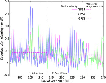
We consult our on-glacier GPS for the 15 July–1 August and 1–27 August image correlation timespans to ensure that this apparent spatial uniformity does not result from temporally averaging over spatially variable dynamics (e.g. wave-like propagation of regions of high basal motion; e.g. Kamb and Engelhardt, Reference Kamb and Engelhardt1987; Anderson and others, Reference Anderson2004; Harper and others, Reference Harper, Humphrey, Pfeffer and Lazar2007). We see no evidence for wave-like behavior; GPS velocities fluctuate on diurnal and multi-day timescales, but all stations vary synchronously (Fig. 11). We could not perform this analysis for the 19 March–26 April timespan because we only had 1 active GPS monument at that time; the same is true for the 15 June–19 July timespan due to GPS power loss.
Down-glacier velocity at three on-glacier GPS monuments, offset by subtracting the pre-spring event velocity at each station. Dashed lines show mean velocity over two WorldView image correlations. The mean speedup is uniform over this reach, while the spring velocities are 0.17 m d−1 at GPS3, 0.26 m d−1 at GPS4, and 0.31 m d−1 at GPS5. GPS3 is furthest down-glacier, with GPS4 and GPS5 located at ~3 and 6 km up-glacier, respectively.
As it is well recognized that the relationship between basal motion and its signature on the ice surface is complex (Balise and Raymond, Reference Balise and Raymond1985; Kamb and Echelmeyer, Reference Kamb and Echelmeyer1986; Gudmundsson, Reference Gudmundsson2003), we resort to modeling to explore how the signal of basal motion will be transmitted through the body of the glacier. As noted in Section 4.4, there are significant uncertainties involved in inferring basal motion based on the presently available data on Kennicott Glacier. Uncertainty in ice thickness particularly confounds efforts to infer basal motion. Even if the valley geometry were well constrained, our modeling results suggest that there is a tradeoff between the magnitude of the prescribed basal velocity and the proportion of the bed that is slipping, such that two end-member basal slip patterns (one in which a large portion of the bed slips at a moderate speed, the other in which a small portion of the bed slides rapidly) can produce similar surface velocities (Figs 9a, 10a). A relatively small basal velocity is required if much of the bed slips; this might simulate an extensive zone of high water pressure associated with a distributed drainage system (blue lines in Figs 9a, 10a). A wide, relatively uniform cross-sectional distribution of basal slip has been observed or inferred in several studies (Raymond, Reference Raymond1971; Truffer and others, Reference Truffer, Echelmeyer and Harrison2001; Amundson and others, Reference Amundson, Truffer and Luthi2006). If, on the other hand, a channelized drainage system is in place and a much smaller portion of the bed slips (perhaps due to high water pressure when the capacity of the channel is overwhelmed, for example, as observed and modeled by Hubbard and others, Reference Hubbard, Sharp, Willis, Nielsen and Smart1995; Werder and others, Reference Werder, Hewitt, Schoof and Flowers2013) then a much higher basal velocity is required to match the observed surface speedup (green lines in Figs 9a, 10a). It is interesting to note that the location of maximum summer speedup is offset from the glacier centerline (Figs 4, 6b) and, regardless of the chosen pattern for basal slip, our modeling suggests a higher basal velocity on the side of the bed into which the ice-marginal Hidden Creek Lake (HCL) would drain during its annual outburst flood (Figs 9a, 10a). The drainage of HCL produces an annual speedup event (Anderson and others, Reference Anderson, Walder, Anderson, Trabant and Fountain2005; Bartholomaus and others, Reference Bartholomaus, Anderson and Anderson2008), that occurred around 29 June in 2013 and is thus captured by the 19 June–15 July image correlation (Figs 4b, 6a). The higher basal sliding velocity in the left patch in Figures 9a, 10a could reflect HCL drainage altering basal conditions that in turn influence the speedup. Amundson and others (Reference Amundson, Truffer and Luthi2006) also inferred a region of high basal slip offset to one side on Black Rapids Glacier, which corresponds to the drainage pathway of an ice marginal lake.
The red lines in Figures 9a, 10a show the modeled surface velocity using the observed summer speedup as the input basal velocity distribution. Glaciological studies often interpret the difference between summer velocity and a minimum velocity observed in winter or spring as the ‘sliding speed’ at a point (e.g. Zwally and others, Reference Zwally2002; Anderson and others, Reference Anderson2004; Bartholomaus and others, Reference Bartholomaus, Anderson and Anderson2011; Tedstone and others, Reference Tedstone, Nienow, Gourmelen and Sole2014). We show here that while using the surface speedup as a proxy for the basal velocity may indeed account for the speedup field, there are many other plausible basal velocity patterns that can generate the same speedup pattern (Figs 9a, 10a). Previous studies have highlighted this point, demonstrating that neither the glacier surface velocity nor the basal velocity field are defined by local quantities (Kamb and Echelmeyer, Reference Kamb and Echelmeyer1986; Blatter and others, Reference Blatter, Clarke and Colinge1998; Price and others, Reference Price, Payne, Catania and Neumann2008). Prescribing the basal velocity based on the summer speedup leads to a slightly higher RMSE in fitting the surface velocity, compared with the two other prescribed sliding patterns. Stress gradient coupling reduces the magnitude and both spreads and smooths the surface expression of the prescribed basal sliding velocity; this creates the difficulty in distinguishing between these slip patterns and confounds interpretation of the difference between summer velocity and a winter/spring velocity at a point as the ‘sliding speed’ at that location.
The insensitivity of our modeled speedup to the prescribed basal velocity pattern likely reflects strong cross-glacier stress gradient coupling in the ice. The ice thickness at the location of the modeled transect is ~450 m (M. Truffer, 2014, unpublished data, personal communication), meaning that our observed speedup is uniform over ~12 (4) ice thicknesses in the down-glacier (cross-glacier) direction. This would be reduced to 10 (3) ice thicknesses if the large ice thickness Scenario C (Table 2; Supplementary Fig. 2) is closer to reality. While 4 ice thicknesses is the theoretically expected stress gradient coupling length scale for an alpine glacier, larger coupling length scales are expected when basal motion comprises a large fraction of ice surface displacement, potentially reaching 12 ice thicknesses for surging glaciers (Kamb and Echelmeyer, Reference Kamb and Echelmeyer1986). While Kennicott Glacier is not surging, its surface velocity may reflect a strong influence of basal motion (Fig. 9; Sections 4.4 and 5.2). If this is true, stress gradient coupling may largely explain the uniformity of the speedup. If background basal motion is less important (Fig. 10) and the coupling length scale is smaller, this leaves us with the alternative that there may exist a relatively uniform distribution of effective pressure at the bed driving uniform basal motion across this broad terminal region.
5.3. The difficulty in inferring basal conditions from the pattern of surface speedup
Motivated by the results presented in Section 4.4, we ask the question: when would we expect to be able to distinguish between several narrow slippery patches and one wide region of slip? The answer to this question is important for remotely sensed as well as field-based studies in which the goal is to infer basal slip and associated subglacial hydraulics from surface observations. We address this question using a numerical experiment in which we progressively widen the distance between two identical basal slippery spots and identify the separation distance required to resolve the two distinct slippery spots (Fig. 12).
Location of prescribed basal slip (dashed) and modeled surface velocities (solid) in a glacier with an aspect ratio of W/H = 40 (effectively infinitely wide). Surface velocity in the absence of basal motion is shown in black. Basal slip magnitude (u b/u def = 0.5) and extent (two patches λ = H/2 wide) is constant in all trials. We are unable to resolve individual slippery spots until they are separated by ≥4H.

We conducted these numerical experiments by non-dimensionalizing the problem, which collapses results from trials with disparate ice thicknesses, rate factors, aspect ratios and prescribed basal velocities. The results can be readily converted into dimensional units to consider a particular system of interest. We non-dimensionalize all lengths by the mean ice thickness (H),
 $${{y}_{{^\ast}}} = \displaystyle{{y} \over {H}};\quad {{\lambda} _{{^\ast}}} = \displaystyle{{\lambda} \over {H}};\quad and\quad {{W}_{{^\ast}}} = \displaystyle{{W} \over {H}}$$
where y is the cross-glacier coordinate, λ is the slippery patch width, and W is the glacier width. We non-dimensionalize surface and basal velocities by the expected deformation velocity calculated using the 1-D shallow ice approximation without a shape factor (i.e. infinitely wide glacier),
 $${{u}_{{^\ast}}} = \displaystyle{{{{u}_{s \vert b}}} \over {{{u}_{{\rm def}}}}} = \displaystyle{{{{u}_{s \vert b}}} \over {{\rm [2}{A}{\rm /}{n}{\rm + 1(}{\rho g}{\rm sin}{\alpha} {{\rm )}^{n}}\;{{H}^{{n}{\rm + 1}}}{\rm ]}}}$$
where u s|b is the surface or basal velocity, respectively, u def is the expected deformation velocity and the rest of the terms are defined in Section 3.4. We model the glacier using a nearly rectangular valley with wall steepness exponents of β = γ = 10 (Eqn (6)), a surface slope of 0.03 m m−1, and a rate factor of A = 2.4 × 10⁻²⁴ Pa−3 s−1 (Cuffey and Paterson, Reference Cuffey and Paterson2010).
In all trials, we assign λ = H/2, W = 40H and u b = u def/2. Between trials, we increase the separation distance between slippery patches from 0H to 16H and numerically model the surface velocity (Fig. 12). First, we note that at any separation distance, the surface expression of basal slip is distributed over a much wider distance than the region of active basal slip due to stress gradient coupling. At small separation distances, the basal drag associated with the intervening sticky spot is negligible and increasing the separation distance increases the maximum surface speedup. We find the maximum surface velocity occurs when the separation distance is equal to H/2 but note that the surface speedup is only 35% of the prescribed basal velocity (the ratio of modeled surface speedup to prescribed basal velocity increases to 1 as λ approaches W). As the separation distance is increased further, the maximum speedup decreases but a greater fraction of the surface experiences elevated velocity. Only when the separation distance is greater than 4H do the individual slippery spots express themselves in a ‘double humped’ speedup profile (Fig. 12). At this point, although the two slippery spots are resolvable in our model output, they would be extremely difficult to detect in noisy field observations of temporally varying surface velocities, until the separation distance is yet larger. Even when the separation distance is 20H the velocity difference between peak and trough is only ~0.1, which in dimensional terms would be 0.05 m d−1 for a glacier with a deformation velocity of 0.5 m d−1. This difference would be difficult to detect without very precise velocity measurements.
Adding to this difficulty, wall drag further damps any heterogeneity in the surface speedup in narrower glacier valleys (Fig. 13). In the ‘infinitely wide’ model (W/H = 40), the ‘double humped’ speedup pattern is just barely distinguishable at a separation distance of 4H. When W/H is decreased to 20, the two slippery spots are less recognizable in the surface velocity pattern and are indistinguishable when W/H = 10, most similar to that found in a confined valley glacier.
Comparison of the influence of prescribed basal velocities (dashed) on modeled surface speed (solid) on glaciers with varied aspect ratios. A double-humped speedup is evident in the W/H = 40 (infinitely wide case) and just barely in the W/H = 20 case. The surface expression of basal slip is muted in the W/H = 10 case (similar to Kennicott) due to wall friction and requirement of zero velocity at the glacier margins. Basal slip magnitude (u b/u def = 0.5) and extent (two patches λ = H/2 wide) is constant in all trials. The vertical offset between surface velocities is due to wall friction reducing the maximum surface velocity as W/H decreases.

In additional sensitivity studies, we found that the spatial distribution and magnitude of the surface speedup is sensitive to the width of the slipping region, as well as the magnitude of the prescribed basal velocity relative to the glacier's deformation velocity, but not to the rate factor A, per se. That is, in model runs with differing A, the surface speedup in response to a given basal velocity field will be exactly the same if the surface slope increases to compensate for a lower A such that the deformation velocity (term in brackets in Eqn (8)) is constant (Supplementary Fig. 4). By rearranging Eqns (3) and (4) such that both A and α appear in the driving stress term, it is readily seen that the velocity solution is unchanged for identical values of the product of A1/n and sin(α).
The above results indicate that we cannot expect to resolve variations in basal motion from surface observations until those variations occur over distances many times the ice thickness. These findings echo those of previous authors who found basal perturbations are not faithfully transmitted to the surface until those perturbations occur on a length scale equivalent to many times the ice thickness (Balise and Raymond, Reference Balise and Raymond1985; Kamb and Echelmeyer, Reference Kamb and Echelmeyer1986; Raymond and Gudmundsson, Reference Raymond and Gudmundsson2005). We therefore argue that the influence of cross-glacier stress gradient coupling between regions of low and high effective pressure (Blatter and others, Reference Blatter, Clarke and Colinge1998; Price and others, Reference Price, Payne, Catania and Neumann2008) can explain the widespread uniformity of surface speedups in valley glaciers (and ice sheets, although to a lesser extent due to their closer similarity to the infinitely wide case) as well as other alternative mechanisms that have been proposed, such as uniform hydrology (e.g. Tedstone and others, Reference Tedstone, Nienow, Gourmelen and Sole2014). This is true for any glacier but in situations where basal slip contributes significantly to surface velocity, the effective ice coupling length scale increases (Kamb and Echelmeyer, Reference Kamb and Echelmeyer1986; Gudmundsson, Reference Gudmundsson2003), and slippery spots must be even further separated before they are resolved in the ice surface speedup.
5.4. Implications for glacier models
A major confounding factor in unraveling the mechanisms controlling basal motion on Kennicott Glacier is the poorly constrained basal geometry. As a result, there is a tradeoff between ice thickness, flow law parameter A, and springtime background basal velocity; and springtime motion may be explained by several end-member scenarios (Figs 9, 10, Supplementary Fig. 2, Table 2). However, we also find that several end-member basal velocity configurations can explain the summer speedup equally well (Figs 9a, 10). One model run is meant to simulate widespread basal slip associated with a distributed cavity drainage system, while another simulates high localized slip that may occur near overwhelmed channelized drainage. Our third test case does nearly as well (although it generally produces the highest RMSE) by employing a common glaciological practice of estimating the basal velocity as the difference between summer and early spring surface velocity. While this non-uniqueness frustrates the exercise of probing basal phenomena using surface data, it offers promise for numerical modeling efforts of glaciers and ice sheets. If disparate basal slip patterns can explain our observed summer speedup equally well, then it is less important to know the detailed slip pattern to accurately predict integrated glacier behavior. Indeed, Tedstone and others (Reference Tedstone, Nienow, Gourmelen and Sole2014) found that proximity to an inferred subglacial conduit is unimportant for determining the proportion of annual motion that is accomplished in summer, and suggest that a high-complexity description of subglacial hydraulics may not be required for accurate ice flow models. Our findings echo these results. Presumably basal hydraulic conditions vary considerably over our study reach in both space and time, and yet we find a uniform speedup magnitude over a length scale equal to 12 (4) ice thicknesses in the down- (cross) glacier direction. Our modeling results show that strong cross-glacier stress gradient coupling effectively acts to smooth variations in basal velocity, resulting in similar surface speedup patterns despite varied basal velocity configurations (Figs 9, 10, 12, 13). This may allow for simpler parameterizations of the increased ice flux associated with hydraulically-induced speedup without requiring a detailed description of basal conditions.
6. CONCLUSIONS
We document the evolution of ice surface velocity on Kennicott Glacier from 19 March–27 August 2013 using cross correlation of WorldView optical satellite imagery. We find the satellite-derived velocity estimates agree with on-glacier GPS motion to within 1% in both displacement azimuth and magnitude. The high-spatial resolution of WorldView imagery allows analysis of glacier dynamics over intra-seasonal timescales. We document the often-observed cycle in which glacier velocity reaches a maximum in early summer and slows until fall. The summer speedup is much more uniform than the spring ice surface speed, indicating that the pattern of the summer speedup cannot simply be assumed to be a scaled version of the deformation velocity field, at least in the terminal reach of this alpine glacier. We employ a 2-D cross-sectional numerical flow model in an attempt to explain the observed spring surface velocity field but are unable to distinguish between widely distributed moderate-speed basal motion and narrower high basal velocity zones from surface observations. Our modeling shows that ice surface velocities cannot reveal distinct regions of high basal velocity until they are separated by at least four ice thicknesses, and that this problem is exacerbated by the relatively low width-to-depth ratios of alpine glaciers such as Kennicott. The insensitivity of the glacier surface velocity to the details of the basal velocity field reflects the influence of strong transverse and longitudinal stress gradient ice coupling in determining the ice surface velocity, but may provide an excuse to employ simpler representations of glacier basal hydraulics in glacier models.
SUPPLEMENTARY MATERIAL
The supplementary material for this article can be found at http://dx.doi.org/10.1017/jog.2016.66.
ACKNOWLEDGEMENTS
We thank Assistant Editor Helen Fricker, Martin Truffer and an anonymous reviewer for detailed and thoughtful comments that greatly improved the quality of this manuscript. We thank Sebastien Leprince for patient help in employing COSI-Corr. In addition, we thank Spencer Niebuhr, Claire Porter, George Roth, Paul Morin and the Polar Geospatial Center for providing WorldView imagery. We are grateful to the following people and organizations for assistance with fieldwork: Katy Barnhart, Andy Wickert, Connor Simmons, Hannah Grist, Emily Baker, Pablo y Olga, Blair Hensen, Will van Gelder, Dasan Mitchell, Aleah Sommers, Mike Loso, Tim Bartholomaus, Michael Spehlmann, Seth Stockton, the Wrangell Mountains Center, Wild Alpine Guides, St. Elias Alpine Guides, Keith and Laurie Rowland, Paul Claus, Peter and Katie Hauessler, and Tess Cecil-Cockwell and Zach McMahon. WHA, RSA, and HR acknowledge funding from the National Science Foundation grant EAR-1548725. JA and HR acknowledge funding from NASA project ROSES NNX12AB72G.


 Open access