2. RELATED WORKS

SLAM is a technique that allows the creation of a map of a previously unknown environment, which is then used for navigation during further operations in the area. This positioning method was first recognised in 1986 (Durrant-Whyte and Bailey, Reference Durrant-Whyte and Bailey2006). During this time, preliminary attempts were made to implement the elements of probability theory for robot navigation. It was at that time that it was established that mapping the space around the object and then using it for auto-location was a fundamental problem that would have to be tackled in the future (Cadena et al., Reference Cadena, Carlone, Carrillo, Latif, Scaramuzza, Neira, Reid and Leonard2016). The vast majority of the work on the subject related to SLAM is based on the Extended Kalman Filter (EKF) (López et al., Reference López, García, Barea, Bergasa, Molinos, Arroyo and Pardo2017; Thrun et al., Reference Thrun, Burgard and Fox2005; Gérossier et al., Reference Gérossier, Checchin, Blanc, Chapuis and Trassoudaine2009) or its modifications (Yuan et al., Reference Yuan, Martínez-Ortega, Fernández and Eckert2017; Reference Yuan, Martínez, Eckert and López-Santidrián2016). For the purpose of this positioning technique, a range of environment mapping sensors can be used, ranging from cameras through ultrasonic distance sensors to laser scanners. Currently, there is a strong emphasis on the processing of image data from single or circular cameras (Li, Reference Li2008; Lu, Reference Lu2016) in order to obtain an image of the environment, which is the point cloud. This trend continues due to availability of Intel's Open source Computer Vision (OpenCV) and Mobile Robot Programming Toolkit (MRPT) image processing libraries, which are open source libraries enabling the fusion of data from a variety of sensors. The optimisation of development tools in terms of performance enabled the processing of graphic elements in almost real time, which solves the problem of online work. The visualisation of the measured model of the environment is then used to build a Three-Dimensional (3D) map of the robot's operating environment. This use of the 3D model enables the distinguishing of many more special points and environmental features as compared to 2D mapping. These points – landmarks – are later used in finding the location of the vehicle using EKF methods (Aguilar-Gonzáles, Reference Aguilar-Gonzáles2016; Paz, Reference Paz2008; Castellanos et al., Reference Castellanos, Martínez, Neira and Tardós1998), Unscented Kalman Filter (UKF) (Montemerlo et al., Reference Montemerlo, Thrun, Koller and Wegbreit2002) and MonteCarlo (Dissanayake, Reference Dissanayake2001).

Since the beginning of this decade, the emphasis has been put on the use of the only sensor in SLAM that maps the surroundings available on the majority of seagoing vessels, namely the navigational radar (Rouveure et al., Reference Rouveure, Faure and Monod2010). Previous work on the use of SLAM technology based on radar indicates a drift of both the vessel's position and the estimates of its course and speed over time, as it moves away from the location where positioning started. This is the result of the characteristics of the EKF. The phenomenon of drift of position coordinates is related to the characteristics of an error in dead reckoning, the precision of which decreases in time. The EKF tries to establish a trade-off between the estimated observed position and the coordinates resulting from mathematical calculations in dead reckoning. How the elements related to the cumulative mathematical error will affect the positioning errors should be considered. Another problem worth considering is the appropriate configuration of the navigational infrastructure. It is assumed that the appropriate location of the navigational marking would allow for positioning based on the EKF SLAM method in accordance with the IMO accuracy criteria for navigation in port approach waters.

3. THE MATHEMATICAL MODEL

While determining a location based on the SLAM EKF method, a robot tries to determine its location and orientation $\boldsymbol{\xi}_{k}$ as well as a discrete map of the surrounding landmarks (in this paper, beacons) $\textbf{M}_{k}$ at the current moment k. This is usually done on a regular basis, in a previously set up discrete moment k≥0. This paper assumes that the environment in which the vessel's motion has been simulated is a two-dimensional plane in the local reference system, and therefore $\boldsymbol{\xi}_{k} \triangleq (x_{k}\ y_{k}\ \theta_{k})^{{\rm T}}$, where the vessel's position $(xs_{k}\ ys_{k})\in {\mathbb R}^{2}$ and the vessel's COG value is $\theta_{k} \in \langle 0, 2\Pi\rangle$. The map of the environment in the computer simulation $\textbf{M}_{k} =(x_{1}\ y_{1}\cdots x_{i}\ y_{i})^{{\rm T}}$ will be represented as a vector storing the positions of the navigational aids (beacons), where their number will be $\mbox{i}\in {\mathbb Z}$ and $\mbox{i}\in \langle 1,2\rangle,4$ depending on the test variant.

It has been assumed that the starting position xs _k=0, ys _k=0, from which the vessel starts navigating has a zero mean directional error.

(1)$$\begin{align} &\sigma_{xs_0}=0\label{eq1} \end{align}$$

(2)$$\begin{align} &\sigma_{ys_0}=0\label{eq2} \end{align}$$

During the movement on the fairway, the vessel starts its journey at a constant speed over the ground V _k=const in time and at a constant rate of increase of change of course over ground ROT _k=const. The motion model of a vessel at a discrete time can be expressed in the following function (motion control $\textbf{u}_{k}$ is assumed to be known):

(3)$$\textbf{x}_k =g( {{\textbf{x}}_{k-1}, {\textbf{u}}_k })=\left[ {{\begin{matrix} {xs_k } \\ {ys_k } \\ {\theta_k } \\ \end{matrix} }} \right]=\left[ {{\begin{matrix} {xs_{k-1} +V_k \cdot (t_k -t_{k-1} )\cdot \cos( {\theta_{k-1} } )}\\ {ys_{k-1} +V_k \cdot(t_k -t_{k-1} )\cdot\sin( {\theta_{k-1} } )}\\ {\theta_{k-1} +ROT_k \cdot(t_k -t_{k-1} )} \end{matrix} }} \right]$$

The value of the increase in the course of the vessel over ground ROT _k and velocity V _k are affected by a random error with a normal distribution of σ_ROT, σ_V:

(4)$$\begin{align} \Delta V_k &\sim {\mathbb N}(0, \sigma_v^{2})\label{eq4} \end{align}$$

(5)$$\begin{align} \Delta ROT_k &\sim {\mathbb N}(0, \sigma_{ROT}^{2})\label{eq5} \end{align}$$

The EKF SLAM method requires the estimation of the position of the observed beacons. In order to determine the position of the jth beacon, a series of measurements must be taken to determine the distance z _r and bearing z _β to the aid. The measurement vector is indicated by ${\textbf{z}}=(z_{r},z_{\beta})^{{\rm T}}$. It was assumed that both the vessel and the navigational aids are objects with dimensions $1\,{\rm m}\times 1\,{\rm m}$. The centroid of the square representing the object was assumed to be the location of the beacon. The position of the object was fixed and did not move (float) during a pass of a simulated vessel. The measurements have a random error Δ z _r, $\Delta z_{\beta}$ of normal distribution with the standard deviation previously assumed and typical for the radar/LIDAR type device: σ_r for distance measurement, $\sigma_{\beta}$ for bearing measurement. The measurement model to i of this aid is expressed in the following function:

(6)$${h_i}({{\bar{\textrm x}}_k}) = \left[ {\begin{array}{*{20}{c}} {{z_r}}\\ {{z_\beta }} \end{array}} \right] = \left[ {\begin{array}{*{20}{c}} {\sqrt {{{\left( {{x_i} - x{s_k}} \right)}^2} + {{\left( {{y_i} - y{s_k}} \right)}^2}} }\\ {ta{n^{ - 1}}\left( {\frac{{{y_i} - y{s_k}}}{{{x_i} - x{s_k}}}} \right) - {\theta _k}} \end{array}} \right]$$

(7)$$ \Delta z_r \sim {\mathbb N}( {0,\sigma_r^2} ) $$

(8)$$\Delta z_{\beta} \sim {\mathbb N}( {0,\sigma_{\beta}^2} ) $$

4. EKF IN SLAM

As is generally known, the movement of a vessel is not linear. We can observe that in most cases a generalisation of the shape of the vessel's trajectory when Δ t→0 can be the section of a circle. That is why the Extended Kalman Filter has been used to estimate the position of the ship. It linearizes processes considered to be non-linear in the local area. The Taylor series of the first order is used for this purpose. The general algorithm of the Extended Kalman Filter is very similar to the basic Kalman Filter (KF) version and is as follows: Extended Kalman filter $({\textbf{x}}_{k-1},{\textbf{P}}_{k-1},{\textbf{u}}_{k},{\textbf{z}}_{k})$:

(9)$$\begin{align} \bar{\textbf{x}}_{k}&=g( {\textbf{x}}_{k-1},{\textbf{u}}_{k}) \label{eq9} \end{align}$$

(10)$$\begin{align} \bar{\textbf{P}}_{k}&=( {\textbf{G}}_{k}\cdot {\textbf{P}}_{k-1}\cdot\textbf{G}_{k}^{{\rm T}}+{\textbf{R}}_{k} ) \label{eq10} \end{align}$$

(11)$$\begin{align} {\textbf{K}}_{k}&=\bar{\textbf{P}}_{k}\cdot {\textbf{H}}_{k}^{{\rm T}}\cdot {({\textbf{H}}_{k}\cdot\bar{\textbf{P}}_{k}\cdot {\textbf{H}}_{k}^{{\rm T}}+{\textbf{Q}}_{k})}^{-1}\label{eq11} \end{align}$$

(12)$$\begin{align} {\textbf{x}}_{k}&=\bar{\textbf{x}}_{k}+{\textbf{K}}_{k}\cdot ({\textbf{z}}_{k}-h(\bar{\textbf{x}}_{k}))\label{eq12} \end{align}$$

(13)$$\begin{align} {\textbf{P}}_{k}&=({\textbf{I}}-{\textbf{K}}_{k}\cdot {\textbf{H}}_{k})\cdot\bar{\textbf{P}}_{k}\label{eq13} \cr \hbox{return} \textbf{x}}_{k}, \textbf{P}}_{k}\end{align}$$

where ${\textbf{x}}_{k}$ is the state vector storing the positions of the vessel and the navigational aids, ${\textbf{P}}_{k}$ is the covariance matrix of position errors of the vessel and navigational aids, ${\textbf{K}}_{k}$ is the EKF-specific weight matrix, ${\textbf{Q}}_{k}$ is the covariance matrix of the measurement model, ${\textbf{R}}_{k}$ is the covariance matrix of the motion model errors, ${\textbf{G}}_{k}$ is the Jacobian of the function g(·) with respect to system state and ${\textbf{I}}$ is the identity matrix.

5. ALGORITHM

In the simulation study, the algorithm of the SLAM Extended Kalman Filter was divided into three data processing phases. The first phase was the initialisation of the filter. In the simulation made for the purposes of the article, it takes place once at the beginning of the study and after changing the location of at least one navigational aid. The initial values are assigned to matrices, vectors and all variables in this step. The following are determined as assumed in the study: the speed over ground V ₀, the number of navigational aids (beacons) i, the initial course over ground θ₀, the number of calculation steps j sufficient to travel the distance constituting the entire waterway at a fixed speed xs ₀, the initial location of the vessel ys ₀ and the actual positions of the navigational aids $x_{0},y_{0},\ldots,x_{i},y_{i}$, which are required for estimating the coordinates of the position of the vessel. In addition, the initial values of the covariance matrix ${\textbf{P}}_{0}$ are determined:

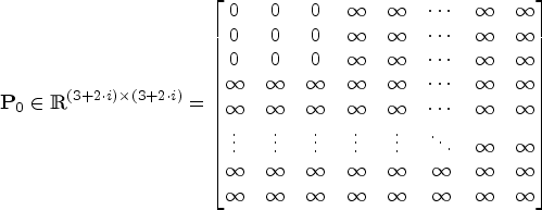(14)$${\textbf{P}}_0 \in {\mathbb R}^{(3+2\cdot i)\times (3+2\cdot i)}=\left[ {{\begin{matrix} 0 & 0 & 0 & \infty & \infty & \cdots& \infty & \infty \\ 0 & 0 & 0 & \infty & \infty & \cdots& \infty & \infty \\ 0 & 0 & 0 & \infty & \infty & \cdots& \infty & \infty \\ \infty & \infty & \infty & \infty & \infty& \cdots & \infty & \infty \\ \infty & \infty & \infty & \infty & \infty& \cdots & \infty & \infty \\ \vdots & \vdots & \vdots & \vdots & \vdots& \ddots & \infty & \infty \\ \infty & \infty & \infty & \infty & \infty& \infty & \infty & \infty \\ \infty & \infty & \infty & \infty & \infty& \infty & \infty & \infty \end{matrix} }} \right]$$

The covariance matrix ${\textbf{P}}_{k} $ is a block matrix. Elements of the matrix ${\textbf{P}}_{0} \in {\mathbb R}^{3\times 3}$ are related to mean errors of coordinates of the vessel's position and course, as well as with mutual covariations of coordinates of the position and course. During initialisation, the block is filled with zeroes, which is due to the lack of uncertainty regarding the initial values of the course and the location of the ship. The values of the remaining elements of the matrix are set at very high values, so that they go to infinity. This is due to the fact that the positions of the navigational aids are not known at the time of filter initialisation, so the error of their positions is infinitely great. In fact, the error value was assumed at 10⁶ m for the purpose of the simulation. After the initial values of the covariance matrix have been determined, the initial state vector ${\textbf{x}}_{0}$ is also initialised:

(15)$${\textbf{x}}_0 \in {\mathbb R}^{3+2\cdot i}=\left[ {{\begin{matrix} {xs_k } & {ys_k } & {\theta_0 } & 0 & \cdots & 0 \end{matrix} }} \right]^{{\rm T}}$$

The error values of average distance and bearing measurements and speed of the vessel are determined, as well as changes in the course in matrices ${\textbf{M}}$ and ${\textbf{Q}}$:

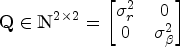(16)$$\begin{align} {\textbf{Q}}\in {\mathbb N}^{2\times 2}&=\left[ {{\begin{matrix} {\sigma_r^2} & 0 \\ 0 & {\sigma_\beta^2} \end{matrix} }} \right]\label{eq16} \end{align}$$

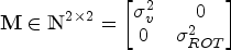(17)$$\begin{align} {\textbf{M}}\in {\mathbb N}^{2\times 2}&=\left[ {{\begin{matrix} {\sigma_v^2} & 0 \\ 0 & {\sigma_{ROT}^2} \\ \end{matrix} }} \right]\label{eq17} \end{align}$$

where σ_r is the mean error of distance measurement to the navigational aid, $\sigma_{\beta} $ is the mean error of the bearing measurement to the navigational aid, σ_v is the mean error of Speed Over Ground (SOG) measurement and σ_ROT is the mean error of the Rate Of Turn (ROT) measurement.

The next step is prediction. During this step, the position of the vessel ${\boldsymbol{\xi }}_{k} $ is estimated based on the readings of course over ground, speed above ground and its last position ${\boldsymbol{\xi }}_{k-1} $. The determination of the dead reckoning position and course is based on the Equation (9) state transition model equation of the system. This equation refers to the model of motion of the vessel contained in Equation (3). The prediction stage uses the function g(·) to incorporate the control ${\textbf{u}}_{k}$ into the estimated coordinates of the position $\bar{\textbf{x}}_{k}^{0{\cdot}3}$.

(18)$$\bar{\textbf{x}}_{k}^{0{\cdot}3}=\left[ {\begin{matrix} {xs}_{k}\\ {ys}_{k}\\ \theta_{k}\\ \end{matrix} } \right]=\left[ {\begin{matrix} {xs}_{k-1}\\ {ys}_{k-1}\\ \theta_{k-1}\\ \end{matrix} } \right]+\left[ {\begin{matrix} V_{k}\cdot (t_{k}-t_{k-1})\cdot\cos (\theta_{k-1})\\ V_{k}\cdot (t_{k}-t_{k-1})\cdot\sin (\theta_{k-1})\\ {ROT}_{k}\cdot(t_{k}-t_{k-1}) \end{matrix} } \right]$$

Next, the function's Jacobian is created g(·), with respect to the system state:

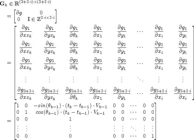(19)$$\begin{align} &{\textbf{G}}_k \in {\mathbb R}^{( {3+2\cdot i} ) \times ( {3+2\cdot i}) }\notag\\ &\quad =\left[\begin{matrix} {\partial g} & 0 \\ 0 & {{\textbf{I}}\in {\mathbb Z}^{2\cdot i\times 2\cdot i}} \\ \end{matrix}\right]\notag\\ &\quad =\left[\begin{matrix} \dfrac{\partial g_{1}}{\partial {xs}_{k}} & \dfrac{\partial g_{1}}{\partial {ys}_{k}} & \dfrac{\partial g_{1}}{\partial \theta_{k}} & \dfrac{\partial g_{1}}{\partial x_{1}} & \dfrac{\partial g_{1}}{\partial y_{1}} & \cdots & \dfrac{\partial g_{1}}{\partial x_{i}} & \dfrac{\partial g_{1}}{\partial y_{i}}\\ \noalign{\vskip6pt} \dfrac{\partial g_{2}}{\partial {xs}_{k}} & \dfrac{\partial g_{2}}{\partial {ys}_{k}} & \dfrac{\partial g_{2}}{\partial \theta_{k}} & \dfrac{\partial g_{2}}{\partial x_{1}} & \dfrac{\partial g_{2}}{\partial y_{1}} & \cdots & \dfrac{\partial g_{2}}{\partial x_{i}} & \dfrac{\partial g_{2}}{\partial y_{i}}\\ \noalign{\vskip6pt} \dfrac{\partial g_{3}}{\partial {xs}_{k}} & \dfrac{\partial g_{3}}{\partial {ys}_{k}} & \dfrac{\partial g_{3}}{\partial \theta_{k}} & \dfrac{\partial g_{3}}{\partial x_{1}} & \dfrac{\partial g_{3}}{\partial y_{1}} & \cdots & \dfrac{\partial g_{3}}{\partial x_{i}} & \dfrac{\partial g_{3}}{\partial y_{i}}\\ \noalign{\vskip6pt} \vdots & \vdots & \vdots & \vdots & \vdots & \ddots & \vdots & \vdots \\ \noalign{\vskip6pt} \dfrac{\partial g_{3+2\cdot i}}{\partial {xs}_{k}} & \dfrac{\partial g_{3+2\cdot i}}{\partial {ys}_{k}} & \dfrac{\partial g_{3+2\cdot i}}{\partial \theta_{k}} & \dfrac{\partial g_{3+2\cdot i}}{\partial x_{1}} & \dfrac{\partial g_{3+2\cdot i}}{\partial y_{1}} & \cdots & \dfrac{\partial g_{3+2\cdot i}}{\partial x_{i}} & \dfrac{\partial g_{3+2\cdot i}}{\partial x_{i}} \end{matrix}\right]\notag\\ &\quad =\left[ {\begin{matrix} 1 & 0 & -sin(\theta_{k-1})\cdot (t_{k}-t_{k-1})\cdot V_{k-1} & 0 & 0 & \cdots & 0 & 0\\ 0 & 1 & cos(\theta_{k-1})\cdot (t_{k}-t_{k-1})\cdot V_{k-1} & 0 & 0 & \cdots & 0 & 0\\ 0 & 0 & 1 & 0 & 0 & \cdots & 0 & 0\\ \vdots & \vdots & \vdots & \vdots & \vdots & \ddots & \vdots & \vdots \\ 0 & 0 & 0 & 0 & 0 & \cdots & 0 & 1 \end{matrix} } \right]\label{eq19} \end{align}$$

Once the required matrix has been determined, the current values of the covariance matrix ${\textbf{P}}_{k} $ are calculated. The first part of the ${\textbf{G}}_{k} {\textbf{P}}_{k-1} {\textbf{G}}_{k}^{\textbf{T}} $ equation is intended to propagate the uncertainty of the estimate of the items from the state k−1 to the state k. On the other hand, the matrix ${\textbf{R}}$ causes the inclusion of additional uncertainty caused by noisy, error-prone indications of the value of the assumed motion control ${\textbf{u}}_{k} $ into the filter system and is defined as:

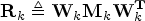(20)$$\begin{align} {\textbf{R}}_k &\triangleq {\textbf{W}}_k {\textbf{M}}_k{\textbf{W}}_k^{\textbf{T}}\label{eq20} \end{align}$$

(21)$$\begin{align} {\textbf{R}}_k &\in {\mathbb N}^{( {3+2\cdot i} ) \times ( {3+2\cdot i}) }.\label{eq21} \end{align}$$

Designation of the matrix ${\textbf{R}}_{k} $ requires the calculation of Jacobian $g( \cdot) $, with respect to noisy control input:

(22)$${\textbf{W}}_{k}\in {\mathbb R}^{(3+2\cdot i)\times 2}=\left[ \begin{matrix} \dfrac{\partial g_{1}}{\partial V_{k}} & \dfrac{\partial g_{1}}{\partial \theta_{k}}\\ \noalign{\vskip6pt} \dfrac{\partial g_{2}}{\partial V_{k}} & \dfrac{\partial g_{2}}{\partial\theta_{k}}\\ \noalign{\vskip6pt} \dfrac{\partial g_{3}}{\partial V_{k}} & \dfrac{\partial g_{3}}{\partial\theta_{k}}\\ \noalign{\vskip6pt} \vdots & \vdots \\ \noalign{\vskip6pt} \dfrac{\partial g_{3+2\cdot i}}{\partial V_{k}} & \dfrac{\partial g_{3+2\cdot i}}{\partial \theta_{k}} \end{matrix}\right]$$

The entire equation on the covariance matrix ${\textbf{P}}_{k} $ is represented as follows:

(23)$$\bar{\textbf{P}}_{k}={\textbf{G}}_{k}{\textbf{P}}_{k-1}{\textbf{G}}_{k}^{{\textbf{T}}}+{\textbf{W}}_{k}{\textbf{M}}_{k}{\textbf{W}}_{k}^{{\rm T}}$$

The next step of the EKF operation is the correction phase. The filtration algorithm incorporates a set of randomly errored measurements ${\textbf{z}}_{k} $ into the observed navigational aids Equation (12). The prediction step starts the determination of the weight matrix. Based on the current covariance matrix determined at an earlier stage, it indicates how much the results of measurement ${\textbf{z}}_{k} $ will affect ${\boldsymbol{\xi }}_{k}$. The weight matrix ${\textbf{K}}_{k} $ is defined as:

(24)$${\textbf{K}}_{k}\in {\mathbb R}^{(3+2\cdot i)\times 2}={\textbf{K}}_{k}=\bar{\textbf{P}}_{k}\cdot {\textbf{H}}_{k}^{\mathrm{T}}\cdot {({\textbf{H}}_{k}\cdot \bar{\textbf{P}}_{k}\cdot {\textbf{H}}_{k}^{\mathrm{T}}+{\textbf{Q}}_{k})}^{-1}$$

where ${\textbf{H}}_{k} $ is a Jacobian of the measurement model function $h( \cdot) $ with respect to system state:

(25)$${\textbf{H}}_{k}\in {\mathbb R}^{2\times ( 3+2\cdot i ) }=\left[ {\begin{matrix} \dfrac{\partial h_{1}}{\partial {xs}_{k}} & \dfrac{\partial h_{1}}{\partial {ys}_{k}} & \dfrac{\partial h_{1}}{\partial \theta_{k}} & \dfrac{\partial h_{1}}{\partial x_{1}} & \dfrac{\partial h_{1}}{\partial y_{1}} & \cdots & \dfrac{\partial h_{1}}{\partial x_{i}} & \dfrac{\partial h_{1}}{\partial y}\\ \noalign{\vskip6pt} \dfrac{\partial h_{2}}{\partial {xs}_{k}} & \dfrac{\partial h_{2}}{\partial {ys}_{k}} & \dfrac{\partial h_{2}}{\partial \theta_{k}} & \dfrac{\partial h_{2}}{\partial x_{1}} & \dfrac{\partial h_{2}}{\partial y_{1}} & \cdots & \dfrac{\partial h_{2}}{\partial x_{i}} & \dfrac{\partial h_{2}}{\partial y_{i}} \end{matrix}}\right]$$

The corrected covariance matrix is generated as follows:

(26)$${\textbf{P}}_{k}\in {\mathbb R}^{(3+2\cdot i)\times (3+2\cdot i)} =({\textbf{I}}-{\textbf{K}}_{k}\cdot {\textbf{H}}_{\mathbf{k}})\cdot \bar{\textbf{P}}_{k}$$

and the state vector ${\textbf{x}}_{k} $ is corrected based on the series of measurements for the navigation (beacons) aids according to the formula:

(27)$${\textbf{x}}_{k}=\bar{\textbf{x}}_{k}+{\textbf{K}}_{k}\cdot ({\textbf{z}}_{k}-h(\bar{\textbf{x}}_{k}))$$

The last two steps of filtration, that is, prediction and correction phases, take place in a loop. The number of repetitions j depends on the value of time assumed in the study, which will allow the vessel to cover the assumed distance. This route is the same throughout the simulation study, which affects the unchanging value of the variable j.

6. EXHAUSTIVE SEARCH METHOD

For many problems, finding the algorithm which directly constructs a solution is impossible or too difficult. In this case, an exhaustive search method may be used to analyse all potential solutions and select those that fulfil the conditions of the task. An exhaustive search can be time-consuming, as the number of potential solutions often increases exponentially with the size of the input data (Czech et al., Reference Czech, Deorowicz and Fabian2010).

The exhaustive search method is an iterative way to find a correct solution to a research problem by considering all possible combinations of data (Figure 1). For the described research problem, the time-consuming nature of the solution can be negligible to some extent, because the test takes place only once. However, assuming too many combinations of locations for navigational aids can result in a very long calculation time even on a computer with a high processing power. In order to reduce the number of combinations, zones were delimited in which the navigational aids do not appear. For the positioning of the navigational aids at every possible point of the considered area, chosen by the author of the study, it was assumed:

Figure 1.

Graphical representation of the method of changing the position of navigational aids for (a) i=2 and (b) i=4.

In order to reduce the number of cases, it was found that the following resolution values should be adopted between the two locations of the navigational aid during the simulation study:

$$ \hbox{for }i=1{:}\ res=10\,\mbox{m};\hbox{ for }i=2{:}\ res=50\,\mbox{m};\hbox{ for }i=4{:}\ res=100\,\mbox{m}. $$

7. SIMULATION STUDY

It was assumed that the examined area would be the approach to the Main Entrance of the Port of Gdynia located in Gdańsk Bay. The water area is oriented in relation to the course $Kr=271{\cdot}5^{\circ}$ and its length is set at 1,000 m along the course and the width is 400 m perpendicular to its direction (Figure 2). It was assumed that the navigational aids will be set in a different place in each test using the brute force method.

Figure 2.

A screenshot of visualisation of the vessel's passage for i=4 Simulation tests.

The following settings were used: speed of the vessel over ground $V_{k} =10\frac{m}{s}$, the number of steps in a single fairway crossing j=200, the time of the measurement step $t_{k} -t_{k-1} =0{\cdot}5\,\mbox{s}$, mean error in determining the speed of the vessel $\sigma_{v} =0{\cdot}5\frac{m}{s}$, mean error of determining the change in the course of the autonomous vessel $\sigma_{ROT} =0{\cdot}1^{\circ}$, mean error of measurement of the bearing to the navigational aid $\sigma_{\beta} =0{\cdot}5^{\circ}$ and mean error of measurement of the distance to the navigational aid $\sigma_{r} =0{\cdot}5\,\mbox{m}$.

The optimisation criterion of the positioning accuracy of an autonomous vessel will be the value of the mean position error M _xy and mean distance error M _x, M _y:

(28)$$\begin{align} M_{xy}&=\sqrt{{\textbf{P}}_{k}( 0,0) +{\textbf{P}}_{k}( 1,1 ) } =\sqrt{\sigma_{x}^{2}+\sigma_{y}^{2}}\label{eq28} \end{align}$$

(29)$$\begin{align} M_{x}&=\sqrt{{\textbf{P}}_{k}( 0,0 ) }=\sqrt{\sigma_{x}^{2}}\label{eq29} \end{align}$$

(30)$$\begin{align} M_{y}&=\sqrt{{\textbf{P}}_{k}( 1,1 ) }=\sqrt{\sigma_{y}^{2}}\label{eq30} \end{align}$$

The study assumed a simulated passage of the vessel on a designated traffic lane. Assuming that the autonomous vessel position is maintained on the track within the port and starboard Cross-Track Distance (XTD) of 5 m (width of the XTD corridor is 10 m) and the length of the track equals 1,000 m. The passage was carried out separately for three quantitative variants of the navigational aids (i=1, i=2, i=4). The task was performed with an iterative change of location for one navigational aid (i=1) in the range of:

$$ x_1 \in \langle 0,1000\,m \rangle,y_1 \in \langle 0,195\,m \rangle \wedge \langle 205,400\,m \rangle; $$

Another option was to change the location of two navigational aids (i=2) in the range of:

$$\begin{align}x_1 \in \langle {0,1000\,m} \rangle, y_1 \in \langle{0,195\,m} \rangle; x_2 \in \langle {0,1000\,m} \rangle, y_2 \in \langle 205,400\,m\rangle;\end{align}$$

The third option was to change the location of four navigational aids (i=4) in the range of:

$$\begin{align}x_1 &\in \langle {0,500\,m} \rangle, y_1 \in \langle {0,195\,m} \rangle;\\ x_2 &\in \langle {500,1000\,m} \rangle, y_2 \in \langle 0,195\,m\rangle;\\ x_3 &\in \langle {0,500\,m} \rangle, y_3 \in \langle {205,400\,m} \rangle;\\ x_4 &\in \langle {500,1000\,m} \rangle, y_4 \in \langle{205,400\,m} \rangle.\end{align}$$

Mean errors of the vessel's position and directional errors depending on the location of navigational aids were analysed during the test. The optimisation criterion was to minimise the mean error of the position. It is the most common error measure used in scientific studies regarding terrestrial navigation systems at sea. Depending on the change of the beacon or beacons positions the error value of the average position during the passage of the track was varied. Finally, such a configuration was chosen, where the mean error of position coordinates over time in the transition was the smallest. The assumption of the research is the application of the presented method in regions where there is a permanent beacons system, for example, Traffic Separation System (TSS) zones intended for managing ship traffic. This research assumes that the elements of the considered system have been deployed in the locations where they do not pose a threat to ship's traffic.

When analysing Figures 3(a)-(c) it is possible to determine the decrease in the error value of the location at the time when the navigational aid is on traverse angles in relation to the vessel. This is particularly noticeable in Figures 4(a)-(c). The initial non-zero value of the position error is due to the fine-tuning of the EKF filter and results from the infinite value assumed in the study on the diagonal parts of the covariance matrix ${\textbf{P}}_{k}^{(4,3+2{\cdot}i)}$. The maximum value of error occurs at the end of the fairway. This pattern is related to the increasing error of dead reckoning.

Figure 3.

Distribution of the mean error of the position coordinates of the vessel as a function of the distance travelled for the most optimal location of the navigational aids a) for one aid (i=1), b) for two aids (i=2), c) for four aids (i=4).

Figure 4.

Distribution of mean error of coordinates x (left) and y (right) of the vessel as a function of the distance travelled for the most optimal location of the navigational aids a) for one aid (i=1), b) for two aids (i=2), c) for four aids (i=4).

The study tested different configurations of navigational aid location, and the movement of the vessel was in all cases subject to the same patterns. It is possible to generate a graphical distribution of the error depending on the location of the aid for the variant i=1 (Figure 5). This shows the range of positions for which the best results were obtained in order to optimise the precision of the SLAM EKF positioning. It is easy to notice the dependence of the symmetry of distribution in relation to the fairway. The imperfections of this symmetry are due to the random value of the errors in the motion of the vessel and the observations generated in the Gaussian distribution. Consequently, identified coordinates were never the same, even for beacons that would not change their position. The highest accuracy was obtained when the aid was placed at 3/5 of the width of the fairway close to its external borders. The distribution also shows that positioning using the aid located close to the initial position of the vessel can degrade the quality of the positioning process.

Figure 5.

Distribution of the mean error of position coordinates of the simulated vessel for the variant of changing the location of a single navigational aid i=1.