


1. Introduction
Life insurance contracts with embedded financial guarantees expose insurers to a variety of market and behavioral risks. These guarantees, common in products such as variable annuities, universal life, and participating contracts, often replicate the payoff structure of financial derivatives. Effective hedging of these insurance contracts is essential for managing risk and ensuring the insurer’s solvency.
Under certain circumstances, risk managers at the insurance company can be mandated to hedge only some selected sources of risk, while leaving others unhedged. Leaving the exposure to some risk factors untouched can be justified for instance when trading the hedging instruments associated with some sources of risk is too costly; this can happen if the hedging instruments embed a substantial risk premium, if they are illiquid, or if their trading is operationally complex and requires very specialized staff. Another instance where avoiding to hedge a source of risk is desirable is when such risk generates a natural hedge within the insurer. As an example, the interest rate risk stemming from the variable annuities line of business could offset that of the conventional annuities line of business; in such case, the company might want to hedge equity risk exposure for their variable annuities potfolio, while leaving the interest rate risk untouched to avoid nullifying the natural hedge it provides. In this work, we introduce a flexible hedging framework designed specifically for the optimal hedging of a subset of risks that are targeted for mitigation, an approach we refer to as targeted hedging. Such a framework can be used for risk management in the aforementioned situations where only a subset of risk categories needs to be hedged, ensuring that hedges on targeted risk factors do not impact (or even exacerbate) exposures to unhedged risk factors through their interactions.
Traditional hedging methods, such as those based on Greek sensitivities, aim to neutralize exposure to individual risk factors. These approaches rely on adjusting portfolios in response to how the guarantee’s value reacts to changes in underlying risk drivers. Earlier work, such as Boyle and Hardy (Reference Boyle and Hardy1997) and Hardy (Reference Hardy2000), applied this logic to hedge guarantee features embedded within insurance contracts. Later, Augustyniak and Boudreault (Reference Augustyniak and Boudreault2017) considered delta-rho hedging techniques to handle fluctuations in both equity and interest rate risk factors.
While these traditional approaches are tractable and widely used in practice, they do not naturally capture the nonlinear interactions between the multiple sources of risk. A second class of methods, including those proposed by Coleman et al. (Reference Coleman, Li and Patron2006, Reference Coleman, Kim, Li and Patron2007), and Kélani and Quittard-Pinon (Reference Kélani and Quittard-Pinon2017), focuses on minimizing local risk and has demonstrated superior performance compared to Greeks-based hedging in several studies. These strategies perceive risk generated by the various risk factors as a whole and do not allow targeting specific risk sources. As such, these strategies are not adapted to the case where the exposure to some risk factors needs to be left untouched. Furthermore, local risk minimization provides results that are suboptimal from a multistage decision-making standpoint, as the interaction of risks over the various periods is not considered. Trottier et al. (Reference Trottier, Godin and Hamel2018) extend this class of methods to incorporate basis risk. A third category comprises global hedging frameworks, including dynamic programming schemes (see Schweizer Reference Schweizer1995; Rémillard and Rubenthaler Reference Rémillard and Rubenthaler2013; François et al. Reference François, Gauthier and Godin2014) and, more recently, deep hedging methods (see for instance Buehler et al. Reference Buehler, Gonon, Teichmann and Wood2019; Carbonneau Reference Carbonneau2021), which typically hedge the full insurance contract payoff. However, such strategies are not adapted to the mitigation of only a selected number of risk sources. As a result, existing approaches are sometimes misaligned with potential risk management mandates that would require targeting a selected risk category.
In this paper, we introduce a deep hedging framework that is adapted for the hedging of targeted risk sources. We build on the framework of Godin et al. (Reference Godin, Hamel, Gaillardetz and Ng2023) who apply a Shapley decomposition of the variable annuity guarantee cash flows to quantify the marginal impact of each source of risk. While their paper only considers risk contributions as a risk measurement tool in the presence of conventional hedging approaches, we go further and design hedging strategies that directly aim to mitigate the targeted components. Furthermore, in contrast to Godin et al. (Reference Godin, Hamel, Gaillardetz and Ng2023) who decompose local cash flows at individual time points, we apply a decomposition to cover the entire duration of the hedging period, capturing the cumulative effects of all risk factors. This allows accounting for the path-dependent dynamics of risks, while leading to a reduced computational cost and effectively managing the evolution of insurance contacts.
Recent work by François et al. (Reference François, Gauthier, Godin and Pérez-Mendoza2025) demonstrates through numerical experiments that deep reinforement learning (RL) agents can often delay hedging portfolio adjustments until being closer to maturity, effectively maintaining low terminal risk while tolerating short-term risk. However, this behavior poses challenges for insurers, as early volatility can lead to risk limit breaches and increased capital requirements. To address this, we introduce an auxiliary neural network that penalizes extreme single-period losses during training. This encourages the agent to adopt more stable hedging strategies throughout the contract, effectively reducing short-term exposure and improving the robustness of the hedging policy.
We adopt a setup similar to that of Godin et al. (Reference Godin, Hamel, Gaillardetz and Ng2023), which consists in risk mitigation of a single-premium guaranteed minimum maturity benefits (GMMB) variable annuity to evaluate the performance of our approach through numerical experiments based on Monte Carlo simulations. We also include experiments with a guaranteed minimum withdrawal benefit (GMWB). The proposed method is benchmarked against traditional delta hedging and the standard deep hedging approach. Our results show that the deep targeted hedging (DTH) method outperforms conventional deep hedging and benchmarks by fully neutralizing the targeted risk without substantially affecting other sources of risk. Unlike deep hedging that does not disentangle interrelated risks, DTH successfully isolates and mitigates the specified source of risk. Additionally, DTH shifts the distribution of the targeted risk contribution, enhancing upside potential while minimizing adverse impacts on other risk sources.
The remainder of the paper is organized as follows. Section 2 introduces the decomposition framework used to attribute cash flow variability to distinct sources of risk and formulates the targeted hedging problem. Section 3 describes the market environment and contract features used in our simulations. Section 4 presents the numerical experiments and compares the performance of the proposed strategy against benchmark methods. Finally, Section 5 concludes the paper. Appendices contain additional technical details related to the procedure used to train neural networks, the implementation of the delta hedging benchmark, and cash flow and risk factor dynamics for the considered variable annuity model. The Python code used to replicate the numerical experiments is available at: https://github.com/cpmendoza/deep_targeted_hedging-.git.
2. The hedging problem
This section first outlines the approach to decompose the stochastic variability of cash flows into contributions from various source of risk groups. The mathematical formulation of the hedging problem integrating the decomposition and targeting specific components for risk mitigation is then presented.
2.1. Decomposing the risk exposure
Consider a
 $\tilde{d}$
-dimensional stochastic risk factor process
$\tilde{d}$
-dimensional stochastic risk factor process
 $X = (X^{(1)}, \ldots, X^{(\tilde{d})})^\top$
whose evolution is driven by a shock process
$X = (X^{(1)}, \ldots, X^{(\tilde{d})})^\top$
whose evolution is driven by a shock process
 $Y = (Y^{(1)}, \ldots, Y^{(d)})^\top$
, representing the underlying sources of risk. The components of the process X may represent various financial elements, such as asset prices (e.g., stock or currency values), interest rate term structure factors, or volatility surface factors. The dynamics of X can be expressed by the following update rule, with the time-t value of the process X being given by
$Y = (Y^{(1)}, \ldots, Y^{(d)})^\top$
, representing the underlying sources of risk. The components of the process X may represent various financial elements, such as asset prices (e.g., stock or currency values), interest rate term structure factors, or volatility surface factors. The dynamics of X can be expressed by the following update rule, with the time-t value of the process X being given by
 \begin{equation*}X_t = \mathcal{U}_{t}(X_{0}, Y_{1\,:\,t}),\end{equation*}
where
 $X_{0}$
denotes the initial state of the process,
$X_{0}$
denotes the initial state of the process,
 $Y_{1\,:\,t}=(Y_{1}, \ldots, Y_{t})$
is the path of shocks up to time t, and
$Y_{1\,:\,t}=(Y_{1}, \ldots, Y_{t})$
is the path of shocks up to time t, and
 $\mathcal{U}_{t} \,:\, \mathbb{R}^{\tilde{d}} \times \mathbb{R}^{d\times t} \to \mathbb{R}^{\tilde{d}}$
is an update function.
$\mathcal{U}_{t} \,:\, \mathbb{R}^{\tilde{d}} \times \mathbb{R}^{d\times t} \to \mathbb{R}^{\tilde{d}}$
is an update function.
Sources of risk are divided into subgroups through the partition
 $\mathbb{S}=\{ \mathcal{S}_1,\ldots, \mathcal{S}_{\#\mathbb{S} } \}$
of
$\mathbb{S}=\{ \mathcal{S}_1,\ldots, \mathcal{S}_{\#\mathbb{S} } \}$
of
 $\{1,\ldots,d\}$
, where
$\{1,\ldots,d\}$
, where
 $\#\mathbb{S}$
is the number of elements in the partition. Thus for any
$\#\mathbb{S}$
is the number of elements in the partition. Thus for any
 $k \in \{1,\ldots, \#\mathbb{S} \}, \, \mathcal{S}_k \subseteq \{1,\ldots,d\}$
. Each group is associated with a class of sources of risk, for example, equity risk, interest rate risk, or mortality risk.
$k \in \{1,\ldots, \#\mathbb{S} \}, \, \mathcal{S}_k \subseteq \{1,\ldots,d\}$
. Each group is associated with a class of sources of risk, for example, equity risk, interest rate risk, or mortality risk.
The value of insurance contracts, such as variable annuities, is often modeled as functions of underlying risk factors, which are represented by the process X. The present value at time 0 of the time-t value to the insurer of the insurance contract of interest is denoted by
 \begin{equation*} \Pi_t = f_{t}(X_{0:t}), \end{equation*}
where
 $X_{0:t}$
denotes the path of the risk factors up to time t, and
$X_{0:t}$
denotes the path of the risk factors up to time t, and
 $f_{t}$
is a valuation function that maps this path to the corresponding contract value. The entire path of risk factors is needed, as discounting from time t to time 0 requires the full interest rate path.
$f_{t}$
is a valuation function that maps this path to the corresponding contract value. The entire path of risk factors is needed, as discounting from time t to time 0 requires the full interest rate path.
The present value of the time-t contract cash flow to the insurer is
 \begin{equation*} \widetilde{\text{CF}}_{t}(X_{1\,:\,t}) = D_t(X_{1\,:\,t}) \text{CF}_t, \end{equation*}
where the discount factor is
 \begin{equation*}D_t \equiv \, D_t(X_{1\,:\,t}) = \exp\left( -\sum_{l=1}^{t} r(X_{l-1})\Lambda \right)\!. \end{equation*}
Here,
 $r(X_{l-1})$
denotes the annualized risk-free rate for the interval
$r(X_{l-1})$
denotes the annualized risk-free rate for the interval
 $[l-1, l)$
,
$[l-1, l)$
,
 $\Lambda$
represents the time step length, and the random variable
$\Lambda$
represents the time step length, and the random variable
 $\text{CF}_t$
represents the cash flows to the insurer, which can be expressed as a function of the current and previous-step state variables
$\text{CF}_t$
represents the cash flows to the insurer, which can be expressed as a function of the current and previous-step state variables
 $X_{t}$
and
$X_{t}$
and
 $X_{t-1}$
(see Section 3 for more details).
$X_{t-1}$
(see Section 3 for more details).
The present value of the cumulative profit and loss (cumulative P&L) associated with the insurer’s value from holding the contract until maturity is given by

where
 $\mathcal{V}_{t}(X_{0}, Y_{1\,:\,t}) = X_{0:t}$
for
$\mathcal{V}_{t}(X_{0}, Y_{1\,:\,t}) = X_{0:t}$
for
 $t=1, \ldots, T$
.
$t=1, \ldots, T$
.
Define the contribution of the passage of time to the P&L as the value of the P&L, which would occur in absence of shocks on risk factors (i.e., when
 $Y_{1:T}=\textbf{0}$
):
$Y_{1:T}=\textbf{0}$
):
This leads to

Furthermore, the difference between the first two terms and the sum of cash flows differences in Equation (2.1) each can be further decomposed with a Shapley (Reference Shapley1953)-type decomposition. For any
 $i= 1,\ldots, \#\mathbb{S}$
, define
$i= 1,\ldots, \#\mathbb{S}$
, define
 $\textbf{Y}_{1\,:\,t}^{\mathcal{S}_i}=(\unicode{x1D7D9}_{\mathcal{S}_i}\cdot Y_{1},\ldots,\unicode{x1D7D9}_{\mathcal{S}_i}\cdot Y_{t})$
with “
$\textbf{Y}_{1\,:\,t}^{\mathcal{S}_i}=(\unicode{x1D7D9}_{\mathcal{S}_i}\cdot Y_{1},\ldots,\unicode{x1D7D9}_{\mathcal{S}_i}\cdot Y_{t})$
with “
 $\cdot$
” denoting the element-wise Hadamard product and
$\cdot$
” denoting the element-wise Hadamard product and
 $\unicode{x1D7D9}_{\mathcal{S}_i}$
being a d-dimensional vector whose elements with index in
$\unicode{x1D7D9}_{\mathcal{S}_i}$
being a d-dimensional vector whose elements with index in
 $\mathcal{S}_i$
are ones, and whose other elements are zero. Define
$\mathcal{S}_i$
are ones, and whose other elements are zero. Define
 $\mathbb{D}_{k}^{h}$
as set of possible unions of exactly h sets from
$\mathbb{D}_{k}^{h}$
as set of possible unions of exactly h sets from
 $\mathbb{S} / \mathcal{S}_k$
, the partition
$\mathbb{S} / \mathcal{S}_k$
, the partition
 $\mathbb{S}$
from which the group of sources of risks k is removed. Then,
$\mathbb{S}$
from which the group of sources of risks k is removed. Then,
 \begin{align} &f_{T}(\mathcal{V}_{T}(X_{0}, Y_{1:T})) - f_{T}(\mathcal{V}_{T} (X_{0}, \textbf{0})) \nonumber \\[5pt] &= \sum_{k=1}^{\#\mathbb{S}}\sum_{h=1}^{\#\mathbb{S}}\binom{\#\mathbb{S}}{h-1}^{-1}\frac{1}{\#\mathbb{S}-h+1}\sum_{\mathcal{S}\in\mathbb{D}_{k}^{h}} \left[f_{T} \! \left(\mathcal{V}_{T} \! \left(X_{0}, \textbf{Y}_{1:T}^{\mathcal{S} \cup \mathcal{S}_k}\right)\right) - f_{T} \! \left(\mathcal{V}_{T} \! \left(X_{0}, \textbf{Y}_{1:T}^{\mathcal{S}}\right)\right)\right]\!, \end{align}
and, for
 $t = 1, \ldots, T$
,
$t = 1, \ldots, T$
,
 \begin{align} &\widetilde{\text{CF}}_{t}(\mathcal{V}_{t}(X_{0}, Y_{1\,:\,t}))-\widetilde{\text{CF}}_{t}(\mathcal{V}_{t}(X_{0}, \textbf{0}))\nonumber \\[5pt] &= \sum_{k=1}^{\#\mathbb{S}}\sum_{h=1}^{\#\mathbb{S}}\binom{\#\mathbb{S}}{h-1}^{-1}\frac{1}{\#\mathbb{S}-h+1}\sum_{\mathcal{S}\in\mathbb{D}_{k}^{h}} \left[\widetilde{\text{CF}}_{t}\big(\mathcal{V}_{t}\big(X_{0}, \textbf{Y}_{1\,:\,t}^{\mathcal{S}\cup\mathcal{S}_k}\big)\big)-\widetilde{\text{CF}}_t\big(\mathcal{V}_{t}\big(X_{0}, \textbf{Y}_{1\,:\,t}^{\mathcal{S}}\big)\big)\right].\end{align}
Placing (2.2) and (2.3) into (2.1) leads to the following linear decomposition of P&L:
where contributions from various risk factors are
 \begin{align*} \mathcal{C}^{(k,\,f)}_{T} &= \sum_{h=1}^{\#\mathbb{S}}\binom{\#\mathbb{S}}{h-1}^{-1}\frac{1}{\#\mathbb{S}-h+1}\sum_{\mathcal{S}\in\mathbb{D}_{k}^{h}} \left[f_{T}\big(\mathcal{V}_{T}\big(X_{0}, \textbf{Y}_{1:T}^{\mathcal{S}\cup\mathcal{S}_k}\big)\big) - f_{T}\big(\mathcal{V}_{T}\big(X_{0}, \textbf{Y}_{1:T}^{\mathcal{S}}\big)\big)\right], \\[5pt] \mathcal{C}^{(k,\text{CF})}_{t}&= \sum_{h=1}^{\#\mathbb{S}}\binom{\#\mathbb{S}}{h-1}^{-1}\frac{1}{\#\mathbb{S}-h+1}\sum_{\mathcal{S}\in\mathbb{D}_{k}^{h}} \left[\widetilde{\text{CF}}_{t}\big(\mathcal{V}_{t}\big(X_{0}, \textbf{Y}_{1\,:\,t}^{\mathcal{S}\cup\mathcal{S}_k}\big)\big)-\widetilde{\text{CF}}_{t}\big(\mathcal{V}_{t}\big(X_{0}, \textbf{Y}_{1\,:\,t}^{\mathcal{S}}\big)\big)\right].\end{align*}
Note that the Shapley decomposition also has the advantageous property of order invariance, which means that contributions do not depend on an order in which sources of risk are considered.
The linearity of Shapley-type decompositions with respect to various sources of risk leads to a key result, which bears similarity with that of Godin et al. (Reference Godin, Hamel, Gaillardetz and Ng2023): the P&L can be linearly decomposed into contributions from different groups of sources of risk, providing a clear and additive representation of risk contributions:
where contributions from the various groups of sources of risk
 $k = 1,\ldots,\#\mathbb{S}$
are
$k = 1,\ldots,\#\mathbb{S}$
are
 \begin{equation} \mathcal{C}^{(k)}=\mathcal{C}^{(k,\,f)}_{T} + \sum_{t=1}^{T} \mathcal{C}^{(k,\text{CF})}_{t}.\end{equation}
Contributions defined in (2.5) possess the advantage of taking into consideration the impacts of co-movements in the various shocks instead of looking only at marginal shock impacts.
Our approach differs from that of Godin et al. (Reference Godin, Hamel, Gaillardetz and Ng2023) in the way we define the time-t contribution. In their framework, the time-t contribution is computed by setting only the time-t value of the shock process Y to zero, while keeping all other values along the path unchanged. In contrast, we set the entire path of shocks up to time t,
 $Y_{1\,:\,t}$
, to zero when evaluating the marginal contribution. This distinction reflects a different interpretation of risk attribution; rather than isolating the immediate impact at a single time point, our method captures the cumulative effect of all shocks up to time t. This perspective is particularly relevant in settings where the evolution of risk is path dependent, and early shocks can influence later dynamics through nonlinearities or memory effects in the update function. More importantly, our formulation leads to a reduced computational expense, as it avoids the need to simulate and evaluate counterfactual trajectories that retain portions of the original shock path while modifying only a single time point.
$Y_{1\,:\,t}$
, to zero when evaluating the marginal contribution. This distinction reflects a different interpretation of risk attribution; rather than isolating the immediate impact at a single time point, our method captures the cumulative effect of all shocks up to time t. This perspective is particularly relevant in settings where the evolution of risk is path dependent, and early shocks can influence later dynamics through nonlinearities or memory effects in the update function. More importantly, our formulation leads to a reduced computational expense, as it avoids the need to simulate and evaluate counterfactual trajectories that retain portions of the original shock path while modifying only a single time point.
2.2. Hedging portfolio mechanics
We consider a hedging portfolio whose objective is to offset the portion of risk attributed to some of the sources of risk that are targeted. Our dynamic hedging strategy involves a self-financing portfolio composed of a cash account and multiple hedging instruments, whose prices depend on the risk factor process X. The portfolio is rebalanced at each time step to optimally offset net risk exposure at the contract’s maturity. To accurately capture the dynamics of trading, we distinguish between the prices of hedging instruments at the beginning and end of each trading interval. Let the vector of prices at the beginning of the interval
 $[t, t+1)$
be denoted by
$[t, t+1)$
be denoted by
 $I_{t}^{(b)} = (I_{t}^{(1,b)}, \ldots, I_{t}^{(m,b)})$
and the vector of prices at the end of the same interval by
$I_{t}^{(b)} = (I_{t}^{(1,b)}, \ldots, I_{t}^{(m,b)})$
and the vector of prices at the end of the same interval by
 $I_{t+1}^{(e)} = (I_{t+1}^{(1,e)}, \ldots, I_{t+1}^{(m,e)})$
. Note that sometimes
$I_{t+1}^{(e)} = (I_{t+1}^{(1,e)}, \ldots, I_{t+1}^{(m,e)})$
. Note that sometimes
 $I_{t+1}^{(e)} \neq I_{t+1}^{(b)}$
, which occurs when the set of hedging instruments available for trading changes at time
$I_{t+1}^{(e)} \neq I_{t+1}^{(b)}$
, which occurs when the set of hedging instruments available for trading changes at time
 $t+1$
.
$t+1$
.
The trading strategy is described by the predictable process
 $\delta = \{\delta_t\}_{t=1}^{T}$
, where
$\delta = \{\delta_t\}_{t=1}^{T}$
, where
 $\delta_t = (\delta_t^{(1)}, \ldots, \delta_t^{(m)})$
and
$\delta_t = (\delta_t^{(1)}, \ldots, \delta_t^{(m)})$
and
 $\delta_t^{(i)}$
denotes the number of positions on the i-th hedging instrument held over
$\delta_t^{(i)}$
denotes the number of positions on the i-th hedging instrument held over
 $(t-1, t]$
. The time-t discounted gain or loss generated during the interval
$(t-1, t]$
. The time-t discounted gain or loss generated during the interval
 $(t-1, t]$
by the hedging portfolio is
$(t-1, t]$
by the hedging portfolio is
 \begin{equation*} \text{GL}_{t}^{\delta}(X_{0}, Y_{1:t}) = \left \langle \delta_t, \left (D_t I_t^{(e)} - D_{t-1} I_{t-1}^{(b)}\right) \right\rangle ,\end{equation*}
where
 $\langle \cdot, \cdot \rangle$
denotes the inner product.
$\langle \cdot, \cdot \rangle$
denotes the inner product.
The accumulated discounted gains generated by the hedging portfolio up to time-t are
 \begin{equation*} G_t^\delta (X_{0}, Y_{1:t}) = \sum_{l=1}^{t} \text{GL}_l (X_{0}, Y_{1:l}),\end{equation*}
leading to the time-t discounted value of the self-financing portfolio,
 \begin{equation*} V_t^\delta(V_0,X_{0}, Y_{1:t}) = V_0 + G_t^\delta(X_{0}, Y_{1:t}),\end{equation*}
where
 $V_0$
is the initial hedging portfolio value.
$V_0$
is the initial hedging portfolio value.
Expanding on this, the optimal hedging action at time t,
 $\delta_{t+1}$
, is determined based on the available market information. Specifically, it is expressed as a function of the state variables, that is,
$\delta_{t+1}$
, is determined based on the available market information. Specifically, it is expressed as a function of the state variables, that is,
 $\delta_{t+1} = \tilde{\delta}(Z_t)$
where
$\delta_{t+1} = \tilde{\delta}(Z_t)$
where
 $ \tilde{\delta} $
maps the state vector
$ \tilde{\delta} $
maps the state vector
 $ Z_t $
to the hedging decision. The state variables include the risk factor process
$ Z_t $
to the hedging decision. The state variables include the risk factor process
 $X_t$
along with two additional variables that inform hedging decisions, namely, t and
$X_t$
along with two additional variables that inform hedging decisions, namely, t and
 $V^{\delta}_{t}$
. Then, the state vector is given by
$V^{\delta}_{t}$
. Then, the state vector is given by
 $Z_t = (X_t, V^{\delta}_t, t)$
.
$Z_t = (X_t, V^{\delta}_t, t)$
.
Since prices of the hedging instruments and the risk-free asset evolve based on the risk factor process X, it is possible to linearly decompose the hedging portfolio value in a manner analogous to the P&L of the insurer’s contract. By replacing the insurance contract cash flows with those of the hedging portfolio and applying the decomposition in (2.4), we denote by
 $\mathcal{H}^{(j)}_{\delta}$
the contribution of the source of risk group j to the hedging portfolio value. Then,
$\mathcal{H}^{(j)}_{\delta}$
the contribution of the source of risk group j to the hedging portfolio value. Then,
 \begin{equation} V^{\delta}_{T}(V_0,X_{0}, Y_{1:T})=\sum_{j=1}^{\#\mathbb{S}}\mathcal{H}^{(j)}_{\delta}+\Theta_{T}^{V^{\delta}},\end{equation}
where
 $\Theta_{T}^{V^{\delta}}$
represents the contribution of the passage of time to the hedging portfolio’s cumulative P&L.
$\Theta_{T}^{V^{\delta}}$
represents the contribution of the passage of time to the hedging portfolio’s cumulative P&L.
2.3. Hedging optimization
Deep reinforcement learning (deep RL) offers a powerful approach to solve hedging problems, which often take the form of a sequential decision-making problem. In this study, the approach pursued consists in approximating the optimal policy
 $\tilde\delta^*$
with a neural network
$\tilde\delta^*$
with a neural network
 $\tilde\delta_{\theta^{(1)}}$
with parameters
$\tilde\delta_{\theta^{(1)}}$
with parameters
 $\theta^{(1)}$
. Such parameters are determined by minimizing an objective function whose construction is described next.
$\theta^{(1)}$
. Such parameters are determined by minimizing an objective function whose construction is described next.
We assume the hedger wishes to mitigate risks (i.e., offset contributions to cash flows) associated with all sources of risk within group
 $\mathcal{S}_\mathcal{T}$
, with
$\mathcal{S}_\mathcal{T}$
, with
 $\mathcal{T} \in \{1,\ldots,\#\mathbb{S}\}$
standing for targeted, while retaining as much as possible exposure to the remaining sources of risk. The hedging optimization thus integrates two key components that are minimized in our framework: (i) the potential net loss arising from the sources of risk in
$\mathcal{T} \in \{1,\ldots,\#\mathbb{S}\}$
standing for targeted, while retaining as much as possible exposure to the remaining sources of risk. The hedging optimization thus integrates two key components that are minimized in our framework: (i) the potential net loss arising from the sources of risk in
 $\mathcal{S}_\mathcal{T}$
, expressed as
$\mathcal{S}_\mathcal{T}$
, expressed as
 \begin{equation*} \big\| \unicode{x1D7D9}_{ \left\{ \mathcal{H}^{(\mathcal{T})}_{\delta} + \mathcal{C}^{(\mathcal{T})} \lt 0 \right \}} \left(\mathcal{H}^{(\mathcal{T})}_{\delta} + \mathcal{C}^{(\mathcal{T})} \right) \big\|^2_{\mathcal{L}^{2}},\end{equation*}
where the
 $\mathcal{L}^{2}$
norm of some random variable R is defined as
$\mathcal{L}^{2}$
norm of some random variable R is defined as
 $\| R\|_{\mathcal{L}^{2}} = \sqrt{\mathbb{E}[R^2]}$
and (ii) the impact of the hedging portfolio on the other sources of risk represented through
$\| R\|_{\mathcal{L}^{2}} = \sqrt{\mathbb{E}[R^2]}$
and (ii) the impact of the hedging portfolio on the other sources of risk represented through
 \begin{equation} \sum_{\substack{k=1 \\ k \neq \mathcal{T}}}^{ \#\mathbb{S}} \| \mathcal{H}^{(k)}_{\delta} \|^2_{\mathcal{L}^{2}} + \| \Theta_{T}^{V^{\delta}} \|^2_{\mathcal{L}^{2}}.\end{equation}
In other words, (2.7) stipulates that the minimization attempts leaving the net hedged contribution of risk sources not targeted as close at possible to the unhedged contribution, leaving the exposure to such sources of risk untouched. In (2.7), we use the sum of individual norms for
 $\mathcal{H}^{(k)}_{\delta}$
and
$\mathcal{H}^{(k)}_{\delta}$
and
 $\Theta_{T}^{V^{\delta}}$
to neutralize the impact of each source of risk group separately.
$\Theta_{T}^{V^{\delta}}$
to neutralize the impact of each source of risk group separately.
This entails considering the following loss function
 \begin{equation}L\left(\theta^{(1)}\right) = \big\| \unicode{x1D7D9}_{ \left\{ \mathcal{H}^{(\mathcal{T})}_{\tilde\delta_{\theta^{(1)}}} + \mathcal{C}^{(\mathcal{T})} \lt 0 \right \}} \left(\mathcal{H}^{(\mathcal{T})}_{\tilde\delta_{\theta^{(1)}}} + \mathcal{C}^{(\mathcal{T})} \right) \big\|^2_{\mathcal{L}^{2}} + \sum_{\substack{k=1 \\ k \neq \mathcal{T}}}^{ \#\mathbb{S}} \bigg \| \mathcal{H}^{(k)}_{\tilde\delta_{\theta^{(1)}}} \bigg \|^2_{\mathcal{L}^{2}} + \bigg\| \Theta_{T}^{V^{\tilde\delta_{\theta^{(1)}}}} \bigg\|^2_{\mathcal{L}^{2}},\end{equation}
which is the main building block of the objective function we consider.
However, the loss function (2.8) focuses on minimization of cumulated risk at the end of the hedging period. If chosen to optimize (2.8) directly, RL strategies may inadvertently lead to high local risk, defined as the risk associated with the P&L over the immediate next period. This is especially true at early stages of the hedging procedure, since the possibility to recoup early losses through subsequent gains makes such early losses less critical from the perspective of a penalty function focusing purely on cumulative losses. However, high local risk is undesirable in practice, as short-term losses must be mitigated with capital, which is costly to hold.
To address this issue, we introduce a penalty on local risk. Such penalty is applied to single-period losses. One-period-ahead net gains are defined as
 \begin{equation} \text{NGL}_{t+1}^{\delta} = \text{GL}_{t+1}^{\delta} + \widetilde{\text{CF}}_{t+1}+\Pi_{t+1}-\Pi_{t}.\end{equation}
Such net gains account for fluctuations of both the hedging portfolio and the policy value at each rebalancing period, on top of contract cash flows. The penalization is implemented using the conditional value-at-risk (CVaR) risk measure, applied to the one-period-ahead net losses, conditional on the information available at time t. The conditional value-at-risk (CVaR) at confidence level
 $\alpha \in (0, 1)$
for a random variable X, conditional on the information at time t, is defined as
$\alpha \in (0, 1)$
for a random variable X, conditional on the information at time t, is defined as
 \begin{equation*}\text{CVaR}_\alpha(X \mid \mathcal{F}_t) = \mathbb{E}\left[X \,\middle|\, X \geq \text{VaR}_\alpha(X \mid \mathcal{F}_t), \, \mathcal{F}_t \right],\end{equation*}
where the value-at-risk (VaR) is given by
 \begin{equation*}\text{VaR}_\alpha(X \mid \mathcal{F}_t) = \inf \left\{ c \in \mathbb{R} \,:\, \mathbb{P}(X \leq c \mid \mathcal{F}_t) \geq \alpha \right\},\end{equation*}
and
 $ \mathcal{F}_t $
denotes the information available in the state space at time t. More precisely, the local risk penalization is defined by summing the conditional CVaRs on the net losses over all time periods, that is,
$ \mathcal{F}_t $
denotes the information available in the state space at time t. More precisely, the local risk penalization is defined by summing the conditional CVaRs on the net losses over all time periods, that is,
 \begin{equation}\text{RC}_{\alpha}\left(\theta^{(1)}\right) = \sum_{\substack{t=0 }}^{T-1} \text{CVaR}_\alpha\left(-\text{NGL}_{t+1}^{\tilde\delta_{\theta^{(1)}}}\middle| \mathcal{F}_t\right).\end{equation}
Calculting CVaRs in (2.10) is not a trivial endeavor. The approach we pursue consists in using an auxiliary neural network that is pre-trained offline and which forecasts such local CVaRs based on simulated samples of state variables and hedging actions. Such approach is explained in Section 2.4.2 and Appendix A.2.
The objective function to be minimized in the proposed hedging optimization problem is
 \begin{equation} \mathcal{O}_{\alpha}^{p}(\theta^{(1)}) = L(\tilde\delta_{\theta^{(1)}})+p \,\text{RC}_{\alpha}(\tilde\delta_{\theta^{(1)}}),\end{equation}
where p is the weight applied to the local risk component. For illustration purposes, we consider
 $p=\frac{1}{T}$
. However, this value could be optimized to reflect the hedger’s preferences regarding the trade-off between local and global risk mitigation. The hedging agent therefore solves:
$p=\frac{1}{T}$
. However, this value could be optimized to reflect the hedger’s preferences regarding the trade-off between local and global risk mitigation. The hedging agent therefore solves:
 \begin{equation} \mathop{\min}\limits_{\theta^{(1)}} \left\{ \mathcal{O}_{\alpha}^{p}\left(\theta^{(1)}\right)\right\}. \end{equation}
2.4. Neural networks architecture
We employ two separate fully connected feedforward neural networks (FFNNs) to approximate the optimal hedging strategy
 $\tilde{\delta}$
and the conditional CVaR. The first network serves as the RL agent, mapping the current state vector to optimal positions in the available hedging instruments. The second network estimates the conditional CVaR for the next period, taking as input both the state vector and the action selected by the RL agent. FFNNs are chosen for their flexibility and strong function approximation capabilities, as supported by the universal approximation theorem by (Hornik et al. Reference Hornik, Stinchcombe and White1989). This section outlines the architecture and role of each network in our framework.
$\tilde{\delta}$
and the conditional CVaR. The first network serves as the RL agent, mapping the current state vector to optimal positions in the available hedging instruments. The second network estimates the conditional CVaR for the next period, taking as input both the state vector and the action selected by the RL agent. FFNNs are chosen for their flexibility and strong function approximation capabilities, as supported by the universal approximation theorem by (Hornik et al. Reference Hornik, Stinchcombe and White1989). This section outlines the architecture and role of each network in our framework.
2.4.1. Hedging strategy neural network
The hedging strategy neural network with parameters
 $\theta^{(1)}$
is composed of four hidden layers, each with 56 neurons, and employs the ReLU activation function. Our numerical examples focus on hedging a variable annuity, which shares similarities with a short position in a European put option. This naturally leads to the use of short positions in the hedging instruments; the use of long positions would not be acceptable in our setting as these would be considered speculative actions in practice. To force the number of long positions in the hedging instruments to be negative, we design the output layer of the FFNN to map the hidden layer output,
$\theta^{(1)}$
is composed of four hidden layers, each with 56 neurons, and employs the ReLU activation function. Our numerical examples focus on hedging a variable annuity, which shares similarities with a short position in a European put option. This naturally leads to the use of short positions in the hedging instruments; the use of long positions would not be acceptable in our setting as these would be considered speculative actions in practice. To force the number of long positions in the hedging instruments to be negative, we design the output layer of the FFNN to map the hidden layer output,
 $\mathcal{Z}$
, to the optimal hedging action
$\mathcal{Z}$
, to the optimal hedging action
 $ \delta_{t+1} $
, using a ReLU-negative activation function defined as
$ \delta_{t+1} $
, using a ReLU-negative activation function defined as
 \begin{equation*} f(\mathcal{Z},t) = \min(\mathcal{Z}, 0).\end{equation*}
While we rely on an RELU-type terminal activation function, other nonpositive activations such as the negative softplus could also have been used instead.
The neural network is trained using the mini-batch stochastic gradient descent (MSGD) method. This process iteratively updates all trainable parameters of the network following the recursive equation:
 \begin{equation}\theta^{(1)}_{i+1} = \theta^{(1)}_{i} - \eta_{i}^{(1)} \nabla_{\theta^{(1)}} \hat{\mathcal{O}}_{\alpha}^{p}\left(\theta^{(1)}_{i}\right),\end{equation}
where
 $\theta_{i}^{(1)}$
represents the FFNN parameters after the i-th iteration,
$\theta_{i}^{(1)}$
represents the FFNN parameters after the i-th iteration,
 $\eta_{i}^{(1)}$
is the learning rate,
$\eta_{i}^{(1)}$
is the learning rate,
 $\nabla_{\theta^{(1)}}$
is the gradient with respect to
$\nabla_{\theta^{(1)}}$
is the gradient with respect to
 $\theta^{(1)}$
, and
$\theta^{(1)}$
, and
 $\hat{\mathcal{O}}_{\alpha}^{p}$
represents the Monte Carlo estimate of the objective function (2.11) calculated over a mini-batch. In our experiments, the learning rate is dynamically adjusted using the Adam optimization algorithm of Kingma and Ba (Reference Kingma and Ba2015). Further details on the MSGD implementation are provided in Appendix A.1.
$\hat{\mathcal{O}}_{\alpha}^{p}$
represents the Monte Carlo estimate of the objective function (2.11) calculated over a mini-batch. In our experiments, the learning rate is dynamically adjusted using the Adam optimization algorithm of Kingma and Ba (Reference Kingma and Ba2015). Further details on the MSGD implementation are provided in Appendix A.1.
The whole framework and the solution approach can indeed be framed as an RL problem. It involves taking a sequence of actions (updates to the hedging portfolio composition), each performed after observing the state of some environment that consists in market conditions. The objective is to minimize costs representing targeted factor contributions to the hedging shortfall, though a risk-aware version of the problem is considered where downside risk and tail risk of costs are minimized rather than the expected cost often considered in traditional RL algorithms (see Sutton et al. Reference Sutton and Barto2018). The solution approach (2.13) is a policy gradient, where the policy mapping state vectors into actions is refined based on a stochastic gradient descent. The algorithm can be classified as a Monte-Carlo type approach based on the terminology of Sutton et al. (Reference Sutton and Barto2018) due to updates to the policy being computed only once full paths of state vectors and actions are observed and rewards on such trajectories are completed realized.
2.4.2. CVaR estimation neural network
The CVaR estimation neural network with parameters
 $\theta^{(2)}$
consists of three hidden layers, each with 56 neurons. It uses the ReLU activation function in the hidden layers. The output activation function is the identity function, enabling the network to predict the continuous CVaR value directly. At time t, the input to this network is the state vector
$\theta^{(2)}$
consists of three hidden layers, each with 56 neurons. It uses the ReLU activation function in the hidden layers. The output activation function is the identity function, enabling the network to predict the continuous CVaR value directly. At time t, the input to this network is the state vector
 $(\delta_{t+1}, X_t, t)$
. The objective function for the CVaR estimation network is the mean squared error (MSE), defined as
$(\delta_{t+1}, X_t, t)$
. The objective function for the CVaR estimation network is the mean squared error (MSE), defined as
 \begin{equation} \text{MSE}\left(\theta^{(2)}\right)=\mathbb{E}\left[ \left( \text{CVaR}_{\theta^{(2)}}( \delta_{t+1}, X_t, t)-\text{CVaR}\left(-\text{NGL}_{t+1}^{\delta}\middle| \mathcal{F}_t\right) \right)^2 \right],\end{equation}
where
 $\text{CVaR}\left(-\text{NGL}_{t+1}^{\delta}\middle| \mathcal{F}_t\right)$
denotes conditional CVaR of the one-period-ahead net loss under a given policy
$\text{CVaR}\left(-\text{NGL}_{t+1}^{\delta}\middle| \mathcal{F}_t\right)$
denotes conditional CVaR of the one-period-ahead net loss under a given policy
 $\delta$
, and
$\delta$
, and
 $\text{CVaR}_{\theta^{(2)}}(\delta_{t+1}, X_t, t)$
denotes the neural network’s estimate of this value.
$\text{CVaR}_{\theta^{(2)}}(\delta_{t+1}, X_t, t)$
denotes the neural network’s estimate of this value.
Similar to the hedging strategy network, the CVaR estimation neural network is trained using the MSGD method. The training process iteratively updates the network’s parameters according to the recursive equation
 \begin{equation*} \theta^{(2)}_{i+1} = \theta^{(2)}_{i} - \eta_{i}^{(2)} \nabla_{\theta^{(2)}} \widehat{\text{MSE}}\left(\theta^{(2)}_{i}\right), \end{equation*}
where
 $\widehat{\text{MSE}}$
represents the Monte Carlo estimation of the objective function (2.14), calculated over a mini-batch, and the learning rate is dynamically adjusted using the Adam optimization algorithm. Further details on the MSGD implementation are provided in Appendix A.2.
$\widehat{\text{MSE}}$
represents the Monte Carlo estimation of the objective function (2.14), calculated over a mini-batch, and the learning rate is dynamically adjusted using the Adam optimization algorithm. Further details on the MSGD implementation are provided in Appendix A.2.
3. Variable annuities and market dynamics
This section outlines the variable annuities and market dynamics used to illustrate our DTH methodology. These dynamics dictate the evolution of risk factors and establish the state space for the hedging problem. Two types of variable annuities are considered, namely a GMMB and a GMWB policy.
3.1. Variable annuities
We adopt the framework of Godin et al. (Reference Godin, Hamel, Gaillardetz and Ng2023) to model the cash flows to the insurer. In this framework, policyholders deposit a premium at time
 $t = 0$
, initializing the policy account with a value of
$t = 0$
, initializing the policy account with a value of
 $A_{0}$
. The account value
$A_{0}$
. The account value
 $A_{t}$
evolves dynamically based on the performance of an underlying fund
$A_{t}$
evolves dynamically based on the performance of an underlying fund
 $F_{t}$
, while fees,
$F_{t}$
, while fees,
 $\text{Fee}_{t}$
, proportional to a periodic fee rate
$\text{Fee}_{t}$
, proportional to a periodic fee rate
 $\omega$
, are charged at the end of each period to all policyholders who are active. For the GMWB, an amount W is also withdrawn from the account at the beginning of each period. In our example, we assume a constant withdrawal and a withdrawal base of TW, implying that withdrawal guarantees are fully exhausted after T periods. The withdrawal amount is
$\omega$
, are charged at the end of each period to all policyholders who are active. For the GMWB, an amount W is also withdrawn from the account at the beginning of each period. In our example, we assume a constant withdrawal and a withdrawal base of TW, implying that withdrawal guarantees are fully exhausted after T periods. The withdrawal amount is
 $W=0$
for the GMMB policy.
$W=0$
for the GMMB policy.
The proportion of active policyholders at time t, denoted by
 ${}_{t}{a}_{x}$
, evolves according to survival probabilities modeled as an adaptation of Lee and Carter (Reference Lee and Carter1992). These probabilities are driven by two main factors: random effects
${}_{t}{a}_{x}$
, evolves according to survival probabilities modeled as an adaptation of Lee and Carter (Reference Lee and Carter1992). These probabilities are driven by two main factors: random effects
 $\{ \epsilon_{t} \}_{t=1}^{T}$
, where
$\{ \epsilon_{t} \}_{t=1}^{T}$
, where
 $\epsilon_{t}$
are independent and identically distributed Gaussian random variables, and a systemic mortality factor
$\epsilon_{t}$
are independent and identically distributed Gaussian random variables, and a systemic mortality factor
 $\{ u_{t} \}_{t=1}^{T}$
, which evolves according to a Gaussian autoregressive process of order 1 with random shocks
$\{ u_{t} \}_{t=1}^{T}$
, which evolves according to a Gaussian autoregressive process of order 1 with random shocks
 $\{ \nu_{t} \}_{t=1}^{T}$
.
$\{ \nu_{t} \}_{t=1}^{T}$
.
The framework accounts for policy lapses. Lapse penalties,
 $\text{Lapse penalty}_{t}$
, are imposed on policyholders who terminate their policies in the early years, ensuring a sufficient level of retention within the insurer’s portfolio.
$\text{Lapse penalty}_{t}$
, are imposed on policyholders who terminate their policies in the early years, ensuring a sufficient level of retention within the insurer’s portfolio.
The GMMB provides a benefit at maturity T to all policyholders who remain active. If the guaranteed amount G exceeds the final account value
 $A_{T}$
, the insurer covers the shortfall, leading to a benefit payout given by:
$A_{T}$
, the insurer covers the shortfall, leading to a benefit payout given by:
 \begin{equation*} \text{Benefit}^{GMMB}_t = \, \unicode{x1D7D9}_{\{t=T\}} {}_{T}{a}_{x} \max(0, G - A_{T}).\end{equation*}
For the GMWB, the benefit at each time step for an active policyholder consists any amount in excess of the account value that needs to be paid by the insurer for the policyholder to make the full withdrawal W:
 \begin{equation*} \text{Benefit}^{GMWB}_t = \unicode{x1D7D9}_{\{t \lt T\}} {}_{t}{a}_{x} \max(0, W-A_t).\end{equation*}
The benefits, fees, and lapse penalties determine the net cash flow to the insurer at each time step. The total cash flows of the variable annuity contract are thus given by:
 \begin{equation*} \text{CF}_{t}=\text{Fee}_{t}+\text{Lapse penalty}_{t}-\text{Benefit}_t.\end{equation*}
The explicit formulas governing these dynamics are provided in Appendix D.
3.2. Market dynamics
The market dynamics used in our experiments are drawn from Godin et al. (Reference Godin, Hamel, Gaillardetz and Ng2023) and Augustyniak et al. (Reference Augustyniak, Godin and Hamel2021) and are hereby presented.
3.2.1. Market dynamics under the physical probability measure
We first present market dynamics considered under the physical probability measure
 $\mathbb{P}$
. The annualized risk-free rate follows a discrete-time Gaussian three-factor model with random shocks
$\mathbb{P}$
. The annualized risk-free rate follows a discrete-time Gaussian three-factor model with random shocks
 $z_{t,i}^{(r)}$
:
$z_{t,i}^{(r)}$
:
 \begin{equation}r_{t} = \sum_{i=1}^3 r_{t}^{(i)},\end{equation}
where each factor evolves according to
 \begin{equation}r^{(i)}_{t+1} = r^{(i)}_t + k_i \left( \mu_i - r^{(i)}_t \right) + \sigma_i z^{(r)}_{t+1,i}, \quad i=1, 2, 3,\end{equation}
with
 $(z^{(r)}_{t+1,1},z^{(r)}_{t+1,2},z^{(r)}_{t+1,3})$
following a multivariate standard normal distribution whose correlation matrix is denoted by
$(z^{(r)}_{t+1,1},z^{(r)}_{t+1,2},z^{(r)}_{t+1,3})$
following a multivariate standard normal distribution whose correlation matrix is denoted by
 $\Gamma$
. The use of multi-factor Gaussian models is standard and provides flexibility in capturing a range of yield curve shapes while ensuring model tractability.
$\Gamma$
. The use of multi-factor Gaussian models is standard and provides flexibility in capturing a range of yield curve shapes while ensuring model tractability.
Two equity indices are considered, with their price evolving based on exponential generalized auto-regressive conditional heteroskedastic (EGARCH) dynamics. For more details about the EGARCH model, see Nelson (Reference Nelson1991). For
 $j=1,2$
:
$j=1,2$
:
 \begin{align} R^{(S)}_{t+1,j} &= \log \frac{S_{t+1}^{(j)}}{S_t^{(j)}}, \\[3pt] R^{(S)}_{t+1,j} - r_t\Lambda &= \lambda_j^{(S)} \sqrt{h_{t,j}^{(S)}} - \frac{1}{2} h_{t,j}^{(S)} + \sqrt{h_{t,j}^{(S)}} z^{(S)}_{t+1,j}, \nonumber\\[3pt] \log h_{t,j}^{(S)} &= \omega_j^{(S)} + \alpha_j^{(S)} z^{(S)}_{t,j} + \gamma_j^{(S)} \left(|z^{(S)}_{t,j}| - \frac{2}{\sqrt{2\pi}}\right) + \beta_j^{(S)} \log h_{t-1,j}^{(S)}, \nonumber\end{align}
where the random shocks
 $(z^{(S)}_{t,1},z^{(S)}_{t,2})$
follow a bivariate standard normal distribution, independent of the term structure innovations, with correlation
$(z^{(S)}_{t,1},z^{(S)}_{t,2})$
follow a bivariate standard normal distribution, independent of the term structure innovations, with correlation
 $\rho_{12}$
.
$\rho_{12}$
.
The variable annuity’s underlying fund, whose time-t value is denoted by
 $F_t$
, is a mixed fund that combines both equity and fixed-income assets. The returns on this fund are influenced by the previously described EGARCH processes for equity indices, as well as term structure factor variations for the fixed income portion of the fund. In addition, a volatility effect
$F_t$
, is a mixed fund that combines both equity and fixed-income assets. The returns on this fund are influenced by the previously described EGARCH processes for equity indices, as well as term structure factor variations for the fixed income portion of the fund. In addition, a volatility effect
 $h_{t}^{(F)}$
is incorporated, which evolves independently of equity and term structure shocks and is influenced by random shocks
$h_{t}^{(F)}$
is incorporated, which evolves independently of equity and term structure shocks and is influenced by random shocks
 $z_{t}^{(F)}$
that follow a standard normal distribution. Such additional effect reflects basis risk. The mixed fund model for the variable annuity is
$z_{t}^{(F)}$
that follow a standard normal distribution. Such additional effect reflects basis risk. The mixed fund model for the variable annuity is
 \begin{align} R^{(F)}_{t+1} &= \log \frac{F_{t+1}}{F_t},\\[3pt] R^{(F)}_{t+1} - r_t\Lambda &= \xi_0 + \sum_{i=1}^3 \xi_i (r^{(i)}_{t+1} - (1 - \tilde{k}_i) r^{(i)}_t) + \sum_{j=1}^2 \xi_j^{(S)} R^{(S)}_{t+1,j} + \sqrt{h_t^{(F)}} z^{(F)}_{t+1}, \nonumber\\[3pt] \log h_t^{(F)} &= \omega^{(F)} + \alpha^{(F)} z^{(F)}_t + \gamma^{(F)} \left(|z^{(F)}_t| - \frac{2}{\sqrt{2\pi}}\right) + \beta^{(F)} \log h_{t-1}^{(F)},\nonumber\end{align}
where the innovation
 $z^{(F)}_t$
follows a standard normal distribution, independent of previous innovations.
$z^{(F)}_t$
follows a standard normal distribution, independent of previous innovations.
3.2.2. Market dynamics under the risk-neutral probability measure
The following formulas represent the risk-neutral dynamics and parameters, with the tilde indicating risk-neutral values. The term structure factors maintain their autoregressive structure under the risk-neutral measure
 $\mathbb{Q}$
, with dynamics for
$\mathbb{Q}$
, with dynamics for
 $i = 1, 2, 3$
given by:
$i = 1, 2, 3$
given by:
 \begin{equation} r^{(i)}_{t+1} = r^{(i)}_t + \tilde{k}_i \! \left(\tilde{\mu}_i - r^{(i)}_t\right) + \sigma_i \tilde{z}^{(r)}_{t+1,i}, \quad \tilde{k}_i = k_i - \sigma_i \lambda_i, \quad \tilde{\mu}_i = \frac{k_{i}\mu_{i}}{\mu_i - \sigma_i \lambda_i},\end{equation}
where
 $\lambda_i$
represents the risk premia, for
$\lambda_i$
represents the risk premia, for
 $i = 1, 2, 3$
.
$i = 1, 2, 3$
.
The risk-neutral dynamics of the equity indices, for
 $j=1,2$
, are given by:
$j=1,2$
, are given by:
 \begin{align} R^{(S)}_{t+1,j} - r_t\Lambda\ &= -\frac{1}{2}h^{(S)}_{t,j} + \sqrt{h^{(S)}_{t,j}} \tilde{z}^{(S)}_{t+1,j},\\[5pt] \log h^{(S)}_{t,j} &= \omega^{(S)}_j + \alpha^{(S)}_j \left(\tilde{z}^{(S)}_{t,j} - \lambda^{(S)}_j\right) + \gamma^{(S)}_j \left( |\tilde{z}^{(S)}_{t,j} - \lambda^{(S)}_j| - \frac{2}{\sqrt{2\pi}}\right) + \beta^{(S)}_j \log h^{(S)}_{t-1,j}.\nonumber\end{align}
Finally, the dynamics of the underlying fund are given by:
 \begin{align} R^{(F)}_{t+1} - r_t\Lambda &= -\frac{1}{2} \left(\sigma^{(F)}_t\right)^2 + \sigma^{(F)} \tilde{\epsilon}^{(F)}_{t+1},\\[5pt] \log h^{(F)}_{t+1} &= \omega^{(F)} + \alpha^{(F)} \left(\tilde{z}^{(F)}_{t+1} - \lambda^{(F)}_t\right) + \gamma^{(F)} \left( |\tilde{z}^{(F)}_{t+1} - \lambda^{(F)}_t| - \frac{2}{\sqrt{2\pi}}\right) + \beta^{(F)} \log h^{(F)}_t, \nonumber\\[5pt] \left(\sigma^{(F)}_{t+1}\right)^2 &= \sum_{i=1}^3 \sum_{i'=1}^3 \xi_i \xi_{i'} \sigma_i \sigma_{i'}\Gamma_{i,i'} + \sum_{j=1}^2 \left(\xi^{(S)}_j\right)^2 h^{(S)}_{t+1,\,j}\nonumber \\[5pt] &\quad + 2\sum_{j=1}^{1} \sum_{k=j+1}^2 \xi^{(S)}_j \xi^{(S)}_k \rho_{jk}\sqrt{ h^{(S)}_{t+1,j} h^{(S)}_{t+1,k}} + h^{(F)}_{t+1}, \nonumber\end{align}
where
 \begin{align} \tilde{\epsilon}^{(F)}_{t+1} &= \frac{\sum_{i=1}^3 \xi_i \sigma_i \tilde{z}^{(r)}_{t+1,i} + \sum_{j=1}^2 \xi^{(S)}_j \sqrt{h^{(S)}_{t,j}} \tilde{z}^{(S)}_{t+1,j} + \sqrt{h^{(F)}_t} \tilde{z}^{(F)}_{t+1}}{\sigma^{(F)}_{t}}, \end{align}
 \begin{align} \phi_t &= \xi_0 + \sum_{i=1}^3 \xi_i \tilde{k}_i \tilde{\mu}_i + \sum_{j=1}^2 \xi^{(S)}_j \left( r_t\Lambda - \frac{1}{2}h^{(S)}_{t,j}\right), \end{align}
 \begin{align} \lambda^{(F)}_t &= \frac{1}{\sqrt{h^{(F)}_t}} \left[ \phi_t + \frac{1}{2} \left(\sigma^{(F)}_t\right)^2\right].\end{align}
Estimates of the three-factor model.

Estimates are computed from the Canadian end-of-month yield curve data from January 1986 to October 2018.
3.2.3. Parameter estimates
In our study, we used parameters estimates from Augustyniak et al. (Reference Augustyniak, Godin and Hamel2021) for the term structure, equity indices, and underlying fund models. These are provided in the following tables: Table 1 presents parameters for the term structure model (3.2), Table 2 shows the estimated parameters for the equity indices model (3.3), and Table 3 presents parameters of the fund model (3.4).
Estimates of the equity index model.

The estimates are derived from a monthly time series of returns for the S&P/TSX Composite and S&P 500 price indices spanning February 1986 to October 2018.
Estimates of the fund model.
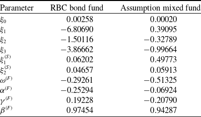
The model was estimated using monthly return data from October 2006 to October 2018 for the RBC Bond GIF Series 1 fund and from February 2002 to October 2018 for the Assumption/CI Harbour Growth & Income Fund Series A fund.
3.3. Risk factors and state space
Based on the mortality and market dynamics outlined in Sections 3.1 and 3.2, the variable annuity P&L can be decomposed as described in Section 2.1. The sources of risk are categorized into three main groups: term structure innovations
 $(z^{(r)}_{t,1}, z^{(r)}_{t,2}, z^{(r)}_{t,3})$
, equity innovations
$(z^{(r)}_{t,1}, z^{(r)}_{t,2}, z^{(r)}_{t,3})$
, equity innovations
 $(z^{(S)}_{t,1}, z^{(S)}_{t,2},z^{(F)}_{t})$
, and mortality innovations
$(z^{(S)}_{t,1}, z^{(S)}_{t,2},z^{(F)}_{t})$
, and mortality innovations
 $(\epsilon_t, \nu_t)$
. Therefore, the vector of shocks influencing the risk factors at time t is given by
$(\epsilon_t, \nu_t)$
. Therefore, the vector of shocks influencing the risk factors at time t is given by
 \begin{equation*} Y_t = \left( z^{(r)}_{t,1}, z^{(r)}_{t,2}, z^{(r)}_{t,3}, z^{(S)}_{t,1}, z^{(S)}_{t,2},z^{(F)}_{t}, \epsilon_t, \nu_t \right)^\top,\end{equation*}
where
 $\mathcal{S}_1=\{1,2,3\}$
,
$\mathcal{S}_1=\{1,2,3\}$
,
 $\mathcal{S}_2=\{4,5,6\}$
, and
$\mathcal{S}_2=\{4,5,6\}$
, and
 $\mathcal{S}_3=\{7,8\}$
. These shocks drive the evolution of the risk factor process, denoted by
$\mathcal{S}_3=\{7,8\}$
. These shocks drive the evolution of the risk factor process, denoted by
 \begin{equation*} X_t = \left( r^{(1)}_t, r^{(2)}_t, r^{(3)}_t, h^{(S)}_{t,1}, h^{(S)}_{t,2}, h^{(F)}_t, u_t, A_t \right)^\top,\end{equation*}
which includes term structure factors, equity volatilities, the mortality factor, and the account value.
The simulation of the risk process X and of associated innovations Y is conducted using Monte Carlo simulation under the physical probability measure
 $\mathbb{P}$
with dynamics outlined in Appendix D and Section 3.2.1. However, to calculate the value of the GMMB and GMWB variable annuities at any time t, the process is simulated under the risk-neutral probability measure
$\mathbb{P}$
with dynamics outlined in Appendix D and Section 3.2.1. However, to calculate the value of the GMMB and GMWB variable annuities at any time t, the process is simulated under the risk-neutral probability measure
 $\mathbb{Q}$
. The dynamics under
$\mathbb{Q}$
. The dynamics under
 $\mathbb{Q}$
are provided in Section 3.2.2. An overview of the Monte Carlo simulation methodology is provided in Appendix B.
$\mathbb{Q}$
are provided in Section 3.2.2. An overview of the Monte Carlo simulation methodology is provided in Appendix B.
4. Numerical experiments
4.1. Market settings for numerical experiments
We consider monthly trading periods, with market dynamics, risk factor processes, and cash flow specifications following the models and parameter estimates from Section 3 and Appendix D. All parameter values, including estimation details, are borrowed from Godin et al. (Reference Godin, Hamel, Gaillardetz and Ng2023).
Our analysis includes variable annuities with maturities of 20 years, that is, with
 $T=240$
months. It considers two funds: the Assumption mixed fund and the RBC bond fund, whose associated parameter estimates are described in Section 3.2.3. While the Assumption fund is mixed and contains both equity and fixed income investment, the RBC bond fund contains exclusively fixed income instruments. Fee rates are set to
$T=240$
months. It considers two funds: the Assumption mixed fund and the RBC bond fund, whose associated parameter estimates are described in Section 3.2.3. While the Assumption fund is mixed and contains both equity and fixed income investment, the RBC bond fund contains exclusively fixed income instruments. Fee rates are set to
 $\omega = 0.0286$
for the Assumption fund and to
$\omega = 0.0286$
for the Assumption fund and to
 $\omega = 0.0206$
for the RBC bond fund. Initial risk factor values correspond to filtered estimates as of October 31, 2018, with term structure factors given by
$\omega = 0.0206$
for the RBC bond fund. Initial risk factor values correspond to filtered estimates as of October 31, 2018, with term structure factors given by
 $r_0^{(1)} = -0.0690$
,
$r_0^{(1)} = -0.0690$
,
 $r_0^{(2)} = -0.0062$
, and
$r_0^{(2)} = -0.0062$
, and
 $r_0^{(3)} = 0.0940$
. Initial annualized volatilities are
$r_0^{(3)} = 0.0940$
. Initial annualized volatilities are
 $\sqrt{12h_0^{(S,1)}} = 0.1412$
for the S&P/TSX,
$\sqrt{12h_0^{(S,1)}} = 0.1412$
for the S&P/TSX,
 $\sqrt{12h_0^{(S,2)}} = 0.1785$
for the S&P 500,
$\sqrt{12h_0^{(S,2)}} = 0.1785$
for the S&P 500,
 $\sqrt{12h_0^{(F)}} = 0.0090$
for the RBC fund, and
$\sqrt{12h_0^{(F)}} = 0.0090$
for the RBC fund, and
 $\sqrt{12h_0^{(F)}} = 0.0416$
for the Assumption fund. For simulation purposes, all fund values and the account value are initialized to one, that is,
$\sqrt{12h_0^{(F)}} = 0.0416$
for the Assumption fund. For simulation purposes, all fund values and the account value are initialized to one, that is,
 $A_0 = F_0 = S_0^{(1)} = S_0^{(2)} = 1$
, with the guaranteed amount set to
$A_0 = F_0 = S_0^{(1)} = S_0^{(2)} = 1$
, with the guaranteed amount set to
 $G = 1$
in the GMMB case. For the GMWB case, which is not covered in Godin et al. (Reference Godin, Hamel, Gaillardetz and Ng2023), we set
$G = 1$
in the GMMB case. For the GMWB case, which is not covered in Godin et al. (Reference Godin, Hamel, Gaillardetz and Ng2023), we set
 $W=0.0154$
, which is the fair value leading to a null risk-neutral value of the guarantee (net of fees). The initial systemic mortality factor is
$W=0.0154$
, which is the fair value leading to a null risk-neutral value of the guarantee (net of fees). The initial systemic mortality factor is
 $u_0 = -64.73868$
. In all scenarios, the initial age of policyholders is set to 55 years.
$u_0 = -64.73868$
. In all scenarios, the initial age of policyholders is set to 55 years.
The hedging instruments consist of the risk-free asset and equity futures on both market indices, with each futures being rolled over every three months. Futures positions are closed at the end of each monthly period. The prices of the two equity futures maturing at time
 $t+n$
, observed at the beginning and end of the trading interval
$t+n$
, observed at the beginning and end of the trading interval
 $[t,t+1)$
, are given for
$[t,t+1)$
, are given for
 $j = 1, 2$
by the following formulas:
$j = 1, 2$
by the following formulas:
 \begin{align} I_{t,t+n}^{(j,b)}&=S_{t}^{(j)}\tilde{P}_{t,t+n}^{(S,j)}\, \mbox{ and } I_{t,t+n}^{(j,e)}=S_{t+1}^{(j)}\tilde{P}_{t+1,t+n}^{(S,j)}, \end{align}
 \begin{align} \tilde{P}_{t,t+n}^{(S,j)} &= \exp\left\{ \Lambda\sum_{i=1}^{3}m_{n,t}^{(i)}+\frac{\Lambda^{2}}{2}\sum_{i=1}^{3}\sum_{l=1}^{3}v_{n}^{(i,l)} \right\}, \end{align}
 \begin{align} m_{n,t}^{(i)} &= (r_{t}^{(i)}-\tilde{\mu}_{i})\left[ \frac{1-(1-\tilde{k}_{i})^{n}}{\tilde{k}_{i}} \right]+\tilde{\mu}_{i}n, \end{align}
 \begin{align} v_{n}^{(i,l)} &= \frac{\sigma_{i}}{\tilde{k}_{i}}\frac{\sigma_{l}}{\tilde{k}_{l}}\Gamma_{i,l}\left[ n- \frac{1-(1-\tilde{k}_{i})^{n}}{\tilde{k}_{i}} - \frac{1-(1-\tilde{k}_{l})^{n}}{\tilde{k}_{l}}+ \frac{1-(1-\tilde{k}_{i})^{n}(1-\tilde{k}_{l})^{n}}{1-(1-\tilde{k}_{i})(1-\tilde{k}_{l})}\right].\end{align}
The initial hedging portfolio value is
 $V_0 = 0$
. As such, the hedging portfolio value and the discounted gain and loss coincide:
$V_0 = 0$
. As such, the hedging portfolio value and the discounted gain and loss coincide:
 $V_t^\delta(V_0,X_{0}, Y_{1\,:\,t}) = G_t^\delta(X_{0}, Y_{1\,:\,t})$
.
$V_t^\delta(V_0,X_{0}, Y_{1\,:\,t}) = G_t^\delta(X_{0}, Y_{1\,:\,t})$
.
4.2. RL agent and CVaR network settings
This section provides the implementation details and hyperparameter choices for both the RL agent and the CVaR network.
4.2.1. RL agent parameters
RL agents are trained following the procedure outlined in Section 2.3, using a training set of 100,000 independently simulated paths. Training is conducted over 50 epochs for the GMMB and 100 epochs for the GMWB, using a mini-batch size of 1000 with learning rate parameters of 0.00005 and 0.00003, respectively. To enhance generalization, dropout regularization is applied with a probability parameter of
 $p=0.5$
. We do not conduct a formal hyperparameter tuning procedure, as ad hoc testing revealed that finding hyperparameters producing satisfactory performance through manual trial and error works reasonably well. The implementation is carried out in Python using TensorFlow, with neural network parameters initialized according to the method proposed by Glorot and Bengio (Reference Glorot and Bengio2010). We assess performance on a separate test set consisting of 1000 independent paths. A lower number of paths is considered to reduce the computational cost of evaluating the benchmark, which involves nested simulations that are computationally intensive and increase overall runtime. Table 4 summarizes the processing times from a representative experimental run on the GMWB policy, reporting the runtime requirements of each computational component.
$p=0.5$
. We do not conduct a formal hyperparameter tuning procedure, as ad hoc testing revealed that finding hyperparameters producing satisfactory performance through manual trial and error works reasonably well. The implementation is carried out in Python using TensorFlow, with neural network parameters initialized according to the method proposed by Glorot and Bengio (Reference Glorot and Bengio2010). We assess performance on a separate test set consisting of 1000 independent paths. A lower number of paths is considered to reduce the computational cost of evaluating the benchmark, which involves nested simulations that are computationally intensive and increase overall runtime. Table 4 summarizes the processing times from a representative experimental run on the GMWB policy, reporting the runtime requirements of each computational component.
Computation time for different components of the hedging frameworks, GMWB example.

The reported times correspond to a single experiment. Experiments and runtimes are measured on a compute node with 24 GB unified memory (shared CPU–GPU pool; capacity comparable to 24 GB system RAM but with higher effective utilization due to zero-copy access), under identical execution conditions. FFNN training uses 1 integrated GPU with 8 GPU cores. Total computation time aggregates all tasks for the corresponding hedging approach.
4.2.2. Conditional CVaR network parameters
The conditional CVaR network is trained on datapoints derived from 1000 paths sampled from the training set used for the RL agent. Assuming 240 time steps per path, this results in a total of 240,000 training datapoints. Training is carried out over 100 epochs with a mini-batch size of 2000 and an initial learning rate of 0.00001. As with the RL agent, dropout with a rate of
 $p=0.5$
is applied to enhance generalization and mitigate overfitting. The network is implemented in Python using TensorFlow, with weights initialized according to the Glorot scheme.
$p=0.5$
is applied to enhance generalization and mitigate overfitting. The network is implemented in Python using TensorFlow, with weights initialized according to the Glorot scheme.
4.3. Benchmarking framework
As a benchmark, we implement a delta hedging strategy that neutralizes the portfolio’s delta exposure using equity futures on both underlying indices. Since the pricing function
 $f_{t}$
has no closed-form solution and the delta depends on
$f_{t}$
has no closed-form solution and the delta depends on
 $f_{t}$
, we estimate the required Greeks using a forward finite difference approach based on Monte Carlo simulation with a sample size of 1000. To ensure the portfolio remains fully delta-neutral, futures positions are adjusted at each rebalancing time. Detailed formulas for delta hedging are provided in Appendix C.
$f_{t}$
, we estimate the required Greeks using a forward finite difference approach based on Monte Carlo simulation with a sample size of 1000. To ensure the portfolio remains fully delta-neutral, futures positions are adjusted at each rebalancing time. Detailed formulas for delta hedging are provided in Appendix C.
The comparison between our approach and the benchmark is based on the final terminal P&L of the insurer, which includes both these from the variable annuity and the hedging portfolio. It is defined as
Using the hedging decomposition scheme outlined in Section 2.1, the terminal P&L is decomposed into contributions from the various risk factors as follows:
where
 $\tilde{\mathcal{C}}^{(k)} = \mathcal{C}^{(k)} + \mathcal{H}^{(k)}_{\delta}$
for
$\tilde{\mathcal{C}}^{(k)} = \mathcal{C}^{(k)} + \mathcal{H}^{(k)}_{\delta}$
for
 $k = 1, 2, 3$
represent the net contribution of the term structure, the equity, and the mortality source of risk groups, respectively.
$k = 1, 2, 3$
represent the net contribution of the term structure, the equity, and the mortality source of risk groups, respectively.
 $\tilde{\Theta} = \Theta_{T} + \Theta_{T}^{V^\delta}$
represents the net contribution from the time passage risk factor. All contributions are based on the decompositions corresponding to Equations (2.4) and (2.6) for the variable annuity and hedging portfolio, respectively.
$\tilde{\Theta} = \Theta_{T} + \Theta_{T}^{V^\delta}$
represents the net contribution from the time passage risk factor. All contributions are based on the decompositions corresponding to Equations (2.4) and (2.6) for the variable annuity and hedging portfolio, respectively.
To assess the performance of the hedging strategies, we consider three distinct measures under the physical probability measure
 $\mathbb{P}$
: the expected final P&L,
$\mathbb{P}$
: the expected final P&L, ![]() , the variance of the final P&L,
, the variance of the final P&L, ![]() , and the CVaR at the
, and the CVaR at the
 $ 95\% $
confidence level,
$ 95\% $
confidence level, ![]() . We then perform risk allocation of these measures, which entails assessing what proportion of the risk measure values reported are caused by the various respective sources of risk groups. Obtaining the risk allocation for the various source of risk groups is essential to understand how each individual group contributes to the overall performance of the hedging strategy. The risk allocation for the k-th source of risk group is determined as follows:
. We then perform risk allocation of these measures, which entails assessing what proportion of the risk measure values reported are caused by the various respective sources of risk groups. Obtaining the risk allocation for the various source of risk groups is essential to understand how each individual group contributes to the overall performance of the hedging strategy. The risk allocation for the k-th source of risk group is determined as follows:
-
• For the expected value,
 $\mathcal{A}_{\tilde{\mathcal{C}}^{(k)}} = \mathbb{E}\big[\tilde{\mathcal{C}}^{(k)} \big]$
,
$\mathcal{A}_{\tilde{\mathcal{C}}^{(k)}} = \mathbb{E}\big[\tilde{\mathcal{C}}^{(k)} \big]$
, -
• For the variance,
$\mathcal{A}_{\tilde{\mathcal{C}}^{(k)}} = \text{Cov}\left(\tilde{\mathcal{C}}^{(k)}, \sum_{i=1}^{3} \tilde{\mathcal{C}}^{(i)} + \tilde{\Theta} \right)$
, -
• For the CVaR,
.

4.4. Benchmarking hedging strategies
4.4.1. Benchmarking with delta hedging
We begin our analysis by evaluating the hedging performance of two strategies: delta hedging and targeted risk hedging with equity risk being chosen for mitigation, that is,
 $\mathcal{T}=2$
, which entails targeting sources of risk
$\mathcal{T}=2$
, which entails targeting sources of risk
 $(z^{(S)}_{t,1}, z^{(S)}_{t,2},z^{(F)}_{t})$
. To assess the robustness of our approach, we conduct this analysis on the GMMB and GMWB contracts using the two underlying funds: the Assumption mixed fund and the RBC bond fund.
$(z^{(S)}_{t,1}, z^{(S)}_{t,2},z^{(F)}_{t})$
. To assess the robustness of our approach, we conduct this analysis on the GMMB and GMWB contracts using the two underlying funds: the Assumption mixed fund and the RBC bond fund.
We first present the results for the GMMB contract. The numerical results presented in Table 5 display the impact of hedging on risk for the two underlying funds. The various columns provide the performance metrics associated with optimal allocations for three different insurer portfolios without hedging, with delta hedging, and with targeted risk hedging.
Total risk allocation of 20-year GMMB variable annuities, with and without hedging.

Results are based on 1000 out-of-sample paths. The hedged risk is the equity risk component of a GMMB variable annuity with a maturity of
 $T = 240$
months, with hedging portfolios rebalanced monthly. The decomposition into contributions from the various source of risk groups is performed on the terminal portfolio value following the methodology outlined in Section 2.1. The CVaR is applied to the negative P&L to capture tail risk.
$T = 240$
months, with hedging portfolios rebalanced monthly. The decomposition into contributions from the various source of risk groups is performed on the terminal portfolio value following the methodology outlined in Section 2.1. The CVaR is applied to the negative P&L to capture tail risk.
Our numerical results in Table 5 reveal that delta hedging fails to effectively mitigate long-term risk and, in some cases, even exacerbates it. While the total variance remains nearly unchanged for the Assumption mixed fund, it increases by more than 50% for the RBC bond fund, rising from 0.00104 to 0.00162 when comparing the “No hedging” and “Delta hedging” columns. Additionally, delta hedging significantly amplifies long-term tail risk, with the CVaR rising from 0.15885 to 0.23020 for the Assumption mixed fund and from 0.09393 to 0.14004 for the RBC bond fund, as seen in the corresponding columns. This can partially be explained by the fact that the CVaR is translation invariant, and that delta hedging deteriorates total expected gains as seen in the table.
In contrast, the DTH approach successfully reduces both the variance and the CVaR, demonstrating its effectiveness in managing risk regardless of the underlying fund. When comparing the “No hedging” and “DTH” columns, total variance decreases from 0.00686 to 0.00243 for the Assumption mixed fund and from 0.00104 to 0.00086 for the RBC bond fund. Similarly, the global CVaR exposure declines from 0.15885 to 0.06014 for the Assumption mixed fund and from 0.09393 to 0.07489 for the RBC bond fund. These results highlight the superior risk management capabilities of DTH compared to delta hedging.
Additionally, our approach effectively neutralizes the equity risk component, resulting in a CVaR allocation of
 $-0.03532$
under the “DTH” column for the Assumption mixed fund. Negative values for the a CVaR allocation component indicate that such component has an offsetting effect on the CVaR, helping reducing it. In addition, the overall CVaR is reduced by 0.09871, computed as the difference between the total CVaR in the “No hedging” scenario (0.15885) and the “DTH” scenario (0.06014). This reduction closely aligns with the original equity risk allocation (0.09367), confirming the strategy’s accuracy in isolating and mitigating the targeted risk source group. Furthermore, our targeted risk approach does not cause an increase in risk allocations for any of the other source of risk groups (except for the passage of time); both variance and CVaR allocations to any component other than equity risk decrease.
$-0.03532$
under the “DTH” column for the Assumption mixed fund. Negative values for the a CVaR allocation component indicate that such component has an offsetting effect on the CVaR, helping reducing it. In addition, the overall CVaR is reduced by 0.09871, computed as the difference between the total CVaR in the “No hedging” scenario (0.15885) and the “DTH” scenario (0.06014). This reduction closely aligns with the original equity risk allocation (0.09367), confirming the strategy’s accuracy in isolating and mitigating the targeted risk source group. Furthermore, our targeted risk approach does not cause an increase in risk allocations for any of the other source of risk groups (except for the passage of time); both variance and CVaR allocations to any component other than equity risk decrease.
Similarly, when considering the RBC bond fund, the reduction in CVaR yields a value of 0.01904, which closely aligns with the CVaR allocation of the equity component without hedging (0.02802). At the same time, the other sources of risk remain mostly unaffected.
In addition, our hedging framework consistently yields higher expected P&L than delta hedging, highlighting its superior overall performance. While hedging strategies typically reduce profitability by the end of the hedging period, our approach avoids penalizing gains from the targeted sources of risk. As a result, the expected contribution from this targeted component tends to increase. On the other hand, delta hedging fails to effectively hedge the equity component, despite being designed to align with it. As explained in Godin et al. (Reference Godin, Hamel, Gaillardetz and Ng2023), the hedge’s failure can be attributed to the mismatch between the equity futures used for hedging and the actual underlying risk, a phenomenon known as basis risk. This occurs when the hedging instrument (equity futures) does not perfectly correlate with the risk exposure of the GMMB product. As a result, delta hedging tends to over-hedge the position. This over-hedging not only leads to incomplete risk mitigation, but it also dampens profitability, as the strategy relies on large positions providing high short exposure to the equity risk premium. These shortcomings are clearly reflected in the lower expected P&L reported in Table 5.
Results for the GMWB contracts are reported in Table 6. The table presents the same set of performance metrics as for the GMMB, across the two underlying funds and the three hedging strategies. The overall conclusions remain consistent: while delta hedging provides long-term risk reduction for the GMWB (except for the CVaR
 $_{95\%}$
metric when the underlying fund is the RBC bond fund), the equity risk component still remains substantial after hedging. In contrast, the targeted hedging framework succeeds in substantially lowering global risk exposure while neutralizing most of the targeted equity risk. This is achieved while simultaneously improving profitability in comparison to delta hedging. Thus, the superiority of the targeted hedging approach is again evident. Given that conclusions are qualitatively similar for the GMMB and GMWB products, we focus on the GMMB contract in the remainder of the paper.
$_{95\%}$
metric when the underlying fund is the RBC bond fund), the equity risk component still remains substantial after hedging. In contrast, the targeted hedging framework succeeds in substantially lowering global risk exposure while neutralizing most of the targeted equity risk. This is achieved while simultaneously improving profitability in comparison to delta hedging. Thus, the superiority of the targeted hedging approach is again evident. Given that conclusions are qualitatively similar for the GMMB and GMWB products, we focus on the GMMB contract in the remainder of the paper.
Total risk allocation of GMWB variable annuities, with and without hedging.

Results are based on 1000 out-of-sample paths. The hedged risk is the equity risk component of a GMWB variable annuity, with hedging portfolios rebalanced monthly. The decomposition into contributions from the various source of risk groups is performed on the terminal portfolio value following the methodology outlined in Section 2.1. The CVaR is applied to the negative P&L to capture tail risk.
Total risk allocation across different RL settings for a GMMB on the assumption mixed fund.

Results are based on 1000 out-of-sample paths. The hedged is the equity component of a GMMB variable annuity with a maturity of
 $T = 240$
months, with hedging portfolios rebalanced monthly. The decomposition into contributions from the various source of risk groups is performed on the terminal portfolio value following the methodology outlined in Section 2.1. The CVaR is applied to the negative P&L to capture tail risk.
$T = 240$
months, with hedging portfolios rebalanced monthly. The decomposition into contributions from the various source of risk groups is performed on the terminal portfolio value following the methodology outlined in Section 2.1. The CVaR is applied to the negative P&L to capture tail risk.
Impact of the local penalty on total risk allocation for a GMMB on the assumption mixed fund.

Results are based on 1000 out-of-sample paths. The hedged is the equity component of a variable annuity with a maturity of
 $T = 240$
months, with hedging portfolios rebalanced monthly. The decomposition into contributions from the various sources of risk groups is performed on the terminal portfolio value following the methodology outlined in Section 2.1. The CVaR is applied to the negative P&L to capture tail risk. The objective functions for the RL approach are defined as described in Section 2.3 and
$T = 240$
months, with hedging portfolios rebalanced monthly. The decomposition into contributions from the various sources of risk groups is performed on the terminal portfolio value following the methodology outlined in Section 2.1. The CVaR is applied to the negative P&L to capture tail risk. The objective functions for the RL approach are defined as described in Section 2.3 and
 $L^{*}\left(\theta\right)=\| (\mathcal{H}^{(\mathcal{T})}_{\tilde\delta_{\theta}} + \mathcal{C}^{(\mathcal{T})})\unicode{x1D7D9}_{\{\mathcal{H}^{(\mathcal{T})}_{\tilde\delta_{\theta}} + \mathcal{C}^{(\mathcal{T})} \lt 0\}} \|_{\mathcal{L}^{2}}$
.
$L^{*}\left(\theta\right)=\| (\mathcal{H}^{(\mathcal{T})}_{\tilde\delta_{\theta}} + \mathcal{C}^{(\mathcal{T})})\unicode{x1D7D9}_{\{\mathcal{H}^{(\mathcal{T})}_{\tilde\delta_{\theta}} + \mathcal{C}^{(\mathcal{T})} \lt 0\}} \|_{\mathcal{L}^{2}}$
.
4.4.2. Benchmarking with deep hedging
We continue our analysis by benchmarking our framework against the traditional deep hedging approach, which does not target a specific component of risk and hedges entire cash flows. For consistency, we use the same network architecture and parameters described in Section 4.2.1. However, the objective function in this baseline aims to minimize the losses of final discounted terminal P&L of the insurer, ![]() . Such objective function is the semi-mean squared error (SMSE), defined as
. Such objective function is the semi-mean squared error (SMSE), defined as
For illustration, we present results using the Assumption mixed fund as the underlying asset. Detailed outcomes for other underlying assets are omitted for brevity but are conceptually similar. Table 7 summarizes the optimal hedging performance metrics, with the “No hedging” case serving as a baseline.
Our numerical results demonstrate that deep hedging improves risk management by reducing allocations for both variance and CVaR compared to the no-hedging scenario. Surprisingly, these reductions are less pronounced than those achieved by our approach despite performance metrics being reported on the full ![]() . This can be partially explained by the use of the semi-quadratic objective function by the deep hedging agent, which does not fully align with the variance and CVaR performance metrics reported. Our results indicate that the reductions in risk allocations from our targeted risk approach are not solely attributable to the use of a multistage-optimal strategy such as deep hedging framework; rather, the use of risk targeting changes the structure of the hedging portfolio and provides incremental benefits. Specifically, as observed in the CVaR risk measure allocations, deep hedging does not fully eliminate the contribution from the equity component. While deep hedging reduces equity risk from 0.09367 (in the “No hedging” scenario) to 0.07378 (in the “Deep hedging” scenario), our approach completely neutralizes this risk allocation, resulting in a value of
. This can be partially explained by the use of the semi-quadratic objective function by the deep hedging agent, which does not fully align with the variance and CVaR performance metrics reported. Our results indicate that the reductions in risk allocations from our targeted risk approach are not solely attributable to the use of a multistage-optimal strategy such as deep hedging framework; rather, the use of risk targeting changes the structure of the hedging portfolio and provides incremental benefits. Specifically, as observed in the CVaR risk measure allocations, deep hedging does not fully eliminate the contribution from the equity component. While deep hedging reduces equity risk from 0.09367 (in the “No hedging” scenario) to 0.07378 (in the “Deep hedging” scenario), our approach completely neutralizes this risk allocation, resulting in a value of
 $-0.03532$
. This highlights the advantages of our targeted risk hedging framework, which effectively mitigates the targeted risk component.
$-0.03532$
. This highlights the advantages of our targeted risk hedging framework, which effectively mitigates the targeted risk component.
Additionally, it is important to note that the SMSE of the DTH approach is 0.00032, which is slightly higher than the 0.00008 observed with deep hedging. This difference reflects the trade-off inherent in our approach, as deep hedging is specifically designed to minimize overall SMSE through its objective function.
4.5. Impact of local risk penalization on performance
In this section, we analyze the impact of local risk penalization on performance. This evaluation allows to assess the effect of incorporating the penalty term from Equation (2.10) into the objective function. For illustration, we only present results for the Assumption mixed fund underlying asset.
Table 8 presents the optimal hedging performance metrics applied to the total discounted P&L, ![]() . The “No hedging” case serves as a baseline. The table also includes results for two RL-based hedging strategies, both labeled “RL hedging”; the column
. The “No hedging” case serves as a baseline. The table also includes results for two RL-based hedging strategies, both labeled “RL hedging”; the column
 $L\left(\theta^{(1)}\right)$
presents results when a weight of
$L\left(\theta^{(1)}\right)$
presents results when a weight of
 $p=0$
is assigned to the local risk component of the objective function, while the column
$p=0$
is assigned to the local risk component of the objective function, while the column
 $\mathcal{O}_{\alpha}^{p}(\theta^{(1)})$
exhibits results for the full objective function (2.11) with
$\mathcal{O}_{\alpha}^{p}(\theta^{(1)})$
exhibits results for the full objective function (2.11) with
 $p=1/T$
.
$p=1/T$
.
Numerical results confirm that both RL configurations effectively manage risk with respect to the cumulative P&L, as evidenced by the allocation metrics. Both the CVaR and variance are significantly lower compared to the values achieved without hedging. In particular, the risk associated with equity exposure is well managed, with allocations being close to zero for the variance and below zero for the CVaR.
Regarding the RL configurations, we observe that the RL hedging strategy with local risk penalization, whose performance is reported in column
 $\mathcal{O}_{\alpha}^{p}(\theta)$
, yields the lowest variance and CVaR values for the total risk encompassing all risk components. While local risk penalization is primarily aimed at improving short-term risk control, our results indicate that it also maintains or improves global risk metrics. This outcome can be attributed to the regularizing effect of local penalization, which discourages extreme fluctuations in the P&L.
$\mathcal{O}_{\alpha}^{p}(\theta)$
, yields the lowest variance and CVaR values for the total risk encompassing all risk components. While local risk penalization is primarily aimed at improving short-term risk control, our results indicate that it also maintains or improves global risk metrics. This outcome can be attributed to the regularizing effect of local penalization, which discourages extreme fluctuations in the P&L.
Furthermore, risk allocations for the various components are all reduced by the inclusion of the penalty term in the objective function; except for the equity risk component of the CVaR, all allocation values for both the variance and CVaR are lower in the
 $\mathcal{O}_{\alpha}^{p}(\theta)$
than in the
$\mathcal{O}_{\alpha}^{p}(\theta)$
than in the
 $L\left(\theta^{(1)}\right)$
column.
$L\left(\theta^{(1)}\right)$
column.
To evaluate the effect of local risk penalization throughout the hedging horizon, we analyze for various t’s the CVaR of the time-t cumulative P&L defined as
see Section 4.6 for the definition of
 $\text{NGL}_{t}^{\delta}$
.
$\text{NGL}_{t}^{\delta}$
.
Figure 1 compares the 95%-level CVaR of ![]() for four hedging strategies: no hedging, the delta hedging benchmark, an RL agent optimized under the objective function
for four hedging strategies: no hedging, the delta hedging benchmark, an RL agent optimized under the objective function
 $L\left(\theta\right)$
(which excludes local risk penalization), and an RL agent trained with the penalization term included, using the objective function
$L\left(\theta\right)$
(which excludes local risk penalization), and an RL agent trained with the penalization term included, using the objective function
 $\mathcal{O}_{\alpha}^{p}(\theta)$
.
$\mathcal{O}_{\alpha}^{p}(\theta)$
.
CVaR of cumulative gains and losses over the hedging horizon. Results are based on 1000 out-of-sample paths. The hedged is the equity component of a GMMB variable annuity with a maturity of
 $T = 240$
months, rebalanced monthly under the assumed fund dynamics. The CVaR is computed at a 95% confidence level. In the local penalization scenario, the penalization parameter is set to
$T = 240$
months, rebalanced monthly under the assumed fund dynamics. The CVaR is computed at a 95% confidence level. In the local penalization scenario, the penalization parameter is set to
 $\frac{1}{T}$
. The CVaR is applied to the negative P&L to capture tail risk.
$\frac{1}{T}$
. The CVaR is applied to the negative P&L to capture tail risk.

Our findings show that both RL agents effectively reduce CVaR throughout the hedging period, as indicated by the yellow and green curves representing the CVaR of the RL strategies, which are lower than the blue curve for the variable annuity without hedging. However, only the agent incorporating local risk penalization outperforms the benchmark over the whole hedging horizon, as shown by the green curve, which exhibits lower values than the red curve associated with delta hedging. This highlights the benefit of this additional control in enhancing risk management.
Together with the results presented in Table 8, these findings demonstrate that local risk penalization enhances risk control not only at the end of the hedging period but also throughout its duration.
4.6. Local contribution of risk factors
In this section, we analyze the local impact of different sources of risk groups by decomposing the period-by-period net gains
 $\text{NGL}_{t}^{\delta}$
defined in (2.9), where the net loss is decomposed in the same manner as the terminal P&L, attributing it to four distinct source of risk groups (i.e., equity, interest rates, mortality, and passage of time), as described in Equation (4.5). Specifically, the net gain decomposition for the i-th simulated path at time t is given by
$\text{NGL}_{t}^{\delta}$
defined in (2.9), where the net loss is decomposed in the same manner as the terminal P&L, attributing it to four distinct source of risk groups (i.e., equity, interest rates, mortality, and passage of time), as described in Equation (4.5). Specifically, the net gain decomposition for the i-th simulated path at time t is given by
 \begin{equation*} \text{NGL}_{t}^{(\delta,i)} = \sum_{k=1}^{3} \tilde{\mathcal{C}}_{t}^{(\text{k},i)} + \tilde{\Theta}^{(i)}_t,\end{equation*}
where
 $\tilde{\mathcal{C}}^{(k,i)}_t$
for
$\tilde{\mathcal{C}}^{(k,i)}_t$
for
 $k = 1, 2, 3$
represents the contribution from interest rate risk, equity risk, and mortality risk, respectively.
$k = 1, 2, 3$
represents the contribution from interest rate risk, equity risk, and mortality risk, respectively.
 $\tilde{\Theta}^{(i)}_t$
represents the contribution from the time passage risk factor. The purpose of examining the local net losses is to assess the contribution of individual source of risk groups and evaluate the impact of hedging on a period-by-period basis.
$\tilde{\Theta}^{(i)}_t$
represents the contribution from the time passage risk factor. The purpose of examining the local net losses is to assess the contribution of individual source of risk groups and evaluate the impact of hedging on a period-by-period basis.
For illustration, we consider a GMMB variable annuity, where the underlying fund following the dynamics of the Assumption mixed fund. This case is chosen for its illustrative value, as the results remain consistent across different maturities and underlying fund choices.
Our analysis study the distribution and the average period-by-period contribution of each risk source. The average contributions are defined as
 \begin{equation*} \widehat{\mathcal{C}}^{(k)}_t=\frac{1}{1000}\sum_{i=1}^{1000}\tilde{\mathcal{C}}^{(k,i)}_t, \, \text{for } k = 1, 2, 3;\, \text{ and } \widehat{\Theta}_t =\frac{1}{1000}\sum_{i=1}^{1000} \tilde{\Theta}_t^{(i)}.\end{equation*}
Figure 2 provides average net contributions
 $\widehat{\Theta}_t$
and
$\widehat{\Theta}_t$
and
 $\widehat{\mathcal{C}}^{(k)}_t$
versus t, which are given by the full lines. Shaded areas in the figure represent the interquartile range of net contributions for each t. The Figure 2 is organized into three panels. Panel A shows the net contributions in the absence of hedging, while Panels B and C illustrate these for delta hedging and targeted risk hedging, respectively.
$\widehat{\mathcal{C}}^{(k)}_t$
versus t, which are given by the full lines. Shaded areas in the figure represent the interquartile range of net contributions for each t. The Figure 2 is organized into three panels. Panel A shows the net contributions in the absence of hedging, while Panels B and C illustrate these for delta hedging and targeted risk hedging, respectively.
Average local contribution of the risk factors to gains and losses. Results are based on 1000 out-of-sample paths. The hedged target is the equity component of a variable annuity on the Assumption fund with a maturity of
 $T = 240$
months. Rebalancing is performed monthly. The risk factor decomposition is computed as described in Section 2.1. The shaded confidence bands represent the interquartile range, spanning from the 25th to the 75th percentile.
$T = 240$
months. Rebalancing is performed monthly. The risk factor decomposition is computed as described in Section 2.1. The shaded confidence bands represent the interquartile range, spanning from the 25th to the 75th percentile.

As shown in Figure 2, the source of risk groups exhibits varying impacts throughout the life of the contract, consistently with the findings of Godin et al. (Reference Godin, Hamel, Gaillardetz and Ng2023). The average contribution of mortality risk remains close to zero over most of the hedging period, indicating a relatively minor influence on net losses compared to other sources of risk. This limited impact is partly due to the fact that our framework models only systematic mortality risk, excluding idiosyncratic mortality fluctuations that could introduce greater variability at the individual level. Nonetheless, a positive contribution is observed near maturity, which is expected given that the contract’s payout structure places increasing weight on mortality outcomes as the contract nears maturity.
In contrast, the equity and interest rate factors become more volatile, with their mean exhibiting a greater deviation from zero. Since Figure 2 displays gains, lower mean values suggest that these sources of risk are contributing more to losses. Notably, the interest rate risk contribution decays early in the horizon, whereas the equity risk contribution starts to decline only a few months before maturity. This behavior can be explained by Godin et al. (Reference Godin, Hamel, Gaillardetz and Ng2023), who note that, as maturity nears, only a small portion of fees remain to be collected, and the sources of risk primarily contribute to the potential for benefit appreciation. Therefore, there is limited upside risk associated with potentially higher fees charged to policyholders. Thus, shocks on risk factors are more likely to cause losses, especially due to the convexity of the value of options embedded in the contract with respect to equity rate shocks. The negative contribution from the interest rate factor emerges earlier in the horizon, due to the impact of interest rates on discount factors; impacts of interest rate movements in early stages are compounded over multiple time periods and influence the present value of a larger set of cash flows.
In terms of the effect of hedging, we observe that gains and losses under the DTH strategy primarily impact the equity component. This is evident in Panel C, where the average contributions of the non-equity source of risk groups remain consistent with those in Panels A and B. However, the equity component displays a distinct pattern; its curve, in blue, shows higher values and a noticeable positive deviation from zero, indicating that DTH adjusts hedging position to increase the upside risk potential of equity risk. Such findings are consistent with the nature of targeted risk hedging and the design of its objective function, which specifically penalizes negative contributions from the equity risk component that is targeted, while aiming to minimize the impact of the hedging portfolio on contributions of other sources of risk.
5. Conclusion
We present a deep RL framework designed to optimize the hedging of specific components of risks that are targeted when performing the risk management of complex financial instruments driven by multiple risk factors. Our methodology incorporates Shapley decompositions to decompose contract cash flows into contributions from various source of risk groups, providing a detailed attribution of profits and losses to the various risk drivers. This tailored approach provides an efficient solution for managing complex hedging scenarios, particularly for instruments like variable annuities, where multiple, often interacting, risks must be addressed simultaneously.
Additionally, our approach incorporates local risk management through a novel auxiliary neural network. This auxiliary component effectively penalizes extreme values of the one-period P&L, contributing to more stable outcomes, enhancing the robustness of the hedging strategy, and reducing capital requirements to protect against short-term risk.
Through numerical experiments relying on models calibrated with real market data, we demonstrate that the proposed RL approach significantly outperforms the traditional delta hedging method. The results show marked improvements in reducing targeted risks, while leading to limited impacts on risk allocations to sources of risk that are not targeted. As a consequence, the RL-based strategy is able to substantially reduce the variance and tail risk of the overall risk exposure. Furthermore, the RL approach leads to higher profitability than delta-hedging, adequately adjusting hedge ratios to the presence of basis risk.
Our results show that DTH offers distinct advantages over conventional deep hedging by fully neutralizing the targeted risk. While deep hedging considers interactions between risks, our approach goes further by specifically isolating the sources of risk, ensuring that the targeted risk is mitigated without affecting other risk factors. This distinction is particularly valuable in scenarios where agents are tasked with hedging a specific risk while leaving others unaffected.
Furthermore, DTH is able to shift the targeted risks contribution’s distribution throughout most of the hedging period, enhancing upside risk potential for such source of risk. This indicates that our approach effectively mitigates adverse impacts from the targeted source of risk while generating limited impact to contributions from other sources of risk, in accordance with the design of our objective function.
Funding statement
This work is supported by a grant from the Canadian Institute of Actuaries. Godin is funded by NSERC (RGPIN-2024-04593).
Competing interests
The authors declare none.
A. Details for the MSGD training approach
A.1. Training approach for the hedging agent network
The MSGD method estimates the penalty function
 $\mathcal{O}_{\alpha}^{p}(\theta)$
using Shapley-type decompositions of the P&L for both the insurance contract and the hedging portfolio. Let
$\mathcal{O}_{\alpha}^{p}(\theta)$
using Shapley-type decompositions of the P&L for both the insurance contract and the hedging portfolio. Let
 $\mathbb{D}$
be the power set of
$\mathbb{D}$
be the power set of
 $\{1,2,3\}$
. We consider a sample
$\{1,2,3\}$
. We consider a sample
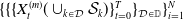 $\{\{\{X^{(m)}_{t}(\cup_{k\in \mathcal{D}}\mathcal{S}_k)\}_{t=0}^{T}\}_{\mathcal{D} \in \mathbb{D}}\}_{i=1}^{N}$
, where
$\{\{\{X^{(m)}_{t}(\cup_{k\in \mathcal{D}}\mathcal{S}_k)\}_{t=0}^{T}\}_{\mathcal{D} \in \mathbb{D}}\}_{i=1}^{N}$
, where
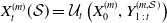 $X_{t}^{(m)}(\mathcal{S}) = \mathcal{U}_{t}\left(X_{0}^{(m)}, Y_{1\,:\,t}^{(m,\mathcal{S})}\right)$
represents the time-t risk factor values for n-th path under the set of shocked sources of risk group
$X_{t}^{(m)}(\mathcal{S}) = \mathcal{U}_{t}\left(X_{0}^{(m)}, Y_{1\,:\,t}^{(m,\mathcal{S})}\right)$
represents the time-t risk factor values for n-th path under the set of shocked sources of risk group
 $\mathcal{S}$
. This sample is divided into
$\mathcal{S}$
. This sample is divided into
 $N_{\text{batch}}$
batches, where each batch is defined as
$N_{\text{batch}}$
batches, where each batch is defined as
 $\mathbb{B}_{i} = \{\{\{X^{((i-1) N_{\text{batch}}+n)}_{t}(\cup_{k\in \mathcal{D}}\mathcal{S}_k)\}_{t=0}^{T}\}_{\mathcal{D} \in \mathbb{D}}\}_{n=1}^{B_{\text{batch}}}$
, with
$\mathbb{B}_{i} = \{\{\{X^{((i-1) N_{\text{batch}}+n)}_{t}(\cup_{k\in \mathcal{D}}\mathcal{S}_k)\}_{t=0}^{T}\}_{\mathcal{D} \in \mathbb{D}}\}_{n=1}^{B_{\text{batch}}}$
, with
 $N=B_{\text{batch}}N_{\text{batch}}$
. Each batch is then used to update the current policy parameters,
$N=B_{\text{batch}}N_{\text{batch}}$
. Each batch is then used to update the current policy parameters,
 $\theta_{i}^{(1)}$
and
$\theta_{i}^{(1)}$
and
 $\eta_{i}^{(1)}$
.
$\eta_{i}^{(1)}$
.
MSGD training approach for a single epoch.

CVaR estimation, stochastic-on-stochastic approach.

A.2. Training approach for the CVaR estimation network
The MSGD training approach detailed in Appendix A.1 is used to train a neural network that estimates the CVaR of the net cash flow resulting from each time-t rebalancing decision, denoted by
 $\text{CVaR}_{\alpha}^{(i,n,t)}$
. The estimator is modeled as a feedforward neural network,
$\text{CVaR}_{\alpha}^{(i,n,t)}$
. The estimator is modeled as a feedforward neural network,
 $F_{\theta^{(2)}}$
, which takes as input the vector
$F_{\theta^{(2)}}$
, which takes as input the vector
 $(\delta_{t+1}^{(i,n)}, X_t^{(i,n)}, t)$
and approximates the CVaR through the mapping
$(\delta_{t+1}^{(i,n)}, X_t^{(i,n)}, t)$
and approximates the CVaR through the mapping
 \begin{equation*} \text{CVaR}_{\alpha}^{(i,n,t)} = F_{\theta^{(2)}}\big( \delta_{t+1}^{(i,n)}, X_t^{(i,n)}, t\big).\end{equation*}
The neural network
 $F_{\theta^{(2)}}$
is trained offline following the stochastic-on-stochastic scheme described in Algorithm 2, where stochastic actions are sampled directly rather than relying on a fully optimized policy. The training process uses the same settings as in Appendix A.1, with the distinction that the sample of paths is restricted to their evolution under the influence of all risk factors, represented as
$F_{\theta^{(2)}}$
is trained offline following the stochastic-on-stochastic scheme described in Algorithm 2, where stochastic actions are sampled directly rather than relying on a fully optimized policy. The training process uses the same settings as in Appendix A.1, with the distinction that the sample of paths is restricted to their evolution under the influence of all risk factors, represented as
 $\{\{X^{(m)}_{t}\}_{t=0}^{T} \}_{m=1}^{N}$
. Once trained,
$\{\{X^{(m)}_{t}\}_{t=0}^{T} \}_{m=1}^{N}$
. Once trained,
 $F_{\hat\theta^{(2)}}$
with optimized parameters
$F_{\hat\theta^{(2)}}$
with optimized parameters
 $\hat\theta^{(2)}$
is used as a fixed function in Algorithm 1.
$\hat\theta^{(2)}$
is used as a fixed function in Algorithm 1.
B. Monte Carlo simulation methodology
This appendix provides an overview of the Monte Carlo simulation methodology employed in our framework. It outlines the key steps involved in simulating risk factors.
Monte Carlo simulation.

C. Delta hedging details
The delta of the overall portfolio is neutralized by adjusting the futures position,
 \begin{equation} \Delta_{t+1}^{(S,j)} = - \frac{\Psi^{(\text{guar}, A)}_t A_t \xi_j^{(S)}}{S^{(j)}_t} \cdot \frac{1}{\tilde{P}_{t,t+n}^{(S,j)}},\end{equation}
where
 \begin{equation} \Psi^{(\text{guar}, A)}_t = \frac{\partial f}{\partial A_{t}}(t,X_{t}).\end{equation}
Since no closed-form solution exists for the pricing function f, the Greek associated with the account value is estimated using a forward finite difference approach based on Monte Carlo simulations,
 \begin{equation} \frac{\partial f}{\partial A_{t}}(X_{t})\approx \frac{\hat{f}(t,X_{t}+\unicode{x1D7D9}_{A_t}\epsilon)-\hat{f}(t,X_{t})}{\epsilon},\end{equation}
where
 $\epsilon=0.01$
and
$\epsilon=0.01$
and
 $\unicode{x1D7D9}_{A}$
is an unit vector that takes the value 1 only at the position corresponding to the
$\unicode{x1D7D9}_{A}$
is an unit vector that takes the value 1 only at the position corresponding to the
 $A_t$
component in
$A_t$
component in
 $X_t$
. Additional details on the formulas and estimation process can be found in Godin et al. (Reference Godin, Hamel, Gaillardetz and Ng2023).
$X_t$
. Additional details on the formulas and estimation process can be found in Godin et al. (Reference Godin, Hamel, Gaillardetz and Ng2023).
D. Formulation of variable annuities and market dynamics
The policy account value
 $A_t$
evolves as
$A_t$
evolves as
 \begin{equation}A_t = (A_{t-1} -W) \frac{F_t}{F_{t-1}} (1 - \omega), \quad t = 1, \dots, T,\end{equation}
where
 $F_t$
is the value of the underlying fund, W is the withdrawn amount and
$F_t$
is the value of the underlying fund, W is the withdrawn amount and
 $\omega$
is the insurer’s periodic fee rate.
$\omega$
is the insurer’s periodic fee rate.
Fees are charged at the end of the period for all policyholders active at the beginning of the period:
 \begin{equation} \text{Fee}_t = { }_{t-1}{a}_{x}\, \omega\, (A_{t-1} -W) \frac{F_t}{F_{t-1}}, \quad t = 1, \dots, T,\end{equation}
where
 ${ }_{t-1}{a}_{x}$
is the proportion of active policyholders at time
${ }_{t-1}{a}_{x}$
is the proportion of active policyholders at time
 $t-1$
with the associated account value
$t-1$
with the associated account value
 $A_{t-1}$
.
$A_{t-1}$
.
The proportion of active policyholders at time t, denoted by
 ${}_{t}{a}_{x}$
, starts with an initial value of
${}_{t}{a}_{x}$
, starts with an initial value of
 ${ }_{0}{a}_{x} = 1$
and evolves according to
${ }_{0}{a}_{x} = 1$
and evolves according to
 \begin{equation}{}_{t}{a}_{x} = { }_{t-1}{a}_{x} \frac{{}_{t}{p}_{x}}{{ }_{t-1}{p}_{x}} (1 - \mathcal{L}(m_{t-1})), \quad t = 1, \dots, T,\end{equation}
where
 $\mathcal{L}(m_{t-1})$
is the lapse probability and
$\mathcal{L}(m_{t-1})$
is the lapse probability and
 ${}_{t}{p}_{x}$
denotes the probability that the policyholder survives at least t periods after time 0. For the GMMB policy, the lapse probability is function of the moneyness ratio
${}_{t}{p}_{x}$
denotes the probability that the policyholder survives at least t periods after time 0. For the GMMB policy, the lapse probability is function of the moneyness ratio
 $m_{t-1} = \frac{A_{t-1}}{G}$
, whereas the lapse function assumed to be constant (
$m_{t-1} = \frac{A_{t-1}}{G}$
, whereas the lapse function assumed to be constant (
 $\mathcal{L}(m_t)\equiv 0.06$
) for the GMWB policy. The lapse function for GMMB policies is taken from Augustyniak et al. (Reference Augustyniak, Godin and Hamel2021). The lapse rate
$\mathcal{L}(m_t)\equiv 0.06$
) for the GMWB policy. The lapse function for GMMB policies is taken from Augustyniak et al. (Reference Augustyniak, Godin and Hamel2021). The lapse rate
 $\mathcal{L}$
is given by
$\mathcal{L}$
is given by
 \begin{equation} \mathcal{L}(m_t) = 1 - \left(1 - \mathcal{L}^{\text{ann}}(m_t)\right)^{\Lambda}, \quad \mathcal{L}^{\text{ann}}(m_t) = \max \left( \gamma_1, \min \left( \gamma_2, \gamma_1 + \gamma_2\frac{(\kappa_2 - \kappa_1)}{m_t - \kappa_1} \right) \right), \end{equation}
where
 $\gamma_1$
and
$\gamma_1$
and
 $\gamma_2$
are boundary values, and
$\gamma_2$
are boundary values, and
 $\kappa_1$
and
$\kappa_1$
and
 $\kappa_2$
adjust the lapse function shape based on moneyness. Our numerical experiments consider
$\kappa_2$
adjust the lapse function shape based on moneyness. Our numerical experiments consider
 $\Lambda=1/12$
and lapse parameters are set to
$\Lambda=1/12$
and lapse parameters are set to
 $\gamma_1 = 0.02$
,
$\gamma_1 = 0.02$
,
 $\gamma_2 = 0.10$
,
$\gamma_2 = 0.10$
,
 $\kappa_1 = 0.4434$
and
$\kappa_1 = 0.4434$
and
 $\kappa_1 = 1.7420$
.
$\kappa_1 = 1.7420$
.
The ratio
 $p_{x+t} =\frac{{ }_{t+1}{p}_{x}}{{}_{t}{p}_{x}}$
is computed as
$p_{x+t} =\frac{{ }_{t+1}{p}_{x}}{{}_{t}{p}_{x}}$
is computed as
 \begin{equation} p_{x+t} = ( 1 - \min( 1, \exp(a_{\mathcal{Y}(x+t)} + b_{\mathcal{Y}(x+t)} u_{t+1} + \epsilon_{t+1}) ))^{\Lambda},\end{equation}
where
 $\mathcal{Y}(x+t)= \lfloor (x + t)/12 \rfloor$
and
$\mathcal{Y}(x+t)= \lfloor (x + t)/12 \rfloor$
and
 $\epsilon_t$
are i.i.d. Gaussian random variables with standard deviation given by
$\epsilon_t$
are i.i.d. Gaussian random variables with standard deviation given by
 \begin{equation}\sigma_{\epsilon}(\mathcal{Y}(x + t)) = \upsilon_{\epsilon,0} + \upsilon_{\epsilon,1} \mathcal{Y}(x + t) + \upsilon_{\epsilon,2} \mathcal{Y}(x + t)^2.\end{equation}
Here,
 $a_y$
is the yearly base mortality rate at age y, and
$a_y$
is the yearly base mortality rate at age y, and
 $b_y$
is the yearly sensitivity of the mortality rate at age y to the systemic mortality factor
$b_y$
is the yearly sensitivity of the mortality rate at age y to the systemic mortality factor
 $u_t$
, which evolves according to a Gaussian autoregressive process of order 1 with a trend:
$u_t$
, which evolves according to a Gaussian autoregressive process of order 1 with a trend:
 \begin{equation}u_{t+1} = c + u_t + \nu_{t+1},\end{equation}
where
 $\nu_t$
is a sequence of independent and identically distributed Gaussian random variables with zero mean and variance
$\nu_t$
is a sequence of independent and identically distributed Gaussian random variables with zero mean and variance
 $\sigma_{\nu}^2$
.
$\sigma_{\nu}^2$
.
Estimates include
 $\hat{c}^{\text{yr}} = -1.8325$
and
$\hat{c}^{\text{yr}} = -1.8325$
and
 $\hat{\sigma}^2_{\nu^{\text{yr}}} = 2.1957$
, with monthly parameters derived as
$\hat{\sigma}^2_{\nu^{\text{yr}}} = 2.1957$
, with monthly parameters derived as
 $\sigma^2_{\epsilon} = \frac{1}{12} \sigma^2_{\epsilon^{\text{yr}}}$
,
$\sigma^2_{\epsilon} = \frac{1}{12} \sigma^2_{\epsilon^{\text{yr}}}$
,
 $c = \frac{1}{12} c^{\text{yr}}$
, and
$c = \frac{1}{12} c^{\text{yr}}$
, and
 $\sigma^2_{\nu} = \frac{\sigma^2_{\nu^{\text{yr}}}}{12}$
. The standard deviation of mortality innovations is estimated via OLS regression on age, yielding
$\sigma^2_{\nu} = \frac{\sigma^2_{\nu^{\text{yr}}}}{12}$
. The standard deviation of mortality innovations is estimated via OLS regression on age, yielding
 $\hat{\upsilon}^{\text{ann}}_{\epsilon,0} = 0.1856$
,
$\hat{\upsilon}^{\text{ann}}_{\epsilon,0} = 0.1856$
,
 $\hat{\upsilon}^{\text{ann}}_{\epsilon,1} = -4.050 \times 10^{-3}$
, and
$\hat{\upsilon}^{\text{ann}}_{\epsilon,1} = -4.050 \times 10^{-3}$
, and
 $\hat{\upsilon}^{\text{ann}}_{\epsilon,2} = 2.769 \times 10^{-5}$
. The parameters
$\hat{\upsilon}^{\text{ann}}_{\epsilon,2} = 2.769 \times 10^{-5}$
. The parameters
 $\upsilon_{\epsilon,j}$
are then obtained by scaling the annual estimates,
$\upsilon_{\epsilon,j}$
are then obtained by scaling the annual estimates,
 $\upsilon_{\epsilon,j} = \sqrt{12} \hat{\upsilon}^{\text{ann}}_{\epsilon,j}$
for
$\upsilon_{\epsilon,j} = \sqrt{12} \hat{\upsilon}^{\text{ann}}_{\epsilon,j}$
for
 $j = 0, 1, 2$
. Full details are provided in Godin et al. (Reference Godin, Hamel, Gaillardetz and Ng2023).
$j = 0, 1, 2$
. Full details are provided in Godin et al. (Reference Godin, Hamel, Gaillardetz and Ng2023).
Finally, the lapse penalties are assumed to start at 7% of the account value the first year, and then to decrease by 1% every year until it reaches 0% after the seventh year. Thus they are given by
 \begin{equation}\text{Lapse penalty}_t = { }_{t-1}{a}_{x}\, q^{\mathcal{L}}_{x,t-1} A_{t} \max(0, 0.07 - 0.01 \lfloor (t-1)/12 \rfloor), \quad t = 1, \dots, T,\end{equation}
where
 $q^{\mathcal{L}}_{x,t-1}$
is the proportion of policyholders active at
$q^{\mathcal{L}}_{x,t-1}$
is the proportion of policyholders active at
 $t-1$
who lapse their policy in the next period. The proportion of policyholders active at
$t-1$
who lapse their policy in the next period. The proportion of policyholders active at
 $t-1$
who lapse their policy in the next period is given by
$t-1$
who lapse their policy in the next period is given by
 \begin{equation*}q^{\mathcal{L}}_{x,t} = \frac{\lambda^{\mathcal{L}}_{t}}{\lambda^{\mathcal{L}}_{t} + \lambda^{\mathcal{M}}_{t}} \left(1\!- \exp \left(\!- \left(\lambda^{\mathcal{L}}_{t} + \lambda^{\mathcal{M}}_{t}\right)\right) \right),\end{equation*}
where
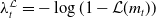 $\lambda^{\mathcal{L}}_t = -\log(1 - \mathcal{L}(m_{t}))$
and
$\lambda^{\mathcal{L}}_t = -\log(1 - \mathcal{L}(m_{t}))$
and
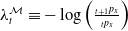 $\lambda^{\mathcal{M}}_t \equiv -\log\left(\frac{_{t+1}p_x}{_{t}p_x}\right)$
.
$\lambda^{\mathcal{M}}_t \equiv -\log\left(\frac{_{t+1}p_x}{_{t}p_x}\right)$
.
For more detailed descriptions refer to Godin et al. (Reference Godin, Hamel, Gaillardetz and Ng2023).
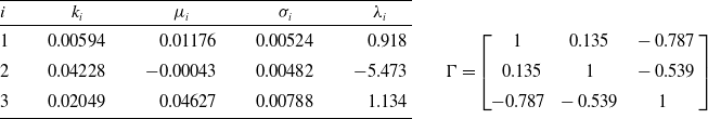
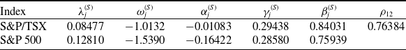

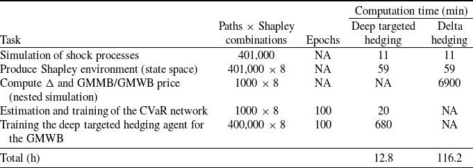
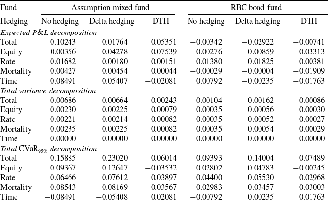
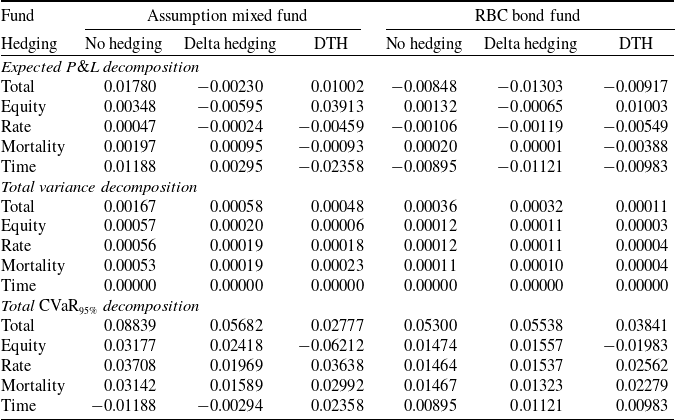
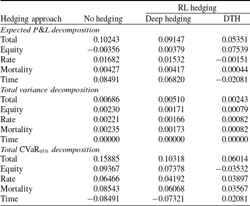
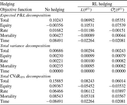


 Open access