


Introduction
Economists define the benefits of environmental quality in terms of willingness to pay (WTP). The types of benefits are determined by the purpose for which the public are willing to pay. In a typical taxonomy of total economic values, use values involve direct enjoyment or consumption of ecological services, while non-use values involve benefits derived from the existence of an environmental amenity, independent of its present or future use. Leonard et al. (Reference Leonard, Regan, Costello, Kerr, Parker, Plantinga, Salzman, Smith and Stoellinger2021) point to biases toward direct uses in past rules governing public natural resources, which highlights the importance of including both use and non-use values for efficient resource use and management.
To address this bias problem, this paper used Monte Carlo methods to examine a utility-theoretic structural approach designed to measure use and non-use values of nonmarket environmental resources. Specifically, we propose a structural estimation method that involves measures of use values and those of non-use values, by combining revealed preference and stated preferences from consequential referenda. For the revealed preference part where we derive demands from which to infer use values for environmental quality, we simulate individuals’ recreational trip behavior and use their trip costs, the latter of which were estimated based on survey data collected in 2019. Then, with simulated stated preference data, we decompose the total value into use value and non-use value that people are willing to pay to improve environmental conditions of ecosystem services. In our conceptual framework, we choose a consequential, incentive-compatible, single referendum contingent valuation method to elicit total WTP. Non-use WTP can be simultaneously and separately identified by the identification strategy we will introduce in the model section.
This approach is motivated by the policy demand and legal mandate that are required for public managed resources (Arrow et al., Reference Arrow, Cropper, Eads, Hahn, Lave, Noll, Portney, Russell, Schmalensee, Smith and Stavins1996), as well as practical concerns for research design (Smith et al., Reference Smith, Shaw, Welsh, Dixon and McDonald2022) in ecosystem services valuation. U.S. Environmental Protection Agency calls for improving the measurement of non-use benefits for proposed rules in the regulatory impact assessment and benefit-cost analysis noting that there has been a limited number of studies that U.S. Environmental Protection Agency (EPA) could draw non-use benefit estimates from for regulatory decision-making (Griffith et al. Reference Griffiths, Klemick, Massey, Moore, Newbold, Simpson, Walsh and Wheeler2012). Also, the structural approach in this paper can be applied further to estimate a complex package of ecological benefits derived from the quality changes of services that ecosystems provide. Building on the work by Day et al. (Reference Day, Bateman, Binner, Ferrini and Fezzi2019), we test the new method that combines a multi-site random utility recreation demand system with the referendum contingent valuation method. Unlike some ad hoc proposals for measuring use and non-use values, this approach can estimate individuals’ use WTP and non-use WTP portions of total value over a variety of choice alternatives within a single utility-theoretic approach.
In the model section, we define use and non-use utilities at the individual level and derive a formula for valuing use and non-use WTP. In doing so, we challenge the assumption sometimes appearing in the literature that users have only use values and non-users have only non-use values, especially since some empirical evidence shows that individuals hold both use and non-use values, regardless of their direct use of nature. Thus, we incorporate a theoretically consistent empirical framework as an alternative to ad hoc approaches to define non-use values. Then, we present Monte Carlo simulations that compare the bias and root mean squared error (RMSE) of parameter estimates for different generated data. With the data generated from these experiments, we show the consistency of the empirical method. Simulation results show that the structural method is robust but has bias under certain conditions. The upshot is that researchers pursuing this approach should be cautious with its power if they have preliminary data or priors that non-use values are small relative to use values, as our simulations show those cases are prone to some bias, whereas bias is small for a broad range of cases. We conclude the paper with a discussion of the limitations of this research and some future research topics.
Literature and background
Nonmarket valuation is a tool for economic valuation of ecosystem services based on a link between changes in the quantity or quality of the resource and the changes in the stated or observed behavior of people. The measurement of this relationship facilitates the comparison of values of nonmarket goods in monetary units. For example, contingent valuation studies have been used to assess the damages to waterbodies caused by accidents such as oil spills and inform administrative and judicial decisions (Loomis, Reference Loomis1997; Carson et al., Reference Carson, Mitchell, Hanemann, Kopp, Presser and Ruud2003; Bishop et al., Reference Bishop, Boyle, Carson, Chapman, Hanemann, Kanninen, Kopp, Krosnick, List and Meade2017; English et al., Reference English, von Haefen, Herriges, Leggett, Lupi, McConnell, Welsh, Domanski and Meade2018). Use and existence values of environmental quality changes can be measured in a hypothetical market, consistent with economic theory, and they can be used as a starting point for resource management decision of government agencies (Carson, Reference Carson2012; Kling et al., Reference Kling, Phaneuf and Zhao2012).
Of the myriad benefits that the natural environment provides, some of the values are relatively straightforward to measure through revealed market transactions (Arrow et al., Reference Arrow, Solow, Portney, Leamer, Radner and Schuman1993). For example, use values are reflected in observed behavior of individuals who actively use natural resources (recreational fishers, boaters, swimmers, hikers, and others). Individuals use environmental amenities to enhance their welfare by producing utility-yielding goods or services, or by using them as substitutes for, or complements to, market goods such as recreation trips (Freeman III et al. Reference Freeman, Herriges and Kling2014). Non-use values, however, are independent of a person’s present or future use of the resource. Broadly defined, non-users are individuals who do not use a particular site but may derive utility from its existence or for others’ use. Although alternative views exist on the definition of, classification of, and boundary between use and non-use values, Smith (Reference Smith1987) conceptualizes non-use benefits as option and existence value, the latter of which includes bequest value.
A key challenge that arises in estimating the benefits is to conceptualize non-use values and distinguish them from use values, where it is the combined use and non-use values that sum to the total economic value of resources. This is especially important for meta-analyses of values seeking to isolate the value types and for filling in gaps in literature in other areas where it becomes useful to draw upon ratios of use and non-use found in the literature (Griffiths et al., Reference Griffiths, Klemick, Massey, Moore, Newbold, Simpson, Walsh and Wheeler2012). Yet, at times a fuzzy definition of use and non-use values prevails in literature and makes it difficult to select a legitimate empirical model to determine non-use values. Some of various methods to measure non-use value are reviewed and discussed by Johnston et al. (Reference Johnston, Besedin and Wardwell2003).
A common ad hoc approach to define use and non-use is to treat use values as the value held by users and non-use values as the values held by non-users and compare total willingness to pay (WTP) for non-users with total WTP for users. For example, Croke et al. (Reference Croke, Fabian and Brenninam1987) classify survey respondents who currently use rivers as users and find that the mean willingness to pay for water quality improvements is higher among users than non-users. Whitehead et al. (Reference Whitehead, Blomquist, Hoban and Clifford1995) find the WTP of on-site users is greater than WTP of off-site users or WTP of non-users when comparing WTP of three groups (on-site users, off-site users, and non-users). Similarly, Bockstael et al. (Reference Bockstael, McConnell and Strand1989)’s contingent valuation survey results show that users are more willing to pay a tax for water quality improvements in the Chesapeake Bay, with the sample comprised of 43% users and 57% non-users. Whittington et al. (Reference Whittington, Cassidy, Amaral, McClelland, Wang and Poulos1994) also find that a typical user of Galveston Bay is more likely to support the plan for environmental quality improvement than a typical non-user. A shortcoming of this approach is that it could imply users do not have non-use values. Even the definition of “users” differs across studies. Some papers define users as visitors and non-users as non-visitors. Similarly, users may have non-use values for other recreation alternatives that they do not use. Non-users in a specific time period may hold use values for any resource at different places and times.
Another method that has been used in previous literature is to compare the WTP for different purposes: use purposes and non-use purposes. Lant and Roberts (Reference Lant and Roberts1990) let the WTP for recreational use represent use values and the WTP for intrinsic values be non-use values. They find that non-use value benefits of river quality improvement exceed the benefits for direct use. Other studies rely on the respondent’s decomposition of values into categories of use and non-use values (Roberts and Leitch Reference Roberts and Leitch1997). For example, after respondents report their total, a follow-up question would ask them to apportion the total WTP into use, option, and existence values categories (Sutherland and Walsh, Reference Sutherland and Walsh1985; Sanders et al. Reference Sanders, Walsh and Loomis1990; Kaoru, Reference Kaoru1993).
A few examples venture to estimate non-use values as the total WTP of a survey sample who were asked to assume they would not use the resource being valued. Magat et al. (Reference Magat, Huber, Viscusi and Bell2000) examine the rate of trade-off between water quality improvements in the person’s own region versus water quality improvements in a region that the respondent will not visit. They also analyze the potential values of water quality based on the probability that the respondent will visit another region. This type of research design attempts to take non-use and probabilistic use values into account.
More recently, researchers have devised more delicate survey designs and estimation strategies as methods evolve. Under a combined revealed and stated preference setting, the models estimate non-use values as total WTP of the sample of users minus estimated WTP for the direct use of the resource estimated based on revealed preference data (Eom and Larson Reference Eom and Larson2006; Whitehead et al. Reference Whitehead, Pattanayak, Van Houtven and Gelso2008; Egan, Reference Egan, Whitehead, Haab and Huang2011). Landry et al. (Reference Landry, Shonkwiler and Whitehead2020) jointly estimate models of beach recreation demand and total WTP. They find evidence of significant welfare gains from beach erosion control policies that affect beach width and coastal environmental quality with a large component for existence values.
Structural model of use and non-use values
The objective of the econometric model that is introduced here is to simultaneously estimate use and non-use values using both simulated RP and SP data (Day et al. Reference Day, Bateman, Binner, Ferrini and Fezzi2019). In this paper, the conceptual framework incorporates a single dichotomous contingent valuation question into a random utility recreation demand model, rather than repeated choice experiments as used in Day et al. (Reference Day, Bateman, Binner, Ferrini and Fezzi2019). We use a single referendum question because the approach is consequential and explore its abilities to identify the distinction of use and non-use values since a single question is less efficient than a panel of responses for each individual. The RP portion of the model uses a repeated RUM approach that captures total trips and site allocations (Freeman III et al. Reference Freeman, Herriges and Kling2014) and incorporates a full set of site-specific constants. For each individual i choosing site j with the state of environmental quality s at each choice occasion t, the joint conditional indirect utility function can be specified in an additively separable form.
 $${u_{i,t,s|j}} = v_{i,t,s|j}^{Use} + v_{i,t,s}^{NonUse} + v_{i,t,s|j}^{other} + {\varepsilon _{i,j,t,s}}$$
where the first term on the right-hand side is the conditional indirect utility from recreation activities at site j and the second term is the non-use utility gain from J different sites, independent of the recreation activity, and the third term is the utility from a composite good. All the conditional indirect utility terms besides the errors are constant over choice occasions, which will substantially simplify some terms below. The error terms are allowed to vary over choice occasions.
When individual i evaluates the option of visiting visit site j on a choice occasion t, the conditional use utility of visiting site j among J sites is a linear combination of alternative specific constant (ASC) ${\alpha _{ijt}}$
and site quality
${\alpha _{ijt}}$
and site quality ${q_{js}}$
. When individual i evaluates the option to “not go” to any site at a choice occasion at t, the conditional use utility for such opt-out choice J + 1 does not include quality and is given by
${q_{js}}$
. When individual i evaluates the option to “not go” to any site at a choice occasion at t, the conditional use utility for such opt-out choice J + 1 does not include quality and is given by ${\alpha _{i,\;J + 1,\;t}}$
.
${\alpha _{i,\;J + 1,\;t}}$
.
 $$v_{i,t,s|j}^{Use} = \left\{ {\matrix{ {{\alpha _{ijt}} + {q_{js}}\beta \;\;\;\;if\;\;j = 1,\;2,\; \ldots ,\;J} \cr \!\!\!\!\!\!\!\!\!\!\!\!\!{{\alpha _{i,\;J + 1,\;t}}\;\;\;\;\;\;\;\;\;\;\;\;\!\!\!\!\!if\;\;j = J + 1} \cr } } \right.$$
Non-use utility is characterized by the distance-weighted sum across all the non-use utility gained from sites j = 1 to J as follows:
 $$v_{i,t,s}^{NonUse} = \mathop \sum \limits_{j = 1}^J {\left( {{d_{ij}} + 1} \right)^\lambda }({a_{ijt}} + {q_{js}}b)$$
where λi is a parameter of the rate of distance decay in non-use utility. The value of λ determines how non-use utility may change with respect to distance.
Finally, the conditional utility from other consumption at choice occasion t is assumed to be linear in expenditure.
 $$v_{i,t,s|j}^{other} = \gamma \left( {{y_{i,t}} - {p_{i,j}} - {c_s}} \right)$$
where $\gamma $
is a parameter of the marginal utility of money and y
i,t
−p
i,j
−c
s
is the expenditure available for other goods. Note that p
i,j
is a travel cost of individual i for visiting site j and c
s
is the per-occasion lump-sum cost from the referendum for environmental quality change.
$\gamma $
is a parameter of the marginal utility of money and y
i,t
−p
i,j
−c
s
is the expenditure available for other goods. Note that p
i,j
is a travel cost of individual i for visiting site j and c
s
is the per-occasion lump-sum cost from the referendum for environmental quality change.
Revealed preference portion of the structural model (RP-only model)
To simulate travel cost data, we assume the trips occur in the baseline period (i.e., without environmental quality change, q j,0 ). Under the current environmental condition (s = 0), there is no fee so c i,0 = 0 for all i. In this case, the probability that individual i will choose trip alternative j on choice occasion t is given by:
 $$\begin{align*}
P{r_{i,j,t,0}} = Pr\left( {{u_{i,t,0|j}} - {u_{i,t,0|k}} > 0} \right) \\ &
\!\!\!\!\!\!\!\!\!\!\!\!\!\!\!\!\!\!\!\!\!\!\!\!\!\!\!\!\!\!\!\!\!\!\!\!\!\!\!\!\!\!\!\!\!\!\!\!\!\!\!\!\!\!\!\!\!\!\!\!\!\!\!\!\!\!\!= Pr\left[ {\left( {v_{i,0|j}^{Use} + v_{i,0}^{NonUse} + v_{i,0|j}^{other}} \right) - \left( {v_{i,0|k}^{Use} + v_{i,0}^{NonUse} + v_{i,0|k}^{other}} \right) > \;{\varepsilon _{i,k,t,0}} - {\varepsilon _{i,j,t,0}}\;} \right] \\ \end{align*}$$
$$\begin{align*}
P{r_{i,j,t,0}} = Pr\left( {{u_{i,t,0|j}} - {u_{i,t,0|k}} > 0} \right) \\ &
\!\!\!\!\!\!\!\!\!\!\!\!\!\!\!\!\!\!\!\!\!\!\!\!\!\!\!\!\!\!\!\!\!\!\!\!\!\!\!\!\!\!\!\!\!\!\!\!\!\!\!\!\!\!\!\!\!\!\!\!\!\!\!\!\!\!\!= Pr\left[ {\left( {v_{i,0|j}^{Use} + v_{i,0}^{NonUse} + v_{i,0|j}^{other}} \right) - \left( {v_{i,0|k}^{Use} + v_{i,0}^{NonUse} + v_{i,0|k}^{other}} \right) > \;{\varepsilon _{i,k,t,0}} - {\varepsilon _{i,j,t,0}}\;} \right] \\ \end{align*}$$
for all $k \ne j\; \in \left\{ {1,\; \cdots ,\;J} \right\}$
. Non-use utility
$k \ne j\; \in \left\{ {1,\; \cdots ,\;J} \right\}$
. Non-use utility $v_{i,0}^{NonUse}$
cancels out of the per choice occasion trip probabilities as it is constant for each individual i at choice occasion t, that is, an individual’s trip decision is not influenced by non-use values.
$v_{i,0}^{NonUse}$
cancels out of the per choice occasion trip probabilities as it is constant for each individual i at choice occasion t, that is, an individual’s trip decision is not influenced by non-use values.
We normalize the no trip utility to zero because only the difference between the trip utilities of choice alternatives matters in discrete choice models.
 $$P{r_{i,j,t,0}} = Pr \left( {{u_{i,t,0|j}} - {u_{i,t,0|k}} \gt 0} \right) = Pr \left[ {v_{i,0|j}^{RP} - v_{i,0|k}^{RP} \gt \;{\varepsilon _{i,k,t,0}} - {\varepsilon _{i,j,t,0}}\;} \right] = P{r_{i,j,0}}$$
Adding SP data with non-use values to the structural model (Joint RP-SP model)
Next, we add simulated SP data with both use and non-use values in the model. The annual joint utility that individual i receives from choosing from a state of the world s (s = 0, 1) is
 $${u_{i, \cdot ,s}} = {\tilde v_{i, \cdot ,s}} + {\tilde \varepsilon _{i, \cdot ,s}} = \sum _{t = 1}^T{\tilde v_{i,s}} + \sum _{t = 1}^T{\tilde \varepsilon _{i,s}} = T{\tilde v_{i,s}} + \sum _{t = 1}^T{\tilde \varepsilon _{i,s}}$$
where the deterministic term of the annual utility is the expected maximum utility per-choice occasion times the number of choice occasions.
The expected maximum joint utility of each individual i receiving use value from taking trips and non-use under a state of the world s can be written as
 $${\tilde v_{i,}} = \mathbb{E} \left[ {\mathop {\max }\limits_{j \in \left\{ {1,2, \cdots ,J + 1} \right\}} \left( {v_{i,s|j}^{Use} + v_{i,s|j}^{other} + \varepsilon _{i,j,t,s}^{Use}} \right)} \right] + {{v_{i,0}^{NonUse}} \over {{\sigma ^{SP}}}}$$
For specification of the trip-taking random utility model, the errors $\varepsilon _{i,j,t,s}^{Use}$
are assumed to follow a Type 1 extreme value error term with a scale factor of
$\varepsilon _{i,j,t,s}^{Use}$
are assumed to follow a Type 1 extreme value error term with a scale factor of ${\sigma ^{RP}}$
, which is not separately identified in conditional logits and is normalized
${\sigma ^{RP}}$
, which is not separately identified in conditional logits and is normalized ${\sigma ^{RP}}$
to be 1. While
${\sigma ^{RP}}$
to be 1. While $\varepsilon _{i,j,t,s}^{Use}$
has a t subscript, the expectation does not depend on t since the
$\varepsilon _{i,j,t,s}^{Use}$
has a t subscript, the expectation does not depend on t since the $\varepsilon _{i,j,t,s}^{Use}$
’s are identically distributed over time. Following assumptions made in Day et al. (Reference Day, Bateman, Binner, Ferrini and Fezzi2019) paper, the joint use and non-use utility function takes a log sum form, plus a constant
$\varepsilon _{i,j,t,s}^{Use}$
’s are identically distributed over time. Following assumptions made in Day et al. (Reference Day, Bateman, Binner, Ferrini and Fezzi2019) paper, the joint use and non-use utility function takes a log sum form, plus a constant $\kappa $
.
$\kappa $
.
 $${\tilde v_{i,s}} = {1 \over {{\sigma ^{SP}}}}\ln \left[ {\sum\limits_{j = 1}^{J + 1} {\exp } \left( {v_{i,s|j}^{Use} + v_{i,s|j}^{other}} \right)} \right] + \kappa + {{v_{i,0}^{NonUse}} \over {{\sigma ^{SP}}}}\;$$
where $\kappa $
is a constant of integration for the expected value of a maximum of extreme values (Johnson and Kotz, Reference Johnson and Kotz1969). The scale parameter
$\kappa $
is a constant of integration for the expected value of a maximum of extreme values (Johnson and Kotz, Reference Johnson and Kotz1969). The scale parameter ${\sigma ^{SP}}$
characterizes the relative variation in the SP data compared to the RP data. From empirical studies in the literature, we expect SP data to show greater variability than RP data (i.e.,
${\sigma ^{SP}}$
characterizes the relative variation in the SP data compared to the RP data. From empirical studies in the literature, we expect SP data to show greater variability than RP data (i.e., ${\sigma ^{SP}}$
> 1).
${\sigma ^{SP}}$
> 1).
Then, we can derive the choice probability that individuals would choose the proposed quality change scenario (s = 1) in terms of the difference between joint utilities before and after the change.
 $$Pr ({u_{i, \cdot ,1}} \gt {u_{i, \cdot ,0}}) = Pr ({\tilde v_{i, \cdot ,1}} - {\tilde v_{i, \cdot ,0}} \gt {\tilde \varepsilon _{i, \cdot }})$$
To derive the choice probability of individuals choosing the quality change scenario (s = 1) compared to the baseline environmental condition (s = 0), kappa is the same in ${\tilde v_{i, \cdot ,1}}$
and
${\tilde v_{i, \cdot ,1}}$
and ${\tilde v_{i, \cdot ,0}}$
and cancels out. This choice probability can be rewritten as the cumulative distribution function for the difference in errors
${\tilde v_{i, \cdot ,0}}$
and cancels out. This choice probability can be rewritten as the cumulative distribution function for the difference in errors ${\widetilde \varepsilon _{i, \cdot }} = {\tilde \varepsilon _{i,t,0}} - {\tilde \varepsilon _{i,t,1}}$
. Assuming that
${\widetilde \varepsilon _{i, \cdot }} = {\tilde \varepsilon _{i,t,0}} - {\tilde \varepsilon _{i,t,1}}$
. Assuming that ${\widetilde \varepsilon _{i, \cdot }}$
follows a logistic distribution of (0, 1), the difference in error term
${\widetilde \varepsilon _{i, \cdot }}$
follows a logistic distribution of (0, 1), the difference in error term ${\widetilde \varepsilon _{i, \cdot }}$
approximately follows a t-distribution
${\widetilde \varepsilon _{i, \cdot }}$
approximately follows a t-distribution ${t_{5T + 4}}\left( {0,\tau } \right)$
where
${t_{5T + 4}}\left( {0,\tau } \right)$
where $\tau = \pi {\left( {{{15T + 12} \over {5{T^2} + 2T}}} \right)^{ - {1 \over 2}}}$
(George and Mudholkar, Reference George and Mudholkar1983; Day et al., Reference Day, Bateman, Binner, Ferrini and Fezzi2019).
$\tau = \pi {\left( {{{15T + 12} \over {5{T^2} + 2T}}} \right)^{ - {1 \over 2}}}$
(George and Mudholkar, Reference George and Mudholkar1983; Day et al., Reference Day, Bateman, Binner, Ferrini and Fezzi2019).
The resulting likelihood function characterizes individual i’s revealed preference for recreational sites along with their stated preference choices when choosing the sites to visit and the vote to make in the referendum. Specifically,
 $${L_i}\left( {{{\boldsymbol\theta} _i}} \right) = \prod\limits_t {} \prod\limits_j {\matrix{ {P{r_{i,j,t}}{{\left( {{\boldsymbol\theta}_{}^{\boldsymbol Use},\;\gamma } \right)}^{{Y_{i,j,t}}}}} \cr } } \prod\limits_s P {r_{i,s}}{\left( {{\boldsymbol\theta}_{}^{\boldsymbol Use},{\boldsymbol\theta} _{}^{\boldsymbol NonUse},\;\gamma } \right)^{{Y_{i,s}}}}$$
where ${\boldsymbol\theta} = \left[ {{\boldsymbol\theta} _{}^{\boldsymbol Use},\;{\boldsymbol\theta} _{}^{\boldsymbol NonUse},\;\lambda } \right]$
are parameters of interest in the structural model of use and non-use values.
${\boldsymbol\theta} = \left[ {{\boldsymbol\theta} _{}^{\boldsymbol Use},\;{\boldsymbol\theta} _{}^{\boldsymbol NonUse},\;\lambda } \right]$
are parameters of interest in the structural model of use and non-use values. ${\boldsymbol\theta} _{}^{\boldsymbol Use} = \left[ {{\alpha _1},{\rm{\;}} \ldots ,{\rm{\;}}{\alpha _J},{\rm{\;}}\beta } \right]$
denote the parameters of the use utility, and
${\boldsymbol\theta} _{}^{\boldsymbol Use} = \left[ {{\alpha _1},{\rm{\;}} \ldots ,{\rm{\;}}{\alpha _J},{\rm{\;}}\beta } \right]$
denote the parameters of the use utility, and ${\boldsymbol\theta} _{}^{\boldsymbol NonUse} = \left[ {b,{\rm{\;}}\lambda } \right]$
denote the identifiable parameters of the non-use utility. The maximum log-likelihood estimation program solves
${\boldsymbol\theta} _{}^{\boldsymbol NonUse} = \left[ {b,{\rm{\;}}\lambda } \right]$
denote the identifiable parameters of the non-use utility. The maximum log-likelihood estimation program solves
 $${L_{SP}} = log({L_i}({{\boldsymbol\theta} _i})) = Y_i^{SP}\,{\rm{ln}}[{F_{\tilde \varepsilon }}({\tilde v_{i, \cdot ,1}} - {\tilde v_{i, \cdot ,0}})] + (1 - Y_i^{SP}){\rm{ln}}[1 - {F_{\tilde \varepsilon }}({\tilde v_{i, \cdot ,1}} - {\tilde v_{i, \cdot ,0}})]$$
Once we have estimated parameters, we can compute welfare measures. Since researchers do not observe true utilities, welfare changes are taken using expectations of outcomes from the random utilities with and without a change (Freeman III et al. Reference Freeman, Herriges and Kling2014). The per-choice occasion willingness to pay for the use benefits from the policy change takes the form
 $$WT{P^{Use}} = {1 \over \gamma }ln\left[ {\;{{\sum\nolimits_{j = 1}^{J + 1} {{\rm{exp}}} \left( {{{\tilde \alpha }_j} + {\Delta _{i,j,1}}\beta - \gamma {p_{i,j}}} \right)} \over {\sum\nolimits_{j = 1}^{J + 1} {{\rm{exp}}} \left( {{{\tilde \alpha }_j} - \gamma {p_{i,j}}} \right)}}\;} \right]$$
where the marginal use utility divided by the marginal utility of money ( $\gamma $
) and Δ represents a change in quality. Likewise, the per-choice occasion willingness to pay for the non-use benefits from the environmental quality change is calculated by the change in non-use utility. The division by
$\gamma $
) and Δ represents a change in quality. Likewise, the per-choice occasion willingness to pay for the non-use benefits from the environmental quality change is calculated by the change in non-use utility. The division by $\gamma $
translates utility into dollars and yields
$\gamma $
translates utility into dollars and yields
 $$WT{P^{Nonuse}} = {1 \over \gamma }\ln \left[ {\;\sum\limits_{j = 1}^J {{{\left( {{d_{i,j}} + 1} \right)}^\lambda }} {\Delta _{i,j,1}}b\;} \right]$$
Monte Carlo simulation
This section evaluates the performance of the structural estimation program to measure use and non-use values for improved environmental quality. We follow the modeling procedures to generate the data and set up the maximum likelihood function. We first estimate the structural model assuming that the non-use component of overall utility is zero. We then incorporate a non-use component into overall utility. The primary reason for the Monte Carlo simulation is that given the single SP observation per person, the full set of recreation site-specific fixed effects, and the highly nonlinear nature of the model and the corresponding log-likelihood function, the Monte Carlo exercise provides potentially useful insights into difficulties one might encounter in estimating the structural model, including potential problems with identification or local optima. This will be useful for future valuation efforts in considering whether to apply the method.
Monte Carlo simulation set-up
The key idea of the Monte Carlo (MC) exercise is to generate simulated data to estimate two models in sequence: (1) a discrete choice random utility model of recreation demand based on the revealed preference portion of the structural model (i.e., RP model) for starting values and (2) a joint revealed and stated preference model for use and non-use values (i.e., joint RP-SP model). Portions of the simulated data are drawn to represent the types of preferences and range of some of some existing studies. The data are also drawn using information from the survey used in Lupi et al. (Reference Lupi, Herriges, Kim and Stevenson2023) and are designed to mimic some characteristics of a general population survey which will be used in a future empirical application (the survey was recently used in Sandstrom-Mistry et al., Reference Sandstrom-Mistry, Lupi, Kim and Herriges2023).
After drawing simulated data, the algorithm uses GAUSS’s maximum likelihood routine to estimate a repeated random utility maximization (RUM) model using revealed reference data alone. This program estimates the ASCs, which are site-specific fixed effects for the site attributes, and the parameter of marginal utility of income given by the negative of the parameter on travel costs to each site. Then, those parameters are used as initial values in the joint estimation of the structural model of use and non-use values. Specifically, the program uses the joint log-likelihood function and both simulated RP and SP data to estimate the marginal use utility of environmental quality improvement (β), the marginal non-use utility of environmental quality improvement (b), the distance decay parameter ( $\lambda $
), and the scaling factor for the variation of error terms (σ), as well as updating the ASCs (α’s) and the marginal utility of income parameters (γ).
$\lambda $
), and the scaling factor for the variation of error terms (σ), as well as updating the ASCs (α’s) and the marginal utility of income parameters (γ).
In conducting the Monte Carlo exercise, we consider a variety of parameter configurations defined in terms of alternative levels for β, b, and σ. For each of these parameter combinations, the MC exercise proceeds in seven steps reported in Table 1. In addition, the MC exercise produces mean and median estimates of the parameters of interest and their 90% confidence interval. It also calculates four key variables: (1) the implied stay-at-home probabilities under the proposed parameter configuration, (2) the implied average probabilities of responding yes to the SP scenario for environmental quality change, (3) willingness to pay (WTP) for the use benefits from the scenario, and (4) WTP for the non-use benefits from the scenario. For each of these, minimum, mean, and maximum values are reported.
Monte Carlo steps for each parameter configuration {β, b, and σ}

Table 2 presents the design for some of the levels used in the Monte Carlo analyses. The design is intended to cover a range for relative use and non-use values similar in spirit to the mixed results found in the literature.
Monte Carlo design

Additional details and rationale for the Monte Carlo design follow:
Number of observations (N): Since the sample size of some valuation studies focusing on environmental resources is around 300 for smaller studies (Caudill et al., Reference Caudill, Groothuis and Whitehead2011), about 2,000 for many studies (Kotchen et al. Reference Kotchen, Moore, Lupi and Rutherford2006; Knoche and Lupi Reference Knoche and Lupi2007; Melstrom et al. Reference Melstrom, Lupi, Esselman and Stevenson2015), with only a few national-level studies gather samples with more than 10,000 observations (English et al., Reference English, von Haefen, Herriges, Leggett, Lupi, McConnell, Welsh, Domanski and Meade2018; Day, Reference Day2020), we use 2,000 to represent common empirical studies. To ensure that estimators of parameters converge in probability to the true value of each parameter, simulations were also run with larger sample size (N = 5,000), in which case the magnitude of bias diminished. The simulation results implied the structural method generally preserves the consistency of estimator.
Number of recreational sites (J): we set the number of sites to be 38. We also tested the estimation routine and found similar results in a setting with a small number of sites, as well as a larger number of sites.
Number of choice occasions (T): In recreation demand literature, a sufficiently large number, and sometimes the maximum number of trips taken during the study period, is typically chosen for the number of choice occasions to avoid trimming the trip data. Here we choose T = 30 to match a typical study for summer trips (Lupi et al., Reference Lupi, von Haefen and Cheng2022).
The travel costs ( p ij ): Travel costs were randomly drawn from an existing survey sample trip data set that contain residence locations, site travel distances, site travel times, incomes of Michigan residents (Lupi et al., Reference Lupi, Herriges, Kim and Stevenson2023). The cost of not taking a trip is zero for everyone. In the simulation, travel costs are drawn independent of unobserved site characteristics.
The marginal utility of income parameter (γ): In our MC exercise, we set γ to be −0.40. Initial values for this parameter value are estimated from a logit recreation demand model, in which the travel cost parameter is estimated using revealed preference data from other survey data (Kim et al., Reference Kim, Lupi and Herriges2023).
Alternative Specific Constants (ASCs): The ASCs are set to ensure that the average probability that an individual will stay at home on a given choice occasion (i.e., Probi,J+1) is approximately 0.17, which amounts to about 5 trips per person per year based on other existing survey data (Lupi et al., Reference Lupi, Herriges, Kim and Stevenson2023). These site-fixed effects are assumed to be the same for all individuals. We use a full set of fixed effects (ASCs) for each of the J sites in the Monte Carlo exercise.
Proposed stated preference scenarios: The simulation scenarios vary parameter configurations along two dimensions: the change in environmental quality improvement (Δq), and the contingent valuation cost levels (C). The change in environmental quality at each site is drawn randomly in the range of 0 to 10. The value for the change in environmental quality is heterogeneous across individuals. That mimics the experimental design in recent contingent valuation setting, where individuals face different scenarios of one proposed environmental quality improvement and corresponding cost (Sandstrom-Mistry et al., Reference Sandstrom-Mistry, Lupi, Kim and Herriges2023). In Monte Carlo simulation exercise, the contingent valuation cost level is also drawn randomly across individuals. The range of the contingent valuation scenario cost is [0, 50] per-choice occasion. It means that individuals agree to pay the per-choice occasion policy cost if individuals decide to vote for a proposed environmental quality change.
Scaling Parameter ( σ ): Estimation of the joint RP-SP model provides estimates of the common parameters along with any RP-specific and SP-specific model parameters. A “scale” parameter represents the relative scale of the coefficients of the RP-only model and joint RP-SP model since the variances of the random components of the RP and SP utility functions are likely to differ (Ben-Akiva et al., Reference Ben-Akiva, Bradley, Morikawa, Benjamin, Novak, Oppewal and Rao1994). The scale parameter was set at σ = [1, 2, 3] with the one implying equal variance in the RP and SP data and the larger levels mirroring or exceeding levels found in other studies, such as Day et al. (Reference Day, Bateman, Binner, Ferrini and Fezzi2019).
Distance ( d ij ): Distance is the straight-line distance from an individual’s home to trip destination j. In the simulation, we set this straight-line distance to be a random proportion of travel cost based on an examination of existing data. We set the non-use distance decay parameter λ to a negative value (i.e., λ = −1) as is often found in the literature. It means that sites closer to an individual’s home have more non-use value than more distant sites. That is, the non-use utility from improved environmental quality benefits at site j diminishes as individuals live far from the site.
Monte Carlo simulation results
The RP-only model estimation produces the estimates of common parameters: the parameter estimates of ASCs (each α
j
) and the marginal utility of income ( $\gamma $
). The joint RP-SP model adds four additional parameters to those identified in the RP-only model: marginal use utility of environmental quality (β), marginal non-use utility of environmental quality (b), a non-use distance decay (λ), and a scaling factor (
$\gamma $
). The joint RP-SP model adds four additional parameters to those identified in the RP-only model: marginal use utility of environmental quality (β), marginal non-use utility of environmental quality (b), a non-use distance decay (λ), and a scaling factor ( $\sigma $
). We summarize the result of the Monte Carlo simulation experiments and compare four tables for the generalized structural RP-SP model in this section.
$\sigma $
). We summarize the result of the Monte Carlo simulation experiments and compare four tables for the generalized structural RP-SP model in this section.
In this section, we primarily focus our attention on the two environmental quality parameters (β and b) to check the model performance when estimating the key parameters of interest (Table 3). Then, in the second table (Table 4), we investigate the extent of estimation errors on the travel cost parameter ( $\gamma $
) and the ASCs (each α
j
) as they are also key determinants of welfare measures. Both tables include the root mean square errors (RMSEs) and percentage RMSEs results for two versions of joint RP-SP models. In the first sub-column, denoted as “λ fixed,” the distance decay parameter λ is fixed as a constant at the true level and is not estimated. The second sub-column, denoted as “λ est.,” estimates the distance decay parameter.
$\gamma $
) and the ASCs (each α
j
) as they are also key determinants of welfare measures. Both tables include the root mean square errors (RMSEs) and percentage RMSEs results for two versions of joint RP-SP models. In the first sub-column, denoted as “λ fixed,” the distance decay parameter λ is fixed as a constant at the true level and is not estimated. The second sub-column, denoted as “λ est.,” estimates the distance decay parameter.
Monte Carlo simulation results – Key parameter estimates of interest

Note: All runs with sample set at N = 2,000 using R = 1,000 replications.
Monte Carlo simulation results – Site fixed effects and cost coefficient
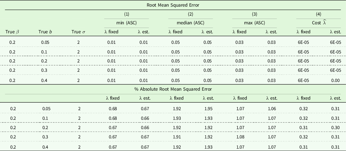
Note: All runs with sample set at N = 2,000 using R = 1,000 replications. True λ is −1 for all cases.
Table 3 presents true values of key parameters of interest ( ${\rm{\beta }}$
,
${\rm{\beta }}$
, $b$
,
$b$
, $\sigma $
, λ), root mean squared error (RMSE), and the percentage root mean squared error (%RMSE) of estimates of each parameter. The first three columns are true values. The latter columns compare RMSE and %RMSE of two models. Compared to the RMSE of the use quality parameter estimates, the RMSE of the non-use quality parameter estimates is slightly larger in both “λ fixed” and “λ est.” models. The same is true for %RMSE. It implies that the use quality parameter is more precisely estimated than the non-use quality parameter or the scaling factor parameter. Both RMSE and %RMSE values are larger when λ is estimated than when λ is known. The magnitude of RMSE and %RMSE of the distance decay parameter diminish as the true value of the non-use quality parameter estimates increases. When the marginal utility gain from the non-use portion is particularly large, the distance decay effect seems to be more easily detected.
$\sigma $
, λ), root mean squared error (RMSE), and the percentage root mean squared error (%RMSE) of estimates of each parameter. The first three columns are true values. The latter columns compare RMSE and %RMSE of two models. Compared to the RMSE of the use quality parameter estimates, the RMSE of the non-use quality parameter estimates is slightly larger in both “λ fixed” and “λ est.” models. The same is true for %RMSE. It implies that the use quality parameter is more precisely estimated than the non-use quality parameter or the scaling factor parameter. Both RMSE and %RMSE values are larger when λ is estimated than when λ is known. The magnitude of RMSE and %RMSE of the distance decay parameter diminish as the true value of the non-use quality parameter estimates increases. When the marginal utility gain from the non-use portion is particularly large, the distance decay effect seems to be more easily detected.
There are some notable findings we can draw from the simulations. First, the joint RP-SP approach with constant distance decay parameter (λ fixed) successfully recovers the underlying use and non-use quality parameters, with a RMSE of 0.03. However, converting RMSEs into the % RMSE terms, we find the %RMSE of use quality parameter increases as the true value of the non-use quality parameter increases. Conversely, the %RMSE of non-use quality parameter decreases as the true value of the non-use quality parameter increases.
Second, the joint RP-SP model that estimates a distance decay parameter (λ est.) also performs quite well on estimating the use quality parameter, with a RMSE less than 0.02 for ( $\hat \beta $
). However, it does not do as well on estimating non-use quality parameter (
$\hat \beta $
). However, it does not do as well on estimating non-use quality parameter ( $\hat b$
) or scaling factor (
$\hat b$
) or scaling factor ( $\hat \sigma $
), particularly when the true value of the non-use quality parameter is very small. Adding additional dimension into the model by estimating the distance decay parameter results in 10 times larger %RMSE.
$\hat \sigma $
), particularly when the true value of the non-use quality parameter is very small. Adding additional dimension into the model by estimating the distance decay parameter results in 10 times larger %RMSE.
Table 4 provides the RMSE and the %RMSE of estimates of three ASCs and the marginal utility of cost parameter γ. As in Table 3, assumed true values of two key parameters of interest ( $\beta $
,
$\beta $
, $\sigma $
) remain unchanged while we vary the marginal non-use utility of quality changes (
$\sigma $
) remain unchanged while we vary the marginal non-use utility of quality changes ( $b$
). Of 38 ASCs, column (1) reports the RMSE and %RMSE values of the minimum ASC; column (2) reports them for the median ASC; and column (3) reports them for the maximum ASC. Starting with the results for the travel cost coefficient in the column (4), both joint RP-SP models (with λ fixed and λ est.) do an excellent job recovering the underlying price coefficient, with the RMSE less than 0.001, perhaps to the variation across people and sites that exists for travel costs. The models also do a good job in recovering the underlying ASCs, regardless of the magnitude of the ASCs.
$b$
). Of 38 ASCs, column (1) reports the RMSE and %RMSE values of the minimum ASC; column (2) reports them for the median ASC; and column (3) reports them for the maximum ASC. Starting with the results for the travel cost coefficient in the column (4), both joint RP-SP models (with λ fixed and λ est.) do an excellent job recovering the underlying price coefficient, with the RMSE less than 0.001, perhaps to the variation across people and sites that exists for travel costs. The models also do a good job in recovering the underlying ASCs, regardless of the magnitude of the ASCs.
The RMSE remains very low in all cases and the % absolute RMSE also very small regardless of the true values of parameters of the interest. Although we report only the results of three ASCs, no obvious relationship has been found between the magnitude of true ASCs and their RMSEs/%RMSEs for each of the ASCs. Across different parameter spaces, the RMSE and %RMSE of ASCs and the cost parameter remain at similar levels. It implies that ASCs and the cost parameter estimation are quite stable across various true values of the non-use quality parameter. While the overall use and non-use model is not mean fitting for site choices, that property would hold for the use value portion of the use value only portion of the joint utility, so it is perhaps unsurprising that the approach replicates the ASCs well.
Table 5 reports the difference between the medians of true WTP and WTP estimates. We find that the magnitude of the WTP estimates is similar to that of true WTP when we evaluate at the median of the estimated parameters. The distribution of WTP estimates also remains close to the true distribution of WTP.
Difference between median WTP estimates and median true WTP ($’s)

Note: N = 2000, R = 1000. Note that the difference in true WTP and estimated WTP was calculated based on the median of true WTP and the median of parameter estimates in the joint RP-SP models which mutes the underlying variation that would be seen if I calculate WTP for each of the 2000 people for the 1000 runs (authors can provide this if desired).
Conclusion
Ecosystem services generally provide both use and non-use economic values. We began by noting an existing discrepancy among the valuation methods to measure non-use values, especially for environmental resources. We highlighted a structural estimation framework that allows decomposition of use and non-use values. WTP estimates from this model provide specific information to policy makers and federal agencies, by linking the change of ecosystem services to individual WTPs for use and non-use. Information on ratios of use and non-use values for different ecosystem services is often critical when time pressures or budgets restrict the available information for decision-making in the extant literature.
We use data-generated experiments to demonstrate that the proposed structural model generally, but not always, provides consistent results in estimating true values of parameters of interest and recovering true WTPs, which can be applied to a wide range of valuation studies. This Monte Carlo study indicates that the structural model estimates of use and non-use values have the lowest bias when the marginal utility of use and non-use quality are at a comparable level, and the performance in situations where the relative use and non-use value are more divergent is poor for some parameters of interest. We recognize that the structural model can be sensitive to research design (e.g., the variation in environmental quality within RP or SP data), while the conceptual framework can be applied to any setting involving pooling different types of choice data (i.e., portfolio choices and general purchase decisions) or requiring testing of estimator properties with complex empirical data. Since having rich revealed preference data and appropriate stated preference data enables and helps to quantify use and non-use WTP at the same time, the results show attention should be paid to these in the data collection and survey design of studies implementing the approach.
Future work should focus on addressing two concerns: (1) choice of the type of stated preference data and (2) revealed preference model specification. As many previous works find a trade-off between incentive compatibility and the number of choices, some research designs will work well with this type of model, but others do not. In cases where there is limited variation in stated choices (i.e., in a consequential single referendum choice per person), the results may provide biased value estimates. Second, future research would assist with understanding whether and to what extent use and non-use values would be impacted by other revealed preference model specifications (i.e., single site demand model, Kuhn-Tucker model, or count models).
Supplementary material
To view supplementary material for this article, please visit https://doi.org/10.1017/age.2023.26
Data availability statement
The data that support the findings of this study are available on request from the corresponding author.
Acknowledgments
Special thanks are due to Joseph A. Herriges for his help with all aspects of this work and to R. Jan Stevenson for his efforts toward the project.
Funding statement
This paper was developed under Assistance Agreement No. R836168 awarded by the U.S. Environmental Protection Agency to Lupi, Herriges, and Stevenson. It has not been formally reviewed by EPA. The views expressed in this document are solely those of the authors and do not necessarily reflect those of the Agency. EPA does not endorse any products or commercial services mentioned in this publication. Lupi received support from USDA NIFA, Michigan Department of Natural Resources and Michigan State University’s AgBioResearch.
Competing interests
The authors have no conflicts of interest to declare.


 Open access