





Nomenclature
- b
-
wingspan, m
- F
-
fuel capacity, L
- L f
-
aircraft length, m
- MTOW
-
maximum take-off weight, kg
(Note: In this paper, weight is expressed in kilograms as a mass-equivalent for consistency with industry practice)
- P
-
engine power, kW
- PAX
-
number of passengers (including crew)
- R
-
range, km
- S
-
wing area, m2
- V c
-
cruise speed, km/h
- ${W_{to}}$
-
actual maximum take-off weight, kg
-
${W_{to.est\;\left[ {cat.\;\;x} \right]}}$
-
maximum take-off weight estimate, where suffix x denotes aircraft category type (A, B, or C), kg


1.0 Introduction
Many parameters impact the aircraft design. Among these parameters, maximum take-off weight (MTOW) is critically important. MTOW must be kept under control throughout all design phases. More specifically, it is an essential parameter in evaluating aircraft performance, whereas aircraft cost, a crucial parameter for airliners (customers), is largely based on aircraft weight. Other parameters, such as fuel, thrust and lift, also depend on MTOW [Reference Obert1]. Furthermore, modelling MTOW is important in more fundamental air traffic management (ATM) studies [Reference Sun, Ellerbroek and Hoekstra2]. Aircraft manufacturers and designers endeavour to apply new materials and technologies to lighten the aircraft as much as possible, without compromising the performance or the structural strength. The top-level aircraft requirements allow designers to settle on key design variables, but accurately predicting MTOW at early design stages remains challenging. When more detailed design drawings are sketched, each component can be evaluated accurately, and the MTOW is easily determined by adding up all the components. Consequently, different methods and strategies are concurrently applied across each design phase. For instance, the first design phase (conceptual) , has methods of significant uncertainty and simplicity. In contrast, the second design phase (preliminary) uses more accurate and complex methods, as the aircraft weight is divided into components and sub-components [Reference Sun, Blom, Ellerbroek and Hoekstra3]. In other words, as more information becomes available during the design phases, the error accuracy is reduced to 5–10% in the preliminary phase, while it is typically 10–15% in the conceptual phase. For light aircraft, a 5% error means less than a 100 kg difference between the actual and estimated MTOW, which limits changes and component and instrument choices in later phases. This challenge motivates researchers/designers to develop more accurate MTOW estimation models at an early stage using crucial design parameters.
Traditional techniques have shown success in aircraft design, but their limitations are well apparent when accounting for current aircraft design complexity and the evolving bases of operation. Therefore, researchers and designers are motivated to adapt traditional techniques or develop novel approaches, such as statistical modelling and machine learning (ML), to enhance the accuracy and effectiveness of MTOW estimation. Generally, ML is required to gather relevant data (various aircraft samples with similar characteristics), perform pre-processing and conduct training and validation. The model’s success is based on the value and representativeness of the training data. Due to a lack of relevant data, ML has not yet been successfully applied to the early stages of aircraft design.
On the other hand, the application of statistical approaches to MTOW estimation has been a subject of interest in the field of aircraft design and performance analysis. The MTOW is a critical parameter influencing various aspects of aircraft operation, and employing statistical models facilitates a data-driven understanding of the relationships between design parameters and the final take-off weight. Recent trends in the literature point towards the use of Bayesian methods [Reference Sun, Ellerbroek and Hoekstra4] and Gaussian process regression [Reference Chati and Balakrishnan5] for MTOW estimation. Despite the successes, the challenges that persist in refining statistical models for MTOW estimation, and the limitations of traditional regression models, emphasise the need to incorporate more advanced statistical techniques to address non-linearity and multicollinearity among design parameters.
In response to the limitations of existing techniques and the evolving landscape of aircraft design, this research introduces a novel statistical approach for weight estimation in light aircraft. Drawing on gaps identified in the literature, this research seeks to bridge the divide by leveraging multilinear regression and p-value analysis. It aims to address the shortcomings of previous methods while providing a more robust framework for capturing the complexities inherent in light aircraft design. By building on knowledge gleaned from previous studies and integrating state-of-the-art statistical techniques, this research aims to contribute to the evolving field of aircraft weight estimation.
2.0 Theoretical background
Traditional approaches for estimating the MTOW of aircraft have long served as foundational approaches in the aircraft industry. These methodologies typically rely on established aircraft design principles, engineering calculations and historical data analysis. As a result, the traditional methods of estimating MTOW encompass well-established practices, including adherence to standard guidelines, utilisation of empirical formulas, reference to payload-range diagrams and consultation of performance charts [Reference Basgall, Liu, Cassady and Anemaat6]. The breakdown weight-estimate technique, which decomposes the MTOW into components such as empty weight, fuel weight and payload weight, is widely used in aircraft design [Reference Lee and Chatterji7] and is extensively explained in several textbooks [Reference Raymer8, Reference Kundu, Price and Riordan9]. Each component in this technique is determined using analytical methods, historical data and design configurations, employing a wide range of assigned/estimated design variables. More specifically, this technique plays a critical role in ensuring that the aircraft’s structure, systems and propulsion are properly balanced to meet the predetermined weight requirements.
On the other hand, the parametric estimation approach implies developing and applying formulae that illustrate the relationship between the target (dependent) parameter (e.g. weight, cost, volume, power, etc.) and several source (independent) parameters that should be carried out, continued and aged. In other words, parametric estimation depends on simulated models, which are statistical-based equations. The mathematical approach to estimating weight is known as parametric weight estimation (PME), like the parametric cost estimation presented in Ref. [Reference Dean10]. It replaces the target parameter with weight instead of cost. This paper employed non-weight parameters (design variables) to estimate the MTOW of light aircraft. Multiple linear regression, combined with p-value analysis, is used to develop a weight estimation model with the fewest design variables for light aircraft with an MTOW of less than 5,700 kg.
2.1 Multiple linear regression (MLR)
The linear relationship between a particular independent variable and its response is known as ordinary (simple) linear regression (OLR (SLR)), while for multiple independent variables and a single response, it is known as multiple linear regression (MLR) [Reference Chatterjee and Simonoff11]. For instance, if there are n independent variables, then an MLR model obtains the formula:
 \begin{align}\;y = {\beta _0} + {\beta _1}{x_1} + {\beta _2}{x_2} + \ldots + {\beta _n}{x_n} + \varepsilon \end{align}
where the j
th
independent variable is x
j
; the response variable is y; the error term is $\varepsilon$
; and
$\varepsilon$
; and $\beta_{j}$
is the mean impact on y of a one-unit increment in x
j
, keeping all other independent variables unchanging. The values of
$\beta_{j}$
is the mean impact on y of a one-unit increment in x
j
, keeping all other independent variables unchanging. The values of $\beta_{0},\ldots,\beta_{n}$
are obtained using the least squares method to reduce the sum of squared residuals (SSR). This method relies on matrix algebra to find the
$\beta_{0},\ldots,\beta_{n}$
are obtained using the least squares method to reduce the sum of squared residuals (SSR). This method relies on matrix algebra to find the $\beta$
coefficient estimates:
$\beta$
coefficient estimates:
 \begin{align}SSR = \sum {\left( {{y_j} - {{\hat y}_j}} \right)^2}\end{align}
where the actual response value for the j
th
sample and the predicted response value based on the MLR model is ${\hat y_j}$
. Note that evaluating these coefficient estimates requires matrix algebra. Luckily, statistical software such as Excel and SPSS can calculate these coefficients. In this work, MS Excel was used.
${\hat y_j}$
. Note that evaluating these coefficient estimates requires matrix algebra. Luckily, statistical software such as Excel and SPSS can calculate these coefficients. In this work, MS Excel was used.
2.1.1 Interpreting the MLR output
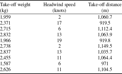
Let us have a simple example to understand the MLR output [Reference Bazdaric, Sverko, Salaric, Martinovic and Lucijanic12]. Suppose we have a response variable, take-off distance (m), and two independent variables: aircraft take-off weight (kg) and headwind speed (knots). Table 1 lists the values of the two independent variables and their relevant responses for ten aircraft samples.
The ten values of the two independent variables and the response

The MLR output might look like Fig. 1, generated in Excel.
A sample of MLR output in Excel.

From Fig. 1, the mathematical MLR model can be formulated as:
 \begin{align}takeoff\,distance = 849.1245 + 0.1198 \times takeoff\,weight - 9.7545 \times headwind\end{align}
The coefficients can be interpreted as:
-
(a) Increasing the independent variable take-off weight by one kilogram is coupled with a 0.1198 m increase in take-off distance, assuming the headwind speed is kept unchanged.
-
(b) Increasing the headwind speed by one knot is coupled with a 9.7545 m decrease in take-off distance, assuming the take-off is unchanged.
-
(c) The model can predict the take-off distance of an aircraft if the aircraft’s take-off weight and headwind speed are known. For instance, if an aircraft weighing 2,200 kg with a 10 knots headwind speed, then the predicted take-off distance is:
(4)
\begin{align}takeoff\,distance = 849.1245 + 0.1198 \times 2200 - 9.7545 \times 10 = 1015.43\,m\end{align}

The following is the rest of the MLR output interpretation:
-
(a) R-square: It is defined as the coefficient of determination. It can also be described in terms of the descriptive variables as the ratio of the variation in the response variable. From Fig. 1, 88.15% of the deviation in take-off distance is explained by take-off weight and headwind speed. The resulting R-squared value (88.15%) indicates a strong explanatory power.
-
(b) Standard error: It is the mean distance between the regression line and the observed values. From the above example, the mean distance of the observed values from the regression line is 30.99 m. It represents the ‘typical prediction error’.
-
(c) F: For the regression model, it is the overall F-statistic, and it is computed as (regression mean squares [MS]divided by residual MS).
-
(d) Significance F: It shows that the regression model is statistically significant. It represents the p-value accompanying the overall F-statistic. In other words, it explains if two descriptive (independent) variables jointly have a statistically significant association with the dependent (response) variable. Note that the p-value is under 0.002 in the above example, which denotes that the variables take-off weight and headwind speed jointly have a statistically significant association with the take-off distance variable
-
(e) Coefficient p-value: The p-value of each independent variable indicates if it is statistically significant or not. The take-off weight variable has p = 0.0015, indicating it is statistically significant, whereas the headwind speed variable is more statistically significant, with p = 0.0008. Thus, both independent variables meaningfully contribute to the model.
2.1.2 Evaluating the fitness of the MLR model
In general, two metrics are commonly used in aerospace engineering to evaluate the fitness of an MLR model: R-squared and Standard error.
-
(a) R-squared: It is the change percentage in the dependent (response) variable that the independent variables can explain. It has a value between 0 and 1. A value of 0 means the independent variable cannot explain the dependent variable. In comparison, a value of 1 means that the dependent variable is completely explained by the independent variable without error. Thus, as the R-squared value approaches 1, the model fits the data with error approaching zero. In the above example, R-squared indicates the percentage of variation in take-off distance explained by the independent variables. However, 0.88 shows strong predictive ability.
-
(b) Standard error: This metric, which often denotes S, gives an idea (in terms of units) of how accurate the model predictions will be. Thus, it is more useful than the R-squared metric. And, in turn, as the standard error becomes smaller, the better the model fits the data. In the above example, a standard error of 30.99 m means the model can typically predict take-off distances within ±30.99 m of the actual values, which is useful for runway planning.
2.2 The p-value analysis
Engineering and natural sciences have shown a noticeable increase in the use of p-value analysis. The p-value is a fundamental concept, particularly in the context of hypothesis testing. It provides a measure of the strength of the evidence against the null hypothesis. When there is no relationship between the dependent and independent variables, statistical significance is tested to determine whether the result is not significant and thus does not support the theory under test, which is due to chance. In contrast, the alternative hypothesis declares that the dependent variable is affected by the independent variable(s). Thus, the result is not due to chance and is significant to support the theory under test [Reference Shrestha13].
In other words, the p-value is a numerical estimate of the probability that the null hypothesis is true, i.e. that the observed data occurred by chance. In addition, the degree of statistical significance is commonly indicated by a p-value between 0 and 1. The lower the p-value, which denotes the likelihood that the data occurred by coincidence, the stronger the evidence is to reject the null hypothesis.
When a p-value is equal to or less than the significance threshold, usually set at 0.05, it is generally regarded as statistically significant, and the null hypothesis is rejected. This indicates less than a 5% chance of the null hypothesis being true and denotes strong evidence against it. Thus, the null hypothesis is rejected, and the alternative hypothesis is accepted [Reference McLeod14].
3.0 Selection of aircraft weight-modelling variables
In their paper, Lappas and Bozoudis [Reference Lappas and Bozoudis15] calculated the cost per flying hour using MTOW, maximum speed, ceiling, SFC, empty weight and fuselage length, which were chosen logically because they affect recurrent and capital costs. For instance, wing area affects many attributes, including weight (which requires additional material), as well as lift and drag, influencing various performance aspects. Notably, the broader knowledge base and experience of aircraft designers play a crucial role in shaping the preferred objective function, its relative importance and the selection of variables. Operation and performance requirements influence a few choices when considering the top-level aircraft requirements (TLAR), while the other design choices are allowed. These choices are frequently made using trade-off analysis; therefore, a parametric approach is fundamental.
Up-to-date and accurate data are the primary requirements for developing weight estimation models. Keeping an eye on MTOW in all design phases is crucial. Models with high trustworthiness should utilise only known variables during the early phase. These variables are summarised later in this section. Data from old or retired aircraft is excluded because it is based on outdated materials, manufacturing methods and technologies. This paper only includes aircraft currently ‘in service’ and/or ‘in production’.
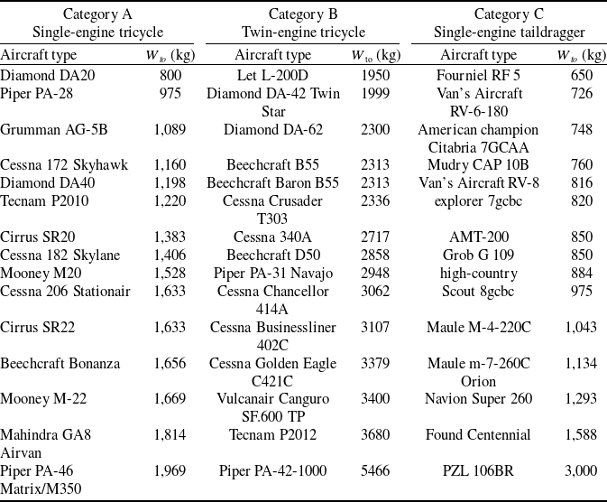
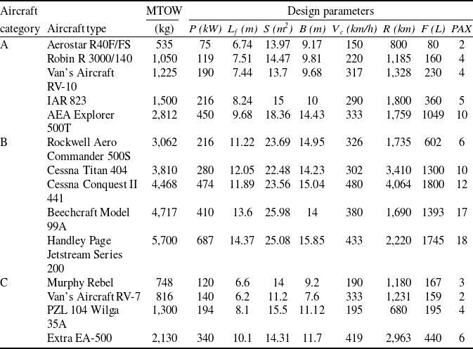
Additionally, only piston-engine aircraft with identical design characteristics and features are considered. All-electric aircraft are becoming more popular, but for the foreseeable future, internal combustion engines will still be employed in design and production. Three categories, single-engine tricycle (Category A), double-engine tricycle (Category B) and single-engine taildragger (Category C), are utilised to classify the sampled data (aircraft) used in modelling and testing. The aircraft mentioned in Table 2 are utilised to establish the weight-predicting models.
The aircraft categories with their MTOW

In exploring the aircraft listed in Table 2, it is noted that both conventional and composite aircraft are represented. In contrast, because there are only a handful of certified electric aircraft, all of which are very new, they are also omitted. Therefore, the design variables must be general; more specifically, they must not be technology-specific.
However, a typical collection of variables has been selected to build the weight-predicting models [Reference Al-Shamma and Ali16]. The chosen variables used in this study were determined, predicted or known at the conceptual design stage and have a significant impact on practically all design and weight-prediction aspects. These design variables include aircraft length (L f ), wing area (S), wingspan (b) and number of passengers (PAX) from the geometry section; aircraft cruise speed (V c ) and range (R) from the performance section; as well as engine power (P) and fuel capacity (F) from the propulsion section.
3.1 Multicollinearity problem
Multicollinearity in regression arises when two or more independent variables are highly correlated, thereby violating the assumption of independence among predictors. One desirable attribute of regression is the isolation and quantification of the individual effect of each independent variable on the dependent variable, associated with a one-unit change in each independent variable whilst holding all other independent variables constant. When multicollinearity is present, it becomes difficult to interpret the results because the independent variables are highly correlated.
Multicollinearity gives rise to two principal issues. First, it inflates the variance of the estimated coefficients, reducing their precision and, consequently, diminishing the model’s statistical power. This leads to unreliable p-values and undermines the identification of statistically significant independent variables. Second, the estimated coefficients become unstable and highly sensitive to small changes in the model, producing substantial fluctuations in coefficient magnitude and even sign, reflecting an inherent lack of robustness in the estimates [Reference Hayes and Scott17].
Whether multicollinearity needs to be addressed depends on how severe it is and on what the model is being used for. Several considerations, as outlined in Ref. [Reference Forest18], are worth examining. As the degree of multicollinearity increases, its detrimental effects become more pronounced; however, at moderate levels, corrective action may not be necessary. Moreover, multicollinearity primarily affects those variables that are strongly correlated, and if such variables are not of substantive interest, intervention may be unnecessary. Importantly, multicollinearity does not materially affect overall quality-of-fit measures or predictive accuracy; rather, its effect is confined to the estimation of individual coefficients.
Diagnostic evaluation of multicollinearity typically involves examining pairwise correlations among independent variables and computing the variance inflation factor (VIF). These techniques are widely implemented in statistical software packages, including Microsoft Excel. A VIF value of 1 indicates no correlation between the independent variables under consideration and the remaining independent variables. Values between 1 and 5 suggest moderate correlation that is generally acceptable, whereas values exceeding 5 indicate potentially problematic multicollinearity. In such cases, coefficient estimates are likely to be inaccurate, and p-values unreliable, and phenomena such as sign reversals and inflated standard errors may arise, as stated before.
The VIF can be calculated in Excel by exploiting its definition rather than relying on a built-in function. For each independent variable ${X_i}$
, a separate (auxiliary) regression is performed in which
${X_i}$
, a separate (auxiliary) regression is performed in which ${X_i}\;$
is treated as the dependent variable, and all remaining independent variables are used as independent variables. Using Excel’s Data Analysis ToolPak, this regression yields an
${X_i}\;$
is treated as the dependent variable, and all remaining independent variables are used as independent variables. Using Excel’s Data Analysis ToolPak, this regression yields an ${R^2}$
value, which indicates how well
${R^2}$
value, which indicates how well ${X_i}\;$
is explained by the other independent variables. The VIF is then computed using the standard relationship [Reference Shrestha19]:
${X_i}\;$
is explained by the other independent variables. The VIF is then computed using the standard relationship [Reference Shrestha19]:
 \begin{align}VI{F_i} = \frac{1}{{1 - R_i^2}}\end{align}
This process is repeated for each independent variable in the model. A VIF value of 1 indicates no multicollinearity, while values between 1 and 5 suggest moderate correlation that is often acceptable in practice. Values exceeding 5 – and particularly above 10 – indicate increasingly severe multicollinearity, which leads to inflated standard errors, unstable coefficient estimates and unreliable statistical inference. Although Excel requires this iterative approach, the method is entirely consistent with standard statistical practice [Reference Montgomery, Peck and Vining20], which provides formal guidance on diagnosing and interpreting multicollinearity in regression models.
4.0 The proposed approach and model development
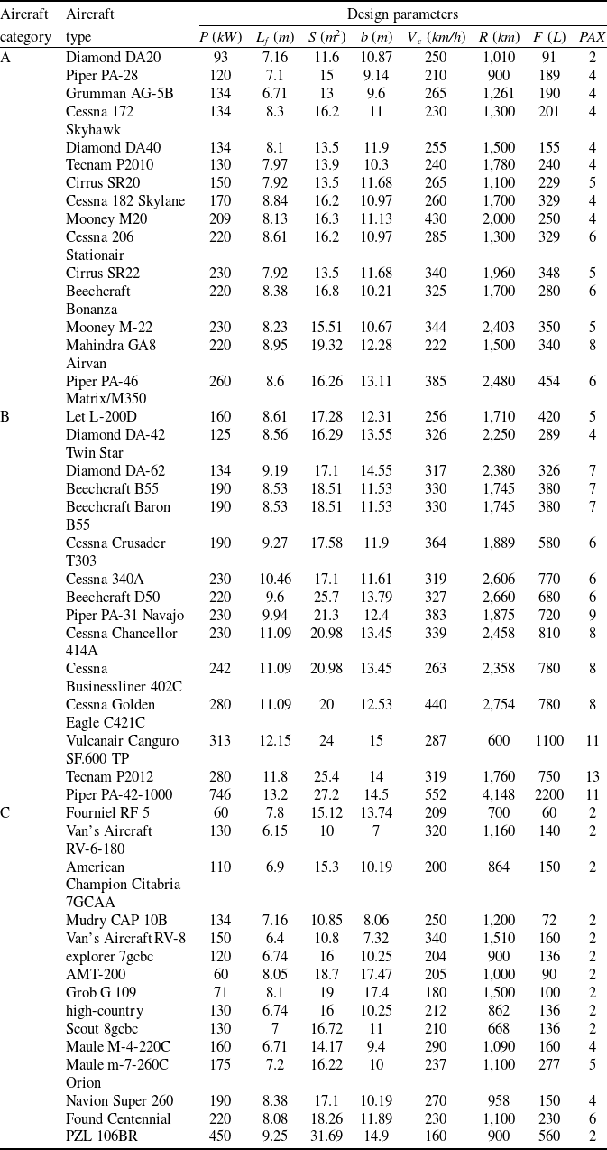
The data used to establish the empirical models have been extracted from the web, manufacturers’ technical specifications, pilot operating handbooks, FAA-type certificates, manufacturer performance charts, flight test reports, aviation databases and aircraft design textbooks, to name a few. Data from these sources have been compiled in Table 1 for the MTOW and in Table 2 for the main design variables.
This work developed three models to estimate the aircraft MTOW using multiple linear regression, in conjunction with p-value analysis, which is used to reduce the set of independent variables to a minimum while maintaining high estimation accuracy. This reduction in variables in the resulting model may speed up decision-making, highlight the importance of parametric analysis and make it easier to estimate aircraft MTOW. The p-values for the regression model coefficients can also be used to assess the significance of each design variable. In other words, if the p-value is high, the parameter significance is low, and vice versa. It is inversely proportional to the p-value.
To perform the MLR, several statistical platforms and software are available on the market. This work used the most popular software, MS Excel. It has several built-in data analysis tools, as part of the Analysis ToolPak, such as correlation, regression and t-test. To access the regression tool, select the Data tab from the home page, then select the Data analysis tab from the Analyse section. Finally, select the regression tool from the opening list window.
Note that successful use of MLR requires that the total number of dependent and independent parameters be less than the number of aircraft in the category, by at least 1. Thus, no more than 14 independent variables can be chosen. Alternatively, correlation analysis is used first to minimise the number of independent parameters by eliminating those with the lowest correlation coefficients. In Section 3, the total number of design variables (independent parameters) is 8, plus the dependent parameter (MTOW variable in this study). Moreover, all categories (A, B, and C) have 15 aircraft. Therefore, there is no need to apply the correlation analysis to minimise the number of independent parameters.
The input values of the design variables

Based on the aircraft in Table 2, Table 3 provides the input values of the design variables for each aircraft in the three aircraft categories. Starting with Category A, the mathematical model of the estimated MTOW can be extracted from the MLR output as mentioned in Section 2.1:
 \begin{align}{W_{to.est\;\left[ {cat.\;\;A} \right]}} = 120.9809 \times PAX + 97.22259 \times {L_f} + 8.990606 \times b - 16.2701 \times S + 0.571669 \times P \nonumber\\ + 1.317788 \times {V_c} + 0.067629 \times R + 0.661598 \times F - 564.382\end{align}
Similarly, the mathematical models for Categories B and C are:
 \begin{align}{W_{to.est\;\left[ {cat.\;\;B} \right]}} = 51.77997 \times PAX + 221.1475 \times {L_f} - 7.04112 \times b + 37.58779 \times S + 2.923553 \times P \nonumber\\ + 1.05773 \times {V_c} + 0.151307 \times R - 0.33279 \times F - 1600.58\end{align}
 \begin{align}{W_{to.est\;\left[ {cat.\;\;C} \right]}} = 21.45537 \times PAX - 25.1091 \times {L_f} + 57.37207 \times b + 5.397891 \times S + 6.395582 \times P \nonumber\\ + 0.44584 \times {V_c} + 0.09982 \times R + 0.46689 \times F - 430.84\end{align}
Note that the MLR analysis considered all the independent variables. To reduce the number of independent variables to the minimum possible while keeping the error accuracy within the desired range, p-value analysis is considered. This analysis performs the MLR analysis in an iterative procedure. At the end of each iteration, the design variable with the highest p-value is removed from the regression parameter list. The iterative procedure ends once all p-values fall below 0.05. The final model is obtained using the remaining variables.
Thus, in considering Category A, the P parameter, which had the highest p-value, was eliminated after the first MLR execution, and the b parameter was eliminated after the second. Hence, the final mathematical formula is:
 \begin{align}{W_{to.est\;\left[ {cat.\;\;A} \right]}} = 0.721811 \times F + 111.4565 \times {L_f} + 1.504516 \times {V_c} + 133.9247 \times PAX \nonumber\\ + 0.081801 \times R - 20.1199 \times S - 573.377\end{align}
Similarly, in Category B, the b and F parameters were eliminated. The final mathematical formula is:
 \begin{align}{W_{to.est\;\left[ {cat.\;\;B} \right]}} = 176.3897 \times {L_f} + 33.60172 \times S + 2.054176 \times P + 1.046836 \times {V_c} \nonumber\\ + 0.172823 \times R + 69.59588 \times PAX - 1360.57\end{align}
And, in Category C, the S, L f , F and V c parameters were eliminated. The final mathematical formula is:
 \begin{align}{W_{to.est\;\left[ {cat.\;\;C} \right]}} = 50.75259 \times b + 5.888885 \times P + 19.50779 \times PAX - 0.07986 \times R - 365.99\end{align}
In Category A, it should be noted that the wing area coefficient has a negative sign (Equation (9)), whereas the variable itself has a strong relationship with the MTOW. The wing area variable also has strong correlations with PAX, length, engine power and fuel capacity. Thus, it works here as a suppressor variable. It effectively removes from the model the part of the independent variable that does not relate to the outcome. Physically, as the wing area increases, the lift force increases, and the climb stage time is reduced. Hence, fuel consumption decreases, and the total fuel capacity is reduced. Thus, the MTOW is decreased. Similarly, in Category C, the range variable has a strong relationship with the cruise speed variable (see Equation (11)), and it also acts as a suppressor variable.
Note that the E-Conditions of the CAA requirements for experimental aircraft [21] cover the aircraft whose MTOW is less than 2,000 kg. Most aircraft in Categories A and C are below this limit. In general, models (Equations (6), (7) and (8)) or shorter ones (Equations (9), (10) and (11)) can help predict MTOW for aircraft specifically under 6,000 kg.
5.0 Results and discussion
The established models (Equations (6), (7) and (8), using MLR analysis, and Equations (9), (10) and (11), using MLR + p-value analysis) were used to estimate the MTOW for all categories. Figure 2 shows the actual and estimated MTOW for each category.
The actual and estimated MTOW for Categories A, B and C.

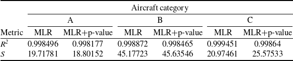
Initially, it is important to evaluate the fitness of the MLR models (Equations (6), (7) and (8)) and the short models (Equations (9), (10) and (11)), as mentioned in Section 2.1.2. Thus, the metrics R 2 and S were extracted from the MLR output and listed in Table 4. The R2 values are above 99.8% for all models and are very close to 1, indicating that the data fit very well with very small error. Regarding the second metric S, the values are 19.72 and 18.8 for the two Category A models, respectively. When comparing this metric to the average dependent variable (MTOW = 1,408 kg), it corresponds to 1.4% and 1.33% for both models, respectively. These values ensure that the data fit the model well and that the error is very low (less than 1.5%). Similarly, the average MTOW is 2,921 kg for Category B, and the S values are 45.18 and 45.64, representing 1.55% and 1.56%, respectively. For Category C, the mean MTOW is 1,075 kg, and the S values are 20.97 and 25.58, corresponding to 1.95% and 2.38%. Thus, the error accuracy is slightly higher than that of Category A and Category B, but it is still highly acceptable (less than 2.5%)
The fitness evaluation metrics of the MLR models for all categories

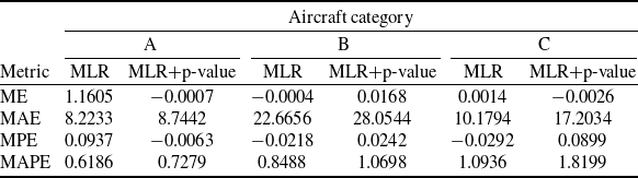
On the other hand, numerous metrics are available in statistical analysis to assess how well the empirical weight-estimation models work. The mean error (ME), the average of the differences between estimated and actual values, is one of these metrics. In addition, the mean percentage error (MPE) is the average of the percentage variations. Bear in mind that these variations might have positive or negative values and could even cancel each other out. As a result, weight estimation may be used as a biased metric. Another metric known as the mean absolute error (MAE) is the absolute difference between the estimated and actual values. Because it is convenient and straightforward, a commonly used metric for model evaluation is the mean absolute percentage error (MAPE). The values of these metrics applied to all categories are shown in Table 5.
The metrics’ values for all categories

In examining the first metric (ME) for Category A, it is very low (less than 1 g), while the MAE is high (more than 8 kg). These values indicate that the positive samples approximately equal the negative ones (+ eats −). For Categories B and C, ME and MAE behave similarly to those in Category A, but with proportionally higher values. In general, the MAE is slightly less than half the regression standard error (S). Investigating the values of the third and fourth metrics (MPE and MAPE) shows behaviour similar to that of ME and MAE, respectively. Thus, these metrics are not useful for achieving model accuracy.
However, to better assess the model error, the difference between the actual and estimated values (using Equations (6)–(11)), known as the error (Error), and the percentage error (Error %) were computed. Figure 3 shows the error percentage (Error %) for both models (MLR and MLR+p-value) across the three categories. In considering Category A, the MLR model has a range of error between −1 to 2 %, while the MLR + p-value model has an error range between −2 and >3 %. Therefore, the MLR is a more accurate model. In Category B, both models are close, with a slight preference for the MLR model. The performance of Category C is similar to Category A. Thus, MLR is obviously the winner.
Next, the minimum and maximum percentage error (Error %) values for all models were extracted. Finally, the greater of the two absolute values is considered the model error accuracy (MEA). These findings for the three categories are presented in Table 6.
The summary of model error accuracy (MEA)

Model error accuracy % for all categories.

From Table 6, the MLR models achieve error accuracies below 3% for all categories, while the short models (MLR + p-value) have error accuracies below 5%. These findings significantly enhance MTOW estimation at early stages compared to traditional textbook methods, whose accuracy is between 5–10%.
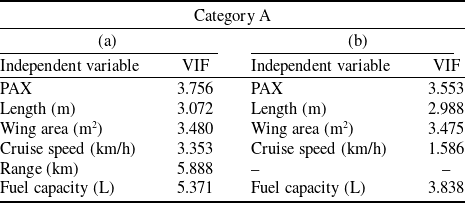
As discussed in Section 3, the variables selected for this study are defined at the conceptual design stage and primarily influence both configuration and weight estimation; accordingly, a degree of interdependence among the independent variables is expected. Multicollinearity was initially assessed using correlation analysis. For Category A, strong pairwise correlations were identified across geometric (e.g. PAX–length, PAX–wing area, length–wing span, length–wing area), performance (e.g. power–cruise speed, power–range, power–fuel, cruise speed–range, range–fuel) and mixed configurations (e.g. PAX–power, PAX–fuel, length–power, length–fuel, wing area–fuel).
To reduce redundancy, wingspan and engine power were removed during refinement of the MLR + p-value model. VIFs were subsequently computed to quantify the remaining multicollinearity. Most independent variables exhibited moderate VIF values; however, two variables marginally exceeded the commonly accepted threshold of 5 (remaining below 6), as shown in Table 7. Removal of the variable with the highest VIF reduced all remaining VIF values to 1–5, indicating acceptable levels of multicollinearity. This refinement also led to a modest improvement in model performance, with the prediction error remaining below 5%.
The VIF values for the MLR+p-value variables (a) before (b) after solving multicollinearity problem

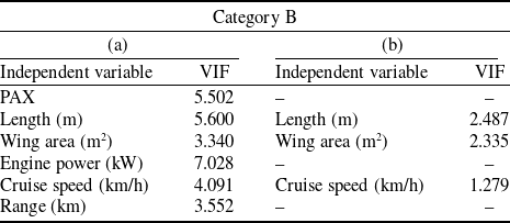
Application of the correlation analysis to Category B revealed multiple strong relationships across geometric (PAX–length, PAX–wing area, length–wing area), performance (power–cruise speed, power–fuel, cruise speed–range, cruise speed–fuel) and mixed configurations (PAX–power, PAX–fuel, length–power, length–fuel, wing area–power, wing area–fuel).
In forming the MLR + p-value model, wingspan and fuel were initially removed. Subsequent evaluation using VIFs indicated severe multicollinearity associated with the fuel variable, marginally severe levels for PAX and length and moderate levels for the remaining independent variables – reapplication of the p-value criterion led to the exclusion of PAX, power and range.
The final model, comprising length, wing area and cruise speed, exhibits low to moderate multicollinearity (see Table 8). However, consistent with Category A, this refinement results in a deterioration in model accuracy, with the prediction error approximately doubling to exceed 5%.
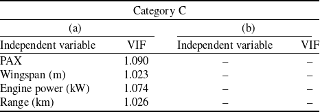
Similarly, Category C exhibits several strong correlations among the independent variables. Within the geometric configuration, notable relationships exist among length–wingspan, length–wing area and wingspan–wing area. In the performance configuration, strong correlations are observed between power–fuel and cruise speed–range, while mixed interactions include wing area–power and wing area–fuel.
To address multicollinearity, an initial variable reduction was performed within the MLR + p-value framework, resulting in the removal of wing area, length, fuel and cruise speed. VIFs were subsequently evaluated for the remaining independent variables. All variables had VIF values of 1, indicating no multicollinearity (see Table 9). Accordingly, no further corrective action was required.
The VIF values for the MLR+p-value variables (a) before (b) after solving multicollinearity problem

The VIF values for the MLR+p-value variables (a) before (b) after solving multicollinearity problem

Lastly, it can be concluded that reducing the impact of multicollinearity requires removing one or more of the correlated independent variables, which enhances the reliability and stability of the resulting model but may increase the error rate, potentially doubling that of the MLR+p-value model.
6.0 Case studies
Evaluating the proposed method requires testing additional aircraft to certify their suitability. In Categories A and B, five aircraft were employed (not used in building the estimation models), and a further four aircraft were utilised for Category C due to the limited number of available aircraft. Moreover, the conditions still ‘in service’ and/or ‘in production’ are also applied. Table 10 presents these aircraft and their design parameter values.
The design parameter values (case studies aircraft)

For all categories, Equations (6)–(11) were used to estimate the aircraft MTOW. Figure 4 presents the actual and estimated MTOW, using MLR and MLR+p-value techniques. It is clearly demonstrated that the estimated findings from both techniques are very close to the actual MTOWs.
The actual and estimated MTOW for the tested aircraft of all categories.

Consequently, to determine the accuracy of the tested aircraft’s error precisely, the difference (Error) and the percentage difference (Error %) were also calculated. Figure 5 shows the error accuracy of each tested aircraft for all categories. The graphs showed that the error was less than 5% across all categories for both the long and short formulae.
The tested aircraft error accuracy % for all categories.

The impact of the variables for the full and short models of Category A.

However, according to many textbooks, early in the design process, it is acceptable for the estimated MTOW to be within 10% of the target value. The developed models (Equations (6)–(8) and (9)–(11)) enable designers to estimate the MTOW of new designs with an error accuracy of less than 5%. The weight estimates obtained with the test aircraft confirm the applicability of the developed models and facilitate parametric analyses based on key design variables.
7.0 Parametric studies
However, an impartial evaluation is required to evaluate the sensitivity of the created models. Because of the model’s linearity, MTOW estimation is easily done. Additionally, it makes parametric studies easier by allowing the design parameters to be used to determine the sensitivity and effect of changes. Every parameter coefficient has an effect. The largest coefficient corresponds to the greatest effect, and vice versa. Furthermore, a crucial factor in identifying the direction of proportionality is the sign of the coefficient. If the sign is positive, the predicted MTOW is directly proportional; if the sign is negative, inverse proportionality is indicated. For example, the Category A short model (Equation (9)) contains all positive (directly proportional) coefficients except the S parameter (F, L f , V c , PAX and R). Furthermore, since the PAX parameter has the largest coefficient, it has the greatest impact. While adding 1 m to the aircraft length would raise the MTOW by just 111 kg, reducing one passenger would result in 133 kg of MTOW savings. Logically, adding 1 litre of fuel will increase MTOW by 0.7 kg.
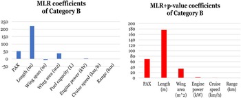
In considering the MLR model (Equation (10)) for Category B, the aircraft length has the largest coefficient, since adding 1 m will increase the MTOW by 221 kg, whereas decreasing the wing area by 1 m2 will save 37.5 kg. The range parameter has the lowest coefficient value and the least influence (see Fig. 7).
The impact of the variables for the full and short models of Category B.

Finally, the short model (Equation (11)) of Category C has only four parameters: b, P, PAX and R. The Span coefficient is the highest, and increasing it by 1 m will increase the MTOW by 50 kg. Similar to Category B, the Range coefficient has the lowest impact on the MTOW (see Fig. 8).
The impact of the variables for the full and short models of Category C.

8.0 Conclusion
Multilinear regression, alone and in combination with p-value analysis as parametric weight estimation techniques, was introduced in this paper to estimate the MTOW of extremely light aircraft. Utilising aircraft (dataset samples) that are still ‘in production’ and/or ‘in service’, empirical models were created. They fall into one of three categories based on the arrangement of their landing gear and the number of engines. In addition, the aircraft design is heavily influenced by the selection of eight crucial design parameters, which in turn impact the final aircraft MTOW. The results demonstrated that, with an error accuracy of less than ±5 %, the generated models could successfully predict the MTOW during the preliminary design phases. This accuracy is the highest among the weight-estimation techniques currently available, and it enables parametric studies that include important design parameters during the early design stage.








 Open access

