


1. Introduction
Answering many questions in macro and labor economics requires modeling of the individual and household income dynamics. It is common to posit a model of log-idiosyncratic income as a sum of long-lasting and transitory components and a fixed effect. Due to its relative simplicity and wide applicability, such an income process is often labeled as the canonical income process; for example, Arellano et al. (Reference Arellano, Blundell and Bonhomme2017).
There are various approaches to estimating the income process parameters. The literature typically relies on a minimum-distance estimation and autocovariance moments of log-income levels, $y_{it}$
, or differences,
$y_{it}$
, or differences, $\Delta y_{it}=y_{it}-y_{it-1}$
; see, for example, Daly et al. (Reference Daly, Hryshko and Manovskii2022) for a discussion. The objective of this paper is to provide a guide to estimating the canonical income process using quasidifferences defined as
$\Delta y_{it}=y_{it}-y_{it-1}$
; see, for example, Daly et al. (Reference Daly, Hryshko and Manovskii2022) for a discussion. The objective of this paper is to provide a guide to estimating the canonical income process using quasidifferences defined as $\tilde{\Delta }y_{it}=y_{it}-\rho y_{it-1}$
, where
$\tilde{\Delta }y_{it}=y_{it}-\rho y_{it-1}$
, where $\rho$
is the persistence of shocks to the long-lasting component.
$\rho$
is the persistence of shocks to the long-lasting component.
Estimations in levels, differences, and quasidifferences have their advantages and disadvantages. Estimation in levels can recover the variance of fixed effects but requires a stand on the distribution of fixed effects and initial conditions and can be cumbersome to implement if the shocks’ variances change with time and age. Estimation in differences is preferable when the long-lasting component is a random walk since fixed effects and initial conditions get differenced out and do not affect the estimated parameters. However, even though there is a consensus that the shocks to the long-lasting component are persistent, the literature is far from the consensus that these shocks are permanent. If one departs from assuming that the long-lasting component is a random walk, estimation in differences loses its advantages relative to estimation in levels. Estimation in quasidifferences inherits the advantages of estimation in levels and differences. Like estimation in differences when the long-lasting component is a random walk, it is not dependent on the distribution of initial conditions and is easy to implement. In quasidifferences, this is true even if the shocks to the long-lasting component are not permanent. Like estimation in levels, it allows for estimation of the variance of fixed effects. The challenging aspect of estimation in quasidifferences, however, is the requirement of an estimate of the persistence. In principle, estimation could proceed in two stages: first, estimation of the persistence, and second, estimation of the other parameters of the income process. Persistence could be estimated by GMM, which, like estimation in levels, requires modeling of the initial conditions.Footnote
1
To overcome this challenge, Blundell et al. (Reference Blundell, Graber and Mogstad2015) proposed recently to jointly estimate the persistence and the other income process parameters using quasidifferences. The procedure they suggest involves the evaluation of the distance between the model and the data autocovariance moments for a predefined grid in persistence and choosing the set of the income process parameters that minimizes the distance as the model estimates. Although this procedure is appealing in its simplicity and merits relative to the estimations in levels and differences, nothing is known about its performance in realistic settings. Using Monte Carlo simulations, our paper is the first to conduct such an analysis and examine the biases in the estimated parameters using quasidifferences for various true values of the persistence, $N$
,
$N$
, $T$
, initial conditions, and weighting schemes.
$T$
, initial conditions, and weighting schemes.
Following a large GMM literature,Footnote 2 our primary focus is on evaluating the biases in the estimates of persistence, but we also catalog the results for the other parameters in the appendix. Precise estimation of the persistence is important for the design of the optimal tax policy as highlighted in Farhi and Werning (Reference Farhi and Werning2012) and for the interpretation of transmission coefficients for long-lasting income shocks to household consumption as emphasized in Blundell (Reference Blundell2014), Hryshko and Manovskii (Reference Hryshko and Manovskii2022) and Bryukhanov and Hryshko (Reference Bryukhanov and Hryshko2020).Footnote 3 Footnote 4 Blundell et al. (Reference Blundell, Graber and Mogstad2015) measure the persistence of long-lasting shocks to male earnings, male and family disposable income to evaluate the insurance role of the tax and transfer system and family labor supply in moderating the persistence of longer-lasting shocks to male earnings. We find that equally weighted estimation often results in downward-biased estimates of the persistence in small and large samples regardless of the magnitude of true persistence. The bias is bigger, ceteris paribus, when the variance of fixed effects is smaller, the variance of persistent shocks is smaller, or the variance of transitory shocks is higher. Only when the variance of persistent shocks is bigger than the variance of transitory shocks equally weighted estimation is reliable in recovering the true values of the persistence. This is the setting of Blundell et al. (Reference Blundell, Graber and Mogstad2015), who used equally weighted estimation and very big samples from administrative Norwegian data on earnings and incomes. Optimal and diagonal weighting produce nontrivial upward biases in the estimated persistence when the true persistence is low and the variance of incomes in the first sample year is nonnegligible—this may happen either when the average age of individuals in the first sample year is sufficiently large (due to accumulation of persistent shocks) or when the variance of initial conditions is nonnegligible. Similar to equal weighting, optimal and diagonal weighting produce unbiased estimates of the persistence when the variance of long-lasting shocks is bigger than the variance of transitory shocks but only when the variance of the persistent component in the first sample year is small (e.g., when following a cohort of individuals from the start of their working careers).
Other applications require precise estimates of the variance of persistent and transitory shocks and fixed effects. The variance of long-lasting shocks, for example, is an important driver of wealth accumulation in a buffer-stock model of saving (Carroll (Reference Carroll1997)), whereas the variance of fixed effects determines if inequality is important for the determination of the aggregate demand (Auclert and Rognlie (Reference Auclert and Rognlie2018)). Using quasidifferences, we find that the variance of fixed effects is severely upward-biased when the true persistence is high, but the biases in its estimation are small when the true persistence is low. The variances of persistent and transitory shocks are estimated with small biases, especially when the number of sample individuals is large.
In an empirical application, we use administrative data on earnings for a large sample of Danish males born in 1952 observed during the 1984–2008 period to estimate the canonical income process using quasidifferences. We find that the variance of transitory shocks is about twice as large as the variance of persistent shocks and that optimal weighting of the moments yields a relatively high estimate of the persistence followed by smaller estimates when using a diagonal and equal weighting of the moments. We next estimate the income process using small bootstrap samples out of the original sample of Danish males. Optimal weighting produces a relatively stable estimate of the persistence in large and small samples, whereas diagonal weighting results in a substantially higher estimate of the persistence in small samples, and equal weighting yields a smaller estimate in small samples. These results agree with our results for large and small samples from simulated data generated for high persistence of long-lasting shocks when the variance of transitory shocks is higher than the variance of persistent shocks and the variance of the persistent component in the initial sample year is nonnegligible (due to a history of accumulation of persistent shocks or nonzero initial conditions).
Estimation in quasidifferences is amenable to the methodology of Blundell et al. (Reference Blundell, Pistaferri and Preston2008) that aims to recover, besides the income process parameters, the transmission of long-lasting and transitory shocks to household consumption, that is, the fraction of long-lasting and transitory shocks that are absorbed by consumption. It generalizes the original methodology due to its potential to recover the persistence of long-lasting shocks that may differ from unity and the variance of fixed effects in household incomes. Our analysis of the income-process estimation in quasidifferences recovers the variance of persistent and transitory shocks nearly without biases but produces biased estimates of persistence in balanced panels. These results, if maintained within the methodology of Blundell et al. (Reference Blundell, Pistaferri and Preston2008), would raise the issue of interpretation of the extent of consumption insurance even if it was estimated without a bias. To explore the effectiveness of estimation in quasidifferences using consumption and income data, we calibrate a standard incomplete-markets model for low and high values of persistence and simulate the data replicating the age structure of data from the Panel Study of Income Dynamics (PSID) used in Hryshko and Manovskii (Reference Hryshko and Manovskii2022). We find significant biases both in the estimated persistence and the transmission coefficients for persistent and transitory shocks for high and low values of persistence, different weighting schemes, and the number of households in the simulated data.
The results in our paper warn against the routine use of estimation in quasidifferences despite its attractive features. However, there is one case when estimation in quasidifferences reliably recovers the persistence of long-lasting shocks. When the variance of persistent shocks is higher than the variance of transitory shocks, equally weighted estimation recovers the true persistence of long-lasting shocks for different $T$
,
$T$
, $N$
, and initial conditions. Since biases in the variances of the shocks using estimation in quasidifferencs are small, our advice is to estimate the income process using equal weighting of the moments and use the results with confidence if the estimated variance of persistent shocks is higher than the variance of transitory shocks.
$N$
, and initial conditions. Since biases in the variances of the shocks using estimation in quasidifferencs are small, our advice is to estimate the income process using equal weighting of the moments and use the results with confidence if the estimated variance of persistent shocks is higher than the variance of transitory shocks.
The rest of the paper is structured as follows. In Section 2, we present theoretical moments in levels, differences, and quasidifferences for the canonical income process and discuss the identification and estimation of the income-process parameters. In Section 3, we present the details of our Monte Carlo simulations, and in Section 4, we present the results of estimations in quasidifferences using the simulated data. Section 5 analyzes the bias in the estimated persistence using simulated income data, presents the results from an empirical application using administrative data on earnings from Denmark, and analyzes the bias in the income- and consumption-process parameters using data from a calibrated lifecycle model of consumption. Section 6 discusses the implications of our results for practical use, and Section 7 concludes.
2. The canonical income process
We consider the canonical decomposition of idiosyncratic (log-)income for individual $i$
at time
$i$
at time $t$
,
$t$
, $y_{it}$
, into a sum of an autoregressive component
$y_{it}$
, into a sum of an autoregressive component $z_{it}$
, fixed effect
$z_{it}$
, fixed effect $\alpha _i$
, and transitory shock
$\alpha _i$
, and transitory shock $\epsilon _{it}$
:
$\epsilon _{it}$
:
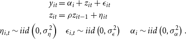 \begin{align} y_{it} & = \alpha _{i} + z_{it}+\epsilon _{it} \nonumber \\ z_{it} & = \rho z_{it-1}+\eta _{it}\\ \eta _{i,t} \sim{iid}\left(0, \sigma ^{2}_{\eta }\right) & \quad \epsilon _{i,t} \sim{iid}\left(0, \sigma ^{2}_{\epsilon }\right) \quad \alpha _{i} \sim{iid}\left(0, \sigma ^{2}_{\alpha }\right). \nonumber \end{align}
Shocks $\eta _{it}$
have persistence
$\eta _{it}$
have persistence $\rho$
, all shocks and the fixed effect are i.i.d. and are orthogonal to each other. In quantitative macro, it is common to assume that the initial condition
$\rho$
, all shocks and the fixed effect are i.i.d. and are orthogonal to each other. In quantitative macro, it is common to assume that the initial condition $z_{i0}$
takes the value of zero for everyone, whereas in the panel-data literature, the initial condition is commonly assumed to be drawn from some distribution. We will consider both of these assumptions in our Monte Carlo simulations.
$z_{i0}$
takes the value of zero for everyone, whereas in the panel-data literature, the initial condition is commonly assumed to be drawn from some distribution. We will consider both of these assumptions in our Monte Carlo simulations.
2.1 Theoretical moments
Assuming that initial conditions $z_{i0}$
are i.i.d. and orthogonal to the shocks and fixed effects, the autocovariance function of incomes in levels, differences, and quasidifferences for a cohort of individuals who start their working life at time 0 can be characterized as follows.
$z_{i0}$
are i.i.d. and orthogonal to the shocks and fixed effects, the autocovariance function of incomes in levels, differences, and quasidifferences for a cohort of individuals who start their working life at time 0 can be characterized as follows.
Levels:
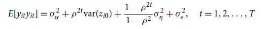 \begin{align} E[y_{it}y_{it}]&=\sigma ^2_{\alpha }+\rho ^{2t}\hbox{var}(z_{i0})+\frac{1-\rho ^{2t}}{1-\rho ^2}\sigma ^2_{\eta }+\sigma ^2_{\epsilon },\quad t=1, 2,\ldots, T\qquad\qquad\qquad\qquad \end{align}
 \begin{align} E[y_{it+k}y_{it}]&=\sigma ^2_{\alpha }+\rho ^k\left [\rho ^{2t}\hbox{var}(z_{i0})+\frac{1-\rho ^{2t}}{1-\rho ^2}\sigma ^2_{\eta }\right ],\quad t=1, 2,\ldots, T-k;\quad 1\leq k\leq T-t. \end{align}
Differences:
 \begin{align} E[\Delta y_{it}\Delta y_{it}]&=\rho ^{2(t-1)}(1-\rho )^2\hbox{var}(z_{i0})+\left [1+\frac{1-\rho }{1+\rho }\left (1-\rho ^{2(t-1)}\right )\right ]\sigma ^2_{\eta }+2\sigma ^2_{\epsilon },\quad t=2,\ldots, T \end{align}
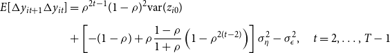 \begin{align} E[\Delta y_{it+1}\Delta y_{it}]&=\rho ^{2t-1}(1-\rho )^2\hbox{var}(z_{i0})\nonumber\\[5pt]& +\left [-(1-\rho )+\rho \frac{1-\rho }{1+\rho }\left (1-\rho ^{2(t-2)}\right )\right ]\sigma ^2_{\eta }-\sigma ^2_{\epsilon },\quad t=2,\ldots, T-1 \end{align}
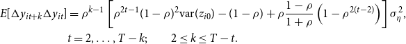 \begin{align} E[\Delta y_{it+k}\Delta y_{it}]&=\rho ^{k-1}\left [\rho ^{2t-1}(1-\rho )^2\hbox{var}(z_{i0})-(1-\rho )+\rho \frac{1-\rho }{1+\rho }\left (1-\rho ^{2(t-2)}\right )\right ]\sigma ^2_{\eta },\notag \\ &t=2,\ldots, T-k;\quad \quad 2\leq k\leq T-t. \end{align}
Quasidifferences:
 \begin{align} &\notag \\ E[\Delta \tilde{y}_{it}\Delta \tilde{y}_{it}]&=(1-\rho )^2\sigma ^2_{\alpha }+\sigma ^2_\eta +(1-\rho )^2\sigma ^2_\epsilon,\quad t=2,\ldots, T \end{align}
 \begin{align} E[\Delta \tilde{y}_{it+1}\Delta \tilde{y}_{it}]&=(1-\rho )^2\sigma ^2_\alpha -\rho \sigma ^2_\epsilon,\quad \quad \quad \quad \quad t=2,\ldots, T-1 \end{align}
 \begin{align} E[\Delta \tilde{y}_{it+k}\Delta \tilde{y}_{it}]&=(1-\rho )^2\sigma ^2_\alpha,\quad \quad \quad \quad \quad \quad \quad t=2,\ldots, T-k;\quad 2\leq k\leq T-t. \end{align}
2.2 Identification and estimation
Identification of the income process parameters in equation (1) is typically established by using the moments involving combinations of autocovariances of income in levels or differences, whereas estimation is commonly performed relying on the minimum-distance method that involves matching all available autocovariance moments of incomes in levels or differences to their theoretical counterparts; see, for example, Meghir and Pistaferri (Reference Meghir and Pistaferri2004), Heathcote et al. (Reference Heathcote, Perri and Violante2010), and Daly et al. (Reference Daly, Hryshko and Manovskii2022).
There are advantages and disadvantages of estimations relying on the moments in levels or differences. Estimation in differences is the most obvious choice if the autoregressive component is a random walk, $\rho =1$
, as it is valid for various distributions of the initial conditions for the persistent component and fixed effects. However, it does not allow for the identification of the variance of fixed effects; they are differenced out. Estimation in levels, in turn, requires making a stand on the distribution of initial conditions for the autoregressive component, as we have done at the start of Section 2.1. Our focus is on recovering the model parameters using quasidifferences defined as
$\rho =1$
, as it is valid for various distributions of the initial conditions for the persistent component and fixed effects. However, it does not allow for the identification of the variance of fixed effects; they are differenced out. Estimation in levels, in turn, requires making a stand on the distribution of initial conditions for the autoregressive component, as we have done at the start of Section 2.1. Our focus is on recovering the model parameters using quasidifferences defined as $\tilde{\Delta } y_{it}=y_{it} -\rho y_{it-1}$
. The moments in equations (7)–(9) are much simpler than the levels and differences moments in equations (2)–(6): they do not vary with
$\tilde{\Delta } y_{it}=y_{it} -\rho y_{it-1}$
. The moments in equations (7)–(9) are much simpler than the levels and differences moments in equations (2)–(6): they do not vary with $t$
and
$t$
and $k$
and allow for the identification of only three out of four unknown parameters—fixing
$k$
and allow for the identification of only three out of four unknown parameters—fixing $\rho$
enables identification of the variance of fixed effects and the variances of persistent and transitory shocks.Footnote
5
Thus, although this method inherits the simplicity of estimation in differences when the autoregressive component is a random walk and allows for estimation of the variance of fixed effects, it requires an estimate of the persistence,
$\rho$
enables identification of the variance of fixed effects and the variances of persistent and transitory shocks.Footnote
5
Thus, although this method inherits the simplicity of estimation in differences when the autoregressive component is a random walk and allows for estimation of the variance of fixed effects, it requires an estimate of the persistence, $\rho$
.
$\rho$
.
How would one obtain a reliable estimate of the persistence? One possibility is to use GMM. Similar to the minimum-distance estimation in levels, GMM requires modeling initial conditions. It can also be substantially biased in small samples when $\rho$
is close to one; see, for example, Gouriéroux et al. (Reference Gouriéroux, Phillips and Yu2010). Another possibility is to use indirect inference, but, like GMM, it does not allow for the identification of the model parameters apart from the persistence; Gouriéroux et al. (Reference Gouriéroux, Phillips and Yu2010). These challenges could be potentially overcome if
$\rho$
is close to one; see, for example, Gouriéroux et al. (Reference Gouriéroux, Phillips and Yu2010). Another possibility is to use indirect inference, but, like GMM, it does not allow for the identification of the model parameters apart from the persistence; Gouriéroux et al. (Reference Gouriéroux, Phillips and Yu2010). These challenges could be potentially overcome if $\rho$
is estimated simultaneously with the other parameters when using quasidifferences as was recently suggested by Blundell et al. (Reference Blundell, Graber and Mogstad2015). This approach involves minimizing the distance between the full set of data and model autocovariance moments for
$\rho$
is estimated simultaneously with the other parameters when using quasidifferences as was recently suggested by Blundell et al. (Reference Blundell, Graber and Mogstad2015). This approach involves minimizing the distance between the full set of data and model autocovariance moments for $\tilde{\Delta } y_{it}$
for a prespecified grid of values of
$\tilde{\Delta } y_{it}$
for a prespecified grid of values of $\rho$
. One then chooses
$\rho$
. One then chooses $\hat{\rho }$
and the corresponding set of the model parameters yielding the lowest distance across all grid values of
$\hat{\rho }$
and the corresponding set of the model parameters yielding the lowest distance across all grid values of $\rho$
as estimates of the income process parameters for a given sample.
$\rho$
as estimates of the income process parameters for a given sample.
3. Monte Carlo setup
In this section, we will analyze how well estimation in quasidifferences recovers the true persistence in various Monte Carlo settings.
3.1 Time dimension
To examine the influence of the time dimension on the identification of the income process parameters, we consider earnings histories simulated for fifteen and thirty periods. Survey data with a shorter time span of fifteen periods and less was used, for example, in Abowd and Card (Reference Abowd and Card1989) and more recently in Blundell et al. (Reference Blundell, Pistaferri and Preston2008). Recent literature uses administrative data that allows for longer samples spanning more than twenty years of individuals’ life cycles; see, for example, Blundell et al. (Reference Blundell, Graber and Mogstad2015), Daly et al. (Reference Daly, Hryshko and Manovskii2022), and Guvenen et al. (Reference Guvenen, Karahan, Ozcan and Song2021).
3.2 Sample size
We consider two sample sizes, a small and a large one, with the number of panel individuals equal to 1000 and 10,000, respectively. Small sample sizes are common in research relying on survey data, whereas large sample sizes are encountered in the literature utilizing administrative data. The low number of simulated panel units is motivated by a recent paper of Hryshko and Manovskii (Reference Hryshko and Manovskii2022) who considered samples of around 1000 households and lower. We settled on 10,000 for our bigger sample size for computational reasons. This number is in the ballpark of sample sizes from German administrative data used by Daly et al. (Reference Daly, Hryshko and Manovskii2022) and in our empirical application in Section 5.3.
3.3 Initial conditions
To examine the influence of initial conditions, we proceed as follows. In the first experiment, we depart from the assumption of zero persistent component for every individual in period zero. In the second experiment, we maintain that assumption, simulate the income process for thirty periods, and estimate it using simulated data for the last fifteen periods. In both of the experiments, initial periods are characterized by the variances of the persistent component significantly different from zero.
3.4 Parameter values
We focus on two values for the persistence of long-lasting shocks, $\rho =0.90$
and
$\rho =0.90$
and $\rho =0.995$
. The higher value characterizes the persistent component as a near-unit root process, which is frequently studied in the literature. The lower value was found to characterize the persistence of long-lasting shocks for about half of the PSID families formed after 1968, the year of the dataset’s inception; see Hryshko and Manovskii (Reference Hryshko and Manovskii2022).Footnote
6
Our benchmark values for the variance of fixed effects, variance of persistent shocks, and variance of transitory shocks are standard and equal to 0.10, 0.01, and 0.04, respectively; see, for example, Meghir and Pistaferri (Reference Meghir and Pistaferri2004), Storesletten et al. (Reference Storesletten, Telmer and Yaron2004), Hryshko (Reference Hryshko2012), and Guvenen et al. (Reference Guvenen, Karahan, Ozcan and Song2021). In separate experiments, holding the other parameters fixed at their benchmark values, we consider a higher variance of persistent shocks at 0.04, a lower variance of transitory shocks at 0.01, and equally low and high variances of persistent and transitory shocks, simultaneously set to 0.01 and 0.04, respectively. We have also analyzed a case with a lower variance of fixed effects equal to 0.05, as estimated in Guvenen (Reference Guvenen2009). We assume that all shocks and fixed effects are drawn from normal distributions.Footnote
7
$\rho =0.995$
. The higher value characterizes the persistent component as a near-unit root process, which is frequently studied in the literature. The lower value was found to characterize the persistence of long-lasting shocks for about half of the PSID families formed after 1968, the year of the dataset’s inception; see Hryshko and Manovskii (Reference Hryshko and Manovskii2022).Footnote
6
Our benchmark values for the variance of fixed effects, variance of persistent shocks, and variance of transitory shocks are standard and equal to 0.10, 0.01, and 0.04, respectively; see, for example, Meghir and Pistaferri (Reference Meghir and Pistaferri2004), Storesletten et al. (Reference Storesletten, Telmer and Yaron2004), Hryshko (Reference Hryshko2012), and Guvenen et al. (Reference Guvenen, Karahan, Ozcan and Song2021). In separate experiments, holding the other parameters fixed at their benchmark values, we consider a higher variance of persistent shocks at 0.04, a lower variance of transitory shocks at 0.01, and equally low and high variances of persistent and transitory shocks, simultaneously set to 0.01 and 0.04, respectively. We have also analyzed a case with a lower variance of fixed effects equal to 0.05, as estimated in Guvenen (Reference Guvenen2009). We assume that all shocks and fixed effects are drawn from normal distributions.Footnote
7
3.5 Implementation
As mentioned above, one requires a prespecified grid for persistence, $\rho$
, to implement estimation in quasidifferences. The grid should be wide, with many points, while allowing for a manageable estimation time. After some experimentation, we settled on a piecewise linear grid with 100 points ranging from 0.3 to 1.4. The grid is split into four parts corresponding to ranges [0.3, 0.5], (0.5,0.7], (0.7,1.1], and (1.1,1.4] with 5, 10, 70, and 15 grid points (equidistant within each range), respectively. For the two values of true persistence and a given set of other parameters, we simulate one hundred samples. For each of those samples, we perform one hundred minimum-distance estimations (for each grid value) and set the grid value yielding the minimum objective value as an estimate of the persistence. The estimated persistence is the average estimate across one hundred samples.Footnote
8
Objective values are calculated as a weighted distance between the data and theoretical autocovariance moments. We use three popular weighting schemes in estimations—equal weighting of the moments; diagonal weighting, with the diagonal elements of the weight matrix containing the diagonal of the inverse of the variance-covariance matrix of the data moments and zero off-diagonal elements; and optimal weighting, with the weight matrix being the inverse of the variance-covariance matrix of the data moments.
$\rho$
, to implement estimation in quasidifferences. The grid should be wide, with many points, while allowing for a manageable estimation time. After some experimentation, we settled on a piecewise linear grid with 100 points ranging from 0.3 to 1.4. The grid is split into four parts corresponding to ranges [0.3, 0.5], (0.5,0.7], (0.7,1.1], and (1.1,1.4] with 5, 10, 70, and 15 grid points (equidistant within each range), respectively. For the two values of true persistence and a given set of other parameters, we simulate one hundred samples. For each of those samples, we perform one hundred minimum-distance estimations (for each grid value) and set the grid value yielding the minimum objective value as an estimate of the persistence. The estimated persistence is the average estimate across one hundred samples.Footnote
8
Objective values are calculated as a weighted distance between the data and theoretical autocovariance moments. We use three popular weighting schemes in estimations—equal weighting of the moments; diagonal weighting, with the diagonal elements of the weight matrix containing the diagonal of the inverse of the variance-covariance matrix of the data moments and zero off-diagonal elements; and optimal weighting, with the weight matrix being the inverse of the variance-covariance matrix of the data moments.
4. Results
In this section, we present our results from Monte Carlo simulations for different weighting schemes, $N$
,
$N$
, $T$
, and initial conditions for the persistent component.
$T$
, and initial conditions for the persistent component.
4.1 Equal weighting
4.1.1 Low persistence
Table 1 contains the results for low persistence and no variation in the persistent component at time zero. Panel A contains the results for samples with a small number of individuals, while Panel B contains the results for larger samples.
Estimated persistence. True persistence $\rho =0.9$
. Zero initial conditions
$\rho =0.9$
. Zero initial conditions
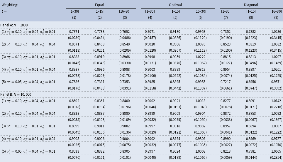
Notes: The table shows estimated persistence for various $T$
,
$T$
, $N$
, and weighting schemes from simulated data for
$N$
, and weighting schemes from simulated data for $\rho = 0.9$
and various values for the variances of fixed effects and shocks.
$\rho = 0.9$
and various values for the variances of fixed effects and shocks. $\sigma ^2_\alpha$
,
$\sigma ^2_\alpha$
, $\sigma ^2_\eta$
, and
$\sigma ^2_\eta$
, and $\sigma ^2_\epsilon$
are the variances of fixed effects, persistent, and transitory shocks, respectively. Standard errors are in parentheses.
$\sigma ^2_\epsilon$
are the variances of fixed effects, persistent, and transitory shocks, respectively. Standard errors are in parentheses.
Row (1) focuses on the benchmark parameters for the variances of fixed effects, persistent, and transitory shocks. Column (1) shows the results for estimations utilizing the first thirty periods of simulated data. There is a sizeable downward bias in the estimated persistence that equals about 0.10. Row (2) holds the variance of fixed effects and transitory shocks fixed but increases the variance of persistent shocks to 0.04. The estimated persistence is, on average, 0.867, featuring a smaller downward bias relative to that in row (1). Row (3) conducts a comparative statics exercise of lowering the variance of transitory shocks from 0.04 in row (1) to 0.01. The estimated persistence is now 0.898, so the bias nearly vanishes. Row (4) conducts a comparative statics exercise of increasing the variance of persistent shocks from 0.01 in row (3) to 0.04 while keeping the variance of transitory shocks at a low value of 0.01. The estimated persistence is somewhat higher than in row (3) but close to the true value. Summing up, it appears that increasing the variance of transitory shocks raises a downward bias in the estimated persistence, more so when the variance of persistent shocks is low. The downward bias becomes smaller with an increase in the variance of persistent shocks. Both of these effects indicate that a higher ratio of transitory to persistent variances results in a bigger downward bias in the estimated persistence. Row (5) conducts a comparative statics exercise of lowering the variance of fixed effects to 0.05 from 0.10 in row (1) and shows that the downward bias becomes bigger when the variance of fixed effects is smaller. In column (2), we use the first fifteen years of the simulated data, whereas in column (3), we use its last fifteen years. The results are qualitatively similar—with generally bigger downward biases than in column (1)—and, as expected, are less precise.
In Panel B, rows (1)–(5), we conduct the same analysis but now for samples that are ten times bigger cross-sectionally. A downward bias in the estimated persistence remains substantial when the ratio of the variance of transitory to persistent shocks is high, rows (1) and (5), but nearly vanishes for the other experiments in rows (2) to (4).
4.1.2 High persistence
Table 2 repeats the analysis of Table 1 for the persistence of long-lasting shocks equal to 0.995. The results are similar overall, although, in addition, a substantive downward bias remains even when $N=10,000$
and the variances of persistent and transitory shocks are both low, Panel B row (3).
$N=10,000$
and the variances of persistent and transitory shocks are both low, Panel B row (3).
Estimated persistence. True persistence $\rho =0.995$
. Zero initial conditions
$\rho =0.995$
. Zero initial conditions
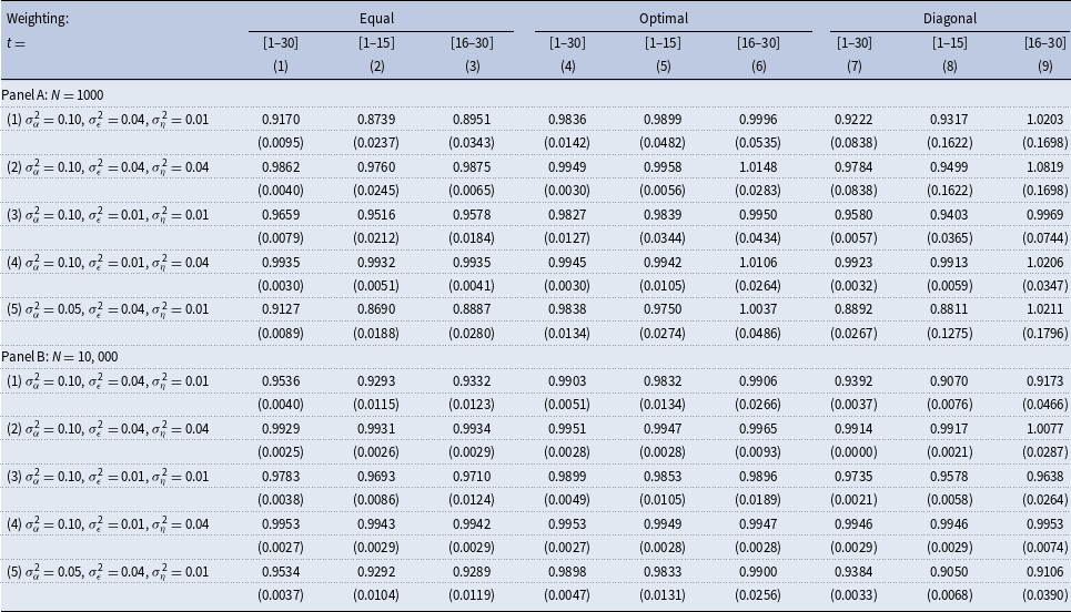
Notes: The table shows estimated persistence for various $T$
,
$T$
, $N$
, and weighting schemes from simulated data for
$N$
, and weighting schemes from simulated data for $\rho = 0.995$
and various values for the variances of fixed effects and shocks.
$\rho = 0.995$
and various values for the variances of fixed effects and shocks. $\sigma ^2_\alpha$
,
$\sigma ^2_\alpha$
, $\sigma ^2_\eta$
, and
$\sigma ^2_\eta$
, and $\sigma ^2_\epsilon$
are the variances of fixed effects, persistent, and transitory shocks, respectively. Standard errors are in parentheses.
$\sigma ^2_\epsilon$
are the variances of fixed effects, persistent, and transitory shocks, respectively. Standard errors are in parentheses.
4.2 Optimal weighting
4.2.1 Low persistence
Using an optimal weighting matrix and the first thirty periods of the simulated data produces nearly unbiased estimates of the persistence; see column (4) of Table 1. Using the first fifteen periods makes the estimates somewhat noisier, but the results are qualitatively similar. This is true both for samples with small and big $N$
, Panels A and B, respectively. Using the last fifteen periods produces a substantial upward bias in the estimated persistence. The key difference between the samples used in columns (4) and (5) versus column (6) is that, in the latter case, the variance of incomes in the first panel year is substantially higher due to the accumulation of persistent shocks. We will show below that the high variability of the persistent component in the first sample year is the driver of the divergent results for the first fifteen vs. the last fifteen periods.
$N$
, Panels A and B, respectively. Using the last fifteen periods produces a substantial upward bias in the estimated persistence. The key difference between the samples used in columns (4) and (5) versus column (6) is that, in the latter case, the variance of incomes in the first panel year is substantially higher due to the accumulation of persistent shocks. We will show below that the high variability of the persistent component in the first sample year is the driver of the divergent results for the first fifteen vs. the last fifteen periods.
4.2.2 High persistence
For the case of high persistence, using the first fifteen periods in estimation produces substantively downward-biased estimates of the persistence even if the number of sample individuals is large when the ratio of the variance of transitory to persistent shocks is large or when both persistent and transitory variances are small—rows (1) and (5), and row (3) in Table 2, respectively. Similar to the case of low persistence, optimal weighting typically produces upward-biased estimates of the persistence when the number of sample individuals is small, and one uses the last fifteen sample periods. However, the bias is small in magnitude.
4.3 Diagonal weighting
Diagonal weighting produces results similar to equal weighting when (i) the true persistence is high, and the number of individuals is large; (ii) when the true persistence is high, the number of individuals is low, and one uses the first fifteen or the first thirty sample periods; or (iii) when the true persistence is low, and one uses the first fifteen or the first thirty sample periods, regardless of the number of sample individuals. Diagonal weighting produces results similar to optimal weighting when (i) the true persistence is low, and one uses the last fifteen sample periods, or (ii) when the true persistence is high, and one uses the last fifteen sample periods when the number of sample individuals is small.
4.4 Nonzero initial conditions
In period 16, the variance of the persistent component equals $\sigma ^2_\eta (1-\rho ^{32})/(1-\rho ^2)$
when the initial variance of the persistent component is zero—see equation (2). To verify our conjecture above that it is the variance of the persistent component in the first sample year that makes our diagonal and optimal weighting results for periods
$\sigma ^2_\eta (1-\rho ^{32})/(1-\rho ^2)$
when the initial variance of the persistent component is zero—see equation (2). To verify our conjecture above that it is the variance of the persistent component in the first sample year that makes our diagonal and optimal weighting results for periods $t=1,\ldots,15$
and
$t=1,\ldots,15$
and $t=16,\ldots,30$
diverge, we conduct separate experiments where we assume that
$t=16,\ldots,30$
diverge, we conduct separate experiments where we assume that $\hbox{var}(z_{i0})=\sigma ^2_\eta (1-\rho ^{30})/(1-\rho ^2)$
. We then simulate data for fifteen periods and compare the results with those in Tables 1–2 that are based on zero initial conditions and the last fifteen periods. By design, income variances in the first sample year in these experiments are identical.Footnote
9
For convenience, columns (4)–(6) and (10)–(12) of Table 3 reproduce our results from Tables 1–2 for low and high persistence, respectively. Reassuringly, our new results in columns (1)–(3) and (7)–(9) of Table 3 based on nonzero initial conditions are nearly identical to the corresponding results in the reproduced columns, both in small and large samples. For example, using the first fifteen periods of the samples with nonzero initial conditions and diagonally weighted estimation produces a substantial upward bias in the persistence when the true persistence is low—column (3) Panels A and B of Table 3. Those results are nearly the same in all of our experiments when we use the last fifteen periods of the data with zero initial conditions and diagonally weighted estimation—column (6) of Panels A and B.
$\hbox{var}(z_{i0})=\sigma ^2_\eta (1-\rho ^{30})/(1-\rho ^2)$
. We then simulate data for fifteen periods and compare the results with those in Tables 1–2 that are based on zero initial conditions and the last fifteen periods. By design, income variances in the first sample year in these experiments are identical.Footnote
9
For convenience, columns (4)–(6) and (10)–(12) of Table 3 reproduce our results from Tables 1–2 for low and high persistence, respectively. Reassuringly, our new results in columns (1)–(3) and (7)–(9) of Table 3 based on nonzero initial conditions are nearly identical to the corresponding results in the reproduced columns, both in small and large samples. For example, using the first fifteen periods of the samples with nonzero initial conditions and diagonally weighted estimation produces a substantial upward bias in the persistence when the true persistence is low—column (3) Panels A and B of Table 3. Those results are nearly the same in all of our experiments when we use the last fifteen periods of the data with zero initial conditions and diagonally weighted estimation—column (6) of Panels A and B.
Estimated persistence. Nonzero vs. Zero initial conditions
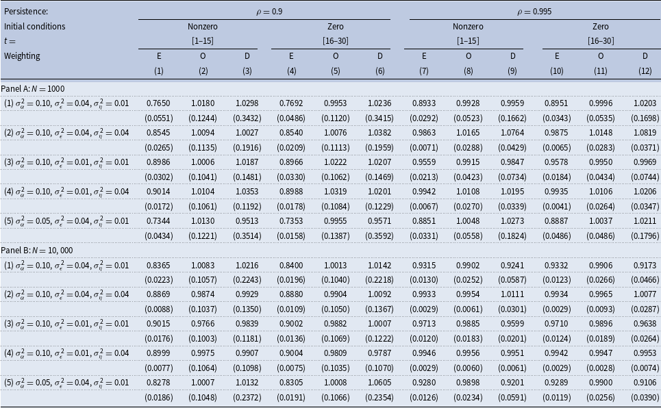
Notes: The table shows estimated persistence for various $N$
, initial conditions, and weighting schemes from simulated data for
$N$
, initial conditions, and weighting schemes from simulated data for $\rho = 0.995$
and
$\rho = 0.995$
and $\rho =0.90$
and various values for the variances of fixed effects and shocks.
$\rho =0.90$
and various values for the variances of fixed effects and shocks. $\sigma ^2_\alpha$
,
$\sigma ^2_\alpha$
, $\sigma ^2_\eta$
, and
$\sigma ^2_\eta$
, and $\sigma ^2_\epsilon$
are the variances of fixed effects, persistent, and transitory shocks, respectively. Standard errors are in parentheses. “E” [“O”] (“D”) stands for equally [optimal] (diagonally) weighted estimations. The variance of the persistent component in period 0,
$\sigma ^2_\epsilon$
are the variances of fixed effects, persistent, and transitory shocks, respectively. Standard errors are in parentheses. “E” [“O”] (“D”) stands for equally [optimal] (diagonally) weighted estimations. The variance of the persistent component in period 0, $\hbox{var}(z_{i0})$
, equals 0 or
$\hbox{var}(z_{i0})$
, equals 0 or $\sigma ^2_\eta (1-\rho ^{30})/(1-\rho ^2)$
for zero and nonzero initial conditions, respectively.
$\sigma ^2_\eta (1-\rho ^{30})/(1-\rho ^2)$
for zero and nonzero initial conditions, respectively.
An important takeaway is that even when using large samples that mix various cohorts of individuals at different stages of their life cycles, with optimal and diagonal weighting, one should expect an upward-biased estimate of persistence.
4.5 The mechanics of an upward bias in optimally- and diagonally weighted estimations
As we documented above in Tables 1–2, there is a stark difference in the estimated persistence for equal versus optimal and diagonal weighting when the true persistence is low, and one relies on the first fifteen (or first thirty periods) as opposed to the last fifteen periods. Since the number of individuals and time periods is held constant across those two scenarios, the key difference between them is the variance of persistent component in the initial period of the data—no variance of the persistent component for the samples utilizing the first fifteen periods in estimation, as we assume that initial conditions are zero for everyone, and a relatively high variance of the persistent component for the samples utilizing the last fifteen periods, due to a history of accumulation of persistent shocks.
To further explore the importance of this mechanism for the results, we simulate data for a very large number of individuals— $N=50,000$
—using our benchmark parameters and the persistence of long-lasting shocks of 0.90 and plot the minimized objective function values at each value of the persistence grid. Panels (a)–(b) of Fig. 1(A) plot the minimized objective values for the equally weighted estimations using the first fifteen and the last fifteen periods for the case of zero initial conditions, whereas Panel (c) does the same but for the estimations based on the first fifteen periods and nonzero initial conditions for the persistent component, with the variance equal to
$N=50,000$
—using our benchmark parameters and the persistence of long-lasting shocks of 0.90 and plot the minimized objective function values at each value of the persistence grid. Panels (a)–(b) of Fig. 1(A) plot the minimized objective values for the equally weighted estimations using the first fifteen and the last fifteen periods for the case of zero initial conditions, whereas Panel (c) does the same but for the estimations based on the first fifteen periods and nonzero initial conditions for the persistent component, with the variance equal to $\sigma ^2_\eta (1-\rho ^{30})/(1-\rho ^2)$
. The plots have two minima, one well below the true value of 0.90 and another one above 1 but below 1.1. All estimations capture well the global minimum that generates the downward bias in the estimated persistence we have documented in Tables 1 and 3. Panels (d)–(f) and (g)–(i) of Fig. 1(A) contain the same plots but for the optimally and diagonally weighted estimations, respectively.
$\sigma ^2_\eta (1-\rho ^{30})/(1-\rho ^2)$
. The plots have two minima, one well below the true value of 0.90 and another one above 1 but below 1.1. All estimations capture well the global minimum that generates the downward bias in the estimated persistence we have documented in Tables 1 and 3. Panels (d)–(f) and (g)–(i) of Fig. 1(A) contain the same plots but for the optimally and diagonally weighted estimations, respectively.
Objective function value at grid points for the persistence. Simulated data. Large $N$
. Notes: Each panel shows objective function values at various grid points for the persistence for equally, optimally, and diagonally weighted minimum distance estimation (EWMD, OMD, and DWMD). OMD and DWMD objective function values are divided by 1000 and 100, respectively.
$N$
. Notes: Each panel shows objective function values at various grid points for the persistence for equally, optimally, and diagonally weighted minimum distance estimation (EWMD, OMD, and DWMD). OMD and DWMD objective function values are divided by 1000 and 100, respectively.
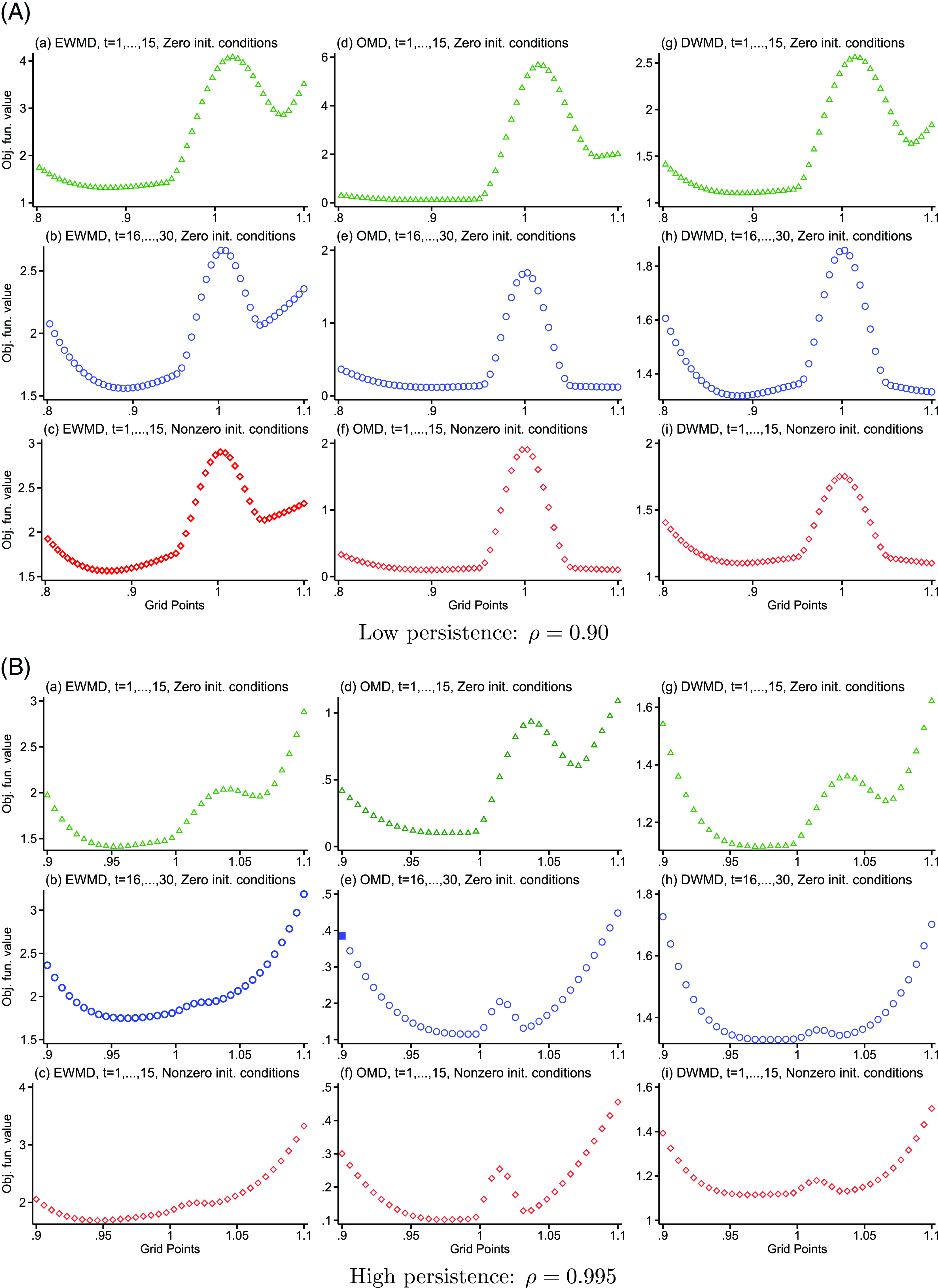
When the first fifteen periods are used in estimation, and initial conditions for the persistent component are zero, both optimal and diagonal weighting estimations capture well the global minimum visible in Panels (d) and (g). When the variance of the persistent component in the initial year of the sample is high—due to nonzero initial conditions or when using the last fifteen periods for the case of zero initial conditions—there are two local minima, one around 0.90 and another one above 1 that yield close values of the objective function; see Panels (e)–(f) for optimal and (h)–(i) for diagonal estimations, respectively. Both of these minima are frequently chosen in the estimations, resulting in an upward-biased estimate of the persistence when the variance of incomes in the first year of the sample is high and either optimally- or diagonally weighted estimations are utilized. These estimations also result in a relatively higher variability in the estimated persistence.
When the true persistence is high, equally weighted estimations using the first fifteen or the last fifteen observations produce global minima, which are well below the true value of persistence—Panels (a)–(c) of Fig. 1(B). Similar to the case of low persistence, estimations capture these global minima well. For diagonal and optimal weighting, some estimations feature local minima, below and above the true value, that are not far apart—Panels (e), (f), (h), and (i). As with the case of low persistence, these estimations result in a relatively higher variability of the estimated persistence.
5. Quantitative evaluation of the biases
In the previous section, we examined the direction of biases by varying the income process parameters one by one. In this section, we, first, compute biases in the persistence and the other parameters using the regression analysis; second, perform an empirical application of estimation in quasidifferences to Danish administrative data on male earnings; and, third, analyze biases in the income and consumption process parameters from a minimum-distance estimation based on consumption data and income data in quasidifferences from a calibrated standard incomplete markets model.
5.1 Biases in persistence
In Table 4, we report the results from regressions of a bias in the estimated persistence, $\hat{\rho }-\rho$
, on the true values for the variances of fixed effects, persistent shocks, and transitory shocks. In odd columns, we combine the samples that use the first fifteen or the first thirty observations, while in even columns, we use the simulated data for the last fifteen observations from Tables 1–2. Our analysis above emphasized that those samples yield drastically different results for the estimations relying on optimal and diagonal weighting. The dependent variable is divided by 100, and the independent variables are standardized so that they all have a mean of zero and a standard deviation of one.
$\hat{\rho }-\rho$
, on the true values for the variances of fixed effects, persistent shocks, and transitory shocks. In odd columns, we combine the samples that use the first fifteen or the first thirty observations, while in even columns, we use the simulated data for the last fifteen observations from Tables 1–2. Our analysis above emphasized that those samples yield drastically different results for the estimations relying on optimal and diagonal weighting. The dependent variable is divided by 100, and the independent variables are standardized so that they all have a mean of zero and a standard deviation of one.
Bias in the estimated persistence. Regression analysis
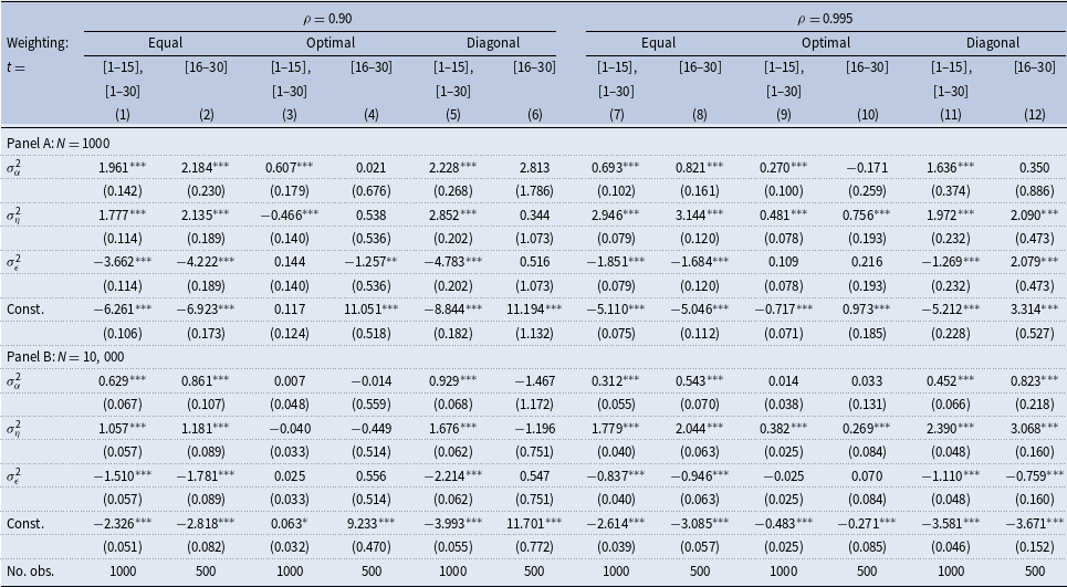
Notes: The table contains the results from a regression of the bias in the persistence scaled by 100, $100\cdot (\hat{\rho }-\rho )$
, on the standardized variances of fixed effects,
$100\cdot (\hat{\rho }-\rho )$
, on the standardized variances of fixed effects, $\sigma ^2_\alpha$
, persistent shocks,
$\sigma ^2_\alpha$
, persistent shocks, $\sigma ^2_\eta$
, and transitory shocks,
$\sigma ^2_\eta$
, and transitory shocks, $\sigma ^2_\epsilon$
. Columns
$\sigma ^2_\epsilon$
. Columns $t=$
[1–15], [1–30] (
$t=$
[1–15], [1–30] ( $t=$
[16–30]) utilize estimation data based on the first fifteen or thirty (last fifteen) observations from Tables 1–2. Standard errors are in parentheses.
$t=$
[16–30]) utilize estimation data based on the first fifteen or thirty (last fifteen) observations from Tables 1–2. Standard errors are in parentheses. $^{***}$
(
$^{***}$
( $^{**}$
) [
$^{**}$
) [ $^{*}$
] significant at the 1% (5%) [10%] level.
$^{*}$
] significant at the 1% (5%) [10%] level.
When the true persistence is low, equally weighted estimates have an average downward bias of 0.06–0.07 in small samples; the bias drops to 0.02–0.03 in samples with 10,000 individuals—see the estimated constants in columns (1)–(2) of Panel A and B, respectively. In small samples, an increase in the variance of transitory shocks by one standard deviation,Footnote
10
ceteris paribus, raises the downward bias by additional 0.04 points, resulting in an estimate of the persistence of 0.80. A reduction in the variance of persistent shocks by one standard deviation raises the downward bias by additional 0.02 points, whereas a reduction in the variance of fixed effects by one standard deviation raises the downward bias by about 0.02 points.Footnote
11
All these effects are significant at the 1% level. They are quantitatively smaller when $N$
is large, although they are still statistically significant—Panel B, columns (1)–(2). Thus, even if samples are large, a particular configuration of model parameters could result in biased estimates of the persistence.
$N$
is large, although they are still statistically significant—Panel B, columns (1)–(2). Thus, even if samples are large, a particular configuration of model parameters could result in biased estimates of the persistence.
When the true persistence is high, the average bias is similar, the effects of a variation in the variance of fixed effects and transitory shocks are somewhat smaller, whereas the effect of a change in the variance of persistent shocks is somewhat larger—columns (7)–(8).
Optimally weighted estimates have small biases when the first fifteen or thirty observations are used and little variation of these biases when the model parameters change—columns (3) and (9). An upward bias is substantial when the last fifteen observations are used, the true persistence is low, and the bias varies little with the model parameters, especially when $N$
is large—column (4).
$N$
is large—column (4).
Diagonally weighted results are quantitatively similar to the equally weighted results when the first fifteen or thirty observations are used in estimation and similar to the optimally weighted results when the last fifteen observations are used in estimation.
5.2 Biases in the other parameters
Online Appendix Tables A-1–A-3 contain the results from analogous regressions for the biases in the variance of fixed effects, persistent, and transitory shocks, respectively. Briefly, the variance of fixed effects is severely upward-biased when the true persistence is high regardless of the weighting matrix, sample size, or the number of periods. The variances of persistent and transitory shocks typically have small biases, especially when samples are large cross-sectionally. See the Online Appendix for the full details.
5.3 Empirical application
To illustrate our results empirically, we use administrative earnings records from Denmark for the cohort of males born in 1952 observed during 1981–2006. We use a balanced sample and the sample selection criteria of Daly et al. (Reference Daly, Hryshko and Manovskii2022) that are standard in the literature. Briefly, we dropped individuals who were ever self-employed, dropped records for males working less than 10% of the year as full-time employees, and earnings histories with growth outliers defined as an increase of earnings in adjacent periods by more than 500% or a drop by less than –80%. Earnings are expressed in the 1981 Danish kroner. We remove predictable variation in earnings by running, for each year, cross-sectional regressions of log earnings on educational dummies, a third-order polynomial in age, and the interaction of the educational dummies with the age polynomial. Our final sample comprises 13,543 individuals with 26 earnings observations.
As in Daly et al. (Reference Daly, Hryshko and Manovskii2022), we allow for an MA(1) transitory component but also allow for the variances of persistent and transitory shocks to vary over time.Footnote 12 Using an optimal weighting matrix and estimation in quasidifferences, similar to Daly et al. (Reference Daly, Hryshko and Manovskii2022), we find that the variance of transitory shocks is about twice as large as the variance of persistent shocks. The persistence of long-lasting shocks is estimated at 0.975, close to an estimate in Daly et al. (Reference Daly, Hryshko and Manovskii2022) for their balanced sample. Using diagonal weighting, we estimate persistence at 0.935, whereas equal weighting of the moments yields an estimate of 0.895. The most fitting reference to our empirical setting is the simulation results in rows (1) and (5) and columns (3), (6), and (9) of Table 2 Panel B. Those results are based on the experiments where the variance of transitory shocks is relatively higher than the variance of persistent shocks, samples are cross-sectionally large, and individuals have already accumulated persistent shocks for a number of years when they are first observed in the data. Similar to our empirical results, optimal weighting yields a higher estimate of the persistence than equal and diagonal weighting of the moments. Using 100 bootstrap samples of 1000 individuals from our Danish data, we obtain the average values of persistence of 0.984, 1.00, and 0.867 for optimal, diagonal, and equal weighting, respectively. This corresponds to our simulation results where the estimates of the persistence are comparable for large and small samples for optimal weighting (column (6) row (1) Panels A and B, or column (6) row (5) Panels A and B), are substantially higher in small samples when diagonal weighting is used (column (9) row (1) Panels A and B, or column (9) row (5), both panels), and are lower in small samples when equal weighting is used (column (3) row (1), or column (3) row (5) in both panels).
5.4 Biases when using consumption and income data
Blundell et al. (Reference Blundell, Pistaferri and Preston2008) developed a methodology for estimating the income process and consumption insurance parameters using auto- and cross-covariances of consumption and income growth rates. They applied it to longitudinal data from the U.S., assuming that the autoregressive component of income is a random walk. Specifically, they estimated the variances of permanent and transitory income shocks in equation (1) along with the transmission of those shocks to household consumption, evaluating the following equation:
 \begin{equation*} \Delta c_{it}=\phi \eta _{it}+\psi \epsilon _{it}+\zeta _{it}+\Delta u_{it}, \end{equation*}
where $c_{it}$
is the household
$c_{it}$
is the household $i$
’s log consumption at time
$i$
’s log consumption at time $t$
,
$t$
, $\phi$
, and
$\phi$
, and $\psi$
are the transmission coefficients for permanent and transitory income shocks to household consumption, respectively,
$\psi$
are the transmission coefficients for permanent and transitory income shocks to household consumption, respectively, $u_{it}$
is the measurement error in consumption, and
$u_{it}$
is the measurement error in consumption, and $\zeta _{it}$
is a permanent shock to consumption that is orthogonal to the income shocks.
$\zeta _{it}$
is a permanent shock to consumption that is orthogonal to the income shocks.
Estimation using quasidifferencing can be easily embedded into the methodology of Blundell et al. (Reference Blundell, Pistaferri and Preston2008) when the long-lasting component is, instead, an autoregressive process with finite persistence.Footnote 13 Although we showed above that estimation in quasidifferences is often unreliable when using income data, consumption data could provide valuable information for identifying the persistence of the shocks and, used jointly with income, might potentially help correct the biases outlined above. To explore this possibility, we simulate data from a calibration of the standard incomplete-markets model of consumption.
In the model, households value consumption, $C$
, using CRRA utility function
$C$
, using CRRA utility function $u(C)=\frac{C^{1-\gamma }}{1-\gamma }$
, face zero borrowing constraints, and accumulate savings for retirement and precautionary reasons to insulate their consumption from persistent and transitory shocks to income and the predictable income drop at retirement. The real interest rate on saving is set to 4%. Households discount future utility exponentially using the time discount factor
$u(C)=\frac{C^{1-\gamma }}{1-\gamma }$
, face zero borrowing constraints, and accumulate savings for retirement and precautionary reasons to insulate their consumption from persistent and transitory shocks to income and the predictable income drop at retirement. The real interest rate on saving is set to 4%. Households discount future utility exponentially using the time discount factor $\beta$
and face mortality risk after retirement. They start their working life at age 26, retire at age 65, and die with certainty at age 90. Income is exogenous and is subject to the persistent and transitory risk before retirement, as in equation (1). After retirement, income equals 70% of its autoregressive component at age 65.
$\beta$
and face mortality risk after retirement. They start their working life at age 26, retire at age 65, and die with certainty at age 90. Income is exogenous and is subject to the persistent and transitory risk before retirement, as in equation (1). After retirement, income equals 70% of its autoregressive component at age 65.
We focus on the two persistence values as we have done above. Those values were found to characterize the income dynamics of the families formed by sons and daughters of the original PSID households; see Hryshko and Manovskii (Reference Hryshko and Manovskii2022). The variance of persistent and transitory shocks and the variance of fixed effects are set to the benchmark values of row (1) in Table 1. We assume that all households start with zero persistent component of incomes at age 26, and all shocks and fixed effects are normally distributed. The predictable components of income and mortality risk are taken from Hryshko and Manovskii (Reference Hryshko and Manovskii2022). The time discount factor is calibrated by matching the wealth-to-income ratio in each economy characterized by different persistence of long-lasting income shocks to the value of 3. The calibrated values are 0.9529 and 0.9555 in the economies with the persistence of long-lasting shocks equal to 0.995 and 0.90, respectively. Table 5 summarizes details of the calibration.
Calibration
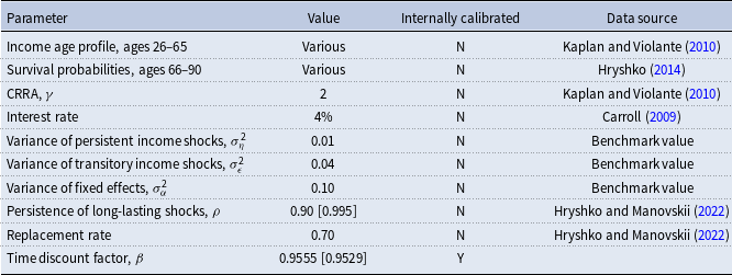
Notes: The table shows various inputs for calibrating the standard incomplete-markets economy with zero borrowing constraints. The time discount factor is calibrated internally by matching the wealth-to-income ratio in the economies characterized by different values of the persistence of long-lasting shocks to the value of 3.
We next simulate income and consumption data for a large number of households and randomly select either 1000 or 10,000 out of the simulated dataset. We assume that consumption is measured with error in the data and set the variance of measurement error to 0.04. We replicate the PSID design of the data in Hryshko and Manovskii (Reference Hryshko and Manovskii2022) by creating fifteen years of data on consumption and income and matching the age distribution in the PSID during the 1978–1992 period analyzed in Blundell et al. (Reference Blundell, Pistaferri and Preston2008) and Hryshko and Manovskii (Reference Hryshko and Manovskii2022). Specifically, we observe the distribution of birth years for households formed by sons and daughters of the original PSID households, and we use the income and consumption data when those households were 30–65 years of age within the 1978–1992 period. This is a different data structure relative to the ones we analyzed above due to the presence of various birth-year cohorts in each year. In the simulated data, similar to the PSID, households are on average 36.5 years of age in 1978 (the first year of the simulated dataset) and 42.5 years of age in 1992 (the last year of the dataset). Since many households have accumulated a substantial history of shocks prior to the first year in the simulated data, we expect our results to resemble the above results for the estimations relying on periods 16–30 of the simulated income data.
Table 6 presents the results from estimations in quasidifferences using simulated income data only and verifies this conjecture. Both for small and large samples, equal weighting yields substantial downward biases in the estimated persistence when the true persistence is low or high. Diagonal and optimal weighting yield substantial upward biases when the true persistence is low for small and large samples and some downward biases when the true persistence is high and samples are large. The estimated variances of persistent and transitory shocks are not very far from their true values, whereas the variance of fixed effects is biased, more so for the estimations on the data with high true persistence.
Estimates of the income process parameters. Data from a calibrated lifecycle model
Notes: The table shows results from estimations in quasidifferences using simulated income data from the calibrated standard incomplete-markets model for different values of persistence, $N$
, and weighting schemes. See Section 5.4 for the details on the model and simulations. Age distribution in the simulated data is as in the PSID. True values for the variance of fixed effects, persistent, and transitory shocks are 0.10, 0.01, and 0.04, respectively. Standard errors are in parentheses.
$N$
, and weighting schemes. See Section 5.4 for the details on the model and simulations. Age distribution in the simulated data is as in the PSID. True values for the variance of fixed effects, persistent, and transitory shocks are 0.10, 0.01, and 0.04, respectively. Standard errors are in parentheses.
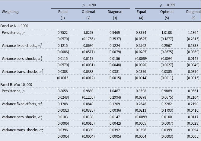
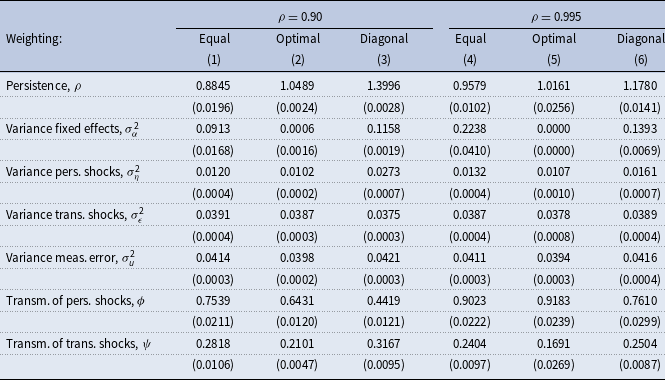
Tables 7 and 8 show the results for the income process and consumption insurance parameters from estimations using consumption data and incomes in quasidifferences in small and large samples, respectively. Equal weighting yields an estimate of persistence close to its true value when the true persistence is low and the sample is large, whereas optimal weighting yields slightly upward-biased estimates of the persistence when the true persistence is high, both in small and large samples. The variance of persistent shocks is substantially overestimated when the diagonal weighting matrix is used. The true transmission coefficients for persistent and transitory shocks in our low-persistence economy are 0.59 and 0.25, respectively. Both transmission coefficients are close to their true values when optimal weighting is used, both for small and large samples. However, in this setting, one would conclude that consumers are excessively insured against persistent income shocks since the estimated persistence is well above the true value of 0.90. Diagonal weighting produces noisy and biased estimates of the persistence and the transmission coefficient for persistent shocks in small samples and is very unreliable in large samples.
Estimates of income and consumption insurance parameters. Data from a calibrated lifecycle model, $N = 1000$
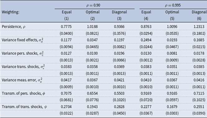
Notes: The table shows results from estimations using simulated consumption data and income data in quasidifferences from the calibrated standard incomplete-markets model for different values of persistence, $N$
, and weighting schemes. See Section 5.4 for the details on the model and simulations. Age distribution in the simulated data is as in the PSID. True values for the variance of fixed effects, persistent, and transitory shocks are 0.10, 0.01, and 0.04, respectively. Standard errors are in parentheses.
$N$
, and weighting schemes. See Section 5.4 for the details on the model and simulations. Age distribution in the simulated data is as in the PSID. True values for the variance of fixed effects, persistent, and transitory shocks are 0.10, 0.01, and 0.04, respectively. Standard errors are in parentheses.
Estimates of income and consumption insurance parameters. Data from a calibrated lifecycle model, $N= 10,000$
Notes: The table shows results from estimations using simulated consumption data and income data in quasidifferences from the calibrated standard incomplete-markets model for different values of persistence, $N$
, and weighting schemes. See Section 5.4 for the details on the model and simulations. Age distribution in the simulated data is as in the PSID. True values for the variance of fixed effects, persistent, and transitory shocks are 0.10, 0.01, and 0.04, respectively. Standard errors are in parentheses.
$N$
, and weighting schemes. See Section 5.4 for the details on the model and simulations. Age distribution in the simulated data is as in the PSID. True values for the variance of fixed effects, persistent, and transitory shocks are 0.10, 0.01, and 0.04, respectively. Standard errors are in parentheses.
The true transmission coefficients for persistent and transitory shocks in our high persistence economy are 0.90 and 0.20, respectively. Diagonal weighting substantially underestimates the transmission of persistent shocks to consumption. Equal weighting yields transmission coefficients that are close to their true values in small and large samples yet significantly underestimates the persistence, producing an erroneous impression of underinsurance of persistent income shocks. Diagonal weighting produces slightly biased transmission coefficients but an upward-biased estimate of the variance of persistent shocks.
To sum up, using data from a calibrated lifecycle model of consumption, we showed, for the benchmark income parameters, that the estimated income and consumption process parameters are biased regardless of the weighting scheme and the number of sample households.
6. Implications
Despite its virtues in implementation, estimation in quasidifferences is biased in the predominant number of cases we considered. What are the implications for researchers who wish to rely on quasidifferences to recover the income process parameters? There are a number of positive results from our analysis. First, looking closely at the results in Tables 1–3 reveals that, regardless of the sample size, initial conditions, or the true persistence, the estimated persistence is virtually unbiased if one uses equally weighted estimation when the variance of persistent shocks is significantly bigger than the variance of transitory shocks—columns (1)–(3) and row (4) of Tables 1 and 2, and columns (1) and (7), row (3) in Table 3.Footnote 14 Although this is not characteristic of U.S. survey and administrative data,Footnote 15 it is the case for administrative income data from Norway as was found in Blundell et al. (Reference Blundell, Graber and Mogstad2015). This result is based on the knowledge of the relative variances of persistent and transitory shocks, not available a priori. However, our second positive result is that the variances of persistent and transitory shocks are not significantly biased for the cases we considered. Our advice, therefore, is to apply an equally weighted estimation of the income process in quasidifferences and use the results with confidence if the variance of persistent shocks is found to be larger than the variance of transitory shocks. It would be ideal to have a robust method for correcting the biases in all other circumstances, but unfortunately, after some experimentation, we could not come up with such a method.Footnote 16
7. Conclusion
The income process parameters are key in quantitative models featuring incomplete insurance markets. To recover the parameters, one typically matches autocovariance moments for incomes in levels or growth rates. Blundell et al. (Reference Blundell, Graber and Mogstad2015) recently applied estimation in quasidifferences to administrative data on incomes from Norway, assuming a variant of the canonical income process featuring fixed effects, persistent, and transitory components. Estimation in quasidifferences combines the features of estimations in levels and differences but relies on more concise moments when the true persistence of long-lasting shocks is different from one. It also requires searching through a predefined grid for the persistence of autoregressive shocks, as the persistence is not jointly identified with the other parameters. In contrast to a voluminous GMM literature, nothing is known about how well the persistence is recovered using estimation in quasidifferences. In this paper, we provide a guide to estimating the canonical income process using quasidifferences by conducting Monte Carlo simulations and cataloging biases for various $N$
,
$N$
, $T$
, initial conditions, and weighting schemes. We find that equally weighted estimations result in downward-biased estimates of the persistence when the variance of transitory shocks is higher than the variance of persistent shocks, whereas optimally and diagonally weighted estimations result in upward-biased estimates of the persistence when the variance of the persistent component in the first sample year is nonnegligible, which is a typical feature of the data containing individuals of different ages in the first sample year of the data. The variance of fixed effects is substantially biased upward when the true persistence is high. The biases in the estimated variances of persistent and transitory shocks are, however, small. Our estimations based on Danish administrative earnings data yield divergent estimates of the persistence for different weighting schemes, which conform to the simulated results for the high persistence and nonzero initial conditions. Using data from a calibrated lifecycle model of consumption, we also show, for the benchmark income parameters, that the estimated income and consumption process parameters are biased regardless of the weighting scheme and the number of sample households.
$T$
, initial conditions, and weighting schemes. We find that equally weighted estimations result in downward-biased estimates of the persistence when the variance of transitory shocks is higher than the variance of persistent shocks, whereas optimally and diagonally weighted estimations result in upward-biased estimates of the persistence when the variance of the persistent component in the first sample year is nonnegligible, which is a typical feature of the data containing individuals of different ages in the first sample year of the data. The variance of fixed effects is substantially biased upward when the true persistence is high. The biases in the estimated variances of persistent and transitory shocks are, however, small. Our estimations based on Danish administrative earnings data yield divergent estimates of the persistence for different weighting schemes, which conform to the simulated results for the high persistence and nonzero initial conditions. Using data from a calibrated lifecycle model of consumption, we also show, for the benchmark income parameters, that the estimated income and consumption process parameters are biased regardless of the weighting scheme and the number of sample households.
The results in our paper provide a warning against the routine use of estimation in quasidifferences despite its attractive features. However, there is one case when estimation in quasidifferences recovers the true persistence of long-lasting shocks. When the variance of persistent shocks is higher than the variance of transitory shocks, equally weighted estimation is reliable for different $T$
,
$T$
, $N$
, and initial conditions. Since biases in the variances of the shocks using estimation in quasidifferencs are small, our advice is to estimate the income process using equal weighting of the moments and use the results with confidence if the estimated variance of persistent shocks is higher than the variance of transitory shocks. This is, for example, the case for Norwegian administrative data as shown in Blundell et al. (Reference Blundell, Graber and Mogstad2015).
$N$
, and initial conditions. Since biases in the variances of the shocks using estimation in quasidifferencs are small, our advice is to estimate the income process using equal weighting of the moments and use the results with confidence if the estimated variance of persistent shocks is higher than the variance of transitory shocks. This is, for example, the case for Norwegian administrative data as shown in Blundell et al. (Reference Blundell, Graber and Mogstad2015).
Supplementary material
The supplementary material for this article can be found at https://doi.org/10.1017/S1365100523000457


 Open access