

1. INTRODUCTION
The application of geophysical techniques in glaciology provides useful insights into the physics of glaciers (Petrenko and Whitworth, Reference Petrenko and Whitworth2002) and a valuable contribution to the study of the evolution of the climate in the past, as well as the overall impact of present climate change on the terrestrial cryosphere (Seppi and others, Reference Seppi2015). The active seismic and radio-echo sounding (RES) methods are the most popular and widely used geophysical imaging techniques in determining glacier properties (Christianson and others, Reference Christianson, Jacobel, Horgan, Anandakrishnan and Alley2012; Horgan and others, Reference Horgan2012; Carturan and others, Reference Carturan2013), while the application of geoelectric methods is still very limited (Bentley, Reference Bentley1977; De Pascale and others, Reference De Pascale, Pollard and Williams2008) and mostly orientated towards the study of permafrost (Pant and Reynolds, Reference Pant and Reynolds2000; Hilbich and others, Reference Hilbich, Marescot, Hauck, Loke and Mäusbacher2009). Besides enabling the calculation of glacier thickness and ice mass balance, these methods can provide useful information on the physical properties of the ice (e.g. Matsuoka and others, Reference Matsuoka2003; Picotti and others, Reference Picotti, Vuan, Carcione, Horgan and Anandakrishnan2015) and the subglacial environments (e.g. Blankenship and others, Reference Blankenship, Bentley, Rooney and Alley1986; Zirizzotti and others, Reference Zirizzotti, Cafarelli and Urbini2012). In any case, these methods require considerable economic and operational efforts and can be used only where the logistic difficulties are easily overcome.
On the other hand, passive seismic methods are typically applied to icequake location and characterization (e.g. Jones and others, Reference Jones, Kulessa, Doyle, Dow and Hubbard2013). These observations, however, could provide useful information on the physical properties of ice and bedrock. Anandakrishnan and Bentley (Reference Anandakrishnan and Bentley1993) used microtremor measurements to provide evidence for highly deformable till and water layers located beneath two fast flowing ice streams in West Antarctica. In a recent work, Diez and others (Reference Diez2016) estimated the S-wave velocity structure of the Ross Ice Shelf in West Antarctica, by inverting the surface-wave dispersion curves from ambient noise measurements. A similar approach has been adopted by Picotti and others (Reference Picotti, Vuan, Carcione, Horgan and Anandakrishnan2015) to determine the firn and ice S-wave velocity structure of a West Antarctic ice stream, where in this case the surface (Rayleigh and Love) waves were artificially generated.
Passive seismic can help to mitigate the logistic problems inherent in the geophysical imaging methods, by using portable broadband seismometers and the horizontal-to-vertical component spectral ratio (HVSR) technique. The great advantage of this approach, in addition to the reduced size and weight of passive seismic equipment, is that there is no need to generate elastic waves artificially. In fact, seismic noise measurements do not require the use of active seismic sources such as guns, vibrators or explosives detonated in boreholes.
The aim of this work is to verify the reliability of the HVSR technique in determining glacier thicknesses and basal properties from ambient seismic noise observations. Microtremor measurements and the HVSR technique are generally used for site-effect studies, related to the amplification mechanisms of seismic waves in shallow geological layers (e.g. Bonnefoy-Claudet and others, Reference Bonnefoy-Claudet2006, and references therein), as well as to determine the thickness of soft sediment layers (e.g. Bard and Bouchon, Reference Bard and Bouchon1985; Barnaba and others, Reference Barnaba2010). The HVSR method, originally introduced by Nogoshi and Igarashi (Reference Nogoshi and Igarashi1971) and first applied by Nakamura (Reference Nakamura1989), is based on the frequency spectra obtained by dividing the horizontal component by the vertical component of the recorded wavefield, hereafter referred to as the H/V spectra. Under some assumptions about the underground structure, it is commonly acknowledged that the HVSR method reveals the fundamental resonance frequency of a site (e.g. Lachet and Bard, Reference Lachet and Bard1994; Ibs-von Seht and Wohlenberg, Reference Ibs-von Seht and Wohlemberg1999). The first significant and detailed theoretical tests of the method were performed by Lachet and Bard (Reference Lachet and Bard1994). Using numerical simulations of ambient noise in a soil layer lying over a hard bedrock, they showed that the peak of the H/V spectral ratio is mainly related to the fundamental-mode Rayleigh wave and is very close to the body S-wave resonant frequency of the layer. A similar result is found for the H/V ratio obtained for incident plane SV-waves. Konno and Ohmachi (Reference Konno and Ohmachi1998) further improved the theory by formulating the HVSR technique in terms of the characteristics of both Rayleigh and Love waves, and introduced a simple formula for the S-wave amplification factor expressed in terms of the H/V ratio. They stated that the H/V spectra provide a reliable estimate of the fundamental resonant frequency for a site only under the condition that a sufficiently high S-wave impedance contrast between soft sediments and bedrock is present. Furthermore, Konno and Ohmachi (Reference Konno and Ohmachi1998) recommended to use not only the peaks but also the troughs in the H/V spectra, as an additional control on the natural frequency of a layer. It is now commonly accepted that surface waves play an important role in the application of the HVSR technique. Arai and Tokimatsu (Reference Arai and Tokimatsu2004) proposed that the shape and the amplitude of the H/V spectra are mainly controlled by the variations of the Rayleigh wave ellipticity (the ratio of the horizontal axis to the vertical axis of the ellipse described by the particle motion of Rayleigh waves) and by the content of Love waves in the ambient noise wavefield, respectively. Moreover, they proposed a formulation for the HVSR forward modeling where both Rayleigh and Love waves are included. Several viscoelastic numerical tests of the method have been carried out in the frame of the SESAME European Project, whose results can mainly be found in Bonnefoy-Claudet and others (Reference Bonnefoy-Claudet2006, Reference Bonnefoy-Claudet, Köhler, Cornou, Wathelet and Bard2008). These studies showed how the H/V spectral peaks generally correspond to a superposition of Rayleigh-wave, Love-wave and/or body S-wave resonances. Nevertheless, the H/V spectral ratio provides a reliable estimate of the body S-wave transfer (or amplification) function at the site, i.e., the ratio of displacement amplitudes between the top and bottom of the soil layer. In a recent study Carcione and others (Reference Carcione, Picotti, Francese, Giorgi and Pettenati2017) studied the effect of viscoelasticity on the S-wave amplification function and verified that attenuation and bedrock deformability affect the resonance peaks, with the latter having a stronger effect.
A recent interesting approach to the interpretation of the H/V spectra of microtremors is the concept of diffuse fields in layered media (e.g. Kawase and others, Reference Kawase, Matsushima, Satoh and Sánchez-Sesma2015). This theory is based on the assumption that the energy of a wavefield, produced by multiple scattering of randomly applied point sources on the surface, is equipartitioned among P- and body S-waves and Love and Rayleigh waves.
To our knowledge, the HVSR method has never been applied on ice, with the purpose of determining glacier thicknesses and basal properties. We report here the results of some experiments on the reliability of this technique, successfully applied to five glaciers of the Alpine chain. As an additional example, we show the application of the method on a West Antarctic ice stream. The HVSR results were validated using RES (also known as Ground Penetrating Radar – GPR), geoelectrical and active seismic profiling methods.
2. THE HVSR METHODOLOGY
2.1. Theory overview
The HVSR method is based on the frequency H/V spectrum obtained by dividing the horizontal component by the vertical component. Either displacement, particle velocity or acceleration can be used in the spectrum computation, since the results are equivalent. The source can be ambient noise, earthquakes or active sources of a different nature, for example, explosives or vibroseis. It has been shown that for Rayleigh waves propagating in a layer over a half space, the method yields the fundamental S-wave resonance frequency and the related amplitude (Lermo and Chávez García, Reference Lermo and Chávez García1993). In general, the 2-D resonance is caused by the trapping of seismic waves in soft layered media overlying a solid bedrock, and the spectral peaks correspond to a superposition of Rayleigh-wave, Love-wave and/or body S-wave resonance modes (Bonnefoy-Claudet and others, Reference Bonnefoy-Claudet, Köhler, Cornou, Wathelet and Bard2008). Bard and Bouchon (Reference Bard and Bouchon1985) investigated the response of sediment-filled valleys to incoming plane SH, SV and P waves, showing that nonplanar interfaces cause the generation of surface waves at the valley edges, which remain trapped within the sediments. An incident SH wave results in the generation of Love waves, while incident SV or P waves generate Rayleigh surface waves. In both cases, when the wavelengths of the incident wave are comparable with the thickness of the sedimentary layer, resonance occurs and the resulting surface waves may have much larger amplitude than the direct incident signal. Using numerical simulations of wave propagation in a soil layer lying over a rigid bedrock, Lachet and Bard (Reference Lachet and Bard1994) showed that there is a good agreement between the H/V peak positions derived for ambient noise and those obtained for SV waves. This shows that the H/V ratio gives a reliable indication of the S-wave resonance frequency of a horizontally layered structure, notwithstanding that the shape of the H/V spectra is primarily determined by the fundamental-mode Rayleigh waves.
Let us consider a hardrock basement covered by a soft layer composed by sediments or, as in our case, by ice. This waveguide structure, very effective in trapping the energy carried by elastic waves, is typical of a glacier. Ignoring wave attenuation and bedrock deformability (lossless-rigid approximation) the fundamental (body) S-wave resonance frequencies corresponding to a 2-D basin of half-width w and thickness h are
 $$f_{SH} = f_0 \sqrt {1 + (h/w)^2} $$
 $$f_{SV} = f_0 \sqrt {1 + 2.9(h/w)^2}, $$
(Bard and Bouchon, Reference Bard and Bouchon1985), where f 0 = v S/4h and v S is the low-frequency S-wave velocity. The half-width w is defined as the length over which the local soft layer thickness is greater than half the maximum thickness. If the horizontal extent of the basin is much larger than the layer thickness, we are in the 1-D approximation and the equations simplify as follows: f SH = f SV = f 0. In case of several soft layers over bedrock, the S-wave velocity is averaged using the time-average equation. A particular case consists of an extensive 2-D basin (1-D approximation), where the medium is laterally homogeneous and the seismic velocity continuously increases with depth, reaching its maximum value at depth h. Representing this S-wave vertical velocity profile by a generalized nonlinear gradient v S(z), the corresponding fundamental resonant frequency f 0 can be computed as
 $$f_0 = \displaystyle{1 \over {4T_0}}, \;\;T_0 = \int_0^h \displaystyle{{dz} \over {v_{\rm S} (z)}},$$
(Ibs-von Seht and Wohlenberg, Reference Ibs-von Seht and Wohlemberg1999), where T 0 is the S-wave traveltime along a vertical path between the bottom of the layer and the surface.
The H/V spectra may exhibit not only a peak at frequency f 0, but also a trough (minimum) at a higher frequency f 1. Konno and Ohmachi (Reference Konno and Ohmachi1998) found that H/V spectra tend to show the peak/trough structure when a site has soft surface soils and they investigated the variability of the ratio f 1/f 0 reporting a value of ~2. Recent studies (e.g. Tuan and others, Reference Tuan, Scherbaum and Malischewsky2011) concluded that the peak/trough structure indicates a high Poisson ratio in the surface soil, and a high impedance contrast at the underlying bedrock interface. If either or both these two values are high, there is a transition of the particle orbit from retrograde to prograde at a certain frequency range. The troughs correspond to the vanishing of the horizontal components, and to a reverse rotation direction, which causes a change of the ellipticity ratio of the fundamental mode.
Intrinsic attenuation and bedrock deformability affect the amplitude and frequency of the resonance peaks. Carcione and others (Reference Carcione, Picotti, Francese, Giorgi and Pettenati2017) studied the effects of anelasticity on the S-wave amplification function and found that while attenuation (quantified by the Q factor) controls the damping of the higher modes, it does not affect significantly the peak locations. On the other hand, the impedance contrast α between the layer and the bedrock strongly affects the resonance frequencies. In particular, when α ≤ 1 (soft over stiff medium) the first maximum of the S-wave amplification function is located at the fundamental frequency f 0. Conversely, α ≥ 1 (stiff over soft medium) gives a minimum at f 0 and the first maximum is located at f 1 = 2f 0. Therefore, bedrock elasticity (i.e. deformation) must be considered to obtain reliable estimations of the layer thickness.
2.2. H/V spectra computation
In the present work, the H/V spectra are obtained using the free software GEOPSY (http://www.geopsy.org – SESAME Project). The software performs a statistical analysis of the recorded wavefield in the frequency domain, by computing the amplitude spectra of the three components in a number of selectable time windows. The width of these windows depends on the target frequency band and on the record length. For the computation of the H/V ratio, the amplitude spectra of the horizontal components are combined using vector summation. An anti-triggering algorithm (Withers and others, Reference Withers1998) was applied to the time series in order to include in the computation only signals with quasi-stationary amplitudes. For all the considered cases the time windows can overlap by 5%. The selection criteria are based on the comparison between the short term (STA) and long term (LTA) average amplitudes. The algorithm selects only the parts of the signal for which the STA/LTA ratio stays within a limited range of values ~1. The upper bound of this ratio aims at excluding spikes produced for example by operators walking close to the sensors. The typical values for STA, LTA, minimum STA/LTA and maximum STA/LTA are 1, 30, 0.2 and 2.5 s, respectively. A smoothing function has been applied in the frequency analysis (Konno and Ohmachi, Reference Konno and Ohmachi1998) to ensure a constant number of points at low and high frequencies. In this work we applied a smoothing function with a cosine taper of 5% width and a smoothing constant of 25.
2.3. Rayleigh-wave ellipticity inversion
In 1-D structures, if the shape of the H/V spectra is primarily controlled by the propagation of Rayleigh waves, the P- and S-wave vertical velocity profiles of the subsurface can be determined by inverting the ellipticity of the fundamental-mode Rayleigh wave. GEOPSY includes a package (Dinver) for ellipticity inversion, based on the continuous wavelet transform (Fäh and others, Reference Fäh, Kind and Giardini2001). The mother wavelet used in the transform is defined as the Morlet wavelet, consisting in a complex exponential modulated by a Gaussian envelope (Goupillaud and others, Reference Goupillaud, Grossman and Morlet1984). This wavelet is characterized by a well-defined central frequency and allows for the extraction of phase information. The algorithm performs a time-frequency analysis on each of the three components of ambient vibrations to reconstruct the P-SV particle motion. To this aim, it is necessary to compensate for the energy of body and Love waves present in the ambient vibration recordings. This correction is done by assuming that, in laterally homogeneous structures, the vertical component close to the H/V fundamental peak is dominated by Rayleigh waves, and that the SH propagation phenomena (both body and surface waves) contribute only to the horizontal component of motion. Under this condition, and other assumptions concerning the spectral content of SH-waves (e.g. Fäh and others, Reference Fäh, Kind and Giardini2001), the algorithm tries to minimize the SH-wave content by identifying the P-SV wavelets along the signal and by computing the spectral ratio from these wavelets only. Since the method does not separate the contributions of the different modes, it is necessary to manually select the most energetic peak on the H/V spectrogram. However, the above assumptions and the condition of strongly excited fundamental-mode Rayleigh waves are often incorrect (e.g. presence of energetic higher modes). For this reason, this ellipticity-based method applies only to sites presenting a strong S-wave impedance contrast between the uppermost layer and the underlying bedrock.
Dinver is a general environment for ellipticity and surface-wave dispersion curves inversion based on a hybrid Monte Carlo optimization scheme. Currently it implements a modified version of the neighborhood algorithm (Wathelet, Reference Wathelet2008) to drive the inversion to converge to a minimum misfit solution. For each generated model, the algorithm computes the misfit between the theoretical fundamental-mode Rayleigh wave ellipticity and the ellipticity curve obtained from the time-frequency analysis of the H/V spectrograms (Wathelet and others, Reference Wathelet, Jongmans and Ohrnberger2004). The models consist of horizontal and homogeneous flat layers, in which the P- and S-wave velocity, Poisson ratio and density values are defined. Because of the multi-parametric and nonlinear character of the ellipticity inversion problem, to obtain reliable models it is convenient to constrain the parameters defined in each layer by using information from other geophysical or geological investigations.
The ellipticity inversion technique is only valid for a relatively minor influence of Love and body waves on the recorded wavefield. In other words, it is feasible only if the H/V spectrum is representative of the fundamental-mode Rayleigh wave ellipticity. If this condition is not satisfied, the velocity profiles obtained by inverting ellipticity can be quite different than the real profiles. This approach has been applied to deep sedimentary basins and for shallow sites (e.g. Fäh and others, Reference Fäh, Kind and Giardini2001) but, to our knowledge, it has never been used in glacial environments.
3. CASE STUDIES
In order to verify the reliability of the HVSR technique in different glacier settings we selected the following five target Alpine chain glaciers (Fig. 1): the Pian di Neve and Lobbia glaciers in the Adamello massif (Italy), the Forni and La Mare glaciers in the Ortles-Cevedale massif (Italy) and the Aletschgletscher in the Bernese Oberland Alps (Switzerland). We also analyzed passive seismic data previously acquired on the Whillans Ice Stream (WIS), a fast flowing ice stream in West Antarctica (see details in Horgan and others, Reference Horgan2012; Picotti and others, Reference Picotti, Vuan, Carcione, Horgan and Anandakrishnan2015).
Location of the five study sites in the Alpine chain (upper central panel); survey map of Aletsch glacier (a), Forni glacier (b), La Mare glacier (c) and Pian di Neve and Lobbia glaciers (d).The survey locations are listed in Table 1.

Four geophysical methodologies have been employed in this work, i.e., RES, geoelectric, active multichannel and passive seismic methods. Several exploration campaigns were conducted on the five target glaciers between April 2013 and October 2015 (Fig. 1 and Tables 1 and 2). In August 2013, October 2013, 2014 and 2015, passive and active seismic data were acquired on the Pian di Neve and Lobbia glaciers (Fig. 1d). In November 2013, passive seismic measurements and two mutually orthogonal RES surveys were conducted on the Forni glacier (Fig. 1b). In order to test the reliability of the HVSR method on deep and shallow glaciers, RES surveys and passive seismic measurements on the Aletsch glacier (April 2013 and May 2014; Fig. 1a) and on the La Mare glacier (April 2015 and May 2015; Fig. 1c) were carried out. The passive seismic measurements were conducted using different broadband seismometers, a Guralp, a Lennartz and a Nanometrics Trillium, whose corner periods are 30, 5 and 20 s, respectively. We also tested a Tromino sensor, whose corner period is not declared by the manufacturer. The Guralp and Lennartz sensors were connected to a Reftek data acquisition system, while the Trillium sensor was coupled to a Centaur data system. The two systems include an external GPS for positioning and timing purposes. In order to optimize the coupling, the sensors were protected using insulating covers and placed on a plexiglas or metal base directly in contact (when possible) with the ice, at the bottom of deep holes dug or excavated right into the snow and firn. The hole depth ranged from half a meter to ~4 m depending on the snow coverage. This particular coupling greatly improved data quality, by reducing the noise generated by the wind and by protecting the sensor from the sun, which can lead to thermal drifts. The sensors were always oriented parallel to the ice flow direction.
Data characteristics and computed thicknesses

* Locations A3, P1 and LM3 (see Fig. 1) are omitted because these surveys provided poor data.
† Used in the statistical analysis for the H/V spectra computation.
‡ Average resonance frequency related to firn.
Glacier thicknesses

* Outside Konkordiaplatz.
† Inside Konkordiaplatz.
‡ Firn thickness.
Data acquisition details and results obtained at each study site are described below, while the analytical techniques adopted for the geophysical imaging methods (i.e. RES, geoelectric and active seismic methods) are described in the Appendix. Tables 1 and 2 summarize the results and the main characteristics of the data collected at each site using the passive seismic method and the geophysical imaging techniques, respectively.
3.1. Pian di Neve glacier
3.1.1. The study site
The Pian di Neve is a high altitude glacier in the Adamello massif (Fig. 1d). It occupies an 8 km2 plateau at an altitude between 3100 and 3400 m a.s.l. among the main summits of the Lombardy side, i.e., the Adamello, Corno Bianco and Monte Fumo summits. Together with the adjacent Mandrone glacier, it is the largest glacier in the Italian Alps. The Pian di Neve glacier was previously investigated by Carabelli (Reference Carabelli1962) using a single-fold seismic survey (i.e. there is a single recorded trace per sub-surface point).
3.1.2. Data acquisition
Active multichannel (P and S) seismic data were acquired on the Pian di Neve glacier (Fig. 1d). Two types of active seismic surveys were undertaken using a Geometrics GEODE system: the first was devoted to assessing the firn properties while the second mostly focused on the imaging of the glacier in depth. Moreover, real-time kinematic GPS measurements were conducted to define the topography, using geodetic receivers. A shallow refraction survey, using both P and S waves, provided insight into the velocity field within the firn layer. Elastic energy was propagated in the subsurface by hammering on a wooden plate embedded in the snow. Data were recorded using a 24-channel seismic amplifier equipped with 10 Hz vertical and horizontal geophones regularly spaced at 5 m. A few hammer blows were required to obtain a satisfying signal-to-noise (S/N) ratio at larger offsets. The longitudinal and transverse components in the horizontal plane were set parallel and perpendicular to the seismic line to acquire SV and SH diving waves, respectively. The first channel offset ranged from 1 to 5 m, to gain better resolution in the shallow part of the firn, which exhibits the strongest velocity gradient. Traces collected with different offset were then gathered onto a combined shot ensemble with irregular trace spacing (Fig. 2a). The primary seismic line, aimed at obtaining a detailed depth section of the glacier, basal moraine and bedrock, was laid out on the upper part of the almost flat surface of the glacier, at about 3120 m a.s.l. It is 1 km long and oriented in the N-S direction, which is almost perpendicular to the ice flow direction (Fig. 1d). Data were recorded with a 96-channel seismic amplifier equipped with 10 Hz vertical (1C) geophones spaced apart by 10 m. Elastic wave energy was generated using a Minibang Isotta and firing a projectile in shallow holes (0.2 m of depth). The shot interval was 20 m resulting in a maximum of 50-fold coverage right in the middle of the seismic line. Sampling interval was 0.25 ms for both surveys.
Hammer shallow-refraction seismogram as recorded on the transverse component (a), where the SH diving-wave first breaks are indicated. This seismogram was obtained combining traces from different shot gathers to construct a trace ensemble with variable offset and irregular trace spacing. P- and SH-wave velocity profiles versus depth (b) obtained using the Hergloz-Wiechert traveltime inversion method.

Passive seismic measurements were carried out at the locations P2 and P3 (Fig. 1d) in different periods and using three different broadband seismometers (Guralp, Lennartz and Nanometrics Trillium), in order to evaluate the repeatability of the experiment. Moreover, other two passive seismic measurements were carried out along the seismic line at locations P4 and P5 (Fig. 1d) using Trillium sensors.
3.1.3. Results
The active multichannel seismic data were analyzed as described in the Appendix. We picked the P and SH diving-wave first breaks (Fig. 2a), and then inverted the traveltimes to infer the shallow firn velocity gradient, which is displayed in Figure 2b. Due to the snow densification, wave velocities show a rapid increase in the first 4 m and then slowly stabilize within ~12 m depth. The transition from firn to ice occurs at the pore close-off density, which is strongly site dependent and typically lies in an interval from ~800–830 kg m−3 (Petrenko and Whitworth, Reference Petrenko and Whitworth2002). Using the empirical relationship of Kohnen (Reference Kohnen1972) these densities correspond to a P-wave velocity (v P) interval of ~3400–3500 m s−1. Thus, in our case the transition from firn to ice occurs between 1.8 and 3.5 m, where the slopes of the two curves show a rapid change. The shape of these gradients is quite different than those observed in other regions, as for example in the Antarctic continent, where the snow densification is more gradual (e.g. Kirchner and Bentley, Reference Kirchner and Bentley1979; King and Jarvis, Reference King and Jarvis2007; Picotti and others, Reference Picotti, Vuan, Carcione, Horgan and Anandakrishnan2015). The maximum P- and SH-wave velocities are 3740 ± 15 and 1860 ± 20 m s−1 at 12 ± 3 m, where the medium is pure ice. These values were computed by averaging the maximum velocity values obtained over a large number of shot ensembles. The resulting Poisson's ratio in ice is 0.336, which is similar to that obtained by King and Jarvis (Reference King and Jarvis2007) on Adelaide Island (West Antarctica). SV diving waves recorded on the horizontal longitudinal component are contaminated by P diving waves, and for this reason first breaks were picked at offsets >50 m. However, the analysis of the first breaks picked at medium and large offsets indicates that the SV- and SH-wave velocities in ice are the same within the experimental error.
Figure 3 shows the P-wave pre-stack depth migration of the seismic data obtained using the imaging procedure described in the Appendix. The resulting average tomographic P-wave velocity of the glacier, 3702 ± 15 m s−1, is slightly lower than the maximum ice velocity obtained using the first breaks. The imaging of the Pian di Neve glacier shows a smooth basement and the presence of a layer in the northern part at the glacier bottom, whose average thickness is ~18 ± 8 m. Seismic tomography indicates that the most probable hypothesis about this layer is the presence of sediments lying between the ice body and the bedrock. The average v P of the bedrock, ~4500 m s−1, is consistent with the far-offset slope of the diving-wave first breaks at several common-midpoint locations along the seismic line. This value allows an optimal focusing of the seismic energy at the ice-bedrock and sediments/bedrock interface, and also allows to image some geological features in the bedrock (e.g. a probable fault, as indicated in Fig. 3). Moreover, it is consistent with the in-situ type of rocks. In fact, the central summits of the Adamello Massif consist mainly of granitoid plutons compatible with the quartz-dioritic composition (Blundy and Sparks, Reference Blundy and Sparks1992). While preserved laboratory specimens show v P of more than 6 km s−1, in-situ typical values for fractured crystalline rocks are ~4.5–5 km s−1, with a ratio v P/v S ≈ 1.6 (e.g. Moos and Zoback, Reference Moos and Zoback1983; Levato and others, Reference Levato, Veronese, Lozej and Tabacco1999).
P-wave pre-stack depth migration of the seismic data acquired on the Pian di Neve glacier (red line in Fig. 1d). The projections of the passive seismic measurement locations P2, P3, P4 and P5 are indicated. The lateral distances of P2 and P3 from the seismic line are 20 and 30 m, respectively, while P4 and P5 lie right on the survey line. There is evidence of a possible fault in the bedrock.

Bedrock morphology exhibits a slight asymmetry; it appears gently concave northwards while it is interrupted by a slope on the southern side. Moreover, on the north the sediment layer progressively thins, while on the south it abruptly stops in correspondence to the slope. The average and maximum ice thickness along the whole section is 235 ± 5 and 268 ± 5 m, respectively, in good accordance with the previous study of Carabelli (Reference Carabelli1962). Using the bedrock morphology and some SH-wave reflected events from the glacier bottom, we verified the SH-wave velocity in ice computed using the traveltime inversion of diving waves.
The details about the passive seismic records are listed in Table 1. The distance of P2 and P3
from the seismic line is ~20 and 30 m, respectively, and their
projections are indicated in Figure
3. Figures 4a, c, e
display the obtained H/V spectra, showing how the resonance frequencies
measured by the three seismometers are identical considering the
experimental errors. Because the lateral extension of the Pian di Neve
glacier is much larger than the ice thickness, in this case the 1-D
approximation holds. Therefore, using the average measured fundamental
resonance frequency $f_0 = 1.84 \pm 0.13{\kern 1pt} \,{\rm Hz}$
, the average ice thickness obtained
from the HVSR method in the lossless-rigid approximation is
$f_0 = 1.84 \pm 0.13{\kern 1pt} \,{\rm Hz}$
, the average ice thickness obtained
from the HVSR method in the lossless-rigid approximation is $h = 253 \pm 20{\kern 1pt} \,{\rm m}$
. This value represents the average ice
thickness in a circular area with center on the seismometer and radius
λ
0/4, where λ0 is
the resonant wavelength. The average ice thickness computed from the seismic
section of Figure 3, within a
distance of λ
0/4 from P2 and P3 is
$h = 253 \pm 20{\kern 1pt} \,{\rm m}$
. This value represents the average ice
thickness in a circular area with center on the seismometer and radius
λ
0/4, where λ0 is
the resonant wavelength. The average ice thickness computed from the seismic
section of Figure 3, within a
distance of λ
0/4 from P2 and P3 is $h = 250 \pm 5{\kern 1pt} \,{\rm m}$
. Notwithstanding that calculation
should be done in 3-D, Carabelli (Reference Carabelli1962) shows that the bedrock morphology in this area is almost
invariant in the E-W direction, confirming the high reliability of this
value. This example shows an excellent agreement between the results
obtained from the passive and active seismic methods, confirming that in
this case the lossless-rigid approximation is valid (Carcione and others,
Reference Carcione, Picotti, Francese, Giorgi and Pettenati2017). Considering that the
passive seismic measurements were carried out in different periods, the good
agreement of the peak frequencies confirms the stationarity of the H/V
signals and the invariance of the S-wave velocity in the ice. Furthermore,
since the distance between P2 and P3 is far lower than
λ
0/4, we conclude that the
repeatability of the experiment has also been verified.
$h = 250 \pm 5{\kern 1pt} \,{\rm m}$
. Notwithstanding that calculation
should be done in 3-D, Carabelli (Reference Carabelli1962) shows that the bedrock morphology in this area is almost
invariant in the E-W direction, confirming the high reliability of this
value. This example shows an excellent agreement between the results
obtained from the passive and active seismic methods, confirming that in
this case the lossless-rigid approximation is valid (Carcione and others,
Reference Carcione, Picotti, Francese, Giorgi and Pettenati2017). Considering that the
passive seismic measurements were carried out in different periods, the good
agreement of the peak frequencies confirms the stationarity of the H/V
signals and the invariance of the S-wave velocity in the ice. Furthermore,
since the distance between P2 and P3 is far lower than
λ
0/4, we conclude that the
repeatability of the experiment has also been verified.
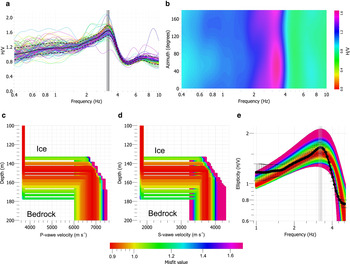
H/V spectra obtained from the passive seismic measurements, using different sensors, at locations P2 (a and c) and P3 (e) on the Pian di Neve glacier (see Figs 1d and 3), and corresponding directional H/V spectra (b, d and f). The two dashed lines in (a), (c) and (e) represent the H/V standard deviation, while the grey areas represent the peak frequency standard deviation, which quantifies the experimental error associated with the average peak frequency value (located at the limit between the dark grey and light grey areas). Even though the measurements were carried out in different periods and using different sensors, the spectra show the same resonance frequency, which is almost azimuth independent (as shown in b, d and f), denoting the absence of 2-D effects.
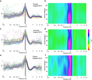
Figures 4b, d, f show the directional H/V spectra, as a function of frequency and azimuth, corresponding to the three sensors. The 0° and 90° directions indicate the North and the East, respectively. These plots clearly indicate that the resonance frequency is almost azimuth independent, denoting the absence of 2-D effects. The peak amplitude shows a maximum at angles ranging from 0° to 30°, highlighting a longitudinal polarization of the recorded wavefield. Moreover, the minimum is located at ~120° in (b) and (d), while in (f) it is less evident and located at ~90°.
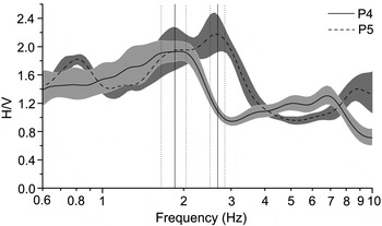
The H/V spectra of the passive seismic records at locations P4 and P5 are displayed in Figure 5. The measured resonance frequencies are 1.85 ± 0.3 and 2.68 ± 0.15 Hz, respectively, denoting a consistent increase moving from P4 to P5. Using the 1-D approximation, this increase of the resonance frequency corresponds to a glacier thinning from 251 ± 43 to 174 ± 12 m. The average ice thickness computed from the seismic section (Fig. 3) within a distance of λ 0/4 from P4 and P5 (which lie right on the seismic line), is 253 ± 5 and 184 ± 5 m. Again, we have an excellent agreement between the results obtained with the two different methods. In particular, this example shows how the HVSR technique may be used to map thickness variations along a glacier.
H/V spectra obtained from the passive seismic measurements, using Trillium sensors, at the locations P4 (solid line) and P5 (dashed line) on the Pian di Neve glacier (see Figs 1d and 3). The grey bands represent the H/V standard deviations, while the vertical solid and dotted lines indicate the resonance frequencies and their associated errors. The resonance frequency recorded at P4 is the same as those recorded at P2 and P3 (see Fig. 4). The figure evidences an increase of the frequency moving from P4 to P5, where we have a consistent reduction of the ice thickness, as can be seen in the imaging section displayed in Figure 3. The directional spectra are not shown because they are very similar to those displayed in Figure 4.
Finally, we adopted the ellipticity inversion to determine the basement velocities and further verify the presence of a rigid bedrock. Because of the large trade-off between depth and velocities, it is convenient to constrain some parameters with other methods in order to stabilize the inversion procedure. Here we use the results obtained from the analysis of the H/V peak frequency and from the active seismic to constrain ice thickness and velocity. However, soft constraints were imposed on these parameters in all the considered sites, in order to also verify the stationarity of the ice seismic velocities. Here, 50 inversion runs with random initial seeds were performed in order to obtain the global minima of the misfit function. Figures 6a–c display the results obtained by inverting the H/V spectrum of Figure 4a, where (a) and (b) show the inverted P- and S-wave vertical velocity profiles, respectively. Figure 6c shows the average H/V spectrum superimposed on the theoretical ellipticity curves of the fundamental-mode Rayleigh wave. The misfits are computed accordingly to the experimental errors, indicated in Figure 6c with the error bars. Considering only misfit values lower than 0.4, the glacier thickness ranges from 240 to 270 m. The P-wave velocity ranges from 3686 to 3724 m s−1 in the ice, and from 5180 to 5610 m s−1 in the underlying bedrock. The S-wave velocity ranges from 1820 to 1870 m s−1 in the ice, and from 3540 to 3800 m s−1 in the underlying bedrock. Inverting the spectra of Figures 4b, c we obtained similar values. These results, showing bedrock velocities higher than those obtained from the imaging procedure, confirm the presence of a rigid bedrock. Moreover, the variability of the ice seismic velocities is well included inside the adopted constraints, in agreement with the ice velocities obtained from the active seismic method.
P-wave (a) and S-wave (b) vertical velocity profiles resulting from the ellipticity inversion of the H/V spectrum shown in Figure 4a. Theoretical ellipticity curves (c) of the fundamental-mode Rayleigh wave, superimposed on the H/V spectrum (black line). The misfits are computed accordingly to the experimental errors, indicated in (c) with the error bars.

3.2. Lobbia glacier
3.2.1. The study site
The Lobbia glacier extends for ~6 km2 on a plateau between the Cresta Croce and Lares summits in the Adamello massif (Fig. 1d), with elevations ranging from 2800 to 3000 m a.s.l.. The glacier is bounded by rock crests on the eastern and western flanks and it opens on steep valleys northwards and on the southern side. Several geophysical surveys were carried out on the Lobbia glacier, including RES (Tabacco and others, Reference Tabacco, Pettinicchio and Veronese1995), gravity measurements (Rosselli and others, Reference Rosselli1997) and active seismic reflection and refraction surveys (Tabacco and others, Reference Tabacco, Pettinicchio and Veronese1995; Levato and others, Reference Levato, Veronese, Lozej and Tabacco1999).
3.2.2. Data acquisition and results
Passive seismic data were acquired using a Guralp sensor at location L as
shown on the map of Figure 1d. This
area was previously investigated by Levato and others (Reference Levato, Veronese, Lozej and Tabacco1999) using the active multichannel seismic method,
estimating an ice thickness of 177 ± 5 m.
Although the lateral extension of the Lobbia glacier is smaller than that of
the Pian di Neve glacier, the 1-D approximation is still valid. Figure 7a displays the H/V spectrum
obtained from the passive seismic measurement, showing a resonance frequency
of $f_0 = 3.22 \pm 0.11{\kern 1pt} {\rm Hz}$
. As in the Pian di Neve case, Figure 7b shows that the resonance
frequency is azimuth independent, with a maximum of the peak amplitude at
~40° and a minimum at ~130°.
$f_0 = 3.22 \pm 0.11{\kern 1pt} {\rm Hz}$
. As in the Pian di Neve case, Figure 7b shows that the resonance
frequency is azimuth independent, with a maximum of the peak amplitude at
~40° and a minimum at ~130°.
H/V spectrum (a) obtained from the passive seismic measurement using a Guralp sensor at the location L on the Lobbia glacier (see Fig. 1d), and corresponding directional H/V spectrum (b). The resonance frequency is almost azimuth independent, denoting the absence of 2-D effects. P-wave (c) and S-wave (d) vertical velocity profiles resulting from the ellipticity inversion of the H/V spectrum shown in (a). Theoretical ellipticity curves (e) of the fundamental-mode Rayleigh wave, superimposed on the H/V spectrum (black line).
The average v
S value in ice, resulting from the
active seismic survey on the Pian di Neve glacier, was used at the Lobbia
site and in all the other considered glaciers, to estimate ice thicknesses
from the H/V peak frequencies. This assumption is justified from the
following considerations: the ice seismic velocities are weakly dependent on
temperature and water content (Thyssen, Reference Thyssen1968; Kohnen, Reference Kohnen1974); in
general, the S-wave velocity in a medium is more sensitive to the presence
of fractures than to fluid content, while P-waves show the opposite behavior
(Carcione and others, Reference Carcione, Gurevich, Santos and Picotti2013);
passive seismic measurements were conducted on flat and barely fractured
glaciers during cold periods to minimize the effect of varying temperature
and water content. Thus, the measured resonance frequency yields a thickness $h = 144 \pm 7{\kern 1pt} \,{\rm m}$
in the 1-D lossless-rigid
approximation.
$h = 144 \pm 7{\kern 1pt} \,{\rm m}$
in the 1-D lossless-rigid
approximation.
The difference between the above two thickness values is considerably higher than the experimental error, but the Lobbia glacier, as well as the adjacent Mandrone glacier, suffered a noticeable ice mass reduction in the last 15 years (Grossi and others, Reference Grossi, Caronna and Ranzi2013). The accelerated retreat of the Mandrone and Lobbia glaciers’ surface at this location is underlined also by the position of the nearby ‘Caduti dell'Adamello’ hut located on the southern slope of the Lobbia Alta summit. The glacier surface in 1916 was at the hut level while presently it is located ~70 m below that position.
In the ellipticity inversion we used the same constraints adopted in the previous case, except for the glacier thickness. Figures 7c–e show the inverted P- (c) and S-wave (d) vertical velocity profiles, and the theoretical ellipticity curves (e) of the fundamental-mode Rayleigh wave. Considering only misfit values lower than 0.95, the glacier thickness ranges from 140 to 155 m. The ice P- and S-wave velocities, as well as the S-wave velocity of the bedrock, are very similar to those obtained on the Pian di Neve glacier, while the bedrock P-wave velocity, ranging from ~6500–7100 m s−1, shows higher values.
3.3. Forni glacier
3.3.1. The study site
Forni glacier is located in the Stelvio National Park, on the Lombardy side of the Ortles-Cevedale massif (Fig. 1b), and it occupies one of the largest Italian glacial valleys. Glaciers in this massif cover an area of ~40 km2 and the Forni glacier alone covers ~12 km2, with elevations ranging from 2600 to 3670 m a.s.l.. Forni glacier is one of the most studied glaciers in the Italian Alps (Senese and others, Reference Senese, Diolaiuti, Mihalcea and Smiraglia2012; Azzoni and others, Reference Azzoni2014), and it has been systematically monitored by the Italian Glaciologic Commission (IGC) over the last 30 years. These periodical observations show that after a slight advance in the period 1970–1987, from 1988 until today the glacier has suffered a persistent retreat, for a total of several hundreds of meters at the front.
3.3.2. Data acquisition
We carried out two mutually perpendicular RES surveys on the Forni glacier and performed passive seismic measurements at the intersection of the two lines (location F in Fig. 1b), using both a Trillium and a Tromino sensor. RES data were collected using a GSSI SIR-2000 system equipped with an unshielded 70 MHz antenna. The antenna was placed on a plastic sledge, with its dipole kept ~0.2 m above the snow surface, in order to achieve consistent coupling. The long axis of the transmitting-receiving dipole was oriented parallel to the scanning direction. Data were recorded in the time domain and in continuous mode setting up a scanning rate of 32 sweeps per second. The signal bandwidth is ~140 MHz delivering a maximum vertical resolution (according to the λ/4 criterion) of ~0.5 m. However, as for the active seismic method, this is a theoretical value and the resolution strongly depends on the S/N ratio. Reference points were located at every 5 m along each profile and these points were later surveyed using a geodetic GPS system.
3.3.3. Results
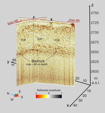
Both the RES profiles, processed using the procedure described in the Appendix, have substantial S/N ratios. The imaged ice/bedrock interface, displayed in Figure 8, is rather sharp although its signature is space-dependent. The estimated experimental error is about one wavelength. In the WE profile (transverse to the ice flow) the bedrock is almost flat and continuous and its top is located at a depth of 77 ± 2 m below the surface. In the SN profile (parallel to the ice flow) the bedrock appears to be dipping southwards. The top reflection ranges from a depth of 70 ± 2 m at the northern edge (upstream) to a depth of 80 ± 2 m at the intersection with the WE profile (downstream). The bedrock response in this last profile is not as clear as in the WE profile, because its signature is unclear and poorly coherent and it is marked by a sudden change in the reflectivity. This change is probably caused by the downward pattern of the antenna that radiates energy on a 90° fan inline and on a 30° fan crossline. The backscattered signal from a deep hummocky target is then averaged over a large sub-elliptical footprint. In general the amount of energy received at the surface is maximum when the major axis of the footprint is elongated transversely to the slope. The reflectivity within the bedrock is poor, because of the low S/N ratio at this depth.
3-D representation of the RES depth sections of the Forni glacier (red dotted lines in Fig. 1b). The passive seismic station (F) was located at the intersection of the two RES lines. The X marks scattering from a hidden crevasse.
The H/V spectra at this site (Fig. 9
shows those obtained with the Trillium sensor) are not as sharp as in the
previous sites. However, as in the Pian di Neve case, results from different
instruments guarantee the reliability of the resonance frequency. The
processed H/V spectra show that the resonance frequencies measured by the
two adopted sensors are identical considering the experimental errors (see
Table 1). The average
resonance frequency is here considerably higher than in the previous cases, $f_0 = 6.1 \pm 1{\kern 1pt} {\rm Hz}$
, resulting in
76 ± 13 m of ice thickness in the 1-D
lossless-rigid approximation. This value is in good accordance with RES
profiling. The directional H/V spectrum displayed in Figure 9b shows that the resonance frequency exhibits
a slight variation with azimuth, probably due to 2-D effects related to the
underlying dipping ice/bedrock interface, with a maximum of the peak
amplitude at ~30° and a minimum at ~120°.
$f_0 = 6.1 \pm 1{\kern 1pt} {\rm Hz}$
, resulting in
76 ± 13 m of ice thickness in the 1-D
lossless-rigid approximation. This value is in good accordance with RES
profiling. The directional H/V spectrum displayed in Figure 9b shows that the resonance frequency exhibits
a slight variation with azimuth, probably due to 2-D effects related to the
underlying dipping ice/bedrock interface, with a maximum of the peak
amplitude at ~30° and a minimum at ~120°.
H/V spectrum (a) obtained from the passive seismic measurements at the intersection of the two RES lines (see Fig. 8) on the Forni glacier (location F in Fig. 1b), by using a Trillium sensor. Corresponding directional H/V spectrum (b), as a function of frequency and azimuth. The resonance frequency exhibits a slight variation with azimuth, probably due to 2-D effects related to the underlying dipping ice/bedrock interface. P-wave (c) and S-wave (d) vertical velocity profiles resulting from the ellipticity inversion of the H/V spectrum shown in (a). Theoretical ellipticity curves (e) of the fundamental-mode Rayleigh wave, superimposed on the H/V spectrum (black line).

In the ellipticity inversion we used the same constraints adopted in the previous cases, except for the glacier thickness. Figures 9c–e show the inverted P- (c) and S-wave (d) vertical velocity profiles and the theoretical ellipticity curves (e) of the fundamental-mode Rayleigh wave. Considering only misfit values lower than 0.5, the glacier thickness ranges from 54 to 73 m. These values are slightly lower than those of the RES profiles, probably because of the data quality and 2-D effects. The seismic velocities in the bedrock range from 4100 to 5200 m s−1 for the P-waves and from 2700 to 3100 m s−1 for the S-waves, confirming again the presence of a rigid bedrock. On the other hand, the seismic velocities in ice are invariant, showing values similar to those obtained in the previous cases.
3.4. La Mare glacier
3.4.1. The study site
The La Mare glacier (Fig. 1c), covering an area of ~3.55 km2 at elevations ranging from 2650 to 3770 m a.s.l., is the largest glacier on the Trentino side of the Ortles-Cevedale massif. It consists essentially of two basins merging downstream into a unique tongue. Between the 1970s and 1980s the front of this glacier advanced by more than 300 m (Carturan and others, Reference Carturan2014), resulting in one of the most significant advances recorded in the Italian Alps in that period. Since then, it has continuously withdrawn, retreating by at least 250 m, with annual values even >40 m. Because of its high altitude, however, in recent years the La Mare glacier has shown a good recovery potential, mainly related to abundant snowfalls above 3200 m.
3.4.2. Data acquisition
We collected two coincident RES and geoelectrical lines (Fig. 1c) and we also carried out two passive seismic measurements along the survey line (locations LM1 and LM2 in Fig. 1c). The RES acquisition system is the same adopted on the Forni glacier. Passive seismic data were recorded using Trillium sensors coupled with the ice at the bottom of 4 m deep holes dug in the snow cover. Geoelectric data were collected using a new generation Multi-Source (MS) geo-resistivimeter (http://www.mpt3d.com – Multy-Phase Technology). The MS system (LaBrecque and others, Reference LaBrecque, Morelli, Fischanger, Lamoureux and Brigham2013) comprises several stand-alone transceivers synchronized via GPS timing and controlled via a 900 MHz radio signal. Each transceiver is capable of handling a maximum of three electrodes. The peculiar and innovative feature of this system, beyond the wireless communication between units, is its capability of transmitting the current simultaneously with multiple dipoles, each one connected to a different transceiver. Field layout was comprised of 12 electrodes spaced 25 m apart. Galvanic contact was achieved by pushing brine-dripping stainless cylinders right into the snow and firn layers. Additional inline dipoles along with longer and external transmitting dipoles were used both to improve the spatial resolution and the depth of penetration of the electric field.
3.4.3. Results
The RES profile, shown in Figure 10a, was collected transversely to the ice flow (Fig. 1c) with its northern edge close to the outcropping rocks. The ice/bedrock interface is concave with a maximum ice thickness in the mid portion of the profile. The ice thickness is 20 ± 2 m at the northern edge while it increases to nearly 30 ± 2 m at a distance of ~310 m. The bedrock signature is homogeneous in the northern and mid portion of the RES scan and it is marked by a sudden change in the reflectivity. In the southern portion of the RES scan the bedrock response appears to be more complex, the ice/bedrock interface gets shallower and the ice-thickness is reduced to 15 ± 2 m at the scan end. A strong reflector, located at a distance of ~400 m (marked with the question mark in Fig. 10a), is probably caused by a stiffer segment of the bedrock or by the presence of a water lens at the bottom of the ice body.
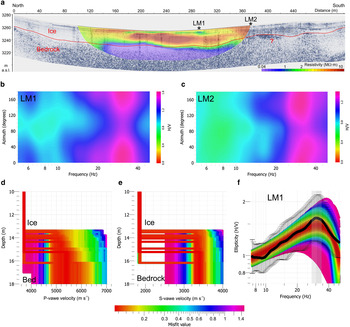
Overlapping ERT and RES depth sections (a) of the La Mare glacier (coincident red and blue dotted lines in Fig. 1c). H/V directional spectra obtained from the passive seismic measurements using Trillium sensors at the locations LM1 (b) and LM2 (c), indicated in (a). The resonance frequency is azimuth independent for LM1 (b), while it exhibits slight variations for LM2 (c) due to the 2-D effects related to the underlying dipping ice/bedrock interface. P-wave (d) and S-wave (e) vertical velocity profiles resulting from the ellipticity inversion of the H/V spectrum shown in (f). Theoretical ellipticity curves (f) of the fundamental-mode Rayleigh wave, superimposed on the H/V spectrum at LM1 (black line).
The MS data were processed and inverted using Electrical Resistivity Tomography (ERT), as described in the Appendix. The ERT section is displayed in Figure 10a, superimposed on the RES scan. These data show a good correlation within the experimental errors, which are estimated to be ~2 and 3 m for the RES and geoelectric methods, respectively. The ice body is almost homogeneous and exhibits very high resistivity values in the order of several MΩ m. Some areas of the MS profile show slightly lower resistivity values, probably because of a higher melting water content. The ice/bedrock interface is clearly visible and it is marked by a sudden drop of the resistivity down to 40 kΩ m. This resistivity value is typical of crystalline rocks or permafrost (Palacky, Reference Palacky and Nabighian1987). Thus it is consistent with the in-situ type of rocks, because the analyzed area is characterized by a prevalence of quartz-phyllites and retrogressed paraschists (Dal Piaz and others, Reference Dal Piaz, Del Moro, Martin and Venturelli1988).
Figures 10b, c display the
directional H/V spectra at locations LM1 and LM2, indicated in Figure 1c. The measured resonance
frequencies show slightly different values, $f_0 = 28 \pm 4{\kern 1pt} {\rm Hz}$
at LM1 and
$f_0 = 28 \pm 4{\kern 1pt} {\rm Hz}$
at LM1 and $f_0 = 30.9 \pm 3.4{\kern 1pt} {\rm Hz}$
at LM2. Using the 1-D lossless-rigid
approximation, justified by the above considerations, these resonance
frequencies give ice thicknesses of 17 ± 3 m and
15 ± 2 m, respectively. Ignoring the 4 m
thick snow cover and considering the S/N ratio, the average glacier
thicknesses computed from the RES and ERT sections within a distance of
λ
0/4 from LM1 and LM2 are
21 ± 2 m and
14 ± 1 m, respectively. Results from the
different methods are thus fully comparable. Moreover, as in the Pian di
Neve case, these results show that the HVSR technique allows the mapping of
thickness variations along a glacier. The directional spectra show that the
resonance frequency is azimuth independent for LM1 (Fig. 10b), while it shows slight variations for LM2
(Fig. 10c), probably due to 2-D
effects caused by the dipping ice/bedrock interface. The peak amplitude
exhibits a maximum at 0° and a minimum at ~90° for both LM1
and LM2.
$f_0 = 30.9 \pm 3.4{\kern 1pt} {\rm Hz}$
at LM2. Using the 1-D lossless-rigid
approximation, justified by the above considerations, these resonance
frequencies give ice thicknesses of 17 ± 3 m and
15 ± 2 m, respectively. Ignoring the 4 m
thick snow cover and considering the S/N ratio, the average glacier
thicknesses computed from the RES and ERT sections within a distance of
λ
0/4 from LM1 and LM2 are
21 ± 2 m and
14 ± 1 m, respectively. Results from the
different methods are thus fully comparable. Moreover, as in the Pian di
Neve case, these results show that the HVSR technique allows the mapping of
thickness variations along a glacier. The directional spectra show that the
resonance frequency is azimuth independent for LM1 (Fig. 10b), while it shows slight variations for LM2
(Fig. 10c), probably due to 2-D
effects caused by the dipping ice/bedrock interface. The peak amplitude
exhibits a maximum at 0° and a minimum at ~90° for both LM1
and LM2.
In the ellipticity inversion we used the same constraints adopted in the previous cases, except for the glacier thickness. Figures 10d–f display the results obtained by inverting the H/V spectrum at LM1, where (a) and (b) show the inverted P- and S-wave vertical velocity profiles, respectively. Figure 10f shows the H/V spectrum at LM1 superimposed on the theoretical ellipticity curves of the fundamental-mode Rayleigh wave. Considering only misfit values lower than 0.15, the glacier thickness ranges from 13 to 16 m (in agreement with the RES and ERT sections), while the seismic velocities of ice and bedrock are similar to those obtained for the Pian di Neve glacier.
3.5. Aletsch glacier
3.5.1. The study site
Aletschgletscher is located in the Bernese Oberland Alps (Fig. 1a), and represents the largest glacier in Europe, covering an area of 86.7 km2. It is 24.7 km long and its elevation ranges from 1555 to 4158 m a.s.l.. In the upper part of the glacier, three major tributaries converge in a 3 km2 plateau named Konkordiaplatz, to form the 20 km-long tongue of Grosser Aletschgletscher. Previous active seismic experiments (Thyssen and Ahmad, Reference Thyssen and Ahmad1969), and drillings in the late 1990s (Hock and others, Reference Hock, Iken and Wangler1999), revealed an overdeepening zone in the Konkordiaplatz with ice thicknesses exceeding 800 m (B90 well, visible in Fig. 1a, reached a maximum depth of 904 m).
3.5.2. Data acquisition and results
RES data were acquired on the Aletsch glacier using an IDS Stream X system equipped with a 25 MHz antenna consisting of separate transmitting and receiving dipoles. Unfortunately, the central frequency is too high and the signal has not enough energy to reach the glacier bottom.
The passive seismic measurements were carried out using Trillium sensors and
provided lower resonance frequencies than in all the previous cases. Figures 11a, c, e display the H/V
spectra obtained, respectively, at the locations A1, A4 and A2, indicated in
Figure 1a. Table 1 summarizes the details about
all the records. The peak frequencies range from
1.06 ± 0.04 Hz outside the Konkordiaplatz
(location A1), to an average frequency of
0.88 ± 0.06 Hz in the Konkordiaplatz. The peak
amplitude shows a maximum at 20° and 0° and a minimum at
120° and 90°, respectively in (b) and (d), implying a
longitudinal polarization of the recorded wavefield. Moreover, in (f) the
maximum and the minimum are located at ~120° and 40°,
respectively. At this site, the glacier thickness is comparable with the
valley half-width $w \approx 700\,{\kern 1pt} {\rm m}$
, and the 1-D approximation is no longer
valid. Using Eqn (1), under
the hypothesis of a rigid bedrock we obtain a thickness of
563 ± 45 m outside the Konkordiaplatz (location
A1), and an average thickness of 820 ± 150 m in
the Konkordiaplatz. These results agree with previous investigations of
Thyssen and Ahmad (Reference Thyssen and Ahmad1969) and Hock
and others (Reference Hock, Iken and Wangler1999), while Eqn (2) gives completely different
values. Hence, in this case the resonances seem to be mainly due to Love
waves or body SH waves. For this reason, ellipticity inversion does not
work. Other reasons are the very large ice thickness and the fact that the
1-D approximation is no longer valid.
$w \approx 700\,{\kern 1pt} {\rm m}$
, and the 1-D approximation is no longer
valid. Using Eqn (1), under
the hypothesis of a rigid bedrock we obtain a thickness of
563 ± 45 m outside the Konkordiaplatz (location
A1), and an average thickness of 820 ± 150 m in
the Konkordiaplatz. These results agree with previous investigations of
Thyssen and Ahmad (Reference Thyssen and Ahmad1969) and Hock
and others (Reference Hock, Iken and Wangler1999), while Eqn (2) gives completely different
values. Hence, in this case the resonances seem to be mainly due to Love
waves or body SH waves. For this reason, ellipticity inversion does not
work. Other reasons are the very large ice thickness and the fact that the
1-D approximation is no longer valid.
H/V spectra (a, c and e) obtained from the passive seismic measurements on the Aletsch glacier, and corresponding directional H/V spectra (b, d and f). The measurements were carried out using Trillium sensors at three different locations: A1, A2 and A4 (see Fig. 1a), respectively. The spectra in (c) and (e) show almost the same resonance frequency, which is lower than in (a). The resonance frequency is almost azimuth independent in (b) and (d), while it exhibits a slight variation in (f), probably due to 2-D effects.
3.6. Whillans Ice Stream
3.6.1. The study site
The WIS, previously known as Ice Stream B, is one of the main ice drainage conduits of the Siple Coast, feeding the Ross Ice Shelf from the interior of the West Antarctic Ice Sheet (WAIS). The ice flow, exceeding 300 m a−1, is characterized by a tidally controlled stick-slip motion, in which long periods of quiescence are followed by short bursts (Bindschadler and others, Reference Bindschadler, King, Alley, Anandakrishnan and Padman2003). Active seismic and RES surface observations (Christianson and others, Reference Christianson, Jacobel, Horgan, Anandakrishnan and Alley2012; Horgan and others, Reference Horgan2012) and subsequent drilling operations (Tulaczyk and others, Reference Tulaczyk2014) confirmed the presence of a shallow active water reservoir beneath the WIS, called Subglacial Lake Whillans (SLW), previously identified by satellite surface elevation observations (Fricker and others, Reference Fricker, Scambos, Bindschadler and Padman2007). Other active and passive seismic experiments (Blankenship and others, Reference Blankenship, Bentley, Rooney and Alley1986; Anandakrishnan and Bentley, Reference Anandakrishnan and Bentley1993), as well as glaciological drilling and instrumentation in the late 1980s and 1990s (Engelhardt and Kamb, Reference Engelhardt and Kamb1997) showed the presence of highly deformable till and water beneath the WIS.
In a recent work, Picotti and others (Reference Picotti, Vuan, Carcione, Horgan and Anandakrishnan2015) inferred the anisotropic and crystal fabric properties of the WIS, by analyzing the active three-component seismic data recorded at the SLW location. They showed that while the shallow firn is isotropic, the underlying ice is weakly anisotropic. In particular, they found that anisotropy is mainly due to crystal orientation fabric, and that the ice is transversely isotropic with a vertical axis of symmetry. This suggests that the principal component of the ice stream movement is basal sliding or deformation in the basal sedimentary layer, rather than deformation in the ice, in agreement with the previous experimental findings evidencing that the subglacial sediments below the WIS are very weak. The average thickness of WIS at the survey location is h = 780 m (Christianson and others, Reference Christianson, Jacobel, Horgan, Anandakrishnan and Alley2012; Horgan and others, Reference Horgan2012), while the shallow firn layer is ~60 m thick (Picotti and others, Reference Picotti, Vuan, Carcione, Horgan and Anandakrishnan2015), implying that the average ice thickness below the firn is ~720 m.
3.6.2. Data acquisition
In this final example we analyzed the H/V spectra obtained from the three-component seismic data recorded on the WIS during the seismic experiment described in Horgan and others (Reference Horgan2012) and Picotti and others (Reference Picotti, Vuan, Carcione, Horgan and Anandakrishnan2015). This experiment, conducted during the 2010–11 Antarctic campaign, involved also the acquisition of RES data, described and analyzed in detail by Christianson and others (Reference Christianson, Jacobel, Horgan, Anandakrishnan and Alley2012). The passive seismic measurements were carried out using 10 Guralp 40-T broadband seismometers with a 40 s corner period, connected to a Reftek station. The sensors were first placed along a longitudinal (along flow) profile, and then arranged in three transverse profiles, as described in Figure 1 of Picotti and others (Reference Picotti, Vuan, Carcione, Horgan and Anandakrishnan2015).
3.6.3. Results
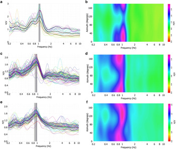
The results obtained from the passive seismic data analysis show two types of H/V spectra. For the first type, the average resonance frequencies are 4.94 ± 0.4 and 5.15 ± 0.93 Hz in the longitudinal and transverse direction, respectively. For the second type, the average resonance frequencies are 1.30 ± 0.17 and 1.23 ± 0.22 Hz in the longitudinal and transverse direction, respectively. For each type of spectrum, considering the experimental errors, the average frequency values are almost identical in the two directions. Figure 12 shows two examples of H/V spectra of the first (a) and second (c) type, obtained along the transverse and longitudinal directions, respectively. The resonance peaks are very sharp, and the corresponding H/V directional spectra (Figs 12b, d) identify that both resonance frequencies and peak amplitudes are azimuth independent. This is in agreement with the results of Picotti and others (Reference Picotti, Vuan, Carcione, Horgan and Anandakrishnan2015), who showed the isotropic character of the firn and excluded the presence of azimuthal anisotropy in the ice due to transversely compressive flow or fractures aligned along a preferential direction.
H/V spectra (a and c) obtained from the passive seismic measurements on the WIS (West Antarctica) by using Guralp sensors. Corresponding directional H/V spectra (b and d), as a function of frequency and azimuth, evidencing that both the resonance frequency and the peak amplitude are azimuth independent.

The measured resonance frequencies are too high and not compatible with the
average ice thickness at the SLW site. However, the resonance peak in the
first type of spectrum can be related to the thickness of the firn layer.
Picotti and others (Reference Picotti, Vuan, Carcione, Horgan and Anandakrishnan2015) computed
the P- and S-wave velocity gradients of the firn using the same methodology
described in the present work. Figure
13 shows the S-wave velocity gradient
v
S(z) and the traveltime
T
0, computed using Eqn (3) along a vertical path
through the entire firn layer. There is a noticeable difference between this
gradient and those characterizing Alpine glaciers, such as the one displayed
in Figure 2b. The computed
traveltime between the surface and the base of the firn is $T_0 = 52.8 \pm 1.8{\kern 1pt} \,{\rm ms}$
, giving a resonance frequency
$T_0 = 52.8 \pm 1.8{\kern 1pt} \,{\rm ms}$
, giving a resonance frequency $f_0 = 5.18 \pm 0.27{\kern 1pt} \,{\rm Hz}$
, which is in good agreement with the
average experimental value (Table
1).
$f_0 = 5.18 \pm 0.27{\kern 1pt} \,{\rm Hz}$
, which is in good agreement with the
average experimental value (Table
1).
S-wave velocity gradient v S(z) (dashed line), as computed in Picotti and others (Reference Picotti, Vuan, Carcione, Horgan and Anandakrishnan2015), and traveltime T 0 (solid line) computed using Eqn (3) along a vertical path between the surface and the base of the firn.

The average resonance frequency of the second type of spectra (see Table 1) is lower but not enough to
be compatible with the ice thickness at the site, under the hypothesis of a
rigid bedrock. In fact, considering that the average S-wave velocity of the
whole ice column is $v_{{\rm S}1} = 1940 \pm 20{\kern 1pt} \,{\rm m}{\kern 1pt} {\rm s}^{ - 1} $
(Picotti and others, Reference Picotti, Vuan, Carcione, Horgan and Anandakrishnan2015) and that the lateral extension
of the WIS is much larger than the ice thickness, a 720 m thick ice
stream should have a fundamental resonance frequency of ~0.67 Hz,
while the average experimental resonance frequency is
1.27 ± 0.19 Hz. This discrepancy is due to the
fact that the lossless-rigid approximation is not valid in this case. As
explained earlier, several authors suggest that the subglacial material
beneath WIS consists of highly dilated and deforming sediments. In
particular Blankenship and others (Reference Blankenship, Bentley, Rooney and Alley1986), using the active seismic method, estimated that the
S-wave velocity and density of the basal sediments are
$v_{{\rm S}1} = 1940 \pm 20{\kern 1pt} \,{\rm m}{\kern 1pt} {\rm s}^{ - 1} $
(Picotti and others, Reference Picotti, Vuan, Carcione, Horgan and Anandakrishnan2015) and that the lateral extension
of the WIS is much larger than the ice thickness, a 720 m thick ice
stream should have a fundamental resonance frequency of ~0.67 Hz,
while the average experimental resonance frequency is
1.27 ± 0.19 Hz. This discrepancy is due to the
fact that the lossless-rigid approximation is not valid in this case. As
explained earlier, several authors suggest that the subglacial material
beneath WIS consists of highly dilated and deforming sediments. In
particular Blankenship and others (Reference Blankenship, Bentley, Rooney and Alley1986), using the active seismic method, estimated that the
S-wave velocity and density of the basal sediments are $v_{{\rm S}2} = 150 \pm 10{\kern 1pt} \,{\rm m}{\kern 1pt} {\rm s}^{ - 1} $
and
$v_{{\rm S}2} = 150 \pm 10{\kern 1pt} \,{\rm m}{\kern 1pt} {\rm s}^{ - 1} $
and $\rho _2 \,{\approx}\, 2016{\kern 1pt} \,{\rm kg}{\kern 1pt} {\rm m}^{ - 3} $
, respectively. The density of pure ice
being
$\rho _2 \,{\approx}\, 2016{\kern 1pt} \,{\rm kg}{\kern 1pt} {\rm m}^{ - 3} $
, respectively. The density of pure ice
being $\rho _1 \,{\approx}\, 917{\kern 1pt} \,{\rm kg}{\kern 1pt} {\rm m}^{ - 3} $
, it follows that the impedance contrast
at the bed is α ≥ 1. As shown
by Carcione and others (Reference Carcione, Picotti, Francese, Giorgi and Pettenati2017), in
the case of stiff over soft medium, the fundamental frequency coincides with
a minimum of the S-wave transfer function, and it is
f
0 = f
1/2,
where f
1 is the experimental resonance
frequency. Hence, using the 1-D approximation we obtain a thickness of
764 ± 122 m, which is in accordance with
previous investigations of Horgan and others (Reference Horgan2012) and Christianson and others (Reference Christianson, Jacobel, Horgan, Anandakrishnan and Alley2012). This final example shows that
bedrock deformability must be taken into account to obtain a reliable
estimate of the glacier thickness.
$\rho _1 \,{\approx}\, 917{\kern 1pt} \,{\rm kg}{\kern 1pt} {\rm m}^{ - 3} $
, it follows that the impedance contrast
at the bed is α ≥ 1. As shown
by Carcione and others (Reference Carcione, Picotti, Francese, Giorgi and Pettenati2017), in
the case of stiff over soft medium, the fundamental frequency coincides with
a minimum of the S-wave transfer function, and it is
f
0 = f
1/2,
where f
1 is the experimental resonance
frequency. Hence, using the 1-D approximation we obtain a thickness of
764 ± 122 m, which is in accordance with
previous investigations of Horgan and others (Reference Horgan2012) and Christianson and others (Reference Christianson, Jacobel, Horgan, Anandakrishnan and Alley2012). This final example shows that
bedrock deformability must be taken into account to obtain a reliable
estimate of the glacier thickness.
Ellipticity inversion is not feasible in this case because of the remarkable ice thickness and the strong velocity inversion at the bed. However, Picotti and others (Reference Picotti, Vuan, Carcione, Horgan and Anandakrishnan2015) determined the firn and ice S-wave velocity structure down to a depth of ~300 m by inverting the Love and Rayleigh wave dispersion curves from active seismic data.
4. DISCUSSION
The examples presented in this work clearly show that ambient noise measurements and the HVSR technique can effectively be applied to map the thickness of glaciers, in a wide range from a few tens of meters to over 800 m. Even if the experimental error for thicknesses exceeding 700–800 m becomes large, this methodology provides a rough but reliable estimation of the average thickness within λ 0/4.
4.1. Limits of applicability
The limits of this technique in glacial environments are evident in the last example. The first limit regards the S-wave impedance contrast at the glacier bottom. As pointed out by different authors (e.g. Bonnefoy and others, Reference Bonnefoy-Claudet, Köhler, Cornou, Wathelet and Bard2008), a reliable estimate of the fundamental resonant frequency from the H/V spectra strongly depends on the magnitude of the S-wave impedance contrast between the shallow layer and the basement. Moreover, while the basal impedance contrast can be ignored in presence of a rigid bedrock, when the subglacial material consists of highly dilated and deforming sediments this results in an incorrect estimate of the glacier thickness. In other words, the lossless-rigid approximation is no longer valid and bedrock deformability must be taken into account. The second limit is related to how the seismometer is coupled with the glacier surface. When the firn layer is very thick, it represents a waveguide which traps most of the energy carried by ambient noise waves. This effect is also the cause of the resonance frequency in the firn.
Another limitation of this technique is that often the seismometers might be strongly misaligned while recording, which could lead to large errors in HVSR estimations. Several long recordings (see Table 1) provided sufficient insight to investigate such potential misalignments in the seismic sensors. For example, while on the Lobbia glacier there was no snow and the sensor was placed right on the glacier top, on the Aletsch glacier the abundance of snow allowed us to protect the sensor (location A4) at the bottom of a deep hole dug in the firn. In the first case we verified that misalignments started to affect the recorded data after ~7 h, while in the second case there is no evidence of misalignments in the whole record. This different behavior of the two instruments might be due to the fact that in the second case the sensor was more protected from daily temperature and weather changes. These two examples show how a properly coupled and insulated sensor minimizes misalignments and results in high quality H/V spectra.
In general, we observed that the HVSR data quality is better for thick glaciers than for thin glaciers. In particular, the HVSR curves of thick glaciers (e.g. Pian di Neve, Lobbia, Aletsch and WIS) exhibit a better stability in time, while for thin glaciers (e.g. Forni and La Mare) we observe a higher time-dependent variability. This is primarily due to the fact that thin glaciers are excited by high-frequency waves, which are produced by a number of sources of many different natures, including changeable weather conditions (e.g. the wind), human activities, etc. On the other hand, the fundamental resonances of thick glaciers involve low-frequency waves, which are produced by almost time-invariant broad sources (e.g. the oceans).
4.2. H/V directional spectra and crevasse patterns
The directional H/V spectra shown in the various examples exhibit some interesting characteristics, which can be related to typical glacier features. The motion of Alpine glaciers is generally characterized by strong transverse and longitudinal velocity gradients, causing cracks and the development of different types of crevasses (Hambrey, Reference Hambrey1994). Extensive or compressive flow within the ice generates transverse and longitudinal crevasses, respectively, while shear at the valley walls generate marginal crevasses, forming herring-bone patterns bending up-glacier in the flow direction (see Fig. 14).
Crevasse diagram in a typical Alpine glacier showing different flow states (modified from Hambrey, Reference Hambrey1994). Solid lines indicate the crevasses, while the normal arrows indicate the maximum tensile stresses. Marginal crevasses form herring-bone patterns pointing up-glacier. Grey stars indicate different passive seismic measurement sites, in which the sensor is oriented along the flow direction. The orientation angle of the crevasse patterns generally increases going from up-glacier towards down-glacier.

A fractured medium behaves as an anisotropic medium when the wavelength is much larger than the distance between fractures (e.g. Santos and others, Reference Santos, Picotti and Carcione2012, and references therein). Due to the large wavelengths of ambient noise, this condition is generally valid for passive seismic measurements on Alpine glaciers, which should be sensitive to the presence of crevasses. Carcione and others (Reference Carcione, Picotti and Santos2012) considered both dry and wet fractures in a viscoelastic medium, showing that the attenuation of P waves is maximum in the azimuthal direction normal to the fracture system (while S waves show a different behavior), where the H/V spectra should exhibit a maximum of the peak amplitude. On the other hand, the attenuation of P-waves is minimum in the direction parallel to the fracture system, where the H/V spectra should exhibit a minimum of the peak amplitude. These results suggest a physical interpretation of the directional H/V spectra obtained in this work. Let us consider a sensor placed towards the middle of a glacier. If the sensor is oriented in the direction of the flow, a maximum of the H/V spectral ratio is expected around that direction, when in presence of transverse crevasses. However, because of the large wavelengths involved in these kind of experiments, the recorded microtremors might be sensitive also to the presence of marginal crevasses towards the sides, and for this reason a minimum of the H/V spectral ratio is expected between 90° and 150° (and a maximum between 0° and 60°). The results shown in this work clearly exhibit these two features. In fact, almost all the directional H/V spectra show a maximum located between 0° and ~30°–40°. Considering possible asymmetries in the crevasse patterns present on the two sides of a glacier, this means that the recorded wavefield is polarized in the flow direction. The minima are instead located between ~90° and 140°, denoting the presence of transverse and/or herring-bone crevasse patterns. For example, the minimum at ~90° in the directional spectra of Figures 10b, c denotes the presence of transverse crevasses on the La Mare glacier, which is plausible because this glacier is located in an ice accumulation area. The Pian di Neve glacier shows similar characteristics, but the spectra of Figures 4b, d indicate also the presence of marginal crevasses. In the Aletsch glacier case, outside the Konkordiaplatz, the spectrum of Figure 11b denotes the presence of marked marginal crevasses. Similar features are observed for the Lobbia and Forni glaciers. In all the considered cases, the directional spectra highlight a longitudinal polarization of the recorded wavefield. Inside the Konkordiaplatz the situation is more complex because of the convergence of three large glacier tributary tongues.
4.3. Seismic properties of bedrock
The HVSR technique can be used to infer the seismic properties of the bedrock by considering different features of the H/V spectra, namely, the shape, amplitude and frequency of the resonance peaks and the frequency of the troughs.
When the ice thickness can be determined using other methods, the technique allows to easily distinguish between a rigid bedrock or a deformable basement (or water) underneath the ice body. For example, in the WIS case a minimum is located at the fundamental resonance frequeny f 0, confirming that the basement consists of highly deformable sediments and water. On the other hand, in the Pian di Neve case the peak amplitude is located at f 0, confirming the presence of a rigid bedrock and supporting the results of active seismic about the nature of the layer at the glacier bottom. Moreover, in the case of rigid bedrock the S-wave impedance of the basement can be obtained from the ellipticity inversion. If the ice thickness is unknown, however, we showed that the peak frequency provides a reliable estimation of the ice thickness (in the lossless-rigid approximation), which can be used to constrain and stabilize the inversion procedure. Nevertheless, the results obtained using ellipticity inversion have to be carefully evaluated.
Several authors (e.g. Bonnefoy and others, Reference Bonnefoy-Claudet, Köhler, Cornou, Wathelet and Bard2008) analyzed the propagation of surface and body waves at different sites consisting in sedimentary basins overlying bedrock, indicating a considerable variability of the peak amplitudes regardless of the acoustic impedance contrast at the base of the sediments. They concluded that there should be a relationship between the peak amplitude and the impedance contrast, because if the contrast is strong, surface waves are better confined within the shallow soft layer (the ice, in our case). However, to our knowledge there is no validated formula that uniquely correlates the spectral H/V peak amplitude with the basal impedance contrast.
Additional information about the seismic properties of the bedrock can be obtained by analyzing not only the peaks but also the troughs in the H/V spectra. Let us consider a soft soil layer lying upon a hard rock half-space. Tuan and others (Reference Tuan, Scherbaum and Malischewsky2011), assuming that the propagation of Rayleigh surface waves is dominant, derived a relationship between the peak (f 0) and trough (f 1) frequency ratio f 1/f 0 and the key parameters of the model, i.e., the Poisson's ratio of the soil and the S-wave impedance contrast between the soil and the rock. For example, in the Pian di Neve case we have a marked peak/trough structure with f 1/f 0 ≈ 1.6. The average Poisson's ratio of the ice resulting from the active seismic experiment is 0.331, while the average v P of the crystalline bedrock is ~4500 m s−1. As explained before, assuming a ratio v P/v S ≈ 1.6 (Moos and Zoback, Reference Moos and Zoback1983), the average v S of the crystalline bedrock is ~2812 m s−1. Moreover, assuming an average density of ~917 and 2700 kg m−3 for the ice (Picotti and others, Reference Picotti, Vuan, Carcione, Horgan and Anandakrishnan2015) and for the fractured quartz-diorite (Hughes, Reference Hughes1982), respectively, we obtain an S-wave impedance ratio α 1/α 2 of ~0.22 between the ice (α 1) and the bedrock (α 2). In this computation we ignore the presence of the thin sedimentary layer at the glacier base, its thickness being much smaller than λ 0. This value of α 1/α 2 is in good agreement with the value provided by the map displayed in Figure 2 of Tuan and others (Reference Tuan, Scherbaum and Malischewsky2011).
Since the H/V spectra presented in this study often exhibit the peak/trough structure (e.g. the Pian di Neve, Lobbia and Forni glaciers), we suggest that a typical mechanism influencing the HVSR method on glaciers is the propagation of Rayleigh waves. However, in many cases (e.g. Aletsch glacier, La Mare glacier, and the WIS), the troughs are less prominent or totally absent (e.g. Fig. 11) suggesting that the resonances are probably due to the propagation of Love waves or body SH waves.
5. CONCLUSIONS
The HVSR technique has been tested on passive seismic data from several Alpine glaciers in the Adamello and Ortles-Cevedale massifs (Italy) and in the Bernese Oberland Alps (Switzerland), and from the WIS (West Antarctica). Results were validated using active seismic, RES and geoelectric methods, meeting modern standards and widely used in exploration geophysics. The resonance frequency in the H/V spectra correlates well with the ice thickness at each considered site, in a wide range from a few tens of meters to over 800 m. In almost all the examined cases, the directional H/V spectra show that the resonance frequency is nearly azimuth independent while the maximum peak amplitude lies at low azimuths, denoting a longitudinal polarization of the recorded wavefield. Moreover, the peak amplitude exhibits a minimum that correlates well with the orientation of typical crevasse patterns in a glacier. In addition, the H/V curves often exhibit the peak/trough structure (e.g. the Pian di Neve, Lobbia and Forni glaciers), suggesting that the propagation of Rayleigh waves drives the shape of the H/V spectra. However, in some cases the peak/trough structure is less evident (e.g. the Aletsch glacier), indicating a predominance of Love waves, which should be taken into account when width and depth of the investigated glacier are comparable. The analysis of three-component seismic data acquired on the WIS (West Antarctica) showed that the results of this technique have to be carefully evaluated when the seismometers are coupled with a thick firn layer at the surface, or when highly deformable sediments are present underneath the ice body. In case the propagation of Rayleigh surface waves is dominant and the glacier thickness can be constrained, ellipticity inversion of the H/V spectra allows us to infer the seismic properties of the basement in the presence of 1-D structures and a rigid bedrock.
This work shows that the HVSR technique provides a cost-effective alternative to active-source geophysical methods, that have been used as the standard for several years to map glacier thicknesses and to estimate bedrock properties. The minimal logistics involved in the HVSR measurements allow for mass-balance studies also in extreme environments (e.g. Himalaya and Karakoram glaciers), where the common methods are generally impractical. A single operator in a working day could easily carry console and seismometer and sample glacier geometry at several locations. In addition seismic, geoelectric and RES methods often generate ambiguous or unsatisfactory results for different reasons, for example, coupling problems, wave scattering, high amplitude attenuation in the shallow layers and when the target depth is beyond the imaging capability. In these cases, the HVSR methodology may provide reliable thickness estimates and resolve ambiguities, notwithstanding that the experimental error could become large for thicknesses exceeding 700–800 m. Finally, when the ice thickness is known from other sources, the method allows easy discrimination between a rigid bedrock and a deformable basement (or water) beneath the ice body.
ACKNOWLEDGEMENTS
We dedicate this paper to the memory of Marco Mucciarelli, who encouraged us to perform this study. This work was supported by the Italian National Program of Antarctic Research (PNRA–WISSLAKE Project) and the US National Science Foundation (WISSARD Program–NSF 0944794, 0632198, and 0424589). We thank Alessandro Vuan for his constructive suggestions.
APPENDIX A
Here we summarize the analytical techniques adopted for the geophysical imaging methods, i.e., active seismic, RES and geoelectric methods.
ACTIVE SEISMIC
The active seismic data were analyzed employing the following computational sequence: seismic data processing, traveltime tomography and imaging. The adopted seismic data processing was aimed at increasing the signal-to-noise (S/N) ratio by reducing the coherent noise (i.e. surface waves, etc.) and to improve the lateral coherency of the reflectors of interest (Yilmaz, Reference Yilmaz2001). The processing included: band-pass filtering and Trimmed-mean dynamic dip filtering (e.g. Giustiniani and others, Reference Giustiniani, Accaino, Picotti and Tinivella2008) to eliminate the random and coherent noise (ground-roll and direct waves); predictive deconvolution for the wavelet compression; amplitude recovery, to compensate for geometrical spreading and adsorption; stacking velocity analysis and stacking. Two types of traveltime tomography techniques were employed to invert the diving-wave first breaks of the shallow refraction dataset and the reflected arrivals from the glacier bottom of the primary line. The first technique performs a traveltime inversion of P and S diving waves in the firn, by using the Herglotz-Wiechert inversion method (e.g. King and Jarvis, Reference King and Jarvis2007; Picotti and others, Reference Picotti, Vuan, Carcione, Horgan and Anandakrishnan2015), applied for the first time on ice to data from Antarctica by Kirchner and Bentley (Reference Kirchner and Bentley1979). This procedure allowed us to determine the vertical velocity gradient down to ~12 m depth, where the medium is pure ice. Below the firn, an iterative imaging technique involving P-wave residual move-out analysis, tomography and pre-stack depth migration (Yilmaz, Reference Yilmaz2001; Giustiniani and others, Reference Giustiniani, Accaino, Picotti and Tinivella2009) was used to generate a vertical seismic section of the glacier, basal sediments and underlying bedrock.
RADIO-ECHO SOUNDING
RES data were entirely processed in the open-source environment of the CWP Seismic Unix package (Stockwell, Reference Stockwell1999). The base processing flow included: zero time correction, to align the ground impact (air/snow interface reflection) of each trace at zero time; bandpass filtering, to improve the S/N ratio; background removal, to remove the low frequency envelope, the so-called ‘wow’, a typical low frequency noise caused by the direct-wave arrival; and amplitude recovery. In some cases the typical banding of RES scanlines overpowered the reflected signal. This ringing appeared to be coupling-dependent (Carturan and others, Reference Carturan2013; Seppi and others, Reference Seppi2015) and different segments of the same profile showed a different ringy character. The standard running-average filter, generally very effective in removing the bands (e.g. Francese and others, Reference Francese, Galgaro and Grespan2004), was successful only in case of very narrow trace windows. The drawback in computing the mean with just few traces was the severe attenuation of both noise bands and horizontal reflectors (Forte and others, Reference Forte, Pipan, Francese and Godio2015). A different approach was then required to filter out the ringing. An automatic routine was coded for this specific purpose. The scanline was split in subscans with homogeneous ringing and each subscan was processed separately before merging the data onto the original scanline. The approach proved to be successful and the S/N ratio was definitely improved (Francese and others, Reference Francese2015).
GEOELECTRIC
Apparent resistivity data were analyzed and found to be of good quality. The reciprocal measurements exhibited a minor deviation, which confirmed the reliability of the dataset. Few points were removed from the dataset prior to inverting from apparent to true resistivity model. The mesh consists of a tetrahedral grid with a cell size of 10 m and the model was initiated assigning a constant resistivity value to each cell. The adopted ERT algorithm uses a smoothness-constrained approach under the Occam assumptions (e.g. Cardarelli and Fischanger, Reference Cardarelli and Fischanger2006) with a careful re-weighting of the inversion parameters (Morelli and LaBrecque, Reference Morelli and LaBrecque1996). The resulting inversion misfit was <5% for the majority of the data points, providing fully-interpretable results.


 Open access