2.1 Environment

Time is continuous. Agents are risk-neutral, infinitely lived and discount the future at a rate $r$ . There are three types of agents: households, developers and realtors. Households either own a home, search for a house (i.e. they are buyers), or choose not to participate in the market. Developers may enter the housing market and build a new home at a cost $k$ if not enough existing houses are listed for sale by households through separations. Upon building a house, developers post a vacancy and search for buyers. Houses are identical, regardless of whether they are old or newly built. To capture depreciation in a tractable way, houses are destroyed at an exogenous rate $\delta$ .

It takes time for buyers to find a house and for sellers to sell their home. We capture these search frictions in the housing market by assuming a matching function $M(b,v)$ , where $b$ is the measure of buyers and $v$ the measure of vacancies or houses for sale—we use both terms interchangeably. The matching function satisfies the usual properties: it is increasing in each of its terms, concave and displays constant returns to scale. Let $\theta \equiv b/v$ denote the housing market tightness. The matching function implies that buyers find homes at a rate $m(\theta ) \equiv M(b,v)/b=M(1,\theta ^{-1})$ and that sellers find buyers at a rate $\theta m(\theta ) = M(b,v)/v=M(\theta ,1)$ . As market tightness increases, the home-finding rate for buyers $m(\theta )$ decreases and the finding rate for sellers $\theta m(\theta )$ increases. Intuitively, an increase in market tightness implies that vacancies are relatively more scarce, so it becomes harder for buyers to find a house, but easier for a seller to find a buyer. In addition to these flows, some homeowners become separated from their house at an exogenous rate $s$ . This separation shock captures that the household may need to relocate because of their job, need to move to a different type of home or area, and so on. Once a separation shock occurs, households list their house for sale.

There is free entry of both buyers and sellers. Given free entry of buyers, households keep entering the market until the value of becoming a buyer equals zero, the value of their outside option.Footnote ⁵ Similarly, free entry of sellers implies that sellers enter the market until the value of a vacancy equals the construction cost $k$ , regardless of whether the house is newly built or existing (all houses are identical). As is common in markets with search frictions, there are rents from matching. We assume that prices are determined by Nash Bargaining (Nash and John, Reference Nash and John1950; Rubinstein, Reference Rubinstein1982), where $\beta$ denotes the seller’s bargaining strength.Footnote ⁶ Once a buyer and a seller are matched, the buyer pays the price $p$ to the seller and begins enjoying a utility flow $\varepsilon$ from owning a house.

Households must secure the services of a realtor to start searching for a house. Searching for houses is costly for the realtor. Her cost of servicing $b$ buyers is given by $\bar {c} b^{\gamma +1}/(\gamma +1)$ , which is consistent with many findings in the real estate literature (Sirmans and Turnbull, Reference Sirmans and Turnbull1997). In exchange for her services, the realtor charges a fee $c^B$ , so her revenue is $b c^B$ . Assuming a competitive market, the realtor’s problem is to maximize her net present value of profits, $\int _t^{\infty }e^{-r(v-t)}[b(v) c^B(v) - \bar {c} b(v)^{\gamma +1}/(\gamma +1)]dv$ , with respect to $b(v)$ , the measure of buyers she provides the service to. Absent shocks, the realtor’s problem of maximizing the net present value of all future profits reduces to a static problem of maximizing profits per unit of time. Thus, profit maximization implies that the fee is given by $c^B(b)=\bar {c} b^{\gamma }$ , which is increasing in the number of buyers.Footnote ⁷ Intuitively, $c^B(b)$ captures search costs such as arranging and scheduling viewings, driving to view houses or locating properties that match buyers’ preferences. In reality, buyers incur some of these costs themselves, but to simplify the exposition we assume that the realtor bears all the costs and then charges a fee $c^B(b)$ . Assuming instead that buyers incur all costs themselves, and that costs are increasing in the number of buyers due to congestion, gives the exact same results. This endogenous entry mechanism generates an upward-sloping Beveridge Curve, and accounts for the housing market stylized facts qualitatively and quantitatively (Gabrovski and Ortego-Marti, Reference Gabrovski and Ortego-Marti2019). Finally, sellers incur search flow cost $c^S$ until they find a buyer.Footnote ⁸

2.2 Decentralized equilibrium

Let $H$ , $B$ and $V$ denote the value functions of a homeowner, a buyer and a vacancy. They satisfy the Bellman equations

(1) \begin{align} & rB=\max \{0,-c^B(b) + m(\theta )(H - B - p) )\} , \end{align}

(2) \begin{align} & rH= \varepsilon - s(H-V-B)-\delta (H-B) . \end{align}

Intuitively, buyers can choose whether to enter the housing market. When they search for a house, they incur flow costs $c^B(b)$ . At a rate $m(\theta )$ , they find a house, pay the house price $p$ and become a homeowner, which carries a net gain $H-B-p$ . A homeowner derives a utility $\varepsilon$ from owning a house. At a rate $s$ a separation shock occurs, and the household lists her house for sale, which has a value $V$ , and decides whether to become a buyer. At a rate $\delta$ the house is destroyed, which implies a net loss of $H-B$ . Similarly, the seller’s Bellman equation is given by

(3) \begin{align} & rV=-c^S + \theta m(\theta )(p- V) -\delta V . \end{align}

Sellers incur flow costs $c^S$ while they search. At a rate $\theta m(\theta )$ , they meet a buyer and enjoy net capital gains $p-V$ . The vacancy is also subject to a destruction shock at a rate $\delta$ .

Because of the frictional nature of the housing market, a match between a buyer and seller generates a positive surplus. We assume that the two parties split this surplus according to Nash Bargaining. Let $S^B \equiv H-B-p$ and $S^S \equiv p-V$ denote the surpluses of the buyer and seller, and let $S \equiv S^B+S^S$ denote the total surplus. Prices solve the following Nash Bargaining problem

(4) \begin{align} p=\mathop{\mathrm{arg\,max}}\limits_{p} \left (S^B \right )^{1-\beta } \left (S^S \right )^{\beta } . \end{align}

The first order condition to the above problem yields $(1-\beta ) S^S= \beta S^B$ . In particular, the above sharing rule implies that the buyer extracts a fraction $1-\beta$ of the surplus and the seller a fraction $\beta$ , i.e. $S^B = (1-\beta ) S$ and $S^S=\beta S$ . As a consequence both the buyer and seller agree on when the trade is beneficial, i.e. $S^B \geq 0$ if and only if $S^S \geq 0$ , and if and only if $S\geq 0$ .

Free entry implies that sellers enter the market until the value of a vacancy covers the construction costs $k$ , i.e. $V=k$ . On the buyer’s side, households participate in the market until the value of being a buyer $B$ equals the value of their outside option, which we normalize to 0, i.e. $B=0$ . Combining the Bellman equations for the buyer and seller (1) and (2) with the free entry condition for sellers implies

(5) \begin{align} & S^B = \frac {\varepsilon + s k }{r+s+\delta } - p , \end{align}

(6) \begin{align} & S^S=p-k . \end{align}

Combining the above surpluses with the Nash bargaining rule gives the equilibrium price (PP) condition

(7) \begin{align} & \text{(PP):} \ \ \ \ \ \ p = k + \beta \left (\frac {\varepsilon + s k }{r+s+\delta }-k \right ) . \end{align}

Intuitively, due to Nash Bargaining sellers are compensated for their outside option, $k$ , and receive a share $\beta$ of the surplus.Footnote ⁹

Free entry of sellers, together with the Bellman equation for a vacancy (3) gives the Housing Entry (HE) condition

(8) \begin{align} & \text{(HE): }\ \ \ \ \ \ \ \frac {(r+\delta )k+c^S}{\theta m(\theta )} = p-k . \end{align}

The left hand-side of the above equation captures the seller’s expected cost from searching for a buyer: the search cost $c^S$ and the user cost $(r+\delta )k$ for the expected duration of the vacancy $1/(\theta m(\theta ))$ . The right-hand side corresponds to the seller’s surplus. The HE condition reflects that developers keep entering the market until the profits from selling the house are just enough to cover the expected cost of finding a buyer. Thus the (HE) condition governs entry of sellers in equilibrium.

Free entry of buyers gives the Buyer’s Entry (BE) condition

(9) \begin{align} & \text{(BE): }\ \ \ \ \ \ \ \frac {c^B(b)}{m(\theta )} = (1-\beta ) \left (\frac {\varepsilon + (r+\delta )k}{r+\delta + s} \right ). \end{align}

Intuitively, buyers keep entering the market until the marginal buyer’s expected cost of finding a home equals the buyer’s surplus of being a homeowner, which equals the present discounted value of the return $\varepsilon$ net of the user cost $(r+\delta )k$ , using the effective discount $r+s+\delta$ .

The PP and HE conditions determine the equilibrium market tightness $\theta$ . Given the equilibrium $\theta$ , the BE condition yields the equilibrium measure of buyers $b$ . It is straightforward to verify that the equilibrium exists and is unique. This environment yields an upward-sloping Beveridge Curve, which corresponds to the BE curve. Intuitively, as more sellers enter the market, buyers find it more desirable to enter because they can find houses more quickly. Hence, buyers and vacancies are positively correlated and the BE curve is upward-sloping.

The equilibrium is depicted graphically in figures 1a, b. Figure 1a depicts the HE condition and the price relationship PP given by (7) and (8). The HE condition captures that as house prices increase it becomes more profitable to post a vacancy. This leads to more entry of sellers and a lower market tightness. The PP condition comes from Nash Bargaining between buyers and sellers. The equilibrium price $p^{\ast }$ and market tightness $\theta ^{\ast }$ are given by the intersection of both curves. The equilibrium market tightness $\theta ^{\ast }$ in figure 1a describes a straight line in the vacancies-buyers space in figure 1b, which we denote as the HE condition. The BE curve in figure 1b corresponds to the BE condition (9). The BE curve captures that as the ratio of vacancies to buyers increases buyers find houses faster, which leads to an increase in the entry of buyers.

Figure 1. Equilibrium in the housing market.

2.3 The social planner’s allocation

The social planner faces two externalities. In addition to the usual congestion externality in markets with search frictions, the decentralized equilibrium is inefficient because buyers do not internalize the effect their entry has on other buyers’ search costs. We refer to this additional externality as the participation externality. Let $\tilde {h}$ and $c$ denote the number of homeowners and construction (the number of newly built houses). The planner’s problem is given by

(10) \begin{align} & \max _{\theta , c} \int _{0}^{\infty } e^{-rt}\left [\varepsilon \tilde {h}- v \theta c^B(v \theta )-vc^S-ck\right ]\,\text{d}t , \end{align}

subject to

(11) \begin{align} & \dot {v}=c+sh-\delta v - v\theta m(\theta ) , \end{align}

(12) \begin{align} & \dot {\tilde {h}}=v\theta m(\theta )-(s+\delta )\tilde {h}. \end{align}

Setting up the Hamiltonian and using the first order conditions gives the following solution for the planner’ allocation at steady state

(13) \begin{align} & \frac {(r+\delta )k+c^S}{\theta m(\theta )}={\alpha }\left (\frac {\varepsilon +sk}{r+s+\delta }-k\right ), \end{align}

(14) \begin{align} & \frac {c^B(b)}{m(\theta )}={\left (\frac {1-\alpha }{1+\gamma }\right )}\left (\frac {\varepsilon +sk}{r+s+\delta }-k\right ), \end{align}

where $\alpha \equiv - m'(\theta )\theta /m(\theta )$ denotes the elasticity of the matching rate. The appendix provides the derivations and shows that the above conditions are necessary and sufficient. Equations (13) and (14) are the counterpart of the equilibrium conditions (8) and (9) in the decentralized economy. Comparing the decentralized allocation with the optimal one shows that the HMP condition does not restore efficiency. More specifically, restoring efficiency in the decentralized equilibrium requires

(15) \begin{align} \beta =\alpha \quad \text{and} \quad 1-\beta =\frac {1-\alpha }{1+\gamma }. \end{align}

The first condition $\beta =\alpha$ corresponds to the standard HMP condition. If HMP holds, the decentralized equilibrium is efficient if and only if $\gamma =0$ , i.e. there is no entry of buyers. As soon as there is free entry of buyers, the equilibrium is inefficient because the endogenous entry of buyers generates a participation externality.Footnote ¹⁰ Intuitively, when there is no buyer entry the only externality is the congestion externality, which can be internalized if the two parties share the surplus in the appropriate fractions, i.e. the seller receives a share $\alpha$ and the buyer receives the rest. With endogenous entry of buyers, however, the participation externality manifests itself through increased search costs for buyers. As a result, the planner finds it optimal to disincentivize entry by giving buyers only a share $(1-\alpha )/(1+\gamma )$ of the surplus and leaving the remaining $\gamma (1-\alpha )/(1+\gamma )$ fraction of the surplus “on the table.” Thus, at least two housing market policies are required to eliminate the two externalities and restore efficiency: one policy to set the fraction of surplus that is left “on the table” (i.e. eliminate the participation externality), and one to set the sharing rule for the remainder of the surplus (i.e. eliminate the congestion externality).Footnote ¹¹

3.1 The model with housing policies

We consider four policies. First, homeowners pay property taxes $\tau _p$ on their home. Second, buyers pay taxes $\tau _b$ when they purchase a house. Third, sellers pay a tax $\tau _s$ upon selling the house, which we assume applies to the capital gains $p-V$ . Finally, construction may be taxed or subsidized at a rate $\tau _k$ , where $\tau _k \gt 0$ corresponds to a tax on construction and $\tau _k \lt 0$ to a subsidy. The Bellman equations are given by

(16) \begin{align} rB = & \max \left\{ 0, -c^B(b) + m(\theta ) \left [H-B-(1+\tau _b)p\right ] \right\}, \end{align}

(17) \begin{align} rH = \, & \varepsilon -\tau _p p-s\left (H-V\right ) -\delta H, \end{align}

(18) \begin{align} rV = & -c^S + \theta m(\theta )(1-\tau _s)\left (p-V\right ) - \delta V. \end{align}

The intuition for the above Bellman equations is similar to the intuition for (1)–(3). House prices are determined in a similar way by Nash Bargaining, except that the surplus $S$ is now given by $S=H-B-(1+\tau _b)p + (1-\tau _s)\left (p-V\right )$ , where $S^B=H-B-(1+\tau _b)p$ is the buyer surplus and $S^S=(1-\tau _s)\left (p-V\right )$ is the seller’s surplus. Nash Bargaining implies the following first order conditions: $S^S= \tilde {\beta }S$ and $S^B= (1-\tilde {\beta })S$ , where $\tilde {\beta }\equiv \beta (1-\tau _s)/[\beta (1-\tau _s) +(1-\beta )(1+\tilde {\tau }_b)]$ and $\tilde {\tau }_b\equiv \tau _b + \tau _p/(r+s+\delta )$ .Footnote ¹²

Following the same steps as in section 2.2, we find the following equilibrium conditions

(19) \begin{align} & p = \frac {\tilde {\beta }}{\tilde {\beta }(1+\tilde {\tau _b}) + (1-\tilde {\beta })(1-\tau _s)}\left [\frac {\varepsilon - (r+\delta )(1+\tau _k)k}{r+s+\delta } - \tilde {\tau _b}(1+\tau _k)k\right ] + (1+\tau _k)k,\\[5pt]\nonumber \end{align}

(20) \begin{align} & \frac {(r+\delta )(1+\tau _k)k+c^S}{\theta m(\theta )}= \tilde {\beta } \left [1+(1-\beta )\tilde {\tau _b}-\beta \tau _s\right ]\left [\frac {\varepsilon +s(1+\tau _k)k}{(r+s+\delta )(1+\tilde {\tau }_b)}-(1+\tau _k)k\right ], \\[5pt]\nonumber\end{align}

(21) \begin{align} & \frac {c^B(b)}{m(\theta )}= (1-\tilde {\beta }) \left [1+(1-\beta )\tilde {\tau _b}-\beta \tau _s\right ]\left [\frac {\varepsilon +s(1+\tau _k)k}{(r+s+\delta )(1+\tilde {\tau }_b)}-(1+\tau _k)k\right ], \end{align}

which correspond to the PP, HE and BE conditions without policies (7), (8) and (9). We use these conditions to calibrate the model and derive the optimal policies in our numerical exercise below.Footnote ¹³

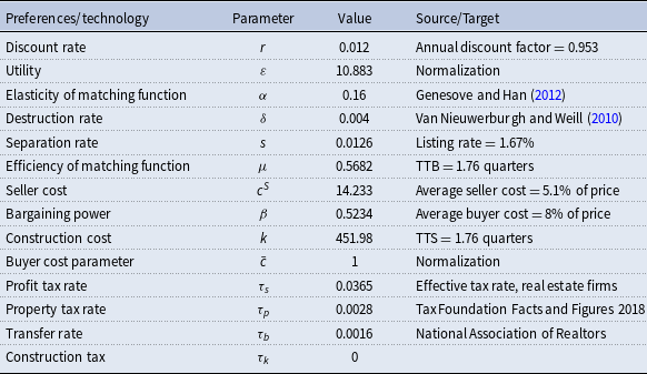
3.2 Calibration

Following Gabrovski and Ortego-Marti (Reference Gabrovski and Ortego-Marti2021a), let $r=0.012$ to match an annual discount factor of $0.953$ . We set $\delta =0.004$ to match an annual housing depreciation rate of $1.6\%$ (Van Nieuwerburgh and Weill, Reference Van Nieuwerburgh and Weill2010). The matching function is assumed to be Cobb-Douglas with $m(\theta ) = \mu \theta ^{-\alpha }$ . The elasticity of the matching function $\alpha$ is equal to $0.16$ , following the empirical evidence in Genesove and Han (Reference Genesove and Han2012). The flow utility of owning a house $\varepsilon$ is normalized to $10.883$ . This implies a steady state price of $491.2$ , which is the average empirically observed price (in thousands of dollars) in Kotova and Zhang (Reference Kotova and Zhang2020). We set a profit tax rate for sellers of $3.65\%$ , which corresponds to the average effective tax rate for the Real Estate Developer firms for the years 2014-2019 as reported by Aswath Damodaran.Footnote ¹⁴ The Tax Foundation in its “Facts and Figures 2018” reports an effective annual property tax rate for the United States of $1.13\%$ . The median real estate transfer tax rate reported by the National Association of Realtors is $0.16\%$ . Following Gabrovski and Ortego-Marti (Reference Gabrovski and Ortego-Marti2019), we assume that $c^B(b) = \bar {c}b^\gamma$ . We normalize $\bar {c}=1$ , which yields $b = 96.29$ .

To obtain the rest of the model parameters we target six moments from the data. The time-to-sell is set to $1.76$ quarters which is the average of the Median Number of Months on Sales Market reported by the U.S. Bureau of Census for the period of 1987:1–2017:4. We also set the time-to-buy to be equal to the time to sell following Gabrovski and Ortego-Marti (Reference Gabrovski and Ortego-Marti2019, Reference Gabrovski and Ortego-Marti2021a) based on the evidence in Genesove and Han (Reference Genesove and Han2012). These two targets yield $\mu =0.5682$ , $k=451.98$ . Ngai and Sheedy (Reference Ngai and Sheedy2020) calculate a listing rate, given by the number of new listings on the market divided by the stock of owner-occupied houses not already for sale, equal to $1.667\%$ . This target implies a separation rate $s=0.0126$ . To calibrate $c^S$ , we target expected costs for the seller equal to $5.1\%$ of the average house price, following Ghent (Reference Ghent2012). Following the same reference we also target an average cost for the buyer of $8\%$ . These two moments yield $c^S = 14.233$ and $\beta = 0.5234$ . Lastly, to calibrate $\gamma$ we use monthly data on vacancies and sales from the New Residential Sales Release reported by the U.S. Bureau of Census for the period January 1963–December 2019.Footnote ¹⁵ Given that in our model sales $=b m(\theta )$ , the information on sales and vacancies allows us to back out a series for the number of buyers using $b = v [\text{sales}/(\mu v)]^{1/(1-\alpha )}$ . Next, we regress the cyclical component of the series for buyers on the cyclical component of the series for vacancies and a constant to arrive at an elasticity of $0.19$ .Footnote ¹⁶ Plugging this estimate into equation (14) in Gabrovski and Ortego-Marti (Reference Gabrovski and Ortego-Marti2019) results in $\gamma =0.68$ . Table 1 summarizes the calibration.

Table 1. Baseline model: calibration

3.3 Results

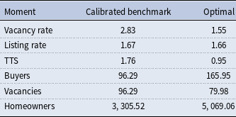
Our calibrated model matches the housing market data well. In particular, vacancy and construction rates, which are not targeted in the calibration, are close to their empirical counterparts. These moments are of particular relevance in our context: the vacancy rate captures liquidity in the housing market, whereas the construction rate captures the importance of the entry channel, which is at the core of our paper. In the model, the vacancy rate is measured as the ratio of vacancies to the total stock of homes and equals $2.83\%$ in the steady state. In the data, the vacancy rate is $1.9\%$ and is measured as the average of the Homeowner Vacancy Rate reported by the United States Census Bureau for the period 1987:1–2017:4. The model also does a relatively good job at matching the construction rate. In the model, this construction rate is measured by the number of homes built divided by the total housing stock, and is equal to $0.4\%$ . In the data, the average of this ratio for the period 1987:1–2017:4 is $0.27\%$ .Footnote ¹⁷

We gauge the distance of the decentralized equilibrium to the planner’s social optimum by focusing on three important measures of liquidity in the housing market: the vacancy rate, the listing rate, and the time-to-sell. The values of these liquidity measures at the steady state equilibrium and at the planner’s optimum are summarized in Table 2. In general, the planner finds it optimal to reduce the relative amount of vacancies in the market and to have houses match with buyers faster. Intuitively, this is due to the congestion externality. In equilibrium sellers extract too much of the surplus which induces an inefficient over-entry into the market. This leads to higher than optimal expected search and construction costs for sellers.

Table 2. Baseline model: moments

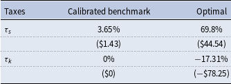
Finally, we quantify the size of the housing policies required to restore efficiency. Table 3 reports the optimal tax rates implied by the model and the dollar amount of these policies, in thousands of dollars. The efficient allocation requires fewer houses for sale and more buyers than the decentralized equilibrium. This can be achieved through a combination of taxes on sellers and a subsidy to housing construction.Footnote ¹⁸ From the HE condition (20), a lower $\tau _k$ and a higher $\tau _s$ both raise the market tightness, which lowers time-to-sell. From the BE condition, the combination of a lower market tightness, a lower $\tau _k$ and a higher $\tau _s$ raises the measure of buyers. Quantitatively, raising the profit tax from $3.65$ to $69.8\%$ and subsidizing construction at a rate $17.31\%$ brings the housing market to its efficient level. In dollar amounts, these policies correspond to $44,540 and $78,250 respectively. To put the dollar amount in perspective, our calibration is such that house prices are $\$491,000$ on average, as in the data.

Table 3. Baseline model: optimal policies