

Introduction
The Intergovernmental Panel on Climate Change (IPCC) Fourth Assessment Report notes that there is considerable uncertainty associated with projected sea-level change over the coming decades and century (Reference SolomonSolomon and others, 2007). Understanding ice-flow dynamics in Greenland and Antarctica is an urgent climate problem; even a modest change in ice-sheet volume will strongly affect future sea level and freshwater flux to the oceans (Reference Lemke and SolomonLemke and others, 2007). However past, present and future ice flow, both by internal deformation and basal sliding, is poorly understood. This uncertainty could be substantially reduced by more and better use of observations of the internal structure of the Greenland and Antarctic ice sheets.
Internal layering is frequently observed in radio-echo soundings (RES) of ice sheets, as well as in smaller polar glaciers. Most internal ice reflectors in these datasets are thought to be isochronous (Reference Bogorodsky, Bentley and GudmandsenBogorodsky and others, 1985). For this reason, the RES architecture provides a picture of the age structure of the ice (Reference EisenEisen, 2008). RES data from both ground- and airborne-based instruments have therefore been used: to investigate changes in ice flow (e.g. Reference SiegertSiegert and others, 2004; Reference Rippin, Siegert, Bamber, Vaughan and CorrRippin and others, 2006); in ice-flow modelling studies (Reference Conway, Hall, Denton, Gades and WaddingtonConway and others, 1999; Reference Siegert, Hindmarsh and HamiltonSiegert and others, 2003; Reference Martín, Hindmarsh and NavarroMartín and others, 2006, Reference Martín, Gudmundsson, Pritchard and Gagliardini2009; Reference Waddington, Neumann, Koutnik, Marshall and MorseWaddington and others, 2007; Reference EisenEisen, 2008); to calculate past accumulation rates (Reference Fahnestock, Abdalati, Luo and GogineniFahnestock and others, 2001); and for the constraint of layer ages from ice cores (Reference Waddington, Neumann, Koutnik, Marshall and MorseWaddington and others, 2007).
Gathering isochronous layer information from RES data traditionally involves picking out and following individual reflectors within RES datasets (e.g. Reference Nereson, Raymond, Jacobel and WaddingtonNereson and others, 2000; Reference Nereson and RaymondNereson and Raymond, 2001; Reference Waddington, Neumann, Koutnik, Marshall and MorseWaddington and others, 2007). This approach requires reflectors with excellent continuity that can be traced for long distances. One application is to use these data in conjunction with ice-flow models that predict isochrones to directly compare model results with tracked layer observations.
A primary consideration in obtaining layer information from RES data is the amount of labour required to carry out the data gathering. We can use hand-picking of bed profiles (e.g. Reference Lythe and VaughanLythe and others, 2001) to calculate how much effort is required to manually pick ice reflectors in RES sections. It took a skilled operative 6 months to hand-pick the bed for 20 000 km of the WISE-ISODYN survey, suggesting that picking 20 internal ice reflectors would take ∼10 years. Thus, while hand-picked continuous isochrones can provide an excellent product, hand-picking of internal ice reflectors at all depths along new extensive RES datasets (these are now available across hundreds of thousands of kilometres of flight-line) is prohibitive in terms of required man-hours. While some largely automated layer-picking techniques have been developed (e.g. Reference Fahnestock, Abdalati, Luo and GogineniFahnestock and others, 2001; Reference Matsuoka, Conway, Catania and RaymondMatsuoka and others, 2009), these still require some operator input.
A second consideration in obtaining layer information is the dependency on continuity. Both manual and auto-picking methods are restricted in applicability to RES datasets with very good reflector continuity. However, Reference Parrenin, Hindmarsh and RémyParrenin and others (2006) and Reference Parrenin and HindmarshParrenin and Hindmarsh (2007) note that identical flow information is contained in the apparent dip of the reflectors. This is useful because dip datasets can be derived from localized reflector information without requiring long-distance continuity. (Note, for brevity we generally use the term ‘dip’ to refer to the ‘apparent dip’ of the isochrones, and if needed, refer to the maximum dip, which is generally not orientated parallel to a survey line, as the ‘true dip’. Throughout this paper, ‘dip’ refers strictly to the tangent of the observed RES reflector slope at a given point.) A constructive proof of the isochrone/dip equivalence is given by Reference Parrenin, Hindmarsh and RémyParrenin and others (2006), who derive an explicit formula for the evolution of dip along a streamline. A more intuitive way to recognize this is to note that isochrones contain no information about horizontal provenance, and are consequently just geometric features that can be equally characterized by their dip. The corollary of this is that continuous apparent dips can also be integrated to provide synthetic isochrones.
Note that, in practice, we require reflector segments of a finite length to measure dip, so the measured dip is not strictly a point measurement. However, by comparison with forward numerical ice-flow models, the spatial averaging of the observed dip datasets generated here is smaller than spatial averaging using typical numerical model grid resolutions. This implies that, in most circumstances, individually hand-picked reflectors or continuous sections of apparent dip can equally well be used.
Since ice-flow models calculate age as a field that depends upon horizontal and vertical position (e.g. Hind-marsh and others, 2009) the modelled slope of the age field at a given elevation in a given horizontal direction can be compared with dip observations. In other words, we can compare observed and modelled dips directly, rather than reconstitute observed dips into isochrones to compare with isochrones outputted from models. Because the measured dips are quantitative data, possibilities of using these data within inverse frameworks also arise. For direct model/ observation comparison or for inverse modelling, there is an issue of how the number of observational data will affect the study, and hence how many dip data may need to be retrieved, which we do not address in this paper. However because the emphasis on continuity of reflectors is substantially reduced by our approach, and the manual effort required is very small, this substantially increases the quantity of usable datasets.
Most glaciologists would argue that good continuous reflectors are better than angle information. By the fundamental theorem of calculus, the two are mathematically equivalent; a dip field can be integrated to give isochrones. In practical terms, very continuous reflectors are associated with very high-quality data, and there is very little difference in practice between automatic picking (which uses the local slope as a predictor) and our method. Our method also works where there is poor continuity, in other words where data quality is worse; in this case our results will also be worse. Of course, with very high-quality data, more data analysis options are available (e.g. stratigraphic correlation), and at this point one has to start considering how precisely radar reflectors map onto isochrones.
Here we present the novel automated finite-segment method to obtain englacial reflector dip angles from either airborne or ground-based RES data. We emphasize that the automated RES processing (ARESP) method is based on measuring local dip: ARESP is not an auto-picking routine, and does not rely on internal reflectors remaining traceable over the whole section. However, the dip datasets produced by ARESP are horizontally integrated here to provide synthetic isochrones, since these are useful to help assess the quality of ARESP dip data. Although this appears similar to a tracked-layer method, these results are produced using an approach quite distinct from an automated version of a tracked-layer method.
To test the ARESP method we apply it to two specific Antarctic RES datasets which appear to be fairly typical of recent ground-based and airborne RES: firstly the 22 km Fletcher Promontory radar line, surveyed using the ground-based Deep-Look Radio Echo Sounder (DELORES), and secondly the 1007 km Wilkes Subglacial Basin (WSB) airborne RES line (see Table 1 for RES dataset characteristics).
Example RES dataset characteristics
Sample Data
RES systems operate by emitting a radar pulse which propagates through the air and the ice sheet. Energy from the pulse is reflected at boundaries between materials of differing dielectric properties and the return signal is recorded. (More details are given by Reference Bogorodsky, Bentley and GudmandsenBogorodsky and others, 1985.)
RES surveys can take place from the air or from the ground. Airborne systems do not always provide the same reflector continuity as the lower-frequency, higher-resolution ground-based systems. The choice of which system to use is severely constrained by logistical considerations as well as the scientific scope of the surveying. Here we demonstrate that, for a tractable ground-based RES dataset, ARESP dips are as good as those derived from hand-picking ice reflectors. For an airborne dataset ARESP again performs convincingly.
Example ground-based data: the Fletcher Promontory
During December 2005 the Fletcher Promontory, West Antarctica, was surveyed using the British Antarctic Survey (BAS) ground-based DELORES radar at 100 MHz, with an effective bandwidth after processing of 5 MHz, and a nominal centre frequency of 4 MHz (Table 1). A trace of 900 returning pulses (sampled at 100 MHz) allows depiction of the full depth of the 600 m thick ice. This dataset has undergone some initial trace stacking and horizontal smoothing prior to the application of our ARESP method. The average resultant horizontal trace resolution is 2.73 m. Figure 1a shows a sample portion of the 22 km Fletcher dataset. For simplicity we present the Figure 1 a RES dataset as localized standard scores, where the standard score is a dimensionless quantity derived by subtracting the local RES dataset population mean from an individual raw score and then dividing the difference by the local population standard deviation. The size of the local population for this conversion spans approximately two ice reflectors in the vertical. (Note, we convert the data only to provide an initial depiction of the dataset; the processing method described hereafter is applied to the raw unconverted data.)
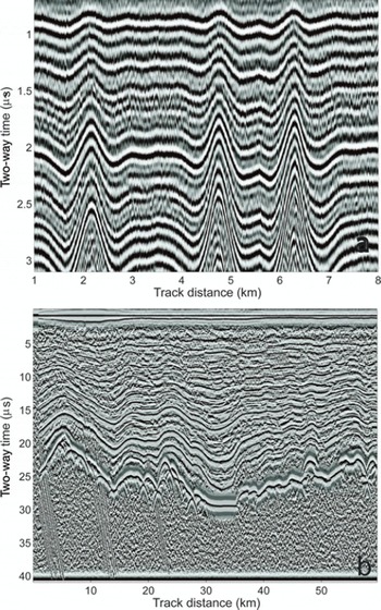
Sample RES sections. (a) 8 km of the ground-based Fletcher Promontory dataset and (b) 59.63 km of the airborne WSB dataset. Both RES datasets are obtained along an approximately straight path. Reflectors are clarified by averaging adjacent traces and converting values to localized standard scores. The shading range for standard scores in each panel is ±2σ.
Example airborne data: the Wilkes Subglacial Basin
During the austral summer of 2005 and 2006 a collaborative UK/Italian project (WISE–ISODYN) conducted an extensive airborne geophysical survey of the Transantarctic Mountains, WSB and the Dome C region (Reference FerraccioliFerraccioli and others, 2007). We use a 1007 km long flight-line from this dataset (for brevity, hereafter referred to as the WSB data).
For the WSB data (Table 1), a trace of 1400 returns is sampled at 22 MHz, with an effective bandwidth after processing of 5 MHz and a nominal centre frequency of 150 MHz (Reference CorrCorr and others, 2007). Twenty-five of these samples are stacked to record the trace returns at 312.5 Hz, roughly every 0.2 m, at the given WSB flight speed, along the flight path. This yields a total recorded WSB dataset size of 47 GB. During the initial recording and pre-processing stage, the received pulses are fed through a high-gain chirp channel where the chirp is compressed. This airborne example, unlike the ground-based example above, has therefore not had any initial pre-processing applied, apart from the stacking and on-board processing that occurs during the initial echo recording.
Figure 1b shows a 59.63 km sample section of the total 1007 km long WSB dataset; the sample section starts at 72.85° S, 159.04° E, ends at 73.03° S, 157.31° E and is formed of ∼300 000 traces, with a horizontal trace separation (Δx1) of ∼0.2 m. Note the data shown have been converted to localized standard scores to enable this initial visualization of the reflectors (it does not represent ‘raw’ data). The WSB ice thickness in the first 60 km of section varies between ∼2.1 and 3.3 km. Figure 1b therefore shows the echo returns recorded down to 42 s, or ∼3.5 km, in depth (as standard scores). Reflectors can be detected throughout most of the dataset, with the exception of the upper few hundred metres and the few hundred metres closest to the bed.
Processing Method
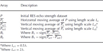
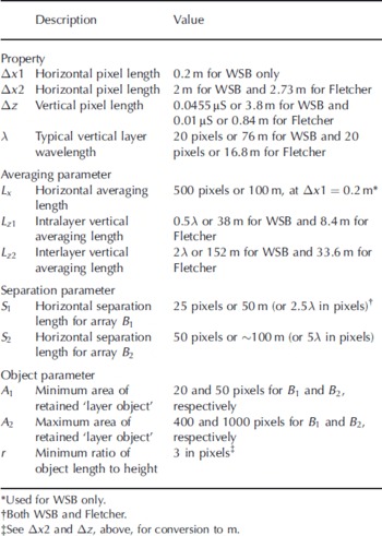
Here we outline the fully automated processing method (Fig. 2) which we apply to the initial echo return strength datasets (herein these RES datasets are referred to as P). In summary the steps are: (1) reduce RES inter-trace noise by horizontal averaging; (2) obtain binary dataset by local thresholding; (3a) identify short coherent layer segments, or ‘layer objects’, by horizontal discretization of the binary data; (3b) measure layer object properties; (3c) discard invalid layer objects; and (3d) collate the non-uniformly distributed object dip information. Note we use layers here to refer to reflectors with a finite thickness. Table 2 shows the two-dimensional arrays used during the processing, and Table 3 the RES data properties and ARESP parameters used.
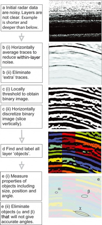
Schematic description of processing method. Panels are illustrative, and are horizontally compressed to make the description clearer. (a) Unprocessed data on a logarithmic greyscale. (b–e) Horizontally compressed data: (b) noise-reduced data (logarithmic greyscale); (c) converted to binary; (d) horizontally sectioned with individual ‘layer objects’ coloured to indicate separate entities; (e) examples of ‘layer objects’. α and β are too small and/or equiaxial so are excluded, whereas χ is a valid ‘layer object’. Its orientation information is retained.
Arrays generated and used during ARESP
Properties of RES data and ARESP parameters
Step 1: noise reduction
Initial processing is designed simply to reduce inter-trace noise. Adjacent traces (Δx1= 0.2 m apart) in the P WSB can feature echo amplitudes which are an order of magnitude different. The correlation between adjacent traces is also quite low (typically R = 0.80 for traces ∼5 m apart). Since the RES ice layers tend to show a strong degree of horizontal persistence, it is possible to enhance the signal-to-noise ratio by simple horizontal averaging.
Firstly, a moving average of length scale Lx
= 500 adjacent traces at a time (∼100 m of radar section) is performed to increase the signal-to-noise ratio. Initial investigations of the RES data (during trial runs of ARESP) indicate that layer slopes do not tend to exceed 30% in our test datasets. Therefore, averaging 50 m on either side ensures that generally we are averaging within, rather than through, dipping layers. This yields long lengths of continuous radar layer. Secondly, the horizontal resolution is reduced by a factor of 10, to account for the subsequent ‘oversampling’ induced by the horizontal averaging, to leave a horizontal resolution Δx2 = 2 m, i.e. one trace every 2 m. This stage produces an initial horizontally averaged ‘noise-reduced’ version of P, which we term ![]() . The horizontal pixel length, Δx
2, of 2 m also roughly corresponds to the average trace distance of 2.73 m for the Fletcher RES dataset.
. The horizontal pixel length, Δx
2, of 2 m also roughly corresponds to the average trace distance of 2.73 m for the Fletcher RES dataset.
Additionally, a version of P with vertical averaging, to further reduce noise, is calculated. This is done by applying a vertical moving mean, with a length scale of half of a typical vertical layer wavelength (i.e. averaging length scale Lz
1 = 0.5λ), to ![]() to produce
to produce ![]() This yields an array the same size as
This yields an array the same size as ![]() , in which layers that are less than ∼38 m thick for WSB (8 m for Fletcher Promontory) are smoothed out.
, in which layers that are less than ∼38 m thick for WSB (8 m for Fletcher Promontory) are smoothed out.
Because the ground-based example RES dataset had undergone horizontal averaging prior to our obtaining the dataset, we did not need to apply this initial horizontal averaging ‘noise reduction’ step to obtain ![]() for the Fletcher Promontory data:
for the Fletcher Promontory data: ![]() is effectively the P
Fletcher initial dataset. However, all other steps, including the second noise reduction stage (to obtain
is effectively the P
Fletcher initial dataset. However, all other steps, including the second noise reduction stage (to obtain ![]() ), are applied identically to obtain both our ground-based and airborne test RES datasets.
), are applied identically to obtain both our ground-based and airborne test RES datasets.
Step 2: obtaining a binary layer dataset
Approaches to thresholding
There are two main approaches to identifying layer boundaries using noise-reduced P: either simply thresholding the original data, or thresholding a first- or second-derivative product. During the thresholding process, individual RES values are marked as ‘layer’ pixels if their value is greater than the defined threshold value (assuming a layer to be higher value than the local background) and otherwise as ‘not layer’ pixels. The simple thresholding works on the assumption that layers with low returns represent gaps between more reflective layers. The alternative approach, of thresholding dataset derivatives, works on the assumption that the zones of most rapid change in intensity occur between layers. Sophisticated second-derivative methods, such as the Canny approach (Reference CannyCanny, 1986), take this a stage further and compute the local maximum of the gradient of image intensity. These derivative methods can have the advantage of defining edges only a single value deep and/or wide, so they may be the best option in situations with strong layer edge definition, though they can be sensitive to noise (e.g. Reference Sime and FergusonSime and Ferguson, 2003).
Initial tests (not shown) suggest that first- and second-derivative products are rather sensitive to RES noise, and are unreliable for airborne RES data, even after the noise-reduction processing (step 1). As such, they are not explored further here, but it may be of interest to examine derivative methods further when considering possible future radar layer processing developments. A robust means to automatically find layers is through the production of binary ‘layer or not layer’ data by directly thresholding the ![]() and
and ![]() arrays.
arrays.
Thresholding using a localized threshold
The noise-reduced ![]() and
and ![]() arrays still have regional contrasts in intensity, and a large reduction in echo strength with depth. A localized threshold value helps to correct for these regional differences. A threshold array, the same size as the noise-reduced data array, is calculated. This is done by applying a longer length scale vertical moving mean. The length scale used is twice the typical vertical layer wavelength (i.e. averaging length scale Lz
2 = 2λ), to
arrays still have regional contrasts in intensity, and a large reduction in echo strength with depth. A localized threshold value helps to correct for these regional differences. A threshold array, the same size as the noise-reduced data array, is calculated. This is done by applying a longer length scale vertical moving mean. The length scale used is twice the typical vertical layer wavelength (i.e. averaging length scale Lz
2 = 2λ), to ![]() to obtain
to obtain ![]() . The array
. The array ![]() has all individual reflectors smoothed out, but it retains regional changes (i.e. over tens to hundreds of metres) in P.
has all individual reflectors smoothed out, but it retains regional changes (i.e. over tens to hundreds of metres) in P.
Binary datasets are obtained by subtracting the threshold array, ![]() , from
, from ![]() and
and ![]() and retaining the sign of the resultant array, i.e. the binary dataset
and retaining the sign of the resultant array, i.e. the binary dataset ![]() and a second binary dataset, with reduced intralayer noise,
and a second binary dataset, with reduced intralayer noise, ![]() . Note ‘sign’ means any value above zero is classified as ‘layer’, and any value below zero is classified as ‘not layer’ (e.g. Fig. 2c). By definition, thresholding using
. Note ‘sign’ means any value above zero is classified as ‘layer’, and any value below zero is classified as ‘not layer’ (e.g. Fig. 2c). By definition, thresholding using ![]() ensures that the binary datasets, B
1 and B
2, are both ∼50% reflective ‘layer’ (logically positive) and 50% unreflective ‘not layer’ (logically negative).
ensures that the binary datasets, B
1 and B
2, are both ∼50% reflective ‘layer’ (logically positive) and 50% unreflective ‘not layer’ (logically negative).
Whilst using the two separate B 1 and B 2 arrays is not essential, it does provide a more robust characterization of layer dips, because the arrays identify layers of different thicknesses. For some regions, B 1 reliably identifies thinner layers, whilst for other, noisy, regions B 2 provides more reliable identification for thicker layers. Throughout steps a to 3c the binary layer datasets, B 1 and B 2, are processed separately. Then all the dips measured from both B 1 and B 2 are collated during step 6 to provide a thorough survey of the radar layer angles.
Step 3: obtaining layer dips
Calculating the binary datasets, B 1 and B 2, while bringing out the ice layers, does not quantify the dip angle information. We still need to measure these dip values.
Step 3a: isolating ‘layer objects’
The next stage of the automated processing is to extract dip information. This stage is begun by horizontally separating the binary arrays into thin vertical strips. ‘Layer objects’ are isolated using a horizontal separation length, S 1, of 25 horizontal pixels (∼50 m) for B 1 and a separation length, S 2, of 50 pixels (∼100 m), for the two binary arrays (e.g. Fig. 2d). An ‘object’ in this sense is a selection of values adjacent to each other, within the same strip, which are all of the same logical value, i.e. which comprise a short horizontal strip of identifiable radar layer. The binary arrays are also inverted so that ‘layer objects’ are identified also using the low, as well as high, reflectivity as a criterion (not illustrated in Fig. 2). To maximize the number of ‘layer objects’ identified, B 1 and B 2 can also be sampled in overlapping strips.
Step 3b: measuring ‘layer objects’
Once ‘layer objects’ are identified (as individual selections of adjacent values with the same logical property), by horizontally separating the objects in discrete strips (step 3a), the properties of the individual objects are measured. Morphological measurements are made of the object position, area, major axis length, minor axis length and orientation (Fig. 2e). Object area, major axis length and minor axis length are used to assess whether the object is likely to give accurate layer orientation information, i.e. whether it is a valid ‘layer object’ or ‘noise’, whilst object position is needed to locate each valid layer object.
Step 3c: eliminating invalid ‘layer objects’
Several criteria are used to find layer ‘noise’, i.e. measured objects which would provide erroneous layer dip data (see Table 3). Firstly, any object that is too small to be reliable as a layer object is removed from the analysis. The pixel area, A 1, is used as the criterion for removal; some examples can be seen in Figure 2e. Secondly, any object with an area that is too large, where it may comprise several ‘true’ layers, is likely to provide inaccurate dip information. Here pixel area, A 2, is used as the criterion for removal. Thirdly, any object possessing a pixel aspect ratio, r, of <3:1 is eliminated, since approximately equiaxial objects do not provide reliable dip estimates. The remainder of the layer object information is retained.
Step 3d: collating ‘layer object’ angle data
Finally, the object dip information is collated by location. The automatically measured ‘layer objects’ are not distributed uniformly across the radar section. A gridded dip dataset is formed by taking the median of local sets of dip estimates (gridded results are shown in Figs 3a and 4a). Tests (not shown) indicate that the sample size used for this gridding procedure does not have a strong impact on these results, provided the number is kept high enough to provide a statistically robust sample (for our sample datasets this is ∼80). Note that Figure 2d and e illustrate dip measurements being made on a horizontally compressed version of the binary data. The example section shown in Figure 2d and e is ∼4 km long, so the ARESP processing method in reality samples ∼1200 objects per layer across this section of data, rather than the illustrative four objects per layer shown in Figure 2d.
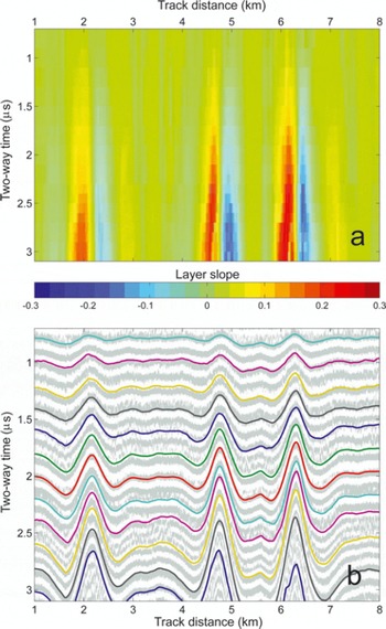
Fletcher Promontory example ground-based RES section. (a) The collated ARESP layer slope data and (b) B 2 grey image overlaid with synthetic isochrone ‘layers’ projected from the layer dip data.
Results
Example sections from the ground-based Fletcher Promontory and WSB airborne RES datasets are shown in Figures 3 and 4, respectively. Upper panels illustrate the collated gridded ARESP ice layer dip data, whilst lowest panels show some ‘synthetic isochrones’ projected from the ARESP dip data, over binary B 2 arrays. For the ground-based Fletcher dataset, visual inspection of Figure 3b indicates that ARESP results are as good as those which would be obtained from hand-picking layers.
The large set of automatically detected and measured ‘layer objects’ enables errors associated with the automatic detection method, and with RES data noise, to be quantified. For example, Figure 4b shows the standard deviation associated with local sets of dip observations. High values show that the ‘layer objects’ measured are quite variable in dip; the collated ‘layer object’ dip data (Fig. 4a) are uncertain in these regions. The near-surface and near-bed regions stand out as having uncertain ice layer dips.
WSB example airborne RES section. (a) Collated ARESP layer slope data, (b) standard deviation associated with the ARESP slope data and (c) the WSB B 2 grey image overlaid with synthetic isochrone ‘layers’ projected from the layer dip data.
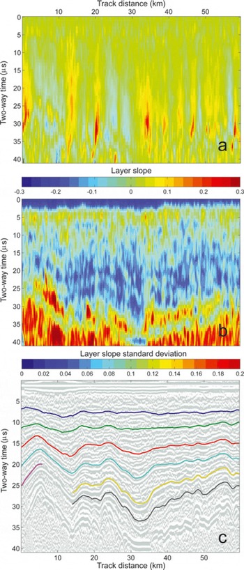
Inspection of Figure 4c suggests that some RES reflectors in the airborne dataset may be discontinuous. The standard deviation (Fig. 4b) confirms that, whilst reflectors can be detected throughout most of the dataset, the upper few hundred metres and the few hundred metres closest to the bed do not have reliably detectable coherent ice reflectors. Additionally, some high-angle radar artefact layers are visible in near-bed regions associated with high bed dips (within the first 20 km of the flight-line). Together these cause a near-bed region, at ∼24–33 μS in depth and 4–12 km track distance, where the ice reflector dips cannot be accurately ascertained (red region above the bed in Fig. 4b). In consequence, we do not attempt to project layers (synthetic isochrones) over this region, since ARESP cannot provide reliable dip angles in this region. For regions where RES ice reflectors are more coherent, the Figure 4c airborne RES projected line results are comparable to those which would be obtained from hand-picking methods.
Conclusion
The novel automated method presented here is robust: identical ARESP using identical parameter values function equally well on recent airborne and ground-based RES datasets, without the need for any ARESP parameter tuning. Additional tests indicate that ARESP, as presented here, performs equally well on alternative ground-based and airborne datasets (not shown). However, we note that minor changes in the ARESP parameter values, such as in the noise reduction (Lx and L z1 and L z2 averaging lengths), and the criteria used to eliminate invalid ‘layer objects’ (i.e. A 1 and A 2), are likely to be required to optimize ARESP for differing RES datasets. Automating the specification of A, and setting the ARESP parameters to be functions of A, may enable future ARESP developments to minimize any dataset-specific parameterization changes.
In terms of processing time required, on a modest desktop computer (3 GHz clock speed, with 3 GB RAM), the WSB dataset (1007 km in length and 47 GB in size) was processed in around 10 wall-clock hours and the 22 km Fletcher example took a few minutes. This implies that on this set-up, 1 TB (or ∼20 000 km) of airborne data can be processed in less than a week. Setting up the ARESP algorithms in a high-performance multi-processor environment and/or using higher-speed disks could enable faster processing of RES data.
While hand-picked continuous isochrones are a very good product, hand-picking large RES datasets for lots of ice reflectors is not generally feasible in terms of the manual effort required; applying ARESP to the >100 000 km of airborne line surveys of East Antarctica can potentially save more than half a century of manual labour.
As well as the time-saving advantage, the ARESP method has other possible advantages over the manual hand-picking method. Firstly, because ARESP uses only local reflector dip information, continuous reflectors along the whole length of the RES section are not necessary to allow collation of ARESP dip datasets. Secondly, the relatively complete ARESP measurement of local ice reflector dips can allow a thorough characterization of dip angle uncertainty. These advantages may allow ARESP to help with ice-flow model/data comparison studies and with inverse model studies.
In conclusion, the efficiently processed dip angle datasets produced by the ARESP method should substantially help glaciologists seeking to understand ice-flow dynamics in Greenland and Antarctica. ARESP has the potential to change the way we model isochrones; it could enable glaciologists to move from selective case studies to large-scale studies using all the available RES ice reflector data.
Acknowledgements
We thank K. Matsuoka and an anonymous reviewer for insightful reviews which improved the manuscript. This study is part of the BAS Polar Science for Planet Earth Programme. It was funded by the UK Natural Environment Research Council.


