


1. Introduction
Climate change impacts the water cycle and the cryosphere across major global regions, with regional-specific responses such as increasing frequency and intensity of extreme precipitation events, accelerated glacier melt, and more intense and/or longer droughts (Allan et al., Reference Allan, Barlow, Byrne, Cherchi, Douville, Fowler, Gan, Pendergrass, Rosenfeld, Swann, Wilcox and Zolina2020; Hugonnet et al., Reference Hugonnet, McNabb, Berthier, Menounos, Nuth, Girod, Farinotti, Huss, Dussaillant, Brun and Kääb2021; IPCC, Reference Masson-Delmotte, Zhai, Pirani, Connors, Péan, Berger, Caud, Chen, Goldfarb, Gomis, Huang, Leitzell, Lonnoy, Matthews, Maycock, Waterfield, Yelekçi, Yu and Zhou2021). Although climate change significantly affects water availability, recent studies have found that human water use, due to technological and demand-side characteristics, is the main driver of water scarcity across different future scenarios (Graham et al., Reference Graham, Hejazi, Chen, Davies, Edmonds, Kim, Turner, Li, Vernon, Calvin, Miralles-Wilhelm, Clarke, Kyle, Link, Patel, Snyder and Wise2020; Hanasaki et al., Reference Hanasaki, Fujimori, Yamamoto, Yoshikawa, Masaki, Hijioka, Kainuma, Kanamori, Masui, Takahashi and Kanae2013; Satoh et al., Reference Satoh, Kahil, Byers, Burek, Fischer, Tramberend, Greve, Flörke, Eisner, Hanasaki, Magnuszewski, Nava, Cosgrove, Langan and Wada2017).
Based on different approaches to measure water scarcity, some regions of the world have been consistently identified as present or future water scarcity hotspots (Leijnse et al., Reference Leijnse, Bierkens, Gommans, Lin, Tait and Wanders2024). Some of these hotspots depend on meltwater from snow or glaciers to provide water resources, especially for irrigation during the driest months of the year. Among these hotspots, we find South and Central Asian basins like the Indus and Amu Darya, or countries like Kazakhstan, Uzbekistan, Pakistan, Afghanistan, and Northern India (Bijl et al., Reference Bijl, Biemans, Bogaart, Dekker, Doelman, Stehfest and van Vuuren2018; Du et al., Reference Du, Xu and Li2021; Hanasaki et al., Reference Hanasaki, Fujimori, Yamamoto, Yoshikawa, Masaki, Hijioka, Kainuma, Kanamori, Masui, Takahashi and Kanae2013; Huang et al., Reference Huang, Yuan and Liu2021; Liu et al., Reference Liu, Liu, Yang, Ciais and Wada2022; Satoh et al., Reference Satoh, Kahil, Byers, Burek, Fischer, Tramberend, Greve, Flörke, Eisner, Hanasaki, Magnuszewski, Nava, Cosgrove, Langan and Wada2017). In the Andean region, North-Central Chile and Northwest Argentina have been identified as present or future water scarcity hotspots under climate change scenarios (Hanasaki et al., Reference Hanasaki, Fujimori, Yamamoto, Yoshikawa, Masaki, Hijioka, Kainuma, Kanamori, Masui, Takahashi and Kanae2013; Huang et al., Reference Huang, Yuan and Liu2021; Liu et al., Reference Liu, Liu, Yang, Ciais and Wada2022).
Recent studies have highlighted that the maximum contribution of glaciers to runoff has either been reached in recent years or is projected to occur in the coming decades of the 21st century due to the rapid glacier mass loss observed and anticipated under current climate change scenarios (Bliss et al., Reference Bliss, Hock and Radić2014; Caro et al., Reference Caro, Condom, Rabatel, Champollion, García and Saavedra2024; Huss & Hock, Reference Huss and Hock2018; Moore et al., Reference Moore, Pelto, Menounos and Hutchinson2020; Wimberly et al., Reference Wimberly, Ultee, Schuster, Huss, Rounce, Maussion, Coats, Mackay and Holmgren2025). After the peak in glacier runoff, the contribution of glaciers to runoff declines, falling below their historical contribution (Bliss et al., Reference Bliss, Hock and Radić2014; Caro et al., Reference Caro, Condom, Rabatel, Champollion, García and Saavedra2024; Huss & Hock, Reference Huss and Hock2018). Given the importance of glacier runoff in supporting water availability during the dry season, a reduction in glacier runoff following the peak water glacier runoff can impact water scarcity in highly glacierized basins (Biemans et al., Reference Biemans, Siderius, Lutz, Nepal, Ahmad, Hassan, von Bloh, Wijngaard, Wester, Shrestha and Immerzeel2019; Caro et al., Reference Caro, Condom, Rabatel, Champollion, García and Saavedra2024; Lutz et al., Reference Lutz, Immerzeel, Siderius, Wijngaard, Nepal, Shrestha, Wester and Biemans2022).
Previous studies have estimated future water scarcity using the Shared Socioeconomic Pathways (SSP) socioeconomic assumptions and Representative Concentration Pathways (RCP) hydro-climatic conditions (e.g., Hanasaki et al., Reference Hanasaki, Fujimori, Yamamoto, Yoshikawa, Masaki, Hijioka, Kainuma, Kanamori, Masui, Takahashi and Kanae2013; Liu et al., Reference Liu, Liu, Yang, Ciais and Wada2022). However, most of them have not included the response of economic systems (agricultural, energy) to changes in water availability in their modeling approach and instead maintain predefined water use trajectories based on SSP socioeconomic assumptions.
In addition, although meltwater plays a relevant role in the above-mentioned hotspots, most of the previous literature has not explicitly modeled glacier runoff to assess future water scarcity conditions considering peak water glacier runoff and changes in glacier contribution to runoff. Various Global Hydrological Models (GHM) used in previous assessments (e.g., H08, WaterGAP, and LPJML) do not include a separate glacier model that can distinguish between glacier runoff and snowmelt and incorporate changes in glacier area and volume.
In this study, we estimate water scarcity conditions in glacierized basins of Asia and the Andes under three SSP scenarios (SSP1-2.6, SSP3-7.0, and SSP5-8.5) combining water availability estimations from the Open Global Glacier Model (OGGM) and the Xanthos framework (Li et al., Reference Li, Vernon, Hejazi, Link, Feng, Liu and Rauchenstein2017; Maussion et al., Reference Maussion, Butenko, Champollion, Dusch, Eis, Fourteau, Gregor, Jarosch, Landmann, Oesterle, Recinos, Rothenpieler, Vlug, Wild and Marzeion2019) and water demand (WD) estimations using the Global Change Analysis Model (GCAM). This work improves previous estimations in two ways. First, we force an Integrated Assessment Model (GCAM) (JGCRI, 2023) with varying water availability under the selected climate change scenarios to include the economic response of the agricultural sector (via blue water availability for irrigation). Second, we link a glacier (OGGM) and a hydrological model (Xanthos) to explicitly include the changes in glacier runoff in water scarcity assessment.
2. Data and methods
The methods used in this research follow three phases described in detail in the next subsections and are summarized in Figure 1. First, we estimate water availability under three different SSP scenarios with our own modified version of the GHM Xanthos, which now includes glacier runoff as a runoff source using the output of the OGGM (Li et al., Reference Li, Vernon, Hejazi, Link, Feng, Liu and Rauchenstein2017; Maussion et al., Reference Maussion, Butenko, Champollion, Dusch, Eis, Fourteau, Gregor, Jarosch, Landmann, Oesterle, Recinos, Rothenpieler, Vlug, Wild and Marzeion2019; Vernon et al., Reference Vernon, Hejazi, Turner, Liu, Braun, Li and Link2019). We use three scenarios from the SSP framework (SSP1-2.6, SSP3-7.0, and SSP5-8.5) – combining a socioeconomic trajectory with a consistent forcing scenario (O'Neill et al., Reference O'Neill, Tebaldi, Van Vuuren, Eyring, Friedlingstein, Hurtt, Knutti, Kriegler, Lamarque, Lowe, Meehl, Moss, Riahi and Sanderson2016; Riahi et al., Reference Riahi, van Vuuren, Kriegler, Edmonds, O'Neill, Fujimori, Bauer, Calvin, Dellink, Fricko, Lutz, Popp, Cuaresma, Kc, Leimbach, Jiang, Kram, Rao, Emmerling and Tavoni2017) – that are present in the Inter-Sectorial Impact Model Intercomparison Project in its version 3b – ISIMIP3b (Frieler et al., Reference Frieler, Volkholz, Lange, Schewe, Mengel, Del Rocío Rivas López, Otto, Reyer, Karger, Malle, Treu, Menz, Blanchard, Harrison, Petrik, Eddy, Ortega-Cisneros, Novaglio, Rousseau and Bechtold2024). The Inter-Sectoral Impact Model Intercomparison Project (ISIMIP) is a scientific effort powered by the Potsdam Institute for Climate Impact Research to create and provide coordination, protocols, and openly available datasets to conduct climate change impact assessments (Frieler et al., Reference Frieler, Volkholz, Lange, Schewe, Mengel, Del Rocío Rivas López, Otto, Reyer, Karger, Malle, Treu, Menz, Blanchard, Harrison, Petrik, Eddy, Ortega-Cisneros, Novaglio, Rousseau and Bechtold2024).
Integrated assessment modeling schema. Purple boxes correspond to exogenous databases and parameters. Dashed blue boxes correspond to models or modules within a model used here. Solid blue boxes correspond to outputs from each model.

Second, we use the Integrated Assessment Model GCAM to project WD under the same SSP scenarios using the estimation of available water of OGGM-Xanthos simulation as one of its inputs. Third, to improve the spatial resolution of our analysis in some basins, we downscale water and land use from GCAM results to a 0.5° grid using Demeter and Tethys and estimate monthly water balance at the basin scale.
In the case of OGGM, Xanthos, and GCAM, we use the default GCAM basins that include Amu Darya, Indus, and Tarim Interior in the case of Asia, and South America Colorado and North Chile Pacific Coast in the case of Andean basins (see Figure 2). However, given that in the Andes, water requirements, land use, and glaciers are concentrated in some subbasins, we estimate water balance in two subbasins of Chile Coastal basins (Aconcagua-Choapa and Maipo basins – see Figure 2) using the downscaled outputs of GCAM using tools like Demeter for land use and Tethys for WD (see Sections 2.3 and 2.4 for details).
Selected basins in this study. Orange polygons represent the subbasins used with the downscaled results using Demeter and Tethys.

2.1. OGGM and xanthos simulations
To estimate glacier runoff, defined here as the amount of ice and snowmelt originating from the glacier area, we used the default monthly temperature-index model within the OGGM version 1.6.1. (Maussion et al., Reference Maussion, Butenko, Champollion, Dusch, Eis, Fourteau, Gregor, Jarosch, Landmann, Oesterle, Recinos, Rothenpieler, Vlug, Wild and Marzeion2019), a global glacier model designed to reproduce and project glacier dynamics and mass balance. We used the default calibration parameters included within the OGGM v1.6.1 that arise from a calibration procedure using the global geodetic mass balance developed by Hugonnet et al. (Reference Hugonnet, McNabb, Berthier, Menounos, Nuth, Girod, Farinotti, Huss, Dussaillant, Brun and Kääb2021) and the GSWP3-W5E5 climate dataset for the period 2000–2020. The OGGM model calibrates three parameters to match the abovementioned geodetic mass balance observations: the melt factor represents the temperature sensitivity of the glacier, the precipitation factor is a scaling factor of the precipitation data, and the temperature bias is a correction to the temperature data. The average melt factor parameter of our set of glaciers is 6.29 kg water equivalent per day (minimum = 1.4, maximum = 17.775). On the other hand, the average precipitation factor average is 4.69 (minimum = 1.65, maximum = 9.74), and the average temperature bias is −3.39 (minimum = −13.27, maximum = 11.74).
We used the Randolph Glacier Inventory version 6.2 (RGI Consortium, 2017) within the selected basins to identify the mountain glaciers to model with OGGM, excluding marine-terminating glaciers. We also excluded a small portion of glaciers, representing 0.18% of the glacier area within the studied basins (115.59 km2), for which successful calibration with OGGM was not feasible (see Table S1 in the Supplementary Material). Regarding ice thickness, we rely on the default OGGM calibration, which calibrates its ice thickness estimation in reference to the global consensus estimate by Farinotti et al. (Reference Farinotti, Huss, Fürst, Landmann, Machguth, Maussion and Pandit2019).
To estimate basin runoff and accessible water, we used a modified version of the Xanthos global hydrological framework which can estimate monthly basin runoff and accessible water at 0.5° resolution (Li et al., Reference Li, Vernon, Hejazi, Link, Feng, Liu and Rauchenstein2017; Vernon et al., Reference Vernon, Hejazi, Turner, Liu, Braun, Li and Link2019). Accessible water is defined in Xanthos (and used as input in GCAM) as the amount of annual basin runoff that is technically and biophysically accessible, considering storage (dams, reservoirs) and seasonal availability (Li et al., Reference Li, Vernon, Hejazi, Link, Feng, Liu and Rauchenstein2017; Vernon et al., Reference Vernon, Hejazi, Turner, Liu, Braun, Li and Link2019).
In Xanthos, we use the ABCDM conceptual model that calibrates five parameters (a, b, c, d, and m): a, which relates to the amount of runoff that occurs when soil is undersaturated; b, which represents the saturation level of the soil; c, which relates to the groundwater recharge capacity of the basin; d, which represents the groundwater discharge; and m, which relates to the fraction of snowpack that is available to melt (Li et al., Reference Li, Vernon, Hejazi, Link, Feng, Liu and Rauchenstein2017; Liu et al., Reference Liu, Hejazi, Li, Zhang and Leng2018; Vernon et al., Reference Vernon, Hejazi, Turner, Liu, Braun, Li and Link2019).
We calibrated the five ABCDM parameters using the default differential evolution optimization algorithm included in Xanthos under the GSWP3-W5E5 climate between 1971 and 2019 using the G-RUN multimodel mean runoff as observations (Cucchi et al., Reference Cucchi, Weedon, Amici, Bellouin, Lange, Müller Schmied, Hersbach and Buontempo2020; Ghiggi et al., Reference Ghiggi, Humphrey, Seneviratne and Gudmundsson2021; Lange et al., Reference Lange, Menz, Gleixner, Cucchi, Weedon, Amici, Bellouin, Schmied, Buontempo and Cagnazzo2021; Vernon et al., Reference Vernon, Hejazi, Turner, Liu, Braun, Li and Link2019). G-RUN is an observation-based global runoff reanalysis that reconstructs basin runoff between 1901 and 2019 using a Random Forest model fitted on runoff observational datasets (Ghiggi et al., Reference Ghiggi, Humphrey, Seneviratne and Gudmundsson2021). After calibration, our simulation performed well for all selected basins, reaching Kling Gupta Efficiency (KGE) values over 0.8 for the North Chile Pacific Coast, Amu Darya, and Indus Basin. In the cases of South America Colorado and Tarim Interior basin, KGE is 0.63 and 0.79, respectively (see Table S2 and Figure S1 in the Supplementary Material).
This work modified the ABCDM model to estimate the water inputs as the sum of precipitation, soil moisture of the previous time step, snowmelt, and glacier runoff. While previously, it only considered precipitation, soil moisture, and snowmelt. As mentioned above, glacier runoff is defined here as the amount of ice and snowmelt originating from the varying glacier area.
To include glacier runoff from OGGM estimates into Xanthos procedures, we transform the outputs from OGGM from the glacier level to a 0.5° gridded dataset using the RGI latitude and longitude data of the glacier terminus. In this way, we assume that the runoff contribution of a glacier flows from its terminus to the basin. Hence, the total glacier runoff within a given grid is computed as the sum of the runoff contributions from all glaciers whose termini are located within that grid.
Hanus et al. (Reference Hanus, Schuster, Burek, Maussion, Wada and Viviroli2024) coupled OGGM with another GHM and implemented a more complex grid transformation considering the percentage of glacier area within grids (Hanus et al., Reference Hanus, Schuster, Burek, Maussion, Wada and Viviroli2024). Wiersma et al. (Reference Wiersma, Aerts, Zekollari, Hrachowitz, Drost, Huss, Sutanudjaja and Hut2022), on the other hand, resampled the individual glacier data to the GHM spatial resolution (5 arcmin) (Wiersma et al., Reference Wiersma, Aerts, Zekollari, Hrachowitz, Drost, Huss, Sutanudjaja and Hut2022). We argue that the simplified coupling method used in this work is appropriate for our coarser spatial resolution (0.5°), where sub-grid spatial variability in glacier extent and runoff pathways has a minor influence on large-scale discharge patterns. At such coarser scales, the hydrological signal represents an aggregated response, and the potential bias from not redistributing glacier runoff across multiple grid cells is less significant relative to other large-scale uncertainties. Our modeling framework may result in partial double-counting of snowfall over glacierized areas, as snowfall is included both as input to OGGM and to the Xanthos hydrological model. The calibration of the M parameter in the ABCDM model reduces this issue by adjusting the effective amount of snow available for melt in the hydrological component. Nevertheless, this calibration does not fully eliminate the double-counting, which may lead to an overestimation of the snowmelt component of glacier runoff (i.e., the seasonal snowfall that melts over glacier surfaces and is also represented in OGGM). This methodological limitation should be addressed in future work through a more integrated treatment of snowfall inputs between OGGM and Xanthos. On the other hand, because glacier runoff is defined exclusively as snow- and ice-melt over glacier areas, liquid precipitation is excluded from OGGM outputs, thereby avoiding double-counting of rainfall inputs.
We run a set of OGGM and Xanthos simulations under SSP1-2.6, SSP3-7.0, and SSP5-8.5 using the temperature and precipitation of the 5 bias-corrected and downscaled Global Circulation Model part of ISIMIP3b design (GFDL-ESM4, IPSL-CM6A-LR, MPI-ESM1-2-HR, MRI-ESM2-0, and UKESM1-0-LL) (Lange, Reference Lange2019).
2.2. GCAM integrated assessment model
GCAM represents the global economy, based on 32 geoeconomics regions, through a recursive general equilibrium model with a 5-year timestep that requires input assumptions about population growth, labor productivity, and economic growth (JGCRI, 2023).
Using exogenous water supply estimations for 235 basins (from OGGM-Xanthos estimations in our case), GCAM estimates WD for six consumption sectors: Agriculture, Livestock, Manufacturing, Municipal, Electricity generation, and Mining (primary energy extraction) (JGCRI, 2023). If the surface available water (SAW) is reduced, the model reacts by increasing water desalination and the depth of groundwater extraction; both alternatives have an associated cost that could impact agricultural production (Kim et al., Reference Kim, Hejazi, Liu, Calvin, Clarke, Edmonds, Kyle, Patel, Wise and Davies2016).
WD in GCAM is estimated using sector-specific coefficients and assumptions. For the Electricity sector, GCAM uses water withdrawal coefficients for each cooling technology in thermo-electric power generation (Hejazi et al., Reference Hejazi, Edmonds, Clarke, Kyle, Davies, Chaturvedi, Wise, Patel, Eom, Calvin, Moss and Kim2014). The choice and availability of these cooling technologies depend on regional characteristics, and technology adoption is endogenously estimated in GCAM based on the cost of each alternative (JGCRI, 2023). In the Mining (oil, coal, and gas extraction) and Manufacturing sectors, GCAM uses coefficients that scale base year water withdrawals based on the primary energy and industrial output extraction rate, respectively (Hejazi et al., Reference Hejazi, Edmonds, Clarke, Kyle, Davies, Chaturvedi, Wise, Patel, Eom, Calvin, Moss and Kim2014). For the Livestock sector, GCAM uses water use parameters for five types of animal production (beef, dairy, pork, poultry, sheep-goat). Municipal water withdrawals are assumed to change according to population size and the Gross Domestic Product of each region (Hejazi et al., Reference Hejazi, Edmonds, Chaturvedi, Davies and Eom2013, Reference Hejazi, Edmonds, Clarke, Kyle, Davies, Chaturvedi, Wise, Patel, Eom, Calvin, Moss and Kim2014).
In the Irrigation sector, GCAM employs crop-specific and region-specific parameters to estimate crop biophysical water consumption within a basin. This WD can be met through Green Water (from soil moisture) and Blue Water (from irrigation). Rainfed crops rely solely on Green Water, while irrigated crops utilize both sources if required. GCAM assumes that the quantity of Green Water available remains fixed across time based on historical values (Chaturvedi et al., Reference Chaturvedi, Hejazi, Le, Gp, Davies, Wise and Calvin2013, Reference Chaturvedi, Hejazi, Edmonds, Clarke, Kyle, Davies and Wise2015). Consequently, the blue WD for irrigated crops is calculated as the difference between the total biophysical WD and the fixed green water supply (Chaturvedi et al., Reference Chaturvedi, Hejazi, Le, Gp, Davies, Wise and Calvin2013, Reference Chaturvedi, Hejazi, Edmonds, Clarke, Kyle, Davies and Wise2015). One limitation of this approach is that climate change is expected to impact precipitation regimes, soil moisture, and Green Water availability; hence, irrigation WD could be underestimated in basins where precipitation is expected to decrease and vice versa. We address the implications of this limitation in the discussion and conclusions of this article.
The Land component in GCAM is based on 384 geographical land regions created by the combination of 32 geoeconomics regions and 235 water basins, in which land is distributed according to the profitability of different land uses (mainly crop production) (JGCRI, 2023). Each crop can be produced under different water (irrigated and rainfed) and fertilizer (high or low) conditions, which affect both the input costs of agricultural production and the output crop yield. GCAM uses exogenous average crop yield for each combination of irrigation and fertilizer conditions based on historical and future projections by the Food and Agriculture Organization (JGCRI, 2023).
Finally, under the SSP framework, a scenario combines an SSP trajectory (socioeconomic component) and an RCP that determines a climate scenario consistent with the SSP narrative. In this work, we use SSP1-2.6, which represents a sustainable development trajectory, both ecological and economical, that results in lower challenges to mitigation and adaptation. SSP5-8.5 represents a scenario in which high and fast socio-economic development is based on the intensive use of fossil fuels, hence producing high challenges to reduce emissions (mitigation) and low challenges to adaptation. Finally, SSP3-7.0 represents the extreme case in which high emissions and inequalities produce adaptation and mitigation challenges. Regional rivalry and the implementation of nationalist policies (e.g., tariffs) produce low international cooperation and integration.
In the context of GCAM, SSPs are implemented as socioeconomic trajectories based on the SSP framework narratives, which result in a baseline emission pathway (O'Neill et al., Reference O'Neill, Tebaldi, Van Vuuren, Eyring, Friedlingstein, Hurtt, Knutti, Kriegler, Lamarque, Lowe, Meehl, Moss, Riahi and Sanderson2016; Riahi et al., Reference Riahi, van Vuuren, Kriegler, Edmonds, O'Neill, Fujimori, Bauer, Calvin, Dellink, Fricko, Lutz, Popp, Cuaresma, Kc, Leimbach, Jiang, Kram, Rao, Emmerling and Tavoni2017). Using GCAM, these SSP trajectories can be forced (using the dynamic representation of the economic sectors) to find policies consistent with more ambitious GHG emissions reduction. In this study, SSP1 was forced to find a set of policies consistent with the 2.6 W/m2 radiative forcing, hence producing the SSP1-2.6 scenario. Meanwhile, we used the SSP3 and SSP5 baseline trajectories, generating the SSP3-7.0 and SSP5-8.5 scenarios.
We run a set of GCAM simulations using the accessible water estimated by OGGM-Xanthos for SSP1-2.6, SSP3-7.0, and SSP5-8.5 scenarios for each GCM included in ISIMIP3b (GFDL-ESM4, IPSL-CM6A-LR, MPI-ESM1-2-HR, MRI-ESM2-0, and UKESM1-0-LL).
2.3. Land use downscaling with Demeter
We use Demeter to downscale land use data from GCAM basins under the three SSP scenarios to a regular 0.5° grid, enhancing the spatial representation of projected land use and associated WDs. Demeter is a global land use disaggregation model that takes regional land use areas from GCAM and distributes them based on a reference observed land use gridded product at the initial timestep (Vernon et al., Reference Vernon, Le Page, Chen, Huang, Calvin, Kraucunas and Braun2018). Demeter employs intensification – increases existing land use within the same grid cells – and expansion algorithms – extends land use to neighboring cells – to estimate land use for subsequent timesteps.
Here, we use an upscaled version (from 0.05° to 0.5°) of the dataset used by (Chen et al., Reference Chen, Vernon, Graham, Hejazi, Huang, Cheng and Calvin2020a) for the base layer in the initial timestep (2010) derived from the Community Land Model (Chen et al., Reference Chen, Zhou, Zhang, Chen, Zhang and Jiang2020a). We harmonize the initial 60 GCAM Land Types included in GCAM version 6 and the 79 Base Layer Types (Chen et al., Reference Chen, Zhou, Zhang, Chen, Zhang and Jiang2020a) with the 49 Final Land Types used to estimate land use change with Demeter (see Demeter Tables in the Supplementary Material).
In addition to the Base Layer and harmonization tables for land types, Demeter requires a set of transition rules between Final Land Types to implement its algorithms. We modified the rules proposed by (Chen et al., Reference Chen, Zhou, Zhang, Chen, Zhang and Jiang2020a), ensuring that instead of initially converting cropland to barren land, Demeter first transforms each crop into its irrigation counterpart (i.e., from irrigated to rainfed and vice versa). Subsequently, crops are transitioned between different crop types, and only as a last step, if necessary, is the original cropland converted to barren land or natural vegetation.
Finally, Demeter can also use soil characteristics constraints, namely nutrient availability and soil quality, to expand croplands into arable land. We use an upscaled version of the Harmonized World Soil Database v1.2 from 0.05° to 0.5° based on input databases by Chen et al. (Reference Chen, Zhou, Zhang, Chen, Zhang and Jiang2020a).
2.4. Water withdrawals downscaling with Tethys
We use Tethys to spatiotemporally downscale annual water withdrawals from GCAM basins to a regular 0.5° grid with a monthly timestep (Li et al., Reference Li, Vernon, Hejazi, Link, Huang, Liu and Feng2018). This tool helps bridge the gap between large-scale basins from GCAM and more detailed sectoral models by providing spatially downscaled water withdrawal datasets for irrigation, livestock, domestic, electricity, manufacturing, and mining sectors. Tethys uses a specific spatial proxy to disaggregate water withdrawals for each sector and can also use monthly datasets to distribute water withdrawals from annual to monthly estimates.
Table 1 shows the spatial and temporal proxies used here to downscale water withdrawals from GCAM. Spatial proxies are used to estimate the proportion of water withdrawals in each cell relative to the total basin withdrawals. In the case of municipal water withdrawals, we use gridded human population estimates from ISIMIP3b (Volkholz et al., Reference Volkholz, Lange, Sauer and Otto2024). In the case of the Manufacturing, Mining, and Energy sectors, we use the CO2 emissions of the equivalent sector from the Input4MIPs databases, particularly the last historical year (2015) year from GCAM run that is based, in turn, on the Community Emissions Database System (CEDS; Feng et al., Reference Feng, Smith, Braun, Crippa, Gidden, Hoesly, Klimont, Van Marle, Van Den Berg and Van Der Werf2020). Regarding livestock, the spatial proxy is the Gridded Livestock of the World version 3 (Gilbert et al., Reference Gilbert, Nicolas, Cinardi, Van Boeckel, Vanwambeke, Wint and Robinson2018). Finally, we use the downscaled land use estimates using Demeter as the spatial proxy for the Irrigation sector.
Spatial and temporal proxies used in Tethys

In the case of temporal proxies, we maintain uniform ratios (i.e., equal water withdrawals for all months in a year) for the Manufacturing, Mining, and Livestock sectors. In the case of the municipal sector, we use the default algorithm in Tethys, which uses the average monthly temperature and amplitude to distribute water withdrawals from annual to monthly. For the Energy sector, we also use the default algorithm in Tethys that uses the monthly Cooling and Heating Degree-Days to include the seasonal variability in cooling water use.
Finally, for irrigation water withdrawals, we use the monthly Potential Irrigation Water Withdrawals (PIRWW) from the H08 hydrological model under SSP5-8.5 for 2015 (Gosling et al., Reference Gosling, Muller, Bradley, Burek, Gedney, Grillakis, Guillaumot, Hanasaki and Ito2024). We use this model because it reliably reproduces the Kharif-Rabi irrigation pattern in the Indus basin (Lutz et al., Reference Lutz, Immerzeel, Siderius, Wijngaard, Nepal, Shrestha, Wester and Biemans2022), whereas other models reviewed in the same ISIMIP phase do not. Also, we maintain a historical monthly distribution of PIRWW, given that this variable does not exhibit a significant change in seasonality using the H08 model. This is consistent with previous global water withdrawals assessments (Wada et al., Reference Wada, Wisser, Eisner, Flörke, Gerten, Haddeland, Hanasaki, Masaki, Portmann, Stacke, Tessler and Schewe2013).
2.5. Surface water balance and deficit estimations
We estimate a monthly surface water balance (considering streamflow and reservoirs) in the selected basins using the water supply from Xanthos as SAW and the spatiotemporal downscaled GCAM water withdrawals using Tethys as the WD. In the case that water withdrawals from GCAM are greater than the available surface water availability, GCAM reacts by increasing groundwater extraction and desalination; hence, surface water deficits are met by these last two sources (Kim et al., Reference Kim, Hejazi, Liu, Calvin, Clarke, Edmonds, Kyle, Patel, Wise and Davies2016).
We implement a simple algorithm to include water storage as part of the water balance for each basin. We use the Dams and Reservoirs database from ISIMIP3b and assume that storage total capacity remains fixed in all periods (Rivas López, Reference Rivas López2020). Given the lack of harmonized empirical data on historical reservoir levels, we assume that in the first timestep, reservoirs are at 80% of their total capacity.
The algorithm estimates the basin reservoir’s monthly storage (S) and release based on the inflow of available water from the basin and the demand from various sectors. For each month, if the SAW is enough to meet WD, no Release (SRelease) is required from storage, and the storage can recharge (SRecharge) if there is a surplus of available water. If available water is insufficient to meet WD, we estimate the Net Water Requirement (NWR) and the reservoir release and then update the storage for the next period. We constrain the monthly reservoir release to 85% of the Total Storage Capacity (TSC) to avoid overflow and address operational requirements (Hanasaki et al., Reference Hanasaki, Kanae and Oki2006). For each basin b in each timestep (t) after the initial timestep:
 \begin{equation}NW{R_{b,t}} = 0,{\text{ }}if{\text{ }}SA{W_{b,t}} \geqslant W{D_{b,t}}{\text{ }}\end{equation}
 \begin{align}SRecharg{e_{b,t}} = &{\text{ }}min({S_{b,t - 1}} + \left( {W{D_{b,t}} - SA{W_{b,t}}} \right),{\text{ }}TS{C_b}),\cr &\quad {\text{ }}if{\text{ }}SA{W_{b,t}} \geqslant W{D_{b,t}}\end{align}
 \begin{equation}NW{R_{b,t}} = W{D_{b,t}} - SA{W_{b,t}},{\text{ }}if{\text{ }}SA{W_{b,t}} \lt W{D_{b,t}}{\text{ }}\end{equation}
 \begin{equation}SReleas{e_{b,t}} = \min \left( {NW{R_{b,t}},{\text{ }}0.85*TS{C_b}} \right)\end{equation}
The surface water deficit (Deficit) for each basin b in each timestep t is estimated as the amount needed to meet WD considering both SAW and Storage Release (SRelease). As we focus on water scarcity conditions, we estimate the quantity of water missing to meet the WD in each timestep.
 \begin{align}Defici{t_{b,t}} = &{\text{ }}W{D_{b,t}} - \left( {SA{W_{b,t}} + SReleas{e_{b,t}}} \right),\cr &\quad {\text{ }}if{\text{ }}W{D_{b,t}} \gt SA{W_{b,t}} + SReleas{e_{b,t}}\end{align}
 \begin{equation}Defici{t_{b,t}} = {\text{ }}0,{\text{ }}if{\text{ }}W{D_{b,t}} \leqslant SA{W_{b,t}} + SReleas{e_{b,t}}\end{equation}
3. Results
3.1. Changes in surface runoff, water withdrawals and surface water deficit
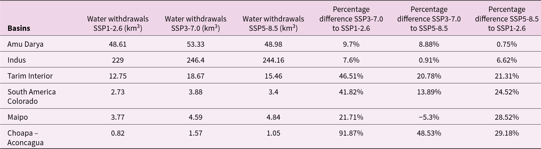
The left column of Figure 3 shows the annual water withdrawals from all sectors (Irrigation, Electricity, Municipal, Livestock, Mining, and Manufacturing) and the 10-year running mean of surface runoff under SSP1-2.6, SSP3-7.0, and SSP5-8.5 scenarios. In terms of annual WD, we can see in Figure 3 that in the case of Tarim Interior, South America Colorado, Maipo, and Aconcagua-Choapa SSP3-7.0 results in higher WD at the end of the 21st Century compared to SSP1-2.6 and SSP5-8.5 scenarios. The difference in average annual WD between SSP3-7.0 and the more sustainable scenario SSP1-2.6 in the 2050–2099 period is up to 91.8% more water withdrawals in the case of Choapa-Aconcagua, 46.5% in Tarim Interior, 41.8% in South America Colorado, and 21.7% in the Maipo basin (Table 2). On the other hand, the difference between the SSP5-8.5 and SSP1-2.6 in the same time period results in water withdrawals between 20% and 30% higher in the same basins. On the contrary, the differences between scenarios in the case of the Amu Darya and Indus basins are lower than 10% in both cases (SSP3-7.0 to SSP1-2.6 and SSP5-8.5 to SSP1-2.6).
Multi-model mean of annual water withdrawals, 10-year running mean of surface runoff and cumulative surface water deficit under SSP1-2.6, SSP3-7.0, and SSP5-8.5 in km3 for selected basins. The 10-year running mean is estimated from 2025 to 2100, given the need for at least 5 periods to estimate the average. Water withdrawals are estimated by GCAM, surface runoff by OGGM-Xanthos and cumulative surface deficits are estimated by the algorithm integrating GCAM with OGGM-Xanthos results.

Multi-model mean of water withdrawals under SSP1-2.6, SSP3-7.0, and SSP5-8.5 in km3 for selected basins during 2050–2099
Another aspect shown in Figure 3 is that the WD annual trend is highly specific for each basin and SSP scenario. We fit a Theil-Sen coefficient with Moving Block Bootstrapping (n = 300) in two periods (2020–2049 and 2050–2099) to estimate the annual variation and trend for each basin and SSP scenario. In the case of the Amu Darya and Indus Basin, their interannual WD variations are consistently less than 0.3% for Indus and less than 0.6% for Amu Darya in all SSP and both periods (2020–2049 and 2050–2099), with the majority of coefficients not statistically different from zero, suggesting a relatively stable WD (see Table S3 in the Supplementary Material). In the case of the Tarim Interior basin, our results show a negative trend in water withdrawals in the second half of the 21st century (2050–2099) of −1.5% (±0.14%) per year under SSP1-2.6 and −1.1% (±0.15%) per year under SSP5-8.5, meanwhile under SSP3-7.0 the trend is lower but still negative (−0.34% per year ±0.13%).
In the Andean region, we can see that in the cases of South America Colorado, Choapa-Aconcagua, and Maipo basins, under SSP1-2.6 and SSP5-8.5 scenarios, there is a positive trend in water withdrawals during the 2020–2049 period (0.70% [±0.20%], 0.31% [±0.07%], and 0.48% [±0.35%] per year under the SSP1-2.6, and 1.08% [±0.32%], 0.81% [±0.41%], and 1.27% [±0.45%] per year under the SSP5-8.5, respectively). In the second half of the 21st Century, this trend is reversed for the same basin under the same SSP scenarios. The estimated trend is −0.92% (±0.29%), −0.56% (±0.32%), and −0.82% (±0.3%) per year under SSP1-2.6 and −0.48% (±0.26%), and −0.52% (±0.42%) per year under SSP5-8.5 for South America Colorado and Maipo basins, respectively (Choapa – Aconcagua trend is not significantly different from zero [−0.34% ± 0.35%]).
In the center column of Figure 3, we can see the annual surface runoff for each basin under the three different SSP scenarios. In the case of the Indus basin, we can see an upward trend in the 10-year running mean of surface runoff in all three SSPs between the 2020 and 2100 period (see Table S4 in the Supplementary Material). In this basin, the trend is 0.19 (±0.17), 0.25 (±0.12), and 0.4 (±0.17) km3 per year for SSP1-2.6, SSP3-7.0, and SSP5-8.5.
In the case of the Amu Darya, our results show a negative trend in surface runoff of −0.18 (±0.12), −0.22 (±0.1), and −0.14 (±0.09) km3 per year between the 2020–2100 period under the SSP1-2.6, SSP3-7.0. In the case of Tarim Interior, a negative trend and statistically different from zero, under the SSP1-2.6 scenario of −0.18 (±0.12) km3 per year during the same period.
Finally, our analysis of the Chilean basins, including Choapa-Aconcagua and Maipo, indicates that the trends projected under the SSP1-2.6 scenario are not statistically different from zero. However, under SSP3-7.0 and SSP5-8.5, the trend in surface runoff is −0.016 (±0.007) and −0.026 (±0.012) km3 per year in Maipo and −0.0057 (±0.003) km3 per year in Choapa-Aconcagua under SSP5-8.5 scenario during the 2020–2100 period.
In the right column of Figure 3, we show the Cumulative Surface Water Deficit – CWD (here understood as when WD is greater than surface runoff plus storage release) for the 2020–2099 period under SSP1-2.6, SSP3-7.0, and SSP5-8.5 scenarios for the selected basins. In the Amu Darya, Indus, Tarim Interior, and Choapa-Aconcagua basins, the SSP3-7.0 scenario results in higher surface water deficits than the SSP1-2.6 and SSP5-8.5 scenarios. The difference in CWD at the end of the period (the cumulative deficit at 2099) between SSP3-7.0 and SSP1-2.6 is 856% in Amu Darya, 14.4% for Indus, 238.8% for Tarim Interior, and 1041.1% for Choapa-Aconcagua basin. This difference is lower, but still relevant, between SSP5-8.5 and SSP1-2.6 scenarios, with 469.3%, 10.2%, 39.8%, and 341.9% of higher CWD for each respective basin.
In the Maipo basin, the SSP5-8.5 scenario results in higher surface water deficits than SSP1-2.6 and SSP3-7.0, with 231.1% more CWD than the former and 50.1% more than the latter scenario.
On the other hand, in the case of the South American Colorado basin, our results show that surface water deficits are zero as the available surface runoff is enough to meet the water withdrawal demand estimated by GCAM.
In the same column of Figure 3, we can also observe consistently increasing surface water deficits in the Indus, Maipo, and Choapa-Aconcagua basins, particularly under the SSP3-7.0 and SSP5-8.5 scenarios (and SSP1-2.6 only in the case of Indus basin). On the other hand, in the case of the Tarim Interior basin, we can see a stabilization of the surface water deficit near 2040 in the SSP1-2.6 and SSP5-8.5 scenarios and near 2050 in the SSP3-7.0 scenario. This stabilization can be explained by the projected reduction of surface water withdrawal in the second half of the 21st century below their historical values, while surface runoff remains close to historical values during the same period.
For most of the selected basins, irrigation water requirements represent the most relevant sector of water withdrawals. In Asian basins (Amu Darya, Indus, and Tarim Interior), it averages at least 80% of the annual water withdrawals for the 2020–2099 period for all three SSPs scenarios. The same applies to the South America Colorado basin, where the irrigation sector withdraws at least 67% on average in the selected SSPs (see Tables S6–S8 in the Supplementary Material).
In the case of the Choapa-Aconcagua basin, irrigated croplands represent at least 30% of annual water withdrawals under SSP1-2.6 and SSP5-8.5 but 57% of annual withdrawals under the SSP3-7.0 scenario. On the other hand, the case of the Maipo basin presents a different profile, with, on average, 35% of the total water withdrawals required for irrigated croplands under all SSPs and the Manufacturing sector represents 30% of the total.
Figure 4 shows the quantity of land used for irrigated cropland under the SSPs scenarios for the selected basins. The SSP3-7.0 scenario results in higher irrigated land use in all basins compared to the SSP1-2.6 and SSP5-8.5 scenarios. Furthermore, there are negative trends in irrigated land use under the latter two scenarios across all basins analyzed, whereas some basins exhibit an increase in irrigated land use under the SSP3-7.0 scenario.
Multi-model mean annual irrigated cropland area under SSP1-2.6, SSP3-7.0, and SSP5-8.5 in thousand km2 for selected basins.

In the cases of the Amu Darya and South America Colorado basins, the SSP3-7.0 scenario exhibits a positive trend in irrigated land use in the entire 2020-2099 period. On the other hand, in the Indus, Tarim Interior, Maipo, and Choapa–Aconcagua, there is an initial positive trend in irrigated land use under SSP3-7.0 and a posterior decline in the total land used for irrigated crops in the second half of the 21st Century.
3.2. Glacier runoff changes under SSP scenarios
As shown in Figure 5, in most of the basins selected here, monthly glacier runoff maximums coincide with months with high water withdrawal requirements, commonly associated with irrigation requirements in the driest season. In the case of the Amu Darya and Tarim Interior basins, both water withdrawals and glacier runoff reach their annual maximum between June and July. In the case of the Indus basin, although glacier runoff peaks during June–July, the Kharif-Rabi irrigation pattern produces peaks in water withdrawals during March–April and September–October, respectively. Finally, in the case of South America Colorado, Maipo, and Choapa-Aconcagua basins, both water withdrawals and glacier runoff peak between December and January, coinciding with the Southern Hemisphere summer season.
Multi-model mean monthly water withdrawals and glacier runoff between 2020 and 2099 under SSP1-2.6, SSP3-7.0, and SSP5-8.5 in km3 for selected basins. Note that y-axis ranges differ across panels to preserve the visibility of seasonal variability in Glacier runoff estimations.

Figure 5 shows that glacier runoff represents a relatively small fraction of the monthly total surface runoff across the studied basins. Hence, precipitation and snowmelt are the dominant contributors to surface runoff in these regions. Nonetheless, in the Amu Darya, Tarim Interior, South America Colorado, Choapa-Aconcagua, and Maipo basins, glacier runoff peaks coincide more closely with periods of high irrigation demand, although their overall contribution remains smaller than that of precipitation and snow-derived runoff.
Glacier runoff is expected to peak during the 21st Century under climate change scenarios, particularly in the case of the basins selected in this study. Using the 10-year multi-model mean annual glacier runoff, as shown in Figure 6, we can identify that under the SSP3-7.0 and SSP5-8.5 scenarios, there is a peak-water glacier runoff between 2040 and 2060 in the Amu Darya, Indus, Tarim Interior, South America Colorado, Maipo, and Choapa-Aconcagua basins. After the peak, a negative trend in annual glacier runoff is consistently observed in these basins, causing glacier runoff to fall below the initial values.
10-year running multi-model mean of annual glacier runoff under SSP1-2.6, SSP3-7.0, and SSP5-8.5 in km3 for selected basins between 2025 and 2099. The 10-year running mean is estimated from 2025 to 2099, given the need for at least five periods to estimate the average.

Under the SSP1-2.6 scenario in the Indus and Tarim Interior basins, the peak water glacier runoff occurrence is less apparent as there is no statistically significant and positive trend between 2020 and 2049 that suggests an acceleration of glacier melt. However, the negative trend of glacier runoff between 2050 and 2099 under this scenario is −0.07 (±0.01) km3 per year in the Indus basin and −0.21 (±0.03) km3 per year in the case of the Tarim Interior (see Table S5 in the Supplementary Material for details). In the case of Amu Darya, there are negative and statistically significant trends in both periods under SSP1-2.6, with −0.03 (±0.01) km3 per year between 2020 and 2049 and −0.06 (±0.009) km3 per year between 2050 and 2099. Although the statistical approach used here does not identify a distinct ‘peak water’ period, the temporal evolution of glacier runoff still shows a clear maximum contribution followed by a subsequent decline, indicating that a maximum glacier runoff does occur but is less evident compared to SSP3-7.0 and SSP5-8.5 scenarios.
Under SSP5-8.5 in the Amu Darya and Tarim Interior basins, we see evidence of Peak-Water Glacier Runoff occurrence with maximums of the contribution of the glacier to runoff near the middle of the 21st century and positive trends in glacier runoff between 2020 and 2049 (0.019 (±0.01) and 0.18 (±0.9) km3 per year, respectively) and negative trends between 2050 and 2099 (−0.1 (±0.01) and −0.3 (±0.03) km3 per year, for Amu Darya and Tarim Interior, respectively). Under SSP3-7.0, our results show the same pattern for the Tarim Interior basin with a positive trend between 2020 and 2049 (0.14 [±0.06] km3 per year) and a negative trend in the second half of the 21st century (−0.23 [±0.02] km3 per year).
In the case of Andean basins, as shown in Figure 6, we can see that scenarios SSP3-7.0 and SSP5-8.5 also produce faster declines of annual glacier runoff causing it to fall below the SSP1-2.6 estimates and approach zero at the end of the 21st Century. Although given the earlier Peak-Water Glacier Runoff occurrence in the case of Choapa-Aconcagua, Maipo, and South America Colorado basin, a positive and statistically significant trend is found in the 2020–2039 period instead of the 2020–2049 period as is the case of Asian basins. In the rest of the 21st century (2040–2099), a statistically significant and negative trend is observed in the same basins.
4. Discussion and conclusions
In this article, we present surface runoff estimations under three SSP scenarios (SSP1-2.6, SSP3-7.0, and SSP5-8.5) using a modified version of the ABCDM model within the Xanthos framework that now includes glacier runoff as input from the OGGM glacier model. We use GCAM to estimate water withdrawals for six sectors (Irrigation, Municipal, Manufacturing, Mining, Electricity, and Livestock) and use Demeter and Tethys tools to temporal and spatial downscale these results into a monthly gridded (0.5°) dataset. Finally, we estimate the water balance and deficit of the selected basins considering their reservoir capacity.
Regarding water withdrawals, the SSP3-7.0 scenario results in higher estimates than the SSP1-2.6 and SSP5-8.5 scenarios for most of the selected basins. These results are explained mainly due to the SSP assumptions in the GCAM implementation of these scenarios, as SSP3-7.0 is associated with higher population growth (up to 12.7 billion people), lower Gross Domestic Product per capita, low agricultural productivity growth, high meat demand, no land conservation or reforestation policy and larger irrigated cropland area (JGCRI, 2023). An exception is the Maipo basin, where SSP5-8.5 leads to higher water withdrawals than SSP3-7.0 due to the basin’s specific withdrawal profile, where manufacturing is as significant as irrigation.
Regarding surface runoff, under all SSP scenarios analyzed here in the Indus basin, our results show an increasing trend during the 21st century related to the increase in precipitation projected in this region under climate change scenarios (Chen et al., Reference Chen, Zhou, Zhang, Chen, Zhang and Jiang2020a; Cook et al., Reference Cook, Mankin, Marvel, Williams, Smerdon and Anchukaitis2020; Zhai et al., Reference Zhai, Mondal, Fischer, Wang, Su, Huang, Tao, Wang, Ullah and Uddin2020). In the case of the Amu Darya, Maipo, and Choapa-Aconcagua basins, we can see a negative trend in surface runoff, particularly in the second half of the 21st century under most of the SSP scenarios. In the case of the Chilean basins (Maipo and Choapa-Aconcagua), this result is consistent with the projection of lower precipitation under SSP scenarios (Salazar et al., Reference Salazar, Thatcher, Goubanova, Bernal, Gutiérrez and Squeo2024). Finally, in the Amu Darya basin, climate projections have high uncertainty, and although some scenarios (particularly, SSP3-7.0 and SSP5-8.5) produce slightly more precipitation at the end of the 21st century, the increase in temperature under the same scenarios increases evapotranspiration and, hence, can explain the decrease in runoff observed in our results (Chen et al., Reference Chen, Zhou, Zhang, Chen, Zhang and Jiang2020b; Cook et al., Reference Cook, Mankin, Marvel, Williams, Smerdon and Anchukaitis2020).
Regarding surface water deficit, SSP3-7.0 results in highest cumulative surface water deficits for most of the selected basins (Amu Darya, Indus, Tarim Interior, and Choapa-Aconcagua), whereas SSP5-8.5 results in higher deficits in the case of Maipo basin. The latter results can be explained by the combination of the higher proportion of manufacturing water withdrawals (expected to increase under SSP5 assumptions), a lower proportion of irrigation water requirements, and a lower surface runoff under the SSP5-8.5 scenario in this basin. These results are consistent with previous literature in which SSP3 has also been identified as a scenario with higher water withdrawals and water scarcity compared with other SSP scenarios (Graham et al., Reference Graham, Hejazi, Chen, Davies, Edmonds, Kim, Turner, Li, Vernon, Calvin, Miralles-Wilhelm, Clarke, Kyle, Link, Patel, Snyder and Wise2020; Hanasaki et al., Reference Hanasaki, Fujimori, Yamamoto, Yoshikawa, Masaki, Hijioka, Kainuma, Kanamori, Masui, Takahashi and Kanae2013; Satoh et al., Reference Satoh, Kahil, Byers, Burek, Fischer, Tramberend, Greve, Flörke, Eisner, Hanasaki, Magnuszewski, Nava, Cosgrove, Langan and Wada2017).
Graham et al. (Reference Graham, Hejazi, Chen, Davies, Edmonds, Kim, Turner, Li, Vernon, Calvin, Miralles-Wilhelm, Clarke, Kyle, Link, Patel, Snyder and Wise2020) attributed whether water withdrawals (Human component) or water availability (Climate component) increased or decreased water scarcity under the SSP scenarios. Our results are consistent with Graham et al. (Reference Graham, Hejazi, Chen, Davies, Edmonds, Kim, Turner, Li, Vernon, Calvin, Miralles-Wilhelm, Clarke, Kyle, Link, Patel, Snyder and Wise2020) estimates in the case of the Maipo, Choapa-Aconcagua, and South America Colorado basins in which water withdrawals increase, particularly under the SSP3-7.0 scenario, and surface runoff decreases, particularly under SSP3-7.0 and SSP5-8.5 scenarios, increasing surface water deficit.
In the case of the Indus basin, our results also show that surface runoff increases during the 21st century, similar to the trend identified by Graham et al. (Reference Graham, Hejazi, Chen, Davies, Edmonds, Kim, Turner, Li, Vernon, Calvin, Miralles-Wilhelm, Clarke, Kyle, Link, Patel, Snyder and Wise2020), in which the Climate component decreases water scarcity. However, our results show small variations in water withdrawals under all SSPs with a low, although still positive, trend in water withdrawals, in contrast to Graham et al. (Reference Graham, Hejazi, Chen, Davies, Edmonds, Kim, Turner, Li, Vernon, Calvin, Miralles-Wilhelm, Clarke, Kyle, Link, Patel, Snyder and Wise2020) results that attribute a positive signal to the Human component (increasing water scarcity). This relative stability of water withdrawals can be explained by the fact that water withdrawals estimated by GCAM are consistently above the surface availability estimated with OGGM-Xanthos models, hence contributing to a higher surface water deficit, but also limiting GCAM to increase water withdrawals due to higher water extraction-related costs. These results are different from the default GCAM SSP results or Graham et al. (Reference Graham, Hejazi, Chen, Davies, Edmonds, Kim, Turner, Li, Vernon, Calvin, Miralles-Wilhelm, Clarke, Kyle, Link, Patel, Snyder and Wise2020) estimates, given that our surface water availability estimates are smaller. Nonetheless, even if water availability increases and water withdrawal remains relatively constant, cumulative surface water deficit consistently increases for this basin in all SSPs included in this study. This study estimated glacier runoff using the OGGM glacier model under the same SSP scenarios. Our findings reveal that the monthly maximum glacier runoff aligns with peak irrigation WD in most of the analyzed basins. Moreover, our results also show that glacier runoff is expected to peak, known as peak-water glacier runoff, during the 21st century under SSP3-7.0 and SSP5-8.5. This is consistent with previous literature that has projected a faster melting of glaciers worldwide, causing a peak glacier runoff and a subsequent decline of glacier contribution to runoff (Bliss et al., Reference Bliss, Hock and Radić2014; Caro et al., Reference Caro, Condom, Rabatel, Champollion, García and Saavedra2024; Huss & Hock, Reference Huss and Hock2018; Wimberly et al., Reference Wimberly, Ultee, Schuster, Huss, Rounce, Maussion, Coats, Mackay and Holmgren2025).
Although our results show a strong temporal alignment between glacier runoff peaks and peak irrigation withdrawals in most of the studied basins (with the exception of the Indus, where the Rabi season peak in irrigation aligns more closely with precipitation), glacier runoff remains a secondary source of surface runoff compared to precipitation and snowmelt.
Overall, water withdrawals represent the primary source of variation between the SSPs analyzed in this study. This can be exemplified when comparing the SSP3-7.0 and SSP5-8.5 scenarios. While surface runoff exhibits similar trends in both scenarios, the variation in surface runoff is smaller compared to the differences in water withdrawals. As a result, the observed disparities in surface water deficit are likely more associated with changes in water withdrawals than with fluctuations in surface runoff. This is consistent with the previous literature, which has identified the anthropic component as the major source of water scarcity under climate change scenarios (Graham et al., Reference Graham, Hejazi, Chen, Davies, Edmonds, Kim, Turner, Li, Vernon, Calvin, Miralles-Wilhelm, Clarke, Kyle, Link, Patel, Snyder and Wise2020; Hanasaki et al., Reference Hanasaki, Fujimori, Yamamoto, Yoshikawa, Masaki, Hijioka, Kainuma, Kanamori, Masui, Takahashi and Kanae2013).
One limitation of this study arises from the irrigation water withdrawal estimation from GCAM. As the Data and Methods section explains, GCAM uses exogenous WD coefficients for each crop type and assumes that green water (i.e., water from precipitation stored in the soil used by crops in their growth process) maintains historical levels in each basin. Hence, if climate change significantly changes a basin's precipitation regime and soil moisture drivers, green water changes accordingly, and irrigation WD could be under or overestimated.
A second limitation of our study concerns the potential double-counting of the snowfall component of glacier runoff over glacierized areas. The potential overestimation of glacier runoff implies that our estimates of glacier contributions to total runoff and surface water deficits analysis should be interpreted with caution. Although the calibration of the M parameter reduces the magnitude of this bias, a residual effect may persist. Further studies should focus on improving the coupling between OGGM and the Xanthos hydrological model to achieve a more consistent treatment of snowfall inputs and melt processes across the modeling framework.
Uncertainties in this study also stem from the fact that the THETYS-based downscaling assumes that the spatial distribution of withdrawals within each basin remains constant over time, which may introduce bias in rapidly changing regions. Similarly, representing all reservoirs as a single aggregated storage unit per basin simplifies water management processes but is appropriate for basin-scale analyses, where both runoff and demand are spatially integrated. Future work should explore the use of spatially explicit reservoir data and dynamic downscaling frameworks to better capture intra-basin variability and improve the robustness of surface water deficit projections.
In basins with increasing precipitation but moderate soil moisture increases, especially in the Indus basin, irrigation water withdrawals may be lower than projected. Conversely, in regions like the Chilean Andean basins, where precipitation and soil moisture both decline, irrigation demand might be higher than GCAM estimates suggest. This discrepancy introduces uncertainty into our water withdrawal projections and highlights the need for more dynamic models that account for climate-driven changes in both blue and green water availability. Future research should incorporate more flexible irrigation demand estimations that consider changes in precipitation, soil moisture, and technological conditions to improve our understanding of the impacts derives from climate change scenarios.
This study utilized global datasets to ensure consistency in the assessment of two distinct world regions: Asia and South America. While the 0.5° spatial resolution allows for the analysis of Chilean basins – many of which are not included in the original GCAM macro-regions – this resolution remains coarse relative to the actual size of basins located west of the Andes Cordillera, such as those in Chile and Peru. Future work could address this limitation by employing finer spatial resolutions in these basins; however, this would reduce comparability between the Asian and South American assessments, as globally consistent data on water withdrawals, water storage, cropland, and climate are not available at resolutions finer than 0.5°.
The results presented here, based on the five GCMs selected by ISIMIP3b as climate forcings, reveal substantial uncertainty in the estimates of glacier and surface runoff. This uncertainty propagates to the cumulative surface water deficit estimates. However, while in the Indus and Amu Darya basins water withdrawal estimates show greater variability, narrower uncertainty ranges are observed for this variable in the remaining basins. This pattern may be attributed to the higher sensitivity of the Indus and Amu Darya basins to changes in surface water availability, while the other basins demonstrate a more stable response, consistent with findings from previous studies (Cui et al., Reference Cui, Calvin, Clarke, Hejazi, Kim, Kyle, Patel, Turner and Wise2018).
Based on these findings, two main policy implications arise. First, effective and large-scale mitigation measures must be implemented to reduce the probability of severe climate change scenarios (SSP3-7.0 and SSP5-8.5), especially to avoid the occurrence of the peak-water glacier runoff and the loss of the buffer capacity of glaciers during the driest month of the year observed under these scenarios. Second, given that water withdrawal is the main driver of water scarcity (especially irrigation water withdrawals), there is an urgent need to implement effective adaptation measures to reduce water withdrawals through more efficient irrigation practices and improved water-use efficiency across sectors.
Supplementary material
The supplementary material for this article can be found at https://doi.org/10.1017/sus.2025.10046.
Acknowledgements
The authors acknowledge the support of the Center for Climate and Resilience Research – CR2 (FONDAP 1523A0002, National Agency of Research and Development of Chile).
Author contributions
Rubén Calvo-Gallardo and Fabrice Lambert participated in the Conceptualization, Methodology, and Writing – original draft and the Writing – review and editing. Rubén Calvo-Gallardo also performed the Data curation, Software development, Formal Analysis, and Visualization. Anahí Urquiza and Nicolás Álamos participated in this work’s Conceptualization, Methodology, Writing – review, and editing.
Financial support
Rubén Calvo-Gallardo acknowledges the National Agency of Research and Development of Chile’s national Ph.D. funding. Scholarship Program no. 21,200,800 (ANID-PFCHA/Doctorado Nacional/2020-21200800). The authors acknowledge the funding provided by the ‘Programa de Estímulo a la Excelencia Institucional (PEEI) de la Universidad de Chile, Facultad de Ciencias Agronómicas’. The authors acknowledge the funding by the FONDECYT Project no. 1,231,682 of the National Agency of Research and Development of Chile. The authors acknowledge the funding provided by the ‘Proyecto FIDA 2021 Fortalecimiento académico de la Facultad de Ciencias Agronómicas en el ámbito de la innovación y de la gestión rural, Universidad de Chile’.
Conflict of interest
The authors declare no conflicts of interest relevant to this study.
Data availability
The databases required to reproduce the results from this article are available at https://zenodo.org/records/17953249.


 Open access