


1. INTRODUCTION
Glaciers are dynamic systems that are in constant motion. Their movement, changes in their stress regime, cracks and crevasse expansion, iceberg calving and ice-basal friction all release energy, which can release detectable seismic signals across a broad frequency range (from seismic to seismo-acoustic). Therefore, glacial seismicity has been studied over many years with growing interest.
There are numerous kinds of seismic events, which have been identified in glaciated areas. For this paper the most important are: icequakes, iceberg calving, calving earthquakes, seiches, glacier tremors and ice-vibrations. Pioneering studies on icequakes were conducted in the 1960s and 1970s (Lewandowska and Teisseyre, Reference Lewandowska and Teisseyre1964; Neave and Savage, Reference Neave and Savage1970; Cichowicz, Reference Cichowicz1983). The authors characterised basic icequake parameters and related them to ice movement and internal ice stress changes. The second type of event, iceberg calving, was studied as another type of glacier-generated signal (Qamar, Reference Qamar1988; Amundson and others, Reference Amundson2008; O'Neel and others, Reference O'Neel, Larsen, Rupert and Hansen2010; Köhler and others, Reference Köhler, Nuth, Schweitzer, Weidle and Gibbons2015; Bartholomaus and others, Reference Bartholomaus2015b). Temporal seismic and acoustic calving monitoring using receivers located in close proximity to calving fronts was later introduced by O'Neel and others (Reference O'Neel, Marshall, McNamara and Pfeffer2007), Richardson and others (Reference Richardson, Waite, Fitzgerald and Pennington2010) and Glowacki and others (Reference Glowacki2015). Calving of a massive iceberg in a fjord generates very low-frequency seiche waves, which can be monitored from greater distances using broadband seismometers (Amundson and others, Reference Amundson2012; Walter and others, Reference Walter, Olivieri and Clinton2013). All these studies reveal the diversity of calving-related waveform characteristics depending on the type of calving event (Tsai and others, Reference Tsai, Rice and Fahnestock2008; Köhler and others, Reference Köhler, Chapuis, Nuth, Kohler and Weidle2012, Reference Köhler, Nuth, Schweitzer, Weidle and Gibbons2015). Calving of extremely large iceberg can cause glacial earthquakes of considerable magnitude (M L ≥ 5) in seismological terms (Ekström and others, Reference Ekström, Nettles and Tsai2006), however their focal mechanisms are continuously debated. Different kind of signals, narrow-banded seismic tremors lasting from seconds to even several hours (Métaxian and others, Reference Métaxian, Araujo, Mora and Lesage2003; O'Neel and Pfeffer, Reference O'Neel and Pfeffer2007; Röösli and others, Reference Röösli2014) were proposed to be caused by a resonance in fluid-filled cracks (Lipovsky and Dunham, Reference Lipovsky and Dunham2015) and to be related to subglacial water discharge (Bartholomaus and others, Reference Bartholomaus2015a). Another type of monochromatic event is a low-frequency ice-vibration, which is likely caused by large-scale dynamic processes within the glacier, for example the displacement of a considerable part of the glacier due to gravity or uplift forces (Górski and Teisseyre, Reference Górski and Teisseyre1991; Górski, Reference Górski2004). The spectral characteristics of ice-vibrations vary between different glaciers, mainly due to varying glacier size and have been detected in tidewater, as well as in alpine glaciers. Górski (Reference Górski2004) determined the approximate location of these events on the Hansbreen glacier at a distance from its calving front using an array of seismometers. For a more detailed insight into seismological research in the field of glaciology the interested reader is referred to a recent comprehensive review of cryoseismology by Podolskiy and Walter (Reference Podolskiy and Walter2016).
The number of seismic events generated by glaciers, change dramatically during the year with a peak during late summer (Ekström and others, Reference Ekström, Nettles and Tsai2006; O'Neel and others, Reference O'Neel, Larsen, Rupert and Hansen2010, Köhler and others, Reference Köhler, Nuth, Schweitzer, Weidle and Gibbons2015). Seasonal changes can be studied using dedicated local seismic networks targeting the detection and location of glacier-induced seismicity (e.g., Köhler and others, Reference Köhler, Chapuis, Nuth, Kohler and Weidle2012; Bartholomaus and others, Reference Bartholomaus2015b; Koubova, Reference Koubova2015); but, due to their temporary deployment, these networks cannot capture a full record of interannual changes. However, there is a wealth of the seismological data available from permanent stations located in the polar regions that have been recording continuous data streams over many years. Some of these stations are located near glaciers, making the detection of glacier-induced seismic events feasible. Recent studies by Köhler and others (Reference Köhler, Nuth, Schweitzer, Weidle and Gibbons2015, Reference Köhler2016) utilise seismological station records to assess interannual calving intensity at two locations from Spitsbergen. The key aspect related to the use of seismological observations for glaciers’ monitoring is the development of the robust detection and classification scheme that enables to distinguish a glacier-related event from other events like human origin disturbances or tectonic earthquakes.
In this paper, we describe an algorithm for single-station automatic seismic event detection and classification for continuous seismological records. The classification algorithm utilises fuzzy logic, while classification rules are based on theoretical knowledge and verified using a set of confirmed calving icequakes reported by Köhler and others (Reference Köhler, Nuth, Schweitzer, Weidle and Gibbons2015). We apply the developed algorithm to continuous long-term records from two permanent seismic stations located in Spitsbergen in the vicinity of glaciers. Obtained distributions of glacier-induced seismicity reveal several correlations with glaciological and meteorological data.
2. DATA
The analysed data were recorded at Spitsbergen (Fig. 1a), the largest island of the Svalbard Archipelago (Norway), which is a seismically active region located in the Arctic in the vicinity of the Knipovich and Gakkel Ridges, where oceanic spreading centres constantly generate tectonic earthquakes (Engen and others, Reference Engen, Eldholm and Bungum2003). The most active seismic zones in Svalbard are Heer Land, Nordaustlandet (Mitchell and others, Reference Mitchell, Bungum, Chan and Mitchell1990) and Storfjorden, the latter being recently affected by a sequence of earthquakes, with the largest reaching a local magnitude of M L = 6.0 (Pirli and others, Reference Pirli, Schweitzer and Paulsen2013). This relatively high seismic activity makes it challenging to distinguish between earthquakes and glacier-related events. Thus, this is a good testing area for the method's performance. Spitsbergen is also the study area for many previous papers focussed on glacier-related seismicity. Recently, Köhler and others (Reference Köhler, Nuth, Schweitzer, Weidle and Gibbons2015) carried out a study of glacier seismicity in the Spitsbergen, providing a unique opportunity to verify our classification algorithm and compare results obtained using two independent methods. The proximity of seismic stations to the large glacial systems makes Spitsbergen's conditions suitable for our research.
Study area: (a) general map of Svalbard with the KBS and HSPB seismological stations marked with red dots. (b) Enlarged KBS station area. (c) Enlarged HSPB station area. Modified from an online Map of Svalbard: http://toposvalbard.npolar.no/.
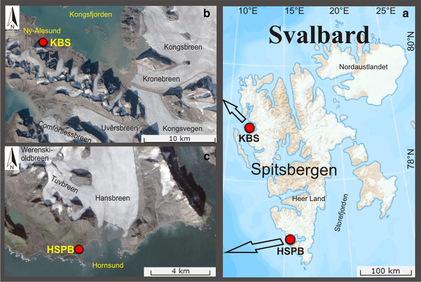
We used continuous seismic records from two seismological broadband stations, HSPB and KBS, which are located in Spitsbergen (Fig. 1). The HSPB station is located in the Hornsund fjord near the Polish Polar Station in southern Spitsbergen. This station belongs to the Polish Seismological Network (PL), which is operated by the Institute of Geophysics, Polish Academy of Sciences (IG PAS). In 2007, as part of the International Polar Year activities, the station was upgraded with the help of the NORSAR organisation, and a three-component (3C) broadband seismometer (STS-2) with sampling rate of 100 Hz was installed. This enabled the analysis of distant (teleseismic) earthquakes (e.g., Wilde-Piórko and others, Reference Wilde-Piórko, Grad, Wiejacz and Schweitzer2009).
The HSPB station is located near the Hansbreen glacier, the largest glacier in the area (Fig. 1c). The distance to its terminus is ~3 km. Hansbreen is a 16 km long polythermal tidewater glacier covering an area of 56 km2. Its frontal cliff is ~1.5 km wide and 30 m a.s.l. (Błaszczyk and others, Reference Błaszczyk, Jania and Hagen2009; Grabiec and others, Reference Grabiec, Jania, Puczko, Kolondra and Budzik2012). Another glaciers to the north from the station are Tuvbreen (tributary of Hansbreen) and Werenskioldbreen.
The KBS station is located in Kongsfjorden, Ny-Ålesund, in western Spitsbergen (Fig. 1b). The KBS station belongs to the Norwegian National Seismological Network. It is operated by the University of Bergen and equipped with the same type of broadband seismometer (STS-2) with sampling rate of 40 Hz.
The largest glaciers in the proximity of the station are Kronebreen, Kongsvegen, Kongsbreen, Uvêrsbreen, Blomstrandbreen and Comfortlessbreen (Fig. 1b). The distance to the combined terminus of Kronebreen and Kongsvegen is ~15 km. The Kronebreen's surface is 445 km2 (Trusel and others, Reference Trusel, Powell, Cumpston and Brigham-Grette2010) and it contributes significantly to the overall area of the local glacial system.
Both datasets are freely available online at various seismological open data repositories, for example through the IRIS data management centre (http://ds.iris.edu/ds/nodes/dmc/). In case of the HSPB station, we used the data recorded between 2010 and 2014, available in the online Orfeus database (http://www.orfeus-eu.org/). Data recorded between 2008 and 2009 were taken from an in-house seismological database at the IG PAS. Due to the lack of data in the last quarter of 2009 (due to the station maintenance), we used the last quarter of 2007 instead to show year-to-year comparisons and overall statistics in order to maintain unbiased data.
In case of the KBS station, we processed the data between 2010 and 2014. The analysed period differs from the HSPB station due to a lack of continuous KBS raw data in the online IRIS database.
The meteorological data for the Hornsund region comes from the GLACIO-TOPOCLIM database (http://www.glacio-topoclim.org/ – currently unavailable online), while the dataset for Ny-Ålesund was downloaded from the eKlima (http://www.eklima.met.no/) service.
3. METHODOLOGY
Seismic signals of various origins, referred to hereafter as ‘events’, were expected to occur in the analysed datasets. First, there are signals of glacial origin that we focus on in this study and records of local, regional and teleseismic earthquakes, which are the main objectives of seismological measurements. There are also signals of anthropogenic origin or those caused by natural phenomena other than glacier activity, such as ocean waves, hail, animals, etc., which we treat as disturbances. Our intent is to automate the processing of large volumes of continuous data for the detection and classification of glacier-induced seismic events. The sequence of processing procedures and their parameters were chosen to produce an autonomous processing sequence, which is easy to implement for any dataset. Each dataset was processed with strictly the same procedure and parameters to provide results that would not be biased by data processing. A two-step data analysis procedure consisted of the following: (1) basic event detection; and (2) fuzzy logic event classification. The following subchapters contain a detailed description of our processing scheme.
3.1. Basic event detection workflow
At this stage, the following five processing steps were applied to the data:
(1) Bandpass filtering (Butterworth filter with cut-off frequencies of 1 and 15 Hz);
(2) Detection based on the ratio of short-term average to long-term average (STA/LTA) of the signal;
(3) Multiple detection removal;
(4) Elimination of the weakest events;
(5) Estimation of the duration times of detected events and the elimination of events with duration times longer than 25 s.
A similar procedure is often used in earthquake seismology in a variety of approaches, and it is commonly implemented in more advanced acquisition systems to routinely pre-process the data stream from a seismic network. It was also used in the context of calving by Walter and others (Reference Walter, Olivieri and Clinton2013), but their study was focussed on detecting seiches - normal modes of fjord waters induced by calving. Although the general processing scheme was the same as ours, seiches have very low frequency content and require another parameterisation.
The first step of our workflow – bandpass filtering – was chosen to preserve the frequency bands of expected glacier-generated signals (Górski, Reference Górski2004; O'Neel and Pfeffer, Reference O'Neel and Pfeffer2007; O'Neel and others, Reference O'Neel, Marshall, McNamara and Pfeffer2007; Walter and others, Reference Walter2010; Köhler and others, Reference Köhler, Nuth, Schweitzer, Weidle and Gibbons2015) and to remove low-frequency microseisms generated by ocean waves, low frequency signals from teleseismic earthquakes (Stein and Wysession, Reference Stein and Wysession2003) and high-frequency noise.
For the 1–15 Hz filtered data, we ran a standard STA/LTA (Allen, Reference Allen1978) detection algorithm on each component of the signal independently. Each time the ratio of running averages exceeded the chosen threshold, a detection was triggered. Then, multiple detections were removed by introducing a compulsory 5 s offset between subsequent detections. All of the remaining detections were saved as 50 s intervals of 3C records.
Then, the weakest events with low signal-to-noise ratios (SNR) within the saved interval were eliminated, because they were prone to be not reliably described by energy flow parameters. We calculated a mean power (energy per time) of the whole 50 s record and the mean temporal power over short time intervals. Events with no interval of signal power exceeding the whole record mean power value by at least 30% were discarded as unreliable and noisy.
For each remaining event, we calculated its duration time by applying a modified normalised energy density (NED) function (Sarma, Reference Sarma1971). The original NED function is given by
 $$NED(t) = \sum\limits_{n = 1}^t {\left( {U(n)} \right)^2}, $$
where n is a signal sample index, U(n) is ground velocity at sample n, t is a time index within a selected time window. NED is a cumulative sum of energy calculated from some arbitrary starting time. As we are not interested in nominal values of the energy, the obtained function is then normalised to one and plotted versus time (or sample index). The steeper its slope ascents the more energy is being recorded. The slope of the function in the earthquake occurrence time interval was originally used to calculate the energy flux and the duration of strong earthquakes. However, in our case, the signal was often not much stronger than the noise, which results in a significant contribution from noise energy to the NED function. Thus, to remove the background noise influence, which was negligible for strong earthquakes considered by Sarma (Reference Sarma1971), we modified NED by subtracting a linear noise function (with slope N F). The value N F was calculated for each event using 4 s long signal interval (400 samples for 100 Hz sampled signal) 16 s prior to triggered detection by:
 $$N_F = \displaystyle{{\sum\limits_{n = 1}^{400} {\left \vert {U(n)} \right \vert}} \over {400}}$$
Then the modified mNED function was calculated for each time sample t in each of the extracted 50 s records using the following equation:
 $$mNED(t) = \sum\limits_{n = 1}^t {\left \vert {U(n)} \right \vert - N_F \cdot t}. $$
The character of mNED function and the effect of N F subtraction is well visible in Figure 2, where mNED function without N F subtraction rises significantly in the pre-event time interval. After N F subtraction, most of the mNED function value change is related to the energy of the event, not the noise.
(a) Example of a 1–15 Hz filtered seismogram with a recorded event; (b) mNED with N F = 0 (no noise subtraction) for the seismogram above – blue solid line, linear noise function – black dashed line; (c) mNED function (after noise correction) – blue solid line. The mNED limits of 0.15 and 0.85 that were used for the duration time estimation - orange dashed lines.
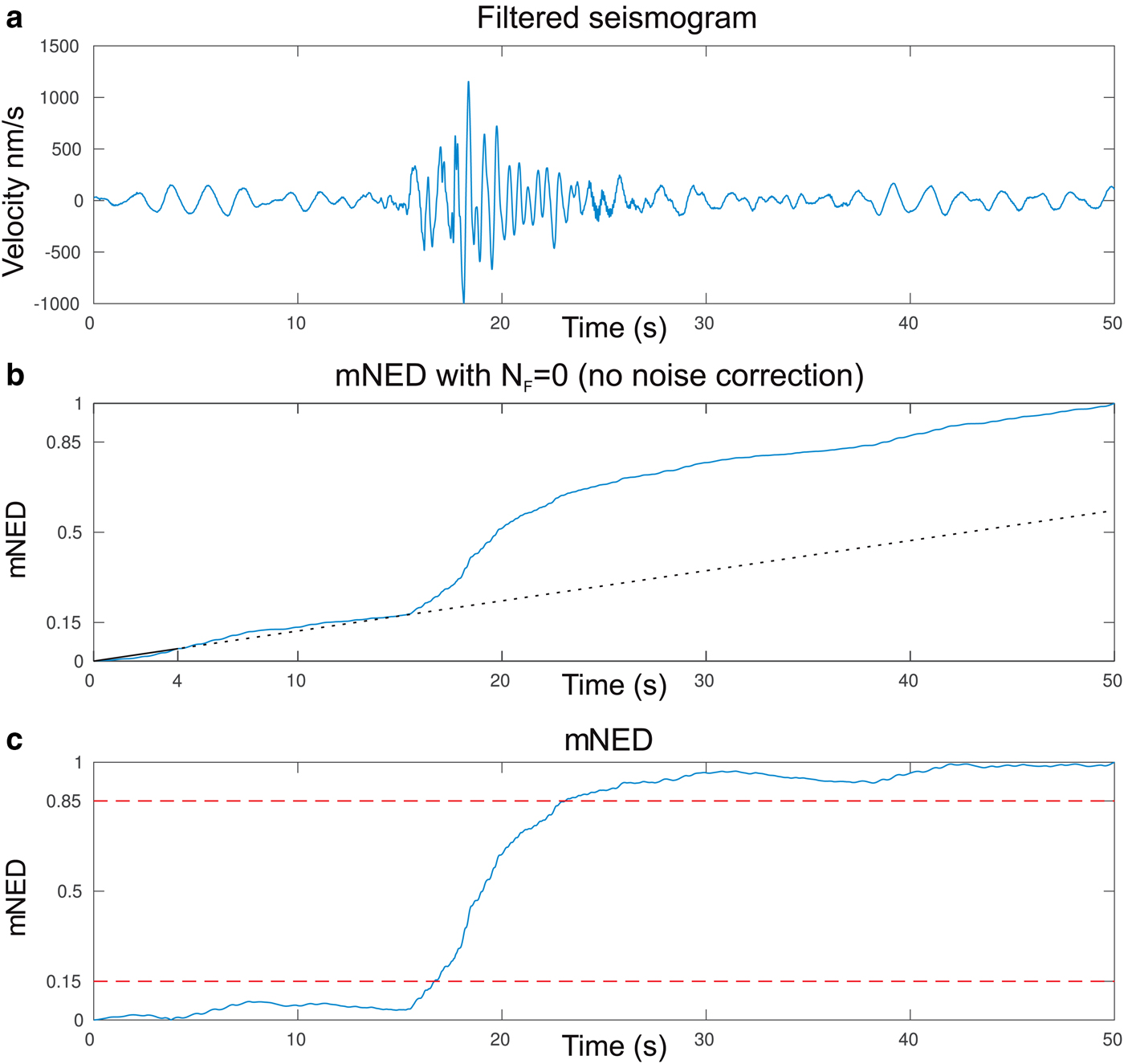
We defined the time needed for mNED to rise from a value of 0.15–0.85 as the duration time of the event. Theoretically, for small amounts of noise, this limit could be relaxed (i.e., the lower limit could be closer to 0 and the higher limit could be closer to 1), but the chosen limits constrain the function to be more resistant to occasional rapid noise fluctuations.
With the duration times of all of the events, we discarded those with duration times exceeding 25 s, preserving typical short-duration glacial-related events (Métaxian and others, Reference Métaxian, Araujo, Mora and Lesage2003; Bartholomaus and others, Reference Bartholomaus, Larsen, O'Neel and West2012; Köhler and others, Reference Köhler, Chapuis, Nuth, Kohler and Weidle2012, Reference Köhler, Nuth, Schweitzer, Weidle and Gibbons2015; Górski, Reference Górski2014) and rejecting most of regional earthquakes, which had longer duration times.
The detection procedure described above resulted in a total amount of 8876 detections between the years 2008 and 2014 for the HSPB station. However, except the glacier-triggered events, this dataset also contained tectonic earthquakes and false detections, which were triggered by, for example human activity near the Polish Polar Station, which was too complex to be excluded by the described workflow. Therefore, to automatically distinguish between non-glacier- and glacier-induced seismic events, we further developed a fuzzy logic classification algorithm.
3.2. Fuzzy logic event classification
The essence of fuzzy logic is to use variables, ranging between 0 and 1, instead of using standard Boolean (two-valued) algebra. It is useful when the definition of the decision criteria is subjective. For instance, it can be difficult to decide whether a 1.8 m man is tall or not. Instead, using a fuzzy logic approach, one defines membership functions (e.g., linear, polynomial, windowed, etc.), which describe to what extent a given height can be treated as tall or short. Adding more parameters and associated membership functions allows for the description of more complicated problems. The information obtained shows to what degree each object, characterised by chosen variables, belongs to each of the user-defined groups (Zadeh, Reference Zadeh1965).
We defined four categories of events. Two categories representing glacier-induced events: ‘Low-frequency glacier-related’ (shortly ‘LF glacier-related’) and ‘High-frequency glacier-related’ (‘HF glacier-related’) and two categories accounting for events we wished to eliminate: ‘Tectonic earthquake’ and ‘False detection’. We aimed at analysing low frequency glacier activity like ice-vibrations and short-duration moulin tremors (‘LF glacier-related’) induced by interglacial water flow (Górski, Reference Górski2004; Röösli and others, Reference Röösli2014) as well as calving icequakes, which dominating frequencies can vary depending on authors from 2 up to 10 Hz (Bartholomaus and others, Reference Bartholomaus, Larsen, O'Neel and West2012; Köhler and others, Reference Köhler, Nuth, Schweitzer, Weidle and Gibbons2015; Koubova, Reference Koubova2015) or even more (O'Neel and others, Reference O'Neel, Larsen, Rupert and Hansen2010).
To determine parameters of specific groups and associated membership functions we used HSP seismograms of confirmed earthquakes (from NORSAR catalogues (http://norsardata.no/NDC/bulletins/regional/) containing reviewed regional earthquakes, mainly belonging to Storefjorden sequence (Pirli and other, Reference Pirli, Schweitzer and Paulsen2013)), clearly noisy signals, which were formerly detected as icequakes and visually inspected events, which followed ice-vibration characteristics given by Górski (Reference Górski2004). Noise and earthquakes recognition was based on energy flow and duration time, while ‘LF glacier-related’ and ‘HF glacier-related’ on energy flow, duration time and frequency content criterion.
We selected four input parameters for each event based on signal power P (energy per time):
(1) p 1 – the number of time intervals at which temporal power exceeds mean power (P temp > P mean), despite of exceedance duration,
(2) p 2 – the total length of time intervals (in samples) longer than 5 s at which temporal power exceeds mean power (P temp > P mean),
(3) $p_3 = \displaystyle{{P_{\max} ^{f1} - P_{mean}^{f1}} \over {P_{\max} ^{f2} - P_{mean}^{f2}}} $,
(4)
$p_4 = \displaystyle{{P_{\max} ^{f1} - P_{mean}^{f1}} \over {P_{\max} ^{f3} - P_{mean}^{f3}}} $,

where P is a smoothed signal power over time and
f1, f2, f3 are frequency
bands: 1–5 Hz, 6–10 Hz and 11–15 Hz,
respectively. Hence, for example  $P_{mean}^{f2} $ denotes the mean signal power in
6–10 Hz frequency band. All of the
P temp values were smoothed
(running average with 1 s window length) to obtain more stable values
while calculating the p i
parameters.
$P_{mean}^{f2} $ denotes the mean signal power in
6–10 Hz frequency band. All of the
P temp values were smoothed
(running average with 1 s window length) to obtain more stable values
while calculating the p i
parameters.
The parameter range for each category is given as follows:
(1) Tectonic earthquake – strong and steady power flow with up to two onsets (p 1 ≲ 2) that exceeds the mean value for at least 20 s (p 2 ≳ 20).
(2) False detection – short power bursts several times exceeding the mean value (p 1 ≳ 7) or single impulse, spike-like signals (p 2 ≲ 1).
(3) Low-frequency glacier-related – signals with a dominant frequency band of 1–5 Hz (p 3 ≳ 1, p 4 ≳ 1), lasting from a few to more than a dozen seconds (p 1 ≲ 5, 5 ≲ p 2 ≲ 20)
(4) High-frequency glacier-related – signals with a dominant frequency band of 6–15 Hz (p 3 ≲ 1 or p 4 ≲ 1), lasting from a few to more than a dozen seconds (p 1 ≲ 5, 5 ≲ p 2 ≲ 20).
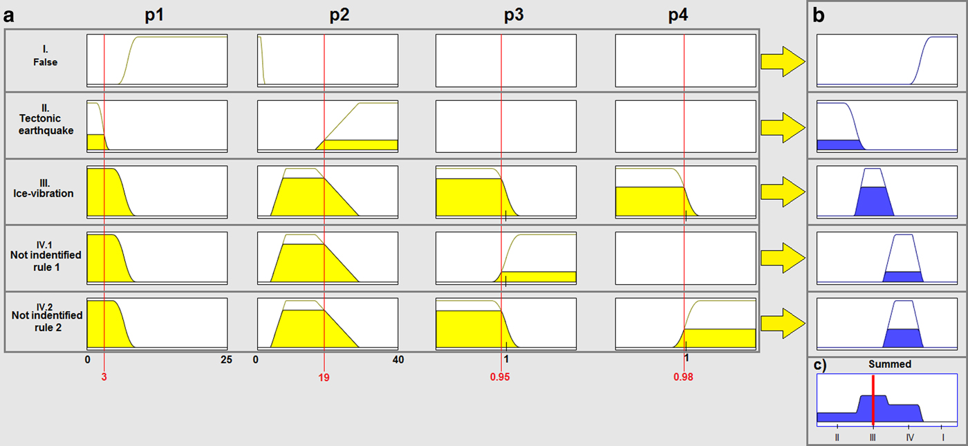
The fuzzy logic algorithm was created in MATLAB using the Fuzzy Logic Toolbox and is based on the four input parameters p i. The value of each parameter is evaluated by a membership function, which determines to what degree particular value fulfils class condition (e.g., Gaussian, which expected value is a desired one, while acceptance for deviation is expressed by standard deviation) (Fig. 3a). A sum of membership functions values for all criteria of a given class provides an assessment of the degree to which the event represents a given class (Fig. 3b). Then, the best-suited class was chosen (Fig. 3c).
A graphical representation of fuzzy logic rules evaluation in the classification algorithm. (a) The rules for each event class (False, Tectonic earthquake, Ice-vibration and two rules for Not identified) are characterised by four conditions organised into rows. Each box contains a user-defined membership function (black line) taking a particular value (from 0 to 1, vertical axis) for each possible value of the input parameter (p 1, p 2, p 3, p 4) (horizontal axis). The exemplary input parameter values are marked with thin red solid lines. The height of yellow filling in each block indicates to what degree each condition is fulfilled by exemplary input parameters. The blue lines in section are particular class membership functions (b), while blue filling height indicate to what degree this set of input parameters, p i, fulfils the rule of each respective event class (there are two rules for ‘Not identified’ – one for 6–10 and another for 11–15 Hz frequency domination). The better all four conditions are fulfilled, the better a rule is fulfilled. From the cumulative plot, (c), which is a summation of above results, the best match, a maximum (marked with a thick red solid line) in comparison with other rules can be inferred.
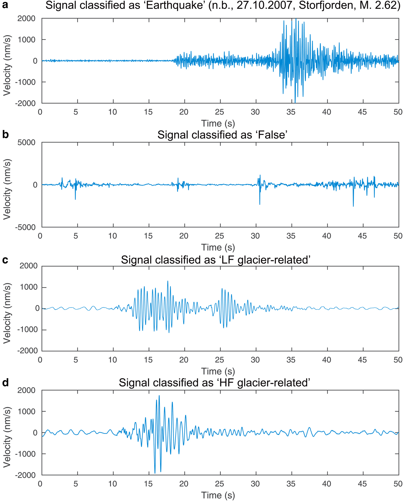
Sample waveforms representing each event class are shown in Figure 4.
Example seismograms representing each event class recorded at the HSPB station: (a) a confirmed (NORSAR earthquakes catalogue) earthquake signal with an epicentre in Storefjorden; (b) noisy detection of unknown origin; (c) signal with dominating frequency band 1–2 Hz classified as ‘Low-frequency glacier-related’; (d) signal classified as ‘High-frequency glacier-related’.
3.3. Verification of the classification algorithm
We tested the classification algorithm using a dataset kindly provided by Andreas Köhler, consisting of STA/LTA detections times at the KBS station that corresponded to visually observed calving events at Kronebreen. The data covered two periods: 14–26 August 2009 and 5–15 August 2010, and was part of the dataset that has been used in Köhler and others (Reference Köhler, Nuth, Schweitzer, Weidle and Gibbons2015). The latter period of the test dataset overlaps with dataset used in our work. Eleven out of 172 events were found in our catalogue and all of them were classified as ‘HF glacier-related’. Such a small number of detection is caused by low SNR of events in the test dataset: 83% of events has SNR < 2 (maximum amplitude divided by RMS of the whole signal filtered by 2–15 Hz bandpass filter) while SNR of all detected events was higher than 6. Detection threshold of STA/LTA algorithm used in our study was 3.
To further test the algorithm we performed our processing workflow, treating provided times as forced detections. We used test dataset consisting of 585 registrations from years 2009 and 2010. Such an approach resulted in rejection of 452 events, while 123 events were classified as follows: 1 ‘tectonic’, 8 ‘LF glacier-related’, 43 ‘HF glacier-related’ (in total 51 glacier-related), 71 ‘false’. Hence, the ratio of ‘false’ to ‘glacier-related’ was 0.72 (51/72). High number of rejected events is again caused by low SNR. Next, we decided to run only the classification algorithm using events with SNR > 2 only (102 events). The result was: 3 ‘tectonic’, 10 ‘LF glacier-related’, 38 ‘HF glacier-related’, 51 ‘false’. Hence, the ratio of ‘false’ to ‘glacier-related’ grew to 0.94 (48/51). Obtained results show that the detection threshold of the algorithm is high, because events which are detected and classified display high SNR. Lowering SNR threshold of processed events by forcing the detection resulted in increased number of events in ‘false’ group. When analysing events with high SNR, calving events from KBS tend to be classified as ‘HF glacier-related’. However, due to relatively wide frequency range of calving ice-quakes spectra, some of them were classified as ‘LF glacier-related’.
4. RESULTS
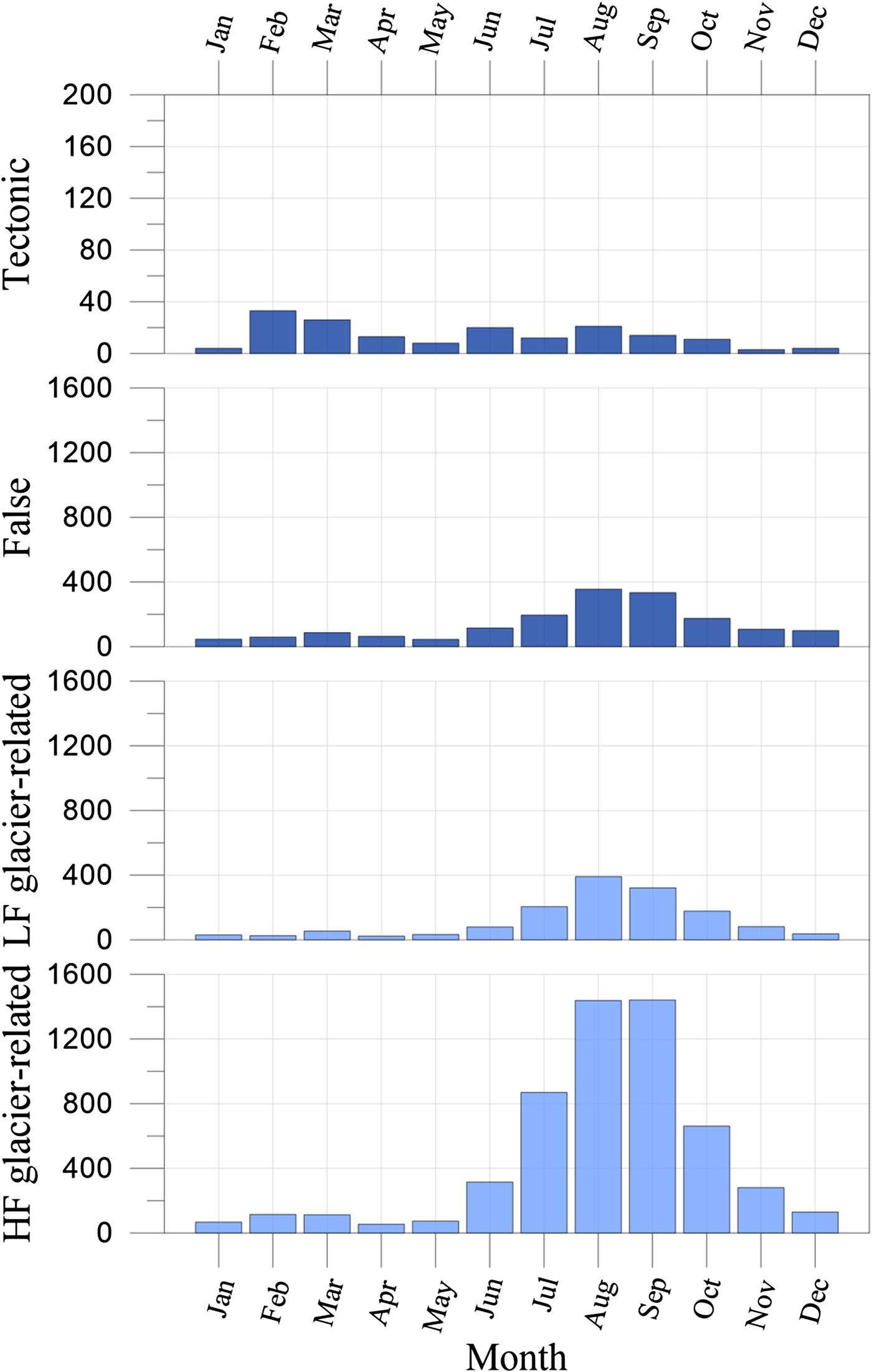
Applying our detection procedure to the continuous HSPB seismic data, we identified 8876 seismic events. Then, the fuzzy logic classification algorithm was applied. Its outcome is presented in Figure 5. There are two categories of events: ‘Tectonic’ and ‘False’, which are not glacier-induced and were therefore excluded from further analysis. Two groups remained: ‘LF glacier-related’ (1467 events) and ‘HF glacier-related’ (5553 events). Hence, 7020 detections were classified as glacier-induced (Fig. 6), while 1856 were not (grouped as ‘Tectonic’ and ‘False’).
The monthly distribution of events in each group from the HSPB station. Light blue coloured groups are affiliated with glacier-origin events. The number of events in each group are as follows: 169 ‘Tectonic’, 1687 ‘False’, 1467 ‘Low-frequency glacier-related’ and 5553 ‘High-frequency glacier-related’.
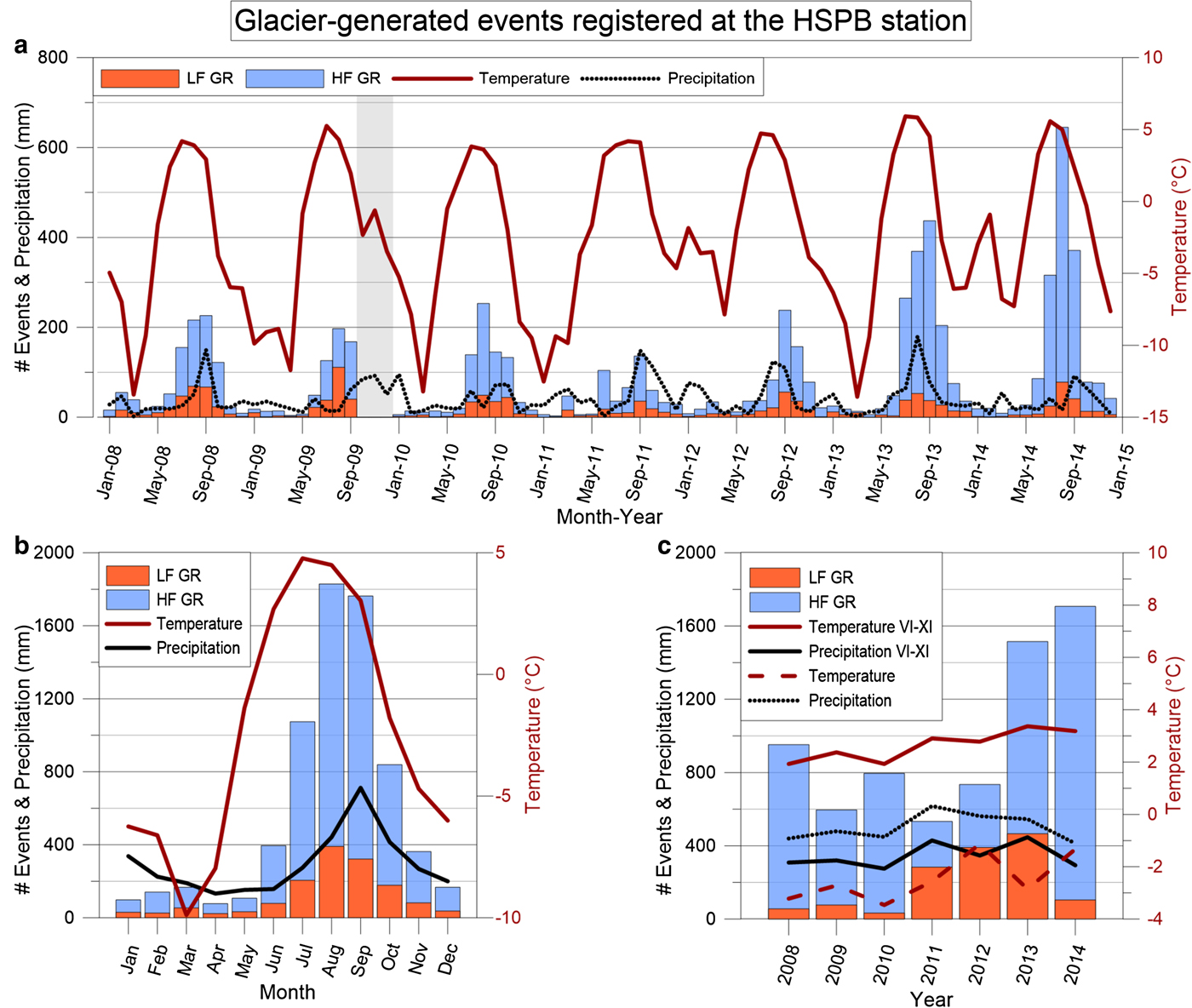
Temporal distribution of ‘glacier-induced’ events from the HSPB station. ‘Low-frequency glacier-related’ marked in orange, ‘High-frequency glacier-related’ marked in blue and plotted on top of ‘LFGR’ (a) 1 month step distribution with the mean monthly temperature – red solid line, and summed monthly precipitation – black dotted line, a data gap is indicated by the shaded rectangle; (b) monthly distribution of all events summed over 2008–2014, with summed precipitation – black solid line, and mean temperature in each month over 2008–2014 – red solid line; and (c) distribution of all events between 2008 and 2014, with the mean temperature in warm months (VI-XI) – red solid line, the summed precipitation in warm months (VI-XI) – black solid line, whole year mean temperature – red dashed line and whole year summed precipitation – black dotted line.
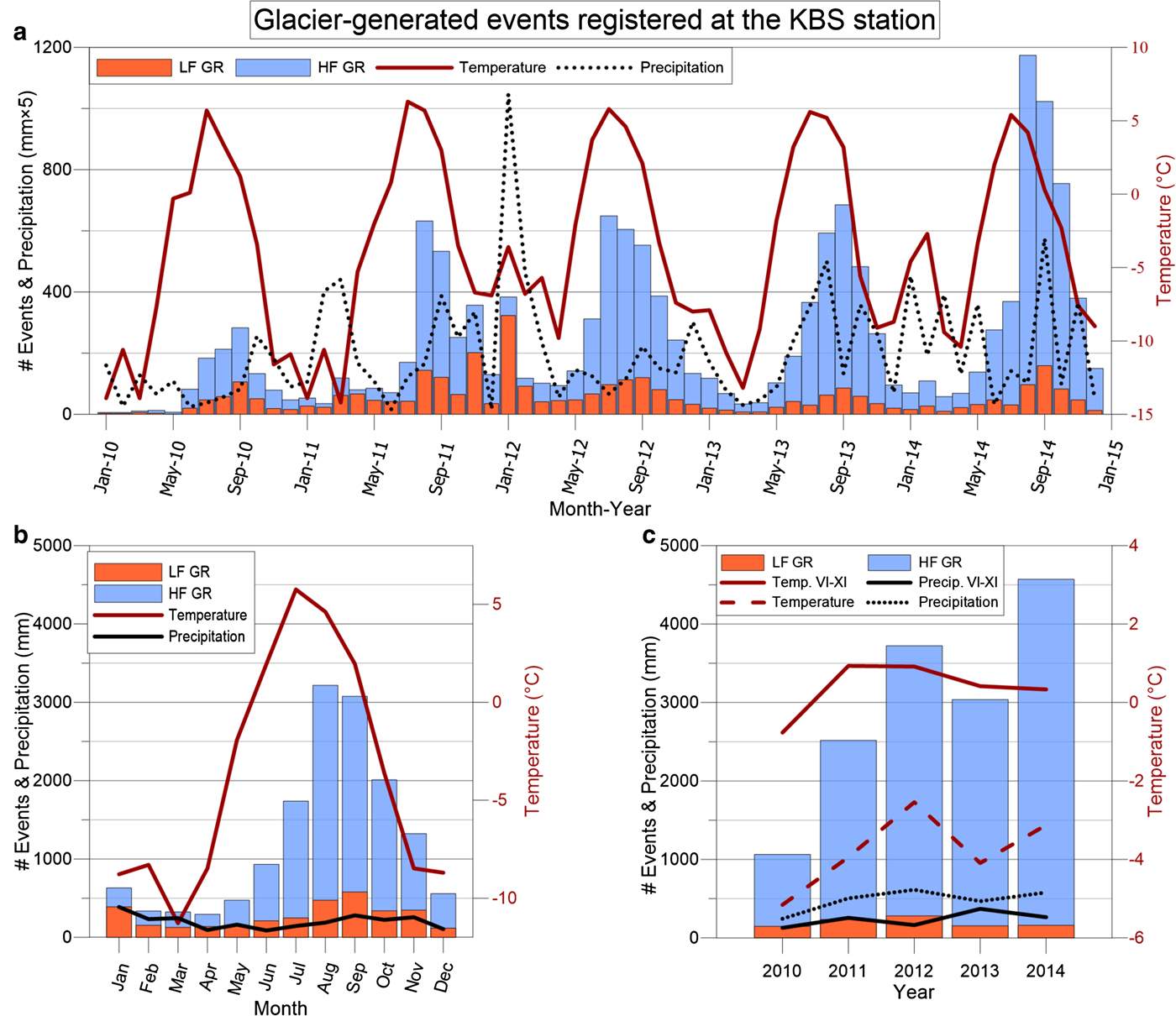
We applied the same workflow to the KBS dataset, which was recorded between 2010 and 2014, acquiring 17 711 detections then the fuzzy logic classification procedure resulted in classifying 14 913 events as glacier-related (3275 ‘LF’ and 11 638 ‘HF’) and 2798 events as tectonic or false. Figure 7 presents various distributions of those events.
Temporal distribution of ‘glacier-induced’ events from the KBS station. ‘Low-frequency glacier-related’ marked in orange, ‘High-frequency glacier-related’ marked in blue and plotted on top of ‘LFGR’ (a) 1 month step distribution with the mean monthly temperature – red solid line and summed monthly precipitation – black dotted line; (b) monthly distribution of all events summed over 2010–2014 with summed precipitation – black solid line, and mean temperature in each month over 2010–2014 – red solid line; and (c) the distribution of all events between 2010 and 2014, with the mean temperature in warm months(VI-XI) – red solid line, the summed precipitation in warm months (VI-XI) – black solid line, whole year mean temperature – red dashed line, and whole year summed precipitation – black dotted line. Note that the precipitation at panel (a) has been multiplied by 5 for better visualisation.
5. DISCUSSION
5.1. Classification
We detected several thousand events and classified them into four categories: ‘Tectonic Earthquakes’, ‘False Detections’, ‘LF glacier-related’ and ‘HF glacier-related’. The first two categories were clearly not related to a glacier and, therefore, rejected. The difference between ‘LF’ and ‘HF’ class was the domination of one of the higher frequency bands in the signal frequency spectrum, instead of the 1–5 Hz representing ‘LF’. A validation of classification criteria showed that the melt-season calving icequakes of considerable SNR are classified as ‘HF glacier-related’ much more likely than as ‘LF’, while noisy or weak calving icequakes are classified as ‘False’.
There is a significant disproportion between the obtained catalogues. Although HSPB station is situated closer to the nearest glacier, there is over two times more events detected at KSB, regardless a shorter time span. This disproportion can be explained by many factors, which have much stronger cumulative effect than the distance alone. First of all, flow rates of the glaciers differ between the two sites. Kongsbreen and Kongsvegen are among the fastest glaciers in Svalbard (Schellenberger and others, Reference Schellenberger, Dunse, Kääb, Kohler and Reijmer2015), with Kongsbreen velocity ca. 750 m a−1 (Melvold and Hagen, Reference Melvold and Hagen1998), which is over three times faster than Hansbreen (ca. 230 m a−1) (Grabiec and others, Reference Grabiec, Jania, Puczko, Kolondra and Budzik2012). Also, the width of the Kronebreen terminus is two times wider than Hansbreen's, implying a higher calving rate at Kongsfjorden. Furthermore, Kronebreen interacts with the Kongsvegen glacier (Trusel and others, Reference Trusel, Powell, Cumpston and Brigham-Grette2010), generating seismic events that are localised in the interaction zone (Koubova, Reference Koubova2015) up to 5 km from its terminus. The disproportion can also be linked with the differences in the glacier's geographical exposure to sea circulation. The ocean temperature on the western Spitsbergen coast can vary significantly, depending on the actual range of the West Spitsbergen Current (Walczowski and others, Reference Walczowski, Piechura, Goszczko and Wieczorek2012), resulting in different calving rates along the coast. Finally, the background noise level, which determines the smallest detectable events, is higher for the HSPB than for the KBS dataset.
5.2. Seasonal distribution and correlation with meteorological data
The seasonal distributions of both ‘glacier-related’ groups follow the seasonal glacier seismic activity pattern (Jania and others, Reference Jania1988; Ekström and others, Reference Ekström, Nettles and Tsai2006; Bartholomaus and others, Reference Bartholomaus2015b) and illustrate the changes in the long-term seismic activity of glaciers in the vicinity of analysed stations. Figure 6a shows the periodicity of glacier-induced events and the year-to-year changes at the HSP station. The seasonal distribution follows the same pattern each year. During winter and spring when glacier is usually advancing activity remains at the base level; then, it intensifies during the melt season from June to November, with a peak in August and September. We found this scheme to be valid for all of the analysed years, except 2011. That year, the number of ‘HF’ events in July and August is significantly lower compared with May and September. This exceptionally low number of ‘HF’ events in 2011 melt season, showing no distinct peak in August nor in September is most probably caused by a presence of dense sea-ice floes drifting in Hornsund fjord, what had drastically decreased the Hansbreen's calving intensity by cooling down surface water and suppressing waves (Pętlicki and others, Reference Pętlicki, Ciepły, Jania, Promińska and Kinnard2015). However, the distribution of ‘LF’ events is not affected severely, what is consistent with results of classification algorithm validation and suggest that ‘LF’ events sources are mainly distinct from calving icequakes.
The monthly detection distributions summed over years are shown in Figure 6b along with the mean monthly temperatures and summed precipitation curves registered at Polish Polar Station in Hornsund. We observed a 1 month delay between the temperature and ‘glacier-related’ events peak. A Pearson's correlation coefficient between the monthly ‘glacier-related’ events distribution and the mean monthly temperature equals 0.79, whereas the one calculated with a 1 month lag equals 0.85. In the case of the summed precipitation data, we obtained a correlation coefficient of 0.82 (no time lag observed).
Figure 6c presents the total number of ‘glacier-related’ events every year since 2008. It shows the mean temperature and summed precipitation during the period between June and November each year, which is the most active period of glacier seismic activity and for whole year. We noticed almost a doubling of the number of ‘HF’ events in 2013 compared with previous years, while ‘LF’ events distribution is kept stable. This high level of ‘HF’ activity was accompanied by a noticeably steady growth in the mean temperature in warm months (June–November) of 1.5°C over the analysed 7 year period. Although the correlation coefficients for the seasonal distribution were very high, they decreased severely for the year-to-year ‘glacier-related’ data suggesting that there is no correlation. Only correlation coefficient between ‘LFGR’ events and precipitation remains high: 0.78 for whole year and 0.84 for melt-season, confirming relationship between interglacial water flow and low-frequency seismic events.
Similar to the HSPB dataset, the monthly distribution of ‘glacier-related’ events near Ny-Ålesund correlates well with the number of days with mean monthly temperatures and summed precipitation measured in Ny-Ålesund (Fig. 7b), reaching the highest correlation coefficient of 0.85 (with a 1 month lag) and 0.79 (no lag) for temperatures and 0.82 for precipitation. Contrary to HSP dataset we observe high correlation coefficients for year-to-year all events distribution (Fig. 7c) with whole year summed precipitation (0.91), as well as for mean temperatures (0.88).
We observed a 1 month delay in the peak glacial seismic activity with respect to the air temperature in both datasets (Figs 6, 7). This phenomena, as well as its exceptional absence in 2012 in the Kongsfjorden region supports the theory that the sea temperature, not the air temperature, at the terminus has a key impact on the calving rate and its associated seismic signal generation (O'Leary and Christoffersen, Reference O'Leary and Christoffersen2013; Luckman and others, Reference Luckman2015; Pętlicki and others, Reference Pętlicki, Ciepły, Jania, Promińska and Kinnard2015; Truffer and Motyka, Reference Truffer and Motyka2016).
Seasonal and interannual variations in the number of glacier-related events in our study corresponded to those obtained by Köhler and others (Reference Köhler, Nuth, Schweitzer, Weidle and Gibbons2015) for the HSPB and KBS stations. Furthermore, the trend of increasing ‘glacier-related’ event numbers indicated by those authors is mutually confirmed. We have classified fewer events than Köhler and others (Reference Köhler, Nuth, Schweitzer, Weidle and Gibbons2015), which indicates that the detection criteria we used were more restrictive, what can be directly inferred from the validation test. Hence, we can assume that our detections classified as ‘HF glacier-related’ include primarily the same events as were detected by Köhler and others (Reference Köhler, Nuth, Schweitzer, Weidle and Gibbons2015).
5.3. Anomalous behaviour
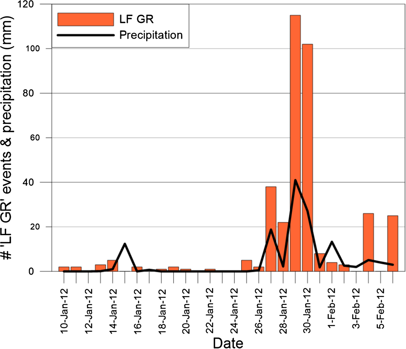
During the winter of 2011/12 temperatures higher than usual had been registered both in Hornsund and Ny-Ålesund meteorological stations. In January 2012 an extraordinary winter peak of ‘LF’ detections number was registered at KBS station, while there was no evidence of such peak at HSP station. However, the peak at KBS station clearly coincides with an extreme rain event in Kongsfjorden region (Fig. 7a). Moreover, the number of glacier-induced events is directly proportional to the precipitation (Fig. 8). Nearly all events registered between 28 and 31 January 2012 were classified as ‘LF glacier-related’ and have dominant frequencies of 1–2 Hz. There is no distinct peak in January 2012 in the study oriented to find calving events by Köhler and others (Reference Köhler, Nuth, Schweitzer, Weidle and Gibbons2015), most likely due to using higher frequency band (2–8 Hz). Schellenberger and other (Reference Schellenberger, Dunse, Kääb, Kohler and Reijmer2015) show that there was no observable increase of Kongsbreen flow in GPS velocity maps, hence the intensification of glacier seismic activity might not be connected to increased glacier flow. Registered waveforms match the characteristics of both ice-vibration (Górski and Teisseyre, Reference Górski and Teisseyre1991, Górski, Reference Górski2004) and short-duration ‘moulin’ tremor (Métaxian and others, Reference Métaxian, Araujo, Mora and Lesage2003; Röösli and others, Reference Röösli2014), caused by resonance in fluid-filled cracks, in this case due to massive rainfall, rather than to calving icequakes, what indicates connection of the interglacial water flow with the low-frequency seismic emissions.
‘Low-frequency glacier-related events’ registered at KBS station each day between 10 January 2012 and 6 February 2012 – orange bars, coinciding with extremely heavy rainfall. Summed daily precipitation – black solid line.
Observed increase in number of glacier-related events since 2011 registered at KBS station (Fig. 8a, c) agrees with observations of significantly increased ablation front in 2011–2013 of both Kronebreen and Kongsbreen (Schellenberger and others, Reference Schellenberger, Dunse, Kääb, Kohler and Reijmer2015).
5.4. Periodicity
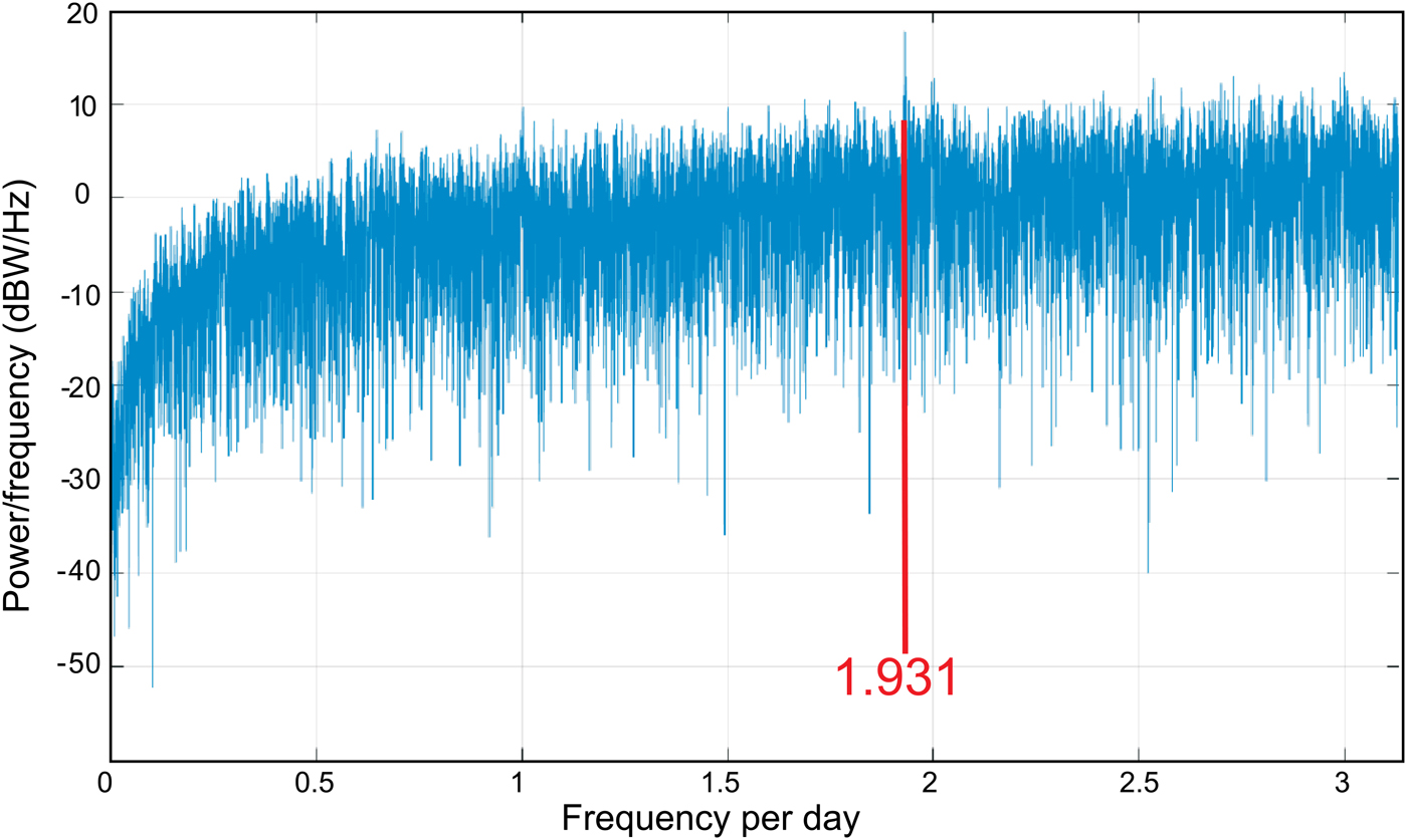
Bartholomaus and others (Reference Bartholomaus2015b) claim that the periodicity of iceberg calving coincides with principal lunar semidiurnal tide. Following this work, we decided to analyse periodicity of detected ‘glacier-related’ events. We summed glacier-induced detection times in short-duration bins (3.83 h) and then computed the Lomb-Scargle periodogram, which is suitable for power spectra representation for irregularly spaced data (Press and others, Reference Press, Flannery, Teukolsky and Vetterling1992). For KBS dataset we recognised a distinct peak at 0.5179 d (1/1.931 d) coinciding with the principal lunar semidiurnal tide (K 1 = 0.5175 d (1/1.932)) (Fig. 9), same as Bartholomaus and others (Reference Bartholomaus2015b) found for the Yahtse glacier. There was no evidence for this peak at HSP dataset, which we believe is caused by too sparse time coverage of events and lower calving rate. Recognised peak can support a connection between variations in sea level and increased calving showed already by only two authors (O'Neel and others, Reference O'Neel, Echelmeyer and Motyka2003; Bartholomaus and others, Reference Bartholomaus2015b).
Power spectrum of ‘glacier-related’ seismic events detection times at KBS station calculated by applying the Lomb-Scargle algorithm to the demeaned, detrended detection times distribution in 3.83 h bins. The frequency peak of 1.931 d−1 corresponding to K1 principal lunar semidiurnal tide (1.932 d−1) is labelled.
5.5. Algorithm's performance
The developed algorithm was implemented on a PC desktop computer, which was able to process a few yearlong continuous datasets within 1 d. Thus, this approach can be easily implemented as a routine tool for real- or near-real-time glacier activity monitoring. The parameterisation of the grouping conditions of the fuzzy logic algorithm might differ for various datasets because of different factors such as the noise level, distance to the sources in a glacier or characteristics of background noise, however, after initial inspection of the detected signals, the chosen thresholds and parameters can be adjusted.
The performance of our method can be significantly improved by using more than one station, which would allow for the assessment of event locations, which are hardly possible to obtain using a single station (Asming and Fedorov, Reference Asming and Fedorov2015). Without a location assessment, we cannot reliably affiliate the detected seismicity with any particular glacier. Consequently, we affiliate them with the station area, i.e., with the largest ice masses surrounding the station. On the other hand, presented method can be applied if there is only a single station available in the area.
6. CONCLUSIONS
We developed an automatic algorithm to detect glacier-related seismic events using the continuous seismic records of a single seismic station. Using fuzzy logic, our algorithm classifies detections as glacier-related or non-glacier-related.
We used recordings from two broadband seismological stations, HSPB in southern Spitsbergen and KBS in western Spitsbergen, to analyse glacial dynamic activity near the Hansbreen and Kronebreen glaciers. We detected and classified more than 8000 events over a 7 year time span (2008–2014) in the HSPB station region, classifying 7020 of them as glacier induced. We also detected more than 17000 events throughout a 5 year time span (2010–2014) for the KBS dataset, with 14 913 of them classified as glacier-induced.
In recent years, the number of detected glacier-related events in the analysed regions of Spitsbergen increased significantly. In the HSPB dataset, they doubled over the last 2 years (2013/14), whereas in the KBS dataset, a steady increase from year to year was observed.
The cumulative seasonal event distribution correlates well with the seasonal temperature variations. The highest correlation coefficients (0.95 and 0.96) were observed between the glacier seismic activity and the number of days with positive mean temperatures delayed by 1 month for both datasets. Correlation coefficients with 1 month delayed mean temperatures and summed precipitation were also high. A year-to-year cumulative event distribution revealed much weaker correlations with meteorological data or no correlations at all.
Weather phenomena like, for example extreme rainfall can distinctly contribute to the seasonal distribution of glacier-induced seismic events, as observed in January 2012 in Kongsfjorden. Distribution of the rainfall-triggered events is dominated by the low-frequency events rather than typical calving events. Hence, the group of ‘LF glacial-related’ events should instead be affiliated with the internal processes within a glacier, like interglacial water flow.
Large cover of floating ice can efficiently decrease calving intensity throughout whole melt season, as happened in 2011 in Hornsund. Results from Kongsfjorden seem to confirm the idea that the principal lunar semidiurnal tide can contribute significantly to calving periodicity.
Our results demonstrate the possibility of using long-term seismological observations from a single permanent seismic station to study the dynamic activity of glaciers located in their proximity. The time-efficient automatic event detection and classification algorithm based on fuzzy logic can be used to discriminate automatically and objectively between non-glacier and glacier-related events in real time, revealing temporal changes and long-term trends in glacier dynamics.
ACKNOWLEDGEMENTS
The HSPB seismological station is operated by the Institute of Geophysics, Polish Academy of Sciences, in cooperation with the NORSAR research foundation. It was installed within the framework of an IPY project, mainly financed by the Research Council of Norway (contract no. 176069/S30) and is part of the Polish Seismological Network. The KBS seismological station belongs to the Norwegian Seismological Network and is maintained by the University of Bergen. We thank Andreas Köhler for sharing the Kronebreen calving event catalog, which allowed us to validate the classification algorithm. We would like to thank Tomasz Wawrzyniak and the Hornsund Polish Polar Station staff for establishing and maintaining the Hornsund GLACIO-TOPOCLIM database used in this investigation. We would also like to acknowledge the Norwegian Meteorological Institute for establishing and maintaining the free access weather and climate data eKlima service that was used for this research. The seismological records were downloaded from free online databases of IRIS and Orfeus. This work was partially supported within the statutory activities No 3841/E-41/S/2016 of the Ministry of Science and Higher Education of Poland. We also thank two anonymous reviewers and the scientific editor for their comments that helped us improve the manuscript. The publication has been partially financed from the funds of the Leading National Research Centre (KNOW) received by the Centre for Polar Studies for the period 2014–2018.


 Open access