

1 INTRODUCTION
Circumstellar disks are formed around protostars during the gravitational collapse of molecular cloud core. Because the disks are the formation sites of planets, the formation and evolution processes of the disk essentially determine the initial conditions for planet formation. Hence, understanding disk formation and evolution is crucial for constructing a comprehensive theory for planet formation. An accurate description of the angular momentum evolution is required to investigate the disk evolution because the centrifugal force mainly balances the gravitational force of the central protostar.
Formation of a circumstellar disk around a very young protostar had been believed to be a natural consequence of angular momentum conservation in the gravitationally collapsing molecular cloud core. Observations of cloud cores have shown that they have finite angular momentum (e.g., Goodman et al. Reference Goodman, Benson, Fuller and Myers1993; Caselli et al. Reference Caselli, Benson, Myers and Tafalla2002).
Many studies of the cloud core collapse without a magnetic field have been conducted (Boss & Bodenheimer Reference Boss and Bodenheimer1979; Bate Reference Bate1998; Truelove et al. Reference Truelove, Klein, McKee, Holliman, Howell, Greenough and Woods1998; Matsumoto & Hanawa Reference Matsumoto and Hanawa2003; Commerçon et al. Reference Commerçon, Hennebelle, Audit, Chabrier and Teyssier2008; Attwood et al. Reference Attwood, Goodwin, Stamatellos and Whitworth2009; Walch et al. Reference Walch, Burkert, Whitworth, Naab and Gritschneder2009; Machida, Inutsuka, & Matsumoto Reference Machida, Inutsuka and Matsumoto2010; Stamatellos, Whitworth, & Hubber Reference Stamatellos, Whitworth and Hubber2012; Walch, Whitworth, & Girichidis Reference Walch, Whitworth and Girichidis2012; Tsukamoto & Machida Reference Tsukamoto and Machida2013; Tsukamoto, Machida, & Inutsuka Reference Tsukamoto, Machida and Inutsuka2013), and it is now well established that a relatively large disk with a size of r ~ 100 AU is formed during the early phase of protostar formation and fragmentation also occurs in the unmagnetised cores.
However, the magnetic field changes this simple process of disk formation. During the gravitational collapse, a toroidal magnetic field is created and the magnetic tension decelerates the gas rotation, removing the angular momentum. This process is known as magnetic braking. Its importance in circumstellar disk formation was recognised in the past decade, although there had been several theoretical studies regarding magnetic braking (Gillis, Mestel, & Paris Reference Gillis, Mestel and Paris1974, Reference Gillis, Mestel and Paris1979; Mouschovias & Paleologou Reference Mouschovias and Paleologou1979, Reference Mouschovias and Paleologou1980), focusing mostly on the angular momentum evolution of molecular clouds or cores. Simulations in which the ideal magnetohydrodynamics (MHD) approximation is adopted and the magnetic field is aligned with the rotation vector have shown that disk formation is almost completely suppressed in moderately magnetised cloud cores by magnetic braking (Allen, Li, & Shu Reference Allen, Li and Shu2003; Price & Bate Reference Price and Bate2007b; Mellon & Li Reference Mellon and Li2008; Hennebelle & Fromang Reference Hennebelle and Fromang2008).
Several mechanisms have been suggested to reduce the magnetic braking efficiency. For example, misalignment between the magnetic field and the rotation vector and turbulence are suggested as mechanisms that weaken magnetic braking in the ideal MHD limit (Hennebelle & Ciardi Reference Hennebelle and Ciardi2009; Joos, Hennebelle, & Ciardi Reference Joos, Hennebelle and Ciardi2012; Santos-Lima, de Gouveia Dal Pino, & Lazarian Reference Santos-Lima, de Gouveia Dal Pino and Lazarian2012; Seifried et al. Reference Seifried, Banerjee, Pudritz and Klessen2013; Joos et al. Reference Joos, Hennebelle, Ciardi and Fromang2013; Li, Krasnopolsky, & Shang Reference Li, Krasnopolsky and Shang2013). Non-ideal effects (Ohmic diffusion, the Hall effect, and ambipolar diffusion), which arise from the finite conductivity in the cloud core, also serve as mechanisms that change the magnetic braking efficiency (Duffin & Pudritz Reference Duffin and Pudritz2009; Machida & Matsumoto Reference Machida and Matsumoto2011; Krasnopolsky, Li, & Shang Reference Krasnopolsky, Li and Shang2011; Li, Krasnopolsky, & Shang Reference Li, Krasnopolsky and Shang2011; Tomida et al. Reference Tomida, Tomisaka, Matsumoto, Hori, Okuzumi, Machida and Saigo2013; Tomida, Okuzumi, & Machida Reference Tomida, Okuzumi and Machida2015; Tsukamoto et al. Reference Tsukamoto, Iwasaki, Okuzumi and Machida2015b; Masson et al. Reference Masson, Chabrier, Hennebelle, Vaytet and Commerçon2015; Tsukamoto et al. Reference Tsukamoto, Iwasaki, Okuzumi and Machida2015a).
In this paper, we review recent progress on the influence of the magnetic field on the formation and early evolution of the circumstellar disk. The paper is organised as follows. We review the observed properties of cloud cores in Section 2 and summarise gravitational collapse of cloud cores in Section 3. The main part of this paper, Sections 4 to 6, covers recent studies of disk formation and early evolution in magnetised cloud cores. In Section 7, we summarise our current understanding of disk formation and early evolution, and discuss future perspectives.
2 OBSERVATIONAL PROPERTIES OF MOLECULAR CLOUD CORES
In this section, we give an overview of the observational properties of molecular cloud cores.
2.1 Rotation of the cores
An important parameter of the cloud core is its rotation energy. Rotation of cloud cores is often observationally measured using the velocity gradient obtained from the NH3 (1,1) inversion transition line or N2H+ (1 − 0) rotational transition line (Goodman et al. Reference Goodman, Benson, Fuller and Myers1993; Barranco & Goodman Reference Barranco and Goodman1998; Caselli et al. Reference Caselli, Benson, Myers and Tafalla2002; Pirogov et al. Reference Pirogov, Zinchenko, Caselli and Johansson2003). On the other hand, simulations of cloud core formation are performed to theoretically investigate core rotation (Offner, Klein, & McKee Reference Offner, Klein and McKee2008; Dib et al. Reference Dib, Hennebelle, Pineda, Csengeri, Bontemps, Audit and Goodman2010). Figure 1 shows the histograms of βrot ≡ E rot/E grav from Dib et al. (Reference Dib, Hennebelle, Pineda, Csengeri, Bontemps, Audit and Goodman2010), where E rot and E grav are the rotational and gravitational energy of the core, respectively. In this figure, both the observation (black dotted lines) and simulation results (coloured lines) are plotted. The peaks of both lines show that the cores typically have a βrot value of ~ 0.01. Hence, both the observations and the simulations suggest that the rotational energy of a typical cloud core is about 1% of its gravitational energy.
Histogram of βrot( ≡ E rot/E grav) of cloud cores obtained using the simulations of Dib et al. (Reference Dib, Hennebelle, Pineda, Csengeri, Bontemps, Audit and Goodman2010) (coloured lines) and observations of Goodman et al. (Reference Goodman, Benson, Fuller and Myers1993), Barranco & Goodman (Reference Barranco and Goodman1998), and Caselli et al. (Reference Caselli, Benson, Myers and Tafalla2002) (black lines). This figure appears as Figure 6 of Dib et al. (Reference Dib, Hennebelle, Pineda, Csengeri, Bontemps, Audit and Goodman2010). Coloured lines in the upper panels show βrot with a low density threshold for n th = 2.0 × 104 cm− 3, whereas, those in the lower panels show βrot with a high density threshold for n th = 8.0 × 104 cm− 3. The low and high density thresholds correspond roughly to the excitation density for the NH3 (J − K)=(1,1) transition and the N2H+ (1 − 0) emission lines, respectively. The observational results obtained for the NH3 (J − K)=(1,1) transition (upper panels) and the N2H+ (1 − 0) emission line (lower panels) are plotted with black-dashed lines. The NH3 core observations are from Goodman et al. (Reference Goodman, Benson, Fuller and Myers1993) and Barranco & Goodman (Reference Barranco and Goodman1998) and the N2H+ data are from Caselli et al. (Reference Caselli, Benson, Myers and Tafalla2002). The left and right panels show the results with strong and weak initial magnetic fields. The initial plasma β in the left and right panels are β = 0.1 and β = 1, respectively.

2.2 Turbulence in the cores
The molecular cloud has a complex internal velocity structure over a wide range of scales that is interpreted as turbulent motion (Larson Reference Larson1981) and, even at the cloud core scale, there exist non-thermal motions (Barranco & Goodman Reference Barranco and Goodman1998). Burkert & Bodenheimer (Reference Burkert and Bodenheimer2000) showed that a random Gaussian velocity field with P(k)∝k − 4 can explain the observed rotational properties of the cores. Note that P(k)∝k − 4 is very similar to the Kolmogorov spectrum P(k)∝k − 11/3. Thus, it is expected that turbulence exists in cloud cores although coherent rotation is often assumed in the theoretical study of the cloud core collapse (e.g., Bate Reference Bate1998; Matsumoto & Hanawa Reference Matsumoto and Hanawa2003; Walch et al. Reference Walch, Burkert, Whitworth, Naab and Gritschneder2009; Tsukamoto & Machida Reference Tsukamoto and Machida2011). The turbulent velocity inside the cores is typically subsonic (Ward-Thompson et al. Reference Ward-Thompson, André, Crutcher, Johnstone, Onishi and Wilson2007).
2.3 Magnetic field in the core
Another important physical quantity is the strength of the magnetic field. The strength of the magnetic field is often expressed using the mass-to-flux ratio relative to the critical mass-to-flux ratio (Mouschovias & Spitzer Reference Mouschovias and Spitzer1976),
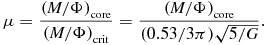 $$\begin{eqnarray}
\mu =\frac{(M/\Phi )_{\rm core}}{(M/\Phi )_{\rm crit}}=\frac{(M/\Phi )_{\rm core}}{(0.53/3\pi ) \sqrt{5/G}}.
\end{eqnarray}$$
$$\begin{eqnarray}
\mu =\frac{(M/\Phi )_{\rm core}}{(M/\Phi )_{\rm crit}}=\frac{(M/\Phi )_{\rm core}}{(0.53/3\pi ) \sqrt{5/G}}.
\end{eqnarray}$$
When μ < 1, the magnetic pressure is strong enough to support the cloud core against its self-gravity. The critical value,
 $(M/\Phi )_{\rm crit}=0.53/3\pi \sqrt{5/G}$
is derived for a spherically symmetric cloud core. This critical value is often used in theoretical study. Another critical mass-to-flux ratio is derived for the stability of disks and expressed as (Nakano & Nakamura Reference Nakano and Nakamura1978),
$(M/\Phi )_{\rm crit}=0.53/3\pi \sqrt{5/G}$
is derived for a spherically symmetric cloud core. This critical value is often used in theoretical study. Another critical mass-to-flux ratio is derived for the stability of disks and expressed as (Nakano & Nakamura Reference Nakano and Nakamura1978),
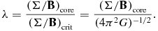 $$\begin{eqnarray}
\lambda =\frac{(\Sigma /\boldsymbol{B})_{\rm core}}{(\Sigma /\boldsymbol{B})_{\rm crit}}=\frac{(\Sigma /\boldsymbol{B})_{\rm core}}{(4\pi ^2 G)^{-1/2}}.
\end{eqnarray}$$
$$\begin{eqnarray}
\lambda =\frac{(\Sigma /\boldsymbol{B})_{\rm core}}{(\Sigma /\boldsymbol{B})_{\rm crit}}=\frac{(\Sigma /\boldsymbol{B})_{\rm core}}{(4\pi ^2 G)^{-1/2}}.
\end{eqnarray}$$
This is often used in observational study.
The magnetic field strength of the molecular clouds and cores can be measured using the Zeeman effect (Crutcher et al. Reference Crutcher, Troland, Goodman, Heiles, Kazes and Myers1993, Reference Crutcher, Troland, Lazareff and Kazes1996; Falgarone et al. Reference Falgarone, Troland, Crutcher and Paubert2008; Troland & Crutcher Reference Troland and Crutcher2008; Crutcher Reference Crutcher2012). Figure 2 shows the observation of the magnetic field of the cloud cores using the OH Zeeman effect. This figure appears as Figure 2 of Troland & Crutcher (Reference Troland and Crutcher2008). They found that the mean value of the mass-to-flux ratio of the observed cloud cores is λobs = 4.8 ± 0.4. By applying a geometrical correction, they showed that the mean mass-to-flux ratio of the cloud cores is λ ~ 2. Hence, most cores are supercritical, meaning that the magnetic field is not strong enough to support the cloud core by magnetic pressure. However, the energy of the magnetic field in cores with λ ~ 2 could be several tens of percent of its gravitational energy, which is much larger than the rotation velocity. Therefore, the magnetic field is expected to affect the gas dynamics during gravitational collapse.
Observed line-of-sight magnetic field strength B los plotted as a function of the H2 column density [N 21 = 10− 21 n(cm− 2)]. This figure appears as Figure 2 of Troland & Crutcher (Reference Troland and Crutcher2008). Error bars indicate 1σ. The mass-to-flux ratio normalised by the critical value is given as λ = 7.6 × 10− 21 N 21/B los. The solid line represents the weighted mean value for the mass-to-flux ratio λ = 4.8 ± 0.4, whereas the dashed line represents the value for λ = 1.

3 GRAVITATIONAL COLLAPSE OF CLOUD CORE
In this section, we discuss gravitational collapse of molecular cloud cores. Some terminology is also introduced in this section.
Once the core becomes massive enough and gravitationally unstable, dynamical collapse of the cloud core begins. At the beginning of the collapse, radiation cooling by dust thermal emission is sufficiently effective, and the gas temperature remains almost isothermal at a temperature T = 10 K. During this isothermal collapse phase, the magnetic field is essentially frozen into the gas. When the Lorentz force is weak and negligible, the collapse can be described well as spherically symmetric collapse. Larson (Reference Larson1969) has shown that the isothermal gravitational collapse proceeds self-similarly. As a result, the density profile in the isothermal collapse phase has a central flat profile; the radius is characterised by the Jeans length λJ and the outer envelope has ρ∝r − 2, as shown in Larson (Reference Larson1969). In the spherically symmetric collapse phase, the magnetic field evolves as B∝ρ2/3.
As the isothermal spherical collapse proceeds, the magnetic field is amplified, and the plasma β ≡ P gas/P mag) decreases as β∝ρ− 1/3, where P gas and P mag are the gas and magnetic pressure, respectively. Hence, at some point, the Lorentz force becomes effective and begins to deflect the gas motion toward the direction parallel to the magnetic field. This breaks the spherically symmetric collapse. The gas density increases by the parallel accretion, while the magnetic field strength remains almost constant.
As a result of parallel accretion, the gas moves to the equatorial plane, forming a sheet-like structure known as a pseudodisk (Galli & Shu Reference Galli and Shu1993). Figure 3 shows the density map of the pseudodisk formed in the simulation of Tsukamoto et al. (Reference Tsukamoto, Iwasaki, Okuzumi and Machida2015a), for example. Its radius is typically r ≳ 100 AU at the protostar formation epoch. Because of the inward dragging of the magnetic field, the magnetic field configuration exhibits an hourglass shape (Tomisaka, Ikeuchi, & Nakamura Reference Tomisaka, Ikeuchi and Nakamura1988a; Galli & Shu Reference Galli and Shu1993) and a current sheet exists at its midplane. The hourglass shape of the magnetic field is also inferred from observations (Girart, Rao, & Marrone Reference Girart, Rao and Marrone2006; Cortes & Crutcher Reference Cortes and Crutcher2006; Gonçalves, Galli, & Girart Reference Gonçalves, Galli and Girart2008). The figure also shows that the velocity is almost parallel to the magnetic field except around the midplane indicating that the gas moves parallel to the magnetic field. Note that the pseudodisk is not rotationally supported although its morphology is disk-like.
Density structure of the pseudodisk in x–z plane. This figure is obtained using simulation results in which all of the non-ideal effects are considered and the magnetic field and rotation vector are parallel. The simulation corresponds to model Ortho defined in Tsukamoto et al. (Reference Tsukamoto, Iwasaki, Okuzumi and Machida2015a) and the simulation setup is described in detail in the paper. At this epoch, the central protostar is formed. The red and white arrows indicate the velocity field and direction of the magnetic field, respectively.

The gas continues to accrete toward the central region mainly through the pseudodisk. If the disk-like structure is maintained, the magnetic field increases as B
c∝ρ1/2
c because the central magnetic field and density evolve as B
c∝R
− 2 and ρc∝R
− 2
H
− 1∝R
− 4, respectively, and hence B
c∝ρ1/2
c. Here, we assumed that the scale-height of the pseudodisk is given by
 $H_{\rm c}=c_{\rm s}^2/(G \Sigma )=c_{\rm s}/\sqrt{G \rho _{\rm c}}$
.
$H_{\rm c}=c_{\rm s}^2/(G \Sigma )=c_{\rm s}/\sqrt{G \rho _{\rm c}}$
.
When the central density reaches ρ ~ 10− 13g cm− 3, compressional heating overtakes radiative cooling, and the gas begins to evolve adiabatically. As a result, gravitational collapse temporarily stops and a quasi-hydrostatic core, commonly known as the first core or the adiabatic core, forms (Larson Reference Larson1969; Masunaga & Inutsuka Reference Masunaga and Inutsuka1999; Vaytet et al. Reference Vaytet, Audit, Chabrier, Commerçon and Masson2012, Reference Vaytet, Chabrier, Audit, Commerçon, Masson, Ferguson and Delahaye2013). In cores with very weak or no magnetic field, a disk several tens of AU in size can form around first core before protostar formation (Bate Reference Bate1998; Matsumoto & Hanawa Reference Matsumoto and Hanawa2003; Walch et al. Reference Walch, Burkert, Whitworth, Naab and Gritschneder2009; Tsukamoto & Machida Reference Tsukamoto and Machida2011; Tsukamoto et al. Reference Tsukamoto, Takahashi, Machida and Inutsuka2015c). In the first core phase, the temperature evolves as T∝ργ − 1, where γ is the adiabatic index (γ = 5/3 for T ≲ 100 K, and γ = 7/5 for 100 ≲ T ≲ 2000 K). As we will discuss below, in the first core, magnetic diffusion becomes effective, and the gas and the magnetic field are temporarily decoupled until the central temperature reaches ~ 1000 K, and thermal ionisation provides sufficient ionisation.
When the central temperature of the first core reaches ~ 2000 K, the hydrogen molecules begin to dissociate. This endothermic reaction changes the effective adiabatic index to γeff = 1.1, and gravitational collapse resumes, which is known as the second collapse. Finally, when the molecular hydrogen is completely dissociated, the gas evolves adiabatically again, and gravitational collapse at the centre finishes. The adiabatic core formed at the centre is the protostar (or the second core). After the protostar forms, it evolves by mass accretion from the envelope (the remnant of the host cloud core), and, at some point, a circumstellar disk is formed around the protostar.
4 MAGNETIC BRAKING AND SUPPRESSION OF DISK FORMATION
In this section, we review angular momentum transfer by the magnetic field, focusing in particular on magnetic braking. We investigate the most simple case, in which the ideal MHD approximation is adopted, the magnetic field and rotation axis are parallel, and the core rotation is coherent. The effects of misalignment and turbulence are discussed in Section 5 and the effects of non-ideal MHD effect are discussed in Section 6.
4.1. Timescale of magnetic braking
An estimate of the magnetic braking timescale would be useful for understanding the basic characteristics of magnetic braking. As shown in many previous studies (Mouschovias & Paleologou Reference Mouschovias and Paleologou1979, Reference Mouschovias and Paleologou1980; Mouschovias Reference Mouschovias1985; Nakano Reference Nakano1989; Tomisaka, Ikeuchi, & Nakamura Reference Tomisaka, Ikeuchi and Nakamura1990), the magnetic braking timescale t b can be estimated as the time in which the torsional Alfvén waves sweep an amount of gas in the outer envelope for which the moment of inertia I ext(t b) equals that of the central region I c. This condition is expressed as
 $$\begin{eqnarray}
I_{\rm ext}(t_{\rm b})=I_{\rm c}.
\end{eqnarray}$$
$$\begin{eqnarray}
I_{\rm ext}(t_{\rm b})=I_{\rm c}.
\end{eqnarray}$$
By solving this equation for a specified geometry of the central region and outer envelope, we can obtain the magnetic braking timescale.
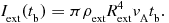
In the simplest geometry, the central collapsing region is modelled as a uniform cylinder with a density ρc, radius R c, and scale height H c threaded by a uniform magnetic field parallel to the rotation axis. The density of the outer envelope, ρext is assumed to be constant. In this geometry, I ext(t b) = πρext R 4 c v A t b and I c = πρc R 4 c H c, where v A denotes the Alfvén velocity of the outer envelope. Thus, t b is given as (Mouschovias Reference Mouschovias1985)
 $$\begin{eqnarray}
t_{\rm b}=\frac{\rho _{\rm c}}{\rho _{\rm ext}}\frac{H_{\rm c}}{v_{\rm A}}.
\end{eqnarray}$$
$$\begin{eqnarray}
t_{\rm b}=\frac{\rho _{\rm c}}{\rho _{\rm ext}}\frac{H_{\rm c}}{v_{\rm A}}.
\end{eqnarray}$$
Using the mass of the cylinder, M = 2πρc R 2 c H c, and the magnetic flux Φ = πR 2 c B, we can rewrite Equation (4) as
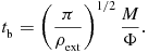 $$\begin{eqnarray}
t_{\rm b} = \left( \frac{\pi }{\rho _{\rm ext}} \right)^{1/2} \frac{M}{\Phi }.
\end{eqnarray}$$
$$\begin{eqnarray}
t_{\rm b} = \left( \frac{\pi }{\rho _{\rm ext}} \right)^{1/2} \frac{M}{\Phi }.
\end{eqnarray}$$
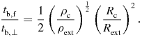
This shows that the magnetic braking timescale in this simple geometry is determined only by the mass-to-flux ratio of the central region and the density of the outer envelope. This timescale can be regarded as the upper limit in the collapsing cloud core because, as shown in Figure 3, the magnetic field has an hourglass shape in the gravitationally collapsing cloud core. In this more realistic configuration, the correction factor ( < 1) resulting from the magnetic field geometry is multiplied by the braking timescale.
As illustrated schematically in Figure 4, in the hourglass configuration, the magnetic field fans out in the vertical direction. If we neglect the moment of inertia of the transitional region, I ext(t b) is given as
 $$\begin{eqnarray}
I_{\rm ext}(t_{\rm b})=\pi \rho _{\rm ext} R_{\rm ext}^4 v_{\rm A} t_{\rm b}.
\end{eqnarray}$$
$$\begin{eqnarray}
I_{\rm ext}(t_{\rm b})=\pi \rho _{\rm ext} R_{\rm ext}^4 v_{\rm A} t_{\rm b}.
\end{eqnarray}$$
Using I c = πρc R 4 c H c and Equation (6), we can obtain the magnetic braking timescale of the disk with hourglass magnetic field geometry as (Mouschovias Reference Mouschovias1985)
 $$\begin{eqnarray}
t_{\rm b,f}=\left( \frac{\pi }{\rho _{\rm ext}} \right)^{1/2} \left(\frac{M}{\Phi }\right) \left(\frac{R_{\rm c}}{R_{\rm ext}}\right)^2.
\end{eqnarray}$$
$$\begin{eqnarray}
t_{\rm b,f}=\left( \frac{\pi }{\rho _{\rm ext}} \right)^{1/2} \left(\frac{M}{\Phi }\right) \left(\frac{R_{\rm c}}{R_{\rm ext}}\right)^2.
\end{eqnarray}$$
Here, we assume that R ext = (B c/B ext)1/2 R c because of the conservation of the magnetic flux. This shows that the magnetic braking timescale could become much shorter than t b in Equation (5) because (R c/R ext) < 1.
Schematic figure of the geometry assumed in the derivation of Equations (6) and (7). R c, H c, and ρc are the radius, scale height, and density of the central cylinder, respectively. R ext, ρext are the radius of flux-tube and density of outer envelope, respectively.

The ratio of the radii, (R c/R ext) is highly uncertain. Furthermore, the density structure of the envelope evolves with time. These uncertainties make the analytical treatment of magnetic braking difficult (see, however, Nakano Reference Nakano1989; Tomisaka et al. Reference Tomisaka, Ikeuchi and Nakamura1990; Krasnopolsky & Königl Reference Krasnopolsky and Königl2002; Dapp & Basu Reference Dapp and Basu2010; Dapp, Basu, & Kunz Reference Dapp, Basu and Kunz2012, for example). Therefore, multidimensional simulation of the collapsing cloud core is an important tool for investigating the effect of magnetic braking in a realistic magnetic field configuration.
4.2. Numerical simulations of magnetic braking
Using a two-dimensional ideal MHD simulation starting from cylindrical isothermal cloud cores, Tomisaka (Reference Tomisaka2000) clearly showed that much of the angular momentum is removed from the central region by magnetic braking and outflow. He showed that about two-thirds of the initial specific angular momentum is removed from the central region during the runaway collapse phase, and more is removed after the formation of the first core by outflow and magnetic braking. At the end of the simulation, most of the specific angular momentum has been removed from the central region (a reduction of 104 from the initial value). His simulation clearly indicates the importance of angular momentum transfer by the magnetic field.
Allen et al. (Reference Allen, Li and Shu2003) showed that magnetic braking in the main accretion phase is significant and that much of the angular momentum is removed from the accreting gas using two-dimensional ideal MHD simulations starting from singular isothermal toroids. They pointed out that the magnetic braking efficiency is enhanced by hourglass like magnetic field geometry around the pseudodisk because the magnetic field is strengthened and the reduction factor (R c/R ext)2 in the timescale of Equation (7) becomes small. Because of the two enhancement mechanisms for magnetic braking in the pseudodisk, magnetic braking plays an important role in the angular momentum evolution of accreting gas. Note that most of the gas accretes onto the central star through the pseudodisk, and angular momentum removal in the pseudodisk strongly affects formation and evolution of the circumstellar disk around the protostar.
This significant removal of angular momentum in the ideal MHD limit was later confirmed using two- or three-dimensional simulations (Banerjee & Pudritz Reference Banerjee and Pudritz2006; Price & Bate Reference Price and Bate2007b; Hennebelle & Fromang Reference Hennebelle and Fromang2008; Mellon & Li Reference Mellon and Li2008; Machida et al. Reference Machida, Inutsuka and Matsumoto2011b; Bate, Tricco, & Price Reference Bate, Tricco and Price2014). These studies focused on the quantitative aspect of magnetic braking, i.e., how strong a magnetic field is required for suppression of the disk formation. Price & Bate (Reference Price and Bate2007b) showed that disk formation is strongly suppressed when the mass-to-flux ratio of entire core is μ ≲ 4 using three-dimensional smoothed particle hydrodynamics (SPH) simulations with a uniform cloud core. Hennebelle & Fromang (Reference Hennebelle and Fromang2008) also performed three-dimensional simulations using a uniform cloud core with adaptive mesh refinement (AMR) code ramses and also concluded that disk formation is suppressed at a slightly greater value of the mass-to-flux ratio μ ≲ 5. Mellon & Li (Reference Mellon and Li2008) performed two-dimensional ideal MHD simulations using rotating singular isothermal toroids as the initial condition and showed that circumstellar disk formation is suppressed in a cloud core with μ ≲ 10.
Most of studies mentioned above (Tomisaka Reference Tomisaka2000; Allen et al. Reference Allen, Li and Shu2003; Price & Monaghan Reference Price and Monaghan2007; Hennebelle & Fromang Reference Hennebelle and Fromang2008; Mellon & Li Reference Mellon and Li2008; Machida et al. Reference Machida, Inutsuka and Matsumoto2011b) used the isothermal or piecewise polytropic equation of state (EOS), and the influence of the realistic temperature evolution on the magnetic braking rate was unclear. Three-dimensional radiative ideal MHD simulations with AMR and nested grid codes were performed by Commerçon et al. (Reference Commerçon, Hennebelle, Audit, Chabrier and Teyssier2010) and Tomida et al. (Reference Tomida, Tomisaka, Matsumoto, Ohsuga, Machida and Saigo2010). They showed that the magnetic braking is significant even when the radiative transfer is included. Especially, Commerçon et al. (Reference Commerçon, Hennebelle, Audit, Chabrier and Teyssier2010) showed that the fragmentation that occurs in their simulation with μ = 20 is suppressed in that with μ = 5 implying that significant angular momentum removal occurs and disk formation is strongly suppressed. Bate et al. (Reference Bate, Tricco and Price2014) conducted radiative ideal MHD simulations of a collapsing cloud core using SPH. They employed a uniform cloud core as the initial condition. They also showed that disk formation is suppressed when μ ≲ 5 at the protostar formation epoch. Their results seem to be consistent with previous studies using the simplified EOS, and radiative transfer would not change magnetic braking efficiency significantly in the ideal MHD limit. Note, however, that the fragmentation of the first core or the disk is significantly affected by the temperature. Thus, radiative transfer is important when we consider fragmentation (Commerçon et al. Reference Commerçon, Hennebelle, Audit, Chabrier and Teyssier2010; Tsukamoto et al. Reference Tsukamoto, Takahashi, Machida and Inutsuka2015c).
In summary, the previous study indicates that disk formation is strongly suppressed by magnetic braking in the Class 0 phase with an observed magnetic field strength μ ~ 2 (Troland & Crutcher Reference Troland and Crutcher2008) in ideal MHD limit and with aligned magnetic field and rotation vector. On the other hand, there is growing evidence that a relatively large ( ~ 50 AU) disk exists in some Class 0 young stellar objects (YSOs) (Murillo et al. Reference Murillo, Lai, Bruderer and Harsono2013; Ohashi et al. Reference Ohashi2014; Sakai et al. Reference Sakai2014). Therefore, obtaining the physical mechanisms that resolve discrepancy between the observations and the theoretical study is the main issue of the recent theoretical study.
4.3. Consideration of initial conditions
As we have seen above, the mass-to-flux ratio of the initial cloud core normalised by the critical value, μ = (M/Φ)/(M/Φ)crit, is often used as an indicator of the strength of the magnetic field. This seems to be reasonable because, as we have seen in Section 4.1, the magnetic braking timescale is proportional to the mass-to-flux ratio of the central region. However, the mass-to-flux ratio M/Φ is generally a function of the radius, and the M/Φ around the centre of the initial core can be much larger or smaller than the value for the entire cloud core depending on the density profile and magnetic field profile of the initial core. Thus, we should take care of not only the mass-to-flux ratio of the entire core but also the initial density and initial magnetic field profile of the core when we compare the results of previous study.
To illustrate this point, we show the profiles of the mass-to-flux ratios of the two most commonly used initial density profiles, i.e., those of a uniform sphere and a Bonnor–Ebert sphere in Figure 5. The uniform sphere is used in Price & Bate (Reference Price and Bate2007a), Hennebelle & Fromang (Reference Hennebelle and Fromang2008), Bate et al. (Reference Bate, Tricco and Price2014), Tsukamoto et al. (Reference Tsukamoto, Iwasaki, Okuzumi and Machida2015a), and Tsukamoto et al. (Reference Tsukamoto, Iwasaki, Okuzumi and Machida2015b) and the Bonnor–Ebert sphere is used mainly in Japanese community (Matsumoto & Tomisaka Reference Matsumoto and Tomisaka2004; Inutsuka, Machida, & Matsumoto Reference Inutsuka, Machida and Matsumoto2010; Machida & Matsumoto Reference Machida and Matsumoto2011; Machida, Inutsuka, & Matsumoto Reference Machida, Inutsuka and Matsumoto2011a; Tomida et al. Reference Tomida, Tomisaka, Matsumoto, Hori, Okuzumi, Machida and Saigo2013, Reference Tomida, Okuzumi and Machida2015). The profile of the mass-to-flux ratio of the Bonnor–Ebert sphere depends greatly on its central density, cut-off radius, and total mass. Thus, the mass-to-flux ratio of the central region is different among previous studies that used the Bonnor–Ebert sphere. Here, for example, we select the Bonnor–Ebert sphere from model 1 (μ = 1) of Machida & Matsumoto (Reference Machida and Matsumoto2011).
Profile of mass-to-flux ratios of Bonnor–Ebert sphere and uniform sphere normalised by the critical value
 $(M/\Phi )_{\rm crit}=0.53/(3\pi ) \sqrt{5/G}$
as a function of included mass, M(r) = ∫
r
0ρ(r′)4πr′2
dr′. Solid line represents the profile of the Bonnor–Ebert sphere with μ = 1 used in Machida, Inutsuka, & Matsumoto (Reference Machida, Inutsuka and Matsumoto2011b). Dashed, dotted, and dash–dotted lines represent the profiles of uniform spheres with μ = 1, 4 and 7.5, respectively. Note that Machida et al. (Reference Machida, Inutsuka and Matsumoto2011b) used a different critical value,
$(M/\Phi )_{\rm crit}=0.53/(3\pi ) \sqrt{5/G}$
as a function of included mass, M(r) = ∫
r
0ρ(r′)4πr′2
dr′. Solid line represents the profile of the Bonnor–Ebert sphere with μ = 1 used in Machida, Inutsuka, & Matsumoto (Reference Machida, Inutsuka and Matsumoto2011b). Dashed, dotted, and dash–dotted lines represent the profiles of uniform spheres with μ = 1, 4 and 7.5, respectively. Note that Machida et al. (Reference Machida, Inutsuka and Matsumoto2011b) used a different critical value,
 $(M/\Phi )_{\rm crit}=0.48/3\pi \sqrt{5/G}$
(Tomisaka, Ikeuchi, & Nakamura Reference Tomisaka, Ikeuchi and Nakamura1988b; Tomisaka et al. Reference Tomisaka, Ikeuchi and Nakamura1988a) and the value of the solid line is slightly smaller than that shown in Figure 2 of the original paper.
$(M/\Phi )_{\rm crit}=0.48/3\pi \sqrt{5/G}$
(Tomisaka, Ikeuchi, & Nakamura Reference Tomisaka, Ikeuchi and Nakamura1988b; Tomisaka et al. Reference Tomisaka, Ikeuchi and Nakamura1988a) and the value of the solid line is slightly smaller than that shown in Figure 2 of the original paper.

Figure 5 shows the profile of mass-to-flux ratio of Bonnor–Ebert sphere used in Machida et al. (Reference Machida, Inutsuka and Matsumoto2011b) and uniform spheres threaded by constant magnetic field as a function of the included mass, M(r) = ∫
r
0ρ(r′)4πr′2
dr′. The figure shows that, in the Bonnor–Ebert sphere, the mass-to-flux ratio around the centre of the core is μ(M) ~ 2 at
 $M \sim 0.2 \text{M}_\odot$
(solid line) even with μ = 1 for the entire cloud core. On the other hand, μ(M) becomes ~ 2 at
$M \sim 0.2 \text{M}_\odot$
(solid line) even with μ = 1 for the entire cloud core. On the other hand, μ(M) becomes ~ 2 at
 $M \sim 0.2 \text{M}_\odot$
in a uniform sphere with μ = 4 (dotted line). If we fix the mass-to-flux ratio at the central region, the Bonnor–Ebert sphere with the mass-to-flux ratio of μ = 1 corresponds to a uniform sphere with μ ~ 7. Thus, the mass-to-flux ratios around the centre could have severalfold difference depending on the density profiles. Note that the magnetic energy is proportional to |B|2 and that the severalfold difference in the magnetic field strength results in a difference of more than an order of magnitude in the magnetic energy. Thus, we should pay attention to the initial density profile when we compare previous results.
$M \sim 0.2 \text{M}_\odot$
in a uniform sphere with μ = 4 (dotted line). If we fix the mass-to-flux ratio at the central region, the Bonnor–Ebert sphere with the mass-to-flux ratio of μ = 1 corresponds to a uniform sphere with μ ~ 7. Thus, the mass-to-flux ratios around the centre could have severalfold difference depending on the density profiles. Note that the magnetic energy is proportional to |B|2 and that the severalfold difference in the magnetic field strength results in a difference of more than an order of magnitude in the magnetic energy. Thus, we should pay attention to the initial density profile when we compare previous results.
An illustrative example regarding this issue can be found in Machida et al. (Reference Machida, Inutsuka and Matsumoto2011b). They conducted three-dimensional simulations starting from a supercritical Bonnor–Ebert sphere. They showed that, even with a relatively strong magnetic field of μ = 1, the circumstellar disks can be formed. This is surprising and seems to contradict other results. However, it does not contradict to other results. This difference may come from the difference of the magnetic field strength around the centre of the cloud core. In their subsequent paper (Machida, Inutsuka, & Matsumoto Reference Machida, Inutsuka and Matsumoto2014), it is shown that disk formation is more strongly suppressed when a uniform sphere is assumed.
5 MECHANISMS THAT WEAKEN MAGNETIC BRAKING IN THE IDEAL MHD LIMIT
5.1. Turbulence
The theoretical study we mentioned above adopted idealised cloud cores; i.e., the core has coherent rotation such as rigid rotation and the rotation vector and magnetic field are parallel. A realistic molecular cloud core, however, is expected to have a turbulent velocity field and its rotation vector is misaligned from the magnetic field. In this section, we review the suggested mechanisms that weaken the magnetic braking efficiency in the ideal MHD limit.
Santos-Lima et al. (Reference Santos-Lima, de Gouveia Dal Pino and Lazarian2012) suggested that turbulence in the cloud core weakens magnetic braking. They compared the simulation results for a coherently rotating core and a turbulent core and found that a rotationally supported disk is formed only in the turbulent cloud core. Similar results were obtained by Seifried et al. (Reference Seifried, Banerjee, Pudritz and Klessen2013). Santos-Lima et al. (Reference Santos-Lima, de Gouveia Dal Pino and Lazarian2012) pointed out that random motion due to turbulence causes small-scale magnetic reconnections and provides an effective magnetic resistivity that enables removal of the magnetic flux from the central region. As a result, in their simulations, a disk with a size of r ~ 100 AU is formed even in ideal MHD limit.
However, their results were obtained in the presence of supersonic turbulence with a Mach number of four, which is much larger than the value expected from observations (the core typically has subsonic turbulence). Furthermore, they employed a uniform grid with a relatively large grid size of Δx ~ 15 AU. In ideal MHD simulations, reconnection occurs at the scale of numerical resolution. Thus, a numerical convergence test is strongly desired to confirm that turbulence-induced reconnection really plays a role in disk formation.
Joos et al. (Reference Joos, Hennebelle, Ciardi and Fromang2013) checked the numerical convergence of simulations of turbulent cloud core collapse with the AMR simulation code ramses. They performed two simulations using exactly the same initial conditions while varying the numerical resolution (they resolved the Jeans length with 10 or 20 meshes) and found that the mass of the disk at a given time varies by about a factor of two (Figure A.1 of Joos et al. Reference Joos, Hennebelle, Ciardi and Fromang2013). This result suggests that their simulations do not converge and further investigation is desired to quantify the influence of turbulent reconnection on disk formation.
5.2. Misalignment between magnetic field and rotation vector
Another possible mechanism that weakens the magnetic braking is misalignment between the magnetic field and rotation vector. In many previous studies, it is assumed for simplicity that the rotation vector is completely aligned with the magnetic field. However, in real molecular cloud cores, the magnetic field (B) and rotation vector ( Ω ) would be mutually misaligned. The recent observations with CARMA suggest that the direction of the molecular outflows, which may trace the normal direction of the disk, and the direction of the magnetic field on a scale of 1 000 AU have no correlation (Hull et al. Reference Hull2013).
In pioneering study on magnetic braking (Mouschovias Reference Mouschovias1985), the perpendicular Ω ⊥B configuration was also considered. The magnetic braking timescale in the the perpendicular configuration is given as (Mouschovias Reference Mouschovias1985)
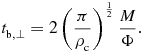 $$\begin{eqnarray}
t_{\rm b,\perp }=2 \left( \frac{\pi }{\rho _{\rm c}} \right)^\frac{1}{2}\frac{M}{\Phi }.
\end{eqnarray}$$
$$\begin{eqnarray}
t_{\rm b,\perp }=2 \left( \frac{\pi }{\rho _{\rm c}} \right)^\frac{1}{2}\frac{M}{\Phi }.
\end{eqnarray}$$
In the derivation, it is assumed that Alfvén waves propagate isotropically on the equatorial plane, and, as a consequence, B(r)∝r − 1 because of ∇ · B = 0. The ratio of the magnetic braking timescale of parallel and perpendicular configurations from Equations (5) and (8) is given as
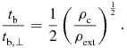 $$\begin{eqnarray}
\frac{t_{\rm b}}{t_{\rm b,\perp }}=\frac{1}{2}\left(\frac{\rho _{\rm c}}{\rho _{\rm ext}} \right)^{\frac{1}{2}}.
\end{eqnarray}$$
$$\begin{eqnarray}
\frac{t_{\rm b}}{t_{\rm b,\perp }}=\frac{1}{2}\left(\frac{\rho _{\rm c}}{\rho _{\rm ext}} \right)^{\frac{1}{2}}.
\end{eqnarray}$$
This shows that the timescale in perpendicular case is much smaller than that in the parallel case because ρc ≫ ρext, meaning that the magnetic braking in the perpendicular case is much stronger than that in the parallel case. However, in realistic case, fanned-out configuration of magnetic field should be considered as shown in Figure 4. Thus, the ratio of the timescale becomes
 $$\begin{eqnarray}
\frac{t_{\rm b,f}}{t_{\rm b,\perp }}=\frac{1}{2}\left(\frac{\rho _{\rm c}}{\rho _{\rm ext}} \right)^{\frac{1}{2}}\left(\frac{R_{\rm c}}{R_{\rm ext}}\right)^2.
\end{eqnarray}$$
$$\begin{eqnarray}
\frac{t_{\rm b,f}}{t_{\rm b,\perp }}=\frac{1}{2}\left(\frac{\rho _{\rm c}}{\rho _{\rm ext}} \right)^{\frac{1}{2}}\left(\frac{R_{\rm c}}{R_{\rm ext}}\right)^2.
\end{eqnarray}$$
This shows that magnetic braking timescale of the perpendicular case can be larger than that of the parallel case when
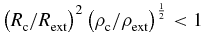 $\left(R_{\rm c}/R_{\rm ext}\right)^2 \left(\rho _{\rm c}/\rho _{\rm ext} \right)^{\frac{1}{2}} <1$
. However, whether the magnetic braking in the perpendicular case is weaker than that in the parallel case is not obvious because it is difficult to quantitatively compare (R
c/R
ext)2 and
$\left(R_{\rm c}/R_{\rm ext}\right)^2 \left(\rho _{\rm c}/\rho _{\rm ext} \right)^{\frac{1}{2}} <1$
. However, whether the magnetic braking in the perpendicular case is weaker than that in the parallel case is not obvious because it is difficult to quantitatively compare (R
c/R
ext)2 and
 $\left(\rho _{\rm c}/\rho _{\rm ext} \right)^{\frac{1}{2}}$
from the analytic discussions.
$\left(\rho _{\rm c}/\rho _{\rm ext} \right)^{\frac{1}{2}}$
from the analytic discussions.
Several multidimensional simulations have been performed to investigate the magnetic braking in the misaligned configuration, however, the results are inconsistent among the previous studies (Matsumoto & Tomisaka Reference Matsumoto and Tomisaka2004; Machida et al. Reference Machida, Matsumoto, Hanawa and Tomisaka2006; Hennebelle & Ciardi Reference Hennebelle and Ciardi2009; Joos et al. Reference Joos, Hennebelle and Ciardi2012; Li et al. Reference Li, Krasnopolsky and Shang2013). Matsumoto & Tomisaka (Reference Matsumoto and Tomisaka2004) conducted ideal MHD simulations of the collapsing cloud core using a Bonnor–Ebert sphere. They investigated the angular momentum evolution of the prestellar collapse phase and reported that the angular momentum of the central region is more efficiently removed when the magnetic field and rotation vector are perpendicular. This is consistent with the classical estimate of Mouschovias & Paleologou (Reference Mouschovias and Paleologou1979). In Figure 6, we show the angular momentum evolution of the central region obtained in Matsumoto & Tomisaka (Reference Matsumoto and Tomisaka2004). The figure shows that the angular momentum in the central region in the perpendicular case (SF90) is much smaller than that in the parallel case (SF00).
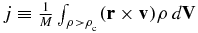
Evolution of central angular momentum as a function of maximum (or central) density ρmax. Here, J ≡ ∫ρ > 0.1ρmax (r × v)ρ d V and M ≡ ∫ρ > 0.1ρmax ρ d V. This figure appears as Figure 12 of Matsumoto & Tomisaka (Reference Matsumoto and Tomisaka2004). Models SF00, SF45, and SF90 denote the simulation results with a mutual angle between the initial magnetic field and the initial rotation vector of θ = 0°, 45°, and 90°. The dashed line denotes J/M 2 for an unmagnetised simulation. The solid lines denote the angular momentum parallel to the local magnetic field, J ∥/M 2, whereas dotted lines denote the angular momentum perpendicular to the local magnetic field, J ⊥/M 2. Dash–dotted line denotes J ∥ for a simulation with a weak magnetic field and dashed line denotes J for a simulation without magnetic field. Diamonds denote the stage of the first core formation epoch. Solid line of SF00 and dotted line of SF90 clearly show that the angular momentum around the central region with a perpendicular magnetic field is much smaller than that with a parallel magnetic field.

On the other hand, Hennebelle & Ciardi (Reference Hennebelle and Ciardi2009) reported that the efficiency of the magnetic braking decreases as the mutual angle between the magnetic field and the rotation axis increases and is minimum in the perpendicular configuration using centrally condensed cloud core with magnetic field whose intensity is proportional to the total column density through the core. They pointed out that disk formation becomes possible in the misaligned cloud cores even in the ideal MHD limit. Joos et al. (Reference Joos, Hennebelle and Ciardi2012) also conducted the ideal MHD simulations with the same density profile of Hennebelle & Ciardi (Reference Hennebelle and Ciardi2009). Figure 7 is taken from Figure 4 of Joos et al. (Reference Joos, Hennebelle and Ciardi2012) and shows that mean specific angular momentum of the central dense region in a perpendicular core (red lines) is about two times larger than that in a parallel core (blue lines). This is clearly opposite to the result shown in Figure 6. The influence of misalignment was also investigated by Li et al. (Reference Li, Krasnopolsky and Shang2013) with uniform density sphere. They also reported that the angular momentum of the central region is much large in the perpendicular case and concluded that the disk formation becomes possible when μ ≳ 4. They pointed out that the angular momentum removal by outflow plays an important role in the parallel configuration.
Evolution of mean specific angular momentum as a function of time. This figure appears as Figure 4 in Joos et al. (Reference Joos, Hennebelle and Ciardi2012). Here, the mean specific angular momentum is defined as
 $j \equiv \frac{1}{M} \int _{\rho >\rho _{\rm c}}(\boldsymbol{r \times v} )\rho \, d \boldsymbol{V}$
and M ≡ ∫ρ > ρc
ρ d
V. Evolution with μ = 5 and three different thresholds, ρc that correspond to n = 1010, 109, 108cm− 3 is shown.
$j \equiv \frac{1}{M} \int _{\rho >\rho _{\rm c}}(\boldsymbol{r \times v} )\rho \, d \boldsymbol{V}$
and M ≡ ∫ρ > ρc
ρ d
V. Evolution with μ = 5 and three different thresholds, ρc that correspond to n = 1010, 109, 108cm− 3 is shown.

It is still unclear why the discrepancy between the results of Hennebelle & Ciardi (Reference Hennebelle and Ciardi2009), Joos et al. (Reference Joos, Hennebelle and Ciardi2012), Li et al. (Reference Li, Krasnopolsky and Shang2013), and Matsumoto & Tomisaka (Reference Matsumoto and Tomisaka2004) arises. One possible explanation is the difference in the initial conditions. As discussed above, the magnetic braking timescale in the perpendicular configuration can be larger or smaller than that in the parallel configuration depending on the assumptions of the envelope structure and magnetic field configurations. Hence, the difference in the initial conditions may explain the discrepancy although further studies on the effect of misalignment on the magnetic braking efficiency are required.
6 INFLUENCE OF NON-IDEAL MHD EFFECTS ON DISK FORMATION
So far, we have reviewed the mechanisms that weaken magnetic braking in the ideal MHD limit. In a realistic molecular cloud core, however, the ideal MHD approximation, in which infinite conductivity is assumed, is not always valid because of the small ionisation degree. Thus, non-ideal effects may affect the formation and evolution of circumstellar disks. In this section, we review the influence of non-ideal MHD effects on disk formation.
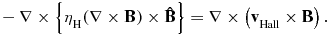
In a weakly ionised gas, collisions between neutral, positively charged, and negatively charged particles cause finite conductivity, and non-ideal effects arise. The non-ideal effects appear as correction terms in the induction equation if we neglect the inertia of the charged particles. The induction equation with non-ideal terms is given as
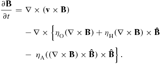 $$\begin{eqnarray}
\frac{\partial \boldsymbol{B}}{\partial t} &=& \nabla \times (\boldsymbol{v}\times \boldsymbol{B})\nonumber \\
&&-\, \nabla \times \left\lbrace \eta _{\rm O} (\nabla \times \boldsymbol{B}) +\eta _{\rm H} (\nabla \times \boldsymbol{B}) \times \boldsymbol{\hat{B}} \right.\nonumber\\
&&-\, \left. \eta _{\rm A} ((\nabla \times \boldsymbol{B}) \times \boldsymbol{\hat{B}}) \times \boldsymbol{\hat{B}}\right\rbrace .
\end{eqnarray}$$
$$\begin{eqnarray}
\frac{\partial \boldsymbol{B}}{\partial t} &=& \nabla \times (\boldsymbol{v}\times \boldsymbol{B})\nonumber \\
&&-\, \nabla \times \left\lbrace \eta _{\rm O} (\nabla \times \boldsymbol{B}) +\eta _{\rm H} (\nabla \times \boldsymbol{B}) \times \boldsymbol{\hat{B}} \right.\nonumber\\
&&-\, \left. \eta _{\rm A} ((\nabla \times \boldsymbol{B}) \times \boldsymbol{\hat{B}}) \times \boldsymbol{\hat{B}}\right\rbrace .
\end{eqnarray}$$
The second, third, and fourth terms on the right-hand side of Equation (11) describe Ohmic diffusion, the Hall term, and ambipolar diffusion, respectively. Here, ηO, ηH, and ηA are the Ohmic, Hall, and ambipolar diffusion coefficients, respectively. These quantities are calculated from the microscopic force balance of ions, electrons, and charged dust aggregates.
Detailed calculations of the abundance of charged particles are required to quantify how the non-ideal effects influence disk formation. For example, we show the evolution of the abundance of ions, electrons, and charged dusts inside the cloud core as a function of the density in Figure 8. This figure appears as Figure 1 of Nakano et al. (Reference Nakano, Nishi and Umebayashi2002). The figure shows that the relative abundance of the charged particles decreases as the density increases. The figure also shows that the dominant charge carriers are ions and electrons in the low density region n H ≲ 106cm− 3 and g+ and g− are the dominant carriers in the high density region 1010 < n Hcm− 3.
Abundances of various charged particles as a function of the density of hydrogen nuclei. This figure appears as Figure 1 of Nakano, Nishi, & Umebayashi (Reference Nakano, Nishi and Umebayashi2002). Here, n
H denotes the number density of hydrogen nuclei. Solid and dotted lines represent the number densities of ions, and electrons relative to n
H, respectively. Dashed lines labelled g
x
represent the number densities relative to n
H of grains of charge xe summed over the radius. The ionisation rate of a H2 molecule by cosmic rays outside the cloud core is taken to be
 $\zeta _0=10^{-17} \text{ s}^{-1}$
. M+ and m+ collectively denote metal ions such as Mg+, Si+, and Fe+ and molecular ions such as HCO+, respectively. The MRN dust size distribution (Mathis, Rumpl, & Nordsieck Reference Mathis, Rumpl and Nordsieck1977) with
$\zeta _0=10^{-17} \text{ s}^{-1}$
. M+ and m+ collectively denote metal ions such as Mg+, Si+, and Fe+ and molecular ions such as HCO+, respectively. The MRN dust size distribution (Mathis, Rumpl, & Nordsieck Reference Mathis, Rumpl and Nordsieck1977) with
 $a_{\rm min}=0.005\ \mu \text{m}$
and
$a_{\rm min}=0.005\ \mu \text{m}$
and
 $a_{\rm max}=0.25\ \mu \text{m}$
is assumed.
$a_{\rm max}=0.25\ \mu \text{m}$
is assumed.

6.1 Ohmic and ambipolar diffusion
6.1.1 Magnetic flux-loss in the first core phase
The effect of Ohmic and ambipolar diffusions in the collapsing cloud core has been thoroughly investigated by Nakano and his collaborators using an analytic approach (Nakano Reference Nakano1984; Nakano & Umebayashi Reference Nakano and Umebayashi1986; Umebayashi & Nakano Reference Umebayashi and Nakano1990; Nishi, Nakano, & Umebayashi Reference Nishi, Nakano and Umebayashi1991; Nakano et al. Reference Nakano, Nishi and Umebayashi2002). They investigated the influence of magnetic diffusion during cloud core collapse by comparing the diffusion timescale of magnetic field and the free-fall timescale.
Figure 9 shows the typical evolution of the magnetic diffusion timescale in the cloud core. The magnetic diffusion timescale becomes smaller than the free-fall timescale at a density of n crit ~ 1011cm− 3, and much of the magnetic flux is removed from the gas in the central region when the central density reaches n crit. They pointed out that this flux-loss is caused mainly by Ohmic diffusion. The critical density varies according to the dust model. Nishi et al. (Reference Nishi, Nakano and Umebayashi1991) investigated the dependence of the critical density on the dust model and found that the critical density varies in the range of 1010cm− 3 ≲ n crit ≲ 1011cm− 3.
Timescales of magnetic flux-loss for cloud cores. This figure appears as Figure 3 of Nakano et al. (Reference Nakano, Nishi and Umebayashi2002). The flux-loss timescale t
B is shown for field strengths of B = B
cr (solid lines) and B = 0.1B
cr (dashed lines), where B
cr approximately corresponds to the magnetic field strength of μ ~ 1 [the exact value of B
cr can be found in Equation (30) of Nakano et al. (Reference Nakano, Nishi and Umebayashi2002)]. The Ohmic diffusion time t
od is also shown as dash–dotted lines. Two ionisation rates by cosmic rays outside the cloud core,
 $\zeta _0=10^{-17}\, \text{s}^{-1}$
(thick lines: standard case) and
$\zeta _0=10^{-17}\, \text{s}^{-1}$
(thick lines: standard case) and
 $\zeta _0=10^{-16}\, \text{s}^{-1}$
(thin lines), are considered. The other parameters are the same as in Figure 8. Dotted line indicates the free-fall time t
ff = [3π/(32Gρ)]1/2.
$\zeta _0=10^{-16}\, \text{s}^{-1}$
(thin lines), are considered. The other parameters are the same as in Figure 8. Dotted line indicates the free-fall time t
ff = [3π/(32Gρ)]1/2.

As discussed in Section 3, the pressure-supported first core is formed when the central density reaches n ~ 1010cm− 3, and significant flux-loss occurs in the first core phase. Furthermore, the duration of the first core phase is much longer than the free-fall timescale and the magnetic flux-loss may occur at a density less than n crit. Thus, it is expected that the magnetic field and the gas are decoupled in the first core and that the magnetic braking is no longer important in it.
6.1.2 Formation of circumstellar disk in the first core phase
Multidimensional MHD simulations with magnetic diffusion have been conducted and have revealed its influence on early disk evolution (Duffin & Pudritz Reference Duffin and Pudritz2009; Machida & Matsumoto Reference Machida and Matsumoto2011; Li et al. Reference Li, Krasnopolsky and Shang2011; Tomida et al. Reference Tomida, Tomisaka, Matsumoto, Hori, Okuzumi, Machida and Saigo2013, Reference Tomida, Okuzumi and Machida2015; Tsukamoto et al. Reference Tsukamoto, Iwasaki, Okuzumi and Machida2015b; Masson et al. Reference Masson, Chabrier, Hennebelle, Vaytet and Commerçon2015). As we described above, the magnetic field and the gas is decoupled in the first core. Decoupling between the magnetic field and the gas in the first core leads to a very important consequence for disk formation because the first core is the precursor of the circumstellar disk. Machida & Matsumoto (Reference Machida and Matsumoto2011) conducted numerical simulations that followed formation of the protostar without any sink technique. They clearly showed that the first core directly becomes the circumstellar disk after the second collapse. In Figure 10, we show the structure of the forming circumstellar disk inside the first core at the protostar formation epoch. Because the first core has finite angular momentum and magnetic braking is no longer important in it, the gas cannot accrete directly onto the second core owing to centrifugal force. Therefore, the circumstellar disk inevitably forms just after protostar formation.
Remnant of the first core (orange isodensity surface) and forming circumstellar disk (red isodensity surface) plotted in three dimensions. This figure appears as Figure 3 of Machida & Matsumoto (Reference Machida and Matsumoto2011). Density distributions on the x = 0, y = 0, and z = 0 planes are projected onto each wall surface. Velocity vectors on the z = 0 plane are also projected onto the bottom wall surface.

The disk formation at the protostar formation epoch was later confirmed by more sophisticated simulations that included radiative transfer and Ohmic and ambipolar diffusion (Tomida et al. Reference Tomida, Tomisaka, Matsumoto, Hori, Okuzumi, Machida and Saigo2013, Reference Tomida, Okuzumi and Machida2015; Tsukamoto et al. Reference Tsukamoto, Iwasaki, Okuzumi and Machida2015b; Masson et al. Reference Masson, Chabrier, Hennebelle, Vaytet and Commerçon2015). All of them reported formation of a circumstellar disks at the protostar formation epoch due to magnetic diffusion, although slight differences exist in the initial size of the circumstellar disk (1AU ≲ r ≲ 10AU), which may arise from differences in the initial conditions, EOS, or resistivity models. Because the magnetic field and the gas are inevitably decoupled in the first core, we robustly conclude that the circumstellar disk with a size of r ≳ 1 AU is formed at the protostar formation epoch.
The circumstellar disk serves as a reservoir for angular momentum. As pointed out in the classical theory of an accretion disk (Lynden-Bell & Pringle Reference Lynden-Bell and Pringle1974), the gas accreted onto the disk leaves most of the angular momentum in the disk and accretes onto the protostar. Therefore, a small disk can grow in the subsequent evolution phase even though it is small at its formation epoch.
6.1.3 Properties and long term evolution of newborn disk
The newborn circumstellar disk is expected to be more massive than the newborn protostar at its formation epoch. This was clearly noted by Inutsuka et al. (Reference Inutsuka, Machida and Matsumoto2010). Figure 11 shows a schematic figure of the evolution of the characteristic mass scale during gravitational collapse and the accretion phase. The masses of the newborn protostar and the first core are roughly determined by the Jeans mass and are approximately 10− 3 and
 $10^{-2}\, \text{M}_\odot$
, respectively (Masunaga, Miyama, & Inutsuka Reference Masunaga, Miyama and Inutsuka1998; Masunaga & Inutsuka Reference Masunaga and Inutsuka1999). In addition, the newborn circumstellar disk acquires most of the mass of the first core. Thus, the circumstellar disk is more massive than the central protostar at its formation epoch. In such a massive disk, gravitational instability (GI) serves as an important angular momentum transfer mechanism. Later, Machida et al. (Reference Machida, Inutsuka and Matsumoto2011b), Tsukamoto et al. (Reference Tsukamoto, Iwasaki, Okuzumi and Machida2015b) confirmed that a newborn disk is actually massive, and GI may serve as the angular momentum transfer mechanism in the early phase of circumstellar disk evolution.
$10^{-2}\, \text{M}_\odot$
, respectively (Masunaga, Miyama, & Inutsuka Reference Masunaga, Miyama and Inutsuka1998; Masunaga & Inutsuka Reference Masunaga and Inutsuka1999). In addition, the newborn circumstellar disk acquires most of the mass of the first core. Thus, the circumstellar disk is more massive than the central protostar at its formation epoch. In such a massive disk, gravitational instability (GI) serves as an important angular momentum transfer mechanism. Later, Machida et al. (Reference Machida, Inutsuka and Matsumoto2011b), Tsukamoto et al. (Reference Tsukamoto, Iwasaki, Okuzumi and Machida2015b) confirmed that a newborn disk is actually massive, and GI may serve as the angular momentum transfer mechanism in the early phase of circumstellar disk evolution.
Schematic of evolution of the characteristic mass during gravitational collapse of the molecular cloud cores. This figure appears as Figure 2 of Inutsuka et al. (Reference Inutsuka, Machida and Matsumoto2010). The vertical axis denotes mass (in units of solar mass) and the horizontal axis denotes time (in years). The red curve on the left-hand side indicates the characteristic mass of the collapsing molecular cloud core, which corresponds to the Jeans mass. Note that the mass of the first core is much larger than that of the central protostar at its birth. The right-hand side describes the evolution after protostar formation. Because the first core changes into the circumstellar disk, the disk mass remains larger than the mass of the protostar in its early evolutionary phase. The protostar mass increases monotonically owing to mass accretion from the disk and becomes larger than the mass of the disk at some point.

The disk evolves by mass accretion from the envelope. How the disk size increases in the Class 0 phase depends strongly on the amount of angular momentum carried into the disk. Using long-term simulations with a sink cell, Machida et al. (Reference Machida, Inutsuka and Matsumoto2011b) showed that a disk can grow to the 100 AU scale when the envelope is depleted (i.e., at the end of the Class 0 phase). Note that magnetic braking becomes weak once the envelope is depleted because the magnetic braking timescale depends on the envelope density [see, Equations (5) and (7)].
6.2 Hall effect
The Hall effect has an unique feature in that it can actively induce rotation by generating a toroidal magnetic field from a poloidal magnetic field (Wardle & Ng Reference Wardle and Ng1999). In this subsection, we review the influence of the Hall effect on circumstellar disk formation and evolution.
For understanding how magnetic field evolves with the Hall effect, we rewrite the Hall term in the induction equation as
 $$\begin{eqnarray}
-\nabla \times \left\lbrace \eta _{\rm H} (\nabla \times \boldsymbol{B}) \times \boldsymbol{\hat{B}}\right\rbrace =\nabla \times \left( \boldsymbol{v}_{\rm Hall} \times \boldsymbol{B}\right) .
\end{eqnarray}$$
$$\begin{eqnarray}
-\nabla \times \left\lbrace \eta _{\rm H} (\nabla \times \boldsymbol{B}) \times \boldsymbol{\hat{B}}\right\rbrace =\nabla \times \left( \boldsymbol{v}_{\rm Hall} \times \boldsymbol{B}\right) .
\end{eqnarray}$$
Here, the drift velocity induced by the Hall term is defined as
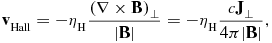 $$\begin{eqnarray}
\boldsymbol{v}_{\rm Hall}=-\eta _{\rm H} \frac{(\nabla \times \boldsymbol{B})_\perp }{|\boldsymbol{B}|}=-\eta _{\rm H}\frac{c \boldsymbol{J}_\perp }{4 \pi |\boldsymbol{B}|},
\end{eqnarray}$$
$$\begin{eqnarray}
\boldsymbol{v}_{\rm Hall}=-\eta _{\rm H} \frac{(\nabla \times \boldsymbol{B})_\perp }{|\boldsymbol{B}|}=-\eta _{\rm H}\frac{c \boldsymbol{J}_\perp }{4 \pi |\boldsymbol{B}|},
\end{eqnarray}$$
where c is the speed of light. The right-hand side of Equation (12) has the same form as the ideal MHD term. The Equations (12) and (13) show that the magnetic field moves along J ⊥ with a speed of |v Hall|.
During gravitational collapse, an hourglass-shaped magnetic field is generally realised (see Figure 3). In this configuration, a toroidal current exists at the midplane and the Hall term generates a toroidal magnetic field by twisting the magnetic field lines toward the azimuthal direction. The toroidal magnetic field exerts a toroidal magnetic tension and induces gas rotation. Consequently, the gas starts to rotate even when it does not rotate initially. This phenomenon was actually observed in the simulations of Krasnopolsky et al. (Reference Krasnopolsky, Li and Shang2011) and Li et al. (Reference Li, Krasnopolsky and Shang2011).
The characteristic rotation velocity induced by the Hall effect can be estimated from the Hall drift velocity v Hall because the toroidal component of the ideal term and the Hall term cancel each other out when the rotation velocity is equal to the azimuthal component of the Hall drift velocity v Hall, ϕ. Thus, the rotation velocity of the gas tends to converge to v ϕ = v Hall, ϕ. Using the numerical simulations in which only Hall effect is considered, Krasnopolsky et al. (Reference Krasnopolsky, Li and Shang2011) showed that the rotation velocity actually converges to v Hall, ϕ.
Here, we estimate the Hall-induced rotation velocity in the pseudodisk in which a current sheet exists at the midplane. The rotation velocity induced by the Hall term is roughly estimated as
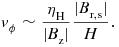 $$\begin{eqnarray}
v_{\rm \phi } \sim \frac{\eta _{\rm H}}{|B_{\rm z}|}\frac{|B_{\rm r,s}|}{H}.
\end{eqnarray}$$
$$\begin{eqnarray}
v_{\rm \phi } \sim \frac{\eta _{\rm H}}{|B_{\rm z}|}\frac{|B_{\rm r,s}|}{H}.
\end{eqnarray}$$
Here, H, B z, and B r, s are the scale height, vertical magnetic field at the midplane, and radial magnetic field at the surface of the pseudodisk, respectively, and we assumed |∇ × B| ~ |B r, s|/H. It is clear from the Equation (14) that, because ηH is proportional to |B|, the Hall-induced rotation velocity is an increasing function of the strength of the magnetic field. By employing the monopole approximation B r, s ~ Φpdisk/(2πr 2) which is used in Contopoulos, Ciolek, & Königl (Reference Contopoulos, Ciolek and Königl1998), Krasnopolsky & Königl (Reference Krasnopolsky and Königl2002), and Braiding & Wardle (Reference Braiding and Wardle2012b, Reference Braiding and Wardle2012a) and using the relation of Φpdisk = M pdisk/(μpdisk(M/Φ)crit), we can estimate the Hall-induced rotation velocity as
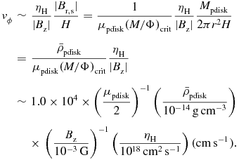 $$\begin{eqnarray}
v_{\rm \phi } &\sim& \frac{\eta _{\rm H}}{|B_{\rm z}|}\frac{|B_{\rm r,s}|}{H} = \frac{1}{\mu _{\rm pdisk} (M/\Phi )_{\rm crit}} \frac{\eta _{\rm H}}{|B_{\rm z}|}\frac{M_{\rm pdisk}}{2 \pi r^2 H}\nonumber\\
&=&\frac{\bar{\rho }_{\rm pdisk}}{\mu _{\rm pdisk} (M/\Phi )_{\rm crit}} \frac{\eta _{\rm H}}{|B_{\rm z}|} \nonumber\\
&\sim& 1.0 \times 10^{4} \times \left( \frac{\mu _{\rm pdisk}}{2}\right)^{-1} \left( \frac{\bar{\rho }_{\rm pdisk}}{10^{-14} \,{\rm g\,cm}^{-3} } \right)\nonumber \\
&&\times\, \left( \frac{B_{\rm z}}{10^{-3} \,{\rm G}} \right)^{-1} \left( \frac{\eta _{\rm H}}{ 10^{18} \,{\rm cm}^{2} \,{\rm s}^{-1} }\right) ({\rm cm\,s^{-1}}).
\end{eqnarray}$$
$$\begin{eqnarray}
v_{\rm \phi } &\sim& \frac{\eta _{\rm H}}{|B_{\rm z}|}\frac{|B_{\rm r,s}|}{H} = \frac{1}{\mu _{\rm pdisk} (M/\Phi )_{\rm crit}} \frac{\eta _{\rm H}}{|B_{\rm z}|}\frac{M_{\rm pdisk}}{2 \pi r^2 H}\nonumber\\
&=&\frac{\bar{\rho }_{\rm pdisk}}{\mu _{\rm pdisk} (M/\Phi )_{\rm crit}} \frac{\eta _{\rm H}}{|B_{\rm z}|} \nonumber\\
&\sim& 1.0 \times 10^{4} \times \left( \frac{\mu _{\rm pdisk}}{2}\right)^{-1} \left( \frac{\bar{\rho }_{\rm pdisk}}{10^{-14} \,{\rm g\,cm}^{-3} } \right)\nonumber \\
&&\times\, \left( \frac{B_{\rm z}}{10^{-3} \,{\rm G}} \right)^{-1} \left( \frac{\eta _{\rm H}}{ 10^{18} \,{\rm cm}^{2} \,{\rm s}^{-1} }\right) ({\rm cm\,s^{-1}}).
\end{eqnarray}$$
Here, Φpdisk, μpdisk, M
pdisk, and
 $ \bar{\rho }_{\rm pdisk}$
are the magnetic flux, the mass-to-flux ratio normalised by the critical value, the mass, and the mean density of the pseudodisk, respectively. Note that B
z is the vertical magnetic field at a radius, on the other hand, B
r, s is determined by the magnetic flux within a radius. Therefore, we need two different pieces of information (μpdisk and B
z) for magnetic field. Note also that Φpdisk (and hence B
r, s) increases as the total mass in the central region is increased by mass accretion if there is no efficient magnetic flux loss mechanism. Hence, the Hall-induced rotation would be strengthened in the later evolution phase. The corresponding specific angular momentum induced by the Hall term is estimated as
$ \bar{\rho }_{\rm pdisk}$
are the magnetic flux, the mass-to-flux ratio normalised by the critical value, the mass, and the mean density of the pseudodisk, respectively. Note that B
z is the vertical magnetic field at a radius, on the other hand, B
r, s is determined by the magnetic flux within a radius. Therefore, we need two different pieces of information (μpdisk and B
z) for magnetic field. Note also that Φpdisk (and hence B
r, s) increases as the total mass in the central region is increased by mass accretion if there is no efficient magnetic flux loss mechanism. Hence, the Hall-induced rotation would be strengthened in the later evolution phase. The corresponding specific angular momentum induced by the Hall term is estimated as
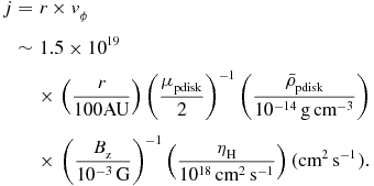 $$\begin{eqnarray}
j&=&r\times v_{\rm \phi }\nonumber \\
&\sim& 1.5 \times 10^{19} \nonumber\\
&& \times\,\left( \frac{r}{100 {\rm AU}} \right) \left( \frac{\mu _{\rm pdisk}}{2}\right)^{-1} \left( \frac{\bar{\rho }_{\rm pdisk}}{10^{-14} \,{\rm g\,cm}^{-3} } \right) \nonumber\\
&& \times\,\left( \frac{B_{\rm z}}{10^{-3} \,{\rm G}} \right)^{-1} \left( \frac{\eta _{\rm H}}{ 10^{18} \,{\rm cm}^{2} \,{\rm s}^{-1} }\right) ({\rm cm^2\,s^{-1}}).
\end{eqnarray}$$
$$\begin{eqnarray}
j&=&r\times v_{\rm \phi }\nonumber \\
&\sim& 1.5 \times 10^{19} \nonumber\\
&& \times\,\left( \frac{r}{100 {\rm AU}} \right) \left( \frac{\mu _{\rm pdisk}}{2}\right)^{-1} \left( \frac{\bar{\rho }_{\rm pdisk}}{10^{-14} \,{\rm g\,cm}^{-3} } \right) \nonumber\\
&& \times\,\left( \frac{B_{\rm z}}{10^{-3} \,{\rm G}} \right)^{-1} \left( \frac{\eta _{\rm H}}{ 10^{18} \,{\rm cm}^{2} \,{\rm s}^{-1} }\right) ({\rm cm^2\,s^{-1}}).
\end{eqnarray}$$
Once a circumstellar disk is formed, the accreting gas leaves the most of the angular momentum in the disk and finally accretes onto the central protostar. Thus, during protostar formation, the disk acquires an angular momentum of
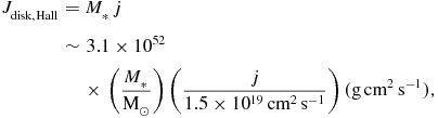 $$\begin{eqnarray}
J_{\rm disk, Hall}&=&M_*\,j \nonumber\\
&\sim& 3.1\times 10^{52} \nonumber\\
&&\times\,\left( \frac{M_*}{\text{M}_\odot } \right)\left( \frac{j}{1.5 \times 10^{19} \,{\rm cm^2\,s^{-1}}} \right) ({\rm g\,cm^2\,s^{-1}}),
\end{eqnarray}$$
$$\begin{eqnarray}
J_{\rm disk, Hall}&=&M_*\,j \nonumber\\
&\sim& 3.1\times 10^{52} \nonumber\\
&&\times\,\left( \frac{M_*}{\text{M}_\odot } \right)\left( \frac{j}{1.5 \times 10^{19} \,{\rm cm^2\,s^{-1}}} \right) ({\rm g\,cm^2\,s^{-1}}),
\end{eqnarray}$$
where M * is the final mass of the central protostar.
On the other hand, the total angular momentum of a Keplerian disk with Σ∝r − 3/2 is given as
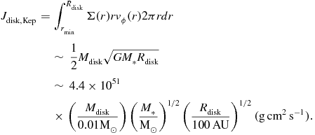 $$\begin{eqnarray}
J_{\rm disk, Kep}&=&\int _{r_{\rm min}}^{R_{\rm disk}} \Sigma (r) r v_{\phi }(r) 2 \pi r dr \nonumber\\
&&\sim \,\frac{1}{2} M_{\rm disk}\sqrt{G M_* R_{\rm disk}} \nonumber\\
&&\sim\, 4.4 \times 10^{51} \nonumber\\
&&\times\,\left( \frac{M_{\rm disk}}{0.01 \text{M}_\odot } \right) \left( \frac{M_*}{ \text{M}_\odot } \right)^{1/2}\left( \frac{R_{\rm disk}}{100 \,{\rm AU}} \right)^{1/2} ({\rm g\,cm^2\,s^{-1}}). \nonumber\\
\end{eqnarray}$$
$$\begin{eqnarray}
J_{\rm disk, Kep}&=&\int _{r_{\rm min}}^{R_{\rm disk}} \Sigma (r) r v_{\phi }(r) 2 \pi r dr \nonumber\\
&&\sim \,\frac{1}{2} M_{\rm disk}\sqrt{G M_* R_{\rm disk}} \nonumber\\
&&\sim\, 4.4 \times 10^{51} \nonumber\\
&&\times\,\left( \frac{M_{\rm disk}}{0.01 \text{M}_\odot } \right) \left( \frac{M_*}{ \text{M}_\odot } \right)^{1/2}\left( \frac{R_{\rm disk}}{100 \,{\rm AU}} \right)^{1/2} ({\rm g\,cm^2\,s^{-1}}). \nonumber\\
\end{eqnarray}$$
Thus, the Hall term alone can supply a sufficient amount of the angular momentum for explaining a circumstellar disk with a mass and radius of
 $0.01 \text{M}_\odot$
and 100 AU, respectively, which roughly correspond to typical values of the disks around T Tauri stars (Andrews & Williams Reference Andrews and Williams2005, Reference Andrews and Williams2007; Williams & Cieza Reference Williams and Cieza2011) .
$0.01 \text{M}_\odot$
and 100 AU, respectively, which roughly correspond to typical values of the disks around T Tauri stars (Andrews & Williams Reference Andrews and Williams2005, Reference Andrews and Williams2007; Williams & Cieza Reference Williams and Cieza2011) .
In realistic situations, the inherent rotation of cloud cores and magnetic diffusion introduce complicated gas dynamics. When the rotation of the cloud core is also considered, a very interesting phenomenon arises. As we can see from the induction equation, the Hall term is not invariant against inversion of the magnetic field (B → −B) and its effect on the gas rotation differs depending on whether the rotation vector and magnetic field of the host cloud core are parallel or antiparallel (Wardle & Ng Reference Wardle and Ng1999; Braiding & Wardle Reference Braiding and Wardle2012a, b). For ηH < 0 which is almost always valid in the cloud cores, when the rotation vector and magnetic field are antiparallel, the Hall-induced rotation and the inherent rotation are in the same direction, and hence, the Hall term weakens the magnetic braking. On the other hand, the Hall term strengthens the magnetic braking in the parallel case because the Hall term induces inverse rotation against the inherent rotation of the cloud core.
Krasnopolsky et al. (Reference Krasnopolsky, Li and Shang2011) investigated the effect of the Hall term on disk formation using two-dimensional simulations. They focused on the dynamical behaviour induced by the Hall term by neglecting Ohmic and ambipolar diffusion and by employing a constant Hall coefficient, Q Hall ≡ ηH|B|. They showed that a circumstellar disk r ≳ 10 AU in size can form as a result of only the Hall term when the Hall coefficient is Q Hall ≳ 3 × 1020cm2s− 1G− 1. Another interesting finding is that the formation of an envelope that rotates in the direction opposite to that of disk rotation. Because of the conservation of the angular momentum, the spin-up due to the Hall term at the midplane of the pseudodisk generates a negative angular momentum flux along the magnetic field line. This causes spin-down of the upper region, and the upper region eventually begins to rotate in the direction opposite to that of disk rotation.
Li et al. (Reference Li, Krasnopolsky and Shang2011) investigated the effect of the Hall term in two-dimensional simulations that included all the non-ideal MHD effects using a realistic diffusion model and started from uniform cloud cores. They confirmed that Hall-induced rotation occurs even when other non-ideal effects are considered. They also showed that the formation of a counter-rotating envelope. They showed that the Hall-induced rotation velocity can reach v ϕ ~ 105(cms− 1) at r = 1014(cm) (this corresponds to the radius of the their inner boundary), which means that the accreting gas has a specific angular momentum of j ~ 1019(cm2s− 1) (Figure 11 of Li et al. Reference Li, Krasnopolsky and Shang2011). This is consistent with the value estimated using Equation (16).
Tsukamoto et al. (Reference Tsukamoto, Iwasaki, Okuzumi and Machida2015a) conducted three-dimensional simulations, that included all the non-ideal effects as well as radiative transfer. They followed the first core formation phase and resolved protostar formation without any sink technique. Therefore, their simulations did not suffer from numerical artefacts introduced by the sink or inner boundary. A drawback of this treatment is that they could not follow the long-term evolution of the disk after protostar formation because the numerical timestep became very small. In Figure 12, we show a density map of the central regions of the simulations conducted in Tsukamoto et al. (Reference Tsukamoto, Iwasaki, Okuzumi and Machida2015a). The left panel shows the result of the simulation in which initial magnetic field and the rotation vector are in parallel configuration. On the other hand, the right panel shows that in which initial magnetic field and the rotation vector are in antiparallel configuration. The right panel clearly shows that a disk ~ 20 AU in size formed at the protostar formation epoch On the other hand, the left panel shows that a disk 1 AU in size formed even with the parallel configuration. They also showed that the magnetic field and the gas are decoupled in the disk in the right panel, and that the magnetic braking is no longer important in it. Although the disk is formed in both cases, the difference in its size in the parallel and antiparallel cases is significant. Thus, they argued that the disks in Class 0 YSOs can be subcategorised according to the parallel and antiparallel nature of their host cloud cores and suggested that the systems with parallel and antiparallel configurations should be called as ortho-disks and para-disks, respectively. They also confirmed that a negatively rotating envelope is formed and suggested that this envelope may be observable in future observations of Class 0 YSOs.
Density map of newborn disks formed in a cloud core with parallel configuration (left, model Ortho) and antiparallel configuration (right, model Para). This figure is taken from Figure 1 of Tsukamoto et al. (Reference Tsukamoto, Iwasaki, Okuzumi and Machida2015a) but it has been modified to clarify the formation of the disk in the model Ortho. In the simulations, all the non-ideal effects are considered. The only difference between the initial conditions of the models Ortho and Para is the direction of the magnetic field. Inset at upper left in the left-hand panel shows an enlarged density map around the centre of the model Ortho. It shows that a disk ~ 1 AU in size is formed at the centre in the parallel case. The right panel shows that a disk ~ 20 AU in size is formed at the centre in the antiparallel case. We confirmed that both disks are rotationally supported. The non-axisymmetric spiral arms in the right panel are created by gravitational instability. We confirmed that Toomre’s Q value was Q ~ 1.

Up to the present, Wurster, Price, & Bate (Reference Wurster, Price and Bate2015) have made the most comprehensive study regarding the impact of non-ideal MHD effects on disk evolution. They investigated the influences of each non-ideal MHD effect both independently and together using three-dimensional simulations. They pointed out that, among the three non-ideal effects, the Hall effect is the most important process for disk size. This suggests that including the Hall effect is crucial for investigating the formation and evolution process of circumstellar disks in magnetised cloud cores. They pointed out that an anticorrelation between the size and speed of the outflow and the size of the disk. This suggests that angular momentum transfer by the outflow is also important. In their simulations, a negatively rotating envelope is also formed. Note that the negatively rotating envelopes are formed in all multidimensional simulations with the Hall effect (Krasnopolsky et al. Reference Krasnopolsky, Li and Shang2011; Li et al. Reference Li, Krasnopolsky and Shang2011; Tsukamoto et al. Reference Tsukamoto, Iwasaki, Okuzumi and Machida2015a; Wurster et al. Reference Wurster, Price and Bate2015) and its formation seems to be robust. Therefore, the detection of a negatively rotating envelope would provide clear evidence that the Hall effect actually influences the angular momentum evolution.
7 SUMMARY AND FUTURE PERSPECTIVES
7.1. Summary
In this paper, we reviewed the formation and evolution processes of circumstellar disks in magnetised cloud cores, focusing in particular on the influence of magnetic braking. In the ideal MHD approximation and with an aligned magnetic field, magnetic braking is very efficient and, circumstellar disk formation is almost completely suppressed in a moderately magnetised cloud core (its mass-to-flux ratio is μ ~ 2) (Allen et al. Reference Allen, Li and Shu2003; Hennebelle & Fromang Reference Hennebelle and Fromang2008; Mellon & Li Reference Mellon and Li2008). This introduced a serious discrepancy between the observations and theory and was considered a very serious problem for disk formation theory.
However, various physical mechanisms have been proposed to solve the problem of catastrophic magnetic braking. For example, the misalignment between the magnetic field and the rotation axis (Hennebelle & Ciardi Reference Hennebelle and Ciardi2009; Joos et al. Reference Joos, Hennebelle and Ciardi2012) or turbulence (Santos-Lima et al. Reference Santos-Lima, de Gouveia Dal Pino and Lazarian2012; Seifried et al. Reference Seifried, Banerjee, Pudritz and Klessen2013) in the cloud core may weaken magnetic braking. Ohmic and ambipolar diffusions remove much of the magnetic flux in the first core and make it possible for circumstellar disks a few AU in size to form at the formation epoch of the protostar (Machida & Matsumoto Reference Machida and Matsumoto2011; Tomida et al. Reference Tomida, Tomisaka, Matsumoto, Hori, Okuzumi, Machida and Saigo2013, Reference Tomida, Okuzumi and Machida2015; Tsukamoto et al. Reference Tsukamoto, Takahashi, Machida and Inutsuka2015c; Masson et al. Reference Masson, Chabrier, Hennebelle, Vaytet and Commerçon2015). The spin-up effect of the Hall term increases the specific angular momentum of the accretion flow and the disk radius at the protostar formation epoch (Krasnopolsky et al. Reference Krasnopolsky, Li and Shang2011; Tsukamoto et al. Reference Tsukamoto, Iwasaki, Okuzumi and Machida2015a). A combination of these mechanisms solves the magnetic braking problem, and we can robustly conclude that the disk is formed in the early evolution phase of the protostar, although its quantitative features, such as the disk radius and mass, are still under debate. Therefore, the simple question of whether a disk can form is no longer a central issue, and we should move on to more specific problems of disk evolution.
7.2. Future perspectives
Determining the angular momentum transfer mechanisms in the Class 0 phase may be the most important unresolved issue. To data, GI and magneto-rotational instability (MRI) are considered to be the two major mechanisms of angular momentum transport within the disk (Armitage Reference Armitage2011). Further, magneto-centrifugal wind (Blandford & Payne Reference Blandford and Payne1982) has recently received attention as a mechanism that can remove angular momentum from a disk (Tomisaka Reference Tomisaka2000, Reference Tomisaka2002; Bai & Stone Reference Bai and Stone2013; Bai Reference Bai2013; Gressel et al. Reference Gressel, Turner, Nelson and McNally2015). How these mechanisms contribute to disk evolution and how the relative importance of GI, MRI, and magneto-centrifugal wind changes during disk evolution are still unclear. Surface density and temperature determine whether the disk is stable against GI and the size of the MRI dead zone. Magnetic field strength is closely related to the saturation level of MRI (Sano et al. Reference Sano, Inutsuka, Turner and Stone2004; Suzuki, Muto, & Inutsuka Reference Suzuki, Muto and Inutsuka2010) and strength of magneto-centrifugal wind. Thus, to answer the question, we must quantitatively investigate the long-term evolution of the surface density, temperature, and magnetic field of disk by considering all the relevant physical mechanisms.
The formation process of binaries or multiples in the Class 0 phase and its relation to disk evolution is another important issue. Fragmentation of the disk or the first core is considered a promising mechanism for binary formation (Matsumoto & Hanawa Reference Matsumoto and Hanawa2003; Machida et al. Reference Machida, Matsumoto, Hanawa and Tomisaka2005, Reference Machida, Tomisaka, Matsumoto and Inutsuka2008; Kratter et al. Reference Kratter, Matzner, Krumholz and Klein2010; Tsukamoto & Machida Reference Tsukamoto and Machida2013; Tsukamoto et al. Reference Tsukamoto, Takahashi, Machida and Inutsuka2015c). However, for realistic values of the magnetic field and rotation velocity (μ ~ 1 and βrot ~ 0.01, respectively), the fragmentation in the early phase of the protostar formation seems to be strongly suppressed. In particular, the formation of a binary with a separation of several tens of AU would be very difficult for realistic values (see, Figure 12 of Machida et al. Reference Machida, Tomisaka, Matsumoto and Inutsuka2008). On the other hand, the binary or multiple fraction of solar-type stars is about 0.6, which is quite high (Duquennoy & Mayor Reference Duquennoy and Mayor1991). Furthermore, the median orbital period of binaries is 190 yrs indicating that the typical separation is several tens of AU. This introduces a discrepancy between the observations and theoretical studies, that should be resolved in future studies. To determine whether fragmentation of the first core or the disk is the dominant formation mechanism of multiples, we should investigate how often the fragmentation of the disk and the first core can occur in cloud cores and whether the frequency of fragmentation is sufficient to explain the number of binaries or multiples fraction.
Dust coagulation in the disk and its impact on disk evolution is also an important issue. It is expected that dust coagulation occurs and that the size distribution of the dust particles in the disk changes (Dullemond & Dominik Reference Dullemond and Dominik2005; Okuzumi Reference Okuzumi2009). Once dust coagulation occurs and the dust size distribution changes during disk evolution, the magnetic resistivity is affected, and the gas dynamics can also be altered owing to this. Then, the dust coagulation process may be modified by the gas dynamics. Therefore, it is possible that the large-scale disk and the small scale dust distribution co-evolve. Such a co-evolution process of dust and the disk would be important not only for the evolution of YSOs but also for formation process of planetesimals.
ACKNOWLEDGEMENTS
I would like to thank M. N. Machida, T. Matsumoto, S. Okuzumi, S. Inutsuka, K. Iwasaki, D. Price, B. Commerçon, P. Hennebelle, and J. Wurster for fruitful discussions. I also thank the anonymous referee for his/her insightful comments.


