





1. Introduction
1.1. Algebraic Chow groups
A lot of information about the topology of a manifold can be understood via its homology. Similarly, in algebraic geometry, one can try to understand a variety by studying its subvarieties modulo some equivalence relation. One of the most common equivalence relations is rational equivalence:  $k$-dimensional subvarieties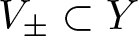 $V_\pm \subset Y$ of an algebraic variety $Y$ are said to be rationally equivalent if there exists a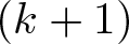 $(k+1)$-dimensional subvariety $W \subset Y \times \mathbb{P}^{1}$ whose projection to $\mathbb{P}^{1}$ is dominant and such that
 \begin{equation*}
V_\pm = W \cap (Y \times \left\lbrace{\pm\infty}\right\rbrace).
\end{equation*}
\begin{equation*}
V_\pm = W \cap (Y \times \left\lbrace{\pm\infty}\right\rbrace).
\end{equation*}where we denote by 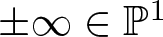 $\pm\infty\in\mathbb{P}^1$ the north and south pole of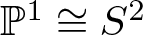 $\mathbb{P}^1\cong S^2$ (any two points of $\mathbb{P}^1$ could be used, however).
One defines the Chow groups of  $Y$ as the quotient
 \begin{equation}
\operatorname{CH}_k(Y) := Z_k(X)/R_k(X)
\end{equation}
\begin{equation}
\operatorname{CH}_k(Y) := Z_k(X)/R_k(X)
\end{equation}where 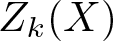 $Z_k(X)$ is the free abelian group generated by the $k$-dimensional subvarieties of $Y$ and $R_k(X) \subset Z_k(X)$ is the subgroup generated by differences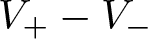 $V_+ - V_-$ for all rationally equivalent pairs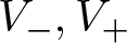 $V_-,V_+$.
Chow groups are classical objects in algebraic geometry and have been extensively studied. They are the subject of the Hodge conjecture and a series of conjectures due to Bloch and Beilinson. When  $Y$ is a curve, the Abel–Jacobi theorem—recall it identifies the Jacobian of a curve with its Albanese variety—proves these groups are isomorphic to $H_{2*}(Y) \oplus Jac(Y)$. However, as soon as we increase the dimension, these groups become notoriously difficult to compute. One of the first results along these lines is a classical theorem of Mumford in the 1960s [Reference Mumford15]. Mumford showed that when a smooth complex projective surface $Y$ admits a non-zero $2$-form—that is, when $0 \lt \dim H^{0}(\mathcal K_{Y})$, where $\mathcal K_Y$ is the canonical bundle of $Y$—the Chow group of points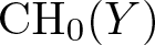 $\operatorname{CH}_0(Y)$ is infinite-dimensional in the following sense:
Definition 1.1 ([Reference Mumford15])
Let  $\operatorname{CH}_0(Y)_{\hom} \subset \operatorname{CH}_0(Y)$ be the subgroup of cycles of degree zero (that is, those linear combinations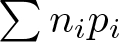 $\sum n_i p_i$ with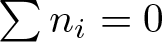 $\sum n_i = 0$). We write $\mathbf{y} = (y_1,\dots, y_k) \in Y^{k}$ to denote points in the $k$-th product of $Y$ with itself. We say $\operatorname{CH}_0(Y)_{\hom}$ is infinite-dimensional if the maps
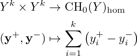 \begin{align*}
Y^k \times Y^k &\to \operatorname{CH}_0(Y)_{\hom}\\
(\mathbf{y}^+,\mathbf{y}^-)& \mapsto \sum_{i = 1}^k\left(y_i^+ - y_i^-\right)
\end{align*}
\begin{align*}
Y^k \times Y^k &\to \operatorname{CH}_0(Y)_{\hom}\\
(\mathbf{y}^+,\mathbf{y}^-)& \mapsto \sum_{i = 1}^k\left(y_i^+ - y_i^-\right)
\end{align*}are not surjective for any  $k$.
$k$.
Mumford’s result was later generalized by Roitman to higher dimensions [Reference Roitman16], showing that for any smooth projective algebraic variety  $Y$ over an uncountable field of characteristic zero, the existence of a non-zero $p$-form for some $p\geq2$ is enough to guarantee infinite-dimensionality of $\operatorname{CH}_0(Y)_{\hom}$.
The converse result—that is, whether the vanishing 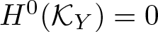 $H^0(\mathcal K_Y) = 0$ implies that $\operatorname{CH}_0(Y)_{\hom}$ is finite-dimensional—has been conjectured by Bloch [Reference Bloch4], and Bloch–Kas–Lieberman [Reference Bloch, Kas and Lieberman5] showed that this is true for surfaces with Kodaira dimension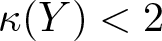 $\kappa(Y) \lt 2$.
1.2. Tropical Chow groups
An analogous equivalence relation for tropical geometry has appeared in the literature before, see e.g. [Reference Allermann, Hampe and Rau1, Definition 3.1]. Let us recall the equivalence relation therein (with a slight change of notation and nomenclature for convenience). In the following definition, given a tropical cycle  $C$ and a rational function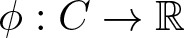 $\phi: C \to \mathbb{R}$, we denote by $\phi \cdot C$ the divisor of $\phi$. (A rational function on a tropical cycle is, roughly speaking, a piecewise-linear function with integer slope. Its divisor $\phi \cdot C$ is the locus where $\phi$ changes slope. We refer to the same paper [Reference Allermann, Hampe and Rau1] for precise definitions.)
Definition 1.2 ([Reference Allermann, Hampe and Rau1])
Let  $B$ be a tropical cycle and consider a $k$-dimensional subcycle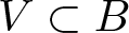 $V \subset B$. We say that $V$ is (bounded) rationally equivalent to zero on $B$ if there exists a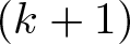 $(k+1)$-dimensional tropical cycle $f:C^{k+1} \to B$ and a (bounded) rational function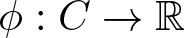 $\phi : C \to \mathbb{R}$ such that
 \begin{equation*}
V = f_*(\phi \cdot C).
\end{equation*}
\begin{equation*}
V = f_*(\phi \cdot C).
\end{equation*} We say that 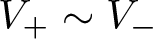 $V_+ \sim V_-$ are rationally equivalent if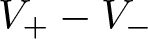 $V_+ - V_-$ is rationally equivalent to zero.
The setting in this paper is much more restrictive. We limit our attention and results to a subclass of tropical cycles  $B$ called tropical affine manifolds: these are smooth manifolds together with an integrable lattice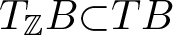 $T_{\mathbb{Z}} B {\subset} TB$ of tangent vectors. (An equivalent definition is a smooth manifold together with an atlas of charts whose transition functions belong to the group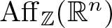 $\operatorname{Aff}_{\mathbb{Z}}(\mathbb{R}^n)$ of integral affine transformations of $\mathbb{R}^n$, i.e. those of the form $\mathbf{x} \mapsto A\mathbf{x} + \mathbf{x}_0, A \in \operatorname{GL}(n,\mathbb{Z})$.) Using Definition 1.2, one can define the tropical Chow groups just as in Equation (1), except now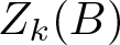 $Z_k(B)$ is generated by $k$-dimensional tropical subvarieties of $B$ and $R_k(B) \subset Z_k(B)$ by those differences $V_+ - V_- \in Z_k(B)$ such that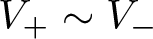 $V_+ \sim V_-$. Since we will only be working with the tropical Chow group of points (that is, the case $k = 0$), it is sufficient to say that a $1$-dimensional tropical subvariety—also known as a tropical curve—is a weighted, balanced rational polyhedral complex of pure dimension one [Reference Mikhalkin11] (see Figure 1(a)).
Examples of tropical curves. (a) Tropical curve inside  $\mathbb{R}^2$. The numbers next to the edges indicate the weight of each edge. At each vertex, the weighted sum of the outpointing primitive vectors vanishes. (b) Tropical curve in $B \times \mathbb{R}$ which is ‘horizontal at infinity’. It gives the relation $p_1^+ + p_2^+ = p_1^- + p_2^-$ in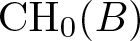 $\operatorname{CH}_0(B)$. As drawn, it could give a relation for both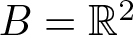 $B = \mathbb{R}^2$ and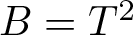 $B = T^2$.
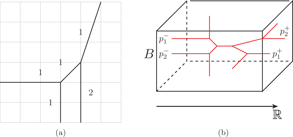
Figure 1 Long description
The image A shows a tropical curve within a grid. The curve consists of several edges, each labeled with a number indicating its weight. The curve starts at the bottom left, with an edge labeled '1' extending horizontally to the right. From this point, another edge labeled '1' extends vertically upwards. At the junction where these two edges meet, a third edge labeled '1' extends diagonally upwards to the right. Another edge labeled '1' extends vertically downwards from the junction. Finally, an edge labeled '2' extends vertically upwards from the bottom right corner of the grid. The image B shows a three-dimensional schematic labeled 'B' times 'R'. The diagram features several red lines within a box, representing relations. The box is drawn with solid and dashed lines to indicate its three-dimensional structure. Inside the box, red lines branch out from a central point, with labels 'p subscript 1 superscript minus', 'p subscript 2 superscript minus' and 'p subscript 1 superscript plus' positioned next to the respective lines. The box is oriented with an arrow pointing to the right, labeled 'R', indicating direction.
We show in Lemma 2.18 that the equivalence relation of Definition 1.2 is equivalent to the existence of a tropical curve in  $B \times \mathbb{R}$ that is ‘horizontal at infinity’ and asymptotic to $V_{\pm}$ at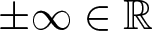 $\pm \infty \in \mathbb{R}$ (see Definition 2.16 for a precise definition and Figure 1(b) for a geometric intuition). The $0$-th tropical Chow group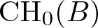 $\operatorname{CH}_0(B)$ is then the free abelian group on points of $B$ modulo relations induced by tropical curves in $B\times\mathbb{R}$ that are horizontal at infinity, as depicted in Figure 1(b).
Remark 1.3. Although we restrict the ambient space to be a tropical affine manifold (instead of an arbitrary tropical cycle like in [Reference Allermann, Hampe and Rau1]), note that the generators of 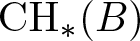 $\operatorname{CH}_*(B)$ are in fact arbitrary tropical cycles in $B$ (not only integral affine submanifolds of $B$).
$B$).
1.3. Main results
Let  $T_{\mathbb{Z}}^{*B}$ be the local system of abelian groups whose sections over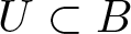 $U \subset B$ are differential $1$-forms $\alpha \in H^{0}(T^{*U})$ such that
 \begin{equation*}
\alpha(v)\in \mathbb{Z},\quad v \in T_{\mathbb{Z}} U.
\end{equation*}
\begin{equation*}
\alpha(v)\in \mathbb{Z},\quad v \in T_{\mathbb{Z}} U.
\end{equation*} Note that such sections are locally constant in affine coordinates. Let 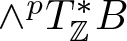 $\wedge^{p} T^{*}_{\mathbb{Z}} B$ be the exterior power of $T^{*}_{\mathbb{Z}} B$; global sections $\omega \in H^{0}(\wedge^{p} T^{*}_{\mathbb{Z}} B)$ are called tropical $p$-forms. The following is the main result of this paper:
Theorem A (= Theorem 3.7)
If a compact integral affine manifold  $B$ admits a non-zero tropical $p$-form for some $p \geq 2$, the group $\operatorname{CH}_0(B)_{\hom}$ is infinite dimensional (in the sense of Definition 1.1).
Note that, according to Theorem A, the existence of a non-zero tropical  $1$-form does not imply the tropical Chow group is infinite-dimensional. This can already be seen in the $1$-dimensional case: the tropical Abel–Jacobi theorem [Reference Mikhalkin and Zharkov13, Theorem 6.2] implies that a tropical circle has
 \begin{equation*}
\operatorname{CH}_{*}(S^{1}) \cong H_{*}(S^{1}) \oplus \operatorname{Jac}(S^{1}),
\end{equation*}
\begin{equation*}
\operatorname{CH}_{*}(S^{1}) \cong H_{*}(S^{1}) \oplus \operatorname{Jac}(S^{1}),
\end{equation*}which is finite-dimensional. Our second main result, Proposition B, shows that  $H^0(T_{\mathbb{Z}}^{*B}) \neq 0$ is also not sufficient to guarantee infinite-dimensionality of $\operatorname{CH}_0(B)_{\hom}$ even when $\dim B \gt 1$.
Let us first recall the definition of the tropical Albanese variety, which will replace the role of 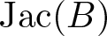 $\operatorname{Jac}(B)$ in the tropical Abel–Jacobi theorem. It is defined as the quotient
 \begin{equation*}
\operatorname{Alb}(B) = \frac{\operatorname{Hom}(H^0(T_{\mathbb{Z}}^*B),\mathbb{R})}{H_1(B;\mathbb{Z})}
\end{equation*}
\begin{equation*}
\operatorname{Alb}(B) = \frac{\operatorname{Hom}(H^0(T_{\mathbb{Z}}^*B),\mathbb{R})}{H_1(B;\mathbb{Z})}
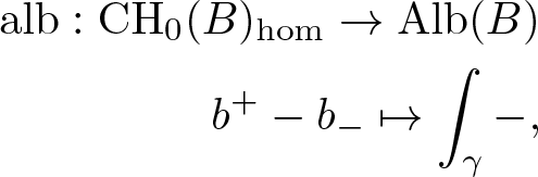
\end{equation*}where  $1$-cycles include into $\operatorname{Hom}(H^0(T_{\mathbb{Z}}^{*B}),\mathbb{R})$ via integration. The tropical Chow group of points of degree zero admits a map
 \begin{align*}
\operatorname{alb}:\operatorname{CH}_0(B)_{\hom} \to \operatorname{Alb}(B)\\
b^+-b_-\mapsto \int_\gamma -,
\end{align*}
\begin{align*}
\operatorname{alb}:\operatorname{CH}_0(B)_{\hom} \to \operatorname{Alb}(B)\\
b^+-b_-\mapsto \int_\gamma -,
\end{align*}where  $\gamma$ is any curve in $B$ with $\partial\gamma = b^+ - b^-$ (note that any two such $\gamma$ differ by a $1$-cycle, so the map is well-defined).
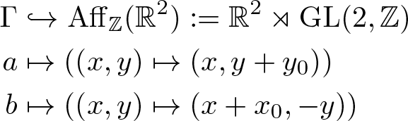
To show that the existence of tropical  $1$-forms is also not sufficient to guarantee infinite-dimensionality of $\operatorname{CH}_0(B)_{\hom}$ it is enough to consider the lowest dimensional case $\dim B = 2$. By dimension reasons $H^{0}(\wedge^{p} T_{\mathbb{Z}}^{*B}) = 0$ for $p \gt 2$, whereas $H^0(\wedge^{2} T_{\mathbb{Z}}^{*B}) = 0$ if and only if $B$ is non-orientable. The only $2$-dimensional closed integral affine manifolds (in particular, no singularities in the integral affine structure), which are non-orientable, are tropical Klein bottles. These have been classified by Sepe [Reference Sepe17]. We work with the following family of tropical Klein bottles (this is the family numbered by (3) in [Reference Sepe17] and called ‘Klein bottle of type I’ in [Reference Muñiz-Brea14]). Let $\Gamma = \langle a,b |aba = b \rangle$ be the fundamental group of a Klein bottle. We consider the injection
 \begin{equation}
\begin{split}
\Gamma &\hookrightarrow \operatorname{Aff}_{\mathbb{Z}} (\mathbb{R}^{2}) := \mathbb{R}^2 \rtimes \operatorname{GL}(2,\mathbb{Z})\\
a &\mapsto ((x,y)\mapsto (x, y + y_0))\\
b &\mapsto ((x,y)\mapsto (x + x_0, -y))
\end{split}
\end{equation}
\begin{equation}
\begin{split}
\Gamma &\hookrightarrow \operatorname{Aff}_{\mathbb{Z}} (\mathbb{R}^{2}) := \mathbb{R}^2 \rtimes \operatorname{GL}(2,\mathbb{Z})\\
a &\mapsto ((x,y)\mapsto (x, y + y_0))\\
b &\mapsto ((x,y)\mapsto (x + x_0, -y))
\end{split}
\end{equation}where 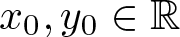 $x_0,y_0 \in \mathbb{R}$. The quotient
 \begin{equation*}
K := \mathbb{R}^2/\Gamma
\end{equation*}
\begin{equation*}
K := \mathbb{R}^2/\Gamma
\end{equation*}inherits an integral affine structure. We show:
Proposition B (=Proposition 3.8)
The tropical Albanese map
 \begin{equation*}
\operatorname{alb}:\operatorname{CH}_0(K)_{\hom}\to \operatorname{Alb}(K)
\end{equation*}
\begin{equation*}
\operatorname{alb}:\operatorname{CH}_0(K)_{\hom}\to \operatorname{Alb}(K)
\end{equation*}is an isomorphism. In particular,  $\operatorname{CH}_0(K)_{\hom}$ is finite-dimensional.
Remark 1.4. Existence of non-zero tropical  $1$-forms is instead related to non-discreteness of the tropical Chow group: the split short exact sequence
 \begin{equation*}
0 \to \operatorname{CH}_0(B)_{\hom} \to \operatorname{CH}_0(B) \to \mathbb{Z} \to 0
\end{equation*}
\begin{equation*}
0 \to \operatorname{CH}_0(B)_{\hom} \to \operatorname{CH}_0(B) \to \mathbb{Z} \to 0
\end{equation*}together with the surjective Albanese map  $\operatorname{CH}_0(B)_{\hom} \to \operatorname{Alb}(B)$ show that if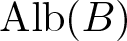 $\operatorname{Alb}(B)$ is non-trivial (which is equivalent to $H^0(T^*_{\mathbb{Z}} B) \neq 0$, since the $\mathbb{R}$-vector space $\operatorname{Hom}(H^0(T^*_{\mathbb{Z}} B), \mathbb{R})$ is zero if and only if the free $\mathbb{Z}$-module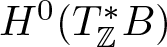 $H^0(T^*_{\mathbb{Z}} B)$ is zero), then $\operatorname{CH}_0(B)_{\hom}$ cannot be discrete. In other words, not all cycles of the same degree are equivalent to one another.
1.4. Connections to other work
As mentioned in Section 1.1, Theorem A can be thought of as a tropical version of Mumford’s theorem [Reference Mumford15] when  $\dim B = 2$ and Roitman’s generalization [Reference Roitman16] for arbitrary $\dim B \geq 2$. In fact, Mumford and Roitman’s results can be obtained as a corollary of Theorem A when $Y$ admits a tropicalization $B$, as long as one assumes that analytic curves tropicalize (see Remark 1.6).
To make this more precise, let us recall from [Reference Kontsevich, Soibelman, Etingof, Retakh and Singer10] that associated with any integral affine manifold  $B$, there is a rigid-analytic space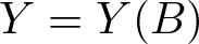 $Y = Y(B)$. Rigid-analytic spaces are the analogue of (complex) analytic spaces for non-archimedean fields. In our case, $Y$ is an analytic space over the Novikov field: this is the non-archimedean local field
 \begin{equation*}
\Lambda_{\Bbbk} = \left\lbrace \sum_{i=0}^\infty a_i T^{\lambda_i} \mid a_i \in \Bbbk, \lambda_i \in \mathbb{R}, \lim_{i\to \infty} \lambda_i = \infty \right\rbrace.
\end{equation*}
\begin{equation*}
\Lambda_{\Bbbk} = \left\lbrace \sum_{i=0}^\infty a_i T^{\lambda_i} \mid a_i \in \Bbbk, \lambda_i \in \mathbb{R}, \lim_{i\to \infty} \lambda_i = \infty \right\rbrace.
\end{equation*} The space  $Y$ comes with a projection $\pi:Y \to B$. We consider the natural surjective map
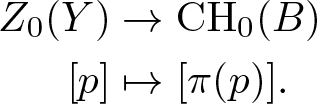 \begin{equation}
\begin{split}
Z_0(Y) &\to \operatorname{CH}_0(B)\\
[p] &\mapsto [\pi(p)].
\end{split}
\end{equation}
\begin{equation}
\begin{split}
Z_0(Y) &\to \operatorname{CH}_0(B)\\
[p] &\mapsto [\pi(p)].
\end{split}
\end{equation} If  $C \subset Y \times \mathbb{P}^{1}$ is a curve exhibiting some rational equivalence between points $(y_i^-)$ and $(y_i^+)$, under the assumption that analytic curves tropicalize the tropicalization $\pi(C)$ of $C$ is a tropical curve in $B \times \mathbb{R}$ exhibiting a tropical linear equivalence between the points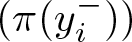 $(\pi(y_i^-))$ and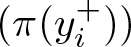 $(\pi(y_i^+))$ (in the sense of Definition 2.17). It follows that the map in Equation (3) descends to a map
 \begin{equation*}
\operatorname{CH}_0(Y) \to \operatorname{CH}_0(B).
\end{equation*}
\begin{equation*}
\operatorname{CH}_0(Y) \to \operatorname{CH}_0(B).
\end{equation*}Since this map is surjective, the commutative diagram
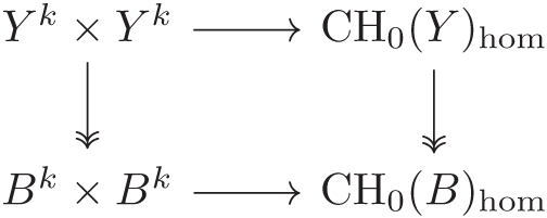
implies that if  $\operatorname{CH}_0(B)_{\hom}$ is infinite-dimensional then so is $\operatorname{CH}_0(Y)_{\hom}$.
Remark 1.5. Note that both Mumford and Roitman work with projective varieties. If  $Y = Z^{an}$ is the analytification of a projective variety $Z$, then by the rigid-analytic GAGA principle, one has that $\operatorname{CH}_*(Y) \cong \operatorname{CH}_*(Z)$ (the former group being built from analytic subvarieties, the latter from algebraic subvarieties). In this case, we recover Mumford and Roitman’s results. On the other hand, our result seems to be more general. For instance, when $Y$ is an (analytic) torus, its tropicalization is an integral affine torus. In this case, it is known that the projectivity of $Y$ translates into $B$ being polarized (this means it admits a strictly convex function with certain properties, cf. [Reference Mikhalkin and Zharkov13]). Our result works for general $B$ (not necessarily polarized) and would thus relate to the dimensionality of Chow groups of (non-algebraic) rigid-analytic varieties.
Remark 1.6. The fact that  $\pi(C)$ is a tropical curve whenever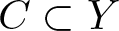 $C \subset Y$ is an irreducible analytic curve seems to be well-known to experts but has only appeared in the literature under certain assumptions, see [Reference Baker, Payne and Rabinoff3, Reference Tony Yue20].
Remark 1.7. The existence of non-realizable tropical curves (that is, tropical curves in  $B \times \mathbb{R}$ that do not admit a lift to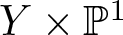 $Y \times \mathbb{P}^{1}$) could a priori suggest that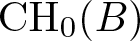 $\operatorname{CH}_0(B)$ should be ‘smaller’ than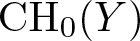 $\operatorname{CH}_0(Y)$ (as every relation in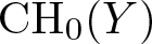 $\operatorname{CH}_0(Y)$ gives one in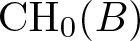 $\operatorname{CH}_0(B)$, but not the other way around). However, Theorem A shows that, even if smaller, these non-realizable tropical curves are not enough to make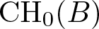 $\operatorname{CH}_0(B)$ finite-dimensional.
The results of Mumford were later translated into the world of symplectic geometry by Sheridan–Smith [Reference Sheridan and Smith18] and the corresponding generalization of Roitman by the present author in [Reference Muñiz-Brea14, Proposition 1.6], showing analogous statements for the so-called Lagrangian cobordism groups. All these works exploit a common idea (which goes back to the work of Severi): finding a dimension bound on a certain space by showing that it is isotropic for some differential form. We emphasize that, while our proof is based on the same method, it is not a direct translation of either Mumford or Roitman’s nor Sheridan–Smith’s proof. The former involves the study of differential forms on singular spaces and does not translate straightforwardly to tropical geometry, while the latter exploits a flexibility in Lagrangian cobordisms that is also not present in the tropical setting. Instead, we use the rigidity of tropical geometry and, in particular, tropical curves to give a purely tropical proof of our result.
One can also think of Proposition B as a (partial) tropical version of [Reference Bloch, Kas and Lieberman5]. The authors show that if  $Y$ is a smooth projective complex surface with Kodaira dimension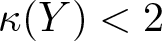 $\kappa(Y) \lt 2$, then the vanishing of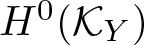 $H^0(\mathcal K_Y)$ implies $\operatorname{CH}_0(Y)_{\hom} \cong \operatorname{Alb}(Y)$ (in particular, $\operatorname{CH}_0(Y)_{\hom}$ is finite-dimensional). Bielliptic surfaces are examples of such surfaces, and they tropicalize to tropical Klein bottles; moreover, those of type I tropicalize to tropical Klein bottles of the type considered in this paper. Hence, Proposition B is the tropical version of the result in [Reference Bloch, Kas and Lieberman5] when $Y$ is an algebraic bielliptic surface of type I.
We lastly mention a connection between Proposition B and Lagrangian cobordism groups in symplectic geometry. If  $B$ is an integral affine manifold then one can consider the symplectic manifold $X(B):= T^*B / T^*_{\mathbb{Z}} B$ together with the Lagrangian torus fibration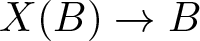 $X(B) \to B$. Points in $B$ correspond to Lagrangian torus fibres in $X(B)$, and the work of Sheridan–Smith [Reference Sheridan and Smith19] exhibits a relationship between (cylindrical) Lagrangian cobordisms between fibres of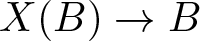 $X(B) \to B$ and tropical linear equivalence between points in $B$: showing that trivalent tropical curves admit Lagrangian lifts, they construct a map
 \begin{equation*}
\operatorname{CH}_0^{tri}(B) \to \operatorname{Cob}_{fib}(X(B))
\end{equation*}
\begin{equation*}
\operatorname{CH}_0^{tri}(B) \to \operatorname{Cob}_{fib}(X(B))
\end{equation*}for any integral affine manifold  $B$. (Here the superscript ‘tri’ means a tropical Chow group whose relations come only from trivalent tropical curves in $B \times \mathbb{R}$, and the subscript ‘fib’ means a Lagrangian cobordism group generated only by fibres of the fibration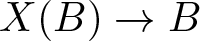 $X(B) \to B$.) For $B = K$ a tropical Klein bottle of type I and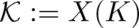 $\mathcal K:= X(K)$ the associated symplectic manifold, the subgroup
 \begin{equation*}
\operatorname{Cob}^{trop}(\mathcal K) \subset \operatorname{Cob}(\mathcal K)
\end{equation*}
\begin{equation*}
\operatorname{Cob}^{trop}(\mathcal K) \subset \operatorname{Cob}(\mathcal K)
\end{equation*}of the Lagrangian cobordism group of  $\mathcal K$ generated by tropical Lagrangians—that is, lifts of tropical subvarieties—was computed by the author in [Reference Muñiz-Brea14]. (Ref. [Reference Muñiz-Brea14] computes the planar cobordism group of $\mathcal K$, which is generally bigger than the cylindrical cobordism group. However, the other main theorem in that paper shows that the planar cobordism group is isomorphic to the Grothendieck group of the Fukaya category, and this isomorphism implies that the planar and cylindrical cobordism groups are actually isomorphic.) The subgroup $\operatorname{Cob}_{fib}(\mathcal K) \subset \operatorname{Cob}^{trop}(\mathcal K)$ generated by fibres was found to be isomorphic to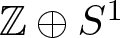 $\mathbb{Z} \oplus S^{1}$. (In [Reference Muñiz-Brea14], the Lagrangians and cobordisms are equipped with additional data, namely Pin and brane structures as well as a $G$-local system for a fixed abelian group $G$. The results in that paper compute the cobordism group including such data, hence the statement therein is $\operatorname{Cob}_{fib}(\mathcal K) \cong \mathbb{Z} \oplus (S^{1} \oplus G)$ (see [Reference Muñiz-Brea14, Proposition 4.25]). If one forgets local systems (or equivalently, if one sets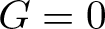 $G = 0$), then we obtain the above statement $\operatorname{Cob}_{fib}(\mathcal K) \cong \mathbb{Z} \oplus S^{1}$.) We thus see that the map
 \begin{align*}
\operatorname{CH}_0(K)\cong\operatorname{CH}_0^{tri}(K) &\to \operatorname{Cob}_{fib}(\mathcal K)\\
[p] &\mapsto [F_p]
\end{align*}
\begin{align*}
\operatorname{CH}_0(K)\cong\operatorname{CH}_0^{tri}(K) &\to \operatorname{Cob}_{fib}(\mathcal K)\\
[p] &\mapsto [F_p]
\end{align*}is an isomorphism. (The isomorphism  $\operatorname{CH}_0(K)\cong\operatorname{CH}_0^{tri}(K)$ follows from noting that all the tropical curves in the proof of Proposition B are trivalent.) In fact, in the present case, we have
Lemma 1.8. There is a well-defined map
 \begin{align*}
\operatorname{CH}_*(K) &\to \operatorname{Cob}^{trop}(\mathcal K)\\
V & \mapsto L_V
\end{align*}
\begin{align*}
\operatorname{CH}_*(K) &\to \operatorname{Cob}^{trop}(\mathcal K)\\
V & \mapsto L_V
\end{align*}mapping a tropical subvariety 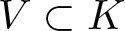 $V \subset K$ to the corresponding Lagrangian lift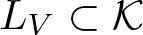 $L_V \subset \mathcal K$.
Proof. This map is well-defined on generators since (i) points (resp. the whole base) clearly lift to fibres (resp. the zero-section) and (ii) tropical curves are in this case tropical hypersurfaces, whose lift exists by results of Hicks [Reference Hicks7]. Furthermore, it also respects relations coming from tropical linear equivalence: for curves between points, this follows from the results of [Reference Sheridan and Smith19], whereas tropical surfaces in  $K \times \mathbb{R}$ between tropical curves in $K$ are tropical hypersurfaces and thus lift to Lagrangian surfaces in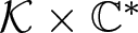 $\mathcal K \times \mathbb{C}^*$ (again by [Reference Hicks7]).
The computations of the tropical homology of a Klein bottle in [Reference Jell, Rau and Shaw9] together with Proposition B show:
Corollary 1.9. Let  $K$ be a tropical Klein bottle of type I. Then
 \begin{equation*}
\operatorname{CH}_*(K) \cong (\mathbb{Z} \oplus \operatorname{Alb}(K))\oplus(\mathbb{Z}^2 \oplus \mathbb{Z}_2 \oplus \operatorname{Pic}^0(K))\oplus \mathbb{Z}
\end{equation*}
\begin{equation*}
\operatorname{CH}_*(K) \cong (\mathbb{Z} \oplus \operatorname{Alb}(K))\oplus(\mathbb{Z}^2 \oplus \mathbb{Z}_2 \oplus \operatorname{Pic}^0(K))\oplus \mathbb{Z}
\end{equation*}with  $\operatorname{Alb}(K) \cong S^{1} \cong \operatorname{Pic}^0(K)$.
Proof. We consider the cycle-class map
 \begin{equation*}
\operatorname{CH}_i(K) \to H_{i,i}(K)
\end{equation*}
\begin{equation*}
\operatorname{CH}_i(K) \to H_{i,i}(K)
\end{equation*}where  $H_{i,j}(-)\equiv H_{i,j}(-;\mathbb{Z})$ denote the tropical homology groups [Reference Itenberg, Katzarkov, Mikhalkin and Zharkov8]. These maps are clearly surjective for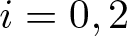 $i=0,2$. Furthermore, the tropical homology groups of $K$ have been computed for Klein bottles in [Reference Jell, Rau and Shaw9], and it was shown there that $H_{2,0}(K;\mathbb{R})=0$ and that this implies surjectivity for $i=1$. Thus, the cycle-class map is surjective on every degree, and we have a short exact sequence
 \begin{equation*}
0 \to \operatorname{CH}_*(K)_{\hom} \to \operatorname{CH}_*(K) \to H_{*,*}(K) \to 0.
\end{equation*}
\begin{equation*}
0 \to \operatorname{CH}_*(K)_{\hom} \to \operatorname{CH}_*(K) \to H_{*,*}(K) \to 0.
\end{equation*} We have that  $\operatorname{CH}_2(K)_{\hom} = 0$ and $\operatorname{CH}_1(K)_{\hom} = \operatorname{Pic}^0(K)$. By Proposition B, we also have $\operatorname{CH}_0(K)_{\hom} \cong \operatorname{Alb}(K)$. The result now follows by splitting the above short exact sequence and using the computation $H_{1,1}(K) \cong \mathbb{Z}^2 \oplus \mathbb{Z}_2$ from [Reference Jell, Rau and Shaw9].
Together with the main theorem of [Reference Muñiz-Brea14], this shows:
Proposition 1.10. The map  $\operatorname{CH}_*(K) \to \operatorname{Cob}^{trop}(\mathcal K)$ of Lemma 1.8 is an isomorphism.
Remark 1.11. As pointed out before Lemma 1.8, for this statement to hold, the Lagrangians in the group 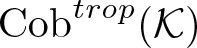 $\operatorname{Cob}^{trop}(\mathcal K)$ are not carrying a local system.
2. Preliminaries
Recall that an integral affine manifold is a smooth manifold  $B$ together with an integrable lattice $T_{\mathbb{Z}} B \subset TB$ of tangent vectors. This data is equivalent to an atlas of charts whose transition functions belong to the group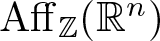 $\operatorname{Aff}_{\mathbb{Z}}(\mathbb{R}^n)$ of integral affine transformations of $\mathbb{R}^n$, i.e. those of the form
 \begin{equation*}
\mathbf{x} \mapsto A\mathbf{x} + \mathbf{x}_0, A \in \operatorname{GL}(n,\mathbb{Z}), \mathbf{x}_0 \in \mathbb{R}^n.
\end{equation*}
\begin{equation*}
\mathbf{x} \mapsto A\mathbf{x} + \mathbf{x}_0, A \in \operatorname{GL}(n,\mathbb{Z}), \mathbf{x}_0 \in \mathbb{R}^n.
\end{equation*} In this section, we introduce  $1$-dimensional tropical subvarieties of $B$ (so-called tropical curves), their moduli-spaces and deformations.
2.1. Background on tropical curves
We recall the notions of abstract tropical curves, tropical curves in a tropical manifold and parametrized tropical curves, following [Reference Mikhalkin11].
Given a tropical manifold  $B$, a tropical curve in $B$ is a weighted (In our definition, weights are non-negative.), balanced rational polyhedral complex of pure dimension one. We now define an intrinsic notion of a tropical curve (that is, with no reference to an ambient manifold $B$) and then identify tropical curves in $B$ with morphisms from these ‘abstract’ tropical curves to $B$.
$B$.
Let  $\Gamma$ be a graph, possibly with semi-infinite edges (Note that infinite edges, such as a graph with one edge and no vertices, are not allowed.) and no $1$-valent vertices. A tropical structure on $\Gamma$ is the data of a tropical affine structure on each of its edges such that the induced Riemannian metric $dx^2$—where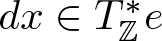 $dx \in T^*_{\mathbb{Z}} e$ is a generator—is complete. A graph $\Gamma$ together with a tropical structure will be called an abstract tropical curve.
Remark 2.1. When making statements that hold for any abstract tropical curve with underlying graph  $\Gamma$ (which we refer to as tropical curves whose topological type is that of $\Gamma$), we will use the notation $\Gamma$, with no reference to the metric structure.
Definition 2.2. Let  $B$ be a (non-necessarily compact) integral affine manifold. A parametrized tropical curve in $B$ is the data of an abstract tropical curve $\Gamma$ together with a proper embedding $h: \Gamma \to B$ such that:
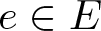
• its restriction to each edge is an integer affine map; that is, $dh(T_{\mathbb{Z}} e) \subset T_{\mathbb{Z}} B$ for all
$e\in E$;
$dh(T_{\mathbb{Z}} e) \subset T_{\mathbb{Z}} B$ for all
$e\in E$;• at each vertex
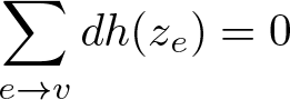
$v$ of
$\Gamma$, the balancing condition
(4)holds, where\begin{equation}
\sum_{e \to v} dh(z_e) = 0
\end{equation}
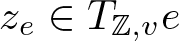
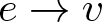
$z_e \in T_{\mathbb{Z},v} e$ is a primitive vector pointing outwards on the direction of
$e$. The notation
$e \to v$ in the summation means summing over all edges
$e$ which have
$v$ as one of their end vertices.






Two parametrized tropical curves  $h_i: \Gamma_i \to B, i =1,2$ are equivalent if there exists an isometry $f: \Gamma_1 \to \Gamma_2$ such that $h_1 = h_2 \circ f$.
The image  $h(\Gamma)$ of a parametrized tropical curve defines a tropical curve in $B$: the weight of (the image of) an edge $h(e)$ is the unique positive integer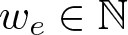 $w_e \in \mathbb{N}$ such that $dh(z_e) = w_e u_e$, where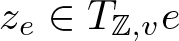 $z_e \in T_{\mathbb{Z},v} e$ and $u_e \in T_{\mathbb{Z},h(v)}B$ are both primitive vectors. Conversely, every tropical curve (that is, every weighted, balanced rational polyhedral complex of pure dimension one) can be parametrized in the sense of Definition 2.2, and such parametrization is unique. We will therefore use the terms tropical curve and parametrized tropical curve interchangeably.
Remark 2.3. Our definition of parametrized tropical curve is slightly different from that in [Reference Mikhalkin11, Definition 2.2], where the map  $h$ is not required to be an embedding and edges can be contracted to points. Clearly, every parametrized tropical curve in our sense is a parametrized tropical curve in the sense of [Reference Mikhalkin11]. Conversely, given a parametrized tropical curve in the sense of [Reference Mikhalkin11], there always exists (possibly after changing the underlying abstract tropical curve) a parametrized tropical curve in our sense with the same image in $B$. Since the end goal is to have a parametrized description of tropical curves in $B$, both definitions are equivalent in this sense. The main advantage of our definition is the following: given any tropical curve $C\subset B$, there exists a unique parametrized tropical curve (up to equivalence) with image $C$.
$C$.
We also introduce the following notation, which will be useful in later sections. Let 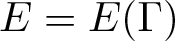 $E = E(\Gamma)$ be the set of edges of $\Gamma$ and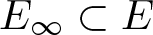 $E_\infty \subset E$ the set of semi-infinite edges. We denote by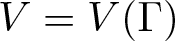 $V = V(\Gamma)$ the set of vertices of $\Gamma$ and by $\partial\Gamma$ the points at infinity of the unbounded edges of $\Gamma$. (That is,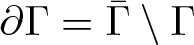 $\partial\Gamma= \bar{\Gamma}\setminus\Gamma$, where $\bar{\Gamma}$ is the compactification of $\Gamma$.) Choosing an orientation for each edge, we get maps
 \begin{equation}
v^\pm : E \to V \sqcup \partial\Gamma
\end{equation}
\begin{equation}
v^\pm : E \to V \sqcup \partial\Gamma
\end{equation}that assign to each edge its initial and final vertex.
2.2. Moduli of parametrized tropical curves
We denote by 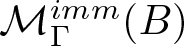 $\mathcal M_\Gamma^{imm}(B)$ the moduli-space of equivalence classes of immersed parametrized tropical curves in $B$ whose topological type is that of $\Gamma$ (that is, an element in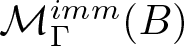 $\mathcal M_\Gamma^{imm}(B)$ is a map $h: \Gamma \to B$ satisfying the same conditions as in Definition 2.2 but which is only a proper immersion). Choosing an orientation on each edge gives a preferred generator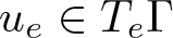 $u_e \in T_e\Gamma$ for each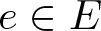 $e \in E$, which in turn yields an embedding
 \begin{equation}
\begin{split}
\mathcal M^{imm}_\Gamma(B) & \hookrightarrow B^{V}\times (T_{\mathbb{Z}} B\times (0,+\infty])^{E}\\
(h:\Gamma\to B) & \mapsto ((h(v))_{v\in V},(dh(u_e),len(h(e)))_{e\in E}).
\end{split}
\end{equation}
\begin{equation}
\begin{split}
\mathcal M^{imm}_\Gamma(B) & \hookrightarrow B^{V}\times (T_{\mathbb{Z}} B\times (0,+\infty])^{E}\\
(h:\Gamma\to B) & \mapsto ((h(v))_{v\in V},(dh(u_e),len(h(e)))_{e\in E}).
\end{split}
\end{equation} Here,  $len(h(e)) \in (0,+\infty]$ is the length of the interval $h(e)$.
Lemma 2.4. The above map gives 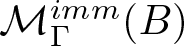 $\mathcal M^{imm}_\Gamma(B)$ the structure of a tropical affine manifold.
Proof. Recall that a choice of orientation on the edges also gives maps  $v^\pm : E \to V \cup \partial \Gamma$ recording the vertices of an edge $e$ (see Equation (5)). Given a point
 \begin{equation*}
(\mathbf{q},\mathbf{f},\mathbf{l}) = ((q_v)_{v \in V},(f_e,l_e)_{e \in E}) \in B^{V}\times (T_{\mathbb{Z}} B\times (0,+\infty])^{E},
\end{equation*}
\begin{equation*}
(\mathbf{q},\mathbf{f},\mathbf{l}) = ((q_v)_{v \in V},(f_e,l_e)_{e \in E}) \in B^{V}\times (T_{\mathbb{Z}} B\times (0,+\infty])^{E},
\end{equation*}we will use the notation 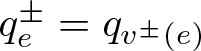 $q_e^\pm = q_{v^\pm(e)}$ to denote the values of $\mathbf q$ at the positions corresponding to the vertices of $e$. Also, for any point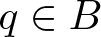 $q \in B$ and any tangent vector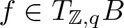 $f \in T_{\mathbb{Z},q}B$, we will denote by
 \begin{align*}
\gamma_{f,q}:\mathbb{R} \to B\\
\gamma_{f,q}(t) = q + t f
\end{align*}
\begin{align*}
\gamma_{f,q}:\mathbb{R} \to B\\
\gamma_{f,q}(t) = q + t f
\end{align*}the curve starting at  $q$ and with integral tangent vector $f$ (we parallel transport using the local system $T_{\mathbb{Z}} B$). Then the map above identifies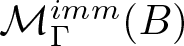 $\mathcal M^{imm}_\Gamma(B)$ with (an open subset of) the set of points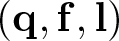 $ (\mathbf{q},\mathbf{f},\mathbf{l})$ such that:
(1)
$q^+_e = \gamma_{f_e,q^-_e}(l_e/w_e)$;(2)
$\sum_{e\to v} \pm w_e f_e=0$, where the
$\pm$ sign depends on whether
$e$ has been oriented as to point away from or into
$v$.




That is, the first condition ensures that the set of points  $\mathbf{q}$ can be joined by lines of integer slope (the slopes given by $\mathbf{f}$) and prescribed length, while the second guarantees that the balancing condition is met at each vertex, thus giving a tropical curve. Since the tangent space to (the image of)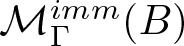 $\mathcal M_\Gamma^{imm}(B)$ is an integer affine subspace of $TB^V$, the result follows.
Remark 2.5. The moduli-space of tropical curves and its structure of a tropical affine manifold have appeared in the literature before, see e.g. [Reference Gathmann, Kerber and Markwig6] for the case 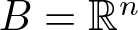 $B = \mathbb{R}^n$. We work with a different (local) embedding (compare our Equation (6) with [Reference Gathmann, Kerber and Markwig6, Proposition 4.7]) since it is more convenient for our purposes to remember the images of all the vertices of $\Gamma$ (see e.g. the proof of Proposition 3.3).
We now consider the restriction of the map (6) to  $\mathcal M_\Gamma(B) \subset \mathcal M^{imm}_\Gamma(B)$. Note this is now an embedding.
Corollary 2.6. The moduli-space 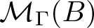 $\mathcal M_\Gamma(B)$ admits a tropical affine structure.
Proof. This follows from Lemma 2.4 together with the fact that  $\mathcal M_\Gamma(B) \subset \mathcal M^{imm}_\Gamma(B)$ is open.
2.3. Deformations of tropical curves
Let  $\Gamma$ be an abstract tropical curve.
Definition 2.7. The sheaf of locally constant  $1$-forms on $\Gamma$ is the sheaf
 \begin{equation*}
\mathcal T^*(U)=\left\lbrace\begin{array}{ll}
H^0(T^*_{\mathbb{Z}} e)\otimes\mathbb{R}, & U\subset e\\
\ker(f:\displaystyle\bigoplus_{e\to v} T_v^*e\to \mathbb{R}), & U \mathrm{neighbourhood\ of\ a\ vertex}\ v,
\end{array}\right.\!
\end{equation*}
\begin{equation*}
\mathcal T^*(U)=\left\lbrace\begin{array}{ll}
H^0(T^*_{\mathbb{Z}} e)\otimes\mathbb{R}, & U\subset e\\
\ker(f:\displaystyle\bigoplus_{e\to v} T_v^*e\to \mathbb{R}), & U \mathrm{neighbourhood\ of\ a\ vertex}\ v,
\end{array}\right.\!
\end{equation*}where  $f(\alpha_1,\dots,\alpha_k)=\sum_i \alpha_i(u_{e_i})$, $u_{e_i}$ being a primitive vector pointing outwards on the direction of $e_i$.
Remark 2.8. Note that, over an open set 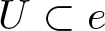 $U \subset e$, we have that $H^0(T^*_{\mathbb{Z}} e)\otimes\mathbb{R} \cong \mathbb{R}$, an isomorphism given by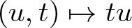 $(u, t) \mapsto tu$.
Example. Consider the curve  $\Gamma$ in Figure 2. Then any tuple of the form
 \begin{equation*}
(adx + bdy, -bdy, -adx) \in \bigoplus_{e_i \to v} T^*_v e_i, \quad a, b \in \mathbb{R}
\end{equation*}
\begin{equation*}
(adx + bdy, -bdy, -adx) \in \bigoplus_{e_i \to v} T^*_v e_i, \quad a, b \in \mathbb{R}
\end{equation*}is a section of  $\mathcal T$ over $U$, since $(adx + bdy)(u_1) -bdy(u_2) - adx(u_3) = 0$. Further, the restriction of $\mathcal T^*$ to an open set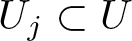 $U_j \subset U$ contained in the $j$-th vertex is just the projection $\oplus_{e_i \to v} T^*_v e_j \to T^*_v e_j \cong H^0(T^*_{\mathbb{Z}, v} e_j) \otimes \mathbb{R}$.
The following is a relative version of [Reference Sheridan and Smith19, Lemma 3.5] and [Reference Mikhalkin and Zharkov13, Lemma 6.1]. We use the notation introduced at the end of Section 2.1.
Lemma 2.10. There is an isomorphism  $H^0(\mathcal T^*)\cong H_1(\bar{\Gamma},\partial\Gamma;\mathbb{R})$.
Proof. Consider the linear map
 \begin{align*}
g:\mathbb{R}^E & \to \mathbb{R}^{V\sqcup\partial\Gamma} \to \mathbb{R}^V
\end{align*}
\begin{align*}
g:\mathbb{R}^E & \to \mathbb{R}^{V\sqcup\partial\Gamma} \to \mathbb{R}^V
\end{align*}given by composing  $1_e \mapsto 1_{v^+(e)} - 1_{v^-(e)}$ with the projection $\mathbb{R}^{V\sqcup\partial\Gamma} \to \mathbb{R}^V$, where $1_e$ is the generator of the $\mathbb{R}$-factor corresponding to $e$,
$e$,  $1_v$ is the generator of the $\mathbb{R}$-factor corresponding to $v$ and $v^\pm: E \to V\sqcup \partial\Gamma$ are the maps defined in Equation (5). First note that the group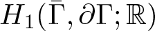 $H_1(\bar{\Gamma},\partial\Gamma;\mathbb{R})$ is canonically identified with the kernel of $g$ using simplicial homology. On the other hand, a choice of orientation for the edges of $\Gamma$ gives preferred generators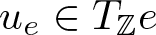 $u_e \in T_{\mathbb{Z}} e$ and hence preferred isomorphisms $H^0(T^*_{\mathbb{Z}} e) \otimes \mathbb{R} \cong \mathbb{R}$. It is then clear that an element of $\oplus_e H^0(T^*_{\mathbb{Z}} e) \otimes \mathbb{R}$ extends to a global section of $\mathcal T^*$—that is, it is in the kernel of $f$—if and only if the corresponding element in $\mathbb{R}^E$ lies in the kernel of $g$.
$g$.
Remark 2.11. Using a simplicial model for 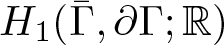 $H_1(\bar{\Gamma},\partial\Gamma;\mathbb{R})$, an explicit isomorphism $\eta:\mathcal T^*(\Gamma) \xrightarrow{\sim}H_1(\bar{\Gamma},\partial\Gamma;\mathbb{R})$ is given by sending a $1$-form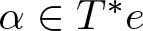 $\alpha\in T^*e$ to the $1$-chain $\alpha(u_e)e \in C_1^{simp}(\bar{\Gamma};\mathbb{R})$, where $u_e$ is a primitive vector in $T_{\mathbb{Z}} e$ whose direction is determined by the orientation of $e$.
$e$.
A tropical curve (in red) together with a collection of primitive integral vectors, one for each edge, pointing outwards.
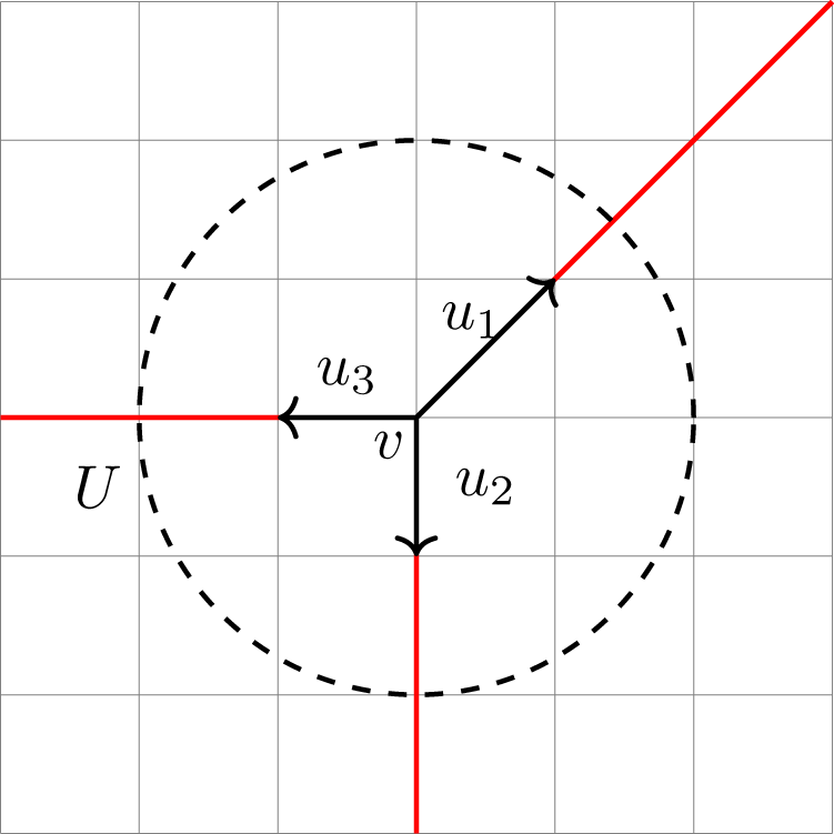
Figure 2 Long description
The diagram features a tropical curve represented by a red line intersecting a dashed circle. The circle is centered on a grid and three black vectors labeled u1, u2 and u3 extend from a central point labeled v. Each vector points outward from the center of the circle. The vector u1 is directed towards the upper right, u2 points downward and u3 extends to the left. The red curve labeled U intersects the circle at two points, one on the left and one at the top right, continuing beyond the circle's boundary. The dashed circle serves as a boundary for the vectors, emphasizing their outward direction from the center.
Now let  $h:\Gamma\to B$ be a parametrized tropical curve in $B$; for simplicity, we will refer to it as $\Gamma$, even though the map $h$ is part of the definition.
Definition 2.12. The sheaf of deformations of  $\Gamma$ is the sheaf
 \begin{equation*}
\mathcal D(U)=\left\lbrace
\begin{array}{ll}
T_p B/T_p h(e), & p \in U\subset e\\
T_vB, & U \mathrm{neighbourhood\ of\ the\ vertex}\ v
\end{array}
\right..
\end{equation*}
\begin{equation*}
\mathcal D(U)=\left\lbrace
\begin{array}{ll}
T_p B/T_p h(e), & p \in U\subset e\\
T_vB, & U \mathrm{neighbourhood\ of\ the\ vertex}\ v
\end{array}
\right..
\end{equation*} Note that there are canonical isomorphisms  $T_p B/T_p h(e) \cong T_q B/T_q h(e)$ for any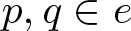 $p,q \in e$ given by parallel transport, hence the sheaf is well-defined. The restriction maps are given by the projections $T_v B\to T_vB/T_v e \cong T_pB/T_p e$, the latter isomorphism given again by parallel transport. A deformation of $\Gamma$ is a section of $\mathcal D$, and we write $\operatorname{def}(\Gamma) := H^0(\mathcal D)$ for the group of (global) deformations.
Example. Consider again the tropical curve in Figure 2. The vector 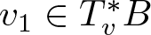 $v_1 \in T^*_v B$ is a section of $\mathcal D(U)$. The restriction to an open set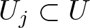 $U_j \subset U$ contained in the $j$-th edge is just its equivalence class $[v_1] \in T_v B / T_v e_j$, which can be thought of as the projection of $v_1$ to an orthogonal complement to $e_j$. The same applies to $v_2$ and $v_3$.
Lemma 2.14. There is an identification  $T_h \mathcal M_\Gamma(B) \cong \operatorname{def}(\Gamma)$.
Proof. A deformation of  $\Gamma$—that is, a global section of $\mathcal D$—is determined by its stalks on the vertices; that is, by an element
 \begin{equation*}
(u_v)_{v\in V} \in \oplus_v T_v B.
\end{equation*}
\begin{equation*}
(u_v)_{v\in V} \in \oplus_v T_v B.
\end{equation*} Such a tuple determines a deformation if and only if  $[u_{v^+(e)}] = [u_{v^-(e)}] \in TB/Te$ for every edge $e$.
$e$.
Let us now show how to view 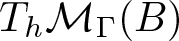 $T_h\mathcal M_\Gamma(B)$ as the same subset of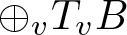 $\oplus_v T_v B$. Recall from the proof of Lemma 2.4 that the embedding (6) identifies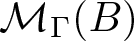 $\mathcal M_\Gamma(B)$ with (an open subset of) the set of points
 \begin{equation*}
(\mathbf{q},\mathbf{f},\mathbf{l}) = ((q_v)_{v \in V},(f_e,l_e)_{e \in E}) \in B^{V}\times (T_{\mathbb{Z}} B\times (0,+\infty])^{E},
\end{equation*}
\begin{equation*}
(\mathbf{q},\mathbf{f},\mathbf{l}) = ((q_v)_{v \in V},(f_e,l_e)_{e \in E}) \in B^{V}\times (T_{\mathbb{Z}} B\times (0,+\infty])^{E},
\end{equation*}such that:
(1)
$q^+_e = \gamma_{f_e,q^-_e}(l_e/w_e)$;(2)
$\sum_{e\to v} \pm w_e f_e=0$, where the
$\pm$ sign depends on whether
$e$ has been oriented as to point away from or into
$v$.




Here,  $q_e^\pm$ are the ends of an edge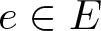 $e \in E$ and $\gamma_{f_e,q_e^-}: \mathbb{R} \to B$ is the curve whose tangent vector is (the parallel transport of)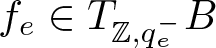 $f_e \in T_{\mathbb{Z},q_e^-} B$ and such that $\gamma_{f_e,q_e^-}(0) = q_e^-$. In particular, note that the projection
 \begin{equation*}
\mathcal M_\Gamma(B) \hookrightarrow B^{V}\times (T_{\mathbb{Z}} B\times (0,+\infty])^{E} \to B^V
\end{equation*}
\begin{equation*}
\mathcal M_\Gamma(B) \hookrightarrow B^{V}\times (T_{\mathbb{Z}} B\times (0,+\infty])^{E} \to B^V
\end{equation*}is a local embedding (once the position of the vertices is known, the curve is fixed). It follows that we can identify 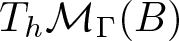 $T_h\mathcal M_\Gamma(B)$ with a subset of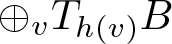 $\oplus_{v} T_{h(v)} B$. Lastly, given $(u_v)_{v \in V} \in \oplus_{v} T_{h(v)} B$, condition 1. above is equivalent to $[u_{v^+(e)}] = [u_{v^-(e)}] \in TB/Te$ for every edge $e$. Indeed, once we perturb $v^-(e)$ via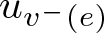 $u_{v^-(e)}$, the fact that $v^\pm(e)$ are connected by a curve of direction $f_e$ implies that $u_{v^+(e)} = u_{v^-(e)} + \lambda f_e$, where $\lambda = 0$ if and only if the perturbed edge keeps the same length (see Figure 3).
Two types of deformations of a tropical curve. On the left, we have deformations where  $u_{v^-(e)} = u_{v^+(e)} \in TB$, i.e. translations of the curve. On the right we have deformations where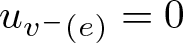 $u_{v^-(e)}=0$ and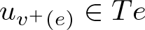 $u_{v^+(e)} \in Te$ (in particular, $[u_{v^-(e)}] = [u_{v^+(e)}] = 0 \in TB/Te$). These deformations expand (or contract) one edge. Similarly, one could have deformations with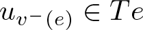 $u_{v^-(e)}\in Te$ and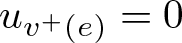 $u_{v^+(e)} = 0$.
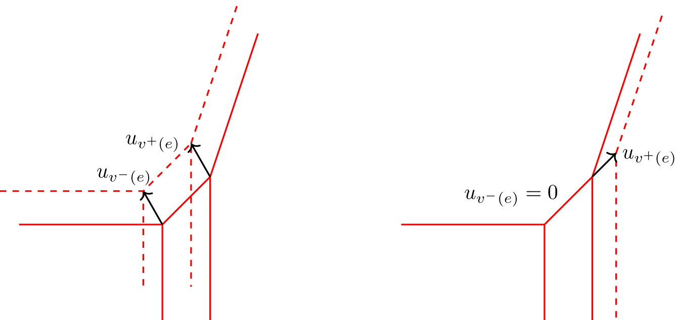
Figure 3 Long description
The image consists of two sections, each illustrating a different type of deformation of a tropical curve. On the left, the diagram shows a curve with two vectors labeled as u subscript v superscript minus left parenthesis e right parenthesis and u subscript v superscript plus left parenthesis e right parenthesis. These vectors are represented by arrows pointing along the curve, indicating a deformation where both vectors are non-zero. The curve is depicted with solid and dashed lines, suggesting a change in position or direction. On the right, the diagram shows a similar curve with the vector u subscript v superscript minus left parenthesis e right parenthesis set to zero, while u subscript v superscript plus left parenthesis e right parenthesis remains non-zero. This indicates a deformation where one edge is contracted or remains unchanged. The solid and dashed lines again suggest a change in the curve's configuration. Both sections use red lines to represent the curves and black arrows for the vectors, emphasizing the deformation process.
We have defined two sheaves: the sheaf  $\mathcal T^*$ of locally constant $1$-forms and the sheaf $\mathcal D$ of deformations. The following Lemma relates the two sheaves:
Lemma 2.15. For every locally constant 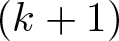 $(k+1)$-form $\omega \in H^0(\wedge^{k+1}T^*B)$, the map
 \begin{align*}
\wedge^k T_v B &\to \oplus_{e \to v} T_v^*e\\
u& \mapsto (w_e\iota_u \omega)_{e\to v}
\end{align*}
\begin{align*}
\wedge^k T_v B &\to \oplus_{e \to v} T_v^*e\\
u& \mapsto (w_e\iota_u \omega)_{e\to v}
\end{align*}extends to a sheaf homomorphism
 \begin{equation*}
\Phi_\omega: \wedge^{k}\mathcal D \to \mathcal T^*.
\end{equation*}
\begin{equation*}
\Phi_\omega: \wedge^{k}\mathcal D \to \mathcal T^*.
\end{equation*} Here we denote by  $\iota_u \omega = \omega(u\wedge-)$ the contraction of $\omega$ with $u$.
$u$.
Proof. The map is clearly compatible with restriction. Hence, it is enough to show that  $(w_e\iota_u \omega)_{e\to v} \in \ker(f)$ (cf. Definition 2.7). This follows from the balancing condition: if $u = u_1\wedge\dots\wedge u_k \in \wedge^kT_vB$, then one has
 \begin{equation*}
f((w_e\iota_u \omega)_{e\to v}) = \sum_{e\to v} w_e \omega(u\wedge u_{e}) = \omega(u\wedge \sum_{e\to v} w_e u_{e}) = 0
\end{equation*}
\begin{equation*}
f((w_e\iota_u \omega)_{e\to v}) = \sum_{e\to v} w_e \omega(u\wedge u_{e}) = \omega(u\wedge \sum_{e\to v} w_e u_{e}) = 0
\end{equation*}since  $\sum_{e\to v} w_e u_{e} = 0$.
Putting together Lemmas 2.10 and 2.15, we obtain a map
 \begin{equation*}
\wedge^k \text{def}(\Gamma) = \wedge^k H^0(\mathcal D) \to H^0(\mathcal T^*) \cong H_1(\bar{\Gamma},\partial\Gamma;\mathbb{R}).
\end{equation*}
\begin{equation*}
\wedge^k \text{def}(\Gamma) = \wedge^k H^0(\mathcal D) \to H^0(\mathcal T^*) \cong H_1(\bar{\Gamma},\partial\Gamma;\mathbb{R}).
\end{equation*}2.4. Tropical linear equivalence
We now introduce a particular type of tropical curves in  $B \times \mathbb{R}$; these will be used to define the equivalence relation of tropical linear equivalence (see Definition 2.17). From now on, we assume that $B$ is compact.
Definition 2.16. We say that a parametrized tropical curve  $h:\Gamma \to B \times \mathbb{R}$ is horizontal at infinity if the composition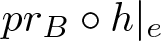 $pr_B \circ h|_{e}$ is a constant map for every semi-infinite edge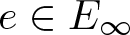 $e \in E_\infty$.
We denote by  $\mathcal M^{hor}_\Gamma (B \times \mathbb{R}) \subset \mathcal M_\Gamma (B \times \mathbb{R})$ the moduli-space of parametrized tropical curves $h: \Gamma \to B \times \mathbb{R}$ which are horizontal at infinity (that is, those tropical curves in $B \times \mathbb{R}$ that are horizontal at infinity and whose topological type is that of $\Gamma$). Then it follows from Definition 2.16 that there are well-defined maps
 \begin{equation}
\begin{split}
ev_{\pm\infty}: \mathcal M^{hor}_\Gamma (B \times \mathbb{R}) &\to \prod_{e\in E_{\pm\infty}} B^{w_e}\\
h &\mapsto ((pr_B \circ h(e))^{w_e})_{e \in E_{\pm\infty}}
\end{split}
\end{equation}
\begin{equation}
\begin{split}
ev_{\pm\infty}: \mathcal M^{hor}_\Gamma (B \times \mathbb{R}) &\to \prod_{e\in E_{\pm\infty}} B^{w_e}\\
h &\mapsto ((pr_B \circ h(e))^{w_e})_{e \in E_{\pm\infty}}
\end{split}
\end{equation}that record the images, with multiplicity, of the semi-infinite edges of  $\Gamma$ asymptotic to $\pm\infty$. Here, we used the notation $b^n := (b,\dots,b) \in B^n$ for $b \in B$ and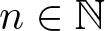 $n \in \mathbb{N}$, and we decompose $E_\infty = E_{-\infty} \cup E_{+\infty}$ depending on whether (the image of) an edge is asymptotic to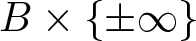 $B \times \{\pm \infty\}$.
Note that the balancing condition implies that  $\sum_{e \in E_{\pm\infty}} \pm w_e = 0$ (see [Reference Allermann, Hampe and Rau1, Proposition 3.2, (e)] for a proof, together with Lemma 2.18), hence the maps $ev_{-\infty}$ and $ev_\infty$ have as target a common $B^n$. Composing $(ev_{-\infty},ev_{+\infty})$ with the map
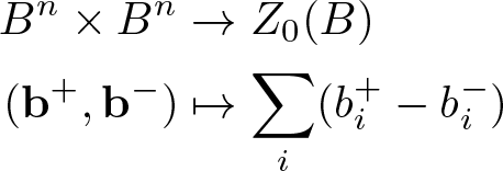 \begin{equation}
\begin{split}
B^n \times B^n &\to Z_0(B)\\
(\mathbf{b}^+,\mathbf{b}^-) &\mapsto \sum_i (b_i^+ - b_i^-)
\end{split}
\end{equation}
\begin{equation}
\begin{split}
B^n \times B^n &\to Z_0(B)\\
(\mathbf{b}^+,\mathbf{b}^-) &\mapsto \sum_i (b_i^+ - b_i^-)
\end{split}
\end{equation}yields a map
 \begin{equation*}
\mathcal M^{hor}_\Gamma (B \times \mathbb{R}) \to Z_0(B).
\end{equation*}
\begin{equation*}
\mathcal M^{hor}_\Gamma (B \times \mathbb{R}) \to Z_0(B).
\end{equation*} Let  $R_0(B) \subset Z_0(B)$ be the subgroup generated by the image of $\cup_\Gamma \mathcal M^{hor}_\Gamma(B \times \mathbb{R}) \to Z_0(B)$.
Definition 2.17. We say  $0$-cycles $V_\pm \in Z_0(B)$ are (tropically) linearly equivalent if $V_+ - V_- \in R_0(B)$. (Roughly speaking, one can think of two cycles $V_\pm$ being tropically linearly equivalent if there exists a tropical curve $h:\Gamma \to B \times \mathbb{R}$ which coincides with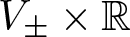 $V_\pm \times \mathbb{R}$ on a neighbourhood of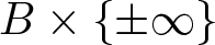 $B \times \{\pm\infty\}$. This is, however, not precise: for instance, the cycles $V_\pm$ could be tropically linearly equivalent because there is a tropical curve $h:\Gamma \to B \times \mathbb{R}$ which coincides with $(V_\pm \cup W)\times \mathbb{R}$ on a neighbourhood of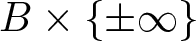 $B \times \{\pm\infty\}$ for some set of points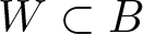 $W \subset B$, but a curve coinciding with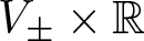 $V_\pm \times \mathbb{R}$ need not exist.) The tropical $0$-th Chow group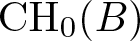 $\operatorname{CH}_0(B)$ is the quotient
 \begin{equation*}
\operatorname{CH}_0(B) =Z_0(B)/R_0(B).
\end{equation*}
\begin{equation*}
\operatorname{CH}_0(B) =Z_0(B)/R_0(B).
\end{equation*}Although this definition seems different from Definition 1.2, we have:
Lemma 2.18. Let 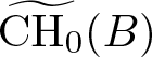 $\widetilde{\operatorname{CH}_0}(B)$ be the Chow group obtained with the definition of rational equivalence in Definition 1.2. Then there is an isomorphism $\widetilde{\operatorname{CH}_0}(B) \cong\operatorname{CH}_0(B)$.
Proof. The proof is identical to that in [Reference Allermann, Hampe and Rau1, Proposition 3.5] and uses the ‘full graph’ construction of [Reference Mikhalkin12] (also named ‘tropical graph cobordism’ in [Reference Allermann and Rau2]), see Figure 4.
In the remainder of this paper, we will use Definition 2.17, as it is more convenient for our proofs.
Schematic picture of full graph construction. Given a function 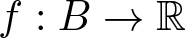 $f : B \to \mathbb{R}$ (whose graph we represent on the left), the full graph construction extends its bending locus towards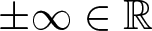 $\pm\infty\in \mathbb{R}$, creating a curve that is horizontal at infinity.
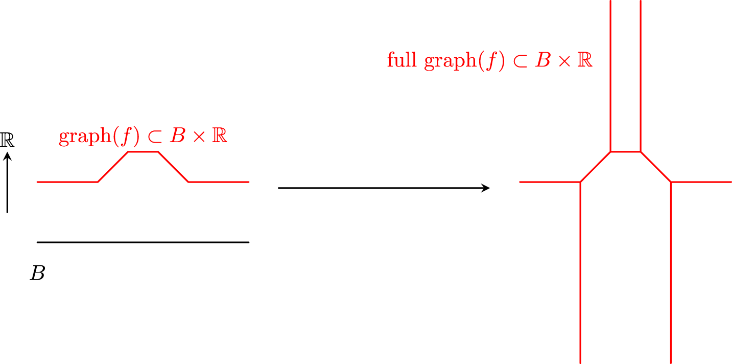
Figure 4 Long description
The image shows two panels connected by a rightward-pointing black arrow. The left panel contains a red piecewise polyline positioned above a horizontal black line. The horizontal black line is labeled B below it. A vertical black axis is shown on the left side, labeled R with an upward arrow. The red polyline has several connected diagonal and horizontal segments. Above the red polyline, the label reads: graph of f is a subset of B cross R. A black horizontal arrow points from the left panel to the right panel. The right panel shows a red outlined shape consisting of vertical red line segments and horizontal red line segments forming a connected region. The shape has vertical sides extending upward and downward and horizontal extensions pointing left and right at two levels, connected by a central vertical segment. Above this shape, the label reads: full graph of f is a subset of B cross R. The left panel shows a single red polyline above a base line, while the right panel shows a thickened red outlined region with multiple vertical and horizontal segments extending outward.
3. Tropical forms and dimensionality of tropical Chow groups
3.1. Infinite dimensionality
Let  $\Psi: B^{2n} \to \operatorname{CH}_0(B)$ be the composition of the map in Equation (8) with the projection $Z_0(B) \to \operatorname{CH}_0(B)$; that is, $\Psi$ is the map defined by
 \begin{equation*}
\Psi(\mathbf{b}^+,\mathbf{b}^-) = \sum_{i=1}^n ([b^+_i] - [b^-_i]),
\end{equation*}
\begin{equation*}
\Psi(\mathbf{b}^+,\mathbf{b}^-) = \sum_{i=1}^n ([b^+_i] - [b^-_i]),
\end{equation*}where  $\mathbf{b}^\pm = (b^\pm_1,\dots,b^\pm_n) \in B^n$. We consider the subset ${\mathcal Z_{n,k}}\subset B^{2n}\times B^{2k}$ defined as
 \begin{equation*}
{\mathcal Z_{n,k}}:=\left\lbrace{(\mathbf{b}^+,\mathbf{b}^-,\mathbf{c}^+,\mathbf{c}^-) \,\vert\, \Psi(\mathbf{b}^+,\mathbf{b}^-)=\Psi(\mathbf{c}^+,\mathbf{c}^-)}\right\rbrace.
\end{equation*}
\begin{equation*}
{\mathcal Z_{n,k}}:=\left\lbrace{(\mathbf{b}^+,\mathbf{b}^-,\mathbf{c}^+,\mathbf{c}^-) \,\vert\, \Psi(\mathbf{b}^+,\mathbf{b}^-)=\Psi(\mathbf{c}^+,\mathbf{c}^-)}\right\rbrace.
\end{equation*} To elucidate the structure of  $\mathcal Z_{n,k}$, we will need the following two Lemmas:
Lemma 3.1. If  $(\mathbf{b}^+,\mathbf{b}^-,\mathbf{c}^+,\mathbf{c}^-) \in {\mathcal Z_{n,k}}$, then there exist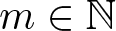 $m \in \mathbb{N}$,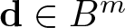 $\mathbf{d} \in B^{m}$ and a parametrized tropical curve $h:\Gamma \to B \times \mathbb{R}$ such that
 \begin{equation}
\begin{split}
(ev_{-\infty}, ev_{\infty})(\Gamma)
=
(\mathbf{b}^- \cup \mathbf{c}^- \cup \mathbf{d}, \mathbf{b}^+ \cup \mathbf{c}^+ \cup \mathbf{d})
\in
B^{n+k+m} \times B^{n+k+m}.
\end{split}
\end{equation}
\begin{equation}
\begin{split}
(ev_{-\infty}, ev_{\infty})(\Gamma)
=
(\mathbf{b}^- \cup \mathbf{c}^- \cup \mathbf{d}, \mathbf{b}^+ \cup \mathbf{c}^+ \cup \mathbf{d})
\in
B^{n+k+m} \times B^{n+k+m}.
\end{split}
\end{equation} Here, the maps  $ev_{\pm\infty}$ are those defined in Equation (7).
Proof. Let  $(\mathbf{b}^+,\mathbf{b}^-,\mathbf{c}^+,\mathbf{c}^-) \in {\mathcal Z_{n,k}}$. This means there exist tropical curves $h_i : \Gamma_i \to B \times \mathbb{R}$ which are horizontal at infinity and such that
 \begin{equation*}
\prod_i (ev_{-\infty}, ev_{\infty})(\Gamma_{i})
=
(\mathbf{b}^- \cup \mathbf{c}^- \cup \mathbf{d}, \mathbf{b}^+ \cup \mathbf{c}^+ \cup \mathbf{d})
\subset
B^{n+k+m} \times B^{n+k+m}.
\end{equation*}
\begin{equation*}
\prod_i (ev_{-\infty}, ev_{\infty})(\Gamma_{i})
=
(\mathbf{b}^- \cup \mathbf{c}^- \cup \mathbf{d}, \mathbf{b}^+ \cup \mathbf{c}^+ \cup \mathbf{d})
\subset
B^{n+k+m} \times B^{n+k+m}.
\end{equation*}for some 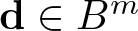 $\mathbf{d}\in B^{m}$. Indeed, note that $(\mathbf{b}^+,\mathbf{b}^-,\mathbf{c}^+,\mathbf{c}^-) \in {\mathcal Z_{n,k}}$ means that $\sum_i b^+_i + \sum_i c^+_i \sim \sum_i b^-_i + \sum_i c^-_i$ in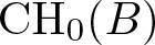 $\operatorname{CH}_0(B)$, and relations in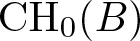 $\operatorname{CH}_0(B)$ are, by definition, generated tropical curves that are horizontal at infinity. Note that the union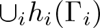 $\cup_i h_i(\Gamma_i)$ is a tropical curve in $B \times \mathbb{R}$. We argued in Section 2.1 that every tropical curve admits a parametrization: hence, there exists a parametrized tropical curve $h: \Gamma \to B \times \mathbb{R}$ with $h(\Gamma) = \cup_i h_i(\Gamma_i)$.
Lemma 3.2. Let  $\Gamma$ be an abstract tropical curve. Then the image of the evaluation map
 \begin{equation*}
(ev_{-\infty}, ev_{\infty}): \mathcal M^{hor}_\Gamma(B \times \mathbb{R}) \to B^{d} \times B^{d}
\end{equation*}
\begin{equation*}
(ev_{-\infty}, ev_{\infty}): \mathcal M^{hor}_\Gamma(B \times \mathbb{R}) \to B^{d} \times B^{d}
\end{equation*}is a countable union of open subsets of affine subspaces.
Proof. Recall from Corollary 2.6 that  $\mathcal M^{hor}_\Gamma(B\times\mathbb{R}) \subset \mathcal M^{hor,imm}_\Gamma(B\times\mathbb{R})$ can be realized as (an open subset of) an integral affine submanifold of $(B\times \mathbb{R})^V \times (T_{\mathbb{Z}}(B\times \mathbb{R})\times(0,+\infty])^E$ via the map in Equation (6). (Strictly speaking, we have only proved this for $\mathcal M_\Gamma(B\times\mathbb{R}) \subset \mathcal M_\Gamma^{imm}(B \times \mathbb{R})$. However, note that $\mathcal M^{hor}_\Gamma(B\times\mathbb{R}) \subset \mathcal M_\Gamma(B\times\mathbb{R})$ is the intersection of $\mathcal M_\Gamma(B\times\mathbb{R})$ with the submanifold of $(B\times \mathbb{R})^V \times (T_{\mathbb{Z}}(B\times\mathbb{R}) \times (0,+\infty])^E$ whose projection to $T_{\mathbb{Z}}(B\times \mathbb{R})^{E_\infty}$ lies in $T_{\mathbb{Z}} B \subset T_{\mathbb{Z}}(B\times \mathbb{R})$. This shows that $\mathcal M^{hor}_\Gamma(B\times\mathbb{R})$ is still an integral affine submanifold of $(B\times \mathbb{R})^V \times (T_{\mathbb{Z}}(B\times\mathbb{R}) \times (0,+\infty])^E$.) This map gives $\mathcal M^{hor}_\Gamma(B\times\mathbb{R})$ its tropical affine structure, and the map $(ev_{-\infty}, ev_{\infty}): \mathcal M^{hor}_\Gamma(B \times \mathbb{R}) \to B^{d} \times B^{d}$ is identified with the projection
 \begin{equation*}
(B\times\mathbb{R})^{V}\times (T_{\mathbb{Z}}(B\times \mathbb{R})\times (0,+\infty])^{E} \to (B\times\mathbb{R})^{V_{\infty}},
\end{equation*}
\begin{equation*}
(B\times\mathbb{R})^{V}\times (T_{\mathbb{Z}}(B\times \mathbb{R})\times (0,+\infty])^{E} \to (B\times\mathbb{R})^{V_{\infty}},
\end{equation*}where  $V_{\infty}$ is the set of vertices from which the unbounded edges emanate. Since projecting is an affine map, and $\mathcal M_\Gamma^{hor}(B\times\mathbb{R})$ is an affine subspace, the result follows.
We can now show:
Proposition 3.3. The set  ${\mathcal Z_{n,k}}$ is a countable union of open subsets of affine subspaces of $B^{2n} \times B^{2k}$.
Proof. For each 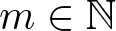 $m \in \mathbb{N}$, we consider the space
 \begin{equation*}
\mathcal M^{hor}(B\times\mathbb{R})_m = \bigcup_{|E(\Gamma)_\infty| = 2n+2k+2m} \mathcal M^{hor}_\Gamma(B \times \mathbb{R}),
\end{equation*}
\begin{equation*}
\mathcal M^{hor}(B\times\mathbb{R})_m = \bigcup_{|E(\Gamma)_\infty| = 2n+2k+2m} \mathcal M^{hor}_\Gamma(B \times \mathbb{R}),
\end{equation*}where the union ranges over all topological types with  $2n+2k+2m$ semi-infinite edges. Let
 \begin{equation*}
\mathcal M^{hor}(B\times\mathbb{R})_m^{\mathcal Z_{n,k}} \subset \mathcal M^{hor}(B\times\mathbb{R})_m
\end{equation*}
\begin{equation*}
\mathcal M^{hor}(B\times\mathbb{R})_m^{\mathcal Z_{n,k}} \subset \mathcal M^{hor}(B\times\mathbb{R})_m
\end{equation*}be the subset of curves  $\Gamma \in \mathcal M^{hor}(B\times\mathbb{R})_m$ that satisfy Equation (9) (that is, they have $n + k + m$ ends at each $\pm \infty$, and $m$ of the asymptotic points coincide on both ends). Note that $\mathcal M^{hor}(B\times\mathbb{R})_m^{\mathcal Z_{n,k}}$ admit maps $\mathcal M^{hor}(B\times\mathbb{R})^{\mathcal Z_{n,k}}_m \to {\mathcal Z_{n,k}}$ by composing
 \begin{equation}
\mathcal M^{hor}(B\times\mathbb{R})^{\mathcal Z_{n,k}}_m \xrightarrow{(ev_{-\infty}, ev_{\infty})} B^{n+k+m} \times B^{n+k+m} \to \mathcal Z_{n,k} \subset B^{2n} \times B^{2k},
\end{equation}
\begin{equation}
\mathcal M^{hor}(B\times\mathbb{R})^{\mathcal Z_{n,k}}_m \xrightarrow{(ev_{-\infty}, ev_{\infty})} B^{n+k+m} \times B^{n+k+m} \to \mathcal Z_{n,k} \subset B^{2n} \times B^{2k},
\end{equation}where the second map is the product of the projections  $B^{n+m+k} \to B^{n+m}$ (with a final reordering of factors $B^{n+m} \times B^{n+m} \to B^{2n} \to B^{2m}$). Furthermore, Lemma 3.1 shows that the union of these maps
 \begin{equation*}
\bigcup_m \mathcal M^{hor}(B\times\mathbb{R})^{\mathcal Z_{n,k}}_m \to \mathcal Z_{n,k} \subset B^{2n} \times B^{2k}.
\end{equation*}
\begin{equation*}
\bigcup_m \mathcal M^{hor}(B\times\mathbb{R})^{\mathcal Z_{n,k}}_m \to \mathcal Z_{n,k} \subset B^{2n} \times B^{2k}.
\end{equation*}surjects onto  $\mathcal Z_{n,k}$. Note that this is a countable union, hence it is enough to show that the images of the maps $\mathcal M^{hor}(B\times\mathbb{R})^{\mathcal Z_{n,k}}_m \to B^{2n} \times B^{2k}$ satisfy the statement of the proposition. Since the second map in Equation (10) is a projection, which is affine, we can further reduce to showing that the image of the evaluation maps
 \begin{equation*}
(ev_{-\infty}, ev_{\infty}): \mathcal M^{hor}(B \times \mathbb{R})_m^{\mathcal Z_{n,k}} \to B^{n+m+k} \times B^{n+m+k}
\end{equation*}
\begin{equation*}
(ev_{-\infty}, ev_{\infty}): \mathcal M^{hor}(B \times \mathbb{R})_m^{\mathcal Z_{n,k}} \to B^{n+m+k} \times B^{n+m+k}
\end{equation*}satisfy the statement of the proposition.
First note that this is true for the extended map
 \begin{equation*}
(ev_{-\infty},ev_\infty):\mathcal M^{hor}(B \times \mathbb{R})_m \to B^{n+m+k} \times B^{n+m+k}
\end{equation*}
\begin{equation*}
(ev_{-\infty},ev_\infty):\mathcal M^{hor}(B \times \mathbb{R})_m \to B^{n+m+k} \times B^{n+m+k}
\end{equation*} (note we now consider  $\mathcal M^{hor}(B \times \mathbb{R})_m$ instead of $\mathcal M^{hor}(B \times \mathbb{R})_m^{\mathcal Z_{n,k}}$ as the domain). Indeed, the moduli-space $\mathcal M^{hor}(B\times \mathbb{R})_m$ and the above map are defined as a countable union, and each piece
 \begin{equation*}
\mathcal M_\Gamma^{hor}(B \times \mathbb{R}) \to B^{n+m+k} \times B^{n+m+k}
\end{equation*}
\begin{equation*}
\mathcal M_\Gamma^{hor}(B \times \mathbb{R}) \to B^{n+m+k} \times B^{n+m+k}
\end{equation*}satisfies the statement of the Proposition by Lemma 3.2.
To conclude, note that under the embedding
 \begin{equation*}
\mathcal M^{hor}_\Gamma(B \times \mathbb{R})_m \hookrightarrow (B\times\mathbb{R})^{V}\times (T_{\mathbb{Z}}(B\times \mathbb{R})\times (0,+\infty])^{E}
\end{equation*}
\begin{equation*}
\mathcal M^{hor}_\Gamma(B \times \mathbb{R})_m \hookrightarrow (B\times\mathbb{R})^{V}\times (T_{\mathbb{Z}}(B\times \mathbb{R})\times (0,+\infty])^{E}
\end{equation*}the subspace  $\mathcal M^{hor}_\Gamma(B \times \mathbb{R})_m^{\mathcal Z_{n,k}}$ is identified with those tuples in the image whose projections to the last $m$ factors in $B^{V_{+\infty}}$ and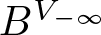 $B^{V_{-\infty}}$ agree (possibly up to permutation). These are integral linear conditions and hence exhibit $\mathcal M^{hor}_\Gamma(B \times \mathbb{R})_m^{\mathcal Z_{n,k}} \subset \mathcal M^{hor}_\Gamma(B \times \mathbb{R})_m$ as a finite union of integral affine subspaces, from which the result follows.
Remark 3.4. Denote by  $\mathcal Z_{n,k} = \cup_i Z_i$ the decomposition given by Proposition 3.3. Note that each $Z_i$ is given as (a linear subspace of) the image of evaluation maps $(ev_{-\infty},ev_{+\infty}):\mathcal M_\Gamma^{hor}(B\times\mathbb{R}) \to B^{n+m+k} \times B^{n+m+k}$. Therefore, in what follows, we will reduce statements about the $Z_i$ to the images of evaluation maps.
We now show that the (open subsets of) affine subspaces  $Z_i$ are isotropic for a suitable family of $p$-forms on $B^{2n} \times B^{2k}$. To simplify the notation, we will write $p_i : B^{2n} \times B^{2k} \to B$ for the composition of the permutation
 \begin{equation*}
(1,\dots,2n+2k) \mapsto (1,\dots,n,2n+1,\dots,2n+k,n+1,\dots,2n,2n+k+1,\dots,2n+2k)
\end{equation*}
\begin{equation*}
(1,\dots,2n+2k) \mapsto (1,\dots,n,2n+1,\dots,2n+k,n+1,\dots,2n,2n+k+1,\dots,2n+2k)
\end{equation*}with the projection onto the  $i$-th factor.
Proposition 3.5. Let  $0\neq \tilde\omega \in H^0(\wedge^p T^*_{\mathbb{Z}} B)$ be a non-zero tropical $p$-form. Then the $p$-form
 \begin{equation}
\omega=\sum_{i=1}^{n+k}p_i^*\tilde\omega - \sum_{i=n+k +1}^{2n+2k}p_i^*\tilde \omega \in H^0(\wedge^pT^*_{\mathbb{Z}}(B^{2n}\times B^{2k}))
\end{equation}
\begin{equation}
\omega=\sum_{i=1}^{n+k}p_i^*\tilde\omega - \sum_{i=n+k +1}^{2n+2k}p_i^*\tilde \omega \in H^0(\wedge^pT^*_{\mathbb{Z}}(B^{2n}\times B^{2k}))
\end{equation}vanishes on the  $Z_i$.
Proof. By Remark 3.4 it is enough to show that  $\omega$ vanishes on the image of the evaluation maps $(ev_{-\infty},ev_{+\infty}):\mathcal M_\Gamma^{hor}(B\times\mathbb{R}) \to B^{2n} \times B^{2k}$. Let then $h:\Gamma \to B\times \mathbb{R}$ be a parametrized tropical curve that is horizontal at infinity. Let $\eta: H^0(\mathcal T^*) \xrightarrow{\sim} H_1(\bar\Gamma,\partial\Gamma;\mathbb{R})$ be the isomorphism from Lemma 2.10. Denote by $\mathcal T^*_\infty \Gamma$ the direct sum of the stalks of $\mathcal T^*$ at the unbounded edges of $\Gamma$. Then we have a commutative square
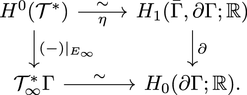
Recall from Section 2.3 that the isomorphism  $\eta:H^0(\mathcal T^*) \xrightarrow{\sim} H_1(\bar{\Gamma},\partial\Gamma;\mathbb{R})$ depends on a choice of orientation for the edges. For the purposes of this proof, we choose an orientation such that the unbounded edges—which are horizontal at infinity by Definition 2.16—agree with $\partial_t$, where $t$ is the coordinate of $\mathbb{R}$. Then, in the square above the map $\eta$ sends
 \begin{equation*}
(\alpha_e)\in \oplus_e T^*e \mapsto \sum_e \alpha_e(u_e)e \in H_1(\bar\Gamma,\partial\Gamma;\mathbb{R})
\end{equation*}
\begin{equation*}
(\alpha_e)\in \oplus_e T^*e \mapsto \sum_e \alpha_e(u_e)e \in H_1(\bar\Gamma,\partial\Gamma;\mathbb{R})
\end{equation*}(see Remark 2.11); the bottom horizontal map is the restriction
 \begin{equation*}
(\alpha_e)_{e\in E_\infty}\mapsto (\pm\alpha_e(\partial_t))_{e\in E_{\pm\infty}};
\end{equation*}
\begin{equation*}
(\alpha_e)_{e\in E_\infty}\mapsto (\pm\alpha_e(\partial_t))_{e\in E_{\pm\infty}};
\end{equation*}the left vertical map is the restriction to the stalks; and the right vertical map is the boundary operator of the long exact sequence of the pair 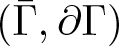 $(\bar\Gamma,\partial\Gamma)$, which sends a simplicial $1$-chain to its boundary. As before, we denote by $\mathcal D_\infty\Gamma \simeq \oplus_{e\in E_\infty}\mathcal D_e$ the direct sum of the stalks of $\mathcal D$ at the unbounded edges of $\Gamma$; note that $\mathcal D_\infty\Gamma \simeq TB^{2n + 2k}, 2n + 2k = |E_\infty|$. Then, using Lemma 2.15, we can extend the above square to a commutative diagram

where  $ev = ev_{(1,\dots,1,-1,\dots,-1)}$ maps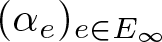 $(\alpha_e)_{e\in E_\infty}$ to $\sum_{e\in E_{\pm\infty}} \pm\alpha_e(\partial_t)$. Furthermore, for $v_i = (v_i^{1},\dots,v_i^{2n+2k}) \in T(B^{2n} \times B^{2k}), i = 1,\dots,p$, we have
 \begin{align*}
\omega(v_1\wedge\dots\wedge v_p)
&=
\sum_{i=1}^{2n}\tilde\omega(v^i_1\wedge\dots\wedge v_p^i) - \sum_{i=2n+1}^{2n+2k}\tilde\omega (v^i_1\wedge\dots\wedge v_p^i) \\
&=
\sum_{i=1}^{2n}\Phi_{\tilde\omega \wedge dt}(v^i_1\wedge\dots\wedge v_p^i)(\partial_t) + \sum_{i=2n+1}^{2n+2k}\Phi_{\tilde \omega \wedge dt}(v^i_1\wedge\dots\wedge v_p^i)(-\partial_t)\\
& = (ev\circ \Phi_{\tilde\omega\wedge dt})(v_1\wedge\dots\wedge v_p)
\end{align*}
\begin{align*}
\omega(v_1\wedge\dots\wedge v_p)
&=
\sum_{i=1}^{2n}\tilde\omega(v^i_1\wedge\dots\wedge v_p^i) - \sum_{i=2n+1}^{2n+2k}\tilde\omega (v^i_1\wedge\dots\wedge v_p^i) \\
&=
\sum_{i=1}^{2n}\Phi_{\tilde\omega \wedge dt}(v^i_1\wedge\dots\wedge v_p^i)(\partial_t) + \sum_{i=2n+1}^{2n+2k}\Phi_{\tilde \omega \wedge dt}(v^i_1\wedge\dots\wedge v_p^i)(-\partial_t)\\
& = (ev\circ \Phi_{\tilde\omega\wedge dt})(v_1\wedge\dots\wedge v_p)
\end{align*}where in the second equality we have used the identification 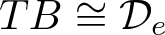 $TB \cong \mathcal D_e$ for any unbounded edge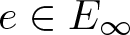 $e \in E_\infty$. The result now follows: if $v_1,\dots,v_p$ are tangent vectors to the image of an evaluation map
 \begin{equation*}
(ev_{-\infty},ev_\infty): \mathcal M_\Gamma^{hor}(B\times\mathbb{R}) \to B^{n+m+k} \times B^{n+m+k},
\end{equation*}
\begin{equation*}
(ev_{-\infty},ev_\infty): \mathcal M_\Gamma^{hor}(B\times\mathbb{R}) \to B^{n+m+k} \times B^{n+m+k},
\end{equation*}then there exist deformations 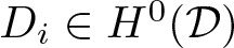 $D_i \in H^0(\mathcal D)$ such that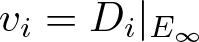 $v_i= D_i|_{E_\infty}$, and
 \begin{align*}
\omega(v_1\wedge\dots\wedge v_p)&=(ev \circ \Phi_{\omega\wedge dt})(D_1|_{E_\infty}\wedge \dots\wedge D_p|_{E_\infty})\\
&=(ev \circ \Phi_{\omega\wedge dt})(D_1\wedge\dots \wedge D_p)|_{E_\infty}\\
&= (\iota_*\circ\partial \circ \eta \circ \Phi_{\omega\wedge dt}) (D_1\wedge\dots \wedge D_p)\\
&=0.
\end{align*}
\begin{align*}
\omega(v_1\wedge\dots\wedge v_p)&=(ev \circ \Phi_{\omega\wedge dt})(D_1|_{E_\infty}\wedge \dots\wedge D_p|_{E_\infty})\\
&=(ev \circ \Phi_{\omega\wedge dt})(D_1\wedge\dots \wedge D_p)|_{E_\infty}\\
&= (\iota_*\circ\partial \circ \eta \circ \Phi_{\omega\wedge dt}) (D_1\wedge\dots \wedge D_p)\\
&=0.
\end{align*} Here we have used the commutativity of the top left square of Equation (12) in the second line, the commutativity of both the top right square and the bottom right triangle in the third line, and the fact that 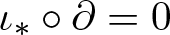 $\iota_*\circ\partial=0$ in the last line.
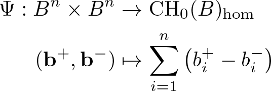
Recall from Definition 1.1 that we say  $\operatorname{CH}_0(B)_{hom}$ is infinite-dimensional if the maps
 \begin{equation}
\begin{split}
\Psi:B^n\times B^n &\to \operatorname{CH}_0(B)_{\hom}\\
(\mathbf{b}^+,\mathbf{b}^-) &\mapsto \sum_{i=1}^n \left( b_i^+ - b_i^-\right)
\end{split}
\end{equation}
\begin{equation}
\begin{split}
\Psi:B^n\times B^n &\to \operatorname{CH}_0(B)_{\hom}\\
(\mathbf{b}^+,\mathbf{b}^-) &\mapsto \sum_{i=1}^n \left( b_i^+ - b_i^-\right)
\end{split}
\end{equation}are not surjective for any  $n$. Proposition 3.5 together with the following Lemma will allow us to conclude that the existence of non-zero tropical $p$-forms, $p\geq 2$, implies infinite dimensionality of $\operatorname{CH}_0(B)_{\hom}$.
Lemma 3.6. ([Reference Roitman16, Lemma 9])
Let 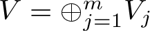 $V = \oplus_{j=1}^m V_j$ be a graded vector space and $0 \neq \omega_j \in \wedge^p V_j^*$ non-zero $p$-forms on $V_j$, $p \geq 2$. Denote by $pr_j: V \to V_j$ the natural projection. If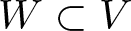 $W \subset V$ is an isotropic subspace for the $p$-form
 \begin{equation*}
\Omega = \sum_j pr^*_j \omega_j,
\end{equation*}
\begin{equation*}
\Omega = \sum_j pr^*_j \omega_j,
\end{equation*}then  $\dim W \leq \dim V - m$.
Theorem 3.7 If a tropical affine manifold  $B$ admits a non-zero tropical $p$-form for some $p \geq 2$, the group $\operatorname{CH}_0(B)_{\hom}$ is infinite-dimensional.
Proof. Let 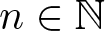 $n\in \mathbb{N}$ arbitrary; we will show the map $\Psi:B^n\times B^n \to \operatorname{CH}_0(B)_{\hom}$ of Equation (13) is not surjective. Note that $\Psi$ is surjective if and only if the projection
 \begin{equation*}
\mathcal Z_{n,k} \subset B^{2n} \times B^{2k} \to B^{2k}
\end{equation*}
\begin{equation*}
\mathcal Z_{n,k} \subset B^{2n} \times B^{2k} \to B^{2k}
\end{equation*}is surjective for all 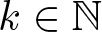 $k \in \mathbb{N}$. Let $0\neq \tilde \omega \in H^0(\wedge^p_{\mathbb{Z}} T^*B)$ be a non-zero tropical $p$-form and let $\omega$ be the form of Equation (11). It follows from Proposition 3.3 that $\mathcal Z_{n,k} = \cup_i Z_i$ decomposes as a countable union. Furthermore, each $Z_i$ is isotropic for $\omega$ by Proposition 3.5, thus
 \begin{equation*}
\dim Z_i \leq \dim (B^{2n}\times B^{2k}) - (2n + 2k)
\end{equation*}
\begin{equation*}
\dim Z_i \leq \dim (B^{2n}\times B^{2k}) - (2n + 2k)
\end{equation*}by Lemma 3.6. We have that  $\mathcal Z_{n,k} = \cup_i Z_i$ is a countable union of submanifolds of bounded dimension, hence the projection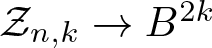 $\mathcal Z_{n,k} \to B^{2k}$ is surjective if and only if at least one of the restrictions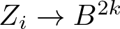 $Z_i \to B^{2k}$ is (the image of each $Z_i$ is an integral affine submanifold of $B^{2k}$, so if each such image is strictly lower dimensional, a countable union of them is also strictly lower dimensional). Now choose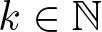 $k\in \mathbb{N}$ such that $\dim B^{2n} - 2n \lt 2k$, i.e. $\dim B^{2n} - 2n - 2k \lt 0$. Then we have
 \begin{align*}
\dim Z_i &\leq \dim (B^{2n}\times B^{2k}) - (2n + 2k) \\
& = \dim B^{2k} + (\dim B^{2n} - 2n - 2k)\\
& \lt \dim B^{2k}
\end{align*}
\begin{align*}
\dim Z_i &\leq \dim (B^{2n}\times B^{2k}) - (2n + 2k) \\
& = \dim B^{2k} + (\dim B^{2n} - 2n - 2k)\\
& \lt \dim B^{2k}
\end{align*}so the projection cannot be surjective.
3.2. Tropical Chow group of the Klein bottle
In this section, we consider a certain family of tropical Klein bottles and show that their Chow group of points are finite-dimensional. This shows that the existence of a non-zero tropical  $1$-form does not imply the tropical Chow group is infinite-dimensional.
Let  $\Gamma = \langle a,b |aba = b \rangle$ be the fundamental group of a Klein bottle, and consider the injection $\Gamma \hookrightarrow \operatorname{Aff}_{\mathbb{Z}} (\mathbb{R}^2)$ given by Equation (2). Let $K$ be the quotient
 \begin{equation*}
K := \mathbb{R}^2/\Gamma
\end{equation*}
\begin{equation*}
K := \mathbb{R}^2/\Gamma
\end{equation*}with the induced integral affine structure.
Proposition 3.8. The tropical Albanese map
 \begin{equation*}
\operatorname{alb}:\operatorname{CH}_0(K)_{\hom}\to \operatorname{Alb}(K)
\end{equation*}
\begin{equation*}
\operatorname{alb}:\operatorname{CH}_0(K)_{\hom}\to \operatorname{Alb}(K)
\end{equation*}is an isomorphism. In particular,  $\operatorname{CH}_0(K)_{\hom}$ is finite-dimensional.
Proof. Write  $p_1: K \to B_1$ (resp. $p_2: K \to B_2$) for the projection onto the first (resp. second) coordinate. Note that $B_1 = \mathbb{R}/(x\sim x+ x_0) \simeq S^{1}$ and
 \begin{equation*}
B_2 = \frac{\mathbb{R}}{y\sim y+ y_0,y \sim -y} \simeq [0,y_0/2].
\end{equation*}
\begin{equation*}
B_2 = \frac{\mathbb{R}}{y\sim y+ y_0,y \sim -y} \simeq [0,y_0/2].
\end{equation*}We will show that the tropical section
 \begin{align*}
s:B_1 \simeq S^{1} & \hookrightarrow K\\
\theta & \mapsto (\theta,0)
\end{align*}
\begin{align*}
s:B_1 \simeq S^{1} & \hookrightarrow K\\
\theta & \mapsto (\theta,0)
\end{align*}of  $p_1$ induces (by push forward) an isomorphism on $\operatorname{CH}_0$.
Since  $s$ is a section of $p_1$, the functoriality of Chow groups implies injectivity. To prove surjectivity, we first show that for any point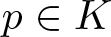 $p \in K$, one has
 \begin{equation*}
2(p - \iota(p)) \sim 0
\end{equation*}
\begin{equation*}
2(p - \iota(p)) \sim 0
\end{equation*}in  $\operatorname{CH}(K)$, where $\iota: K \to K$ is a reflection along the $x$-axis. Indeed,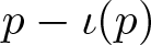 $p - \iota(p)$ lies in a fibre $F^2_y := p_2^{-1}(y) \simeq S^{1}$ of the projection $p_2$; note that $F^2_y$ is a tropical curve in $K$ (see the left part of Figure 5). It is easy to check that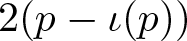 $2(p-\iota(p))$ is in the kernel of $\operatorname{CH}(F^2_y)_{\hom} \to \operatorname{Alb}(F^2_y)$, and since this map is an isomorphism by the tropical Abel theorem [Reference Mikhalkin and Zharkov13, Theorem 6.2] we conclude $2(p-\iota(p))\sim 0$ in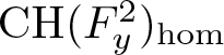 $\operatorname{CH}(F^2_y)_{\hom}$. Pushing forward this relation under the inclusion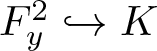 $F^2_y \hookrightarrow K$ one obtains the result.
Now let 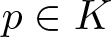 $p \in K$ be any point and denote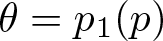 $\theta = p_1(p)$. We consider the homologically trivial $0$-cycle
 \begin{equation*}
4p - 4s(\theta) \sim 2p + 2\iota(p) - 4s(\theta),
\end{equation*}
\begin{equation*}
4p - 4s(\theta) \sim 2p + 2\iota(p) - 4s(\theta),
\end{equation*}where we have used the previous relation  $2(p - \iota(p))\sim 0$. By definition of $\iota$ one has that
 \begin{equation*}
p + \iota(p) - 2s(\theta) = (p - s(\theta)) - (s(\theta) - \iota(p))
\end{equation*}
\begin{equation*}
p + \iota(p) - 2s(\theta) = (p - s(\theta)) - (s(\theta) - \iota(p))
\end{equation*}Left: geometry of the relation  $2(p-\iota(p))\sim 0$. Right: geometry of the relation $4p - 4s(\theta) \sim 0$.
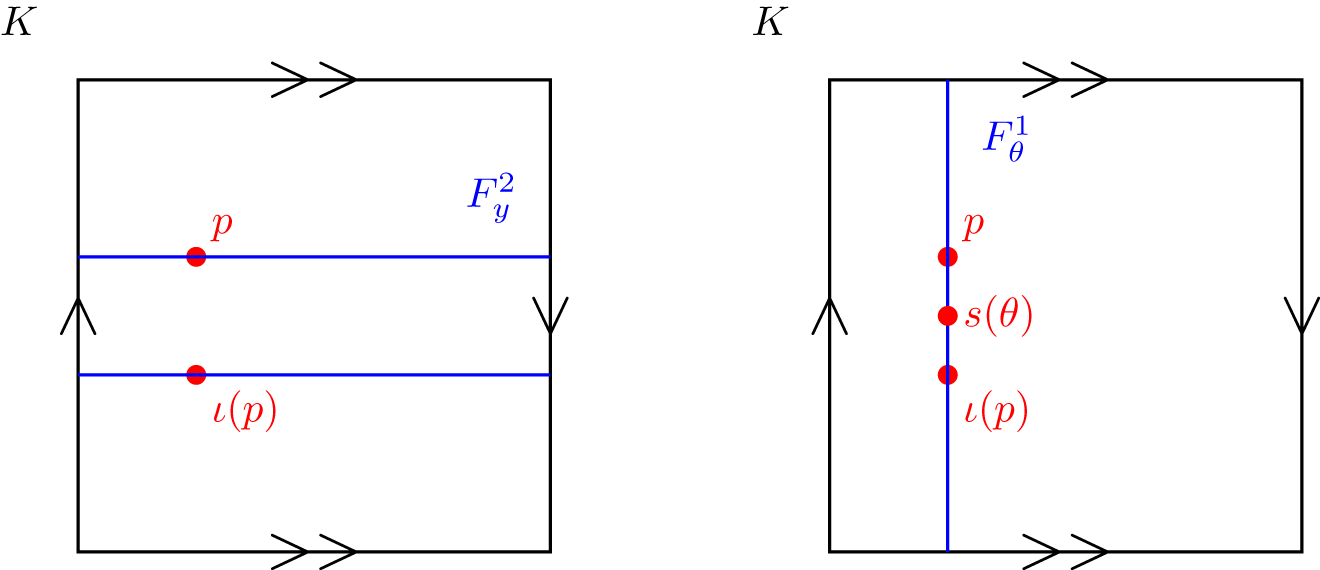
Figure 5 Long description
Long_Description: The image consists of two diagrams, each representing geometric relations within a space labeled K. The left diagram shows a rectangular shape with arrows indicating direction along the edges. Inside, two horizontal blue lines are drawn, labeled F superscript 2 subscript y at the top right. Two red points are marked on these lines, labeled p on the upper line and iota left parenthesis p right parenthesis on the lower line. The right diagram also features a rectangular shape with directional arrows along the edges. A vertical blue line is labeled F superscript 1 subscript theta at the top. Three red points are marked along this line, labeled p at the top, s left parenthesis theta right parenthesis in the middle and iota left parenthesis p right parenthesis at the bottom. Both diagrams illustrate the spatial arrangement and labeling of points within the geometric space K.
lies in the kernel of  $\operatorname{CH}_0(F^{1}_\theta)_{\hom} \to \operatorname{Alb}(F^{1}_\theta)$ (see right part of Figure 5), hence so does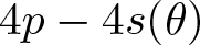 $4p - 4s(\theta)$. By the tropical Abel–Jacobi theorem,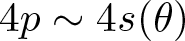 $4p \sim 4s(\theta)$ in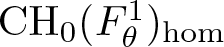 $\operatorname{CH}_0(F^{1}_\theta)_{\hom}$, and divisibility of $\operatorname{CH}_0(F^{1}_\theta)_{\hom} \simeq S^{1}$ further implies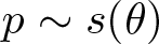 $p \sim s(\theta)$. Pushing forward this relation under the inclusion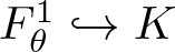 $F^{1}_\theta \hookrightarrow K$ yields the same result in $\operatorname{CH}_0(K)_{\hom}$, thus proving surjectivity.
Corollary 3.9. Let  $K$ be a tropical Klein bottle. Then $\operatorname{CH}_0(K)=\mathbb{Z}\oplus S^{1}$
Proof. Using the split short exact sequence
 \begin{equation*}
0 \to \operatorname{CH}_0(K)_{hom} \to \operatorname{CH}_0(K) \to \mathbb{Z} \to 0
\end{equation*}
\begin{equation*}
0 \to \operatorname{CH}_0(K)_{hom} \to \operatorname{CH}_0(K) \to \mathbb{Z} \to 0
\end{equation*}and Proposition 3.8, the statement of the Corollary is equivalent to  $\operatorname{Alb}(K)=S^{1}$. This is an immediate consequence of $H^0(T_{\mathbb{Z}}^* K)=\mathbb{Z}$, generated by the invariant covector of the monodromy.
Acknowledgements
I would like to thank my advisor, Nick Sheridan, for his constant support and guidance. I am grateful to Jeff Hicks for reading and commenting on an earlier draft of this paper, as well as pointing out that one can recover Mumford and Roitman’s result when there is a tropicalization. I also thank Arend Bayer for suggesting to try to find a tropical analogue of Mumford’s theorem, which led to the results in this paper. This work was supported by an ERC Starting Grant (award number 850713-HMS).


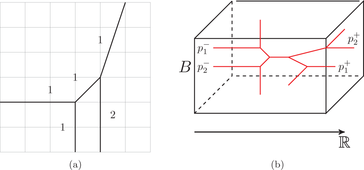


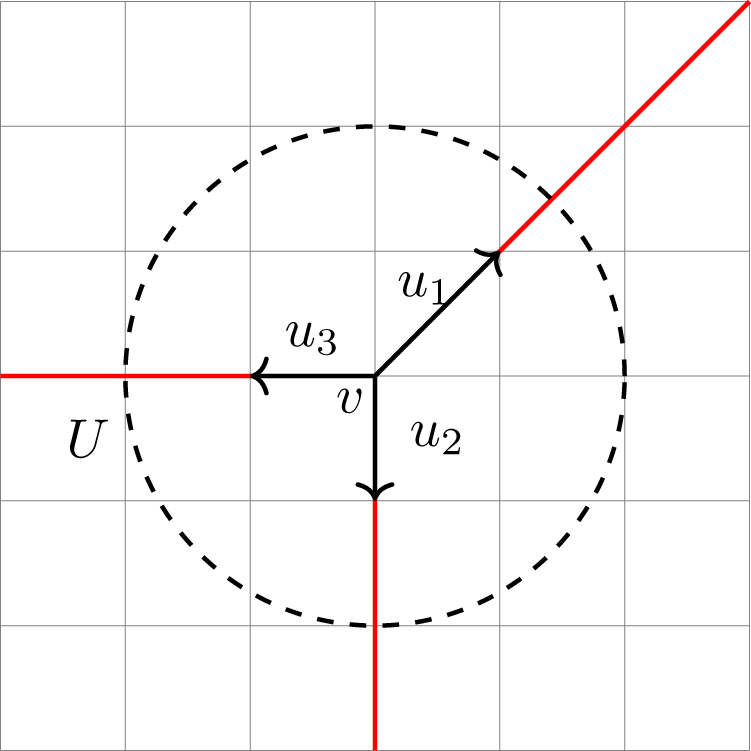
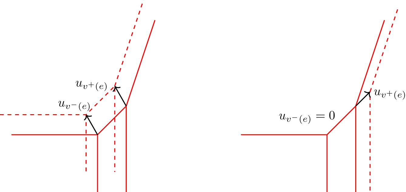


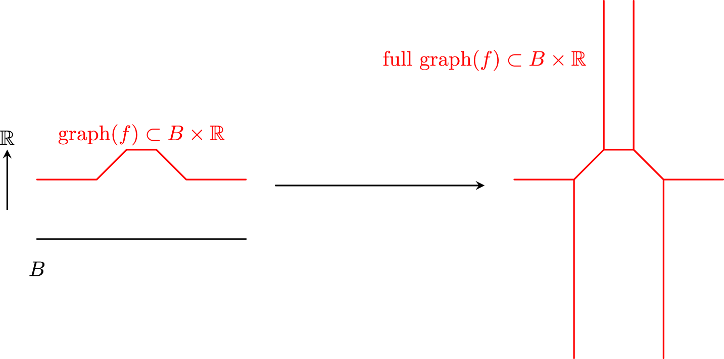


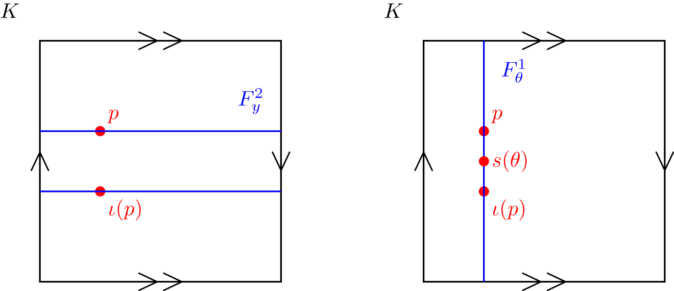


 Open access

