


1. INTRODUCTION
Partitioning Earth's climate history into internal variability and forced change is crucial for our understanding of climate dynamics. Although the definitional lines are somewhat blurred, internal climate variability is that which occurs in the absence of any changes to the external forcing of the climate system. External forcing is generally taken to be changes in atmospheric composition, insolation, or continental geometry, and volcanic eruptions. Internal climate variability sets the irreducible lower bound on the predictability of future climate: the particular climate trajectory that we will ride into the future depends both on the changes in external forcing and also on the internal variability which, analogous to a weather forecast, depends unknowably on the details of the current state of the system (e.g. Hawkins and Sutton, Reference Hawkins and Sutton2009; Deserand others, Reference Deser, Phillips, Bourdette and Teng2012).
For timescales beyond the instrumental record, we must rely on paleoclimate proxies to reconstruct the histories of both internal climate variability and climate change. Arguably the most important paleoclimate research in recent decades was the demonstration that the magnitude of the change in global-mean temperature in the past century exceeds the range of variability in the late Holocene (e.g. Mann and others, Reference Mann, Bradley and Hughes1998). This was a critical contribution to the formal identification of an anthropogenic climate-change ‘signal’ above the climate-variability ‘noise’. However, the fact that both climate change and climate variability are wrapped up in the same paleoclimate records can complicate their interpretation. The distinction between climate change and climate variability is vital to keep clear, because the former challenges us to identify and quantify the forcing agents, whereas the latter represents the business-as-usual operation of the system and requires no further explanation.
Glacial valleys are important repositories of paleoclimate information. In many places, reconstructions of glacier history provide the primary narrative of regional climate history, against which other proxy records are evaluated. In the past fifteen years, a series of studies has sought to characterize the response of glaciers to climate variability (Oerlemans, Reference Oerlemans2000, Reference Oerlemans2001; Reichert and others, Reference Reichert, Bengtsson and Oerlemans2002; Huybers and Roe, Reference Huybers and Roe2009; Roe and O'Neal Reference Roe and O'Neal2009; Roe, Reference Roe2011; Roe and Baker, Reference Roe and Baker2014; Anderson and others, Reference Anderson, Roe and Anderson2014; Rowan and others, Reference Rowan2014). Here the relevant climate variable is mass balance. After detrending, observations of glacier mass balance cannot generally be distinguished from a normally distributed, white-noise time series (e.g. Burke and Roe, Reference Burke and Roe2014; Medwedeff and Roe, Reference Medwedeff and Roe2016). A white-noise time series has uniform power at all frequencies in its spectrum, and has zero persistence in its time series (i.e. fluctuations at different times are uncorrelated; Box and others, Reference Box, Jenkins and Reinsel2008). Because glaciers act as low-pass climate filters, a glacier will generate a reddened response (more power at low frequencies) and so undergo long, persistent fluctuations even when the climate itself has no persistence. The above-mentioned studies modeled the glacier response to white-noise mass-balance forcing and found standard deviations in length (≡ σ
L) varying from a few hundred meters up to a kilometer, depending on glacier geometry, climatic setting and model details. Glaciers typically have response times of up to a few decades (e.g. Leclercq and Oerlemans, Reference Leclercq and Oerlemans2012). By definition of the standard deviation, a glacier will spend ${\rm \sim} 5\% $
of its time outside ± 2σ
L (i.e., maxima and minima are at least 4σ
L apart). Therefore these studies establish that century-scale, kilometer-scale fluctuations in glacier length will occur in response to a climate that has no persistence, but consists only of the observed year-to-year variability due to the vagaries of the weather. This then sets the null hypothesis, against which past glacier length fluctuations should be evaluated statistically, to determine if they, in fact, indicate a climate change.
${\rm \sim} 5\% $
of its time outside ± 2σ
L (i.e., maxima and minima are at least 4σ
L apart). Therefore these studies establish that century-scale, kilometer-scale fluctuations in glacier length will occur in response to a climate that has no persistence, but consists only of the observed year-to-year variability due to the vagaries of the weather. This then sets the null hypothesis, against which past glacier length fluctuations should be evaluated statistically, to determine if they, in fact, indicate a climate change.
In this study we follow a line of research pioneered by Reichert and others (Reference Reichert, Bengtsson and Oerlemans2002). While glacier mass-balance observations are generally consistent with white noise, other data indicate that this may be due to the limited duration of mass-balance records. Long instrumental records of some other meteorological fields (temperature and, to a lesser degree precipitation), proxy paleoclimate records, and theoretical and numerical climate models all suggest that there is a degree of persistence in internal climate variability. In this study we use a numerical flowline model, together with a newly developed analytical glacier model, to show that adding even a small amount of persistence, so small that it is hard to detect in long instrumental records, substantially enhances glacier length fluctuations compared with a climate without persistence. In turn, this has a big impact on the excursion probabilities. Since the degree of persistence that pertains to glacier mass balance is difficult to establish from observations, the results imply greater uncertainty than has typically been recognized in the magnitude of the glacier response to internal climate variability. This makes it harder to identify true climate change in the glacier record.
2. TWO MODELS OF CLIMATIC PERSISTENCE
We consider two commonly invoked statistical models of climatic persistence. The first is a first-order autoregressive process (≡ AR(1); e.g. Box and others, Reference Box, Jenkins and Reinsel2008). Let b t be the annual-mean mass balance in year t. An AR(1) process can be written as
 $${b_t} = r{b_{t - \Delta t}} + {a_0}\Delta t\hskip1pt{\mu _t},$$
where Δt = 1a, r and a 0 are constants and μ t is a random number drawn from a normally-distributed stochastic process. Thus b t depends in part on its value in the previous year (and so has persistence), and in part on a random stochastic impulse occurring in the current year. r is the autocorrelation coefficient at lag 1 a. Equation (1) is the discrete form of the continuous equation: db/dt + b/τ c = a 0 μ(t), and so r can be related to a climatic persistence timescale (or memory), τ c: r = 1 − Δt/τ c. This model of persistence was introduced into climate science in a series of papers by Klaus Hasselmann and colleagues (e.g. Hasselmann, Reference Hasselmann1976; Frankignoul and Hasselmann, Reference Frankignoul and Hasselmann1977), which demonstrated that persistence in sea-surface temperatures was the result of the ocean-mixed layer acting to integrate rapid and essentially random, uncorrelated fluctuations of air-sea heat fluxes.
Note that one can also consider a higher-order autoregressive process, AR(p), which depends on the previous p states (e.g. Box and others, Reference Box, Jenkins and Reinsel2008), and which can be interpreted as the discrete form of a p th-order ordinary differential equation. Reichert and others (Reference Reichert, Bengtsson and Oerlemans2002) fit an AR(3) process to climate-model output for Nigardsbreen Glacier in Norway, for instance. The AR(3) coefficients they fit imply a persistence timescale of 1.5 a, and also an underlying damped oscillation with a 3 a period and a 1 a phase-memory. It is important to make a physical interpretation of the higher-order AR(p) process, and to establish the statistical necessity of the higher-order model via standard methods (e.g. Box and others, Reference Box, Jenkins and Reinsel2008). We only consider AR(1) here.
For an AR(1) process, the power spectral density as a function of frequency and lag-1 a autocorrelation (≡ P b(f, r)), is given by:
 $${P_{\rm b}}(\,f,r) = \displaystyle{{{P_0}} \over {1 + {r^2} - 2r\cos (2\pi \Delta tf)}},\quad {\rm on}\quad 0 \le f \le \displaystyle{1 \over {2\Delta t}}.$$
where P 0 is a constant, defined in the Appendix. P b(f, r) increases towards lower frequencies, and by analogy with spectra for visible light, is often termed red noise.
The autocorrelation function (ACF) is the formal statistical description of the structure of the persistence in a time series (e.g. Box and others, Reference Box, Jenkins and Reinsel2008), and it characterizes the similarity between the data as a function of the time lag between them. Let nΔt represent a lag of n years. The ACF is defined by ρ(nΔt) = 〈b
t
b
t−nΔt
〉. From the Wiener-Kinchin theorem, the ACF is the Fourier transform of the power spectrum: $\rho (n\Delta t) = {{\int_0^{{f_0}} {P_{\rm b}}(f)\cos (2\pi n\Delta tf){\rm d}f} / {\int_0^{{f_0}} {P_{\rm b}}(f){\rm d}f}}$
.
$\rho (n\Delta t) = {{\int_0^{{f_0}} {P_{\rm b}}(f)\cos (2\pi n\Delta tf){\rm d}f} / {\int_0^{{f_0}} {P_{\rm b}}(f){\rm d}f}}$
.
For an AR(1) process the ACF is:
 $$\rho (n\Delta t) = {\left( {1 - \displaystyle{{\Delta t} \over {{\tau _{\rm c}}}}} \right)^n}{\rm \simeq} \exp \left( { - \displaystyle{{n\Delta t} \over {{\tau _{\rm c}}}}} \right),$$
and thus ρ asymptotes exponentially towards zero with an e-folding timescale, τ c.
The second model for persistence characterizes the spectrum of a time series as a power law. This form is suggested by several analyses of long instrumental and paleoclimate proxy records for temperature (e.g. Pelletier, Reference Pelletier1997, Reference Pelletier1998; Fraedrich and Blender, Reference Fraedrich and Blender2003; Fraedrich and others, Reference Fraedrich, Luksch and Blender2004; Huybers and Curry, Reference Huybers and Curry2006), and also for precipitation and other hydrological variables (Hurst, Reference Hurst1951; Ault and others, Reference Ault2013). Let ν be the slope of the power spectrum when plotted on logarithmic axes. So in this case, the spectrum P b(f, ν), is defined by:
 $${P_{\rm b}}(\,f,\nu ) = {P_0}{({\,f_0}/f)^\nu}, $$
where P 0 is the spectral density at frequency f 0 = 1/(2Δt), the maximum resolvable frequency from an annual-mean time series; and ν is a positive constant. Thus, spectral power continually increases towards low frequencies.
For the ACF there is an exact analytical solution in the form of an ordinary hypergeometric function.
 $$\rho (n\Delta t{) =\; _2}{F_1}\left[ {\displaystyle{{1 - \nu} \over 2},\left\{ {\displaystyle{1 \over 2},\displaystyle{{3 - \nu} \over 2}} \right\}, - {{(2\pi n\Delta t{\,f_0})}^2}} \right],$$
which looks intimidating but the key point is that, at large lags, it decays towards zero as (nΔt) ν−1 (e.g. Percival and others, Reference Percival, Overland and Mofjeld2001; Box and others, Reference Box, Jenkins and Reinsel2008). It thus decays much more slowly than an AR(1) process (Eqn 3), and so exhibits greater persistence at long timescales. For this reason Eqn (4) is referred to as a ‘long memory’ process. This behavior will be shown in Figure 2.
Huybers and Curry (Reference Huybers and Curry2006) present spatial maps of ν for 100 year-long temperature observations, and find values between 0 and 0.5 over land, with the highest values confined to maritime climate settings. Values can exceed 1 over the ocean, particularly in the tropics. Ault and others (Reference Ault2013) fit Eqn (4) to spectra of observed precipitation in western North America and find a patchwork pattern with ν ranging from ~−0.2 to +0.5, but with marginal statistical significance. Persistence evaluated from paleoclimate proxy time series should be regarded with some caution, since many of the proxies themselves act as integrators of climate, which together with dating uncertainty and post-depositional processes can act to redden the proxy time series independent of the driving climate. But such datasets do indicate that internal variability can be characterized as a power-law spectrum (Pelletier, Reference Pelletier1997, Reference Pelletier1998; Fraedrich and Blender, Reference Fraedrich and Blender2003; Fraedrich and others, Reference Fraedrich, Luksch and Blender2004; Huybers and Curry, Reference Huybers and Curry2006). Furthermore there are theoretical grounds to think that power-law behavior should be expected across decadal to millennial frequencies: for quasi-diffusive heat uptake in the deep ocean, progressively more of the ocean becomes involved at low frequencies, increasing the effective inertia of the climate system (Hoffert and others, Reference Hoffert, Callegari and Hsieh1980; Pelletier, Reference Pelletier1997; Fraedrich and others, Reference Fraedrich, Luksch and Blender2004), which is also diagnosed in comprehensive climate models (e.g. Zhu and others, Reference Zhu, Fraedrich, Liu and Blender2010; MacMynowski and others, Reference MacMynowski, Shin and Caldeira2011). Power-law spectra can also be generated by a fractionally differenced process, which is equivalent to an aggregation of AR(1) processes with many different timescales (Beran, Reference Beran1994; Percival and others, Reference Percival, Overland and Mofjeld2001; Box and others, Reference Box, Jenkins and Reinsel2008).
2.1. Observed variability and persistence in glacier mass-balance records
We first evaluate the variability and persistence of three of the longest annual-mean mass-balance observations available. Our goal is not to present a comprehensive evaluation of glacier mass-balance records, which is done in Medwedeff and Roe (Reference Medwedeff and Roe2016), but the results shown here are typical. The longest continuous mass-balance record is that on Clariden glacier, Switzerland (since 1914), although the measurements are only at two snow stakes, and so not necessarily representative over the whole glacier; Storbreen (since 1949) is the longest record in Norway; and South Cascade glacier in Washington State (since 1959) is the longest in North America.
Figure 1a presents these records after they have been linearly detrended to remove any anthropogenic trend. The standard deviations in mass balance (≡ σ b) and 95% bounds for each glacier are: Clariden, 0.74 {0.65, 0.86} m a−1; Storbreen, 0.69 {0.58, 0.83} m a−1; South Cascade, 1.04 {0.87, 1.3} m a−1, where the confidence bounds have been calculated assuming the n-years sample variance follows a χ 2 distribution with n − 1 degrees of freedom (e.g. VonStorch and Zwiers, Reference vonStorch and Zwiers1999). All three datasets are consistent with a normal distribution at better than 95% confidence based on a Jarque-Bera test (e.g. Steinskog and others, Reference Steinskog, Tjøtheim and Kvamstø2007).
Three long records of observed annual-mean glacier mass balance. Clariden (upper stake), Switzerland (95 a, σ
b = 0.74 m a−1); Storbreen, Norway (63 a, σ
b = 0.69 m a−1); and South Cascade, USA (54 a, σ
b = 1.04 m a−1). (a) Time series of the observations, with the linear trend and mean removed. (b) Autocorrelation function. The horizontal dashed lines are drawn at $2/\sqrt n $
, where n is the length of each record in years – these lines indicate the level above which the lag 1 a autocorrelation should lie to reject the null hypothesis of white noise at better than 95% confidence (Bartlett, Reference Bartlett1946; Box and others, Reference Box, Jenkins and Reinsel2008). (c) Power spectra (unwindowed periodogram) of mass-balance data. Dashed lines show the best-fit slopes (based on a least-squares linear regression). All slopes are positive, but none are significantly different from zero at better than 95% confidence.
$2/\sqrt n $
, where n is the length of each record in years – these lines indicate the level above which the lag 1 a autocorrelation should lie to reject the null hypothesis of white noise at better than 95% confidence (Bartlett, Reference Bartlett1946; Box and others, Reference Box, Jenkins and Reinsel2008). (c) Power spectra (unwindowed periodogram) of mass-balance data. Dashed lines show the best-fit slopes (based on a least-squares linear regression). All slopes are positive, but none are significantly different from zero at better than 95% confidence.

Most mass-balance records are not as long as those we selected, of course, and it is important to emphasize that, for shorter records, the uncertainty estimates on σ b are quite large. For a 20 a mass-balance record, for instance, the 95% bounds are {0.76, 1.46} times the standard deviation of the data sample. In other words, for many records, there is approximately a factor of two uncertainty in σ b (Medwedeff and Roe, Reference Medwedeff and Roe2016).
Figure 1b shows the ACFs for the three records. The null hypothesis of no persistence can only be rejected at 95% confidence if the lag one-year autocorrelation exceeds $2/\sqrt n $
(Bartlett, Reference Bartlett1946; Box and others, Reference Box, Jenkins and Reinsel2008). As is clear from Figure 1, on the basis of this test one concludes that all three records cannot be distinguished from a null hypothesis that the fluctuations are uncorrelated (i.e. they are white noise). This is confirmed using standard algorithms for selecting and fitting AR(p) models (e.g. Box and others, Reference Box, Jenkins and Reinsel2008), which identify AR(0) as the best description for all three records. Burke and Roe (Reference Burke and Roe2014) fit AR(p) models to long instrumental records and glacier mass-balance records in Europe, and also concluded persistence could not be definitively established.
$2/\sqrt n $
(Bartlett, Reference Bartlett1946; Box and others, Reference Box, Jenkins and Reinsel2008). As is clear from Figure 1, on the basis of this test one concludes that all three records cannot be distinguished from a null hypothesis that the fluctuations are uncorrelated (i.e. they are white noise). This is confirmed using standard algorithms for selecting and fitting AR(p) models (e.g. Box and others, Reference Box, Jenkins and Reinsel2008), which identify AR(0) as the best description for all three records. Burke and Roe (Reference Burke and Roe2014) fit AR(p) models to long instrumental records and glacier mass-balance records in Europe, and also concluded persistence could not be definitively established.
An alternative measure of persistence is to evaluate whether the power spectra of the records have non-zero slopes. Figure 1c shows the power spectra for the three records (unwindowed periodograms), together with the best-fit slopes, based on a least-squares linear regression. The results for the slopes, ν, are: Clariden, 0.25 ± 0.32 (2σ); Storbreen, 0.23 ± 0.61 (2σ); South Cascade, 0.09 ± 0.64 (2σ). For all the records the slopes are positive, but the 2σ ranges all straddle zero and so none are statistically different from ν = 0 (Clariden gets close with a p value of 0.12). Therefore, by this measure also, one concludes the observations cannot be distinguished from white noise.
Medwedeff and Roe (Reference Medwedeff and Roe2016) evaluate the full, global mass-balance dataset available from the World Glacier Monitoring Service (WGMS, Reference Zemp2013 and earlier issues) and find these results apply more broadly: observed annual-mean and season-mean mass-balance records are consistent with white noise (plus a linear trend).
We are therefore left with the situation that, while paleoclimate proxies and long instrumental records both suggest that there is a degree of persistence in climate time series (which varies as a function of location and climate variable), glacier mass-balance records are too short to detect such persistence statistically, or to accurately determine its type (i.e. AR(1) or power law) or degree (e.g. Percival and others, Reference Percival, Overland and Mofjeld2001). Nor can persistence in mass balance be easily inferred from other climate variables. Persistence is different for different variables. Glacier mass balance reflects a complex amalgam of many variables, and also depends in part on other stochastic processes such as avalanching and drifting. Nonetheless, as has been preliminarily explored by Reichert and others (Reference Reichert, Bengtsson and Oerlemans2002), climatic persistence has the potential to significantly enhance glacier length fluctuations. In this paper we take a what-if approach: what if climatic persistence, of a degree that is hard to detect, exists in glacier mass balance? What would be the impact of such persistence on the amplitude of glacier length fluctuations? The implications for the interpretation of past glacier records are broached in Section 4.
2.2. Synthetic climate time series with persistence
To explore the impacts of possible undetected persistence in mass balance on the interpretation of glacier-length records, we first generate synthetic mass-balance records with differing degrees of persistence. We then compare the theoretical glacier responses to these synthetic mass-balance histories with the responses that would be predicted under the erroneous assumption that the mass-balance fluctuations represent white noise.
We generate five synthetic 10 ka mass-balance time series using the method outlined by Percival and others (Reference Percival, Overland and Mofjeld2001). For a given choice of r or ν, the time series is generated from the Fourier transform of the spectrum amplitude (the square root of either Eqn (2) or (4)), multiplied by a random phase at each frequency. We use the same set of random phases for each time series, to facilitate comparison.
Our control mass-balance time series is white noise, with standard deviation σ b = 1 m a−1. For power-law persistence, we take values for ν of 0.25 and 0.4, since these sit within the range suggested for land-based climate variables. The lag one-year autocorrelation coefficients for such power-law persistence are 0.17 and 0.28 (Eqn 5), and these are the two values we use for r for AR(1)-type persistence. The memory, τ c, associated with these r values is 1.2 and 1.4 a, respectively. Based on the ~95% confidence intervals (Bartlett, Reference Bartlett1946), for a given r it takes n ~ (2/r)2 years to detect persistence. Thus, for our choices for ν of 0.25 and 0.4 it would require ~150 and 50 a of data, respectively, before persistence could be established. Such durations are comparable with some of the longest available instrumental and glacier mass-balance records. In other words we are emulating a realistic situation: we are introducing persistence with a magnitude that is hard to detect in observations.
The inclusion of persistence enhances the variance of a time series. However if the presence of persistence went undetected, the measured standard deviation would be taken to be the standard deviation of a white-noise process. The parameters of the assumed white noise used to predict glacier length fluctuations would then be based on this standard deviation. We therefore apply a correction, normalizing each time series so the standard deviation is equal to that of the control series (σ b = 1 m a−1). This ensures that the variance we use to drive the glacier models is consistent with what would be determined from observations – the only thing that is different is the persistence present in each time series. This correction is conservative in the sense that it reduces the resulting glacier variance. Without the correction, adding persistence would increase the standard deviation of mass balance (and glacier response) by 1.5, 4.2, 15 and 29%, for r = 0.17, 0.28, ν = 0.25, 0.4 respectively.
Figure 2a presents a 100 a segment of each of these synthetic climate time series. The series are virtually indistinguishable by eye, but the ACFs (Fig. 2b) reveal the differences. The AR(1) processes asymptote exponentially to zero (Eqn 3), whereas the ACFs of the power-law processes decline more slowly (Eqn 5) and thus represent a climate with a small-but-persistent chance that a series of successive years have the same sign anomaly (i.e. a long memory). The spectra are shown in Figure 2c and show that the synthetic time series accurately match the theoretical power spectra.
Synthetic mass-balance records, with differing degrees of persistence. (a) a 100 a time slice from the 10 ka realizations used to drive the glacier models. Time series for white noise, ν = 0.25, 0.40 and r = 0.17, 0.28 are shown, and have been normalized so that σ b = 1.0 m a−1 in each case. For clarity, the time series have been successively offset by 2000 mm on the y-axis. (b) Autocorrelation function for the five time series, indicating the persistence present in each record. (c) Power spectra (windowed periodogram) of the five time series (thick curves), and the theoretical spectra for each process (thin curves, see Eqns (2) and (4)). The discrepancies at the lowest frequencies are artifacts of the windowing.

In Section 3, we drive two different glacier models with these synthetic mass-balance time series. We also derive algebraic formulae that capture the impact of climatic persistence on glacier length.
3. IMPACT OF CLIMATIC PERSISTENCE ON GLACIER LENGTH
The first glacier model we use is the numerical flowline model from Roe and O'Neal (Reference Roe and O'Neal2009), with shallow-ice dynamics and basal sliding. It uses the same set of parameters as Roe and Baker (Reference Roe and Baker2014), characteristic of the small Alpine glaciers around Mt. Baker in Washington State, U.S.A. Readers are referred to Roe and Baker (Reference Roe and Baker2014) for the equations and more details.
The second model is the three-stage model, also of Roe and Baker (Reference Roe and Baker2014), a linear model for length fluctuations around a prescribed mean state, which was shown to closely emulate the behavior of the numerical model under a wide range of parameter choices. Its relatively simple form makes it an extremely versatile tool. It provides analytic solutions for important metrics of the response, such as a glacier's power spectrum, ACF, variance and excursion probabilities in response to climate variability, and a glacier's sensitivity to climate trends and step-changes. The three-stage equation is
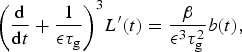 $${\left( {\displaystyle{{\rm d} \over {{\rm d}t}} + \displaystyle{1 \over {{\epsilon} {\tau _{\rm g}}}}} \right)^3}L^{\prime}(t) = \displaystyle{\beta \over {{{\epsilon} ^3}\tau _{\rm g}^2}} b(t),$$
where L′ is the perturbation in length away from a prescribed mean state; τ
g = −H/b
term
is the glacier response timescale originally proposed by Jòhannesson and others (Reference Jòhannesson, Raymond and Waddington1989), where H is the mean thickness, and b
term
is the (negative) net mass balance at the glacier terminus, both in the mean state; and ε is a constant ( $ = 1/\sqrt 3 {\rm \simeq} 0.58$
). The glacier geometry also determines β = A
tot
/(wH), where A
tot
is the total glacier area and w is the characteristic valley width at the terminus. As in Roe and Baker (Reference Roe and Baker2014), for our standard control glacier, we take τ
g = 6.74a, and β = 178 (unitless).
$ = 1/\sqrt 3 {\rm \simeq} 0.58$
). The glacier geometry also determines β = A
tot
/(wH), where A
tot
is the total glacier area and w is the characteristic valley width at the terminus. As in Roe and Baker (Reference Roe and Baker2014), for our standard control glacier, we take τ
g = 6.74a, and β = 178 (unitless).
Equation (6) reflects the three stages of glacier adjustment identified and described in Roe and Baker (Reference Roe and Baker2014): changes in mass balance first cause changes in thickness, which then causes changes in ice flux at the terminus, which finally causes changes in length. These three stages are robust to the spatial pattern of mass-balance changes, and are intrinsic to the high-frequency response of a glacier. Roe and Baker (Reference Roe and Baker2014) further showed that Eqn (6) could also be written as a discrete equation in time steps of Δt = 1a. The discrete equation more closely matches the nature of actual mass balance, coming as it does in discrete winter and summer seasons. Roe and Baker (Reference Roe and Baker2014) showed that, for white-noise forcing, the length variance ( $ = \sigma _{\rm L}^2 $
) for the discrete three-stage model is:
$ = \sigma _{\rm L}^2 $
) for the discrete three-stage model is:
 $$\sigma _{\rm L}^2 = {\beta ^2}\tau _{\rm g}^2 {\sigma _{\rm b}^2} \displaystyle{{(1 - \kappa )(1 + 4{\kappa ^2} + {\kappa ^4})} \over {2\Delta t{{(1 + \kappa )}^5}}},$$
where κ = (1 − (Δt/ετ g)). In the limit as ετ g ≫ Δt this simplifies to:
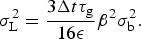 $$\sigma _{\rm L}^2 = \displaystyle{{3\Delta t{\tau _{\rm g}}} \over {16{\epsilon}}} {\beta ^2}{\sigma _{\rm b}^2}. $$
For σ b = 1 m a−1, Eqn (7) predicts σ L = 284 m, which agrees closely with the output from numerical flowline model, σ L = 285 m. The time series of length fluctuations from the numerical model and the three-stage model are essentially identical (grey and black lines in Fig. 3), confirming that the three-stage model emulates ice-flow dynamics very effectively.
Glacier length fluctuations driven by climates with differing persistence. (a) 2 ka time slices of glacier-length anomalies for the five climate time series. The thick curves are the output from the numerical flowline model, the thin curves are calculated from the linear three-stage model of Roe and Baker (Reference Roe and Baker2014). For clarity, the time series have been successively offset by 1000 m. The greater variance for persistent climates is evident by eye. (b) The autocorrelation function of the glacier response. Note the expanded x-axis scale compared with Figure 2, and that the white noise and AR1 curves plot nearly on top of each other. (c) Power spectra of glacier response (windowed periodogram). Thick curves are from the numerical flowline model, thin curves are the theoretical curves from the three-stage model of Roe and Baker (Reference Roe and Baker2014).

Let R be the ratio of the glacier variance with-and-without persistence in mass-balance forcing. In the Appendix we derive expressions from the three-stage model. For persistence based on an AR(1) process, we find:
 $${R_r} \equiv \displaystyle{{{{\left. {{\sigma _{\rm L}^2}} \right \vert} _r}} \over {{{\left. {{\sigma _{\rm L}^2}} \right \vert} _{r = 0}}}} = \displaystyle{{(1 - {r^2})} \over {{{(1 - r)}^2}}} \cdot \displaystyle{{{\epsilon} {\tau _{\rm g}}(3{{\epsilon} ^2}\tau _{\rm g}^2 + 9{\epsilon} {\tau _{\rm g}}{\tau _{\rm c}} + 8\tau _{\rm c}^2 )} \over {3({\epsilon} {\tau _{\rm g}} + {\tau _{\rm c}}{)^3}}}.$$
In the limit of ετ g ≫ τ c, this simplifies to:
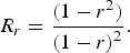 $${R_r} = \displaystyle{{(1 - {r^2})} \over {{{(1 - r)}^2}}}.$$
For persistence based on a power-law process, we find:
 $${R_\nu} \equiv \displaystyle{{{{\left. {\sigma _{\rm L}^2} \right \vert} _\nu}} \over {{{\left. {\sigma _{\rm L}^2} \right \vert} _{\nu = 0}}}} = \displaystyle{{{\pi ^\nu} {{({\epsilon} {\tau _{\rm g}}/\Delta t)}^\nu} (1 - {\nu ^2})(\nu + 3)\sec (\nu \pi /2)} \over 3}.$$
These expressions can be used to calculate the standard deviation of glacier length:
 $${\sigma _{\rm L}}{ \vert _{r,\nu}} = \sqrt {{R_{r,\nu}}} \cdot {\sigma _{\rm L}}{ \vert _{wn}},$$
where σ L| wn is the response to white-noise forcing Eqn (7) or (8). Equations (9) and (11) allow for efficient computation across a wide range of parameters.
For the mass-balance time series generated by AR(1) processes with r = 0.17 and 0.28, the numerical flowline model responds with σ L = 336 and 377 m, respectively. These are increases of 18 and 32% over σ L for white-noise forcing, and Eqn (9) gives good agreement, predicting 17 and 31%, respectively. The length time series for numerical and three-stage models are shown in Figure 3a, and the increased length variability for increasing r can be seen by eye, particularly if you focus on adjacent maxima and minima. Furthermore, we see that the three-stage model emulates the numerical flowline model very well. The ACFs (Fig. 3b) look very similar to the white-noise case, but the spectra show the enhanced power at low frequencies (Fig. 3c). At frequencies <1/100 a−1, the glacier dynamics no longer damp the response, and the glacier exists in near-equilibrium with the climate forcing (e.g. Roe and Baker, Reference Roe and Baker2014).
For the mass-balance time series generated by power-law processes with ν = 0.25 and 0.4, the numerical flowline model responds with σ L = 399 and 489 m, respectively. These are increases of 40 and 72% over σ L for white-noise forcing, and Eqn (11) gives good agreement, predicting 43 and 79%, respectively. Again the increase in variance is clear by eye in the time series in Figure 3a, with the three-stage model again accurately reproducing the behavior of the numerical flowline model. In contrast with the AR(1) case, the ACFs for the power-law climate (Fig. 3b), clearly show the extra persistence at large lags. These ACFs and the larger increase in variance are consistent with the spectra (Fig. 3c) that show power continuing to increase towards lower frequencies.
Reichert and others (Reference Reichert, Bengtsson and Oerlemans2002) fit an AR(3) process to a climate-model simulation of mass balance for Nigardsbreen, Norway, and generated an increase in σ L of 36%. However our results are hard to directly compare because of the different AR(p) models, and the different glacier geometries.
We have deliberately implemented a degree of persistence small enough to be hard to detect in instrumental records, and our analyses show it causes an increase in σ L of between 17 and 79%, for our chosen glacier parameters.
3.1. The impact of persistence on excursion probabilities
A practical measure of how much persistence matters for understanding past glacier length fluctuations is the impact on the probabilities of the glacier undergoing fluctuations of a given size. Roe and Baker (Reference Roe and Baker2014) showed that the three-stage model could be used to accurately estimate excursion probabilities. We extend that analysis here by incorporating persistence. Under the assumptions that (1) the excursion amplitudes of L are normally distributed, and (2) this distribution is independent of the distribution of $\dot L\ (={\rm d}L/{\rm d}t)$
. The expected return time of a given glacier advance, L
0, beyond the equilibrium position is given by:
$\dot L\ (={\rm d}L/{\rm d}t)$
. The expected return time of a given glacier advance, L
0, beyond the equilibrium position is given by:
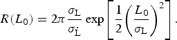 $$R({L_0}) = 2\pi \displaystyle{{{\sigma _{\rm L}}} \over {{\sigma _{\dot {\rm L}}}}}\exp \left[ {\displaystyle{1 \over 2}{{\left( {\displaystyle{{{L_0}} \over {{\sigma _{\rm L}}}}} \right)}^2}} \right].$$
where ${\sigma _{\dot {\rm L}}}$
is the standard deviation of the time rate of change of L. The curves in Figure 3 give everything needed to calculate R(L
0). Figure 4a shows that the expected return time of an advance past zero (i.e. equilibrium) is 42 a for white-noise forcing, increasing slightly with persistence to 58 a for ν = 0.4. However there is a dramatic reduction in the return time of large advances because Eqn (13) has an exponential sensitivity to σ
L. For instance, for our control glacier, a 1 km advance is expected to occur on average once every 20 ka for white noise, but once every 400 a for ν = 0.4 (Fig. 4a).
${\sigma _{\dot {\rm L}}}$
is the standard deviation of the time rate of change of L. The curves in Figure 3 give everything needed to calculate R(L
0). Figure 4a shows that the expected return time of an advance past zero (i.e. equilibrium) is 42 a for white-noise forcing, increasing slightly with persistence to 58 a for ν = 0.4. However there is a dramatic reduction in the return time of large advances because Eqn (13) has an exponential sensitivity to σ
L. For instance, for our control glacier, a 1 km advance is expected to occur on average once every 20 ka for white noise, but once every 400 a for ν = 0.4 (Fig. 4a).
(a) Return times of a given advance, as a function of climatic persistence, calculated from Eqn (13) for the control glacier parameters. Note the logarithmic y-axis. (b) Excursion probabilities as a function of climatic persistence. It shows the probability of exceeding a given total excursion (i.e. maximum minus minimum extent) in any 1 ka period of constant climate. Curves are calculated from Eqn (14) for the control glacier parameters. The presence of even a small degree of persistence can dramatically increase the likelihood of seeing a given excursion.

Another relevant metric is the probability of a given total excursion (i.e. maximum − minimum extent) in a given period of time, say 1 ka. It is useful to evaluate, for example, whether a given moraine might have been deposited simply because of internal climate variability, or whether the moraine must have required a climate change. Such calculations can also be used to correct estimates of past climate change from moraines records, recognizing that the moraines represent extrema in the lengths of fluctuating glaciers, and that the terminus position associated with the average climate during any given period likely lies somewhat up-valley (Anderson and others, Reference Anderson, Roe and Anderson2014; Rowan and others, Reference Rowan2014).
Using standard results from extreme-value statistics (e.g. Vanmarcke, Reference Vanmarcke1983), Roe (Reference Roe2011) derived the probability of a glacier exceeding a maximum total excursion, ΔL, in any given interval of time, ${\rm {\cal T}}$
, assuming the extreme-excursion return times following a Poisson distribution:
${\rm {\cal T}}$
, assuming the extreme-excursion return times following a Poisson distribution:
 $$\eqalign{& p({L_{max}} - {L_{min}} \gt \Delta L)({\rm {\cal T}}) = \cr & \quad \int_0^\infty {\Delta L \over R ({L_1})\sigma _{\rm L}^2} {e^{ - {{\cal T}}/R({L_1})}}\left( {1 - {e^{ - {\rm {\cal T}}/R({L_1}-\Delta L)}}} \right){\rm d}{L_1}.} $$
Figure 4b shows the probabilities of exceeding a given total excursion in any 1 ka period, calculated from the return times shown in Figure 4a. Including persistence has a dramatic impact. For instance, a 2 km excursion has only a 1% chance of happening for white noise, but a 98% chance of happening for ν = 0.4. These results represent a severe complication in evaluating whether a particular moraine on a landscape required a climate change or not, given that the degree of persistence we have used is hard to detect in mass-balance records: that is, the statistical inferences are acutely sensitive to some poorly constrained assumptions.
We note that the Poisson distribution governs events that occur independently, and that this is only an approximation when applied to total glacier excursions (i.e. both maxima and minima) and when climatic persistence is included. In other analyses (not shown) we found the Poisson distribution held well for 1 ka periods for ν < 0.5, but care should be taken applying the formula for shorter periods. Its validity depends on the glacier response time and the degree of climatic persistence. The three-stage model is simple enough that the validity of the assumption can always be checked using Monte Carlo methods.
3.2. Spanning a broad range of parameters
So far, we have used one standard set of glacier parameters and varied only the persistence. Figures 5a and b shows how σ L varies as a function of glacier timescale, τ g, and r or ν, using Eqns (7), (9), and (11); and recognizing that τ g for our control glacier (~7 a) is quite small relative to values estimated for many other glaciers (e.g. Leclercq and Oerlemans, Reference Leclercq and Oerlemans2012).
Contours of the standard deviation of glacier response σ L (m) as a function of glacier response time, τ g, and climatic persistence (either r or ν). (a) AR(1) persistence, r. (b) Power-law persistence, ν. For these calculations the value of β and σ b are held constant.

Increasing τ g increases σ L (i.e. Eqn 8). A longer glacier response time implies a weaker restoring tendency for a given L′ (e.g. Eqn 6), and so the glacier will undergo larger and longer excursions in response to stochastic forcing. The impact of persistence grows with τ g, more so for power-law persistence (i.e. Eqn 11) than for AR(1) persistence (i.e. Eqn 10). The reason is that a glacier with a larger τ g can be thought of as a low-pass filter with a lower-frequency cut-off than a glacier with a smaller τ g. The differences between the white-noise and power-law spectra increase as frequency decreases, and those lower frequencies contribute more to the variance of the large-τ g glacier than the small-τ g glacier. So for our control glacier with τ g ~ 7 a, going from ν = 0 to ν = 0.4 has a less than two-fold impact on σ L; however for τ g ~ 50 a the effect is nearly three-fold (Fig. 5b). Finally, we note that the strong sensitivity at larger values of ν is because of the dependence of σ L on secant (νπ/2) (i.e. Eqn 11), which reflects the fact that the variance can become unbounded for large enough ν (Eqn A13).
We have also held β and σ b constant. From Eqn (7) we see that σ L is linearly proportional to each of them, so our results can easily be applied to other glaciers by reading off the contours in Figure 5. It should also be noted that τ g and β are related via the glacier thickness, H (see the discussions in Section 3 after Eqn (6)).
4. SUMMARY AND DISCUSSION
Observational records of glacier mass balance are short, and this makes it hard to establish the degree of climatic persistence that pertains to them. Typically, they are short enough that the null hypothesis of no persistence (i.e. white noise) cannot be rejected. And yet there are other observational datasets and also theoretical grounds for being confident that a degree of climatic persistence does, in fact, exist. We have explored the impact of climatic persistence on glacier length fluctuations. For two different statistical models we have found that, even for a degree of persistence that is hard to detect in instrumental records, the magnitude of glacier length fluctuations can be significantly enhanced over that in the case of no persistence. The effect becomes even more important when one considers the impact on excursion probabilities. For extreme excursions, persistence can turn an ‘exceptionally unlikely’ event (<1%) into a ‘virtually certain’ event (>99%, using IPCC (Reference Stocker2013) definitions and a slight extrapolation from Fig. 4b).
Our results compound with the other challenges of identifying past climate change from the glacier length record. If one accepts that internal climate variability will produce stochastic fluctuations of glacier length then, ipso facto, identifying climate change in the glacial record is an exercise in signal-to-noise detection. In turn, such an exercise depends on our physical models for what the glacier ‘noise’ is. For most glaciers, observed mass-balance variability is not constrained to within a factor of two (Section 2.1). The alternative – modeling mass balance from meteorological data – relies on uncertain parameters, and in any event can only ever be calibrated and evaluated against the direct observations. Because the moraine record is intrinsically fragmentary, we must estimate glacier response to internal climate variability using models. In principle, analytical tools like the three-stage model of Roe and Baker (Reference Roe and Baker2014) are efficient vehicles for building intuition about the relative importance of forced and unforced climate variability. Many parameters are accurately observed, but some important parameters like glacier thickness, H, remain poorly constrained. Methodology is improving, but Huss and Farinotti (Reference Huss and Farinotti2012) report a standard error of ~30%. More comprehensive numerical models are not obviously more skillful, depending as they do, on uncertain rheologies and crude parameterizations of subglacial hydrology. In the present study, we have added to this litany of vexation by noting that persistence for glacier mass balance is poorly constrained, while demonstrating it can exert a large influence on the magnitude of glacier length fluctuations. Of course, there is no question but that the Pleistocene Ice Age constituted a climate change that left its mark on the moraine record, a conclusion that survives all modeling uncertainty (e.g. Anderson and others, Reference Anderson, Roe and Anderson2014; Rowan and others, Reference Rowan2014). However the interpretation of Holocene moraines, for which climate changes may be more marginal, is less clear. Events such as the putative Little Ice Age may not stand out relative to the noise of internal climate variability (e.g. Matthews and Briffa, Reference Matthews and Briffa2005).
What to do? In this study we have focussed exclusively on the magnitude of the fluctuations of an individual glacier, and we have made the case that, with existing observations, the minimum uncertainty in the magnitudes of the fluctuations due to internal climate variability remains a factor of two or three (at least until observational records grow long enough to constrain σ b better). However other information can also be brought to bear on interpreting glacier history. In particular, the spatial extent, or the temporal duration, of contemporaneous glacier length fluctuations can make for an independent test of a climate-change hypothesis. In other words, is the duration or spatial coherence of glacier length fluctuations surprising, given a null hypothesis that they are unconnected? The statistical machinery exists (e.g. Bretherton and others, Reference Bretherton, Widmann, Dymnikov, Wallace and Blad1999), to assess the spatial and temporal correlations in climate and glacier variability. Such tools have yet to be applied to interpreting the glacier record, and an important caveat is that the spatial coherence varies with timescale (e.g. Deser and others, Reference Deser, Alexander, Xie and Phillips2010; Meehl and others, Reference Meehl, Hu, Arblaster, Fasullo and Trenberth2013). However, some principles can be laid out. Glacier length fluctuations within individual mountain ranges will be highly coherent, since they experience essentially the same climate and so do not constitute independent records of climate change (e.g. Huybers and Roe, Reference Huybers and Roe2009). Observations and theory suggest that the degree of climatic persistence is likely greater for maritime settings than for continental settings (e.g. Pelletier, Reference Pelletier1997; Huybers and Curry, Reference Huybers and Curry2006). On larger spatial scales and longer timescales, interpretations of geologic observations hinge critically on the accuracy with which moraine dating can be made, and there is an ongoing and vibrant debate as to what is achievable (e.g. Davis and others, Reference Davis, Menounos and Osborn2009 and references therein; Balco, Reference Balco2009; Schaefer and others, Reference Schaefer2009; Kirkbride and Winkler, Reference Kirkbride and Winkler2012; Schimmelpfennig and others, Reference Schimmelpfennig2012; Solomina and others, Reference Solomina2015).
We have followed in the path of Reichert and others (Reference Reichert, Bengtsson and Oerlemans2002) by including persistence in the climate variability. Does such persistence by itself imply climate changes? In the case of AR(1) persistence, the answer is an emphatic no because the timescales are too short and reflect only, for example, the integrating effects of the ocean mixed layer. For power-law persistence the answer is a little more nuanced. Power-law variability is a constant climate in the sense that it requires neither changes in external forcing, nor changes to the dynamics of the climate system. However variability continues to increase out to lower frequencies and eventually merges into a portion of the spectrum that is most definitely a response to external forcing (e.g. Huybers and Curry, Reference Huybers and Curry2006). The fact the background spectrum of climate variability is a continuum means that what constitutes climate ‘change’ will always depend on somewhat arbitrary definitions.
A related question is whether climate variability is itself a function of mean state. If the climate change is large enough that there are significant shifts of major climatic zones, then there must, at some level, be changes in local variability, especially at the margins of those zones. However for the as yet relatively small climate changes of the last century (~1 K in the global mean), there are no theoretical grounds for expecting that changes in the variability (i.e. the second and higher-order moments of the statistical distribution) have had as big an impact as shifts in the mean (i.e. the first moment). This is largely borne out in observations and models (e.g. Simolo and others, Reference Simolo, Brunetti and Nanni2011; Donat and Alexander, Reference Donat and Alexander2012; Rhines and Huybers, Reference Rhines and Huybers2013). So while possible changes in variability are worth keeping in mind for the larger climate changes of past millennia, the modern instrumental record of variability provides a good foundation for building intuition about the impact of variability in past climates.
The amplitude and nature of internal climate variability is one of the most important challenges in climate science. It governs the predictability of future climate (e.g. Hawkins and Sutton, Reference Hawkins and Sutton2009; Deser and others Reference Deser, Phillips, Bourdette and Teng2012), and the interpretation and statistical significance of past changes, an example of which was our focus here. While we have concentrated on glaciers, the impact of climatic persistence on the response of all paleoclimate proxies is important to assess. There is currently a mismatch between the climatic persistence inferred from paleoclimate proxies and that generated by comprehensive climate models, which may reflect a problem with the proxy records, or the models, or both (Laepple and Huybers, Reference Laepple and Huybers2014). It remains to be seen what the resolution will be.
Appendix
IMPACT OF CLIMATIC PERSISTENCE ON THE STANDARD DEVIATIONS OF GLACIER LENGTH FLUCTUATIONS
The continuous form of the three-stage glacier model equation is:
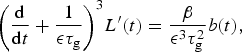 $${\left( {\displaystyle{{\rm d} \over {{\rm d}t}} + \displaystyle{1 \over {{\epsilon} {\tau _{\rm g}}}}} \right)^3}L^{\prime}(t) = \displaystyle{\beta \over {{{\epsilon} ^3}\tau _{\rm g}^2}} b(t),$$
The discrete version of the three-stage model (e.g. Roe and Baker, Reference Roe and Baker2014) is more closely analogous to the flowline numerical model (and to nature). However, for analytic tractability, we use the continuous equations here, and we also derive the glacier variance by integrating the power spectrum from 0 to ∞, rather than 0 to f 0. This approximation is justified since the continuous equations differ most from the discrete equations at high frequencies (f ≫ 1/τ g). These frequencies are strongly damped by the glacier dynamics, which thus minimizes the differences from the discrete equations. We also derive expressions for the ratios of the variances with-and-without persistence, and these ratios show close agreement with ratios computed from the numerical flowline model and the discrete three-stage model.
Since Eqn (A1) is a linear equation, we can seek Fourier-transform solutions of the form:
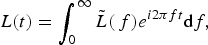 $$L(t) = \int_0^\infty \tilde L(\,f){e^{i2\pi ft}}{\rm d}f,$$
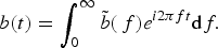 $$b(t) = \int_0^\infty \tilde b(\,f){e^{i2\pi ft}}{\rm d}f.$$
Substituting into Eqn (A1) gives
 $${\left( {i2\pi f + \displaystyle{1 \over {{\epsilon} {\tau _{\rm g}}}}} \right)^3}\tilde L(\,f) = \displaystyle{\beta \over {{{\epsilon} ^3}{\tau ^2}}}\tilde b(\,f).$$
Next, take the product of Eqn (A4) and its complex conjugate. Together with the definitions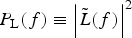 $P_{\rm L}(f) \equiv {\left\vert \tilde L(f)\right\vert}^2$
and
$P_{\rm L}(f) \equiv {\left\vert \tilde L(f)\right\vert}^2$
and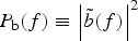 $P_{\rm b}(f) \equiv {\left\vert \tilde b(f) \right\vert}^2$
; this gives:
$P_{\rm b}(f) \equiv {\left\vert \tilde b(f) \right\vert}^2$
; this gives:
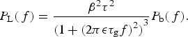 $${P_{\rm L}}(\,f) = \displaystyle{{{\beta ^2}{\tau ^2}} \over {{{(1 + {{(2\pi {\epsilon} {\tau _{\rm g}}f)}^2})}^3}}}{P_{\rm b}}(\,f).$$
This is a general expression that applies for any P b(f).
First, for a continuous AR(1) process, we set
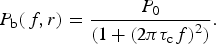 $${P_{\rm b}}(\,f,r) = \displaystyle{{{P_0}} \over {(1 + {{(2\pi {\tau _{\rm c}}f)}^2})}}.$$
(e.g. Box and others, Reference Box, Jenkins and Reinsel2008). We determine P
0 as follows: for white noise, ${P_0} = 2\Delta t\sigma _{\rm b}^2 $
, which gives
${P_0} = 2\Delta t\sigma _{\rm b}^2 $
, which gives $\int_0^{{f_0}} {P_{\rm b}}(f){\rm d}f = \sigma _{\rm b}^2 $
, where f
0 = 1/2Δt. For the discrete AR(1) power spectrum Eqn (2), the low frequency response is
$\int_0^{{f_0}} {P_{\rm b}}(f){\rm d}f = \sigma _{\rm b}^2 $
, where f
0 = 1/2Δt. For the discrete AR(1) power spectrum Eqn (2), the low frequency response is ${P_{\rm b}}{\vert_{f = 0}} = 2\Delta t\sigma _{\rm b}^2 /{(1 - r)^2}$
. Finally for a general discrete AR(1) process the variance is enhanced by a factor of 1/(1 − r
2) compared with white noise (e.g. Box and others, Reference Box, Jenkins and Reinsel2008). So to ensure the variance of our synthetic climate time series does not depend on the persistence we divide by this factor, giving:
${P_{\rm b}}{\vert_{f = 0}} = 2\Delta t\sigma _{\rm b}^2 /{(1 - r)^2}$
. Finally for a general discrete AR(1) process the variance is enhanced by a factor of 1/(1 − r
2) compared with white noise (e.g. Box and others, Reference Box, Jenkins and Reinsel2008). So to ensure the variance of our synthetic climate time series does not depend on the persistence we divide by this factor, giving:
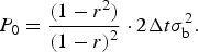 $${P_0} = \displaystyle{{(1 - {r^2})} \over {{{(1 - r)}^2}}} \cdot 2\Delta t\sigma _{\rm b}^2. $$
Equations (A6) and (A7) can be substituted into Eqn (A5), and integrated to calculate the variance $\sigma _{\rm L}^2 $
. It turns out there is an analytical solution that can be found from standard integral tables. After some manipulation:
$\sigma _{\rm L}^2 $
. It turns out there is an analytical solution that can be found from standard integral tables. After some manipulation:
 $$\sigma _{\rm L}^2 = \int_0^\infty {P_{\rm L}}(\,f){\rm d}f = \displaystyle{{(1 - {r^2})} \over {{{(1 - r)}^2}}} \cdot \displaystyle{{{\beta ^2}{\tau ^2}2\Delta t\sigma _{\rm b}^2} \over {32}} \cdot \displaystyle{{(3{{\epsilon} ^2}\tau _{\rm g}^2 + 9{\epsilon} {\tau _{\rm g}}{\tau _{\rm c}} + 8\tau _{\rm c}^2 )} \over {{{({\epsilon} \tau + {\tau _{\rm c}})}^3}}}.$$
Finally, we can define the ratio of the variances with-and-without persistence:
 $${R_r} = \displaystyle{{{{\left. {\sigma _{\rm L}^2} \right \vert} _r}} \over {{{\left. {\sigma _{\rm L}^2} \right \vert} _{r = 0}}}} = \displaystyle{{(1 - {r^2})} \over {{{(1 - r)}^2}}} \cdot \displaystyle{{{\epsilon} {\tau _{\rm g}}(3{{\epsilon} ^2}\tau _{\rm g}^2 + 9{\epsilon} {\tau _{\rm g}}{\tau _{\rm c}} + 8\tau _{\rm c}^2 )} \over {3({\epsilon} \tau + {\tau _{\rm c}}{)^3}}}.$$
Or in the limit of ετ g ≫ τ c, this becomes simply:
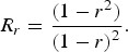 $${R_r} = \displaystyle{{(1 - {r^2})} \over {{{(1 - r)}^2}}}.$$
For power-law spectra, we have:
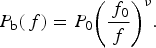 $${P_{\rm b}}(\,f) = {P_0}{\left( {\displaystyle{{{\,f_0}} \over f}} \right)^\nu}.$$
We set ${P_0} = (1 - \nu ) \cdot 2\Delta t{\sigma _{\rm b}}^2 $
, which ensures
${P_0} = (1 - \nu ) \cdot 2\Delta t{\sigma _{\rm b}}^2 $
, which ensures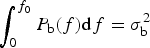 $\int_0^{{f_0}} {P_{\rm b}}(f){\rm d}f = \sigma _{\rm b}^2 $
. Upon substitution into Eqn (A5):
$\int_0^{{f_0}} {P_{\rm b}}(f){\rm d}f = \sigma _{\rm b}^2 $
. Upon substitution into Eqn (A5):
 $$\sigma _{\rm L}^2 = {\beta ^2}{\tau ^2}{P_0}f_0^\nu \int_0^\infty \displaystyle{{{\,f^{ - \nu}}} \over {{{(1 + {{(2\pi {\epsilon} \tau f)}^2})}^3}}}{\rm d}f.$$
This again turns out to have an analytic solution, which can be reduced to
 $$\sigma _{\rm L}^2 = \displaystyle{{{\beta ^2}\tau \Delta t\sigma _{\rm b}^2} \over {16\varepsilon}} {(2\pi {\epsilon} {\,f_0}\tau )^\nu} (1 - {\nu ^2})(\nu + 3)\sec (\nu \pi /2).$$
Hence the ratio of variances, R ν , can be written as:
 $${R_\nu} = \displaystyle{{{{\left. {\sigma _{\rm L}^2} \right \vert} _\nu}} \over {{{\left. {\sigma _{\rm L}^2} \right \vert} _{\nu = 0}}}} = \displaystyle{{{\pi ^\nu} {{({\epsilon} \tau /\Delta t)}^\nu} (1 - {\nu ^2})(\nu + 3)\sec (\nu \pi /2)} \over 3}.$$


 Open access

