


Nomenclature
- AEM
-
active energy management
- B
-
battery
- BMS
-
battery management system
- ${c_1},\;{c_2}$
-
personal and social learning coefficients
- DC
-
direct current
- ECMS
-
equivalent consumption minimisation strategy
- ESC
-
electronic speed controller
- FC
-
fuel cell
-
$F{E_{ref.}}$
-
endurance value for SMC algorithm
- FL
-
fuzzy logic
-
$gbest$
-
global best position
-
${h_i}$
-
proportional flight time contribution of algorithm i
-
$i$
-
particle
- J
-
objective function
-
$mbest$
-
best position of the swarm
- OB
-
optimisation-based
-
${P_{batt}}$
-
power of battery
-
${p_i}$
-
quantum optimal point
-
${P_{pv}}$
-
power of solar cells
-
$pbest$
-
personal best position
- PEMS
-
proton-exchange membrane
- PV
-
solar cell
- QPSO
-
quantum particle swarm optimisation
- RB
-
rule-based
- RF
-
radio frequency
-
${r_1},\;{r_2}$
-
random numbers, between 0 and 1
- SC
-
supercapacitor
- SOC
-
state of charge
-
${t_i}$
-
time reaching the maximum power of algorithm i
-
${t_{ref}}$
-
time reaching the maximum power of algorithm SMC
-
$u$
-
random number, between 0 and 1
-
${v_i}$
-
velocity probability centre
-
$w$
-
coefficient of inertia
-
${x_i}$
-
position


Greek symbol
- β
-
quantum scaling factor
- Δt
-
time step
1.0 Introduction
The propulsion systems of unmanned aerial vehicles (UAVs) are fundamentally classified into two categories: non-electric systems, which include jet and internal combustion engines, and electric-powered systems, which utilise fuel cells, solar cells or batteries [Reference Rehan, Akram, Shahzad, Shams and Ali1]. In recent years, UAVs with a take-off mass lower than 25 kg, which is generally categorised as small [Reference Kody and Bramesfeld2, Reference Eisenbeiss3], typically rely on electric propulsion systems due to being low emission [Reference Tian, Zhang, Zhou and Guo4], high energy conversion efficiency [Reference Amici, Ceresoli, Pasetti, Saponi, Tiboni and Zanoni5, Reference Feng, Li, Xue, Gao, Bai, Zhang and Guo6], scalability [Reference Boukoberine, Zhou and Benbouzid7], high stealth and low noise [Reference Tao, Zhou, Zicun and Zhang8]. Among these energy components, solar cells play a crucial role in enabling continuous energy generation without the need for landing, thereby significantly enhancing the flight time and endurance of UAVs [Reference Guo, Zhou, Wang, Zhao and Zhu9]. Consequently, solar cells are considered an essential energy source for small UAVs used in surveillance, reconnaissance and scientific data collection missions [Reference Romeo and Frulla10].
UAVs typically operate in various flight modes, such as hover, take-off, climb, cruise, descent and landing, each exhibiting distinct power consumption characteristics [Reference Abeywickrama, Jayawickrama, He and Dutkiewicz11]. For instance, take-off and hover require significantly higher power demands compared to other flight modes. Consequently, solar cells alone are insufficient to meet the energy requirements of these high-power-demand phases [Reference Gang and Kwon12, Reference El-Atab, Mishra, Alshanbari and Hussain13]. Moreover, solar cells are only operational during daylight hours. Despite their advantage of generating energy in flight, UAVs powered by solar cells rely on hybrid systems that integrate batteries, fuel cells and/or supercapacitors to ensure a continuous power supply. In these systems, batteries or supercapacitors compensate for instantaneous high energy demands, while solar cells provide power during lower-demand flight modes, such as cruising, thereby significantly extending flight duration. As a result, some solar-powered UAVs can remain operational for weeks. However, the efficiency of such hybrid systems depends on well-designed energy management strategies to optimise power distribution, enhance energy efficiency and ensure mission success through uninterrupted power supply during operation. Challenges such as real-time applicability, computational burden, overall system efficiency and performance under dynamic loads remain key research gaps in hybrid power system management [Reference Zhang, Qiu, Chen, Li, Liu, Liu, Zhang and Hwa14, Reference Xu, Huangfu, Ma, Xie, Song, Zhao, Yang, Wang and Xu15]. Addressing these gaps serves as the primary motivation for this study.
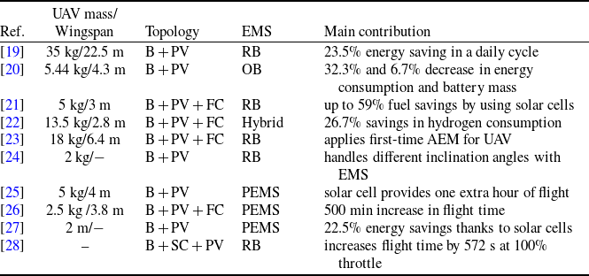
In recent years, a lot of research has been conducted on the energy management of solar-powered hybrid UAVs. These studies predominantly employ rule-based (RB) energy management due to their simple structure. However, some studies have implemented optimisation-based (OB) energy management, taking into account the trajectory of solar-powered UAVs [Reference Tian, Liu, Zhang and Yang16–Reference Tian, Liu, Zhang, Shao and Ge18]. This study’s motivation comes from the necessity for a comprehensive comparison of these energy management algorithms within the same system. Table 1 compares some highlighted studies on solar-powered UAVs in terms of energy management algorithm, topology and UAV mass/wingspan.
Studies on the energy management algorithms for solar cell-powered UAVs

To address the research gaps, this study applies FL, ECMS and QPSO algorithms for energy management in hybrid propulsion that uses a battery, supercapacitor and solar cell, comparing their efficiency. The comparison is conducted using the state machine control algorithm proposed in Ref. [Reference Engin, Çınar and Kandemir29] by the authors of this study as a benchmark. Additionally, the study in Ref. [Reference Engin, Çınar and Kandemir29] serves as a benchmark to evaluate the three algorithms in terms of their contribution to the UAV’s flight time. The optimisation problem formulated for energy management aims to minimise the total power consumed by the battery and solar power, while incorporating the operating limits of the battery and solar cell as constraints. Simulations are conducted in MATLAB/Simulink, where the energy components are managed by DC/DC converters. In summary, this study: (i) compares three optimisation-based algorithms in terms of their impact on maximum power and flight duration, (ii) applies the QPSO algorithm for the first time to a hybrid system comprising a battery, solar cell and supercapacitor, (iii) contrasts the RB energy management algorithm from Ref. [Reference Engin, Çınar and Kandemir29] with the OB algorithms used in this study and (iv) provides a comprehensive evaluation of the energy components and energy management strategies for a solar-powered UAV.
2.0 Methodology
2.1 UAV specification
Figure 1 illustrates the components of the solar-powered UAV modelled in this study. The UAV has a total mass of 3.3 kg; the battery and solar cells have masses of 1.3 kg and 256 g, respectively. This total mass comprises the solar cells, battery, electronic components (including the motor, propeller, etc.), cables, body, tail, the iron structure supporting the battery compartment and the protective varnish applied to the body and tail surfaces.
Hybrid UAV and components.

2.2 Hybrid power system architecture
In the hybrid power system, energy generation and consumption are dynamically monitored to ensure optimal power distribution according to flight conditions. Figure 2 shows the hybrid power topology of the small vertical take-off and landing (VTOL) UAV that runs on solar power [Reference Engin, Çınar and Kandemir29]. The components of this hybrid propulsion system are 32 solar cells, a lithium-polymer battery and a supercapacitor. Although the supercapacitor is integrated into the DC bus without any converter, the battery and solar cells are connected to its overall DC/DC converters.
2.2.1 Battery model
The MATLAB/Simulink library’s pre-existing model served as the basis for simulating the battery model used in this investigation [30]. A lithium-polymer battery with 8 Ah capacity and 14.8 V nominal voltage is modelled. A lithium-based battery is preferred due to its high energy density and long lifespan [Reference Zhang, Zhang, Li and Guo24].
In Fig. 3, during battery discharge, the voltage decreases as the capacity depletes, and this voltage drop accelerates when high current is drawn due to internal resistance. Over time, the battery voltage stabilises at a certain level and continues to decrease exponentially. This discharge curve is utilised in the energy management system to estimate the battery’s operational duration and charging time.
Hybrid power system topology.

The battery discharge curve.

The solar cell used in hybrid UAV.

2.2.2 Solar cell model
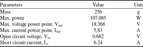
This study utilises the circuit model with a single diode, the most commonly used approach for estimating the generation of energy in solar cells. This model is accessible in the MATLAB/Simulink/Simscape library. In UAV applications, thin-film and silicon solar cells, as in Fig. 4, are frequently preferred [Reference Abbe and Smith31], because they offer advantages in terms of efficiency, weight, cost and feasibility [Reference Gao, Hou, Guo and Chen32]. The parameters of the solar cells listed in Table 2 are obtained from the datasheet issued by the manufacturer [33].
Parameters of solar cells (32pcs)

To maximise electricity generation from a solar cell, it must operate in regions close to the maximum power point. Therefore, solar cell systems require maximum power point tracking (MPPT). The variation of the hybrid power system’s solar cell array in terms of voltage, current and power characteristics is calculated as shown in Fig. 5 [30].
The characteristics of solar cell array.

2.2.3 Supercapacitor model
This study’s supercapacitor model can be found in the MATLAB/Simulink library, and simulations are run using it [30]. A supercapacitor with a capacity of 7 F and nominal voltage of 25 V is modelled.
The voltage of the supercapacitor is directly proportional to the amount of stored charge. The larger the capacitance, the smaller the voltage variation for a given charge. During the charging process, both voltage and current increase linearly, while during discharging, they decrease linearly until the supercapacitor is fully depleted.
2.2.4 DC/DC converter model
Through the use of converters, the energy management unit allocates the necessary power among energy sources in the most efficient manner. A two-way DC/DC converter is used in order to charge and discharge batteries, as well as for energy storage, as seen in Fig. 6. These converters manage the charge and discharge processes according to the energy source’s state of charge and the direction of current flow [Reference Alazrag and Sbita34]. During daylight, the energy harvested by the solar cells charges the battery via the DC/DC converter. When solar energy is unavailable, the battery discharges through the converter to deliver power to the system.
Circuit of the DC/DC bidirectional converter.

2.3 Definition of energy management problem
In this study, energy management algorithms developed for the solar-powered small-VTOL UAV were analysed using both RB and OB methods. The RB approach ensures real-time applicability with low computational load, while the OB approach aims for the efficient and effective utilisation of energy sources.
The flowchart of the power-sharing algorithm is presented in Fig. 7 [Reference Yavasoglu, Shen, Shi, Gokasan and Khaligh35]. In the hybrid power system, energy generation and consumption are dynamically monitored to enable power distribution according to flight conditions.
Flowchart of the power-sharing algorithm.

The MATLAB/Simulink system was used to carry out simulation studies [36]. The development of solar cell [37], battery [38] and supercapacitor [39] models was carried out using the MATLAB/Simulink (R2023b) library. Additionally, the functions of the implemented algorithms were written using function blocks in MATLAB/Simulink and integrated into the simulation system.
2.4 Energy management system design
The objective function is formulated to optimise the energy management strategy, as defined in Equation (1). The $\left( {SOC \times {\rm{\;}}{P_{batt}}} \right)$
term regulates battery utilisation based on the state of charge, preventing overcharging and deep discharging. The time scale multiplier (Δt) enables the assessment of total energy consumption on a temporal basis. The function aims to optimise battery usage by efficiently utilising solar energy.
$\left( {SOC \times {\rm{\;}}{P_{batt}}} \right)$
term regulates battery utilisation based on the state of charge, preventing overcharging and deep discharging. The time scale multiplier (Δt) enables the assessment of total energy consumption on a temporal basis. The function aims to optimise battery usage by efficiently utilising solar energy.
 \begin{align}J = ( {{P_{pv}} + ( {SOC \times {\rm{\;}}{P_{batt}}} )} ) \times \Delta t \end{align}
Fuzzy logic algorithm state diagram.

Equations (2), (3), (4) and (5) define the constraints of the problem. Equation (2) limits the max. and min. power values of the solar cells. The state of charge (SOC) of the battery is regulated by Equation (3). Equation (4) constrains the min. power and max. power levels of the battery. Similarly, Equation (5) imposes voltage limitations on the system.
 \begin{align} {P_{pv\_min}} &\le {P_{pv}} \le {P_{pv\_max}} \\[-8pt] \nonumber \end{align}
 \begin{align} SO{C_{min}} &\le SOC \le SO{C_{max}} \\[-8pt] \nonumber\end{align}
 \begin{align} {P_{bat\_min}} &\le {P_{bat}} \le {P_{bat\_max}}\\[-8pt] \nonumber \end{align}
 \begin{align} {V_{dc - dc\_input\_min}} &\le {V_{dc}} \le {V_{dc - dc\_input\_max}} \\[2pt]\nonumber \end{align}
2.4.1 Fuzzy logic controller
Fuzzy logic (FL) is a technique used to establish a specific input-output relationship and resolve uncertainties and complexities in power distribution among energy sources within the system [Reference Suryoatmojo, Mardiyanto, Riawan, Setijadi, Anam, Azmi and Putra40–Reference Zadeh42]. The complex and variable nature of solar energy, batteries and other energy sources often renders conventional control methods insufficient. Therefore, FL is preferred among RB energy management strategies to enable more dynamic and accurate power distribution.
In the flowchart presented in Fig. 8, power demand, DC converter voltage and current and battery SOC are considered as input parameters. Initially, the control loop is initiated by setting the system’s initial parameters. Then, real-time measurements and calculations from the system are processed, and input values are evaluated to verify control conditions. The FL control strategy processes these input values to regulate the system’s energy management.
Accordingly, the power, voltage and current of the battery are measured. Given that the battery and power demand values, the required current from solar cells is dynamically adjusted. The energy generated by the solar cells is transferred to the DC converter to meet the system’s requirements. This approach ensures the efficient management of energy sources and enhances the system’s adaptability to different operating conditions.
ECMS algorithm state diagram.

2.4.2 Equivalent energy consumption controller
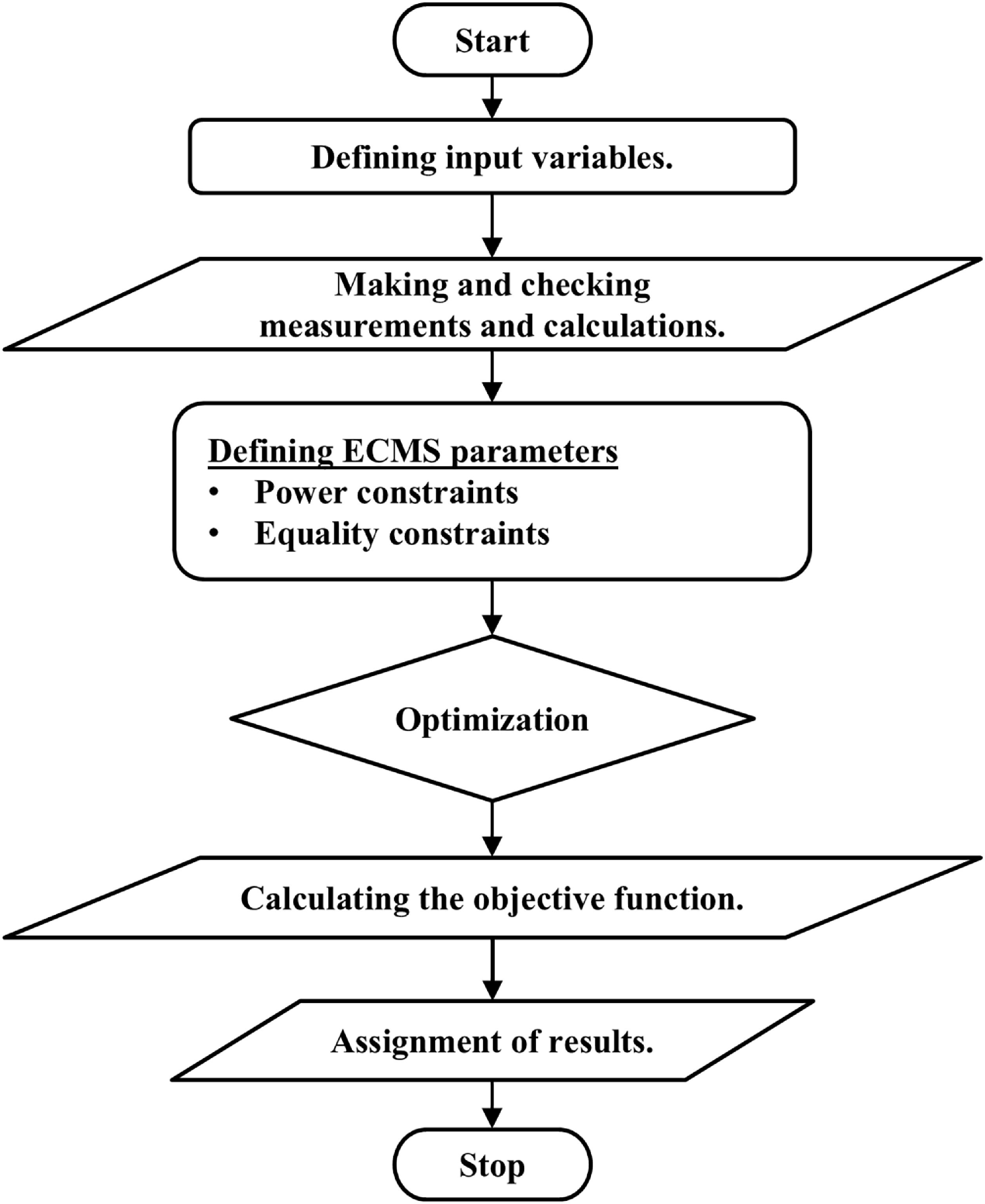
The equivalent consumption minimisation strategy (ECMS) is a non-metaheuristic, optimisation-based, real-time control method designed to achieve an optimal balance in energy management for hybrid UAVs [Reference Lei, Yang, Lin and Zhang43]. In this study, the ECMS states are defined according to Fig. 9 as follows:
-
• Input variables are defined to represent the instantaneous energy demands of the system and the status of available energy sources.
-
• Measurements and calculations are performed based on these variables. The system’s operating conditions are assessed, and the necessary data for energy management are collected.
-
• Equality constraints and power constraints are established. These constraints define the optimisation domains by considering the capacities of energy sources and the system’s load requirements.
-
• The optimisation process is executed, aiming to maximise the efficient utilisation of the system’s energy sources.
-
• One of the fundamental steps in ECMS is the calculation of the objective function, which is worked out to decrease energy consumption and maintain a balance between energy production and utilisation.
-
• The optimal solution values obtained from the optimisation process are assigned to the system parameters, and energy management is conducted accordingly.
2.4.3 Quantum particle swarm optimisation
Quantum particle swarm optimisation (QPSO) is an enhanced version of the classical PSO algorithm, developed based on quantum mechanics principles. It was first introduced by Sun et al. in 2004 [Reference Sun, Xu and Feng44, Reference Omkar, Khandelwal, Ananth, Narayana Naik and Gopalakrishnan45]. In this algorithm, each particle moves within a quantum potential well, characterised by parameters such as velocity and position, with positions determined by probability distributions.
Particle swarm optimisation (PSO) and QPSO are nature-inspired heuristic algorithms. PSO performs optimisation by updating the velocity and position of particles within the search space, whereas QPSO utilises quantum mechanics principles, allowing particles to move probabilistically around the global best solution. While PSO relies on Newtonian mechanics, QPSO allows particles to move within a quantum potential well.
The fundamental Equation (6) of PSO is as follows:
 \begin{align}&x_i^{t + 1} = x_i^t + v_i^{t + 1} \nonumber \\v_i^{t + 1} = wv_i^t + {c_1}{r_1}&\left( {pbes{t_i} - x_i^t} \right) + {c_2}{r_2}\left( {gbest - x_i^t} \right) \end{align}
On the other hand, in QPSO, particles move within a quantum potential well, and their positions are updated according to the following Equation (7):
 \begin{align}x_i^{t + 1} = {p_i} \pm \beta& \left| {mbest - } \right.\left. {x_i^t} \right|ln\left( {\frac{1}{u}} \right) \nonumber \\mbest &= \frac{1}{N}\mathop \sum \limits_{i = 1}^N pbes{t_i} \end{align}
Here, ${p_i}$
represents a point between the particle’s optimal position both globally and personally, while
${p_i}$
represents a point between the particle’s optimal position both globally and personally, while $mbest$
is the mean best position of all particles.
$mbest$
is the mean best position of all particles.
PSO provides a simpler and computationally less expensive optimisation approach, while QPSO enhances global optimisation capabilities and ensures faster convergence [Reference Huang, Fei and Deng46], particularly for complex and high-dimensional problems.
QPSO requires fewer iterations to reach a solution, making it convenient for real-time energy management applications. Also, it can better adapt to dynamic environmental conditions, such as variations in solar energy generation. As an OB and heuristic strategy, QPSO provides a rapid and effective solution for improving energy efficiency.
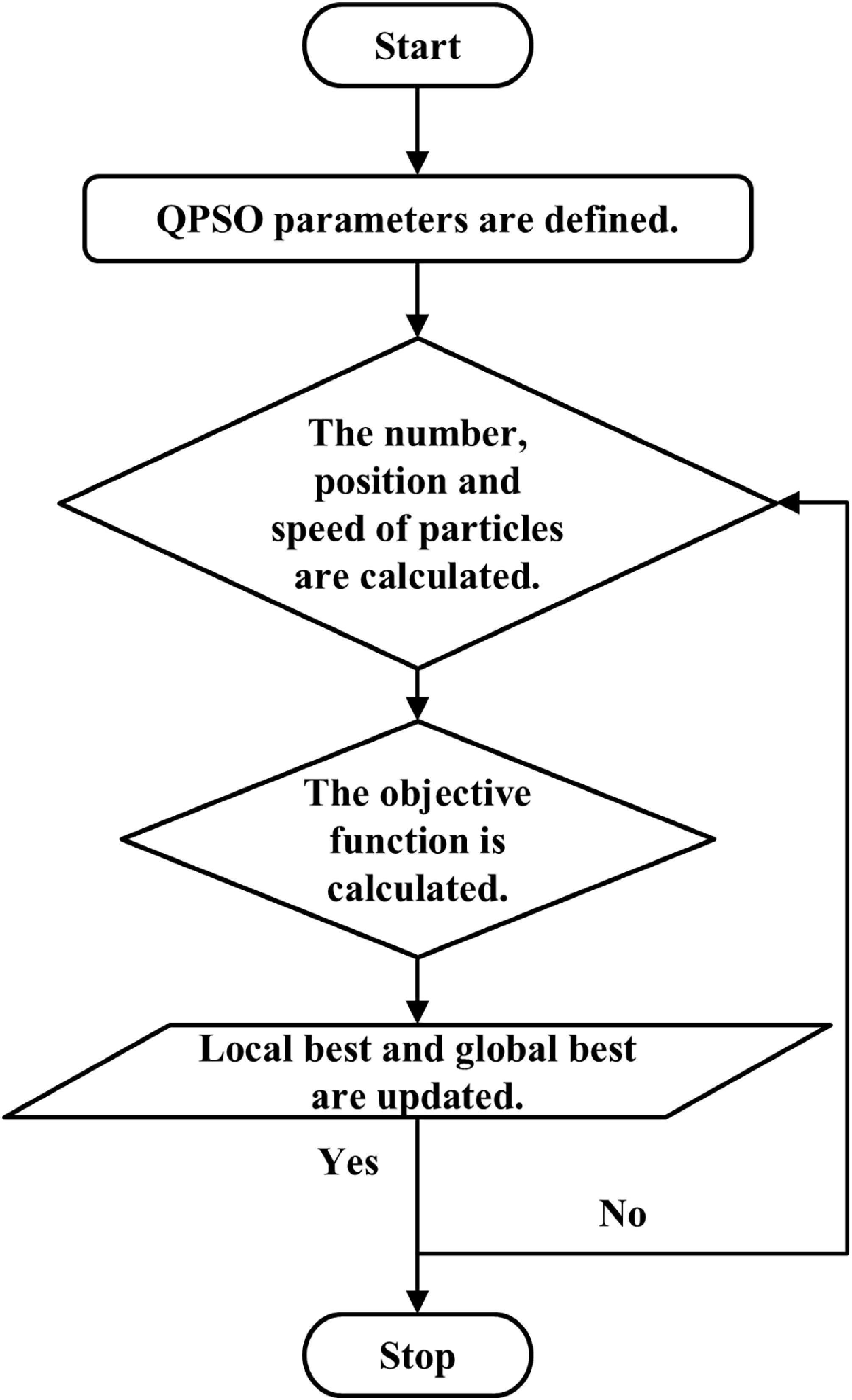
In this study, the states of the QPSO algorithm are defined according to Fig. 10 as follows:
-
• The fundamental parameters used in the optimisation algorithm are defined, including the number of particles, their initial positions and their velocities.
-
• The number, positions and velocities of the particles are calculated. The particles are randomly distributed within the solution space to address the energy management problem, and these positions serve as the starting point for the optimisation process.
-
• Each particle’s performance is evaluated by calculating the objective function. The objective function is a mathematical expression designed to optimise energy efficiency and the utilisation of energy resources by achieving a predefined target.
-
• Throughout the optimisation process, the local best value for each particle and the global best value among all particles are continuously updated. These updates enable the particles to regulate their positions and velocities to explore better solutions. The quantum properties of the QPSO algorithm allow particles to search for possible positions across a broader solution space, preventing the system from becoming entrapped in local minimum and facilitating convergence to the optimal solution.
QPSO algorithm state diagram.

2.5 Demand power calculation
The test setup shown in Fig. 11 was used to select a motor-propeller system compatible with the hybrid power system. As a result of the tests, thrust, current, power and efficiency data were obtained for the selected motor to ensure high thrust during VTOL. Accordingly, the propeller diameter and pitch were selected to achieve maximum efficiency with minimal power consumption during cruise and descent modes. Figure 12 illustrates the power demand profile of the hybrid-propulsion VTOL UAV, which was developed in Ref. [Reference Engin, Çınar and Kandemir29] based on the characteristics of the selected motor. The demand power was determined using an approach consistent with numerous studies in the literature [Reference Kim and Kang47, Reference Anderson48] in order to evaluate the performance of energy management algorithms using general flight performance equations. The power demand profile represents discretised mission phases defined for energy management evaluation rather than a continuous aerodynamic flight profile. Depending on the UAV’s modes of operation, take-off, climb, cruise, descent and landing, different thrust power requirements apply.
Engine-propeller test setup.

Power demand calculation for hybrid propulsion system (adapted from Ref. [Reference Engin, Çınar and Kandemir29]).

3.0 Result and discussion
3.1 Results of QPSO algorithm
Due to insufficient power output from the solar cells to supply the overall demand power, the battery’s SOC, which was initially at 80%, dropped to 79.87% between the 10th and 20th s in Fig. 13. The most power that could be extracted from the battery during this time was about 108 W. Since the solar cells’ power output surpassed the necessary demand, the battery was no longer used after the 20th second. Furthermore, it was noted that the battery current fluctuated between −25 A and 6.78 A. Here, the charging current drawn by the system-integrated supercapacitor causes the battery current to start at −25 A.
Battery SOC, current and power changes in the QPSO algorithm.

Supercapacitor SOC, current and power changes in the QPSO algorithm.

In Fig. 14, the supercapacitor’s initial charge level was 98%, and the power variation during the simulation ranged between −20 W and 178 W. Notably, between the 100th and 130th s, the system was not powered by the supercapacitor. Instead, its SOC went up due to power intake from other sources of energy. Throughout the simulation, the current passing through the supercapacitor varied between −1 A and 25 A.
The changes in the DC bus voltage, DC bus current and battery-DC converter input voltage are shown in Fig. 15. The simulation results indicate that the DC bus voltage varied between 15.8 V and 25 V, the DC bus current fluctuated between 0 and 12.5 A and the DC converter input voltage stayed at 15.8 V. These variations in DC bus current and voltage suggest that the power flow within the system was managed in a stable and balanced manner.
DC bus voltage and current and the input voltage of the battery–DC converter in the QPSO algorithm.

Voltage, current and power changes of solar cells in the QPSO algorithm.

The power changes in the QPSO algorithm.

In Fig. 16, the current, voltage and power variations of the solar cells are presented. The voltage remained constant at 15.8 V, while the output current ranged between 0 and 4.5 A. The solar cells’ power output peaked at 77 W at the tenth second. Figure 17 provides a detailed representation of the power-sharing processes during the simulation. In the first 10 s, the required power is supplied by the solar cells and the supercapacitor. Subsequently, the maximum demand for power was satisfied solely by the solar cells. Between the 15th and 20th s, a reduction in power demand was observed, during which energy was supplied by both the solar cells and the battery. The solar cells produced more power than was needed after the 20th s. In this model, altitude (gravitational potential) energy is treated as a dynamic energy storage mechanism governed by the system power balance, rather than a prescribed flight trajectory. This excess power is stored in the system in the form of altitude (gravitational potential) energy, consistent with the modelling approach presented in Ref. [Reference Engin, Çınar and Kandemir29]. The stored altitude (gravitational potential) energy is utilised to charge the supercapacitor during the time intervals of 40th–60th s and 100th–130th s. Any remaining excess energy continues to be stored as altitude energy. The stored altitude energy is subsequently utilised to support the charging of the supercapacitor and the battery.
3.2 Comparison of different controllers
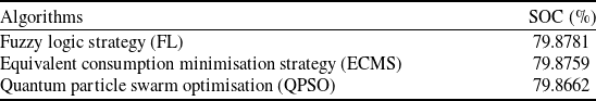
Initially, the battery’s SOC was at 80%. As illustrated in Fig. 18, between the 10th and 20th s, energy was drawn from the battery due to the inability of the solar cells to meet the energy demand alone. During this period, the effects of different energy management algorithms on battery performance were analysed, and SOC values at the 20th s were calculated, as presented in Table 3.
Impact of algorithms on battery SOC

The results indicated that the most efficient algorithm in terms of battery consumption was QPSO. The SOC differences between FL and QPSO and ECMS and QPSO were determined as 0.0119% and 0.0097%, respectively. These findings highlight that the QPSO algorithm provides lower energy consumption compared to other algorithms.
Battery SOC comparison chart.

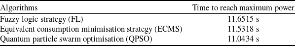
Figure 19 presents the variation in battery power over time due to energy withdrawal between the 10th and 20th s. Since the power that the solar cells generated was enough to meet the demand without the need for battery support, the battery was turned off at the 20th s. For all algorithms, the battery’s maximum power consumption was approximately 108 W. The time required for different algorithms to reach maximum power values is provided in Table 4.
Time taken for algorithms to reach maximum battery power

SOC effects of algorithms on supercapacitor

Additionally, the results demonstrate that QPSO reaches the maximum power value faster than the other algorithms, allowing it to respond more effectively to dynamic power demands. Specifically, QPSO achieved maximum power 0.5608 s faster than FL and 0.4581 s faster than ECMS.
Battery power comparison chart.

These results demonstrate that QPSO not only decreases energy consumption but also enhances the system’s speed of reaction to power demands.
As shown in Fig. 20, the supercapacitor SOC decreased from its initial value of 98 to 63% within the first 12 s of the simulation. This decline is attributed to the high energy demand at the beginning of the simulation, which necessitated energy supply from the supercapacitor. During this period, the supercapacitor served as the main energy source since the solar cells could not keep up with the demand for energy. The time required for SOC depletion under different energy management algorithms is presented in Table 5.
Supercapacitor SOC comparison chart.

QPSO completed the SOC depletion 0.6081 s earlier than FL and 0.4884 s earlier than ECMS. The ability of the QPSO algorithm to balance the supercapacitor load in a shorter time frame highlights its advantage in dynamic energy management.
Supercapacitor power comparison chart.

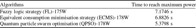
Figure 21 illustrates that the power fluctuation of the supercapacitor during the simulation ranged from −25 W to 178 W. The response of the supercapacitor to power demands and the influence of different energy management algorithms on this response were analysed based on the time required to reach the maximum power value, as detailed in Table 6. The results indicate that QPSO reached maximum power significantly faster than the other algorithms. Specifically, QPSO achieved maximum power 1.7948 s faster than FL and 1.5028 s faster than ECMS. This finding underscores the superior dynamic response capability of QPSO, enabling it to handle sudden power demands more efficiently.
Time taken by the algorithms to reach the maximum supercapacitor power

During the simulation, the supercapacitor did not supply power to the system between the 40th–60th and 100th–130th s. However, its SOC increased due to energy intake from other components. This observation confirms that the energy management system effectively facilitated the recharging of the supercapacitor while maintaining system stability. The passive role of the supercapacitor during these intervals indicates that other energy sources efficiently provided power to the system.
Overall, the findings show that QPSO performs better than other algorithms in achieving maximum power more rapidly, thereby enhancing the overall energy management performance. Furthermore, the observed SOC increase during the periods when the supercapacitor was not supplying power highlights the critical role of other energy sources in load balancing.
Figure 22 illustrates the power variation of the solar cell under different energy management algorithms. During the simulation, the maximum power output of the solar cell was 77 W.
Solar cell power comparison chart.

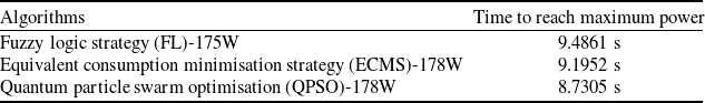
In the literature, the performance of energy management strategies has been comparatively analysed by considering the proportional contributions of their impacts on energy consumption and efficiency [Reference Zhang, Zhang, Li and Guo24]. In a similar manner, this approach enables the assessment of the relative contributions of different algorithms to flight endurance. The time required to achieve this peak power level varied depending on the algorithm used, as detailed in Table 7.
The duration of the algorithms to reach maximum power of the solar cell

Among the applied methods, the QPSO algorithm provides the fastest response to energy demand. According to Ref. [Reference Engin, Çınar and Kandemir29], the SMC algorithm increases flight endurance by 1.79 h.
Accordingly, a proportional calculation method expressed by Equation (8) is used to determine the contribution of the time required to reach maximum power to the total flight endurance for all algorithms. These endurance values ( ${h_i}$
) obtained from Equation (8) should be interpreted as proportional allocations of reference endurance improvement rather than as direct physical gain derived from response-time differences. In other words, reaching maximum power earlier allows solar energy to be integrated into the system at a higher level and for a longer period of time, resulting in a cumulative effect that delays battery discharge over the service life. The denominator
${h_i}$
) obtained from Equation (8) should be interpreted as proportional allocations of reference endurance improvement rather than as direct physical gain derived from response-time differences. In other words, reaching maximum power earlier allows solar energy to be integrated into the system at a higher level and for a longer period of time, resulting in a cumulative effect that delays battery discharge over the service life. The denominator $\sum ({t_i} - {t_{ref.}})\;$
represents the total response-time span of seconds and serves solely as a normalisation factor for proportional allocation. The reference endurance value
$\sum ({t_i} - {t_{ref.}})\;$
represents the total response-time span of seconds and serves solely as a normalisation factor for proportional allocation. The reference endurance value $F{E_{ref.}} = 1.79$
h is adopted from Ref. [Reference Engin, Çınar and Kandemir29], and
$F{E_{ref.}} = 1.79$
h is adopted from Ref. [Reference Engin, Çınar and Kandemir29], and $h_i$
denotes each algorithm’s relative endurance contribution in hours, obtained by scaling its response-time advantage against this span.
$h_i$
denotes each algorithm’s relative endurance contribution in hours, obtained by scaling its response-time advantage against this span.
 \begin{align}{h_i} = \frac{{{t_i} - {t_{ref.}}}}{{\sum ({t_i} - {t_{ref.}})}} \times F{E_{ref.}} \end{align}
where the subtitle i is the algorithm type, subtitle ref. represents the value for the SMC algorithm in Ref. [Reference Engin, Çınar and Kandemir29] and FE is the proportional time contribution for endurance in the Ref. [Reference Engin, Çınar and Kandemir29].
The time required for the QPSO algorithm to reach maximum power is significantly shorter compared to other algorithms. Specifically, the QPSO algorithm achieves this target 0.756 s faster than FL, and 0.465 s faster than ECMS. These results demonstrate that the QPSO algorithm responds more rapidly to energy demands and adapts more effectively to the system’s dynamic requirements. This graphical representation serves as a strong reference for the comparative evaluation of the potential of different algorithms in utilising solar energy within energy management systems.
3.3 Overall efficiency and stress analysis
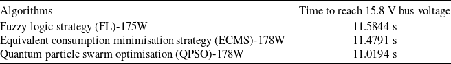
As illustrated in Fig. 23, the DC/DC bus voltage varied between 15.8 V and 25 V within the first 11 s of the simulation. The time required to reach a DC bus voltage of 15.8 V was analysed for different energy management algorithms and is presented in Table 8. The results indicate that the QPSO algorithm achieved the target voltage faster than the other algorithms with a time advantage of 0.5650 s over FL and 0.4597 s over ECMS.
Time taken for algorithms to reach bus voltage

These findings further emphasise the superior dynamic response capability of the QPSO algorithm. Its rapid response time enables more efficient handling of energy demands and facilitates quicker stabilisation of DC bus voltage fluctuations.
DC bus voltage comparison chart.

The solar cell-DC converter input voltage was observed to be 15.8 V when using the QPSO, whereas it was recorded as 15 V for the FL and ECMS algorithms. During system operation, in accordance with the energy management strategy, solar cells provided additional power from the battery and supercapacitor when required to meet the power demand. This process resulted in power fluctuations during the first 12 s of operation.
The observed difference in input voltage levels can be attributed to several factors. QPSO’s enhanced global search capability enables more efficient optimisation of the energy management strategy, leading to a more stable input voltage. Further, unlike FL and ECMS approaches, QPSO continuously adapts to system dynamics, allowing for more precise control of voltage levels.
4.0 Discussion and limitation
This study presents a comparative analysis of fuzzy, ECMS and QPSO energy management strategies implemented on a solar-based hybrid-powered UAV. The comparative results clearly demonstrate that energy management strategies play a critical role in determining how efficiently harvested solar energy is utilised and how effective the time to reach DC bus voltage and the time to reach maximum power. The time required for the solar cell to reach its maximum power of 77 W and the benchmark study in Ref. [Reference Engin, Çınar and Kandemir29] were considered to compare the energy management algorithms examined in this study. Their contributions to the UAV’s flight time were then computed proportionally. Based on these calculations, the FL, ECMS and QPSO algorithms contributed relatively 0.06 h, 0.51 h and 1.22 h to the endurance period, respectively. Consequently, the results indicate that the QPSO strategy, which is an optimisation-based approach, outperforms RB and heuristic methods in terms of maximising solar energy utilisation and extending flight endurance.
Notwithstanding these contributions, a few restrictions need to be taken into account. First, the study is based on a UAV configuration having less take-off weight, including fixed solar cell characteristics, battery and supercapacitor models and predefined mission and flight profiles. Even so, these presumptions allow for a controlled and equitable comparison of energy management techniques. However, the results of this study might not be directly expandable to UAVs with different sizes or mission profiles. Second, the simulations were carried out under idealised and structured operating conditions, presuming well-defined charge–discharge cycles and predictable solar irradiance. Due to weather, partial shading, changes based on flight attitude and dynamic mission profiles, solar energy availability may vary considerably during UAV real-time flights. Future research could examine these environmental parameters, which may have an impact on the evaluated energy management strategies’ real-time performance. Thirdly, even though optimisation-based energy management techniques provide adequate simulation performance, hardware constraints should be taken into account when assessing their computational burden. Hybridisations with RB energy management techniques can be taken into consideration to lessen computational burden. Lastly, only the simulation results in Ref. [Reference Engin, Çınar and Kandemir29] were used to validate the suggested energy management framework. To further confirm the efficacy and resilience of the suggested strategies, experimental flight tests conducted in actual environments would be beneficial. The findings will be more broadly applicable if the simulations are expanded to include battery ageing and various environmental conditions.
Lastly, this study shows that choosing and designing energy management strategies is crucial to the performance of solar-powered UAVs. Future research addressing this study’s conclusions will help develop more reliable, effective and workable energy management systems for long-range solar-powered UAVs.
5.0 Conclusion and future works
This study compares FL, ECMS and QPSO algorithms for the management of energy in a solar-powered small UAV. The UAV’s propulsion system consists of a solar cell, a battery and supercapacitors to meet sudden load demands. Additionally, energy management in this hybrid system is regulated by DC/DC converters. To evaluate the performance of these algorithms, the UAV’s propulsion system is modelled and simulated in MATLAB/Simulink.
The results demonstrate that the QPSO algorithm enables faster energy management than the other algorithms, significantly enhancing the endurance period. Additionally, the efficiencies of the FL, ECMS and QPSO algorithms were compared by considering the time required to reach maximum power and using the benchmark study. The findings indicate that the efficiencies of the FL, ECMS and QPSO algorithms were 0.44, 3.61 and 9.13% higher than that of the state machine control (SMC) algorithm in the benchmark study, respectively. These results suggest that algorithms capable of reaching maximum power more quickly are more efficient in utilising energy resources effectively.
In this study, only the UAV’s propulsion system model was used to provide a clearer comparison of energy management algorithms. In future works, the UAV’s flight model can be incorporated to explore long-range operation without energy consumption by utilising wind speeds at different altitudes through dynamic gliding combined with route planning. Additionally, improvements in aerodynamic design, such as wing morphing or an expandable wing profile, can be considered alongside energy management strategies.
Data availability statement
Data will be made available on request.
Acknowledgements
This study was funded by the Council of Higher Education 100/2000 Doctoral Scholarship Programme. Furthermore, the first author’s doctoral thesis served as the basis for this investigation.
Competing interests
The authors declare that they have no known competing financial interests or personal relationships that could have appeared to influence the work reported in this paper.


 Open access