
1 Introduction: The Purpose and Scope of This Element
This Element is intended to extend Bayesian statistical knowledge beyond the basics. In the companion volume (Gill & Bao, Reference Gill and Bao2024) we introduced the core concepts of Bayesian inference and the mechanics for estimating simple quantities from social science data, including basic probability theory, the likelihood function, the core principle of Bayesian inference, construction of priors, expected value, and model evaluation. Here we broaden those ideas and focus on Bayesian regression modeling. New topics include Monte Carlo, Markov chains, Markov chain Monte Carlo, linear and nonlinear (generalized linear) regression, the Bayes factor, and model assessment with simulation. This is how the bulk of empirical social science work is done, so we call this work “Getting Productive.” We extend the “Getting Started” principles from Gill and Bao (Reference Gill and Bao2024) here to this regression setting. Readers will get an appreciation for how the prior-to-posterior process works for common regression models that are linear, applied to dichotomous outcomes, applied to count outcomes, requiring bounded outcomes, and more.
Recall that the Bayesian statistical paradigm is perfectly suited to the type of data analysis routinely performed by social scientists since it recognizes that population parameters are not typically fixed in studies of humans, it incorporates prior knowledge from a specific literature, and it updates model estimates as new data are observed. Most empirical work in the social sciences is observational rather than experimental, meaning that there are additional challenges. Specifically: subjects are often uncooperative or not widely available, underlying systematic effects are typically more elusive than in the natural sciences, and measurement error is often significantly higher. The Bayesian approach to modeling uncertainty in parameter estimates provides a more robust and realistic picture of the data generating process because it is focused on estimating distributions rather than artificially fixed point estimates.
In Gill and Bao (Reference Gill and Bao2024) the key technical skill that needed to be introduced was calculus. More specifically, integral calculus so that expected value calculations and marginalizations could be done. The key technical skill introduced here is integration with Markov chain Monte Carlo (MCMC). This is actually a computational method for not doing integral calculus because the computer does the hard and repetitive work for integrals that are very difficult or even impossible to calculate analytically. In fact, MCMC liberated the Bayesians in 1990 (more details later in Section 4.2, “Markov Chain Theory”) and allowed us to specify regression-style models that were previously unavailable for primarily calculus reasons. In essence, we let the computer explore a large multidimensional space and report its traversal, which is in proportion to the posterior probability when set up correctly. So, much of the work here is computational because computation freed the Bayesians.
The notation here is identical to Gill and Bao (Reference Gill and Bao2024), but readers who have gained an appreciation for basic Bayesian inference from other sources will recognize the standard terms and formats used. We assume that current readers have seen and understood basic probability principles and Bayes’ law, likelihood functions, the core Bayesian process of generating posterior distributions from combining prior and likelihood (data) information, the role of priors in developing progressive science, integral calculus and expected value, calculating basic Bayesian quantities in R or Python, and evaluating/comparing model results. For extended details one can also reference Gill (Reference Gill2014).
The basic regression-style structure we will work with looks like this:
 (1.1)
(1.1)
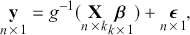
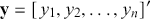
where  is a vector containing some outcome variable that can be measured as continuous or discrete,
  is an “inverse link function” that is specified according to the measurement of
  ,
,  is a matrix of explanatory variable data organized where rows are cases and columns are variables (including a leading column of 1s for the constant), and
  is the residual vector. Gill and Torres (Reference Gill and Torres2019) provide a detailed and accessible introduction to such model specifications in the non-Bayesian context. These are vector and matrix structures where the dimensions are specified with the underset text in (1.1), meaning that the
  and
and  vectors have
  contained cases, the
  matrix has
  cases and
  explanatory variables, and the
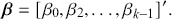
  vector has
  coefficients to be estimated. In order to make these multidimensional structures more visually intuitive, we repeat these specifications with illustration. The vector
  contains values of the outcome variable in a column vector:
 (1.2)
(1.2)
(the “prime” at the end of this statement turns the shown row vector into a column vector). The matrix  contains cases along rows and explanatory variables down columns:
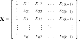 (1.3)
(1.3)
with a leading column of  s (e.g. there are
  explanatory variables here) to estimate a constant (the predicted value of
  when all the values of the explanatory variables are set to zero,
  ). The vector
  contains the targets of regression analysis, which tell us how important or unimportant each associated explanatory variable is in this particular context:
 (1.4)
(1.4)
The vector  contains values of the observed residuals (disturbances, errors) in a column vector:
 (1.5)
(1.5)
Without such matrix notation, statistical regression models are very awkward to describe in formal terms. The simplicity of (1.1) belies its immense power and flexibility: it can include interactions, hierarchies (fixed and random effects), time-series components, different measurements of variables, different link functions, and more.
Notice also that we do not use the term “independent variables” here. This is because in the social sciences there is no such thing as a set of independent variables in this context with real data. That term is more appropriate for the physics or chemistry lab where the variables can actually be independent of each other in a way that is impossible when studying humans. Note that “covariate” is an acceptable term but slightly less informative than “explanatory variable.”
We also want to distinguish between  , the true but unknown value of the regression vector, and
  , the estimate of this quantity. Of course, since we are estimating Bayesian models, we will actually produce a distribution for
  , which can be summarized with measures of centrality, dispersion, and quantiles. Since accurately estimating the true distribution of
  is our goal, we will judge the quality of the individual terms in
  by their diffusion: broad posteriors indicate higher uncertainty than narrow posteriors. As discussed in Gill and Bao (Reference Gill and Bao2024), we can also evaluate the evidence of a marginal effect for a given
  in
in  relative to some threshold such as zero. Often we would like to say something like “there is a 0.98 probability that the effect of the explanatory variable
  on the variability of the outcome
  is positive.” Notice that this type of statement cannot be made in the non-Bayesian context.
Note also that all regression specifications are “semi-causal” in that by specifying (1.1) we are making an assertion that the collective evidence in  explains a large part of the variability in
  . The use of “semi” is very important here because a regression expression is not an assertion of causal inference since there are many other variables, measured or unmeasured, that could also cause variability in
  . However, we specify the variables in
  because we do think that they are explainers of the structure observed in
  , not because they are merely correlated. For instance, shoe size may be correlated with income (and it likely is for spurious reasons), but we would not include shoe size as a column of
  because we do not believe that it is an “explainer.”
In Gill and Bao (Reference Gill and Bao2024) we strongly emphasized using computer simulation to produce desired results with simple Bayesian calculations, even when the analytical calculation was available. Here we move to a world where computer simulation is actually required to get such results. We stated earlier that Markov chain Monte Carlo is essential for estimating nuanced Bayesian regression models. These are forms with nonlinear relationships, time series elements, hierarchies, interactions, and more. As such, much of the work here is dedicated to explaining how MCMC works and how to use it effectively with modern software. This emphasis is important because noncareful estimation with MCMC can go badly wrong. Unfortunately there is plenty of printed evidence of this. So, unlike estimating regular generalized linear models (GLMs) in the regression sense with iterative reweighted least squares (a multidimensional mode finder; see Gill and Torres [Reference Gill and Torres2019] for details), the process is not a simple application of canned software. One advantage to the type of software used for MCMC is that it causes the user to think deeply about the structure of the model being specified. However, it is important not to get lost in the mechanical aspects of estimating Bayesian models with MCMC and lose track of the original research objectives.
We focus here on applying MCMC with JAGS (“Just Another Gibbs Sampler” distributed freely by Martyn Plummer) called from R and PyMC (an open-source probabilistic programming library) in Python but there are other alternatives such as STAN, MultiBUGS, TensorFlow Probability, JAX, and more. In our view, JAGS and PyMC offer an optimal balance of flexibility, power, and ease of learning, with syntax closely aligned with mathematical notation, making them ideal for those new to Bayesian methods.” All code and data used throughout this Element are stored in a GitHub repository (https://github.com/jgill22/-Bayesian.Social.Science.Statistics2), and can also be conveniently executed online at a Code Ocean capsule (https://codeocean.com/capsule/0249394). We now turn to a review of Bayesian basics as a refresher.
2 A Review of Bayesian Principles and Inference
This section provides a very brief overview of Bayesian inference purely as a reminder. Readers are assumed to have seen similar discussions along the lines of Gill and Bao (Reference Gill and Bao2024). Fascinating historical accounts can also be found in works such as Dale (Reference Dale2012), McGrayne (Reference McGrayne2011), and Stigler (Reference Stigler1982, Reference Stigler1983). Important theoretical background is provided by Bernardo and Smith (Reference Bernardo and Smith2009), Diaconis and Freedman (Reference Diaconis and Freedman1986, Reference Diaconis and Freedman1998); Gill (Reference Gill2014), Jeffreys (Reference Jeffreys1998), Karni (Reference Karni2007), Robert (Reference Robert2007), and Watanabe (Reference Watanabe2018).
2.1 Basic Bayesian Theory
The Bayesian process of data analysis is characterized by three primary attributes: (1) a willingness to assign prior distributions to unknown parameters, (2) the use of Bayes’ rule to obtain a posterior distribution for unknown parameters and missing data conditioned on observable data, and (3) the description of inferences in probabilistic terms. The core philosophical foundation of Bayesian inference is the consideration of parameters as random quantities. A primary advantage of this approach is that there is no restriction to building complex models with multiple levels and many unknown parameters. Because model assumptions are much more overt in the Bayesian setup, readers can more accurately assess model quality.
The primary goal in the Bayesian approach is to characterize the posterior density of each of the parameters of interest through the computation and the marginalization of the joint posterior distribution of the unknown parameter vector, given the observed data and the model specification,  , for vectors
  and data
  . Here the use of “
  ” is a reminder that this is a posterior (post-data) probability distribution. The posterior distribution of the coefficients of interest is obtained by multiplying the prior by the likelihood function using proportionality:
 (2.1)
(2.1)
meaning that the posterior distribution is a compromise between prior information and data information. The fundamental principle and process of Bayesian inference starts with an unconditional prior distribution,  , that reflects prior belief about the parameters of interest, and multiplies it with the likelihood function,
  , bringing in the data information to produce the posterior distribution,
  . The posterior is now an updated distribution that reflects the most recent knowledge about some phenomenon of interest. Additionally, the result is a distribution, not a point estimate, so uncertainty is built into the results as distributional variability.
This idea of compromise is critical to Bayesian thinking. When there is very reliable prior information and sketchy data information, then we should rely more on the specification of the prior. On the other hand, when there is a large amount of reliable data, then we should favor this type of information over any prior. A key feature of Bayesian inference is that this compromise is mathematically built into the process for any Bayesian result. So we get an important balance based on the amount of contribution from each of the two information sources. In addition, a posterior distribution can be treated as a prior distribution when another set of data is observed, and this process can be repeated as many times as new data arrive to obtain new posteriors that are conditional on all previous sets of observed data, as if they had arrived at the same time. This is a process called “Bayesian updating” or “Bayesian learning.”
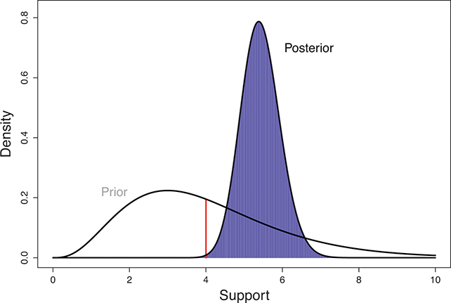
The Bayesian updating process is illustrated in Figure 1 where a gamma distribution prior is applied to a Poisson likelihood function with synthetic data ( ) generated by the R command rpois(20,5) or the Python command np.random.poisson(5,20), for a single parameter
  . This is a conjugate setup, meaning that the form of the prior flows down to the posterior, albeit with different parameterization. Conjugacy is a special, and convenient, case of Bayesian modeling that has simple mathematical properties for determining the posterior distribution. In this case the prior and posterior parameterizations are
using the rate version of the gamma PDF:
 (2.2)
(2.2)
Suppose the threshold at 4 on the  -axis is substantively important. In the prior distribution, 0.566 of the density is to the left of 4, whereas 0.005 of the posterior density is to the left of 4. So, even though there are only 20 data values, the likelihood function changes the prior substantially.

Figure 1 Poisson–Gamma update.
In many Bayesian models, priors themselves have prior parameters (hyperpriors), so there can be additional terms in the product but no substantial increase in complexity:
 (2.3)
(2.3)
where  is a higher-level parametric assignment with prior distribution
  . Proportionality as used in (2.3) is typically employed to simplify the notation, since in the Bayesian setup,
  is observed and therefore is assumed fixed and independent of
  . In addition, Bayesian model specification can be naturally hierarchical, since parameters and hyperparameters can be conduits to additional specifications at group levels.
2.2 Interval Estimation
Highest posterior density (HPD) regions are the Bayesian equivalent of confidence intervals in which the region describes the area over the coefficient’s support with  % of the density with the highest probability. Like frequentist confidence intervals, an HPD region that does not contain zero implies that the coefficient estimate is deemed to be reliable, but instead of being
  % “confident” that the interval covers the true parameter value over multiple replications of the exact same experiment, an HPD interval provides a
  % probability that the true parameter is in the interval. Sometimes HPD regions are relatively wide, indicating that the coefficient varies considerably and is less likely to be reliable, and sometimes these regions are quite narrow, indicating greater certainty about the central location of the parameter. Highest posterior density regions do not have to be contiguous, and contiguous HPDs (no breaks on the
  -axis) are usually called credible intervals.
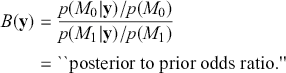
2.3 The Bayes Factor
Formal hypothesis testing can also be easily performed in Bayesian inference. Start with  and
and  representing competing hypotheses about the location of some
  parameter to be estimated. These two statements about
  form a partition of the sample space, meaning that
  , where “
  ” denotes the empty or null set. Now prior probabilities are assigned to each of the two outcomes:
  and
and  . Since the priors are different (but the form of the likelihood function is the same), there are two competing posterior distributions:
  and
and  . We can now define the prior odds,
  , and the posterior odds,
  . This leads to a prior-to-posterior ratio of
  , which is called the Bayes factor, interpreted as odds favoring
  versus
  given the observed data, and it leads naturally to Bayesian hypothesis testing. Another interpretation is that the Bayes factor is the ratio of improvement in odds by accounting for the data.
More formally, start with the two competing models,  and
and  . Specify corresponding parameter priors:
  ,
,  , and model priors:
  and
and  . Note that
 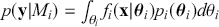 . Therefore:
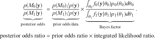 (2.4)
(2.4)
Now rearranging and canceling out  gives:
 (2.5)
(2.5)
The Bayes factor here is analogous to a likelihood ratio test, except that it includes prior information. Also, the tested hypotheses do not need to be “nested” as does the likelihood ratio (one model is a subset of the other). Regretfully, though, there is no distributional test for the Bayes factor. Since a result near one is obviously inconclusive, what we want is a number that is decisively large, like 10 or greater, or decisively small, like 0.1 or less. There are some published thresholds contained in Jeffreys (Reference Jeffreys1998) and Kass and Raftery (Reference Kass and Raftery1995), but they are completely arbitrary.
It is important to know that the Bayes factor as evidence is completely different than using p-values (or similar devices) in non-Bayesian inference. For example, consider testing whether a coin is fair or biased at a specific value:  versus
  . Assign equal priors:
 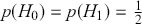 , so that the prior odds ratio is just one, which is commonly done. We flip the coin 10 times and get 7 heads, which is exactly at the alternative hypothesis. The Bayes factor between “model 0 supported” and “minimal evidence against model 0” is calculated by
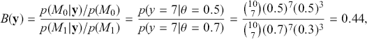
which provides no strong evidence for either hypothesis. Now calculate the p-value in the standard way:
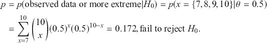
Notice that the manner in which we make these conclusions is very different. The surprising result is that we cannot reject  with the p-value as evidence even though the data landed right on the alternative of
  . This is because the two hypotheses are relatively close and p-values are poor tools for asserting scientific evidence. Bayes factors are very compelling because they provide a direct way to compare competing hypotheses that include both prior and data information, but there are some shortcomings. First, they are known to be sensitive to the choice of priors, although an overwhelming number of authors set the prior probabilities to 0.5 each. Second, there is no ability to have directional hypotheses in the conventional sense. However, direction can be built into the hypothesis structure by specifying regions such as
  versus
  . Finally, improper priors (those that do not sum or integrate to a finite value) do not work because the infinity values do not cancel out in the ratio, although there are several rather tortured work-arounds; see Gill (Reference Gill2014), chapter 6.
2.4 Using Simulation
The challenge before us now is to use these Bayesian principles to develop regression-style specification of interest to social scientists. However, many of the important and popular forms require Markov chain Monte Carlo (MCMC) so that the computer performs the difficult or impossible tasks for us in estimating these forms and getting marginal posterior distributions for each of the unknown parameters. One major impediment to wide usage of Bayesian regression specifications is the hurdle of learning MCMC. We break it down into three stages here: (1) understanding the general principle of Monte Carlo methods for making the computer do a lot of repetitive tasks, (2) defining what a Markov chain does mathematically in an accessible way, and (3) combining these two principles to produce a powerful tool that lets Bayesians model nearly anything. Our objective in the next three sections is to demystify MCMC tools and make them widely usable to a large class of researchers. We do this by introducing Monte Carlo simulation in the next section, then in Section 4 we provide a gentle introduction to the mathematics of Markov chains and then combine these principles to produce the powerful MCMC estimation engine in Section 5.
3 Monte Carlo Tools for Computational Power
This section introduces Monte Carlo Methods in statistics. This is a very important component to modern practice that exploits a computer’s ability to do a large number of mundane tasks. Such simulation work in applied and research statistics replaces analytical work with repetitious, low-level effort by the computer. So if a distribution is difficult or impossible to manipulate analytically, then it is often possible to create a set of simulated values that share the same distributional properties, and describe the posterior by using empirical summaries of these simulated values. This process was termed Monte Carlo simulation by Von Neumann and Ulam in the 1950s (although some accounts attribute the naming to Metropolis too) because it uses randomly generated values to perform calculations of interest, reminiscent of expected value calculations in gambling.
3.1 Random Number Generation with Uses
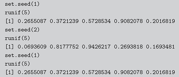
Surprisingly, all random number generation starts with producing  continuous uniform random variables within computer algorithms. Then there is a large set of transformations that provide any distributional form of interest. These uniform random numbers are actually not random at all. They are pseudo-random numbers that are produced deterministically by the computer with a defined period before repeating the sequence identically. Fortunately, due to work mostly done in the 1980s, the length of this period is so large that we do not have to care. We can generate different sequences by setting a “seed” to start a new process. This is illustrated in the following code boxes in R and Python where we set this random seed before generating five
  random numbers, change the seed to produce a different set, and then change the seed back to get the original set again.

Code 1.01
 set.seed(1)
 runif(5)
 [1] 0.2655087 0.3721239 0.5728534 0.9082078 0.2016819
 set.seed(2)
 runif(5)
 [1] 0.0693609 0.8177752 0.9426217 0.2693818 0.1693481
 set.seed(1)
 runif(5)
 [1] 0.2655087 0.3721239 0.5728534 0.9082078 0.2016819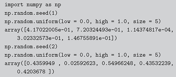
Code 1.02
 import numpy as np
 np.random.seed(1)
 np.random.uniform(low = 0.0, high = 1.0, size = 5)
 array([4.17022005e-01, 7.20324493e-01, 1.14374817e-04,
 3.02332573e-01, 1.46755891e-01])
 np.random.seed(2)
 np.random.uniform(low = 0.0, high = 1.0, size = 5)
 array([0.4359949 , 0.02592623, 0.54966248, 0.43532239,
 0.4203678 ])
The Monte Carlo principle is actually much more general than this, even though generating random numbers according to some distribution is very important. Suppose we could generate random numbers in a way that does work for us, and often you can get the right answer faster with simulation than by analytics. For instance, what is the 90 percent confidence interval for a random variable distributed  ? This is obviously an easy analytical calculation but we can also do this quickly with two lines of code as shown in what follows (one line if we want to be clever). We simply generate 1,000,000 values from the desired normal distribution, sort them, and find the desired interval end-points empirically as if these were actual data. The large number of generated values (it can be larger) assures us a high level of accuracy.
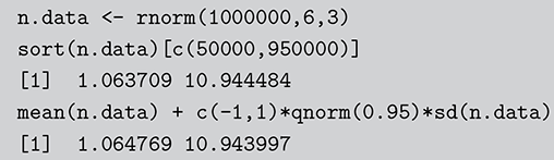
Code 1.03
 n.data <- rnorm(1000000,6,3)
 sort(n.data)[c(50000,950000)]
 [1] 1.063709 10.944484
 mean(n.data) + c(-1,1)*qnorm(0.95)*sd(n.data)
 [1] 1.064769 10.943997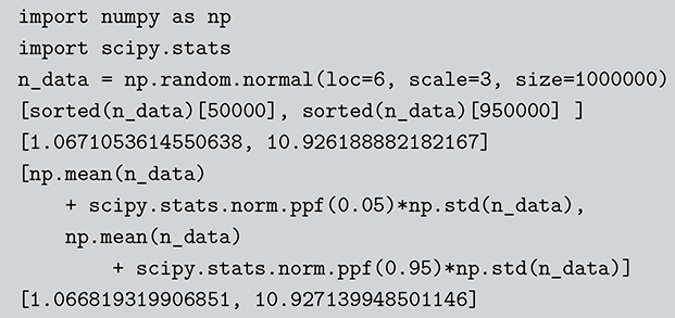
Code 1.04
 import numpy as np
 import scipy.stats
 n_data = np.random.normal(loc=6, scale=3, size=1000000)
 [sorted(n_data)[50000], sorted(n_data)[950000] ]
 [1.0671053614550638, 10.926188882182167]
 [np.mean(n_data)
 + scipy.stats.norm.ppf(0.05)*np.std(n_data),
 np.mean(n_data)
 + scipy.stats.norm.ppf(0.95)*np.std(n_data)]
 [1.066819319906851, 10.927139948501146]
Here R and Python have slightly different answers because the default random number generators are different. Notice also that the two methods also have slightly different answers and this is due to rounding in the different calculations. There is also an error term introduced by using Monte Carlo methods instead of an analytical calculation: simulation error. The good news, however, is that this type of error decreases at a rate of  , where
  is the number of simulated values used. This means that the user controls the simulation error and the only cost is additional user time on increasingly fast computers.
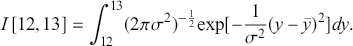
3.2 Basic Monte Carlo Integration
Another use of Monte Carlo simulation is doing integral calculus that is hard or impossible analytically. Suppose  is a function that is difficult to integrate over a specific range but we can draw values from this form. For example, the expected value of
  distributed
  restricted to being between
  and
and  is given by the integral:
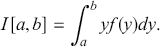 (3.1)
(3.1)
To get this integral by simulation, first generate a large number ( ) of simulated values of
  from
from  . Then we discard any values below
  and above
  to get the sample
  (e.g. left after truncation). The estimate of the integral is merely
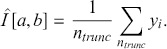 (3.2)
(3.2)
So we substitute a mean of the empirical sample for the analytical integral calculation. From the Strong Law of Large Numbers, the calculation of  converges with probability one to the actual true answer. As in the preceding example the simulation error of
  goes to zero proportional to
  . In this case the expression of the variance of the simulation estimate is
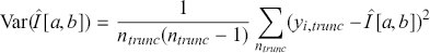 (3.3)
(3.3)
Note that the researcher fully controls the simulation size,  , and therefore the simulation accuracy of the estimate.
As a specific example, suppose we want to integrate a  over the range
  :
:
This is easily calculated by the following:
The calculation is given in the following R and Python code boxes.
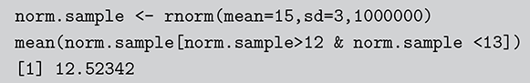
Code 1.05
 norm.sample <- rnorm(mean=15,sd=3,1000000)
 mean(norm.sample[norm.sample>12 & norm.sample <13])
 [1] 12.52342
Code 1.06
 norm_sample = rng.normal(loc=15, scale=3, size=1000000)
 np.mean(norm_sample[(norm_sample >= 12)
 & (norm_sample <= 13)])
 12.524258697969533
In a Bayesian context using 3.1 we can replace arbitrary  with a posterior statement
  and
and  in the preceding with
  . So
. So  is the posterior expectation of
  , given by:
 (3.4)
(3.4)
We can see here that if it is possible to generate values from  , then we can calculate this expected value or any other related statistic. This is actually the last step of the MCMC process, which we will see in Section 4.2 on Markov Chain Theory.
3.3 Rejection Sampling
Suppose that we lack the ability to produce samples from some known distribution but we still have a difficult analytical problem that suggests Monte Carlo simulation. In some circumstances we can then use rejection sampling to integrate as done earlier. Rejection sampling is actually used in two primary contexts: obtaining dimensional integral quantities, and generating random variables. In addition, rejection sampling can be particularly useful in determining the normalizing factor for nonnormalized posterior distributions. The very general steps are as follows:
find some other distribution that is convenient to sample from, where it must enclose the target distribution.
compare generated values with the target distribution and decide which values to keep and which to reject.
the integral of interest is the normalized ratio of these values.
The easier case is when the target function has bounded support: a defined, noninfinite support of some PDF or other function. Consider a function of interest  such that it can be evaluated for any value over the support of
  :
:  . We want to put a “box” around the function and we have the two sides of the rectangle from
  and
and  . Since our interest is almost always centered on probability functions, the bottom of the box is the x-axis at zero. To determine the top of the box we can use various mathematical tools like analytical root finding, numerical techniques such as gridding, Newton–Raphson, EM, etc. to find
  . So we have defined a rectangle that bounds all possible values for the pair
  . Other geometric forms work too. The objective is now to sample the two-dimensional random variable in this rectangle by independently sampling uniformly over
  and
and  then pairing to produce a point in 2-space. Finally all we have to do is count the proportion of points that fall inside the region of interest. The value of the integral, which is the area under the curve, is the ratio of the generated points under the curve compared to the total number of points scaled by the known size of the box:

As with all Monte Carlo simulations, the error rate goes to zero proportional to  .
.
A curve of interest is plotted in Figure 2 with 500 points generated uniform randomly inside the rectangle. Normally many more points are generated to ensure good Monte Carlo accuracy (low error), but the number is limited here for graphical purposes. There are 99 accepted points (marked with “+”) under the curve, and 401 rejected points (marked with “x”) above the curve. and 401 rejected red points above the curve. The rectangle has sides of length  by construction. So the area under the curve (the integral) is calculated by:
This was straightforward because we were able to easily put a box around the function of interest. The key feature of this example is that while we could not integrate the function, we were able to insert values of  and get values of
  .
.
Figure 2 Example of Rejection Sampling
A more difficult version of this problem is when the target function,  , has unbounded support, like say a gamma distribution with support
  . In this case we need to identify a majorizing function that fully envelopes the target in a way that a rectangle cannot, and can still have values drawn from. The rectangle was convenient because the size is simply height times width. Typically a chosen majorizing function,
  , is a PDF chosen such that
  for the full support of
  . To make sure that this property holds, it is always necessary to multiply the candidate generating function by a constant:
  . The steps are slightly different since we do not have the same height on the y-axis over the support. The steps are as follows:
uniformly randomly generate many points on the support of
 (x-axis), .
for all
, points calculate .for all
, generate a unique value, .accept points if
.otherwise reject.


The setup is critical here. If the majorizing function is highly dissimilar than the target function, then a lot of values will be rejected and the algorithm will be inefficient. Rejection sampling is actually a fundamental part of one of the two important MCMC procedures.
Now we can state the Fundamental Principle of Monte Carlo Simulation. If we have many draws from a distribution of interest (or other functional forms), then we can use these draws to calculate any value of interest, with a known error rate. A key word in that definition is “any,” meaning that we can empirically calculate means, variances, intervals, quantiles, higher-order moments, and more. Thus, this process replaces analytical work for hard problems but does not deter us from getting values or summaries of interest.
Monte Carlo analysis has been around since the infancy of programmable computers in the early 1950s. Physicists such as Ulam, Von Neumann, Metropolis, and Teller were exploring subatomic properties developing nuclear weapons, but in some cases could not design the relevant physical experiments. So they turned to this new device called the computer and simulated the properties of interest. One important paper that is still cited and relevant to us in Section 5, is Metropolis et al. (Reference Metropolis, Rosenbluth, Rosenbluth, Teller and Teller1953). In this case the authors were interested in the paths of particles inside a box when the box is being squeezed down to a singularity.
General statistical interest in Monte Carlo methods in statistics started roughly in the 1980s when researchers were first having personal computers on their office desk. As these computers became more common and more powerful, Monte Carlo simulation became much more common because it made difficult calculations easier. If one were to look into the office of a research statistician in the 1970s, she would almost certainly be deriving properties analytically. Today, that same person is doing that same work on the same sorts of problems but mainly with various simulation tools. We now turn to the theoretical basics of Markov chains.
4 A Simple Introduction to the Mathematics of Markov Chains
4.1 A Modeling Exercise
As a motivating example for our efforts to learn MCMC for Bayesian estimation, consider a dataset used in Gill and Casella (2009) looking at a puzzle in bureaucratic politics. These data contain every federal political appointee to full-time positions requiring Senate confirmation from November 1964 through December 1984 (collected by Mackenzie and Light, ICPSR Study Number 8458, Spring 1987). Their survey queries various aspects of the Senate confirmation process, acclamation to running an agency or program, and relationships with other functions of government. But these researchers needed to preserve anonymity of the interviewed so they embargoed some variables and randomly sampled 1,500 down to 512. This provides some methodological challenges, but we will ignore them here. So every respondent in the data ran a US federal agency or some major component of it. The puzzle is that even though all of them have to nominated by the president, underwent grilling on Capitol Hill, moved to an expensive real estate market, hired a lawyer or advisor for the process, often left a high-paying corporate position, and uprooted a family,  they stayed in the position on average for only about two years. Fortunately, there is a convenient outcome variable that may explain this phenomenon: stress, which can be considered as a surrogate measure for self-perceived effectiveness and job-satisfaction recorded as a five-point scale from “not stressful at all” to “very stressful.” The emphasis in this Element is on Bayesian regression models, so consider the explanatory variables in Table 1.
| Variable | Description |
|---|---|
| Government Experience | a dichotomous measure of previous government employment |
| Ideology | a seven point ideology scale in the Republican direction to the right |
| Committee Relationship | a self-assessment of the relationship with the primary Congressional committee |
| Career.Exec-Compet | an assessment of the competence of direct reports |
| Career.Exec-Liaison/Bur | an assessment of the effectiveness of underlings to liaise with other agencies |
| Career.Exec-Liaison/Cong | an assessment of the effectiveness of underlings to liaise with Congress |
| Career.Exec-Day2day | an assessment of direct reports to handle routine business |
| Career.Exec-Diff | an assessment of direct reports helpfulness |
| Confirmation Preparation | did the executive need preparation from the administration before testifying |
| Hours/Week | how many hours per week does the executive work on average |
| President Orientation | did the executive need policy briefings on the presidents priorities |
This is a rich dataset and there are many other variables to explore. Given that the chosen outcome variable is an ordinal scale, an “ordered choice model” makes sense. This name actually comes from economics, but applies to any regression outcome that is ordinal (i.e. not necessarily a “choice”). The model starts with assuming that there is a latent dimension underlying these observed ordinal categories. In a perfect world we could put some sort of a meter up to people’s heads and measure the exact level of stress in that person. In reality we have to live with some ordinal survey response, with five categories in this case. However, the model specification first assumes that we have the exact level measurement on the utility metric and then assumes that there are categories imposed on this latent scale from the survey wording. The setup looks like this:

Now the vector of (unseen) utilities across individuals in the sample,  , is determined by a linear additive specification of explanatory variables:
  as if we could see the latent dimension for real, where
  does not depend on the
  cutpoints between categories, and the residuals have some distribution that we have not assigned yet,
  , stated in cumulative distribution terms (CDF). These cutpoints between categories also need to be estimated on this latent scale and are sometimes called “fences” or “thresholds.” The key to understanding this model is to see that it initially assumes we know something that we cannot know: the true latent dimension. Another key point to note is that the model is initially given all in cumulative terms. This means that the probability that individual
  in the sample is observed to be in category
  or lower is:
 (4.1)
(4.1)
which is differently signed than the popular MASS package in R, which states  from the help page. It is very irritating that the sign in front of
  varies by author and software, but we just have to live with that. One convenient way to figure out which sign is being used is to check the effect of an “obvious” explanatory variable. So, for example, in voting models we know that people get more conservative as they get older and richer. This is not a perfect recommendation but it helps to make up for technical omissions by some authors. Now specifying a logistic distributional assumption on the residuals produces a logistic cumulative specification for the whole sample:
 (4.2)
(4.2)
However, a probit (cumulative normal) distribution is another popular choice.
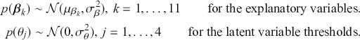
Of course, this work is about Bayesian specifications for social science models so we need to specify prior distributions for the  parameters. However, this differs from simpler regression models in that we also need to specify prior distributions for the
  cutpoint parameter as well. So, let’s specify the most simple possible and nearly conjugate forms as possible to keep this extended example as direct as possible:
Here is the problem; all this produces a posterior distribution according to
 (4.3)
(4.3)
where  denotes the cumulative density function (CDF) of the logistic distribution, meaning this is actually a simplified version. What is this? It is a big joint posterior probability distribution with 16 dimensions, from the 11 explanatory variable parameters, the 4 threshold parameters, and the density (probability) over them. While this form tells us everything we need to know about the joint distribution of the model parameters, we need to marginalize (integrate) it for every one of these parameters to create an informative regression table. This may be very difficult or even impossible. We do not know. But wait! This is a standard model in the toolbox of most practicing quantitative social scientists and we just showed that specifying the most simple Bayesian version of this model leads to an intractable mathematical problem. This example is provided because it highlights the key problem of practicing Bayesian modelers prior to 1990. This was an insurmountable task for twentieth-century Bayesians that was solved in 1990. It turns out that there was a tool hiding in statistical physics and image restoration that completely solved this issue. Employing Markov chain Monte Carlo (Gibbs sampling in this case) allows us to report the standard regression table output in Table 2. Here we see a mixture of results quality. Two reliable effects are interesting: pre-hearing confirmation preparation lowers stress and greater work hours increase stress. Of course, these are nuanced qualitative effects that warrant further investigation.
Table 2Long description
The table includes means, standard errors, and 95% highest posterior density (HPD) intervals for explanatory variables and threshold intercepts. HPD intervals are displayed as horizontal lines with a dashed vertical line at zero for reference. Several intervals lie entirely to one side of zero (e.g., *Career.Exec-Compet*, *Career.Exec-Liaison/Bur*, and *President Orientation*), indicating stronger evidence for nonzero effects. The estimated standard deviation of the latent scale is reported as 6.04 (SD = 1.20).
We know that scientific advances do not proceed in a linear fashion (Kuhn, Reference Kuhn1997), and this is a classic example of that. A review paper in 1990 (Gelfand & Smith, Reference Gelfand and Smith1990) changed all of this story. Now we turn our attention to this technology and the basic theory to understand it, starting with the mathematics of Markov chains.
4.2 Markov Chain Theory
The first step in this process is to understand some basic random variable definitions that occur over time. This is a case where the mathematical language does not reflect the simplicity of the principles, so it is important not to be intimidated by the vocabulary.
A stochastic process is a consecutive set of random quantities,  s, defined on some known state space,
  , indexed so that the order is known:
  . So
. So  is a generic random variable in the standard statistical sense except that it is observed in a serial manner rather than just all at once in a standard sampling scheme. Here
  just indexes the time of arrival and typically, but not necessarily,
  is the set of positive integers implying consecutive, even-spaced time intervals:
  . This state space is either discrete or continuous depending on how the variable of interest is measured. So, while the term “stochastic process” sounds very mathematical and intimidating it is really just the simple idea that random variables can have scheduled arrival times.
A Markov chain is a stochastic process with the property that any specified state in the series,  , is dependent only the previous value of the chain,
  . Therefore, values are conditionally independent of all other previous values:
  . More formally:
 (4.4)
(4.4)
where this is the probability that  lands in some region
  , which is any identified subset (an event or range of events) on the complete state space defined by
  . We will use this
  notation extensively. Colloquially we can say:
“A Markov chain wanders around the state space caring only about where it is at the moment in making decisions about where to move in the next step.”
Anyone who has ever owned a house cat or been around them much will certainly feel that cats have a very Markovian quality to their behavior. Again, this is a simple idea that unfortunately gets wrapped up in intimidating mathematical language. Necessarily Markov chains are based on a probabilistic process, a “kernel,” that makes a decision about the next draw of  at time
  based only on the current existing draw of
  at time
  . This leads to the standard analogy that the Markov chain is traveling through the state space defined by the support
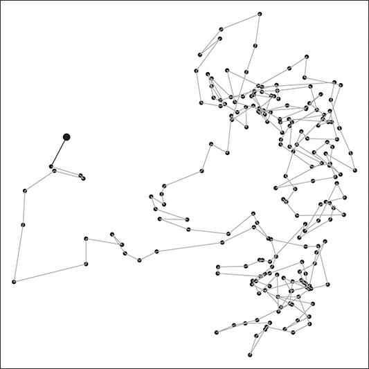
  . So we think of a serial path of the chain like an ant wandering around some topology on the ground. Consider Figure 3 where a 2-dimensional Markov chain is started at the point indicated by a larger dot (all Markov chains need an arbitrary starting point in the sample space), and the first step indicated by the bold black line segment segment. In this case we would call this a random walk Markov chain because we have not imposed any conditions on its behavior other than a random normal draw added to the current position.

Figure 3 Sample Markov Chain Path
So why is the Markovian property useful? This “short-term” memory property is very handy because when we impose some specific mathematical restrictions on the chain and allow it to explore a specific distributional form, it eventually finds the region of the state space with the highest density, and it will wander around there producing an empirical sample from it in proportion to the probability. If this distribution is the posterior from model, then we can use these “empirical” values as legitimate posterior sample values. Thus, difficult posterior calculations can be done with MCMC by letting the chain wander around “sufficiently long,” thus producing summary statistics from recorded values. For example, if we wanted marginal draws from the big awkward joint distribution in (4.3) then the Markov chain explores the multidimensional state space recording where it has been for us. This means that we can take the empirical values for each dimension (model parameter) and summarize them any way we want.
To clarify this strategy, consider the output of a Markov chain with 5 parameters run for 500,000 iterations. This means that it has visited 500,000 locations in the state space, and each 5-dimensional location is a row of a stored matrix. To get the marginal distribution analytically by contrast for just  , we would have to perform the integration in four steps:
 (4.5)
(4.5)
That’s a lot of work! And that’s for one of the dimensions; it needs to be done for all 5 of them. Recall from the structure of the joint distribution in (4.3) that this can be really hard or even impossible for humans with some model specifications. However, once we have run the Markov chain sufficiently long (more on this shortly) and stored the values in matrix form, then we get an empirical distribution for each of the parameters simply by looking down the columns. For instance, rather than do the integration process in (4.5), we would just pull out the values in column one to produce a vector of draws for the first parameter only. Doing the integration process gives an exact marginal distribution in mathematical terms,  . But wait! If we have half-a-million draws from this marginal distribution, then we actually have all of the information we need to know for scientific purposes. That is, we can take the mean and standard deviation of the vector to produce the information needed for a regression table. We can also calculate any other desired statistic or summary: quantiles, different measures of centrality and variance, probabilities over ranges, HPD intervals, and so on. Furthermore, given the Law of Large Numbers we know that we are very nearly precisely correct, given a very big number of draws like 500,000.
How does the Markov chain decide to move? The Markov chain moves based on a probability statement so we need to define how probability enters the decision. First, define the transition kernel,  , as a very general, and for the moment unspecific, mechanism for describing the probability of moving to some other specified state based on the current chain location. Here
  is a defined probability measure for all
  points in the state space to the set (subspace)
  . Therefore
  maps potential transition events to their probability of occurrence. Note that, in the current discussion,
  is a multidimensional point in the sample space and not a coefficient to be estimated. This is slightly confusing given the preceding discussion, but this notation is consistent with the literature.
Let us start with a simple discrete form of a two-dimensional state space,  , with 64
  locations: the chess board. Discrete state spaces in this discussion are much easier to conceptualize so we will restrict ourselves to this form for now. It is also easy with this example to define various
  subspaces, like, say, the four squares in the top right-hand side of this chess board. The most flexible and powerful piece in chess is the Queen who can move any distance on the board vertically, horizontally, and diagonally. Now imagine a Super-Queen who can move from any square to any other square on the chessboard in one move, arbitrarily for from
  to
to  , where the transition kernel is uniform selection of any of the 64 squares. Thus we have 64 moves from some
  to another
  , including moving to where we already are:
  . The latter scenario is included because the current location is always a valid destination for a Markov chain.
When the state space is discrete,  is a matrix mapping for
  discrete elements in
  , where each cell defines the probability of a state transition from the first term to all possible states. So for a rectangular 2-dimensional state space like the chess board (
 ), the transition matrix giving the probabilities of moving from any square to any other square for our Super-Queen is:
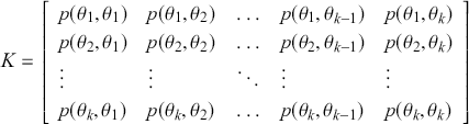
where the row indicates where the chain is at this period. Thus the first row gives the 64 probabilities of starting at  (say the top leftmost corner if we are mapping the chess board like reading a paragraph) to all of the 64 possible destinations starting with
  for returning to the current location using up a unit of time index, and proceeding to
  for moving from the top left corner to the bottom right corner. It is important that each matrix row is a well-behaved probability function,
  in the sense of the Kolmogorov Axioms. Rows of
  sum to one and define a conditional probability mass function (PMF) since they are all specified for the same starting value as the condition and cover each possible destination in the state space: for row
  :
:  . As a side note for now, when the state space is continuous, then
  is a conditional PDF:
  .
.
Consider a very simple mathematical example to get us started. Define a two-dimensional state space: a discrete vote choice between two political parties, a commercial purchase decision between two brands, a choice by a nation to go to war with another nation, and so on. In this setup, voters, consumers, predators, viruses, and so on. who normally select  have a 70% chance of continuing to do so, and voters/consumers/predators/viruses/and so on who normally select
  have an 80% chance of continuing to do so. This provides the transition matrix
  :
:
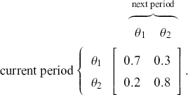
As a running hypothetical case, suppose we are doing market research for a major toothpaste brand and  designates a purchase of Crest, and
  designates a purchase of Colgate. So from the preceding transition matrix, in any given time period, 70% of the Crest buyers stay loyal whereas 80% of the Colgate buyers remain loyal. This is just a mapping from one time period to the next since it defines a Markovian process where the past before that does not matter. All Markov chains require a starting point, in this context set by a human to
meaning that we initially recruit a sample that is one-half Crest buyers and one-half Colgate buyers. To go from this initial state to the first state, we simply postmultiply the starting state by the transition matrix:
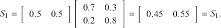
So, observing our sample’s purchase at time period  , we see that 45% bought Crest and 55% bought Colgate. This series of observed purchases continues multiplicatively as long as we want to study our sample:
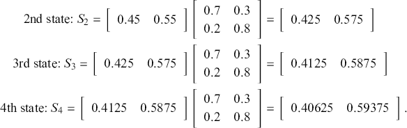
If we continued this process a few more times, the resulting state of  would emerge (try it!) and would never change no matter how many times we performed this operation. This is called the steady state, the stationary distribution, or the ergodic state (the latter for reasons that we will see later on page 31). Markov chains are not guaranteed to have this property and those that do not are called transient Markov chains.
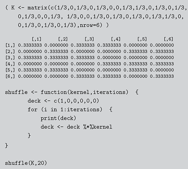
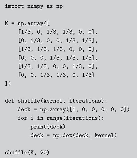
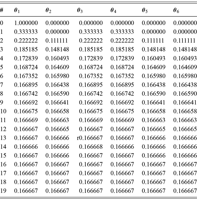
In this section we describe another simple discrete Markov chain simplified from Bayer and Diaconis (Reference Bayer and Diaconis1992), and also described in Gill (Reference Gill2014). Suppose we have the following algorithm for shuffling a deck of cards: take the top card from the deck and with equal probability place it somewhere in the deck, then repeat many times. The objective (stationary distribution) is a uniformly random distribution in the deck: for any given order to the stack, the probability of any one card occupying any one position is 1/52. Is this a stochastic process? Sure, there is a set of discrete outcomes which are the ordering of the deck that change with each step and have a state space that is  big. Is this a Markov chain? Yes, clearly, because if we want to know the probability that the deck is in some specific ordering after the next step we only need to know the current status of the deck to compute the probabilities of the 52 possible arrangements at the next state. These are presumably all
  if we adhere to the condition of uniform random replacement presented earlier. So the previous states of the deck do not help us in any way. As long as we know the current state of the deck we have all the information required to use the transition kernel to move. What is the limiting distribution? For this, we will use simulation as a convenience as noted many times here.
For simplicity and without loss of generality we will use a deck with only  cards. This is the same problem as using
  cards but is a lot easier to describe and visualize. With three numbered cards we have a sample space of size
  given by
  . Given the uniformly random replacement construction of the algorithm, the transition kernel matrix is:
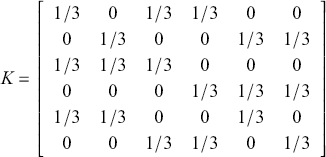
We will use the starting point  , which is analogous to a new deck of cards after one takes off the plastic wrapping and discarding the jokers. We start by defining this matrix and a function to implement the shuffling in both R and Python.

Code 1.07
 ( K <- matrix(c(1/3,0,1/3,0,1/3,0,0,1/3,1/3,0,1/3,0,1/3,
 0,1/3,0,0,1/3, 1/3,0,0,1/3,0,1/3,0,1/3,0,1/3,1/3,0,
 0,1/3,0,1/3,0,1/3),nrow=6) )
 [,1] [,2] [,3] [,4] [,5] [,6]
 [1,] 0.3333333 0.0000000 0.3333333 0.3333333 0.0000000 0.0000000
 [2,] 0.0000000 0.3333333 0.0000000 0.0000000 0.3333333 0.3333333
 [3,] 0.3333333 0.3333333 0.3333333 0.0000000 0.0000000 0.0000000
 [4,] 0.0000000 0.0000000 0.0000000 0.3333333 0.3333333 0.3333333
 [5,] 0.3333333 0.3333333 0.0000000 0.0000000 0.3333333 0.0000000
 [6,] 0.0000000 0.0000000 0.3333333 0.3333333 0.0000000 0.3333333
 shuffle <- function(kernel,iterations) {
 deck <- c(1,0,0,0,0,0)
 for (i in 1:iterations) {
 print(deck)
 deck <- deck %*%kernel
 }
 }
 shuffle(K,20)
Code 1.08
 import numpy as np
 K = np.array([
 [1/3, 0, 1/3, 1/3, 0, 0],
 [0, 1/3, 0, 0, 1/3, 1/3],
 [1/3, 1/3, 1/3, 0, 0, 0],
 [0, 0, 0, 1/3, 1/3, 1/3],
 [1/3, 1/3, 0, 0, 1/3, 0],
 [0, 0, 1/3, 1/3, 0, 1/3]
 ])
 def shuffle(kernel, iterations):
 deck = np.array([1, 0, 0, 0, 0, 0])
 for i in range(iterations):
 print(deck)
 deck = np.dot(deck, kernel)
 shuffle(K, 20)
Running this in either language provides the output probabilities at times in Table 3. Since each value is the probability of being in one of the six states at the time indicated by the iteration number it is easy to see that this Markov chain reaches its stationary distribution at about  (subject to a little rounding of course). It also shows that the shuffling algorithm provides a fully shuffled deck since every one of the six outcomes has equal probability at this point.
| # |  |  |  |  |  |  |
|---|---|---|---|---|---|---|
| 0 | 1.000000 | 0.000000 | 0.000000 | 0.000000 | 0.000000 | 0.000000 |
| 1 | 0.333333 | 0.000000 | 0.333333 | 0.333333 | 0.000000 | 0.000000 |
| 2 | 0.222222 | 0.111111 | 0.222222 | 0.222222 | 0.111111 | 0.111111 |
| 3 | 0.185185 | 0.148148 | 0.185185 | 0.185185 | 0.148148 | 0.148148 |
| 4 | 0.172839 | 0.160493 | 0.172839 | 0.172839 | 0.160493 | 0.160493 |
| 5 | 0.168724 | 0.164609 | 0.168724 | 0.168724 | 0.164609 | 0.164609 |
| 6 | 0.167352 | 0.165980 | 0.167352 | 0.167352 | 0.165980 | 0.165980 |
| 7 | 0.166895 | 0.166438 | 0.166895 | 0.166895 | 0.166438 | 0.166438 |
| 8 | 0.166742 | 0.166590 | 0.166742 | 0.166742 | 0.166590 | 0.166590 |
| 9 | 0.166692 | 0.166641 | 0.166692 | 0.166692 | 0.166641 | 0.166641 |
| 10 | 0.166675 | 0.166658 | 0.166675 | 0.166675 | 0.166658 | 0.166658 |
| 11 | 0.166669 | 0.166663 | 0.166669 | 0.166669 | 0.166663 | 0.166663 |
| 12 | 0.166667 | 0.166665 | 0.166667 | 0.166667 | 0.166665 | 0.166665 |
| 13 | 0.166667 | 0.166666 | r0.166667 | 0.166667 | 0.166666 | 0.166666 |
| 14 | 0.166666 | 0.166666 | 0.166668 | 0.166666 | 0.166666 | 0.166666 |
| 15 | 0.166667 | 0.166666 | 0.166667 | 0.166667 | 0.166666 | 0.166666 |
| 16 | 0.166667 | 0.166667 | 0.166667 | 0.166667 | 0.166667 | 0.166667 |
| 17 | 0.166667 | 0.166667 | 0.166667 | 0.166667 | 0.166667 | 0.166667 |
| 18 | 0.166667 | 0.166667 | 0.166667 | 0.166667 | 0.166667 | 0.166667 |
| 19 | 0.166667 | 0.166667 | 0.166667 | 0.166667 | 0.166667 | 0.166667 |
This example also highlights a very big and important point about Markov chains. The numbers in Table 3 after convergence are marginal probabilities of being in any given state in an arbitrary distant time and for this ergodic Markov chain they will never change. But wait! The Markovian process is a process that produces values at the next iteration conditional on the value at the current iteration. “Conditional” is the operative word here and this is how all Markov chains work. So the contrast is between the conditional distribution that produces the next serially dependent value versus the unconditional future probabilities. Thinking about this another way, in the transition kernel the probability of being at  and moving to
  is zero (we cannot go from
  to
to  in one step), but in the stationary state for some large
  the probability of being in any state is
  because we do not stipulate the state at time
  .
.
Now formalize the idea of the marginal distribution of the chain from applying the transition kernel at some distant time point  giving marginal probabilities that do not change if the chain has reached its stationary distribution. Because this probability structure does not change anymore, we can simply label it as
  . Since time point
  is far from the starting point at time point
  , then we know that
  has been applied many times.
Now we need a set of conditions that assure us that a given Markov chain will eventually reach its stationary distribution, where the marginal distribution is constant and permanent. These mostly have fancy sounding mathematical names and our experience in teaching shows that they can be a little off-putting, but they are in fact fairly direct concepts. Each of these important terms is in bold for later reference.
A Markov chain is said to be homogeneous at step  if the transition probabilities at this step do not depend on the value of
  . More colloquially, elderly Markov chains behave exactly the same as young Markov chains. Now with non-homogeneous Markov chains the transition matrix is not constant but a function of time. This type are useful for modeling probabilistic decay processes, but not for our purposes here.
Recall that Markov chains operate on states, which are subspaces of the state space,  , as in our example of subspaces on of the chess board. These can be individual discrete units or collections of them. The specific state is absorbing if, once the chain enters this state, it cannot leave:
  . The state is transient if the probability of the chain not returning to this state is nonzero:
 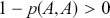 , meaning that there is a finite number of visits in infinite time for the chain. State
  is closed to state
  if a Markov chain on
  cannot reach
  :
:  . State
  is closed in the general sense if it is absorbing.
The state  is irreducible if for all substates
  and
and  in this state, the two substates “communicate,” meaning that every reached point or collection of points (necessarily a subspace in the continuous case) can be reached from every other reached point or collection of points:
So being in any one part of  does not prevent the Markov chain from reaching any other part of
  .
.
The next definition is a “collector” term that combines some of these properties. If a state is (1) closed, (2) discrete, or continuous but finitely bounded, and (3) irreducible, then this state and all subspaces within this subspace are called recurrent. Markov chains operating on recurrent state spaces are labeled as recurrent themselves. A formal definition is:
An irreducible Markov chain is termed recurrent with regard to a given state,  , which is a defined collection of points or bounded area (required for the bounded-continuous case), if the probability that the chain occupies
  infinitely often over unbounded time is nonzero.
Less formally: (1) a recurrent Markov chain run for an infinite amount of time moves into a recurrent state, (2) stays there forever, and (3) visits every subspace an infinite number of times in the limit. This sounds like an odd treatment of infinity, but mathematicians remind us that there are different “flavors” of infinity so it works. Also, a Markov chain is positive recurrent if the mean time to return to  is bounded, Otherwise it is called null recurrent. Additionally, recurrence is an absolute condition in that irreducible chains are either recurrent or transient. For continuous state spaces that are unbounded, like, say, the support of the normal distribution, there is a stricter variant of recurrence called Harris recurrence where the probability of an infinite number of visits to every possible substate of every possible
  is one.
Recurrence is an abstract mathematical concept, but it helps to visualize the chess board again. Suppose  is the topmost four squares on the right-hand side. If we run the Super-Queen for an infinite number of moves, then it will visit
  an infinite number of times and 1 out of 16 times as well. Now consider a different version of
  : the strip of 8 vertical squares on the far left-hand side. The abstract notion of infinity is odd indeed. If the Super-Queen is run under recurrence for an infinite number of moves, it will visit
 th of the time, which is also infinity. In addition, the union of a set of recurrent states (nonempty, and bounded or countable) or Harris recurrent states is a new state that is closed and also irreducible. So the infinity property and the recurrence associated with it also works for the first two columns on the left-hand side consisting of 16 squares.
Define  as the stationary distribution of the Markov chain for
  on the state space
  . Recall that
  is the probability that the chain will move from
  to
to  at some arbitrary step
  , and
, and  is the corresponding marginal distribution. The stationary distribution satisfies
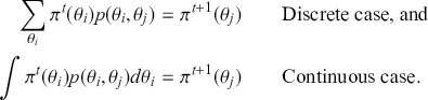
meaning that application of the kernel to the current distribution probabilities returns the same probabilities as seen in the two simple numerical examples presented earlier. This means that the marginal distribution remains fixed when the chain reaches the stationary distribution and we might as well drop the superscript designation for iteration number and just use  . In shorthand:
  . Once the chain reaches its stationary (absorbing) distribution, it stays in this distribution and moves about, or “mixes,” throughout the subspace according to the marginal distribution
  forever. Notice that recurrence gives the range restriction property whereas stationarity gives constancy of the probability structure that dictates movement.
The period of a Markov chain is the length of time required to repeat an identical cycle of chain values. Actually, periodicity is bad and we want an aperiodic Markov chain: the repeating length is the trivial value of one. The problem with periodicity is that it destroys the probabilistic property of the transition kernel. Caveat: all Markov chains run on computers are actually periodic. John Von Neumann’s famous quote on this is: “Anyone who considers arithmetical methods of producing random digits is, of course, in a state of sin” (Von Neumann, Reference Von Neumann1963). Fortunately with modern pseudo-random number generators on computers the period is so large that we need not be concerned as previously noted.
Now we are ready for the big result that all of these conditions have been building up to. If a chain is positive Harris recurrent (unbounded continuous case) or recurrent (discrete/bounded continuous case), and aperiodic, then we call it ergodic. Ergodic Markov chains have the property:
for all  , and
, and  in the subspace. What this means is that once a specified chain has reached its ergodic state, sample values behave as if they were produced independently by the posterior of interest from the model. The Ergodic Theorem is the equivalent of the Strong Law of Large Numbers but for Markov chains, since it states that any specified function of the posterior distribution can be estimated with samples from a Markov chain in its ergodic state because averages of sample values give strongly consistent parameter estimates. Suppose
  are
are  (not necessarily consecutive) values from a Markov chain that has reached its ergodic distribution before time
  , a statistic of interest,
  , can be calculated empirically:
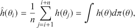 (4.6)
(4.6)
where the summation starts at  since we assume that the Markov chain is in its stationary distribution by time
  , and we consider
  values thereafter. This is the Ergodic Theorem. If
  is the identity function, then this is just the calculation of the expected value of the random variable
  . Notice that once we take this sum we have discarded the order in which the samples arrived. For finite quantities this sum converges almost surely:
 (4.7)
(4.7)
Even though Markov chain values, by their very definition, have serial dependence, the mean of the chain values provides a strongly consistent estimate of the true parameter after convergence. We get an important theoretical result from the Central Limit Theorem. For a given empirical estimator  with bounded limiting variance, we get:
since  is really a mean. The Central Limit Theorem really simply means that nature loves the normal distribution. Here because we are looking at averages taken with large numbers of draws it shows up naturally (pun intended), which is very cool.
What this section provides is the necessary background to understand Markov chains. We will next move on to Markov chain Monte Carlo (MCMC) as a Bayesian estimation procedure. Unlike some standard estimation procedures, either in closed form or through maximization, it is important to understand how Markov chains work since it is easier to apply MCMC incorrectly, which produces misguided results. The mathematics of this section may seem abstract at first, but they really describe a reasonably simple process whereby a stochastic process moves around a state space under a set of very particular rules.
5 Markov Chain Monte Carlo for Estimating Bayesian Models
Section 3 showed how useful the Monte Carlo method can be in solving problems that are annoying or hard for humans but simple for machines to do since they are good at mindless repetition. Then Section 4 provided a brief mathematical explanation of Markov chains. In this section we extend those ideas by putting those two sets of principles together to develop Markov Chain Monte Carlo (MCMC). The key idea is that we set up a Markov chain such that the stationary distribution is the joint posterior distribution and we run the chain for a long period of time, recording where it visits. Since we only consider ergodic Markov chains, we know that the chain will eventually reach this stationary distribution, and since we then run it a long time, we can usually be confident that it will explore the complete state space of interest, thus describing the marginal distributions empirically. So while a single move (there are submoves described in the following discussion) is a move in  dimensional space (
 explanatory variable coefficients and one dimension for probability), we record each move as a discrete vector in this space and thus have a record of each marginal distribution. Consider Figure 4 showing the first two and last two vectors of a run of 1M iterations as rows. Each move of the chain produces a row in this figure, but when we want to summarize a single model coefficient, say
  , we will look down the
  th corresponding column only. So a regression table (or other summary) is built in stages by summarizing each of the
  ’s empirically. This is often done with just a mean and standard deviation calculation for each, but any other summary is available to us since we have something like 1M draws for each variable.
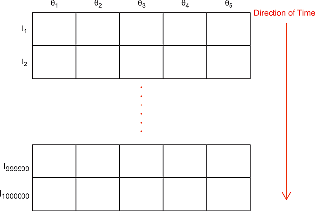
Figure 4 Structure of MCMC Output
Here is the best part, and it’s almost magic except that it is mathematically proven. When the Markov chain is in its stationary (ergodic) distribution, the serially conditional produced draws from the Markovian process “behave” as if they were independent draws from the marginal distributions of interest. This is literally where “Markov chain” meets “Monte Carlo,” meaning that we can treat the draws as if they were from a purely Monte Carlo process even though that is not how a Markov chain produces them mechanically. Cool!
5.1 The Gibbs Sampler
In Section 4 we saw that the mechanism that dictates how a Markov chain moves is a transition kernel ( ). For discrete state spaces, these were shown to be probability matrices and for continuous state spaces, we saw that these were merely probability density functions (PDFs). In general practice, the transition kernel is an algorithm: either the Gibbs sampler or the Metropolis–Hastings rejection procedure, or possibly a hybrid of the two. We now introduce the Gibbs sampler and save the short discussion of Metropolis–Hastings for later.
Gibbs sampling was introduced in a paper by Geman and Geman (Reference Geman and Geman1984) that appeared in the IEEE Transactions on Pattern Analysis and Machine Intelligence, and subsequently went ignored for years (at least by statisticians) until it was discovered by Gelfand and Smith (Reference Gelfand and Smith1990). This is a great example of Stigler’s Law of Eponymy that no discovery in science is ever named for its actual inventor since “Gibbs” comes from the distribution used in the Geman and Geman (Reference Geman and Geman1984) paper not the authors. The Gelfand and Smith publication fundamentally changed statistics and is easily one of the most important contributions to statistics even though it was essentially a review paper. To reflect on the importance, one merely needs to try and read the Geman and Geman paper. So suddenly a huge class of Bayesian models that were difficult or impossible to estimate suddenly became accessible. For a fascinating history of this era see Robert and Casella (Reference Robert and Casella2011).
The Gibbs sampler is a transition kernel created by a series of full conditional distributions that are sampled in cycles. So it is a Markov chain updating scheme based on conditional probability statements where every parameter has its own specification. Suppose that the limiting distribution of interest is  where
where  is a
is a  -length vector of coefficients to estimate. The objective is to produce a Markov chain that cycles through these conditional statements moving toward and then around this distribution. For the moment, consider a joint posterior that we wish to marginalize with
  that is given by
  with data
  and
and  in the regression context. The full algorithm at time
  is given by drawing three random values according to the following expressions:
This is in total a single step of the Gibbs sampler. Clearly this is a Markov chain since the decision to move at time  is only conditional on information at time
  in total. Importantly, notice that each draw is done with the most recent information from the other parameters:
  uses information strictly at time
  since it is drawn first,
  uses information at time
  from
from  but information at time
  for
for  , and
, and  uses information completely from the current step since it is sampled last. Actually, the order of this within-step sampling does not matter, meaning 1,2,3 are in arbitrary order, but it is critical that no matter what the order is, each sub-sampling step is done conditional on the most “modern” version of the other parameters.
Consider data that are normally distributed:  , meaning that we have two parameters to estimate from the joint posterior:
 (5.1)
(5.1)
with researcher-specified normal and gamma priors:
 (5.2)
(5.2)
The full conditional distribution for  is given by:
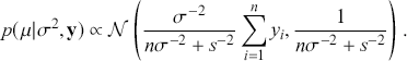 (5.3)
(5.3)
This notation here uses a variance,  , although in Bayesian specifications it is common to use the precision:
  , meaning high variance is low precision. The full conditional distribution for
  is given by the following formula:
 (5.4)
(5.4)
Notice that in both cases the Bayesian principle that posterior information is a compromise between prior information ( ) and data information (
 ) is apparent, and in both cases the data dominate in the limit. So now we have the complete recipe for the Gibbs sampler where we alternate drawing from the full conditional distributions for
  and
and  .
.
As an example, Table 4 contains the percent of the total US vote on “others” (non-Democratic and non-Republican) in the 2020 presidential election by state and the District of Columbia. Some might call these “independents” but there is a literature in political science that finds more nuances. These data are unimodal and almost symmetric and are thus a good candidate for modeling with a normal distribution. Running the Gibbs sampler 20,000 iterations and dispensing with the first 10,000 draws to let the Markov chain reach its stationary distribution (we will discuss “burn-in” in Section 8). This is specified in the following code which returns an empirical mean of 0.347 for  and 0.008 for
  . Interestingly, this model specification for 51 cases is fairly sensitive to the priors selected. This is often not the case with decent sized social science data, so we encourage readers to download the code and data for experiential purposes on this type of situation.
Code 1.09
 elect <- read.table(election.2020.dat",header=TRUE)
 norm.gibbs <- function(y,s2.inv,alpha,beta,n.sims) {
 mcmc.out <- matrix(NA,nrow=n.sims,ncol=2)
 mcmc.out[1,] <- c(0,1)
 n <- length(y)
 for (i in 2:nrow(mcmc.out)) {
 sig2.inv <- mcmc.out[(i-1),2]
 mcmc.out[i,1] <- rnorm(1,
 (sig2.inv/(n*sig2.inv + s2.inv))*sum(y),
 1/(n*sig2.inv + s2.inv))
 mcmc.out[i,2] <- rgamma(1, shape=alpha+n/2,
 rate=beta + 0.5*sum(y-mcmc.out[i,1])^2)
 }
 return(mcmc.out)
 }
 gibbs.vals <- norm.gibbs(elect$Vote.pct,2,2,12,20000)
 apply(gibbs.vals[10001:20000,],2,mean)
Code 1.010
 import pandas as pd
 import numpy as np
 from scipy.stats import norm, gamma
 elect = pd.read_csv("election.2020.csv", header=0)
 def norm_gibbs(y, s2_inv, alpha, beta, n_sims):
 mcmc_out = np.zeros((n_sims, 2))
 mcmc_out[0, :] = [0, 1]
 n = len(y)
 for i in range(1, n_sims):
 sig2_inv = mcmc_out[i-1, 1]
 mu_mean = (sig2_inv / (n * sig2_inv + s2_inv)) *
 np.sum(y)
 mu_var = 1 / (n * sig2_inv + s2_inv)
 mcmc_out[i, 0] = norm.rvs(loc=mu_mean,
 scale=np.sqrt(mu_var))
 shape = alpha + n / 2
 rate = beta + 0.5 * np.sum((y -
 mcmc_out[i, 0])**2)
 mcmc_out[i, 1] = gamma.rvs(a=shape, scale=1/rate)
 return mcmc_out
 gibbs_vals =
 norm_gibbs(elect[’Vote.pct’], 2, 2, 12, 20000)
 mean_vals = np.mean(gibbs_vals, axis=0)
 print(mean_vals)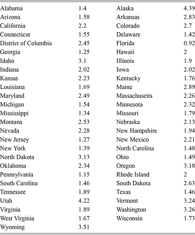
Table 4Long description
The table lists independent vote percentages in the 2020 election for all U.S. states and Districtic of Columbia. The top five are Alaska 4.39%, Utah 4.22%, Wyoming 3.51%, Vermont 3.24%, and Washington 3.26%. The bottom five are Florida 0.92%, Pennsylvania 1.15%, Georgia 1.25%, New Jersey 1.27%, and Mississippi 1.34%.
5.2 Model Fitting with MCMC Software
The MCMC software implementation JAGS is based on the language BUGS that was developed at Cambridge Biostatistics Unit and released in 1991 (Gilks, Thomas, & Spiegelhalter, Reference Gilks, Thomas and Spiegelhalter1994). It is a flexible and powerful platform developed by Martyn Plummer and is also distributed freely. The syntax is deliberately relatively R-like, but unlike R there are much fewer functions to work with because it is not intended to be an all-purpose statistical environment. JAGS can be run stand-alone but it is much easier to call it from R using the package rjags or in Python using the package PyJAGS.
There are five general steps to running the model and producing results:
1. Specify the distributional features of the model, and the quantities to be estimated in a text editor and import into R as a function.
2. Specify vectors for starting points and names of coefficients.
3. Run the model with the rjags function.
4. Assess convergence using the diagnostics in the R package superdiag.
5. Summarize empirically by variable as if the samples were data.
Most of the work is in the first step, but a nice feature of the software, especially the ones we focus on in this book, is that the model is specified very much as one would write it out on paper as shown in the following example. Interestingly, unlike other programming languages, statements are not processed serially, they constitute a full specification. Still, there is a structure to writing the code.
The default MCMC transition kernel in JAGS is the Gibbs sampler and therefore the first step in the software identifies the full conditional distributions for each variable in the model. This is done by the software not by the user. If the software cannot determine the full conditional distribution for a given parameter, then it automatically switches to the Metropolis–Hastings algorithm for that dimension only, making the result a hybrid sampler. These statements show the beauty of how this software is constructed: the user codes a statistical model and JAGS encodes the full conditional distributions for Gibbs sampling.
Since the JAGS syntax is the same for R and Python, it should be fairly easy to adapt the R JAGS code to Python and vice versa. PyJAGS provides a Python interface to JAGS, which uses the exact same JAGS syntax for model specification and Python code to specify data and run sampler. Therefore, instead of repeating the JAGS code for Python, we want to introduce PyMC for Python implementation of the Bayesian regression models, which is a popular probabilistic programming library for building Bayesian models in Python. Developed as an open-source project, PyMC offers a powerful and flexible platform for Bayesian statistical modeling. Also PyMC is built on top of Theano (now maintained as Aesara), a Python library that is for working with multi-dimensional arrays including computing gradients using automatic differentiation. This makes it particularly adept at handling more sophisticated models that involve large datasets and complex posterior distributions. The syntax of PyMC is intentionally Pythonic, making it accessible to users familiar with Python and conducive to integration into larger Python applications. Additionally, PyMC shares similarities with JAGS in its expressive model specification, making it relatively easy for R JAGS users to transition to PyMC. It should be noted that PyMC uses advanced MCMC algorithms such as the No-U-Turn Sampler (NUTS), a variant of Hamiltonian Monte Carlo (HMC), which is more efficient for high-dimensional parameter spaces.
5.2.1 Murder Sentencing in Georgia Data
In a seminal study, David C. Baldus, Charles Pulaski, and George Woodworth (e.g. the Baldus study) looked at the potential disparity in the imposition of the death sentence in Georgia based on the race of the murder victim and the race of the defendant (Baldus, Pulaski, & Woodworth, Reference Baldus, Pulaski and Woodworth1983). This is actually two studies, the second one examining about 762 cases with a murder conviction in Georgia from March 1973 to December 1979. The data contains 160 covariates, including legal background, crime description, and demographics. From the 1970 US Census 1,187,149 out of 4,589,575, or about 26%, of Georgia residents were Black. The death penalty was imposed during this time according to:
22% cases of Black defendant, White victim
8% cases of White defendant and White victim
1% of cases of Black defendant and Black victim
3% of cases of White defendant and Black victim.
The Baldus study was cited in the US Supreme Court case McClesky v. Kemp (1987), in which a Black defendant (McClesky) was sentenced to death for killing a White police officer in Georgia. The central argument was that the sentence violated the Equal Protection clause of the Fourteenth Amendment, since statistically he was more likely to get the death penalty since the victim was White. The Supreme Court rejected McClesky’s argument (5-4) on the grounds that statistical trends did not effectively prove the existence of discrimination among the jury who decided his particular case. Supreme Court McClesky was executed in 1991.
The outcome variable is sentence, which is dichotomous according to: 0= life sentence, and 1=death penalty given. Consider the general statement of the regression structure in (1.1) where we will now specify a link function that is appropriate for 0/1 outcomes. This is a preview of the regression models in Sections 6 and 7. Of the 160 possible variables we choose the 9 in Table 5 as explanatory variables for this example. We matched 287 out of 454 White cases to the existing 287 Black cases using Mahalanobis distance matching with Match in R (Sekhon, Reference Sekhon2008). Since the analysis is done in R (by calling JAGS using the rjags package) or in Python, we will store these data in a list that looks like the following code boxes. In these boxes we only show a representative fraction of the data for space purposes. Notice also that we include data size definitions first in the list as good programming practice. For R the equal sign is required here not the “<-” notation.
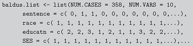
Code 1.011
 baldus.list <- list(NUM.CASES = 358, NUM.VARS = 10,
 sentence = c( 0, 1, 1, 0, 0, 0, 0, 0, 0, 0,...),
 race = c( 1, 1, 1, 1, 1, 1, 1, 1, 1, 1, 1,...),
 educatn = c( 2, 2, 3, 1, 2, 1, 1, 3, 2, 2,...),
 SES = c( 1, 1, 1, 1, 1, 1, 1, 1, 1, 1, 1,...),...
Code 1.012
 NUM_CASES = len(baldus_data)
 NUM_VARS = 10
 sentence = baldus_data[’sentence’].values
 race = baldus_data[’race’].values
 educatn = baldus_data[’educatn’].values
 SES = baldus_data[’SES’].values
 num_chld = baldus_data[ʼnum.chld’].values
 defense = baldus_data[’defense’].values
 vict_sex = baldus_data[’vict.sex’].values
 pr_incrc = baldus_data[’pr.incrc’].values
 aggrevat = baldus_data[’aggrevat’].values
 mitcir = baldus_data[’mitcir’].values
Generally, it is most convenient to write actual code in an ASCII text editor to create a file that the rjags or PyJAGS package functions can find. We will now break down the components of the logit regression model that models the dichotomous sentencing outcome. The outside structure of the model is simply a function definition in R with no terms passed-in:
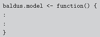
Code 1.013
 baldus.model <- function() {
 :
 :
 }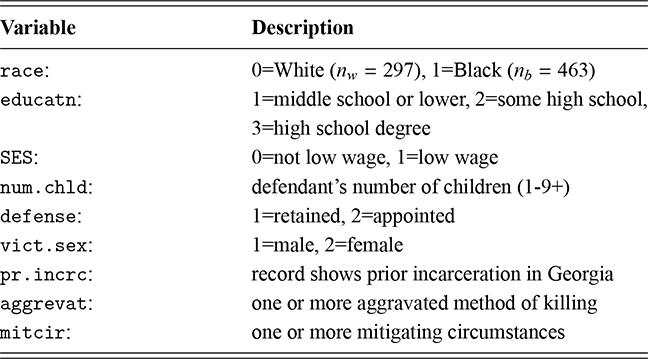
Table 5Long description
Each row defines a predictor and its coding: race (0 = White, 1 = Black), education level (1 - 3, 1 = middle school or lower, 3 = high school degree), socioeconomic status (0 = not low wage, 1 = low wage), number of children (1–9+), defense type (1 = retained, 2 = appointed), victim’s sex (1 = male, 2 = female), prior incarceration record, presence of aggravated methods, and presence of mitigating circumstances.
In PyMC, we use a model context to define model components, including the priors, likelihood, and the sampler. Model context is initiated using a with statement. This context manager encapsulates the entire model, ensuring that all the variables and definitions are scoped correctly within this block. The as model part will store this model context as an object called model in the environment, which can be called later.

Code 1.014
with pm.Model() as model: Now it is our responsibility to tell JAGS to loop through the data and perform a statistical procedure. This looks very much like a model written out by hand. First, we sum up the linear statistical component  by multiplying each variable per case by the corresponding coefficient to be estimated. The requirement in rjags is to put the link function on the left-hand side of the equation rather than specify the inverse link function on the right-hand side of the equation as most text books do: logit(p[i]). Here p[i] is the outcome variable for the
  th case. Notice that this is the exact structure identified in (1.1), where the link function is now the logit function:
 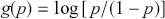 . Finally inside the cases loop we connect the outcome variable to the distributional assumption, which in this case is the Bernoulli PMF. This part of the code including the looping is shown in the following R code box. Just a reminder here that we will cover linear and nonlinear regression in much greater detail in the subsequent two sections.
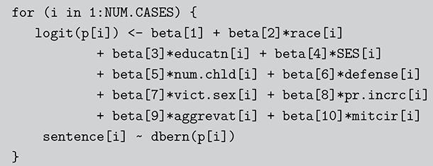
Code 1.015
 for (i in 1:NUM.CASES) {
 logit(p[i]) <- beta[1] + beta[2]*race[i]
 + beta[3]*educatn[i] + beta[4]*SES[i]
 + beta[5]*num.chld[i] + beta[6]*defense[i]
 + beta[7]*vict.sex[i] + beta[8]*pr.incrc[i]
 + beta[9]*aggrevat[i] + beta[10]*mitcir[i]
 sentence[i]   dbern(p[i])
 }
In PyMC, the model context will handle looping through the data and perform the statistical procedure. The model specification also closely mirrors the conceptual framework of the model. Unlike JAGS, where the link function is explicitly specified in the model structure, PyMC handles this through the sigmoid function on the right-hand side of the equation.

Code 1.016
 logit_p = (beta[0] + beta[1]*race +
 beta[2]*educatn + beta[3]*SES +
 beta[4]*num_chld + beta[5]*defense +
 beta[6]*vict_sex + beta[7]*pr_incrc +
 beta[8]*aggrevat + beta[9]*mitcir)
 p = pm.math.sigmoid(logit_p)
 sentence_obs = pm.Bernoulli(’sentence_obs’,
 p=p,
 observed=sentence)
Finally, since this is a Bayesian model, we need to specify the prior distributions. This is done in a very R-like syntax such as g.coef dgamma(alpha, beta), for each variable to be estimated. Here we could have done this 7 times for the seven beta coefficients, but it is more elegant to do it in a loop if they all get the same priors. This is why the betas are indexed. So now we add the final statement, which is outside the NUM.CASES loop in the NUM.VARS loop to finish the code.
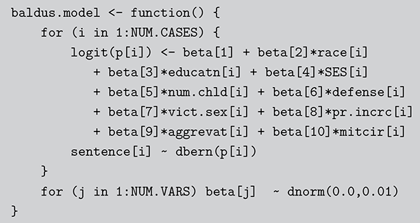
Code 1.017
 baldus.model <- function() {
 for (i in 1:NUM.CASES) {
 logit(p[i]) <- beta[1] + beta[2]*race[i]
 + beta[3]*educatn[i] + beta[4]*SES[i]
 + beta[5]*num.chld[i] + beta[6]*defense[i]
 + beta[7]*vict.sex[i] + beta[8]*pr.incrc[i]
 + beta[9]*aggrevat[i] + beta[10]*mitcir[i]
 sentence[i]   dbern(p[i])
 }
 for (j in 1:NUM.VARS) beta[j]   dnorm(0.0,0.01)
 }
Just as with JAGS, we start by defining the model, specifying priors, likelihoods, and, if necessary, transformations directly using the PyMC library. It also provides distribution functions to specify the prior distributions. In our case, we use the Normal() function to draw normal distributions with specified mu (mean) and sigma (standard deviation) for the priors of beta. The Normal() function also allows you to draw multiple values at a time by using the shape argument. One major difference between is that in PyMC the model specification and sampler need to be put in the same model context. PyMC code is also highly expressive just like rjags.
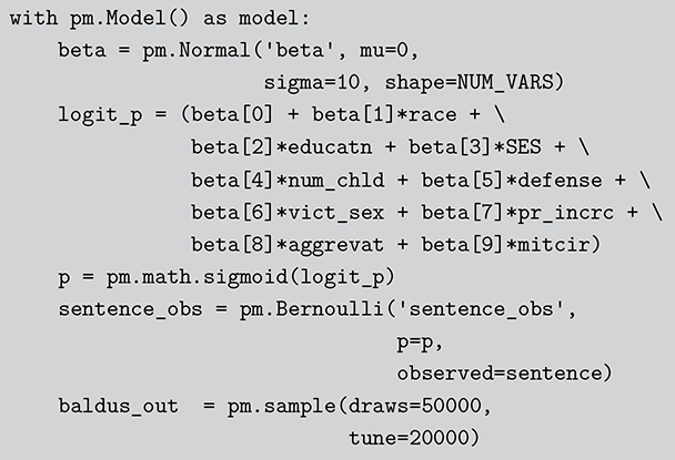
Code 1.018
 with pm.Model() as model:
 beta = pm.Normal(’beta’, mu=0,
 sigma=10, shape=NUM_VARS)
 logit_p = (beta[0] + beta[1]*race +
 beta[2]*educatn + beta[3]*SES +
 beta[4]*num_chld + beta[5]*defense +
 beta[6]*vict_sex + beta[7]*pr_incrc +
 beta[8]*aggrevat + beta[9]*mitcir)
 p = pm.math.sigmoid(logit_p)
 sentence_obs = pm.Bernoulli(’sentence_obs’,
 p=p,
 observed=sentence)
 baldus_out = pm.sample(draws=50000,
 tune=20000)
All JAGS models have essentially this structure above: loop through the data statements to provide the statistical model, separately specify the prior distributions on all of the unknown parameters in the model, and add any additional features as appropriate like longitudinal and hierarchical components. Now we need to identify a vector of starting points, and it is convenient to create a list of the coefficient names so as not to clutter up the model call. In this case since we indexed beta only a single character object is required. Calling rjags means specifying where the model, the data, the parameters, and the initial values are located. It is also required to specify the number of iterations. The full production of marginal posterior values involves two step shown below: create the model object, and then run this model object to draw samples. Note that in PyMC we don’t need a separate sampling procedure. The sampler is already defined in the model context and will run once we execute the code above.

Code 1.019
 baldus.inits <- list("beta" = rep(1,10))
 baldus.params <- c("beta")
 baldus.jags.obj <- jags.model(
 file="./BOOKS/Book.Bayes.IV/baldus.model.jags",
 data=baldus.list, inits=baldus.inits, n.chains = 1)
 baldus.out1 <- coda.samples(baldus.jags.obj,
 variable.names=baldus.params, n.iter=50000)
This produces the following output when we summarize the columns as data. These are deliberately portrayed as if from a standard logit regression although Bayesians usually prefer more information.
| Coef | StdErr | |
| (Intercept) | -3.44669686 | 1.11392418 |
| race | 0.87493310 | 0.28946874 |
| educatn | -0.01799630 | 0.19581014 |
| SES | -1.69381203 | 0.29300638 |
| num.chld | 0.01006399 | 0.08053441 |
| defense | 1.18060470 | 0.33752817 |
| vict.sex | 0.91479574 | 0.34767625 |
| pr.incrc | 0.22999805 | 0.32048919 |
| aggrevat | 1.00660730 | 0.42226770 |
| mitcir | -1.09579542 | 0.28368242 |
We see here five of the eight coefficients imply reliable effects with these point estimations: posterior means and standard errors. Consider the first two posterior coefficient distributions shown in Figure 5. For the race variable on the left (White=0, Black=1) we see that 0.0012 of the density (pictured in red) is below zero indicating that there is a 0.9982 probability that this effect is positive meaning that Black defendants are reliably more likely to get the death penalty than White defendants, given the model. For the education variable (middle school=1, some high school = 2, high school =3) the story is quite different: 0.5413 of the density is below zero meaning that we can make no reliable conclusion about the effect of this variable as there is a near equal probability of its effect being positive and negative. So posterior illustrations can be much more informative than standard regression tables.

Figure 5 Posterior Density for  and
and 
5.3 The Metropolis–Hastings Algorithm
Another MCMC algorithm that is commonly used, but we will feature less here, is the Metropolis–Hastings algorithm that was first created in 1953 (Metropolis et al., Reference Metropolis, Rosenbluth, Rosenbluth, Teller and Teller1953). This is a version of rejection sampling discussed in Section 3.3, where the candidate values are produced by a Markov chain instead of from a covering distribution as described previously. In this case the target distribution is the joint posterior distribution produced from the model specification,  . The Markov chain suggests a new destination
  from a distribution that is similar, but easy to draw from, called the candidate generating distribution,
  , which can but need not be conditional on the current position of the sampler,
  . Then an “acceptance ratio” is created by comparing the “desirability” of this new position relative to the current position
  according to the following formula:
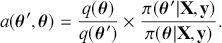 (5.5)
(5.5)
Then a uniform random variable is drawn between 0 and 1, denoted  . The new destination in the sample space is accepted if
  , otherwise the current position is chosen as the destination and a unit of time is consumed. So, unlike the Gibbs sampler, the Metropolis–Hastings algorithm does not have to move to a new location on each iteration. So one of three events can happen: (1) if there an ability to move to a higher density point the algorithm will always take it, (2) if there is a lower density point offered it will take it in proportion to the
  value drawn, meaning that lower
  values mean a lower probability of moving and vice versa, and (3) the proposal is rejected because
  . The structure of this algorithm actually leads to a lot more flexibility than the Gibbs sampler because the candidate generating process can be modified in many different ways to accommodate specific problems. Now that we have estimation tools required by more complex Bayesian models, we move on to Bayesian regression specifications.
6 Basic Bayesian Regression Models
Equipped with powerful computational techniques, we want to apply Bayesian methods in an analytical setting in the way typically undertaken by empirical social scientists. The regression model, first described in Equation (1.1) where the link function is just the identity function (no nonlinear effect), is one of the most widely used statistical tools and is one of the, if not the most, important tools statistics has given to mankind. It allows us to gauge the quality of the linear relationship between one or more explanatory variables ( ) and an outcome variable (
 ). This setup and its generalizations will be the common focus for the next few sections of this Element as we seek the marginal posterior distributions for
  under different modeling circumstances.
Bayesian linear regression models employ a fully probabilistic approach to estimate linear relationships between variables of interest. Unlike in classical regression where underlying parameters are assumed to be fixed by nature but unknown quantities that we estimate from the data, the Bayesian approach considers the regression parameters as random variables with specified prior distributions, which can be updated to posterior distributions with the likelihood function. This approach not only produces estimates of the parameters but also quantifies uncertainty in these estimates in a way that incorporates both prior beliefs and the likelihood of observing the data as first described in Section 2. In addition, Bayesian methods are also especially advantageous in their flexibility for model specifications and demonstrate robustness when applied to small datasets, making them particularly valuable in scenarios where conventional, non-Bayesian approaches struggle. The role of likelihood functions in general estimation and in Bayesian specifications was discussed in Section 3 of the companion work Gill and Bao (Reference Gill and Bao2024).
6.1 Linear Model and Likelihood Function
Begin with a simple linear model, which can be expressed conventionally as
 (6.1)
(6.1)
where  is a
is a  vector of outcome values,
  is a
is a  matrix of explanatory variables with a leading vector of ones for the constant,
  is a
is a  vector of coefficients to be estimated, and
  denotes an
  vector of error terms with mean zero and constant variance
  . Note this also means we assume homoscedasticity here: the error terms in the model have a constant variance across all levels of the explanatory variables. This is a reminder from Section 1 where the link function is the identity function in Equation (1.1).
The likelihood function is fundamental to estimating regression parameters in both conventional and Bayesian settings. It will help us find the most likely values of the unknown  and
and  given the observed and fixed data
  . For a sample of size
  , the likelihood function for the linear model is expressed conventionally as:
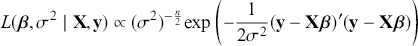 (6.2)
(6.2)
The term  gives the residuals, or the differences between the observed and estimated outcomes from the model using the current estimates of
  . The quantity
 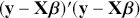 (or equivalently
 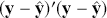 ) is known as the sum of squared errors. In conventional (non-Bayesian) settings, given the data is fixed, the focus is on finding the parameter values that maximize this likelihood function relative to the unknown parameter vector
  and
and  (as in the Maximum Likelihood Method), under normality. This approach alternatively leads to the exact same least squares estimates of the parameters as with ordinary least squares (OLS) method.
6.2 Prior and Posterior Distributions of Linear Models
Pivoting from the conventional setup to the Bayesian approach, instead of solely relying on the data to estimate parameters that are regarded as fixed, we now treat these parameters as random variables and incorporate prior knowledge and information about them. Setting prior distributions for regression parameters is obviously a necessary step here, as the priors, combined with the likelihood function, collectively shape the joint posterior distribution and the inferences we can draw from the model.
For one single coefficient parameter  , we could stipulate a normal distribution
  as a prior distribution, meaning that we believe the parameter
  is normally distributed around
  with variance
  before the data are observed. Frequently, if there is little prior information about the parameter
  , then researchers use a normal distribution with
  and a large
  . The prior distribution on the variance parameter
  reflects our assumptions about the variability or noise in the data, and is defined using distributions that are appropriate for variance parameters that are naturally bounded by
  . For example, we can define
  , which is an inverse gamma distribution with shape parameter
  and scale parameter
  . The inverse gamma PDF for parameters
  and
and  is given by the following formula:
 (6.3)
(6.3)
where the precision parameter  is then distributed
  .
.
The normal prior for coefficient parameter  and inverse gamma prior for variance parameter also conforms with the principles of conjugate priors in the Bayesian framework. Remember that conjugate priors are those that, when combined with a specific likelihood function, result in a posterior distribution that belongs to the same family as the prior (see more detailed discussion in Gill & Bao, Reference Gill and Bao2024). When the likelihood function of the observations is assumed to be normal, specifying a normal prior for
  results in a posterior that is also normal. For the variance
  , an inverse gamma prior and the squared error terms typically found in the likelihood of normal models also ensures the posterior variance is also an inverse gamma distribution.
It might be worth mentioning here that, if we specify improper uninformative priors such as a constant for  coefficients and a form of Jeffreys prior such as
  over the support of the entire possible ranges of the parameters (Tiao & Zellner, Reference Tiao and Zellner1964, p.220), the inferential results will be exactly the same as those obtained from a standard likelihood analysis of the linear model (Gill, Reference Gill2014, p.147). In this sense, the maximum likelihood solution can be viewed as equivalent to a Bayesian solution where the parameters are defined with improper uninformative priors over the entire support of the unknown parameters. This observation shows that the non-Bayesian approach to linear modeling is a special case of the Bayesian approach.
With the likelihood function and prior distributions, the vector joint posterior can be easily expressed as:
 (6.4)
(6.4)
where the posterior distribution  is proportional to the product of the prior distributions and the likelihood function. The posterior distribution now combines our initial beliefs (as informed by the priors) with the empirical evidence from the data (as articulated by the likelihood). It also offers a full probability distribution that reflects the uncertainties associated with the parameters instead of point estimates.
While closed-form solutions for some posterior distributions in Bayesian regression models are still possible under certain conditions (such as when using conjugate priors in the linear context), the practical limitations of these analytic solutions often become evident as the complexity of models increases. The good news is that, as we discussed in the previous section, MCMC empowers the Bayesian approach to handle even very complex settings where analytic solutions are not feasible.
6.3 Implementation in Software Packages
Starting in this section, we will be focusing on implementing Bayesian regression models using software libraries. For Bayesian linear models we will focus on an example of salaries for software developers based on the Stack Overflow Annual Developer Survey data in 2023. The data contains responses from Stack Overflow users on their demographics, coding skills, experience, work status, and compensation, as shown in Table 6 for the first six cases.

Table 6Long description
The table shows respondents’ age group, remote work status, education level, years of coding experience, and annual compensation. For example, the first respondent is a 25–34-year-old remote developer with a bachelor’s degree and nine years of coding experience earning $285k, while the second is a 45–54-year-old hybrid worker with 23 years of experience earning $250k.
We will employ a Bayesian linear regression model to assess the relationships between annual salary (in thousands of dollars) and predictors including age group, remote work arrangement, level of education, and years of professional coding experience. We write the model in “stacked notation” as:
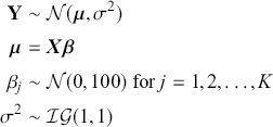 (6.5)
(6.5)
where the outcome variable  is assumed to be distributed with a mean
  and variance
  . Here,
  is defined as the product of an explanatory variable matrix
  and a vector of
  coefficients
  including the intercept. We stipulate a nearly flat prior with little prior influence on the
  term with an inverse gamma distribution.
Here we again employ JAGS with the R interface rjags to implement the model from in R. We also provide the procedure in Python in the following code box with the PyMC library. Note that, since the outcome variable is skewed, we will need to convert it to a logarithmic form when preparing the data.
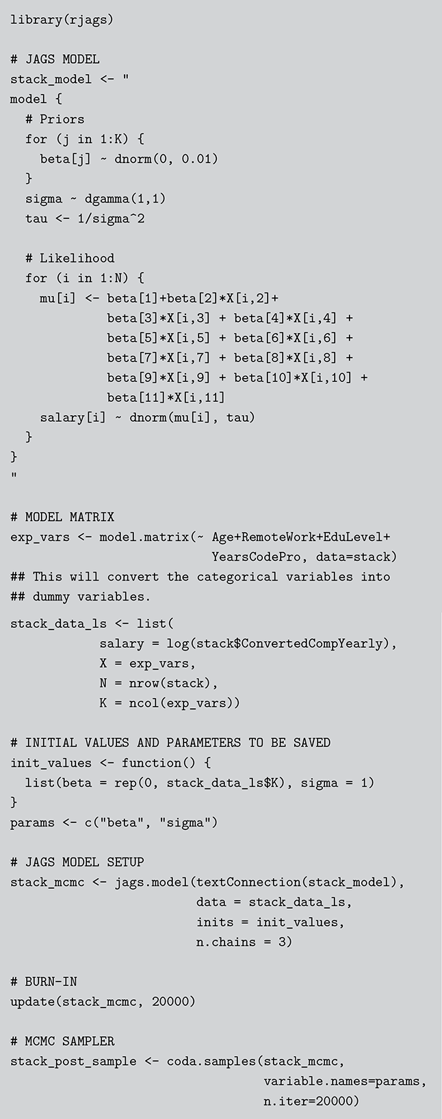
Code 1.020
 library(rjags)
 # JAGS MODEL
 stack_model <- "
 model {
 # Priors
 for (j in 1:K) {
 beta[j]   dnorm(0, 0.01)
 }
 sigma   dgamma(1,1)
 tau <- 1/sigma^2
 # Likelihood
 for (i in 1:N) {
 mu[i] <- beta[1]+beta[2]*X[i,2]+
 beta[3]*X[i,3] + beta[4]*X[i,4] +
 beta[5]*X[i,5] + beta[6]*X[i,6] +
 beta[7]*X[i,7] + beta[8]*X[i,8] +
 beta[9]*X[i,9] + beta[10]*X[i,10] +
 beta[11]*X[i,11]
 salary[i]   dnorm(mu[i], tau)
 }
 }
 "
 # MODEL MATRIX
 exp_vars <- model.matrix(  Age+RemoteWork+EduLevel+
 YearsCodePro, data=stack)
 ## This will convert the categorical variables into
 ## dummy variables.
 52stack_data_ls <- list(
 salary = log(stack$ConvertedCompYearly),
 X = exp_vars,
 N = nrow(stack),
 K = ncol(exp_vars))
 # INITIAL VALUES AND PARAMETERS TO BE SAVED
 init_values <- function() {
 list(beta = rep(0, stack_data_ls$K), sigma = 1)
 }
 params <- c("beta", "sigma")
 # JAGS MODEL SETUP
 stack_mcmc <- jags.model(textConnection(stack_model),
 data = stack_data_ls,
 inits = init_values,
 n.chains = 3)
 # BURN-IN
 update(stack_mcmc, 20000)
 # MCMC SAMPLER
 stack_post_sample <- coda.samples(stack_mcmc,
 variable.names=params,
 n.iter=20000)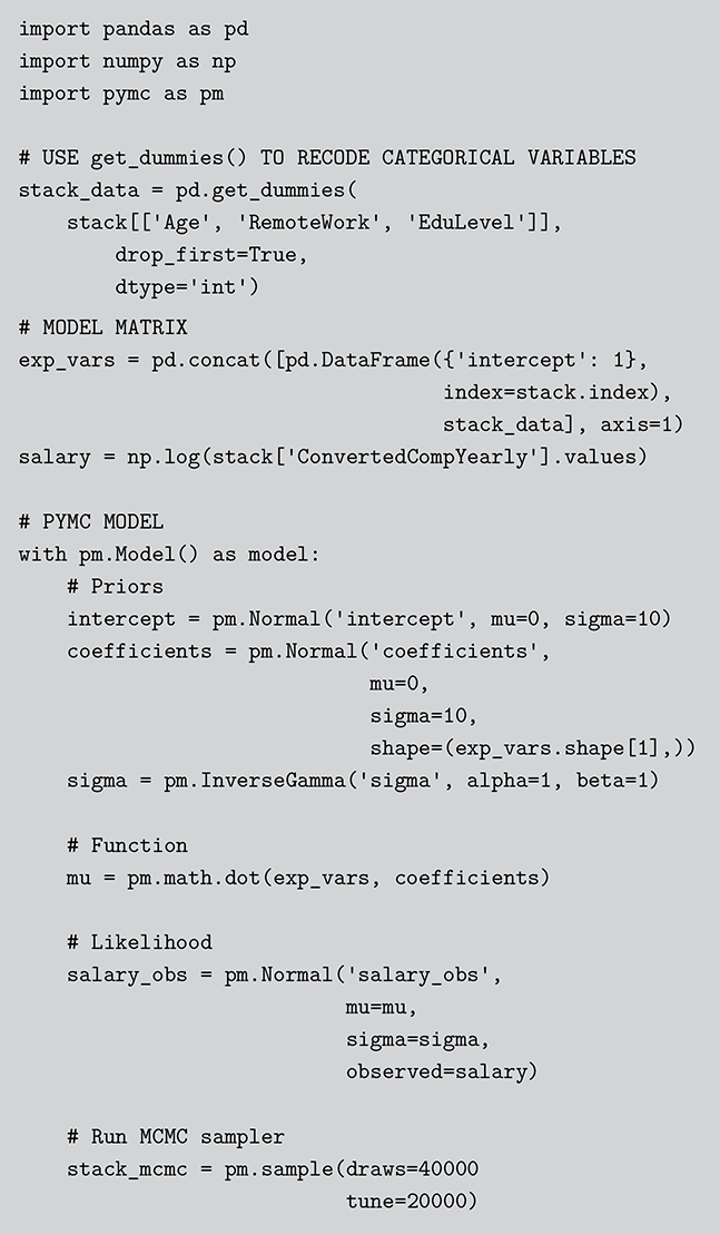
Code 1.021
 import pandas as pd
 import numpy as np
 import pymc as pm
 # USE get_dummies() TO RECODE CATEGORICAL VARIABLES
 stack_data = pd.get_dummies(
 stack[[’Age’, ’RemoteWork’, ’EduLevel’]],
 drop_first=True,
 dtype=’int’)
 53# MODEL MATRIX
 exp_vars = pd.concat([pd.DataFrame(’intercept’: 1,
 index=stack.index),
 stack_data], axis=1)
 salary = np.log(stack[’ConvertedCompYearly’].values)
 # PYMC MODEL
 with pm.Model() as model:
 # Priors
 intercept = pm.Normal(’intercept’, mu=0, sigma=10)
 coefficients = pm.Normal(’coefficients’,
 mu=0,
 sigma=10,
 shape=(exp_vars.shape[1],))
 sigma = pm.InverseGamma(’sigma’, alpha=1, beta=1)
 # Function
 mu = pm.math.dot(exp_vars, coefficients)
 # Likelihood
 salary_obs = pm.Normal(’salary_obs’,
 mu=mu,
 sigma=sigma,
 observed=salary)
 # Run MCMC sampler
 stack_mcmc = pm.sample(draws=40000
 tune=20000)
6.4 Understanding and Summarizing Posterior Distributions
The output generated by the MCMC sampler contains the entire set of posterior distributions of the parameters of interest, providing much richer information than the conventional single point estimates. These distributions capture the range of possible values for the parameters and inherent uncertainties given the data and model. Importantly, this feature also allows for a more natural depiction of the uncertainty. In contrast to conventional 95% confidence intervals, which are derived from point estimates and associated standard errors based on the assumption of repeated experiments, Bayesian highest probability density is a direct and intuitive representation of the simulated posterior results. In addition, the output posterior distribution allows us much greater flexibility when it comes to summarizing and reporting the results. The following code is the output posterior samples from JAGS for the preceding linear model. Using such information, we can directly compute various summary metrics from the posterior values. In the following output from rjags it notes that the thinning interval is equal to one. This information is no longer important and users should not manipulate this parameter in the call. Early in the 1990s when MCMC was new there was a perception that only recording every 10th value (or some other number) led to quicker production of reliable samples that could be treated as IID. It turns out that this is wrong since a sampler is either in its stationary distribution or not. In the stationary distribution there is obviously no need to subsample in this manner. A second concern at the time was that disk drives could get filled up with long MCMC runs. This is clearly no longer a concern.
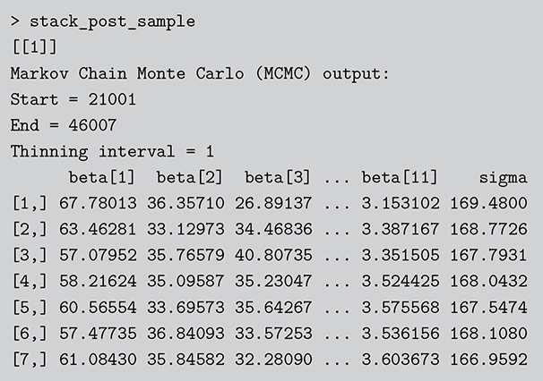
Code 1.022
 > stack_post_sample
 [[1]]
 Markov Chain Monte Carlo (MCMC) output:
 Start = 21001
 End = 46007
 Thinning interval = 1
 beta[1] beta[2] beta[3] ... beta[11] sigma
 [1,] 67.78013 36.35710 26.89137 ... 3.153102 169.4800
 [2,] 63.46281 33.12973 34.46836 ... 3.387167 168.7726
 [3,] 57.07952 35.76579 40.80735 ... 3.351505 167.7931
 [4,] 58.21624 35.09587 35.23047 ... 3.524425 168.0432
 [5,] 60.56554 33.69573 35.64267 ... 3.575568 167.5474
 [6,] 57.47735 36.84093 33.57253 ... 3.536156 168.1080
 [7,] 61.08430 35.84582 32.28090 ... 3.603673 166.9592
In the following, we use the default summary methods to summarize the MCMC posterior samples. We also manually calculate the mean, median, standard deviation, and 2.5% and 97.5% percentiles of the posterior distribution of the coefficient on years of code experience provided. Then, we can easily create a comprehensive summary of the posterior distribution for the regression parameters as in Table 7. While it is relatively common to summarize Bayesian models in this way. partly due to journal requirements, Bayesians often prefer graphical results. So we also provide the 95% HPDs in Figure 6.
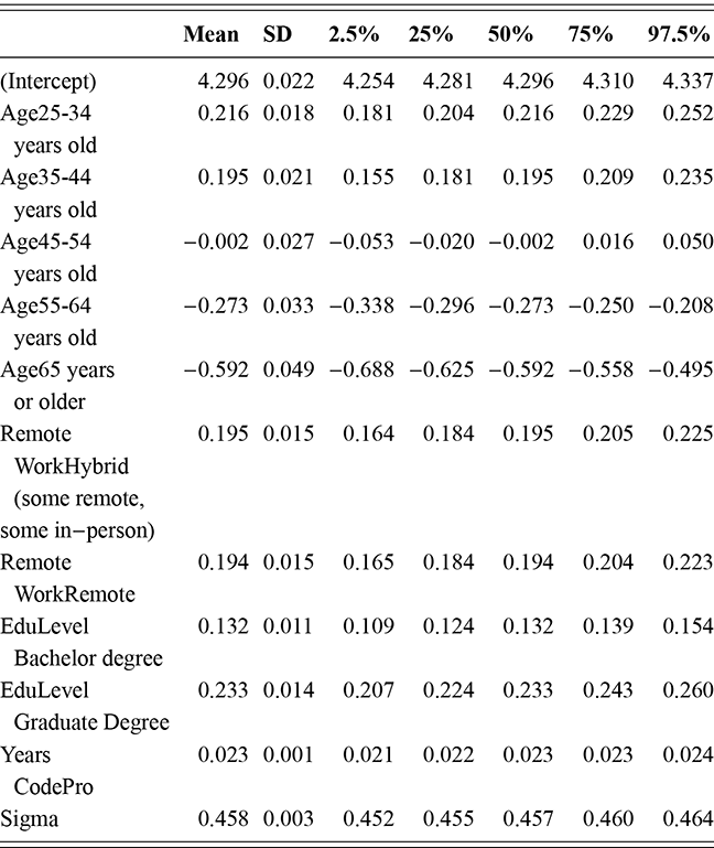
Table 7Long description
The table reports posterior means, standard deviations, and quantiles (2.5%, 25%, 50%, 75%, 97.5%) for model parameters, including age categories, remote work type, education level, years of coding experience, and sigma.

Figure 6 Highest Posterior Density Intervals, Stack Overflow Model
Code 1.023
 summary(stack_post_sample)
 # MANUALLY EXTRACT THE CHAIN AND CALCULATE STATISTICS
 mean(stack_post_sample[[1]][,11])
 56median(stack_post_sample[[1]][,11])
 sd(stack_post_sample[[1]][,11])
 quantile(stack_post_sample[[1]][,11], c(0.025, 0.975))
Code 1.024
 pm.summary(stack_mcmc)
 # EXTRACT THE FIRST CHAIN AND VARIABLE OF INTEREST
 beta11 = stack_mcmc.posterior.isel(
 chain=0,coefficients_dim_0=10).coefficients.values
 # MANUALLY CALCULATE STATISTICS
 mean_val = np.mean(beta11)
 median_val = np.median(beta11)
 std_val = np.std(beta11)
 quantiles = np.quantile(beta11, [0.025, 0.975])
This section presented the Bayesian linear regression model and estimation with MCMC. In the following section we present the same topics with Bayesian nonlinear regression models for noncontinuous outcome variables.
7 Nonlinear Bayesian Regression Models
Nonlinear regression models extend the linear models on the relationship between the collection of explanatory variables  and associated
  estimands, where the linear assumption for the relationship between
  and the expected values of
  or the normality of the error term
  is not appropriate. Nonlinear regression models include a diverse range of outcome types, including discrete choices, count data, survival times, and truncated variables, among others. Sometimes, nonlinear regression can also be framed within the context of generalized linear models, as GLMs extend the standard linear model by using link functions to transform the relationship between predictors and nonnormal outcome variables back into a linear form.
Bayesian methods provide a more holistic and robust framework for working with nonlinear models. Especially when combined with Markov Chain Monte Carlo (MCMC) techniques, Bayesian methods are able to effectively explore parameter spaces and quantify uncertainty. One practical advantage of the Bayesian approach in the context of nonlinear models is its capacity to provide solutions even in challenging scenarios where traditional methods may fail.
7.1 Nonlinear Regression Specifications
With a nonlinear relationship between the linear additive component  and the expected values of the outcome variable
  , the assumptions of the linear regression model do not hold. In this situation we use generalized linear models that specify a “link function” that accounts for nonlinear relationship. For instance, the outcome variables can be dichotomous, like the example in Section 7.2, then the mean of
  (could be interpreted as the probability) may be linearly related to
  , but the error term cannot be described by the normal distribution. Another example can be if the outcome variable is truncated (e.g. cases with income below a threshold are excluded from the sample), then both the mean and variance of
  are affected by the truncation, and they need to be modeled simultaneously, as misspecification of one parameter leads to inconsistent estimation of the other.
The idea of generalized linear models is to extend the normal linear model framework to accommodate outcomes with different levels of measurement. This approach generalizes various types of outcome variables with disparate mathematical forms to a common mathematical framework, which describes a linear relationship between the transformed linear additive component and the expected outcome vector. This framework allows for the modeling of various types of data by appropriately choosing the link function and the distribution family. Another extension is needed with truncated or censored outcomes. Truncated outcomes occur when the response variable is restricted to a certain range, such as when we only record the outcome above or below a threshold. Conversely censored outcomes happen when the response variable is only partially observed, for instance, if data points below or above certain thresholds are not fully recorded. Both types of outcomes require different specifications.
7.2 Logistic Regression
Logistic regression is used for modeling dichotomous or Bernoulli outcomes, typically represented as 0 (failure) and 1 (success) values. In logistic regression, the relationship between the explanatory variables  and the probability of the outcome
  is modeled using the logistic function, also known as the logit function. The logit function expresses this relationship in terms of odds rather than direct probabilities. The odds of an event are defined as the ratio of the probability that the event occurs to the probability that it does not:
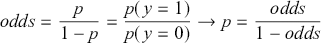 (7.1)
(7.1)
where odds is obviously on the support  . The log of the odds is modeled as follows:
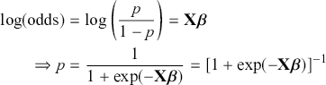 (7.2)
(7.2)
with the linear component  . Equation 7.2 is the logit link function
 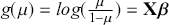 , which maps the linear predictor to the expected value of the outcome. Note there are also other different functions that can achieve this goal of modeling dichotomous outcomes such as probit and complementary log-log (clog-log). The probit link function is
 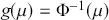 , where
  is the cumulative distribution function of the standard normal distribution. The clog-log link function is defined as
  , which is close to but not an exact approximation of the same mathematical form and also asymmetrical in
  (see Gill & Torres, Reference Gill and Torres2019, for more details). The differences between these different functions are mostly noticeable in the tails of these distributions, especially for cloglog, which is skewed.
Using the logit link function, we can derive the likelihood function for a dataset with  observations:
 (7.3)
(7.3)
where  is the probability that
  evaluating the model’s prediction for each instance where the outcome is 1;
 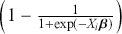 indicates the probability that
  .
.
The conventional approach to estimating the parameters in logistic regression is through the method of maximum likelihood estimation. To find the maximum likelihood estimates, it’s often more practical to work with the log-likelihood function 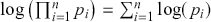 . However, the derivatives of the log-likelihood necessary for parameter estimation do not have straightforward analytical solutions, which further requires the use of numerical optimization techniques such as Gradient Descent or Newton–Raphson methods. These techniques need to iterate over potential solutions, incrementally adjusting the parameter estimates to maximize the likelihood, which is still sensitive to issues like starting values and local optima, particularly in complex models or those with issues like multicollinearity and separation.
The Bayesian approach with MCMC provides a more holistic approach here. Logistic regression can suffer from the problems of identification and separation, where the linear combination of the predictors perfectly predicts the dichotomous outcomes. With prior information, even a weak prior, the Bayesian approach can mitigate such common problems in logistic regression and also higher-order interactions, thus stabilizing the estimates (Gelman et al. Reference Gelman, Jakulin, Pittau and Su2008).
To illustrate Bayesian logistic regression, we consider a dataset from a study by Hopkins (Reference Hopkins2010) on how local conditions, especially the influx of immigrants, trigger local anti-immigration policies in the U.S. The data includes a series of demographic, economic, and political variables including household income, percent homeowner, unemployment, percent immigrants, population density, percent Black, and partisanship to explain whether the community has a local anti-immigrant ordinance as shown in Table 8.
| Variable | Description |
|---|---|
| EVENT3 | Indicates if there was a local ordinance identified by |
| Lexis-Nexis or FIRM | |
| LGMHINC00 | Logged median household income in the CDP, 2000 |
| LGMHINCD90S | Change in the logged median household income, |
| 1990–2000 | |
| PCTOWND90S.x | Percent of homes that were owner-occupied, 2000 |
| PCTOWN00.x | Percent of homes that were owner-occupied, 2000 |
| unemployrate91.x | 1991 unemployment rate |
| unemployrateD90S | Change in unemployment rate, 1991–2000 |
| PCIMMD90S.x | Place’s share of foreign born, 1990 |
| PCIMM00.x | Place’s share of foreign born, 2000 |
| DENSIT | Population density, 2000 |
| PCNHBL00.x | Place percent non-Hispanic Black, 2000 |
| PCNHBLD90S.x | Place percent non-Hispanic Black, change from |
| 1990–2000 | |
| dempct88.x | Percent of country backing Democratic presidential |
| candidate, 1988 |
The model is specified as follows in stacked notation as:
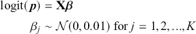 (7.4)
(7.4)
where  represents the logit link function mapping the probability
  (bounded between 0 and 1) to the linear component
  . We stimulate normal distributions with mean zero for the
  coefficients and a gamma distribution for the precision parameter of the normal distribution.
The neat thing is we can write this model exactly like this in R and Python. The code in the following box implements the model with rjags and pymc. In JAGS, the logit function directly transforms the linear predictor into probabilities. The logit(p[i]) expression applies the logit transformation, where 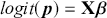 . Then, y[i]
  dbern(p[i]) models the binary outcome as a Bernoulli trial with success probability
  . In PyMC, the pm.math.sigmoid function serves as the logit transformation, converting the linear combination of predictors
  into probabilities p in the
  range. The binary outcome is then modeled using pm.Bernoulli, which takes the probability
  for each observation. The results of the model are also shown in Table 9.
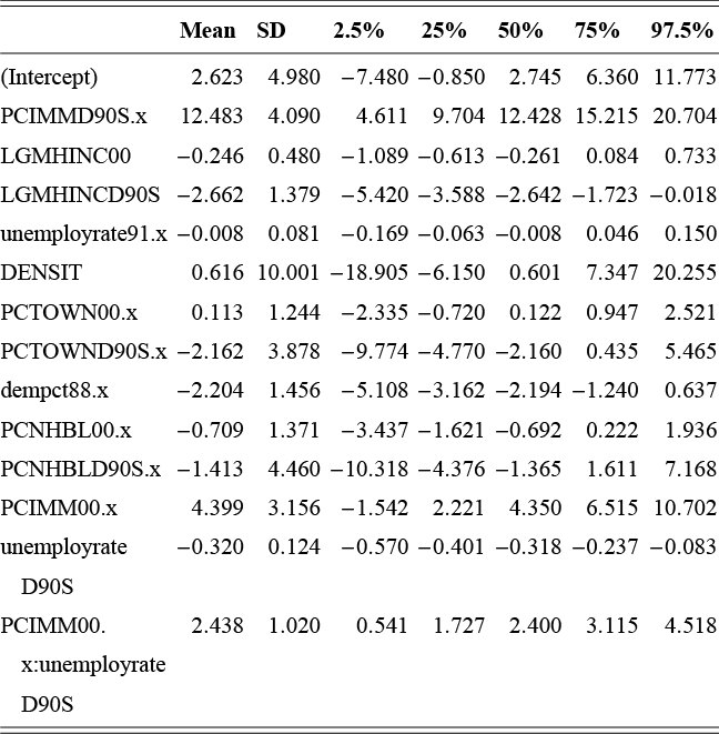
Table 9Long description
The table reports posterior means, standard deviations, and quantiles (2.5%, 25%, 50%, 75%, 97.5%) for model parameters, including demographic, economic, and policy variables, as well as interaction terms.

Code 1.025
 library(rjags)
 immigration <- read.csv("data/immigration.csv")
 immigration_model <- "
 model {
 # Priors
 for (j in 1:K) {
 beta[j]   dnorm(0, 0.01)
 }
 62# LIKELIHOOD FUNCTION
 for (i in 1:N) {
 logit(p[i]) <- beta[1] + beta[2]*X[i,2]+
 beta[3]*X[i,3] + beta[4]*X[i,4]+
 beta[5]*X[i,5] + beta[6]*X[i,6]+
 beta[7]*X[i,7] + beta[8]*X[i,8]+
 beta[9]*X[i,9] + beta[10]*X[i,10]+
 beta[11]*X[i,11] + beta[12]*X[i,12]+
 beta[13]*X[i,13] + beta[14]*X[i,14]
 # BINARY OUTCOME
 y[i]   dbern(p[i])
 }
 }
 "
 exp_vars <- model.matrix(  PCIMMD90S.x+LGMHINC00+
 LGMHINCD90S+unemployrate91.x+DENSIT+
 PCTOWN00.x+PCTOWND90S.x+dempct88.x+
 PCNHBL00.x+PCNHBLD90S.x+
 PCIMM00.x*unemployrateD90S,
 data = immigration)
 immigration_data <- list(y = immigration$EVENT3,
 X = exp_vars,
 N = nrow(immigration),
 K = ncol(exp_vars))
 params <- c("beta")
 init_values <- function() {
 list(beta = rep(0, immigration_data$K))
 }
 immigration_model <- jags.model(
 textConnection(immigration_model),
 data = immigration_data,
 inits = init_values,
 n.chains = 3)
 update(immigration_model, 25000)
 immigration_mcmc <- coda.samples(immigration_model,
 63variable.names = "beta",
 n.iter = 25000)
 summary(immigration_mcmc)
Code 1.026
 import numpy as np
 import pandas as pd
 import pymc as pm
 immigration = pd.read_csv("data/immigration.csv")
 exp_vars = pd.concat([pd.DataFrame(
 ’intercept’: 1,
 index=immigration.index),
 immigration[[
 ’PCIMMD90S.x’,’LGMHINC00’,
 ’LGMHINCD90S’,’unemployrate91.x’,
 ’DENSIT’,’PCTOWN00.x’,
 ’PCTOWND90S.x’,’dempct88.x’,
 ’PCNHBL00.x’,’PCNHBLD90S.x’,
 ’PCIMM00.x’,
 ’unemployrateD90S’]]],
 axis=1)
 exp_vars[’PCIMM00.x:unemployrateD90S’] =
 exp_vars[’PCIMM00.x’] * exp_vars[’unemployrateD90S’]
 X = exp_vars.values
 y = immigration[’EVENT3’].values
 N, K = X.shape
 with pm.Model() as immigration_model:
 # Priors
 beta = pm.Normal(’beta’, mu=0, sigma=10, shape=K)
 # Likelihood
 p = pm.math.sigmoid(pm.math.dot(X, beta))
 y_obs = pm.Bernoulli(’y_obs’, p=p, observed=y)
 64# Sampling
 immigration_mcmc = pm.sample(draws=50000,
 tune=25000)
 pm.summary(immigration_mcmc)
7.3 Poisson Model
Count data are often modeled using a Poisson regression (also called log-linear), which is another type of generalized linear model. In the Poisson model, the outcome variable represents the number of occurrences of an event within a fixed period of time or space. These counts  are assumed to be Poisson-distributed with mean
  (and therefore variance is
  as well):
 (7.5)
(7.5)
where 
 is called the intensity parameter, representing the expected number of occurrences in the fixed interval.
To model the relationship between the count data and predictor variables, we use Poisson regression. In Poisson regression, the logarithm of  is modeled as a linear function of the predictors
  . This ensures that the rate parameter
  remains positive regardless of the values of
  and the coefficients
  . The model is expressed as follows:
 (7.6)
(7.6)
where  of the count variable
  connects to the linear predictors through a log link function. Given the model specifications, the likelihood function for a set of observations
  is:
is:
 (7.7)
(7.7)
where  is the predicted mean count for the
  -th observation. For Bayesian Poisson regression, we again need to define the prior distribution for the
  coefficients, often chosen as normal distributions. The posterior distribution is then again formed by combining the likelihood of the observed data with the priors.
| Variable | Description |
|---|---|
| num_tweets | Count of tweets about homeschooling |
| age | Age group of the respondent |
| female | Indicator for female (female = 1) |
| race | Race of the respondent |
| inc | Income level |
| college | Indicator for whether the respondent has a college degree |
| party_id | Political affiliation |
| employ | Employment status (employed = 1) |
| kids | Having children at home |
| vaccine | Vaccination status (vaccinated = 1) |
To illustrate Bayesian Poisson regression, we examine an example of tweets about homeschooling during the COVID-19 pandemic. This dataset contains survey responses from 316 participants, each linked to their Twitter activity data, including the number of tweets specifically about homeschooling. The variables in this dataset are listed in Table 10.
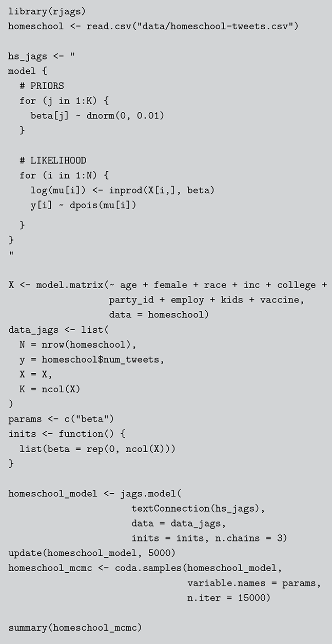
Code 1.027
 library(rjags)
 homeschool <- read.csv("data/homeschool-tweets.csv")
 hs_jags <- "
 model {
 # PRIORS
 for (j in 1:K) {
 beta[j]   dnorm(0, 0.01)
 }
 # LIKELIHOOD
 for (i in 1:N) {
 log(mu[i]) <- inprod(X[i,], beta)
 y[i]   dpois(mu[i])
 }
 }
 "
 X <- model.matrix(  age + female + race + inc + college +
 party_id + employ + kids + vaccine,
 data = homeschool)
 data_jags <- list(
 N = nrow(homeschool),
 y = homeschool$num_tweets,
 X = X,
 K = ncol(X)
 )
 params <- c("beta")
 inits <- function() {
 list(beta = rep(0, ncol(X)))
 }
 homeschool_model <- jags.model(
 textConnection(hs_jags),
 data = data_jags,
 inits = inits, n.chains = 3)
 update(homeschool_model, 5000)
 homeschool_mcmc <- coda.samples(homeschool_model,
 variable.names = params,
 n.iter = 15000)
 summary(homeschool_mcmc)
The implementation of the Bayesian Poisson Model in R and Python is similar to other GLMs. The key is to define the link function. For JAGS, we use the dpois() distribution function; for PyMC, we use the Poisson() function. The code also shows one key difference between JAGS and PyMC here. In Python, we cannot add functions to the left hand of the equation like in R (logit()), so we need to specify the inverse link function pm.math.exp() on the right-hand side. The output of the Poissson model estimating the effects on the number of homeschooling-related tweets is shown in Table 11.

Code 1.028
 import pandas as pd
 import numpy as np
 import pymc as pm
 homeschool = pd.read_csv("data/homeschool-tweets.csv")
 homeschool = pd.get_dummies(homeschool, columns=[’age’,
 ’race’, ’inc’, ’party_id’],
 drop_first=True, dtype=’int’)
 X = homeschool[[’female’, ’college’, ’employ’, ’kids’,
 ’vaccine’] +
 [col for col in homeschool.columns if
 col.startswith((’age_’, ’race_’, ’inc_’,
 ’party_id_’))]]
 X.insert(0, ’intercept’, 1) # Add intercept column
 N = X.shape[0]
 K = X.shape[1]
 y = homeschool[ʼnum_tweets’].values
 X = X.values
 with pm.Model() as model:
 # PRIORS FOR REGRESSION PARAMETERS
 beta = pm.Normal(’beta’, mu=0, sigma=10, shape=K)
 # LINEAR PREDICTOR
 mu = pm.math.exp(pm.math.dot(X, beta))
 # LIKELIHOOD
 y_obs = pm.Poisson(’y_obs’, mu=mu, observed=y)
 # SAMPLING
 trace = pm.sample(draws=15000, tune=5000,
 target_accept=0.95)
 summary = pm.summary(trace, var_names=[’beta’])
 print(summary)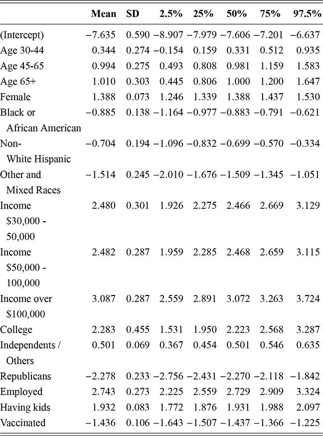
Table 11Long description
The table reports posterior means, standard deviations, and quantiles (2.5%, 25%, 50%, 75%, 97.5%) for parameters representing demographic, socioeconomic, and political variables, including age, gender, race, income categories, education, employment, and vaccination status.
7.4 Truncated Outcome Models
Even when data follow the normal linear pattern, they do not always appear perfectly as expected. One such case is when the data are truncated, meaning the sample is only observed within certain limits of the outcome variables. For example, consider a study on the impact of education on income, but the data only include individuals with incomes above a certain threshold, thus truncating the lower end of the income distribution. These types of data are commonly encountered in scenarios where observations with outcomes below or above specific thresholds are not observed or are excluded due to measurement limitations or study design. In such cases standard linear models that do not account for truncation can lead to biased estimates and illogical predictions.
Consider a case where the outcome variable  is truncated from below at threshold
  and from above at threshold
  (
( ). The probability density function of the truncated normal distribution is derived from the standard normal distribution but adjusted for the truncation:
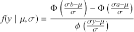 (7.8)
(7.8)
where  is the probability density function and
  is the cumulative distribution function of the standard normal distribution. Given a sample of
  observations with the outcome
  from a truncated normal distribution and the linear component modeled as
  . The likelihood function is given by:
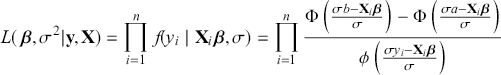 (7.9)
(7.9)
The key issue here is to specify the likelihood function to account for the fact that the data are observed within certain limits.
To demonstrate the truncated outcome model, we use an example of home loan approvals from a real estate financing company. In this example, the minimum loan amount set by the company is $25,000. As a result, any cases where applicants would qualify for a loan amount below $25,000 are not recorded in the data. Consequently, the observed data only includes loan amounts of $25,000 or more, creating a left-truncated dataset. The data contains the information shown in Table 12
We specify a truncated normal regression model to predict the loan amount ( ) received by applicants based on various factors (
 ). The outcome variable,
  , is truncated at 25 (thousands of dollars):
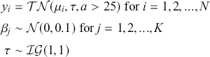 (7.10)
| Variable | Description |
|---|---|
| Gender | Male / Female |
| Married | Applicant married (Y/N) |
| Dependents | Number of dependents |
| Education | Applicant Education (Graduate / Under Graduate) |
| Self_Employed | Self-employed (Y/N) |
| ApplicantIncome | Applicant’s income |
| CoapplicantIncome | Co-applicant income |
| Credit_History | Credit history |
| Property_Area | Property area (Rural/ Semiurban / Urban) |
| LoanAmount | Loan amount in thousands |

Table 13Long description
The table reports posterior means, standard deviations, and quantiles (2.5%, 25%, 50%, 75%, 97.5%) for parameters including gender, marital status, number of dependents, education, employment type, applicant and coapplicant income, credit history, location type, and the variance parameter (sigma squared).
JAGS uses the T(,) construct to indicate truncation. This construct modifies the likelihood to indicate that the observed data is truncated. For example, if the outcome is normally distributed but with the truncation between  , JAGS can specify this as dnorm(mu, tau) T(a,b). In PyMC, TruncatedNormal() function is to define a normal distribution with specified mean (mu), precision (tau) or variance (sigma), and bounds (lower and upper). The results of the truncated normal model are shown in Table 13.
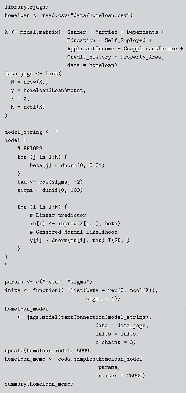
Code 1.029
 library(rjags)
 homeloan <- read.csv("data/homeloan.csv")
 X <- model.matrix(  Gender + Married + Dependents +
 Education + Self_Employed +
 ApplicantIncome + CoapplicantIncome +
 Credit_History + Property_Area,
 data = homeloan)
 data_jags <- list(
 N = nrow(X),
 y = homeloan$LoanAmount,
 X = X,
 K = ncol(X)
 )
 model_string <- "
 model {
 # PRIORS
 for (j in 1:K) {
 beta[j]   dnorm(0, 0.01)
 }
 tau <- pow(sigma, -2)
 sigma   dunif(0, 100)
 for (i in 1:N) {
 # Linear predictor
 mu[i] <- inprod(X[i, ], beta)
 # Censored Normal likelihood
 y[i]   dnorm(mu[i], tau) T(25, )
 }
 }
 "
 params <- c("beta", "sigma")
 inits <- function() {list(beta = rep(0, ncol(X)),
 sigma = 1)}
 72homeloan_model
 <- jags.model(textConnection(model_string),
 data = data_jags,
 inits = inits,
 n.chains = 3)
 update(homeloan_model, 5000)
 homeloan_mcmc <- coda.samples(homeloan_model,
 params,
 n.iter = 25000)
 summary(homeloan_mcmc)
Code 1.030
 import pandas as pd
 import numpy as np
 import pymc as pm
 homeloan = pd.read_csv("data/homeloan.csv")
 homeloan[’Gender’] = homeloan[’Gender’].map({’Male’: 1,
 ’Female’: 0})
 homeloan[’Married’] = homeloan[’Married’].map({’No’: 0,
 ’Yes’: 1})
 homeloan[’Education’]
 = homeloan[’Education’].map({’Not Graduate’: 0,
 ’Graduate’: 1})
 homeloan[’Self_Employed’]
 = homeloan[’Self_Employed’].map({’No’: 0,
 ’Yes’: 1})
 homeloan = pd.get_dummies(homeloan,
 columns=[’Dependents’, ’Property_Area’],
 drop_first=True, dtype=’int’)
 X = pd.concat([pd.DataFrame({’intercept’: 1},
 index=homeloan.index),
 homeloan[[’Gender’, ’Married’,
 ’Dependents_1’, ’Dependents_2’,
 ’Dependents_3+’, ’Education’,
 ’Self_Employed’,
 ’ApplicantIncome’,
 ’CoapplicantIncome’,
 ’Credit_History’,
 ’Property_Area_Semiurban’,
 ’Property_Area_Urban’]]], axis=1)
 N = X.shape[0]
 K = X.shape[1]
 y = homeloan[’LoanAmount’].values
 with pm.Model() as model:
 # PRIORS FOR REGRESSION COEFFICIENTS
 beta = pm.Normal(’beta’, mu=0, sigma=10, shape=K)
 sigma = pm.Uniform(’sigma’, lower=0.001, upper=100)
 tau = pm.Deterministic(’tau’, 1 / sigma**2)
 # LINEAR PREDICTOR
 mu = pm.math.dot(X, beta)
 # TRUNCATED NORMAL LIKELIHOOD
 y_obs = pm.TruncatedNormal(’y_obs’, mu=mu, tau=tau,
 lower=25, observed=y)
 # SAMPLING
 homeloan_mcmc = pm.sample(draws=25000, tune=5000,
 target_accept=0.95, cores=4)
 print(pm.summary(homeloan_mcmc,
 var_names=[’beta’, ’sigma’]))
Now that we have covered Bayesian linear regression model and the most common nonlinear forms, we return to the discussion of MCMC tools specifically on the important consideration of Markov chain convergence as well as how MCMC can be used to assess and compare fitted models.
8 Model Evaluation and Mechanical Issues with MCMC Estimation
In this section, we focus on several mechanical and practical issues essential to Bayesian analysis and MCMC. These include evaluating model fit and comparing models – tasks that, while not unique to Bayesian analysis, are approached in ways distinct to the Bayesian framework. Since Bayesian estimation depends on simulations that closely approximate the true posterior distribution, convergence diagnostics are crucial to ensure the reliability of the results. Additionally, the simulation-based nature of MCMC offers flexible ways to engage with models, leveraging the rich information from simulations to make predictions or compute quantities of interest, which can seamlessly incorporates uncertainty inherent in the simulation process.
8.1 Model Fit and Model Comparison
8.1.1 Bayes Factor
As introduced in Section 2, the Bayes factor can evaluate the relative evidence for competing models by comparing their marginal likelihoods, essentially allowing us to assess how well alternative statistical models explain the data. This is particularly useful in regression modeling, where we sometimes need to compare models with different predictors or complexity levels. For instance, we might ask whether including a specific variable or interaction term improves the model prediction, or if it unnecessarily complicates the model.
We can use the Bayes factor to compare two alternatives, not necessarily nested, linear model specifications. Using (6.2) with indexing, the likelihood function for model  is:
is:
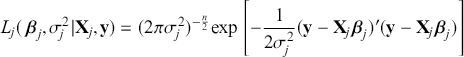 (8.1)
(8.1)
where  providing models
  and
and  . Here
  is not indexed since both models intend to explain the structure of the same outcome. To simplify the notation, make the definitions
 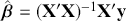 , and
, and  . Specify conjugate priors for each of these models with
  columns of
  according to:
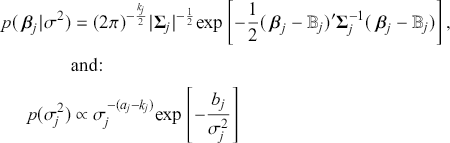
where  is the prior mean vector for
  . Add a multiplier
  on the variance term in the normal prior for
  :
:  . Here
  scales our subjective assessment of the reliability of
  , although it is set to 1 in typical practice. Make the common choice of prior mean for
  to be
to be  in both models. Now the marginal likelihood (the denominator from the right-hand side of Bayes’ law) for models
  and
and  from this setup is
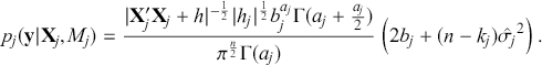 (8.2)
(8.2)
In practice, we often work with the log marginal likelihoods rather than original marginal likelihoods. For the model  , the log marginal likelihood can be expressed as follows:
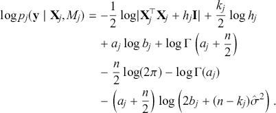 (8.3)
(8.3)
The difference in log marginal likelihoods between two models can then be exponentiated to compute the Bayes factor:
 (8.4)
(8.4)
Here we have a longish but not complicated structure that is easy to program in R or Python. Using the example of linear model with Stack Overflow data, we may want to see if including the variable RemoteWork improved the model for yearly compensation. We compare the full model (with all predictors) to the reduced model (excluding RemoteWork). The following R and Python code computes the log marginal likelihoods and Bayes factor:

Code 1.031
 library(MASS)
 # LOG MARGINAL LIKELIHOOD FUNCTION
 log_marginal_likelihood <- function(X, y, h, a, b) {
 n <- nrow(X)
 k <- ncol(X)
 76beta_hat <- solve(t(X) %*% X) %*% t(X) %*% y
 sigma_hat2 <- sum((y - X %*% beta_hat)^2)/(n-k)
 XtX_h <- t(X) %*% X + diag(h, k)
 log_marginal_likelihood <-
 -0.5 * log(det(XtX_h)) +
 0.5 * k * log(h) +
 a * log(b) + lgamma(a + n/2) -
 (n/2) * log(2 * pi) - lgamma(a) -
 (a + n/2) * log(2 * b + (n-k) * sigma_hat2)
 return(log_marginal_likelihood)
 }
 log_ml_full <- log_marginal_likelihood(
 exp_vars,
 log(stack$ConvertedCompYearly),
 h=1, a=1, b=1)
 log_ml_reduced <- log_marginal_likelihood(
 exp_vars_reduced,
 log(stack$ConvertedCompYearly),
 h=1, a=1, b=1)
 (bayes_factor <- exp(log_ml_full-log_ml_reduced))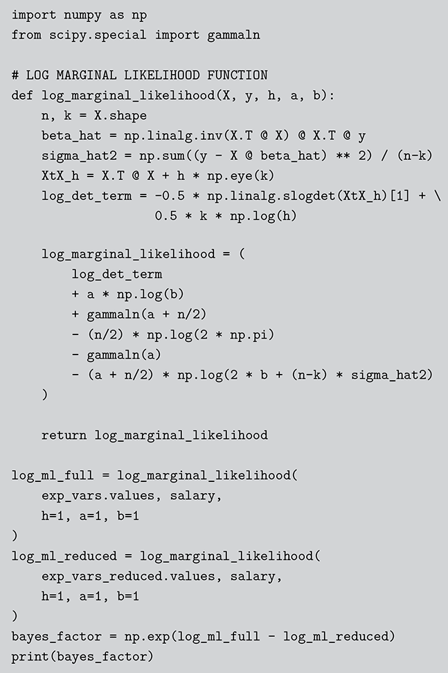
Code 1.032
 import numpy as np
 from scipy.special import gammaln
 # LOG MARGINAL LIKELIHOOD FUNCTION
 def log_marginal_likelihood(X, y, h, a, b):
 n, k = X.shape
 beta_hat = np.linalg.inv(X.T @ X) @ X.T @ y
 sigma_hat2 = np.sum((y - X @ beta_hat) ** 2) / (n-k)
 XtX_h = X.T @ X + h * np.eye(k)
 log_det_term = -0.5 * np.linalg.slogdet(XtX_h)[1] +
 0.5 * k * np.log(h)
 77log_marginal_likelihood = (
 log_det_term
 + a * np.log(b)
 + gammaln(a + n/2)
 - (n/2) * np.log(2 * np.pi)
 - gammaln(a)
 - (a + n/2) * np.log(2 * b + (n-k) * sigma_hat2)
 )
 return log_marginal_likelihood
 log_ml_full = log_marginal_likelihood(
 exp_vars.values, salary,
 h=1, a=1, b=1
 )
 log_ml_reduced = log_marginal_likelihood(
 exp_vars_reduced.values, salary,
 h=1, a=1, b=1
 )
 bayes_factor = np.exp(log_ml_full - log_ml_reduced)
 print(bayes_factor)
In a more Bayesian way, we can also obtain the marginal likelihoods by drawing samples from the posterior distribution. This is especially handy in the situations where the integral becomes computationally intractable. The marginal likelihood for a model  integrates the likelihood of the data
  over the entire parameter space, weighted by the prior
  :
:
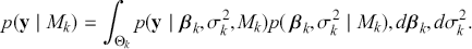 (8.5)
(8.5)
Using the MCMC posterior samples, the marginal likelihood can be approximated using Monte Carlo methods as follows:
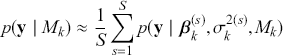 (8.6)
(8.6)
where  is the number of posterior samples. This involves evaluating the likelihood
 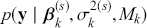 for each posterior draw. Again, we work with the log marginal likelihood:
 (8.7)
(8.7)
Using the log-sum-exp trick, it can further be computed as follows:
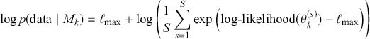 (8.8)
(8.8)
In the following R and JAGS code, we can obtain the MCMC posterior samples for the reduced model. The full model remains similar to earlier examples, with the key addition of extracting log-likelihoods from the JAGS output. These log-likelihoods allow us to approximate the marginal likelihoods for model comparison.

Code 1.033
 ## REDUCED MODEL
 stack_reduced_model <- "
 model {
 # Priors
 for (j in 1:K) {
 beta[j]   dnorm(0, 0.01)
 }
 sigma   dgamma(1,1)
 tau <- 1/sigma^2
 # LIKELIHOOD
 for (i in 1:N) {
 salary[i]   dnorm(mu[i], tau)
 mu[i] <- beta[1]+beta[2]*X[i,2]+
 beta[3]*X[i,3]+beta[4]*X[i,4]+beta[5]*X[i,5]+
 beta[6]*X[i,6]+beta[7]*X[i,7]+beta[8]*X[i,8]+
 beta[9]*X[i,9]
 loglik[i] <- logdensity.norm(salary[i], mu[i], tau)
 }
 }
 "
 79exp_vars_reduced <- model.matrix(
   Age+EduLevel+YearsCodePro,
 data=stack)
 stack_reduced_ls <- list(
 salary = log(stack$ConvertedCompYearly),
 X = exp_vars_reduced,
 N = nrow(stack),
 K = ncol(exp_vars)-2)
 init_values <- function() {
 list(beta = rep(0, stack_reduced_ls$K), sigma = 1)
 }
 params <- c("beta", "sigma")
 stack_mcmc_reduced <- jags.model(
 textConnection(
 stack_reduced_model),
 data = stack_reduced_ls,
 inits = init_values,
 n.chains = 3)
 update(stack_mcmc_reduced, 20000)
 stack_reduced_sample <- coda.samples(
 stack_mcmc_reduced,
 variable.names=c("loglik"),
 n.iter=20000)
 # EXTRACT LIKELIHOODS
 loglik_full <- do.call(rbind,
 lapply(stack_full_sample,
 as.matrix))
 loglik_sum_full <- rowSums(loglik_full)
 loglik_reduced <- do.call(rbind,
 lapply(stack_reduced_sample,
 as.matrix))
 loglik_sum_reduced <- rowSums(loglik_reduced)
 # LOG-MEAN-EXP FUNCTION
 logmeanexp <- function(x) {
 80max_x <- max(x)
 return(max_x + log(mean(exp(x - max_x))))
 }
 (log_marginal_full <- logmeanexp(loglik_sum_full))
 (log_marginal_reduced <- logmeanexp(loglik_sum_reduced))
 (bayes_factor <- exp(log_marginal_full -
 log_marginal_reduced))
A slight difference between the R and Python implementations lies in how log-likelihoods are handled. In R and JAGS the logdensity.norm function computes log-likelihoods at the observation level, providing log-likelihood values for each individual data point. The following Python code calculates log-likelihoods at a variable level, treating the observed dataset as a single entity.

Code 1.034
 # REDUCED MODEL
 with pm.Model() as reduced_model:
 coefficients = pm.Normal(’coefficients’, mu=0,
 sigma=10,
 shape=exp_vars_reduced.shape[1])
 sigma = pm.InverseGamma(’sigma’, alpha=1, beta=1)
 mu = pm.math.dot(exp_vars_reduced, coefficients)
 salary_obs = pm.Normal(’salary_obs’, mu=mu,
 sigma=sigma, observed=salary)
 # Log-likelihood for each data point
 loglik_reduced = pm.Deterministic(’log_ll’,
 pm.logp(salary_obs, value=salary))
 trace_reduced = pm.sample(draws=10000, tune=5000)
 # LOG-MEAN-EXP FUNCTION
 def logsumexp(x):
 81max_x = np.max(x)
 return max_x + np.log(np.sum(np.exp(x - max_x)))
 # EXTRACT LIKELIHOODS
 loglik_full = trace_full.posterior["log_ll"]
 .values.reshape(-1, exp_vars_full.shape[0])
 loglik_reduced = trace_reduced.posterior["log_ll"]
 .values.reshape(-1, exp_vars_reduced.shape[0])
 # SUM ACROSS DATA POINTS
 loglik_sum_full = np.sum(loglik_full, axis=1)
 loglik_sum_reduced = np.sum(loglik_reduced, axis=1)
 log_marginal_full = logsumexp(loglik_sum_full) -
 np.log(len(loglik_sum_full))
 log_marginal_reduced = logsumexp(loglik_sum_reduced) -
 np.log(len(loglik_sum_reduced))
 bayes_factor = np.exp(log_marginal_full -
 log_marginal_reduced)
 print(bayes_factor)
In this example, the Bayes Factor is much greater than 1 (approximately  ), providing overwhelming evidence against the reduced model. (The extremely large value is likely influenced by the large sample size.) This indicates that including RemoteWork significantly improves the model’s ability to predict yearly compensation.
8.1.2 Deviance Information Criterion (DIC)
The Deviance Information Criterion (DIC) is a statistical measure designed for model comparison in Bayesian analysis, created by Spiegelhalter, Best, Carlin, and Van Der Linde (Reference Spiegelhalter, Best, Carlin and Van Der Linde2002). DIC is designed to describe both “model complexity” and model fit as in the AIC and BIC for conventional model comparison. For instance, it is related to AIC which is defined as  , where
  is the number of model parameters and
  is the maximized log-likelihood of the model. DIC incorporates a Bayesian approach to model comparison. It can better handle the uncertainty inherent in the posterior distributions of model parameters.
Consider a model with  for data
  and parameter vector
  , The first quantity to define is the “Bayesian deviance” as:
 (8.9)
(8.9)
where  is a standardizing factor, often set to 1 for simplification, as it does not affect model comparisons when consistent across models. We can use Equation 8.9 in explicitly posterior terms by inserting a condition on the data and taking an expectation over
  :
:
 (8.10)
This represents the expected deviance over the posterior distribution of the model parameters  , which integrates the variability of the parameter estimates into the deviance calculation. This expectation emphasizes how well the model, with its inherent uncertainties, fits the observed data
  . This posterior mean difference is now a measure of Bayesian model fit. Now define
  as a posterior estimate of
  , which can be the posterior mean or some other easily produced value (although Spiegelhalter et al. note that obvious alternatives such as the median may produce problems). Observe that we can also insert
  into 8.9. The effective dimension of the model is now defined by:
 (8.11)
which is to adjust for the complexity of the model. This is the “mean deviance minus the deviance of the means.” Another way to think about effective dimensions is by counting the roles that parameters take on in Bayesian models. Also, due to the subtraction,  is independent of our model choice of
  ,
,
Combining these components, the Deviance Information Criterion is created by adding another model fit term to the effective dimension:
 (8.12)
This formulation balances the goodness of fit (through  ) and penalizes for model complexity (through
  ). DIC is thus can be used for comparing models to identify the one that best balances complexity and fit to the observed data and is particularly useful in scenarios involving hierarchical Bayesian models. Similar to AIC and BIC, a lower DIC value indicates a better model, as it reflects a good trade-off between accurately fitting the data (low deviance) and avoiding overfitting (penalty for model complexity).
The following R code uses the dic.samples function provided by rjags package and computes the Deviance Information Criterion (DIC) for the full and reduced models in the Stack Overflow example. The type = "pD" argument specifies the use of the effective number of parameters  to penalize model complexity.

Code 1.035
 (dic_samples_full <- dic.samples(stack_mcmc,
 n.iter = 10000,
 type = "pD"))
 (dic_samples_reduced <- dic.samples(stack_mcmc_reduced,
 n.iter = 10000,
 type = "pD"))
 diffdic(dic_samples_full, dic_samples_reduced)
Since PyMC does not provide a canned function to compute the DIC anymore, we implement it manually by extracting the required quantities from the posterior samples, as shown in the following code block. This involves calculating the mean deviance across all posterior samples and the deviance at the posterior mean parameter values.
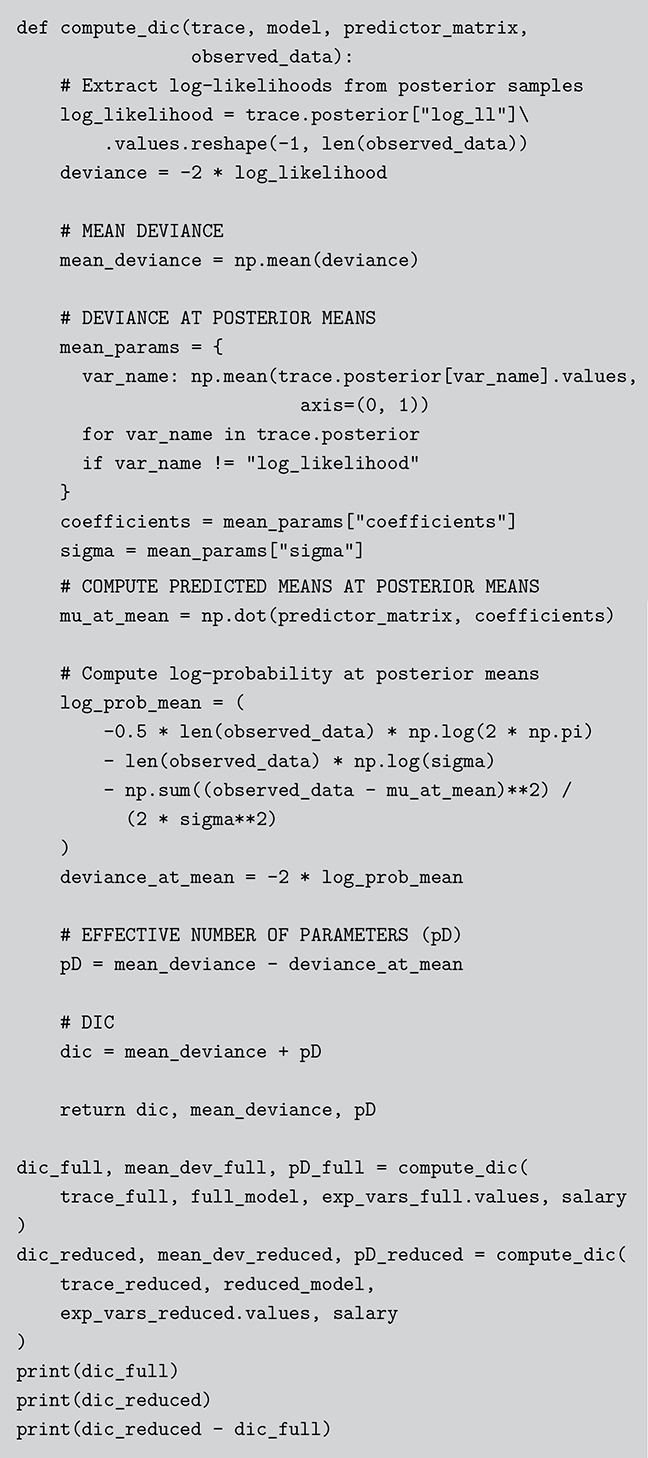
Code 1.036
 def compute_dic(trace, model, predictor_matrix,
 observed_data):
 # Extract log-likelihoods from posterior samples
 log_likelihood = trace.posterior["log_ll"]
 .values.reshape(-1, len(observed_data))
 deviance = -2 * log_likelihood
 # MEAN DEVIANCE
 mean_deviance = np.mean(deviance)
 # DEVIANCE AT POSTERIOR MEANS
 mean_params = {
 var_name: np.mean(trace.posterior[var_name].values,
 axis=(0, 1))
 for var_name in trace.posterior
 if var_name != "log_likelihood"
 }
 coefficients = mean_params["coefficients"]
 sigma = mean_params["sigma"]
 84# COMPUTE PREDICTED MEANS AT POSTERIOR MEANS
 mu_at_mean = np.dot(predictor_matrix, coefficients)
 # Compute log-probability at posterior means
 log_prob_mean = (
 -0.5 * len(observed_data) * np.log(2 * np.pi)
 - len(observed_data) * np.log(sigma)
 - np.sum((observed_data - mu_at_mean)**2) /
 (2 * sigma**2)
 )
 deviance_at_mean = -2 * log_prob_mean
 # EFFECTIVE NUMBER OF PARAMETERS (pD)
 pD = mean_deviance - deviance_at_mean
 # DIC
 dic = mean_deviance + pD
 return dic, mean_deviance, pD
 dic_full, mean_dev_full, pD_full = compute_dic(
 trace_full, full_model, exp_vars_full.values, salary
 )
 dic_reduced, mean_dev_reduced, pD_reduced = compute_dic(
 trace_reduced, reduced_model,
 exp_vars_reduced.values, salary
 )
 print(dic_full)
 print(dic_reduced)
 print(dic_reduced - dic_full)
Aligning with the Bayes Factor results, the difference in DIC between the two models is substantial, with a value of around -180. This strongly supports the full model over the reduced model, as a lower DIC indicates a better balance between model fit and complexity.
While DIC is highly useful, it should be noted there are some concerns with the use of the DIC. First, DIC is not invariant to reparameterizations of the parameters. Changes in parameterization can lead to significant differences in DIC values, which means that large changes in DIC need to be interpreted cautiously, especially when they result solely from parameterizations. Second, DIC comparisons are most effective when the form of the likelihood functions is the same across models, and only the explanatory variables differ. Likelihood functions from hierarchical models with different level structures can lead to difficult interpretational problems.
8.1.3 Posterior Predictive Checks
Using the posterior predictive distribution, multiple draws can be made to form a simulated dataset. By generating these replicated datasets, we can visually and statistically compare the distributional properties of the replicated data to those from the observed data. If the replicated data display significant differences in distributional qualities compared to the observed data, this suggests a poor fitting model. Additionally, the posterior predictive distribution is useful for making explicit model comparisons. By comparing the posterior predictive distributions of different candidate models, researchers can evaluate which model better captures the underlying data-generating process.
As an example, we can perform posterior predictive checks for the linear models of the Stack Overflow developers’ salaries from Section 6. The goal is to assess how well our Bayesian linear regression model fits the observed data by comparing the observed salaries to the predicted salaries generated from the posterior predictive distributions of the model. Since the MCMC sampler is a simulation process, generating posterior predictive distributions for new data points is very straightforward. By drawing from the posterior distributions of the model parameters at each iteration of the MCMC process, we can easily simulate new data points that reflect the uncertainty and variability captured by the model. In the following JAGS code, we use salary_pred[i]  dnorm(mu[i], tau) to simulate the new values for the outcome variable salary. In PyMC it’s even more straightforward with defined model context where we can simply use sample_posterior_predictive() to draw posterior predictive distributions with the same model context from the code in Section 6.
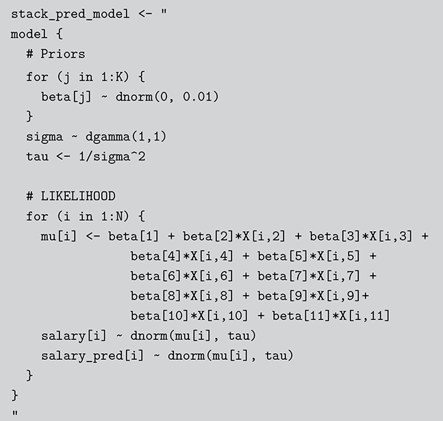
Code 1.037
 stack_pred_model <- "
 model {
 # Priors
 86for (j in 1:K) {
 beta[j]   dnorm(0, 0.01)
 }
 sigma   dgamma(1,1)
 tau <- 1/sigma^2
 # LIKELIHOOD
 for (i in 1:N) {
 mu[i] <- beta[1] + beta[2]*X[i,2] + beta[3]*X[i,3] +
 beta[4]*X[i,4] + beta[5]*X[i,5] +
 beta[6]*X[i,6] + beta[7]*X[i,7] +
 beta[8]*X[i,8] + beta[9]*X[i,9]+
 beta[10]*X[i,10] + beta[11]*X[i,11]
 salary[i]   dnorm(mu[i], tau)
 salary_pred[i]   dnorm(mu[i], tau)
 }
 }
 "
Code 1.038
 with model:
 stack_ppc = pm.sample_posterior_predictive(
 stack_mcmc,
 var_names=["salary_obs"],
 random_seed=526)
Once we obtain the posterior predictive distributions, we can check for alignment or discrepancies between the simulated posterior predictive distributions and the observed data. For example, in Figure 7, we overlay the density lines of the simulated posterior predictive distributions on the histogram of observed outcomes. To interpret the posterior predictive checks, we look for a close alignment between the observed data and the simulated values. If the model is a good fit, the simulated distributions should closely follow the shape, spread, and central tendency of the observed data. Significant deviations between the observed and predicted distributions can indicate potential issues with the model.
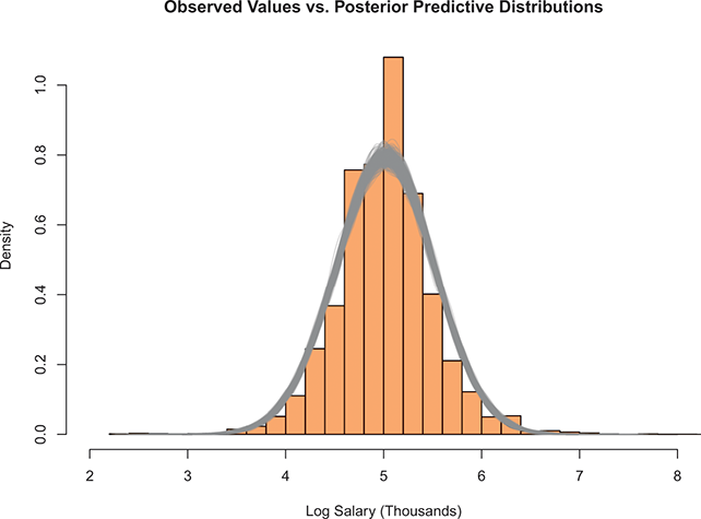
Figure 7 Comparing Observed Values and Posterior Predictive Distributions
Figure 7Long description
This figure displays a comparison between observed data and posterior predictive distributions for log-transformed salary measured in thousands. The horizontal axis is labeled Log Salary (Thousands) and ranges approximately from 2 to 8. The vertical axis shows density values from 0 to 1. The orange histogram bars represent the observed values of log salary, clustered prominently around the center value of 5. Superimposed on this histogram is a smooth gray curve, which represents the posterior predictive distribution. The close alignment of the gray curve with the orange bars indicates that the posterior model fits the observed data well.
To formally assess model fit, we can also define a test quantity  that summarizes the specific aspects of the data, such as the mean, variance, or quantiles. By comparing the observed test quantities
  to the distribution of test quantities
  ) from the predicted data, we can evaluate how well the model reproduces the data. For example, we can use the posterior predictive p-value to measure the probability that the test statistic for the replicated data is more extreme than for the observed data:
  (Meng, Reference Meng1994). The following R and Python code blocks calculate the posterior predictive probability for the Stack Overflow developers’ salary example.
Code 1.039
 # OBSERVED AND POSTERIOR PREDICTIVE OUTCOMES
 observed <- log(stack$ConvertedCompYearly)
 pred_salary <- chain1[,13:ncol(chain1)-1]
 # OBSERVED AND POSTERIOR PREDICTIVE MEANS
 observed_test_stat <- mean(observed)
 replicated_test_stats <- apply(pred_salary, 1, mean)
 88(p_value
 <- mean(replicated_test_stats >= observed_test_stat))
Code 1.040
 # OBSERVED AND POSTERIOR PREDICTIVE OUTCOMES
 observed_salary
 = np.log(stack[’ConvertedCompYearly’].values)
 pred_salary = stack_ppc["posterior_predictive"] \
 ["salary_obs"].stack(samples=("chain", "draw")).values
 # OBSERVED AND POSTERIOR PREDICTIVE MEANS
 observed_test_stat = np.mean(observed_salary)
 pred_test_stat = np.mean(pred_salary, axis=1)
 p_value = np.mean(pred_test_stat >= observed_test_stat)
 print(p_value)
8.2 Common Convergence Diagnostics
Convergence is a crucial aspect of Markov Chain Monte Carlo (MCMC) methods, ensuring that the posterior samples generated accurately represent the target posterior distribution. As shown in Section 4, the results from an MCMC posterior sample are not deemed reliable until the chain has reached its steady state (stationary) distribution and completely mixed through the parameter space. Convergence means the sample distribution has stabilized and draws from the true posterior distribution, indicating that the chain has moved beyond the initial non-converged phase. While there are different approaches to checking convergence, such as theoretical analysis, in-progress monitoring, and perfect sampling (see Gill, Reference Gill2014, p.479–480 for more details), the general process involves running the chain for a sufficiently large number of iterations, discarding a large proportion of the initial values (e.g., the first half), and then checking the remaining distribution using both numerical and graphical methods. It is essential to remember that convergence diagnostics are indicators of nonconvergence: failing to find evidence of nonconvergence does not directly confirm convergence. Therefore, a careful practitioner should use multiple diagnostics to assess a single Markov chain, as any one diagnostic can provide sufficient evidence of failure.
8.2.1 Trace Plots
One straightforward way to check convergence is by examining the posterior distributions graphically. A common graphical method is the trace plot, which displays the sampled parameter values over iterations. A converged and well-mixing chain should exhibit random fluctuations around a stable mean, forming a “fuzzy caterpillar” pattern without trends or periodic patterns. This implies that the chain is thoroughly exploring the parameter space and has likely reached its stationary distribution. If the trace plot shows trends, drifts, or periodicity, it suggests that the chain has not yet converged, and additional iterations are necessary. We do so here to produce Figure 8 from the Stack Overflow model.
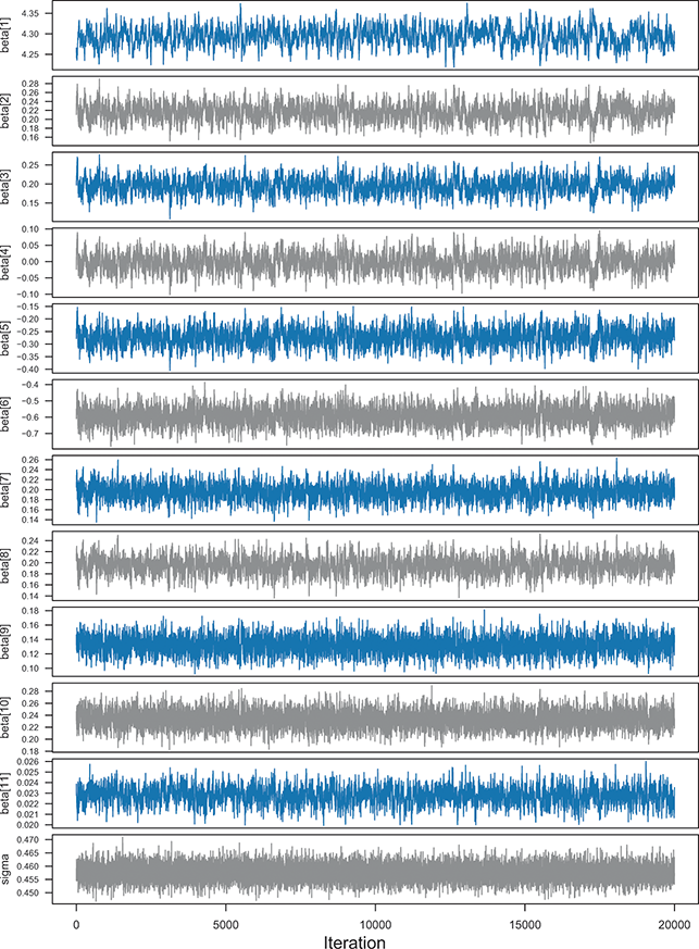
Figure 8 Trace Plot for Posterior Samples of the Stack Overflow Example
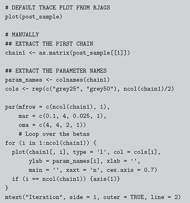
Code 1.041
 # DEFAULT TRACE PLOT FROM RJAGS
 plot(post_sample)
 # MANUALLY
 ## EXTRACT THE FIRST CHAIN
 chain1 <- as.matrix(post_sample[[1]])
 ## EXTRACT THE PARAMETER NAMES
 param_names <- colnames(chain1)
 cols <- rep(c("grey25", "grey50"), ncol(chain1)/2)
 par(mfrow = c(ncol(chain1), 1),
 mar = c(0.1, 4, 0.025, 1),
 oma = c(4, 4, 2, 1))
 # Loop over the betas
 for (i in 1:ncol(chain1)) {
 plot(chain1[, i], type = ’l’, col = cols[i],
 ylab = param_names[i], xlab = ”,
 main = ”, xaxt = ʼn’, cex.axis = 0.7)
 if (i == ncol(chain1)) axis(1)
 }
 mtext("Iteration", side = 1, outer = TRUE, line = 2)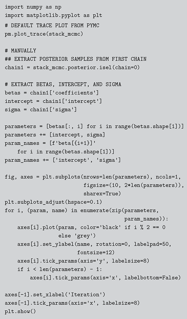
Code 1.042
 import numpy as np
 import matplotlib.pyplot as plt
 91# DEFAULT TRACE PLOT FROM PYMC
 pm.plot_trace(stack_mcmc)
 # MANUALLY
 ## EXTRACT POSTERIOR SAMPLES FROM FIRST CHAIN
 chain1 = stack_mcmc.posterior.isel(chain=0)
 # EXTRACT BETAS, INTERCEPT, AND SIGMA
 betas = chain1[’coefficients’]
 intercept = chain1[’intercept’]
 sigma = chain1[’sigma’]
 parameters = [betas[:, i] for i in range(betas.shape[1])]
 parameters += [intercept, sigma]
 param_names = [f’beta[i+1]’
 for i in range(betas.shape[1])]
 param_names += [’intercept’, ’sigma’]
 fig, axes = plt.subplots(nrows=len(parameters), ncols=1,
 figsize=(10, 2*len(parameters)),
 sharex=True)
 plt.subplots_adjust(hspace=0.1)
 for i, (param, name) in enumerate(zip(parameters,
 param_names)):
 axes[i].plot(param, color=’black’ if i % 2 == 0
 else ’grey’)
 axes[i].set_ylabel(name, rotation=0, labelpad=50,
 fontsize=12)
 axes[i].tick_params(axis=’y’, labelsize=8)
 if i < len(parameters) - 1:
 axes[i].tick_params(axis=’x’, labelbottom=False)
 axes[-1].set_xlabel(’Iteration’)
 axes[-1].tick_params(axis=’x’, labelsize=8)
 plt.show()
Figure 8 shows that the chains display random fluctuations around a stable mean without clear trends or drifts. This indicates good mixing, meaning the chains have likely reached the stationary distribution after exploring the parameter space effectively. If we saw for some parameters the chains exhibit slow movement and larger shifts over time, it can suggest that the model may not have fully converged. It’s recommended to run additional iterations or apply other diagnostic methods, or the model may require re-parameterization for better mixing.
We show in the preceding code how to pull up information from MCMC chains to manually create a trace plot. MCMC packages usually include default plotting functions for trace plot. In R, we can apply the plot.mcmc() function from the coda package on an MCMC output object, and it will automatically create the trace plot for all parameters. In Python, we can use the plot_trace() function from the PyMC library to achieve the same purpose.
8.2.2 Geweke Convergence Diagnostic
For formal, mathematical methods, the most common empirical diagnostics operate on marginal distributions individually and indicate when a single dimension chain is sufficiently trending as to violate specified distributional assumptions that are implied under the assumption of stability. Or diagnostics can check for consistency across multiple chains if they are sampled from the same target distributions. To demonstrate the need for an empirical diagnostic for purely discrete parameters we quickly review the four most common formal tests for assessing convergence. These are provided in the coda and boa packanges in R, and on the dedication Github page for this text in Python. For more details, see Gill (Reference Gill2014). For a review of other diagnostics, see Brooks & Roberts (1998) or Cowles & Carlin (1996). In R we make use of the coda package, which contains these functions. For Python we have provided code in the dedicated Github page for this work.
The Geweke diagnostic (Geweke, Reference Geweke1992) preselects for the  th model parameter two nonoverlapping window proportions of the full chain. The first window is early in the saved runs and is of length
  ,
,  , while the second is from later in the chain and is of length
  ,
,  . For each of these, calculate the mean,
  and
and  , the statistic
  is defined as
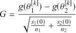
where  and
and  are the symmetric spectral density functions (the time-series equivalent of the standard deviation). This test statistic is asymptotically standard normal. Therefore, large values of
  indicate a difference in the chain between the two windows and therefore provide evidence of nonconvergence. The software packages implement the Geweke diagnostic by calculating the sample mean and z-scores of the difference between two segments, by default usually 10% from the initial segments of the chain and the last 50% of the remaining chain. If the chain has converged, the majority of these
  -scores should fall within 1.96 standard deviations of zero, corresponding to a 0.05 significance level.
The following code uses the geweke.diag() function from the coda package to employ Geweke diagnostics in R. We can also set the fractions of the MCMC chain for the two segments. Output 8.2.2 shows the test statistics for the linear model from the Stack Overflow example. The results indicate that with the posterior samples for all parameters there is no evidence of nonconvergence since all the  -scores are within 1.96 standard deviations of zero.

Code 1.043
 library(coda)
 geweke.diag(post_sample[[1]], frac1=0.1, frac2=0.5)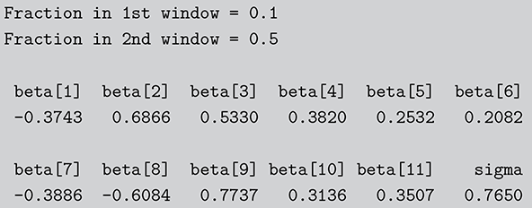
Code 1.044
 Fraction in 1st window = 0.1
 Fraction in 2nd window = 0.5
 beta[1] beta[2] beta[3] beta[4] beta[5] beta[6]
 -0.3743 0.6866 0.5330 0.3820 0.2532 0.2082
 beta[7] beta[8] beta[9] beta[10] beta[11] sigma
 -0.3886 -0.6084 0.7737 0.3136 0.3507 0.7650
Code 1.045
 chain1 = stack_mcmc.posterior.isel(chain=0)
 geweke_results = geweke_diag(chain1,first=0.1, last=0.5)
 print(geweke_results)
8.2.3 Heidelberger & Welch Convergence Diagnostic
The Heidelberger & Welch diagnostic (Heidelberger & Welch, Reference Heidelberger and Welch1983) assesses the convergence of Markov chains by analyzing the stability of their cumulative sums. Define  as the length of the chain after burn-in,
  as the test chain proportion,
 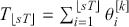 as the sum of the chain values from one to the integer value just below
  ,
,  as the chain mean times the integer value just below
  , and
, and  as the spectral density of the chain. A Cramér–Von Mises test statistic (which measures the discrepancy between the empirical and theoretical cumulative distribution functions) for sums as cumulative values scaled by the spectral density, for any given
  , is
, is
This statistic measures the deviation of the cumulative sum of the chain values from the expected sum, scaled by the spectral density. Similar to the Geweke test, the Heidelberger & Welch diagnostic is based on the principle of asymptotic normality. Large values of  indicate significant deviations, suggesting that the chain has not yet converged.
The heidel.diag function in R implements a stationarity test by successively discarding increasing portions of the chain until the null hypothesis is accepted or 50% is discarded. Additionally, it also conducts a half-width test that calculates a 95% confidence interval for the mean using the portion of the chain that passed the stationarity test. If the ratio between the half-width and the mean is lower than a specified threshold (‘eps’), the half-width test is passed. In what follows we apply the Heidelberger & Welch diagnostic in both R and Python:

Code 1.046
heidel.diag(post_sample[[1]])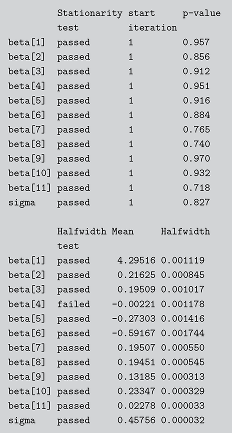
Code 1.047
 Stationarity start p-value
 test iteration
 beta[1] passed 1 0.957
 beta[2] passed 1 0.856
 beta[3] passed 1 0.912
 95beta[4] passed 1 0.951
 beta[5] passed 1 0.916
 beta[6] passed 1 0.884
 beta[7] passed 1 0.765
 beta[8] passed 1 0.740
 beta[9] passed 1 0.970
 beta[10] passed 1 0.932
 beta[11] passed 1 0.718
 sigma passed 1 0.827
 Halfwidth Mean Halfwidth
 test
 beta[1] passed 4.29516 0.001119
 beta[2] passed 0.21625 0.000845
 beta[3] passed 0.19509 0.001017
 beta[4] failed -0.00221 0.001178
 beta[5] passed -0.27303 0.001416
 beta[6] passed -0.59167 0.001744
 beta[7] passed 0.19507 0.000550
 beta[8] passed 0.19451 0.000545
 beta[9] passed 0.13185 0.000313
 beta[10] passed 0.23347 0.000329
 beta[11] passed 0.02278 0.000033
 sigma passed 0.45756 0.000032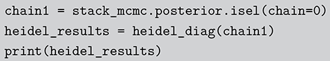
Code 1.048
 chain1 = stack_mcmc.posterior.isel(chain=0)
 heidel_results = heidel_diag(chain1)
 print(heidel_results)
The Heidelberger & Welch diagnostic results show that all parameters passed the stationarity test starting from the first iteration. This indicates that, from the very beginning of the saved chain, the parameters show no significant signs of drift or trends and have reached their stationary distribution. Most parameters pass the halfwidth test excepf for  . This means that the precision of the mean estimates of parameters are satisfactory based on the required confidence intervals. The halfwidths are small relative to the means, which implies that the chains have run long enough to provide reliable estimates. For
  , the failure can indicate insufficient posterior sample size or slow mixing in the chain. More iterations or thinning may be required for this parameter.
8.2.4 Brooks, Gelman, & Rubin Convergence Diagnostic
The Brooks, Gelman, & Rubin diagnostic (Gelman & Rubin, Reference Gelman and Rubin1992; Brooks & Gelman, Reference Brooks and Gelman1998) is based on an analysis of variance comparison of parallel runs of a Markov chain started from overdispersed positions. To perform this diagnostic, run  chains of length
  from these starting points discarding the first
  , and for the
  th parameter of the model, denote
  as the
  th value (
 ) from the
  th parallel chain (
 ). Calculate two variances:
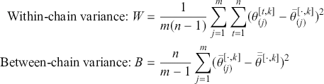
Now the marginal posterior variance is  , and the “scale reduction factor” is:
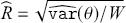
given by:
 (8.13)
where  is the posterior distribution of
  after observing the data
  . The last expression comes from the assumption that
  and
and  are independent. The posterior predictive distribution is the product of the single-variable PDF or PMF
  and the posterior distribution
  , integrated over the uncertainty in
  . This results in a probability statement of
  that depends only on the observed data
  .
.
The following code produces the Brooks, Gelman, & Rubin diagnostic in R and Python. The potential scale reduction factor is calculated for each variable. All the parameters have a potential scale reduction factor point estimate of 1. This means that the within-chain and between-chain variances are virtually identical, suggesting that all chains have converged. The upper confidence intervals for all parameters are also 1, which further confirms that the chains have likely converged. In practice, upper confidence intervals below 1.1 are generally acceptable.

Code 1.049
gelman.diag(post_sample)
Code 1.050
Potential scale reduction factors: Point est. Upper C.I. beta[1] 1 1 beta[2] 1 1 beta[3] 1 1 beta[4] 1 1 beta[5] 1 1 beta[6] 1 1 beta[7] 1 1 beta[8] 1 1 beta[9] 1 1 beta[10] 1 1 beta[11] 1 1 sigma 1 1
Code 1.051
 gelman_results = gelman_rubin(stack_mcmc.posterior)
 print(gelman_results)
In R, we can also make use of the package superdiag that offers a comprehensive set of tools for convergence diagnostics, including methods like Gelman-Rubin, Geweke, Heidelberger–Welch, Raftery–Lewis, and the Hellinger distance. It also includes plotting functions for trace plots and density histograms. One of the strengths of superdiag is its ability to present all diagnostic statistics and graphical outputs at once, making it convenient to assess MCMC convergence.
8.3 Computing Quantities of Interest and Their Uncertainty Using Posterior Distributions
Simulations have been demonstrated to be very versatile and effective in addressing the uncertainty of model parameters (King, Tomz, & Wittenberg, Reference King, Tomz and Wittenberg2000). As a simulation-based method, Bayesian analysis with MCMC provides an even more holistic approach, allowing us to leverage the full posterior distributions of model parameters to estimate quantities of interest and their uncertainty. In this section, we demonstrate how we can use posterior distributions to evaluate a variety of model statistics (Murr, Traunmüller, & Gill, Reference Murr, Traunmüller and Gill2023).
For regression models, we often want to evaluate which explanatory variables are most influential in explaining the variations of the outcome variable, in other words effect size. While conventional approaches allow us to compare point estimates, they do not straightforwardly address the uncertainty of these effect sizes. In Bayesian analysis, we can leverage the full posterior distribution to compute the probability that the effect size of one parameter is larger than that of others. Specifically, for any two parameters  and
and  , this probability can be computed as follows:

where  equals 1 if the condition inside is true and 0 otherwise. By doing this, we can obtain the relative importance of coefficients. To find the most important variable, we compute the probability that each coefficient has the largest absolute coefficient across all variables:

In the following, we compute the probability of which absolute coefficient is largest for the developer’s salary analysis from Section 6.

Code 1.052
 # CONVERT THE MCMC OUTPUT TO A MATRIX
 mcmc_mat <- as.matrix(post_sample[[1]])
 # EXTRACT THE SELECTED BETA COEFFICIENTS
 beta_samples <- post_matrix[, c("beta[2]","beta[3]",
 "beta[7]","beta[8]","beta[9]","beta[10]",
 "beta[11]")]
 99# CALCULATE PROBABILITY OF EACH BETA BEING THE LARGEST
 apply(beta_samples, 2, function(beta_col) {
 mean(abs(beta_col) == apply(abs(beta_samples), 1, max))
 })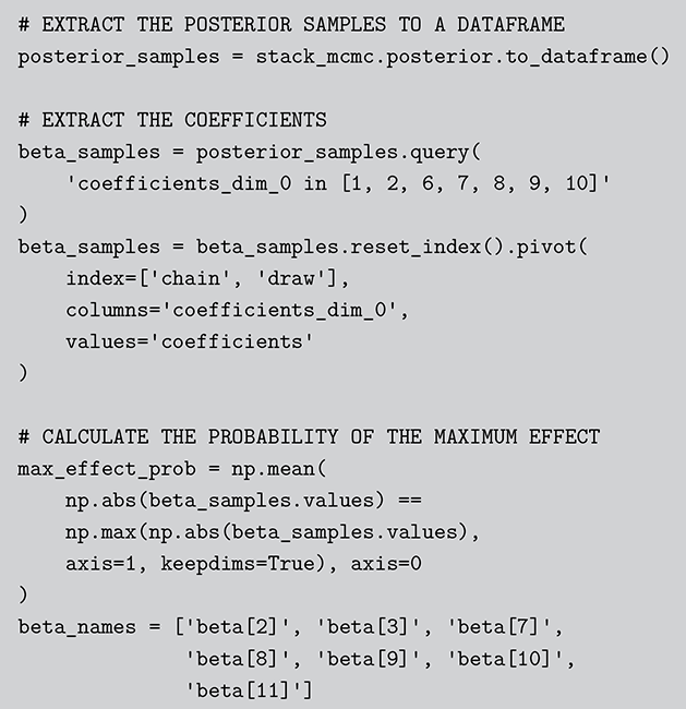
Code 1.053
 # EXTRACT THE POSTERIOR SAMPLES TO A DATAFRAME
 posterior_samples = stack_mcmc.posterior.to_dataframe()
 # EXTRACT THE COEFFICIENTS
 beta_samples = posterior_samples.query(
 ’coefficients_dim_0 in [1, 2, 6, 7, 8, 9, 10]’
 )
 beta_samples = beta_samples.reset_index().pivot(
 index=[’chain’, ’draw’],
 columns=’coefficients_dim_0’,
 values=’coefficients’
 )
 # CALCULATE THE PROBABILITY OF THE MAXIMUM EFFECT
 max_effect_prob = np.mean(
 np.abs(beta_samples.values) ==
 np.max(np.abs(beta_samples.values),
 axis=1, keepdims=True), axis=0
 )
 beta_names = [’beta[2]’, ’beta[3]’, ’beta[7]’,
 ’beta[8]’, ’beta[9]’, ’beta[10]’,
 ’beta[11]’]
Marginal effects measure the change in the expected value of the outcome variable with a one-unit change in a predictor variable, holding other variables constant. In a Bayesian context, these effects can be derived from the posterior distribution of the model parameters, providing a full probabilistic description. In the context of linear models, marginal effects are straightforward as they correspond directly to the regression coefficients. In logistic regression, marginal effects are more informative as they represent the change in the predicted probability of the outcome for a one-unit change in the predictor. When evaluating marginal effects, estimating them at mean values can be less meaningful, especially when variables are binary or have a wide range of values.
Using the local anti-immigrant ordinance data from Section 7 as an example, we may hypothesize that the effects of the changes in the percent of immigrants from 1990 to 2000 are not constant. These effects may be particularly pronounced when the flow of immigrants starts. For instance, an initial increase in the percentage of immigrants might have the most significant effect, but this impact could diminish once the immigrants are integrated into the community. We can compute the marginal effects and associated uncertainty from the posterior distribution. The following blocks of R and Python code calculate the marginal effects based on the model in Section 7.2. Figure 9 plots the marginal effects with 95% HPD intervals for the changes in the percentage of immigrants in the 1990s.

Figure 9 Marginal Effects of Changes in percent of Immigrants
Figure 9Long description
The x-axis represents the change in percentage of immigrants, ranging from approximately negative 0.1 to 0.3. The y-axis represents the marginal effect, ranging from 0 to 5. A smooth blue line indicates the estimated marginal effect, which begins at about 2.5 when the change is near 0 and initially rises slightly before declining steadily as the percentage increases. The gray vertical bars around the line represent the ninety five percent credible intervals, showing the uncertainty around the estimates. The intervals are widest at lower percentage changes and narrow as the percentage increases.
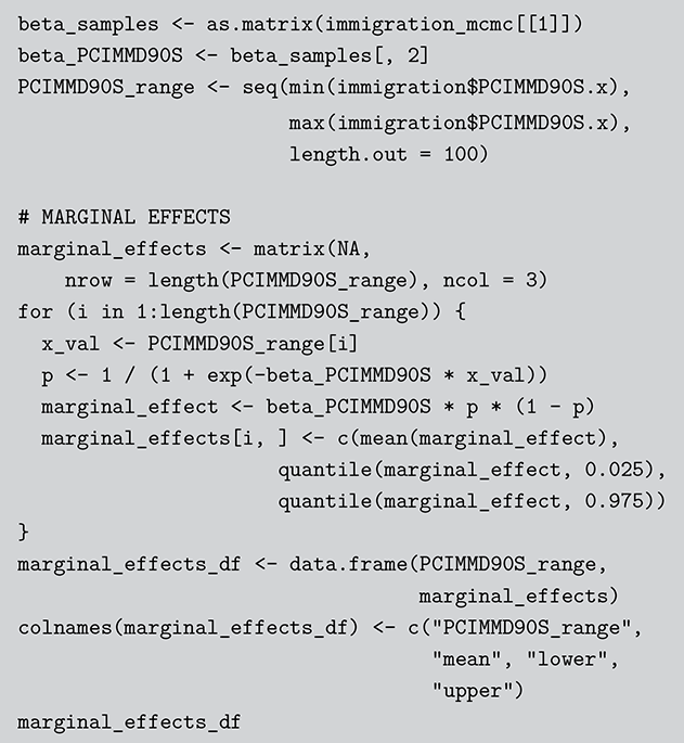
Code 1.054
 beta_samples <- as.matrix(immigration_mcmc[[1]])
 beta_PCIMMD90S <- beta_samples[, 2]
 PCIMMD90S_range <- seq(min(immigration$PCIMMD90S.x),
 101max(immigration$PCIMMD90S.x),
 length.out = 100)
 # MARGINAL EFFECTS
 marginal_effects <- matrix(NA,
 nrow = length(PCIMMD90S_range), ncol = 3)
 for (i in 1:length(PCIMMD90S_range)) {
 x_val <- PCIMMD90S_range[i]
 p <- 1 / (1 + exp(-beta_PCIMMD90S * x_val))
 marginal_effect <- beta_PCIMMD90S * p * (1 - p)
 marginal_effects[i, ] <- c(mean(marginal_effect),
 quantile(marginal_effect, 0.025),
 quantile(marginal_effect, 0.975))
 }
 marginal_effects_df <- data.frame(PCIMMD90S_range,
 marginal_effects)
 colnames(marginal_effects_df) <- c("PCIMMD90S_range",
 "mean", "lower",
 "upper")
 marginal_effects_df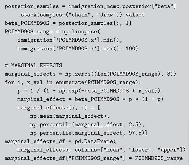
Code 1.055
 posterior_samples = immigration_mcmc.posterior["beta"]
 .stack(samples=("chain", "draw")).values
 beta_PCIMMD90S = posterior_samples[:, 1]
 PCIMMD90S_range = np.linspace(
 immigration[’PCIMMD90S.x’].min(),
 immigration[’PCIMMD90S.x’].max(), 100)
 # MARGINAL EFFECTS
 marginal_effects = np.zeros((len(PCIMMD90S_range), 3))
 for i, x_val in enumerate(PCIMMD90S_range):
 p = 1 / (1 + np.exp(-beta_PCIMMD90S * x_val))
 marginal_effect = beta_PCIMMD90S * p * (1 - p)
 marginal_effects[i, :] = [
 np.mean(marginal_effect),
 102np.percentile(marginal_effect, 2.5),
 np.percentile(marginal_effect, 97.5)]
 marginal_effects_df = pd.DataFrame(
 marginal_effects, columns=["mean", "lower", "upper"])
 marginal_effects_df["PCIMMD90S_range"] = PCIMMD90S_range
The classical  is calculated as the proportion of variance explained by the model, obtained by subtracting the residual variance from the total variance and dividing by the total variance,
  . While this can be a handy summary of the model fit, it has two issues from a Bayesian perspective. First, it usually does not account for the uncertainty of the parameters. Second, with strong priors and weak data the classical
  can be greater than 1. To address these issues, Gelman et al. (Reference Gelman, Goodrich, Gabry and Vehtari2019) propose an alternative Bayesian
  , which can be computed based on the posterior samples and account for the posterior uncertainty in the parameters. It is calculated using the posterior distributions of the predicted values and the associated residuals:
where  represents the sample variance,
  .
.  is the variance of the predicted values.
  is the expected residual variance.
We can build upon the posterior predictive distribution from Section 8.1.3 and compute Bayesian  in R and Python as follows:


Code 1.056
 observed <- log(stack$ConvertedCompYearly)
 residuals <- sweep(pred_salary, 2, observed)
 var_y <- var(observed)
 var_pred <- apply(pred_salary, 1, var)
 var_resid <- apply(residuals, 1, var)
 bayesian_r2 <- var_pred / (var_pred + var_resid)
 (bayesian_r2_mean <- mean(bayesian_r2))
 (bayesian_r2_ci <- quantile(bayesian_r2,c(0.025, 0.975)))

Code 1.057
 pred_salary = stack_ppc["posterior_predictive"]
 ["salary_obs"].stack(samples=("chain", "draw")).values
 observed_salary
 = np.log(stack[’ConvertedCompYearly’].values)
 mean_pred_salary = np.mean(pred_salary, axis=1)
 residuals = observed_salary - mean_pred_salary
 var_y = np.var(observed_salary)
 var_pred = np.var(pred_salary, axis=0)
 var_resid = np.var(residuals)
 bayesian_r2 = var_pred / (var_pred + var_resid)
 bayesian_r2_mean = np.mean(bayesian_r2)
 bayesian_r2_ci = np.percentile(bayesian_r2, [2.5, 97.5])
This section has covered the key practical considerations that follow Bayesian estimation via MCMC – model comparison, convergence diagnostics, and the use of posterior simulations to summarize uncertainty and evaluate fit. From the foundational principles of Bayesian inference, through the development of Monte Carlo methods and Markov chains, to building and estimating regression models, we now complete the core workflow of Bayesian analysis.
9 Final Remarks
In this Element, we have focused on foundational Bayesian regression models and their implementation using R and Python. We also covered Markov Chain Monte Carlo (MCMC) methods, which are essential for estimating Bayesian models. While these topics form the backbone of practical Bayesian inference, it’s important to note that Bayesian methods are far more powerful than we could cover in this Element.
One of the key strengths of the Bayesian framework is its capacity to adapt to more advanced and complex modeling scenarios. As we demonstrated in the book, the Bayesian framework can be straightforwardly extended to different types of models, offering a coherent way to model uncertainty and provide probabilistic inferences about different parameters. Furthermore, Bayesian methods are very capable of handling dependence in data structure. This is particularly useful for time series, spatial, and network data. The extension of Bayesian models can provide a flexible framework to model complex dependencies while incorporating uncertainty in both parameters and data-generating processes. Hierarchical models, in particular, fit seamlessly within the Bayesian framework, allowing us to account for multilevel variation and partial pooling of information across groups. In addition, Bayesian methods are also well-suited for nonparametric modeling, which offers even more flexibility by allowing the model to grow in complexity with the data. Approaches like Gaussian processes and Dirichlet process mixtures enable Bayesian nonparametric inference, where the model structure is not fixed but can adapt to reveal hidden patterns in the data. This flexibility is invaluable in settings where the true underlying process is unknown or difficult to specify, making nonparametric Bayesian models particularly powerful in applications such as machine learning, clustering, and high-dimensional data analysis.
On the software front, we used JAGS and PyMC as tools to explicitly teach Bayesian model specification. These platforms are excellent for understanding the basic structure of Bayesian models, offering accessible ways to define and fit models using widely used MCMC samplers like Gibbs sampling and Hamiltonian Monte Carlo. They also serve as great gateways to other MCMC and probabilistic programming tools, such as STAN, TensorFlow Probability, and JAX. These tools offer additional advantages, including more efficient, scalable, and robust sampling methods. In particular, TensorFlow Probability and JAX are well suited for applying Bayesian methods to high-dimensional data and machine learning, leveraging modern computational architectures like GPUs and TPUs.
While this Element introduces some of the fundamental methodology and tools for Bayesian modeling, there remains a wealth of methods and techniques to explore. Readers are encouraged to build on what they have learned here by applying Bayesian methods to new problems, experimenting with a range of tools, and exploring approaches to their own research. The flexibility of Bayesian analysis offers endless opportunities for further learning and discovery across a wide range of applications.
California Institute of Technology
R. Michael Alvarez has taught at the California Institute of Technology his entire career, focusing on elections, voting behavior, election technology, and research methodologies. He has written or edited a number of books (recently, Computational Social Science: Discovery and Prediction, and Evaluating Elections: A Handbook of Methods and Standards) and numerous academic articles and reports.
Washington University in St. Louis
Betsy Sinclair is Professor and Chair of Political Science at WashU. Her research focuses on social influence and American political behavior. She is a fellow of the Society of Political Methodology and has served as an associate editor of Political Analysis and in leadership roles in The Society of Political Methodology and Visions in Political Methodology.
About the Series
The Elements Series Quantitative and Computational Methods for the Social Sciences contains short introductions and hands-on tutorials to innovative methodologies. These are often so new that they have no textbook treatment or no detailed treatment on how the method is used in practice. Among emerging areas of interest for social scientists, the series presents machine learning methods, the use of new technologies for the collection of data and new techniques for assessing causality with experimental and quasi-experimental data.