

Introduction
Dust on glacier surfaces is a controlling factor of ice albedo and imparts significant influence on ablation rates, surface water volumes and supraglacial weathering crust development (e.g. Reference Cutler and MunroCutler and Munro, 1996; Reference Adhikary, Nakawo, Seko and ShakyaAdhikary and others, 2000). Surface dust frequently comprises significant quantities of organic material, algae and bacteria (Reference Takeuchi, Kohshima and SekoTakeuchi and others, 2001; Reference HodsonHodson and others, 2008). Biological activity binds organic and inorganic material together in characteristically small (typically <1 cm) aggregate granules (Reference Takeuchi, Kohshima and SekoTakeuchi and others, 2001; Reference TakeuchiTakeuchi, 2002). This biogenic dust is commonly termed cryoconite. The presence of low-albedo humic substances in cryoconite further reduces the overall mineral dust albedo (e.g. Reference Takeuchi, Kohshima and SekoTakeuchi and others, 2001; Reference TakeuchiTakeuchi, 2002, Reference Takeuchi2009; Reference Takeuchi and LiTakeuchi and Li, 2008). Consequently, cryoconite deserves increased research attention because its presence enhances ice melting and wastage over a range of spatial scales from valley glaciers to ice sheets (e.g. Reference Kohshima, Seko and YoshimuraKohshima and others, 1993; Reference BøggildBøggild, 1998; Reference Takeuchi, Kohshima and SekoTakeuchi and others, 2001; Reference Takeuchi and LiTakeuchi and Li, 2008; Reference Bøggild, Brandt, Brown and WarrenBøggild and others, 2010). The occurrence of cryoconite has potential impacts on supraglacial hydrological connections (Reference Fountain, Tranter, Nylen, Lewis and MuellerFountain and others, 2004; Reference Irvine-FynnIrvine-Fynn, 2008; Reference MacDonell and FitzsimonsMacDonell and Fitzsimons, 2008) and nutrient and carbon cycling (Reference Bagshaw, Tranter, Fountain, Welch, Basagi and LyonsBagshaw and others, 2007; Reference HodsonHodson and others, 2007, Reference Hodson2010) as well as influencing primary succession in deglaciating environments (e.g. Reference Kaštovská, Elster, Stibal and ŠantréčkováKaštovská and others, 2005).
Despite the growing research interest in cryoconite, there are few primary data available in key areas of interest (Reference TakeuchiTakeuchi, 2002; Reference HodsonHodson and others, 2007). These include quantitative assessment of the morphology and genesis of cryoconite granules in different glacial contexts, and the temporal variability of cryoconite extent and transport across the ice surface over spatial scales from centimetres to kilometres. Previous laboratory analysis of cryoconite granule geometry used digital images of cryoconite acquired through microscopy (Reference Takeuchi, Kohshima and SekoTakeuchi and others, 2001). Individual granule dimensions in each microscope image were measured manually using computer image-processing software (personal communication from N. Reference TakeuchiTakeuchi, 2009). In the field, an imaging approach was also proposed by Reference HodsonHodson and others (2007) using unmanned aerial vehicles (UAVs) supported by ground-truth surveys to quantify supraglacial cryoconite distribution. Both existing methodologies are limited in effectiveness by the requirement to use specialist equipment (e.g. microscopy, UAVs); the large number of raw data generated by high-resolution digital imaging; and a dependence on manual image processing and/or the use of proprietary (high-cost) software to perform supervised classification of image components (e.g. Reference HodsonHodson and others, 2007). Furthermore, UAV field data have relatively low spatial resolution and are subject to variable imaging geometries and lighting conditions.
Here, building upon the earlier work of Reference HodsonHodson and others (2007), we present a set of robust, semi-automated data-processing protocols to support increased use of low-cost imaging methodologies to collect primary datasets for (1) cryoconite granule morphology; (2) variation in spatial extent of supraglacial cryoconite over an altitude transect in the field; and (3) temporal variation in supraglacial cryoconite at a single location in the field. The datasets were acquired in Arctic settings exhibiting surface cryoconite forms, using standard commercial digital cameras and the protocols developed using public domain software. The aim of this work is to establish transferable, rapid measurement tools to make practical the collation of comparable, standardized datasets for cryoconite morphology and occurrence over a wide variety of glacial environments.
Materials and Methods
Cryoconite sources and sampling
Granule morphologic analysis (laboratory)
Cryoconite granules (Fig. 1a) were collected from Longyearbreen, Svalbard (78°10′49″ N, 15°30′21″ E), during a field campaign in summer 2008 (for details see Reference HodsonHodson and others, 2010). In the laboratory, samples were placed in water-filled glass Petri dishes overlying standard 2 mm square graph paper. Five granules in each dish were carefully isolated for analysis (Fig. 1a). Digital colour (redgreen-blue, RGB) images (uncompressed JPEG) were acquired using a 6.08-megapixel Fuji FinePix-S6500 camera mounted vertically above each Petri dish under standard room illumination with no flash.
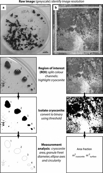
Fig. 1. Example images of (a) cryoconite granules and (b) in situ extent as used in analyses presented here, schematically illustrated in sequence.
Field analysis of spatial variability in supraglacial cryoconite extent
Supraglacial cryoconite coverage over a transect at the margin of the Greenland ice sheet (GrIS), at a site near Kangerlussuaq (67°09′05″ N, 98°01′16″ W), was investigated using image acquisition methods similar to those detailed in Reference HodsonHodson and others (2007). Digital colour images (uncompressed JPEG) were acquired from ∼1.5 m above the ice surface with 1.92-megapixel (1600 × 1200) images captured using a Fuji FinePix-S6500 camera and a field of view encompassing a 40 × 40 cm quadrat placed on the ice (Fig. 1b). Between 16 and 50 images were taken in a grid formation at each of seven survey locations (250 images in total) spanning a 70 m elevation range over the period 28–30 August 2008.
Field analysis of temporal variation in supraglacial cryoconite extent
A time-lapse sequence of 216 images was collected at a single point on the ice surface at hourly intervals over a period of 9 days (20–29 July) at Longyearbreen, Svalbard (78°10′49″ N, 15°30′21″ E) in summer 2008. The site was considered to be typical of ablating glacier ice exhibiting an irregular, time-variable surface texture, pitted with numerous small (centimetre-scale) cryoconite holes. Digital colour images (uncompressed JPEG) were captured using a 7.08-megapixel (3072 × 2304) Pentax Optio WP30 digital camera. The camera was fixed to a vertical pole drilled and frozen into the glacier ice and remained immobile as the ice surface ablated around the mount. The distance from the camera to the ice surface increased from 0.5 m to ∼1.0 m over the imaging period. A subset of these data and field site details are presented in Reference HodsonHodson and others (2010).
Digital image processing
ImageJ software
All analyses were undertaken using the public domain image-processing software ImageJ (Rasband, 2009). ImageJ is widely used in the biological and environmental sciences as a powerful tool for manipulating and analysing images as arrays of data (e.g. Reference Bridge, Banwart and HeathwaiteBridge and others, 2006). Each pixel within an image constitutes a single data point, having a brightness or colour intensity proportional to its magnitude relative to the whole dataset. Image processing involves performing logical and mathematical operations on the dataset to extract information. An extensive scripting language and compatibility with the Java programming environment enable the development and dissemination of ‘plug-in’ tools to facilitate complex task-oriented processing routines. Full documentation and download of the software is available from http://rsb.info.nih.gov/ij/ (accessed 13 November 2009).
Computer hardware
Digital image processing and software scripting was carried out on laptop and desktop PCs. The critical factors determining hardware selection are sufficient non-volatile memory to store raw and processed datasets; and sufficient volatile memory to load and manipulate tens of images simultaneously, which is a prerequisite for efficient automated (batch) image processing. For the digital camera datasets described here, these criteria were easily met by standard commercial hardware specifications.
Image pre-processing
Raw digital images in 24-bit RGB colour space were converted to 8-bit greyscale (256 brightness intervals, DN) by splitting into three images, each representing a single colour channel. For granule geometry (laboratory) data, only the red channel was retained for analysis since this channel showed the greatest contrast between cryoconite and Petri dish and minimized the signal from the underlying graph paper which had lines printed in brown. For supraglacial extent (field) data, analyses were performed on the blue channel image since an analysis of published data indicates that the greatest reflectance contrast between cryoconite and glacier ice occurs in the blue spectrum (Fig. 2).
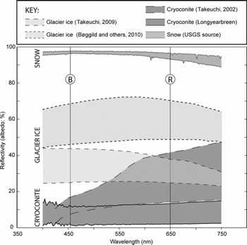
Fig. 2. Apparent ranges of spectral reflectivity of several supraglacial surfaces. The cryoconite data are drawn from Aj. Hodson and R.G. Bryant (unpublished) and (for dry cryoconite) from Reference TakeuchiTakeuchi (2002), the snow reflectance sourced from the US Geological Survey (USGS), while the two sets of data for Arctic glacier ice are taken from Alaska (Reference TakeuchiTakeuchi, 2009) and northeastern Greenland (Reference Bøggild, Brandt, Brown and WarrenBøggild and others, 2010). The latter two studies present spectral response of glacier ice with a range of impurity coverage, so ‘cleaner’ glacier ice reflectance is likely to lie in the upper regions of the range of spectral responses, for which reflectivity in the red channel (centred at R) decreases rapidly in contrast to the increasing response for cryoconite at similar wavelengths. The spectral response of dry cryoconite is likely to be reduced further when the material becomes wet. Note the theoretical basis for differentiating ice and cryoconite in the blue channel (centred on B) where contrast between reflectance is greatest.
Method development
For both laboratory and field applications we employed four discrete steps: (1) calibration of spatial scale (image resolution, mm pixel−1) and associated uncertainties; (2) manual identification and measurement of cryoconite dimensions for use as control datasets; (3) ‘supervised’, semi-automated measurement of cryoconite using standard image-processing functions in ImageJ; and (4) rapid, automated processing of multiple images using custom scripts to identify and measure cryoconite. These steps are schematically illustrated in Figure 1. Each step establishes a set of reference data against which the output of successive steps is compared.
Isolation of cryoconite using image thresholding
Digital image thresholding involves constraining analysis to a subset of the image data for which pixel brightness values fall within a specified range. Since after image preprocessing cryoconite appears darker than other image elements, we assumed that cryoconite granules (laboratory data) or regions on the ice surface (field data) could be isolated by thresholding for those pixels with brightness values which fall below a specified threshold level. This level was specified by a supervised classification in which the threshold was iteratively adjusted until the isolated image pixels best coincide with the locations and limits of cryoconite within the field of view (illustrated in Fig. 1).
Error analysis
Total uncertainty in measurements on vertically oriented (plan-view) images was determined by combining the two key uncertainties derived from (1) calibration of spatial resolution, and (2) operator error in selection of threshold values. We report procedures to estimate both these uncertainties in each protocol. In field data, these methodological uncertainties are compounded by variations arising from changing camera position, surface aspect, ambient lighting and so on. Additional uncertainty arises when reducing spatially distributed data to singular values (e.g. a value for cryoconite coverage averaged over the set of images at any grid-surveyed site). Explicit consideration of all these errors is a non-trivial exercise. Therefore, where applicable, we report uncertainty in field data as simply the standard error (E) on cryoconite area at each survey site, using the standard deviation derived from threshold selection in measurements of cryoconite area from control images (σ) and a t value (p = 0.05) dependent on the control image sample size (n):
Analyses and Results
Cryoconite granule morphometry
Calibration and spatial resolution
The total sample size was 18 digital images, each showing one Petri dish containing five discrete cryoconite granules. The ImageJ LINE tool was used to assess variations in spatial scale by measuring the length (in image pixels) of the 2 mm grid squares in both x and y directions at random locations within each image. There was minimal radial distortion within the images, with a root-mean-square error (RMSE) of 0.06 mm when comparing x- and y-grid dimensions across the area of interest, and a maximum uncertainty of 0.2 mm. Variations in camera height between images were also small and yielded a mean image resolution of 0.09 ± 0.01 mm pixel−1, equivalent to an 11% uncertainty in length measurements.
Manual measurement of granule size
The longest distance across individual granules (A-axis lengths) was measured manually as in previous work (e.g. Reference Takeuchi, Kohshima and SekoTakeuchi and others, 2001). The A-axis for each particle was determined visually and measurements (LINE tool) were repeated three times to provide an estimate of mean user error (±1.3%). The resulting mean granule size for the 90 particles isolated in this analysis was 8.59 ± 6.67 mm. Population mean granule dimensions were reported previously by Reference TakeuchiTakeuchi (2002) and Reference Takeuchi and LiTakeuchi and Li (2008) for elsewhere in the Arctic (0.50 ± 0.29 mm), the Himalaya (0.54 ± 0.21 mm), Tibet (0.80 ± 0.35 mm) and China (1.4 ± 0.47 mm). However, we emphasize that the granules isolated for this study were selected for the purpose of developing the image-processing methodology rather than to be statistically representative of the sampled population. Importantly, the pixel resolution reported above readily permits measurements in these size ranges using the methods presented here (see below).
Semi-automated measurement of granule dimensions
A random selection of five images (25 granules) was analysed using digital image thresholding to isolate cryoconite granules within each image. The threshold level was selected to ensure that the perimeters of the isolated pixel regions coincided exactly with the observed cryoconite granule perimeters. Once this was achieved, the image was converted to a binary (two-colour) image where thresholded regions (cryoconite) were set to black and all other parts of the image set to white (Fig. 1). An OPEN filter was applied to reduce the roughness of the binary ‘particle’ edges. The ANALYZE PARTICLES tool in ImageJ runs an algorithm which scans a binary image to locate and measure discrete pixel areas (‘particles’) which meet specified criteria (e.g. limits on granule area and circularity). It then calculates and returns the dimensions of an ellipsoid best-fitting each particle thus identified (Fig. 1). The tool was applied to the threshold binary images to obtain the Feret diameter (FD), granule area (A) and A-axes of ellipsoids fitted to the cryoconite granules. The minimum particle length dimension measurable by this automated process was 0.27 mm, equal to a granule with plan-view area of 0.07 mm2.
Figure 3a shows that FD measurements obtained using the semi-automated ANALYZE PARTICLES approach were not significantly different (p<0.01) from the manually identified A-axis length, for granules <30 mm in diameter. The same result was achieved for semi-automated measurement of the ellipse A-axes (data not shown). For larger particles the tendency of the semi-automated method to overestimate granule dimensions relative to the manual dataset led to significant discrepancy between the two approaches, although we note that typical cryoconite population bias is towards the smaller (<15 mm) granules for which this issue does not apply. Image processing was replicated independently and yielded an average variance in choice of threshold level of approximately eight digital brightness units (DN). Repeating the image processing using a range of ±5 DN about the mean threshold value enabled the maximum relative error of thresholding to be estimated as 16.6 ± 6.02% and 10.0 ± 3.51% for granule area and FD values, respectively. Probabilistically combining these values with the uncertainties in image resolution, noted previously, yielded total errors in granule area and FD measurements of <20%.
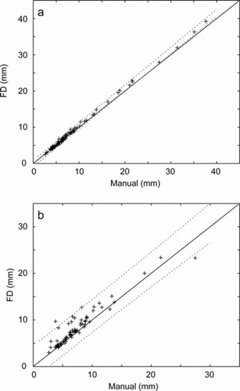
Fig. 3. Plots of (a) semi-automated measurement of cryoconite granule FD against manually measured granule long axis; and (b) manual measurements against the fully automated batch-processed retrieval of FD using ImageJ’s internal auto-threshold. The dashed lines indicate confidence limits for the TLS regression (p = 0.01) and the solid line indicates the 1:1 relationship.
Fully automated (batch) measurement of granule dimensions
We developed a simple automation algorithm (macro) coded in the ImageJ scripting language. The objective was to enable rapid, standardized quantification of cryoconite granules in a set of images obtained under identical conditions. The macro (Appendix A) collates a set of raw images as a STACK, performs the pre-processing outlined earlier and sets ImageJ measurements to include FD, area and the A-axis of ellipses fitted to cryoconite granules. The user is given the option of using automated thresholding in individual images or entering a single supervised threshold value applicable to the entire dataset. The macro then performs on each image in turn the THRESHOLD, CONVERT TO BINARY and ANALYZE PARTICLES routines described above.
Unsupervised (auto-thresholding) batch processing of the entire image set using the macro yielded an 86% success in identifying granules. Figure 3b shows that there was no significant difference from a 1:1 relationship (p = 0.01) between measurements of granule FD by fully automated and manual techniques, despite respective methodological uncertainties of ±10.1% and 1.3%. Supervised processing (requiring a user-defined threshold) increased the success of granule identification to 91%. Failure to identify granules, or instances of substantial deviation between automated and manual measurements for individual granules, was attributed to the presence of shadows, particularly around larger granules, reflecting non-ideal lighting conditions and demonstrating how the method may be readily improved.
Critically, supervised or automated thresholding is operator- or image-dependent and therefore represents a major potential source of error in reported measurements. To illustrate the sensitivity of the measurements to threshold selection, we performed the batch processing with the choice of supervised threshold spanning ten brightness levels (i.e. ±5 DN about the specified ‘optimum’). Figure 4a shows the effect of variation in threshold on the mean and standard deviation of FD measurements. It is obvious that in laboratory data the variation in threshold makes little impact on the measurement of cryoconite granule geometry, in particular in comparison to the size variation in the sample as a whole (characterized by standard deviation error bars). This is a function of the high brightness contrast between dark cryoconite and bright background image pixels (Fig. 4a).
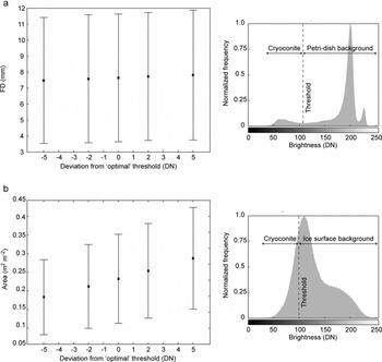
Fig. 4. Graphs illustrating the influence of uncertainty in threshold value (DN) on (a) the mean geometry (FD) for a sample of 84 granules, and (b) the mean cryoconite area taken from a 16-image survey. Error bars are given as the standard deviation of all measurements. Sample histograms for the two image types are given for comparison.
Correlation between granule dimensions and morphology
We observed that the granules appeared more elliptical in shape as their dimensions increased. To quantify this we measured the circularity of the granules. ImageJ includes an algorithm for circularity, C, determined as:
for which P is the granule perimeter. A plot of granule circularity against A-axis (Fig. 5) showed a clear trend for larger granules to be less circular (and, by inference, less spherical). We emphasize that our analyses are limited to the two-dimensional (2-D) shape of the circumference of the upper surface of each granule presented to the camera lens. However, these observations imply that the processes of cryoconite granule growth may not be uniform across the granule surface; this indicates an area for future research. Cryoconite granules grow through the activity of bacteria and algae on the granule surface (Reference Takeuchi, Kohshima and SekoTakeuchi and others, 2001; Reference HodsonHodson and others, 2010), and the non-spherical form may therefore reflect a biologically mediated balance between growth (and erosion) kinetics and heterogeneous, physical aggregation properties.
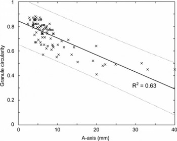
Fig. 5. Plot of elliptical A-axis against actual granule (plan-view) circularity illustrating a significant negative relationship between the variables. The dashed lines indicate confidence limits for the TLS regression (p = 0.01), and the solid line indicates the 1:1 relationship.
Spatial variability in supraglacial cryoconite extent
Calibration and spatial resolution
From each of the seven GrIS survey sites, images were selected at random (up to six images per site) for use as control data. In each image, the scale on the quadrat placed on the ice surface was manually measured four times in the vertical and horizontal. The average RMSE when comparing a total of eight x and y dimensions across the area of interest was <0.32 mm, indicating little distortion over a region of interest (ROI) ∼40 × 40 cm centred on the image centre. Mean pixel resolution across all images was 0.03 ± 0.002 cm pixel−1, with a range of 0.021–0.039 cm pixel−1 across the seven survey locations.
Manual measurement of cryoconite area
Control images were manually thresholded as described previously to carefully define regions of cryoconite, and this supervised threshold value recorded for each individual image. The ImageJ MEASURE tool was used to quantify the area occupied by cryoconite (m2 cryoconite m−2 surface) within the field of view (steps illustrated in Fig. 1). Independent replication of threshold selection yielded a range of ±5 DN. This range was used to estimate the uncertainty due to threshold selection on measurements of cryoconite area in each control image. The mean uncertainty over all control images was used as a measure of the likely errors within the survey as a whole. This assessment gave an overall mean uncertainty of ±22.7% on measurements of cryoconite area, with values ranging from ±10% to ±48%within each of the seven survey sets. Combination of these errors with the resolution uncertainty yielded a mean methodological error of 23.3% in cryoconite area estimates across the control image set.
Semi-automation of image analysis
All images from each survey were processed using an ImageJ macro (Appendix B) to automate the analysis. Due to the variations in exact quadrat position in each image, measurements of cryoconite coverage were limited to an ROI measuring 25 × 25 cm centred on the centre of the image. The mean supervised threshold value obtained from the manual analysis of control images at each survey site was applied to all images at that site, and the area identified as cryoconite in each image was obtained using the MEASURE tool. Fully automated processing (i.e. unsupervised threshold selection to isolate pixels corresponding to cryoconite in each image) was not possible in these data due to the lower contrast between ice surface types in field data, as discussed in the methods section.
To demonstrate the sensitivity of threshold selection on cryoconite area estimates, we performed the processing routine with supraglacial images for a single survey and employed a threshold range ±5 DN about the mean ‘optimum’ derived from the corresponding control images. Over the 16 field images, the 10 DN variation in threshold led to a 50% increase in the average area identified as cryoconite, with a similar trend in the variation of sample image measurements as a whole (Fig. 4b). The sample histogram, combined with inspection of Figure 1, shows that there is typically much lower brightness contrast between cryoconite regions and other ice surface types in these images. Thus, in field data, careful supervision of the image threshold selection is critical to the accuracy of measurements, and an allowance for operator error during this supervision may contribute to a substantial uncertainty in measurements of supraglacial cryoconite area.
Results for the GrIS transect are presented in Figure 6, which shows the variation in mean supraglacial cryoconite extent for each survey site against distance from the ice margin. Uncertainty in a singular, representative cryoconite area for each survey was estimated using the standard error (E in Equation (1)) derived from the control images, which yielded a mean uncertainty of 0.154 m2 cryoconite m−2 surface, or ∼37% across all seven survey sites. The results presented in Figure 6 indicate reductions in cryoconite extent above ∼550 m a.s.l. and below ∼510 m a.s.l. The actual elevational loading of cryoconite material could be readily estimated from our data by using calibration images containing a known mass of cryoconite (refer to Reference HodsonHodson and others (2007) for method) but is not explored further here. However, if the strong linear relationship between debris mass and apparent surface area coverage found by Reference HodsonHodson and others (2007) for midtre Lovénbreen, Svalbard, is applicable to GrIS, the results here indicate highly varied debris concentrations over elevation in the ablation area at the study site.
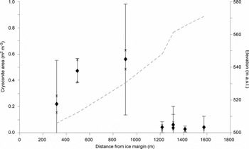
Fig. 6. Plot of cryoconite extent (m2 m−2) against distance from ice margin across an up-glacier transect in the ablation zone on GrIS. Elevation for the same transect is indicated by the dashed line. Cryoconite extent is given as the mean determined by batch processing of all images collected on a grid-based survey at each site, and uncertainty bars are given as the standard error (E) derived from the subset of control images for each survey estimating spatial uncertainties. Methodological uncertainty limits are indicated with ‘x’.
Placed in context, our results appear to corroborate earlier observations by Reference Oerlemans and VugtsOerlemans and Vugts (1993) who were the first to highlight a darker zone in the upper ablation area of GrIS. Similarly, more recently Reference Bøggild, Brandt, Brown and WarrenBøggild and others (2010) report a lowered albedo in the upper ablation zone away from the ice margin at another site on GrIS in response to cryoconite volume and dispersal. The glaciological application of the method presented allows rapid quantification of imagery, in combination with meteorological, radiation or reflectance measurements, to explore empirical relationships and test assumptions regarding the characteristics of ice surface materials and processes: for example, whether dust and debris (cryoconite) is greatest at the lowest elevations in the ablation zone (e.g. Reference OerlemansOerlemans, 1992; Reference Brock, Willis and SharpBrock and others, 2000); or whether cryoconite or meltwater present primary controls on supraglacial albedo (cf. Reference BøggildBøggild, 1998; Reference GreuellGreuell, 2000).
Temporal variability in supraglacial cryoconite extent
Calibration and spatial resolution
As the distance between the fixed camera and the ice surface increased due to ablation, the spatial resolution of images changed over the time series. To quantify this variation, the apparent maximum diameter of a 47 mm white filter paper, placed on the ice surface, was measured in each image to obtain the pixel resolution (mm pixel−1). Since the pixel resolution changed significantly and systematically within the dataset (0.13–0.17 mm pixel−1), the size of the ROI corresponding to an area of 20 × 20 cm varied from image to image. However, using the known image resolution, the dimensions (in pixels) of a scale-consistent ROI centred on the source image centre point could be readily calculated and defined using the ImageJ MAKE RECTANGLE script.
Manual measurement of cryoconite area
Calibrated images at 6 hour time intervals were manually thresholded to isolate regions of cryoconite as described earlier. This supervised threshold value was recorded for each individual image. The MEASURE tool was used to quantify the area occupied by cryoconite. Note that this procedure therefore measures the pixel area in the image occupied by material identified colorimetrically as cryoconite; it is not a measure of the area of the holes in which cryoconite particles may reside. Uncertainty in the area retrieved for each ROI was estimated using the ±5 DN variance in the threshold level assumed from the previous analyses, and validated, again independently, by replicate analyses: for each image, uncertainty was given as 2σ in area measurements over the range of threshold values. The mean uncertainty in cryoconite area across the 41 images in the time series was estimated to be ±22%.
Automated measurement of cryoconite area
The custom macro (Appendix B) was extended to perform supervised and fully automated measurement of cryoconite area. Supervised measurements require the user to input the mean cryoconite threshold level based on manual analysis for a given set of images; automated measurements use the AUTO-THRESHOLD function in ImageJ.
Figure 7 illustrates the results of the time-series analysis at 6 hour time intervals. There was typically a relatively small difference between amounts of cryoconite measured using manual, supervised or automated techniques, within the limits of error established for the imaging in general. However, instances occurred where the fully automated approach showed substantial deviations from the manual results. Post hoc examination showed these deviations tended to coincide with significant changes in imaging conditions (colour levels, lighting and shadowing) as had been seen with the GrIS images. Nonetheless, removal of these outlying data should be a simple process using a series of manually processed control images. Over the 9 day duration of observations at the Longyearbreen site, the data demonstrate an apparent trend of decreasing extent of cryoconite (r2 = 0.23, slope of the regression significant at p = 0.05). The apparent variability at shorter time-steps indicates some form of temporal dynamics: these may (1) relate to variations in lighting and shadowing as solar position changes with respect to the ROI or (2) reflect differing melt processes as relative fluxes of incident and turbulent energy co-vary with changing meteorological conditions resulting in the melt-in and melt-out of cryoconite debris (Reference HodsonHodson and others, 2008, Reference Hodson2010). However, further analysis is required before causal mechanisms or feedbacks can be identified.
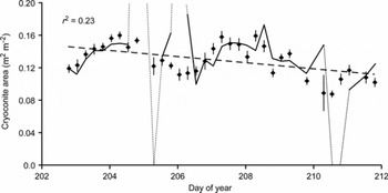
Fig. 7. Chart illustrating the temporal change in supraglacial cryoconite extent (m2 m−2) on Longyearbreen during 2007 as indicated by points. Error bars, for area determined for each image, were estimated from analysis of the variance of area in response to the ±5 DN range of uncertainty in threshold value. The trend in extent over time is shown as a dashed line based on a linear regression and includes the r 2. The solid line shows the results for fully automated batch processing of the same suite of images, illustrating close agreement in some areas and marked divergence (dotted line) in others suggestive of the issues relating to environmental conditions (especially lighting).
Acquisition of time-lapse imagery of the ice surface, as demonstrated here, could be used to test the notions of cryoconite mobility within the supraglacial environment suggested by Reference HodsonHodson and others (2010). With respect to the larger-scale glaciological impacts, variability in cryoconite coverage clearly has implications for albedo (e.g. Reference Bøggild, Brandt, Brown and WarrenBøggild and others, 2010), and short-term spatial and temporal variability in albedo has been widely documented (e.g. Reference BrockBrock, 2004). Sub-centimetre scale image data afford the opportunity to explore redistribution of supraglacial debris by ‘surface washing’ during heightened melt or precipitation events (Reference BrockBrock, 2004) and to examine the complex interplay between cryoconite coverage, meteorology and surface albedo at a variety of timescales.
Conclusions
In summary, we demonstrate a novel measurement methodology, and report associated errors, which enables rapid, semi-automated batch processing of digital images to obtain cryoconite granule geometry and in situ supraglacial areal extent in Arctic settings. The methods provide standardized tools for handling the large quantities of data sourced from field studies that sample the ice surface at high spatial and temporal resolution and at a large number of survey sites. The method is shown to be feasible for surface cryoconite as found in Arctic (and more temperate) environments, but its use in Antarctic settings where ice lids typically cover cryoconite aggregations remains to be explored. Useful data can be obtained using inexpensive, lightweight digital cameras, making intensive studies more viable. Such an approach enables quantitative exploration of both the spatial and temporal variations in cryoconite coverage and form which can be readily linked to the potential impacts on ice-sheet surface mass balance or the physical and biogeochemical dynamics of this important ecological niche. In supporting this, these methods facilitate the key step change from research at few sites on the valley-glacier scale to research spanning many sites across the ice-sheet scale (Reference HodsonHodson and others, 2008).
We have identified several key factors determining the quality of the data analysis: ambient lighting and its variability between images is critical. In the laboratory, this particularly affected larger granules; their shadows made accurate identification of granule edges by a brightness threshold challenging. Improved results could be achieved by using a light table such that the granules are lit from both above and below, thereby eliminating shadows. The use of portable USB microscopes (e.g. Veho VMS-004 Discovery) capable of directly capturing images means that our methodology could be applied in temporary field laboratories and for granules considerably smaller than those reported here. Variability of environmental conditions in the field dictates that ambient light cannot be readily controlled or constrained. Nonetheless, the methodologies presented here allow rapid extraction of information pertaining to the dynamics of supraglacial cryoconite distribution with remarkably little data loss. The quantitative image analyses presented here facilitate the acquisition of primary data to support studies of cryoconite granule growth mechanisms and constraints; supraglacial debris formation, mobility and evolution; and assessment of ice surface albedo variations linked to the dynamics of cryoconite coverage.
Acknowledgements
A.J.H. acknowledges The Leverhulme Trust (Research Fellowship No. RF/4/RFG/2007/0398), and J. Yde, D. Pearce and K. Cameron for their help during fieldwork. T.I.F. acknowledges UK Natural Environment Research Council (NERC) standard grant NE/G006253/1. J.W.B. was supported in this work by S. Banwart and the NERC (grant NE/C521001/1). Helpful and thoughtful reviews by N. Takeuchi and E. Bagshaw aided improvement of the manuscript, and the Scientific Editor, J. Glen, is also thanked.
Appendix A

Appendix B


