


Nomenclature
- GNC
-
guidance, navigation and control
- NSY
-
non-symmetrical shape
- SY
-
symmetrical shape
- HY
-
hybrid shape
- PID
-
proportional, integral, derivative
- LQR
-
linear quadratic regulator
- ${P^*}$
,
$P_{nd}^*$
${P^*}$
,
$P_{nd}^*$
-
Pareto front; non-dominated solution sets
- Sp
-
simulation platform
-
$G(t)$
,
$P(t)$
-
initial populations – store files
-
${J_i}({S{P_{{\theta _g}}}})$
-
objective function
- Ixx, Iyy, Izz
-
moment of inertia about X, Y, and Z axes
- I
-
MASS distribution dataset
- SV
-
search volume
-
$nbo{x_i}$
-
trajectory container box
- B
-
the set used to assign or distribute the trajectories
-
$J({S{P_{{\theta _g} - \epsilon}}})$
-
objective function with elitist concept
-
${G_{CAD}}$
-
computer-aided design – CAD model physical attributes
-
${T_{thrust}}$
-
thrust model motion simulation
-
${H_s}$
-
identified thrust model
-
${Z_{guess}}$
-
initial values for trim point optimisation
-
${J_i}$
-
performance indices impacted by geometry optimisation
-
${f_{ij}}$
-
multiple objectives for decision-making
-
${u_j}$
-
the reference utopian point
-
$V$
-
electric potential in voltage ((volts))
-
$C$
-
discharge capacity of the battery ((mAh))


Greek symbol
-
$\epsilon $
-
elitist concept
-
${\theta _g}$
-
target geometric variable
-
${\lambda _a}$
-
length from centre of mass to nose motor
-
${\lambda _b}$
-
length from centre of mass to tail motor
-
$\alpha $
-
angle between the nose arms
-
$\beta $
-
angle between the tail arms


1.0 Introduction
Unmanned aerial vehicles (UAVs), particularly multirotors, are central in research on autonomous guidance, flight control and dynamic modelling. Moreover, racing drones offer a demanding testbed for studying how airframe geometry shapes real-world performance. Along these lines, this study introduces a modelling and optimisation framework grounded in previously validated experimental benchmarks that unifies geometric design, control and a co-simulation platform, coupling an elitist multi-objective evolutionary search with implicit numerical routines and integration to propagate geometry changes into trajectory-level flight dynamics in a consistent and reproducible way.
1.1 Literature review
Over the past 15 years, advances in miniaturisation and the enhanced capabilities of on-board companion computers have undeniably propelled autonomous control techniques [Reference Hanover, Loquercio, Bauersfeld, Romero, Penicka, Song, Cioffi, Kaufmann and Scaramuzza1]. However, this progress also highlights the need to reconsider the airframe as a fundamental flight enabler that integrates dynamic responses often misrepresented by the limitations of on-board sensors [Reference Rojas-Perez and Martínez-Carranza2, Reference Yu, Tang, Song and Lin3]. At the core of this challenge lies a critical issue: how to interpret flight behaviour shaped by non-traditional dynamics.
Most conventional approaches to this sort of dynamic problem identify wings or actuators as the primary flight enablers. Within the approaches, the methods applied typically model the system as a rigid multibody structure connected through rotational joints [Reference Bergonti, Nava, Wüest, Paolino, L’Erario, Pucci and Floreano4–Reference Mintchev and Floreano7]. Thus, the corresponding mathematical frameworks focus on the range of positions that wings or arms can adopt, determined by the degrees of freedom allowed by these joints. In such models, trajectory analysis relies on changes in the location of these components, with the goal of optimising the control gains enclosed by a path planning problem. Although these methods are the most widespread, the approaches that contain them do not evaluate how variations in the structural shape of the flight enabler affect overall flight performance. As a result, they overlook the role of geometric shaping in enhancing specific flight indices.
Alternatively, these methods, in practice, aim to adjust the angular separation between drone arms or wing placement and adapt control gains to optimise energy efficiency based on the characterised trajectory during the mission [Reference Kim, Lee, Jeong and Myung8–Reference Falanga, Kleber, Mintchev, Floreano and Scaramuzza10]. Since these alternatives are typically validated in real-time conditions, the desired flight behaviour tends to prioritise steady-state flight constraints to guarantee a safe flight test. Despite these tests providing valuable flight performance information, flight behaviour is not readily generalisable, as performance is often assessed under mission- and platform-specific experimental conditions and reporting practices [Reference Asignacion and Suzuki11, Reference Grøntved, Jarabo-Peñas, Reid, Rolland, Watson, Richards, Bullock and Christensen12]. Besides that, the flight tests also lack a broadly adopted standardised metric set that allows establishing a comparable range or limit for the modelled flight behaviour across platforms (i.e., a baseline dynamic response for cross-model comparison) [Reference Campbell, Gregory, Acheson, Ilangovan and Ranganathan13–Reference Cwiakala15]. As a result, they have a narrow view and disregard the integrated contribution of all structural and principal flight enablers. Fundamentally, these initiatives focus on evaluating specific aspects of flight dynamics independently, often enhancing the body structure with non-essential flight enablers. While they contribute to subsystem-level understanding, they generally prioritise local performance indicators over a holistic assessment of dynamic behaviour and overall system performance.
A small number of less conservative and more recent initiatives have attempted to overcome the geometric constraints of conventional quadrotors by proposing alternative body airframe configurations, often prototypes of bespoke geometric shapes or with more than six arms [Reference Li16, Reference Pollet, Delbecq, Budinger and Moschetta17]. These unconventional designs highlight the relevance of non-traditional dynamic modelling and provide valuable contributions to the literature. While they present intuitive conceptual approaches and mathematically sound formulations, their applicability to practical implementation scenarios remains limited in scope and detail. In particular, from a control and optimisation perspective, these approaches emphasise trajectory generation and system response but tend to leave the relationship between control effort, voltage demand and energy consumption unspecified. As a result, the system’s ability to reliably track a trajectory under varying conditions remains insufficiently characterised. As new airframe designs continue to enrich the conceptual landscape, it is also a common practice for them to rely on conjectural or unsystematic frameworks with limited and inconclusive empirical grounding. Hence, this reinforces the need for rigorous experimental validation to confirm and generalise any claimed improvements in flight efficiency associated with this essential flight enabler.
Under this overarching theme, complementary studies embrace the experimental approaches and simulation techniques within systematic validation frameworks [Reference Castiblanco, Garcia-Nieto, Simarro and Ignatyev18, Reference Castiblanco, Garcia-Nieto, Simarro and Salcedo19]. The experimental studies emphasise the geometric structure of the body and employ descriptive statistics within robust methodologies to characterise and model the non-traditional dynamics observed in racing-quality drones [Reference Castiblanco, Garcia-Nieto, Simarro and Salcedo20] and conventional categories [Reference Teng, Yu, Luo, Wang and Zhang21, Reference Sóbester, Keane, Scanlan and Bressloff22]. In a nutshell, they have organised case studies and examined how different geometric configurations of quadrotor bodies relate to the dynamic behaviour observed during the recorded flight trajectories. Furthermore, the pilots’ technical expertise is integrated into the loop and combined with large volumes of sensor data, strengthening mathematical modelling. While this approach yields accurate and reliable flight information under complex navigation scenarios, it remains limited by the absence of a suitable reference threshold for dynamic performance. By configuring the experimental conditions so that the airframe functions as a unifying flight enabler, it becomes possible to compare sorts of performance indices within an appropriate optimisation procedure. In this context, the measurable ranges would be defined by the trajectories flown and the flight behaviour of both standard and optimised bodies, providing a yardstick for performance assessment. This methodological approach could enable a structured evaluation of the airframe’s role as a dynamic unifier, bridging empirical validation with optimisation via mathematical modelling.
1.1.1 Significant prior foundations
This study builds upon previous scientific reviews to consolidate a line of prior research outputs [Reference Castiblanco, Garcia-Nieto, Simarro and Ignatyev18–Reference Castiblanco, Garcia-Nieto, Simarro and Salcedo20, Reference Castiblanco, Garcia-Nieto, Ignatyev and Blasco23]. The means of doing so is to integrate its key developments into a unified framework for investigating drone flight dynamics and evaluating performance within a global multi-objective optimisation scheme. Among the key aspects, the generalisation of geometric shapes stands out, which experimentally captures how the configurations of the body’s airframe influence the dynamics of drones.
Figure 1 synthesises geometric shape patterns using three key parameters: ( $\alpha $
) alpha, (
$\alpha $
) alpha, ( $\beta $
) beta and (
$\beta $
) beta and ( ${\lambda _a},{\lambda _b}$
) lambda. The angles
${\lambda _a},{\lambda _b}$
) lambda. The angles $\alpha $
and
$\alpha $
and $\beta $
define the arm configuration space, while
$\beta $
define the arm configuration space, while ${\lambda _a}$
and
${\lambda _a}$
and ${\lambda _b}$
denote the semi-diagonal distances measured from the centre of mass to the motors along each of the two opposing diagonals. This split parameterisation is intentionally adopted to provide finer geometric control during modelling and simulation, whilst the corresponding motor-to-motor diagonal can be recovered as
${\lambda _b}$
denote the semi-diagonal distances measured from the centre of mass to the motors along each of the two opposing diagonals. This split parameterisation is intentionally adopted to provide finer geometric control during modelling and simulation, whilst the corresponding motor-to-motor diagonal can be recovered as $\lambda = {\lambda _a} + {\lambda _b}$
(with
$\lambda = {\lambda _a} + {\lambda _b}$
(with ${\lambda _a} = {\lambda _b} = \lambda /2$
in the symmetric case). The generalisations govern, constrain and shape the range space of feasible body geometries, and based on these parameters, three generalised cases of airframes are defined. The nominal case corresponds to symmetric geometries, where
${\lambda _a} = {\lambda _b} = \lambda /2$
in the symmetric case). The generalisations govern, constrain and shape the range space of feasible body geometries, and based on these parameters, three generalised cases of airframes are defined. The nominal case corresponds to symmetric geometries, where $\alpha = \beta = {90^ \circ }$
. The fixed asymmetric case includes non-symmetric geometries in which
$\alpha = \beta = {90^ \circ }$
. The fixed asymmetric case includes non-symmetric geometries in which $\alpha $
and
$\alpha $
and $\beta $
deviate by the same angular magnitude, preserving structural equilibrium. The variable asymmetric case encompasses configurations where only one of the angles varies, thus generating a hybrid family of airframes. In all cases, the semi-diagonal parameters (
$\beta $
deviate by the same angular magnitude, preserving structural equilibrium. The variable asymmetric case encompasses configurations where only one of the angles varies, thus generating a hybrid family of airframes. In all cases, the semi-diagonal parameters ( ${\lambda _a},{\lambda _b}$
) remain variable, enabling a broad and systematic exploration of geometry-induced dynamic effects.
${\lambda _a},{\lambda _b}$
) remain variable, enabling a broad and systematic exploration of geometry-induced dynamic effects.
Geometric generalisation used for drone airframe optimisation [Reference Castiblanco, Garcia-Nieto, Simarro and Salcedo19]. The nose (forward) direction is defined by the body-fixed $ + y$
axis.
$ + y$
axis.

The development of an earlier platform for simulating trajectories is outlined in Fig. 2. It represents another key aspect of this work and marked the first attempt to mathematically model the dynamic problem using prior information derived from experimental flight tests.
Overall outline of the platform for trajectory simulation [Reference Castiblanco, Garcia-Nieto, Simarro and Salcedo20].

Figure 3 illustrates two behavioural indices related to acceleration across curved and straight sectors. Building on previous findings, acceleration changes observed in curved sectors are not driven by variations in speed but rather by directional changes and the interaction with different arm angle configurations. The robustness of the analysis is supported by statistical inference drawn from over one million data points analysed per model tested, with all datasets stored in the TRAM-FPV database [Reference Castiblanco, Garcia-Nieto, Ignatyev and Blasco23]. A detailed description of the complete methodology and statistical validations can be found in Ref. [Reference Castiblanco, Garcia-Nieto, Simarro and Ignatyev18]. Accordingly, the modelling of the initial platform enables the integration of the evolutionary algorithm, while the previous experimental results will be contrasted with those obtained through the coupled computational modelling to establish dynamic performance ranges. In plain words, trajectories derived from optimised body–airframe geometries are compared against those of baseline configurations to establish a benchmark through selected performance indices. The approach adopts a holistic–heuristic modelling strategy that brings together geometric design, motion dynamics and control algorithms within a single simulation platform. This integration minimises bias from non-essential flight enablers and enables system-level analysis of how structural variation influences flight behaviour [Reference Akter, McCarthy, Sajib, Michael, Dwivedi, D’Ambra and Ning Shen24, Reference França and Garcia-Patron25].
Prior flight performance results [Reference Castiblanco, Garcia-Nieto, Simarro and Ignatyev18].

In summary, two general nominal cases are established in prior research [Reference Castiblanco, Garcia-Nieto, Simarro and Ignatyev18, Reference Castiblanco, Garcia-Nieto, Simarro and Salcedo19]: the symmetric and the asymmetric layouts. The symmetric case corresponds to the family of models denoted as SY, where both arm angles are equal to ${90^ \circ }$
. In contrast, the asymmetric case comprises two subfamilies: the hybrid structures (HS), in which one arm angle remains fixed at
${90^ \circ }$
. In contrast, the asymmetric case comprises two subfamilies: the hybrid structures (HS), in which one arm angle remains fixed at ${90^ \circ }$
while the other varies, and the non-symmetric structures (NSY), where both arm angles deviate equally from
${90^ \circ }$
while the other varies, and the non-symmetric structures (NSY), where both arm angles deviate equally from ${90^ \circ }$
. These abbreviations (SY, HS and NSY) are commonly adopted in the literature and will be consistently used throughout this manuscript.
${90^ \circ }$
. These abbreviations (SY, HS and NSY) are commonly adopted in the literature and will be consistently used throughout this manuscript.
1.1.2 Chain of reasoning
Airframe geometry is encoded as decision variables $\theta $
and evaluated in a multiparadigm co-simulation that links CAx thrust and physical properties with the control architecture. The chain builds on a validated co-simulation platform and experimentally validated benchmarks [Reference Castiblanco, Garcia-Nieto, Simarro and Ignatyev18–Reference Castiblanco, Garcia-Nieto, Simarro and Salcedo20]. A trimming step and the linear state model define the plant used to propagate trajectories, and performance indices
$\theta $
and evaluated in a multiparadigm co-simulation that links CAx thrust and physical properties with the control architecture. The chain builds on a validated co-simulation platform and experimentally validated benchmarks [Reference Castiblanco, Garcia-Nieto, Simarro and Ignatyev18–Reference Castiblanco, Garcia-Nieto, Simarro and Salcedo20]. A trimming step and the linear state model define the plant used to propagate trajectories, and performance indices $J(\theta)$
(speed, acceleration, lap time, controller effort, pitch) quantify behaviour under identical controller settings and battery voltage constraints. The search is conducted in a high-dimensional objective space where Pareto sets are approximated by a hybrid strategy that combines finite differences and Nelder–Mead with an elitist evMOGA. Candidate trajectories are benchmarked against validated references to assess efficiency and feasibility. This chain (geometry
$J(\theta)$
(speed, acceleration, lap time, controller effort, pitch) quantify behaviour under identical controller settings and battery voltage constraints. The search is conducted in a high-dimensional objective space where Pareto sets are approximated by a hybrid strategy that combines finite differences and Nelder–Mead with an elitist evMOGA. Candidate trajectories are benchmarked against validated references to assess efficiency and feasibility. This chain (geometry $ \to $
simulation
$ \to $
simulation $ \to $
control
$ \to $
control $ \to $
indices
$ \to $
indices $ \to $
optimisation
$ \to $
optimisation $ \to $
benchmarking) ensures that observed gains and transients are attributable to geometry rather than gain retuning and provides a consistent basis for selecting high-agility designs.
$ \to $
benchmarking) ensures that observed gains and transients are attributable to geometry rather than gain retuning and provides a consistent basis for selecting high-agility designs.
1.2 Paper structure
Section 1 motivates the study, identifies a gap around geometry-driven flight dynamics and sets prior experimental and simulation foundations. It generalises the airframe using $( {\alpha ,\beta ,\lambda })$
, anchors the work in a validated trajectory and simulation platform and frames the nominal families SY, HS and NSY as baselines. Section 2 formalises the optimisation problem and the numerical backbone (finite differences, Nelder–Mead, elitist evMOGA-epsilon dominance) within a co-simulation workflow that links CAx thrust modelling with MATLAB/Simulink control logic via an S Function. Section 3 states the working hypothesis and defines the multi-objective vector
$( {\alpha ,\beta ,\lambda })$
, anchors the work in a validated trajectory and simulation platform and frames the nominal families SY, HS and NSY as baselines. Section 2 formalises the optimisation problem and the numerical backbone (finite differences, Nelder–Mead, elitist evMOGA-epsilon dominance) within a co-simulation workflow that links CAx thrust modelling with MATLAB/Simulink control logic via an S Function. Section 3 states the working hypothesis and defines the multi-objective vector $J(\theta)$
over seven geometry-related decision variables and practical bounds, together with the epsilon boxing that structures the search space and maps shape changes to performance indices. Section 4 details how the subroutines are integrated: algorithm execution and the end-to-end flow (thrust modelling
$J(\theta)$
over seven geometry-related decision variables and practical bounds, together with the epsilon boxing that structures the search space and maps shape changes to performance indices. Section 4 details how the subroutines are integrated: algorithm execution and the end-to-end flow (thrust modelling $ \to $
trim
$ \to $
trim $ \to $
linear state space
$ \to $
linear state space $ \to $
linear quadratic regulator (LQR)), including a concise walkthrough from
$ \to $
linear quadratic regulator (LQR)), including a concise walkthrough from ${\theta _g}$
to evaluated indices
${\theta _g}$
to evaluated indices ${J_i}({S{P_{{\theta_g}}}})$
. Section 5 specifies the experimental and algorithmic setup: four waypoints on a
${J_i}({S{P_{{\theta_g}}}})$
. Section 5 specifies the experimental and algorithmic setup: four waypoints on a $50 \times 2.5$
m track, solver limits, identified thrust model, decision criteria; while Section 6 reports Pareto fronts, candidate sets O1 and O2 and comparative metrics used to select representative solutions. Finally, Section 7 summarises the findings and discusses their implications for racing-quality flight dynamics: how the optimised geometry reshapes trajectory-level performance and reduces lap time while keeping thrust and effort (controller stress) within experimentally validated bounds, providing design guidance for high-performance quadrotors.
$50 \times 2.5$
m track, solver limits, identified thrust model, decision criteria; while Section 6 reports Pareto fronts, candidate sets O1 and O2 and comparative metrics used to select representative solutions. Finally, Section 7 summarises the findings and discusses their implications for racing-quality flight dynamics: how the optimised geometry reshapes trajectory-level performance and reduces lap time while keeping thrust and effort (controller stress) within experimentally validated bounds, providing design guidance for high-performance quadrotors.
2.0 Technical description of the optimisation problem
Figure 4 builds upon the co-simulation foundation introduced in previous work [Reference Castiblanco, Garcia-Nieto, Simarro and Salcedo20], where CAx-based environments and trajectory control modules were initially modelled and integrated. The current platform extends this foundation by embedding hybrid numerical routines and decision-making strategies within a unified optimisation framework tailored to flight dynamics and racing drone design.
Hierarchical classification of numerical methods integrated into the simulation platform (problems, solvers and computational approaches).

The diagram in Fig. 4 offers a structured overview of the numerical methods that support this framework, showing how mathematical problems are decomposed, categorised and addressed using both classical and heuristic approaches. It is organised into two hierarchical levels. The top level presents six fundamental categories of numerical problems: optimisation, quadrature, eigenvalue, differential equations and partials, function evaluation and systems of equations. Each category is linked to a sub-level listing the most common analytical methods for its solution. These categories follow widely accepted classifications in numerical analysis [Reference Kiusalaas26–Reference Süli and Mayers28]. The blue boxes in the sub-level show the methods implemented in the platform, such as Gaussian integration for quadrature, singular value decomposition (SVD) for singular value problems and multistep methods for nonlinear systems. For systems of equations, Gaussian elimination and Cholesky decomposition are applied as direct approaches, while Jacobi-stationary method is used for iterative refinement. Other classical techniques, including linearisation via Jacobian matrix, support the numerical solution of the equations of motion (Equations 1–7).
The lower level classifies the computational strategies used to implement these methods. They are grouped into three main branches [Reference Conway29–Reference Dorn31]: Heuristic approaches, iterative schemes and probabilistic algorithmic frameworks. So that, the simulation platform employs three governing methods: finite differences for numerical derivatives, the Nelder–Mead simplex method for unconstrained search and an elitist evolutionary multi-objective genetic algorithm (ev-MOGA), where elitism preserves the best (non-dominated) solutions from one generation to the next to prevent deterioration [Reference Kalyanmoy32, Reference Zitzler, Laumanns and Thiele33]; to compute and display the Pareto front in complex design spaces [Reference Archetti and Grazia Speranza34–Reference Zheng and Liu36], as in Equation (10). Together with the guidance, navigation and control (GNC) subroutines, these methods constitute the algorithmic system. At its core, the control logic activates the GNC subroutines, sets their execution order and defines the conditions under which they run.
 \begin{align}F( {{\bf{n}}[k]}) = F( {{{\bf{n}}_0}}) + E \cdot \left( {\frac{{{\bf{x}}[k] - {\bf{x}}\left[ {k - 1} \right]}}{{{T_s}}} - {{\dot {\bf{x}}}_0}} \right) + A{\rm{'}} \cdot \left( {{\bf{x}}[k] - {{\bf{x}}_0}} \right) + B{\rm{'}} \cdot \left( {{\bf{u}}[k] - {{\bf{u}}_0}} \right) \end{align}
The subroutines of the GNC model employ the numerical method known as the Newton quotient, or difference quotient, to solve Jacobian derivatives that linearise the non-linear functions involved (see the decomposition in Equation 1). The first Jacobian is represented as $E$
, the second as
$E$
, the second as $A{\rm{'}}$
and the third as
$A{\rm{'}}$
and the third as $B{\rm{'}}$
. The matrix
$B{\rm{'}}$
. The matrix $E$
corresponds to the input variable
$E$
corresponds to the input variable $\dot x$
,
$\dot x$
, $A{\rm{'}}$
influences the state variables
$A{\rm{'}}$
influences the state variables $X$
and
$X$
and $B{\rm{'}}$
affects the control actions. The computation is performed implicitly and iteratively until the equations of motion are balanced according to the equilibrium condition under analysis, denoted as
$B{\rm{'}}$
affects the control actions. The computation is performed implicitly and iteratively until the equations of motion are balanced according to the equilibrium condition under analysis, denoted as ${{\bf{n}}_0}$
. Thus, the GNC subroutines implement deterministic, optimal, and heuristic procedures, yielding a hybrid framework. Furthermore, the use of elitism seeks to increase the likelihood of convergence and solution stability by preserving the high-quality individuals at each iteration [Reference Kalyanmoy32], reinforcing the platform’s ability to balance exploration and exploitation while maintaining computational robustness [Reference Baldacci, Boschetti, Maniezzo and Mingozzi37, Reference Boschetti and Maniezzo38].
${{\bf{n}}_0}$
. Thus, the GNC subroutines implement deterministic, optimal, and heuristic procedures, yielding a hybrid framework. Furthermore, the use of elitism seeks to increase the likelihood of convergence and solution stability by preserving the high-quality individuals at each iteration [Reference Kalyanmoy32], reinforcing the platform’s ability to balance exploration and exploitation while maintaining computational robustness [Reference Baldacci, Boschetti, Maniezzo and Mingozzi37, Reference Boschetti and Maniezzo38].
The equilibrium condition is formulated as a constrained optimisation problem, which is subsequently transformed into an unconstrained optimisation technique using the penalty method [Reference Fiacco39, Reference Nocedal and Wright40]. This transformation enables the equilibrium scenario to be analysed through a system model defined by Equations (2)–(10).
 \begin{align}{\dot{\textbf{x}}} = f({{\bf{x}},{\bf{u}}}) = 0 \end{align}
where
 \begin{align} {{\bf{x}}_0} = \left[ {\begin{array}{*{20}{l}}{\begin{array}{*{20}{l}}{{\rm{Situation\;\;analysed}}}\end{array}}\end{array}} \right] = \left[ {\begin{array}{*{20}{l}}{u,v,w,p,q,r,\phi ,\theta ,\psi }\end{array}} \right] \\[-8pt] \nonumber \end{align}
 \begin{align} {{\bf{u}}_0} = \left[ {\begin{array}{*{20}{l}}{{u_1},{u_2},{u_3},{u_4}}\end{array}} \right] = \left[ {\begin{array}{*{20}{l}}{{\delta _A},{\delta _T},{\delta _R},{\delta _{Th1}}}\end{array}} \right] \\[12pt] \nonumber \end{align}
Simplified, this can be expressed as $\vec Z = \left[ {\begin{array}{*{20}{l}}{\vec x,\vec u}\end{array}} \right] \Rightarrow \vec {\dot x} = f{\left( {{{\vec Z}_0}} \right)},$
bound by dynamic model variables constraints
$\vec Z = \left[ {\begin{array}{*{20}{l}}{\vec x,\vec u}\end{array}} \right] \Rightarrow \vec {\dot x} = f{\left( {{{\vec Z}_0}} \right)},$
bound by dynamic model variables constraints $ \Rightarrow \vec {\dot x} = \left[ {{\rm{Equation \, of \, motion \, states}} = 0} \right]$
, and
$ \Rightarrow \vec {\dot x} = \left[ {{\rm{Equation \, of \, motion \, states}} = 0} \right]$
, and ${\rm{flight \; situation \; analysed \; constraints}} \Rightarrow \vec u = \left[ {{\rm{Trimpoint}} = 0} \right]$
. Thus, as a starting point, the optimisation problem for achieving force balance is formulated as shown in the case of Equation (5):
${\rm{flight \; situation \; analysed \; constraints}} \Rightarrow \vec u = \left[ {{\rm{Trimpoint}} = 0} \right]$
. Thus, as a starting point, the optimisation problem for achieving force balance is formulated as shown in the case of Equation (5):
 \begin{align}\begin{array}{*{20}{l}}{} {}{\mathop {{\rm{min}}}\limits_{\vec Z} {\rm{\;\;\;\;}}f\left( {\vec Z} \right)}\\[2pt] {}{{\rm{subject\ to\;\;\;\;}}{Z_{\left( {{\rm{TrimP}}} \right)}} = 0}\end{array} \end{align}
The penalty method transforms the constrained objective function in the case of Equation (5) into an unconstrained penalised cost function, $Cos{t_f}\left( {\vec Z} \right)$
Equation (6):
$Cos{t_f}\left( {\vec Z} \right)$
Equation (6):
 \begin{align} \mathop {{\rm{min}}}\limits_{\vec Z} \Rightarrow Cos{t_f}\left( {\vec Z} \right) \approx f\left( {\vec Z} \right) + {Q^T}HQ \\[-10pt] \nonumber \end{align}
 \begin{align} Q = {\left[ {\begin{array}{*{20}{l}}{{\rm{Trim\;\;point}}}\end{array}} \right]_{m \times 1}},{\rm{\;\;\;\;}}H = {\rm{diag}}{({\alpha _1},{\alpha _2}, \ldots ,{\alpha _n})_{n \times n}} \\[10pt] \nonumber \end{align}
The set of quantities or specific conditions is determined using an updated version of the descending simplex algorithm called Nelder-Mead. In turn, this algorithm has been modified to include the option of adding weights to parameters as shown in Equation (7) in cases where imposing the behaviour of a variable is required according to the analysis context imposed by Equation (6). Where the term $m$
represents the number of terms governing the situation under analysis, while
$m$
represents the number of terms governing the situation under analysis, while $n$
denotes the number of states describing the body’s dynamics in that specific scenario. Hence, the algorithm adjusts the parameters of the nonlinear model to fine-tune the dynamic representation. This fine-tuning occurs during the linearisation subroutine and prior to applying the extended LQR-I controller, ensuring the dynamic equilibrium of the forces. Specifically, the implicit linearisation routine near the trim point generates a numerical linear state model derived from Equation (1). As an additional alternative, if the gain-tuning process is conducted decoupled from the optimisation procedure, the platform can be configured to tune the controllers by imitation technique according to the canonical forms of signal approximation or identification [Reference Cybenko41–Reference Sjöberg, Zhang, Ljung, Benveniste, Delyon, Glorennec, Hjalmarsson and Juditsky43] using the parametric expression in Equation (8)
$n$
denotes the number of states describing the body’s dynamics in that specific scenario. Hence, the algorithm adjusts the parameters of the nonlinear model to fine-tune the dynamic representation. This fine-tuning occurs during the linearisation subroutine and prior to applying the extended LQR-I controller, ensuring the dynamic equilibrium of the forces. Specifically, the implicit linearisation routine near the trim point generates a numerical linear state model derived from Equation (1). As an additional alternative, if the gain-tuning process is conducted decoupled from the optimisation procedure, the platform can be configured to tune the controllers by imitation technique according to the canonical forms of signal approximation or identification [Reference Cybenko41–Reference Sjöberg, Zhang, Ljung, Benveniste, Delyon, Glorennec, Hjalmarsson and Juditsky43] using the parametric expression in Equation (8)
 \begin{align}y[k] = {y_0} + X{[k]^T}PL + S\left( {X{{[k]}^T}Q} \right) \end{align}
where ${y_0}$
is the output offset, defined as a scalar;
${y_0}$
is the output offset, defined as a scalar; $X[k]$
is an
$X[k]$
is an $m \times 1$
vector of inputs or regressors;
$m \times 1$
vector of inputs or regressors; $L$
is a
$L$
is a $p \times 1$
vector of weights; and
$p \times 1$
vector of weights; and $P$
is an
$P$
is an $m \times p$
projection matrix, where
$m \times p$
projection matrix, where $m$
represents the number of regressors and
$m$
represents the number of regressors and $p$
the number of linear weights, with
$p$
the number of linear weights, with $m \ge p$
. The term
$m \ge p$
. The term $S(X\left[ {k{]^T}Q} \right)$
is a projected trigger function, where
$S(X\left[ {k{]^T}Q} \right)$
is a projected trigger function, where $S$
is the activation function applied to the projection of
$S$
is the activation function applied to the projection of $X[k]$
onto the matrix
$X[k]$
onto the matrix $Q$
. So, depending on the case, it may adopt various forms depending on the selected canonical architecture [Reference Sjöberg, Zhang, Ljung, Benveniste, Delyon, Glorennec, Hjalmarsson and Juditsky43–Reference Pillonetto, Aravkin, Gedon, Ljung, Ribeiro and Schön45], such as a regression neural network (RegressionNeuralNetwork, statistical network object), a deep learning network (DLNetwork, deep learning network object), or a Network (shallow network object).
$Q$
. So, depending on the case, it may adopt various forms depending on the selected canonical architecture [Reference Sjöberg, Zhang, Ljung, Benveniste, Delyon, Glorennec, Hjalmarsson and Juditsky43–Reference Pillonetto, Aravkin, Gedon, Ljung, Ribeiro and Schön45], such as a regression neural network (RegressionNeuralNetwork, statistical network object), a deep learning network (DLNetwork, deep learning network object), or a Network (shallow network object).
 \begin{align} J = \mathop \sum \limits_{k = 0}^\infty \left( {\left\| {z[k]} \right\|_2^2 + \rho {\rm{\;}}\left\| {u[k]} \right\|_2^2} \right){T_s},{\rm{\;\;\;\;}}\rho \in {{\mathbb R}^ + } \\[-13pt] \nonumber \end{align}
 \begin{align} {J_{LQR}} = \mathop\sum\limits_{k = 0}^\infty (x[k]^{T}Qx[k] + u[k]^{T}Ru[k] + 2x[k]^{T}Nu[k])T_{s} \\[6pt] \nonumber\end{align}
The LQR objective function is widely recognised as a quadratic optimisation problem with constraints, formulated according to the objective function stated in Equation (9) and based on the squared Euclidean norm. The expression $z(t)$
is commonly used to indicate that the magnitude of the state
$z(t)$
is commonly used to indicate that the magnitude of the state $x(t)$
is penalised for maintaining certain physical limits of the system or acceptable reference values. Similarly, the controller
$x(t)$
is penalised for maintaining certain physical limits of the system or acceptable reference values. Similarly, the controller $u(t)$
is regulated by the term
$u(t)$
is regulated by the term $\rho $
. Suppose Sylvester’s criterion [Reference Horn and Johnson46, Reference Sylvester47] and positivity conditions are satisfied. In that case, the traditional form of the LQR cost function can be derived, as shown in Equation (10). Where
$\rho $
. Suppose Sylvester’s criterion [Reference Horn and Johnson46, Reference Sylvester47] and positivity conditions are satisfied. In that case, the traditional form of the LQR cost function can be derived, as shown in Equation (10). Where $P$
is the solution to the algebraic Riccati equation,
$P$
is the solution to the algebraic Riccati equation, $Q = {A^T}\hat QA$
, implying
$Q = {A^T}\hat QA$
, implying $Q \in {{\mathbb R}^{n \times n}}$
,
$Q \in {{\mathbb R}^{n \times n}}$
, $R = {B^T}\hat QB + \rho \hat R$
, implying
$R = {B^T}\hat QB + \rho \hat R$
, implying $R \in {{\mathbb R}^{m \times m}}$
and
$R \in {{\mathbb R}^{m \times m}}$
and $N = {A^T}\hat QB$
. According to the indirect iterative method, the magnitudes of matrices
$N = {A^T}\hat QB$
. According to the indirect iterative method, the magnitudes of matrices $A$
and
$A$
and $B$
are computed from Equation (1). Once the matrices’ numerical values are determined, the guidance subroutine is activated. This subroutine is managed by a matrix of global position references, which is part of the initial system parameters and visually highlighted in the blue box in Fig. 5.
$B$
are computed from Equation (1). Once the matrices’ numerical values are determined, the guidance subroutine is activated. This subroutine is managed by a matrix of global position references, which is part of the initial system parameters and visually highlighted in the blue box in Fig. 5.
Overview of model interactions within the simulation platform: CAx environment, MATLAB scenario model and automation logic network.

The parameters are automated using logical arithmetic relations pre-established in the simulation platform, as detailed in Ref. [Reference Castiblanco, Garcia-Nieto, Simarro and Salcedo20]. The guidance strategy assumes the drone’s nose always points toward the next navigation waypoint, maintaining a straight heading and turning based on a restricted curve radius. The line-of-sight approach, widely applied in missile guidance systems [Reference Pastrick, Seltzer and Warren48–Reference White and Tsourdos50], aligns the vehicle’s heading directly with the navigation point. Alternatively, the straight-line path between waypoints can be replaced with a spline, a lemniscate or a circular equation to produce smoother, slower trajectories. The subroutine output generates a single trajectory shaped by the thrust model derived from the CAx environment highlighted in the pink box on the left of Fig. 5. It assumes that this force is perpendicular to the body-airframe with a tilt angle between 45 and 89 degrees and considers the mass distribution of the specified geometry, weight and material features. Specifically, two independent subroutines compute the thrust force modelling and the motion dynamics, coupled through a C++ function. This function is implemented in MATLAB using an S-function.
 \begin{align} \left\lfloor \begin{array}{r}{S_m}( {[ {{P_o},V,\dot V,C}],t}) = 0,\\[3pt]\dot V - V = 0,\\[3pt]{\rm{\Psi }}( {[ {{P_o},C}],t}) = 0.\end{array} \right\rfloor \end{align}
The system of equations in Equation (11) provides a basis for thrust modelling within the general motion simulation. Where ${P_o}$
represents the position of the centre of mass and the angles defining the attitude of each part,
${P_o}$
represents the position of the centre of mass and the angles defining the attitude of each part, $V$
includes the derivatives of
$V$
includes the derivatives of ${P_o}$
, such as translational and angular velocities,
${P_o}$
, such as translational and angular velocities, $C$
contains the constraints and applied forces and
$C$
contains the constraints and applied forces and $t$
represents the trajectory or simulation time. To solve the system of non-linear equations, the state matrix of the model can consist of between 9 and 12 differential equations, as described in Equation (3). Additional constraints or algebraic equations can be included as needed by design, grouping the variables
$t$
represents the trajectory or simulation time. To solve the system of non-linear equations, the state matrix of the model can consist of between 9 and 12 differential equations, as described in Equation (3). Additional constraints or algebraic equations can be included as needed by design, grouping the variables $P$
,
$P$
, $\dot P$
and
$\dot P$
and $C$
into a single variable
$C$
into a single variable $R$
, defined as
$R$
, defined as $R = \left[ {P,\dot P,C} \right]$
. Thus, the complete motion simulation model simplifies to a single
$R = \left[ {P,\dot P,C} \right]$
. Thus, the complete motion simulation model simplifies to a single $Y$
-function with
$Y$
-function with $N$
equations and
$N$
equations and $2N$
unknowns, expressed as
$2N$
unknowns, expressed as $Y\left( {R,\dot R,t} \right) = 0$
.
$Y\left( {R,\dot R,t} \right) = 0$
.
To reduce the problem from $2N$
to
$2N$
to $N$
equations and run the dynamic thrust subroutine, the system of matrix equations is solved discretely at each time point using polynomial interpolation over several previous values of each component of
$N$
equations and run the dynamic thrust subroutine, the system of matrix equations is solved discretely at each time point using polynomial interpolation over several previous values of each component of $R$
. This interpolation, known as the predictor, estimates values and derivatives at the next time
$R$
. This interpolation, known as the predictor, estimates values and derivatives at the next time ${t_{n + 1}}$
, with a degree matching that of the numerical integration method. Particularly within the simulation platform (see Fig. 4), the Newton-Raphson method is employed to iteratively compute the current and estimated future values of
${t_{n + 1}}$
, with a degree matching that of the numerical integration method. Particularly within the simulation platform (see Fig. 4), the Newton-Raphson method is employed to iteratively compute the current and estimated future values of $R$
and its derivatives (the Jacobians of the DAEs) until the vector
$R$
and its derivatives (the Jacobians of the DAEs) until the vector $Y$
approaches zero, indicating that the forces are balanced indirectly.
$Y$
approaches zero, indicating that the forces are balanced indirectly.
Moving on to the communications level, the output from the thrust model in the motion simulation environment serves as input to Simulink’s control scenario. The data exchange is facilitated by a C++ subroutine, which also normalises the thrust signal and connects it to MATLAB via the $S$
-Function. The data is transferred at a precise 0.001-s interval with an initial signal step of
$S$
-Function. The data is transferred at a precise 0.001-s interval with an initial signal step of $1 \times {10^{ - 6}}$
to maintain high fidelity. Min-max scaling standardises the output range between 0 and 1, aligning with Simulink’s operating range. MATLAB’s integration with C/C++ through the
$1 \times {10^{ - 6}}$
to maintain high fidelity. Min-max scaling standardises the output range between 0 and 1, aligning with Simulink’s operating range. MATLAB’s integration with C/C++ through the $S$
-Function utilises an External Function Call Interface (EFCI), which compiles C++ code into a MATLAB Executable (MEX) file, enabling seamless integration. The
$S$
-Function utilises an External Function Call Interface (EFCI), which compiles C++ code into a MATLAB Executable (MEX) file, enabling seamless integration. The $S$
-Function invokes the MEX file during each simulation loop, managing real-time data transfer through shared memory.
$S$
-Function invokes the MEX file during each simulation loop, managing real-time data transfer through shared memory.
Once communication has been successfully established, all required subroutines in the platform system are triggered, initiating the genetic algorithm with random values within the search space volume (SV). It follows that the platform returns a set of optimised trajectories. Accordingly, the decision-making process is guided by the Pareto concept [Reference Deb51]. Consequently, the global optimisation applies the following dominance condition within SV:
-
1. Primary dominance condition: No other trajectory
$x{\rm{'}} \in SV$
improves all objectives without worsening at least one. This implies no single trajectory can surpass all objectives of
$x$
simultaneously.-
(a) For each objective function
${f_i}\left( {x{\rm{'}}} \right)$
, the value at
$x{\rm{'}}$
is not higher than that at
$x$
:
${f_i}\left( {x{\rm{'}}} \right) \le {f_i}\left( x \right)$
. -
(b) There exists at least one objective function
${f_j}\left( {x{\rm{'}}} \right)$
where the value at
$x{\rm{'}}$
is strictly lower than that at
$x$
:
${f_j}\left( {x{\rm{'}}} \right) \lt {f_j}\left( x \right)$
.
-


Formally, the set of non-dominated solutions is Equation (12):
 \begin{align}{P^{\rm{*}}} = \{ x \in SV \, | \, \nexists x^{\prime} \in SV\,:\,\{ \forall i, \, {f_i}( {x^{\prime}}) \le\, {f_i}(x) \wedge \exists\ j\, \,:\,\,{f_j}(x^{\prime}) \lt \, {f_j}(x)\} \} \end{align}
The dominance relationships between paths in the search space can be regulated by introducing the $\epsilon $
-dominance parameter [Reference Velasco-Carrau, Garca-Nieto, Salcedo and Bishop52]. Under this approach, a trajectory
$\epsilon $
-dominance parameter [Reference Velasco-Carrau, Garca-Nieto, Salcedo and Bishop52]. Under this approach, a trajectory $x$
is said to dominate another
$x$
is said to dominate another $x{\rm{'}}$
if and only if (Equation 13):
$x{\rm{'}}$
if and only if (Equation 13):
 \begin{align}\forall i,\quad\! {f_i}({x^{\prime}}) \le \, {f_i}(x) - \epsilon\ \text{and}\ \exists\ j\,\, :\,\, {f_j} ({x^{\prime}}) \lt \, {f_j} (x), \end{align}
where ${f_i}\left( x \right)$
denotes the value of objective
${f_i}\left( x \right)$
denotes the value of objective $i$
for trajectory
$i$
for trajectory $x$
, and
$x$
, and $\epsilon $
controls the sensitivity of dominance. A smaller
$\epsilon $
controls the sensitivity of dominance. A smaller $\epsilon $
value requires more pronounced differences in objective values for dominance to occur, whereas a larger
$\epsilon $
value requires more pronounced differences in objective values for dominance to occur, whereas a larger $\epsilon $
value allows solutions with minor differences to dominate. The chosen
$\epsilon $
value allows solutions with minor differences to dominate. The chosen $\epsilon $
-dominance strategy [Reference Herrero, Reynoso-Meza, Martnez, Blasco and Sanchis53, Reference Laumanns, Thiele, Deb and Zitzler54] proves advantageous in scenarios where traditional dominance definitions are overly restrictive [Reference Deb, Mohan and Mishra55, Reference Iturriaga and Nesmachnow56], offering enhanced control and flexibility for evaluating trajectories by leveraging multidimensional, constrained search spaces. As a result, the simulation platform operates within an extensive search space volume defined by this mathematical optimisation framework, which is grounded in the technical descriptions provided in this section. Building on this, the algorithmic system initiates a loop with the evolutionary subroutine through a sequence of steps: (1) selection of parents, (2) crossover and mutation, (3) offspring evaluation and (4) merging of offspring with parent populations. This iterative process continues until specific criteria are met, generating the Pareto front of optimal body-airframes at each iteration. At this point, assume that a Pareto front
$\epsilon $
-dominance strategy [Reference Herrero, Reynoso-Meza, Martnez, Blasco and Sanchis53, Reference Laumanns, Thiele, Deb and Zitzler54] proves advantageous in scenarios where traditional dominance definitions are overly restrictive [Reference Deb, Mohan and Mishra55, Reference Iturriaga and Nesmachnow56], offering enhanced control and flexibility for evaluating trajectories by leveraging multidimensional, constrained search spaces. As a result, the simulation platform operates within an extensive search space volume defined by this mathematical optimisation framework, which is grounded in the technical descriptions provided in this section. Building on this, the algorithmic system initiates a loop with the evolutionary subroutine through a sequence of steps: (1) selection of parents, (2) crossover and mutation, (3) offspring evaluation and (4) merging of offspring with parent populations. This iterative process continues until specific criteria are met, generating the Pareto front of optimal body-airframes at each iteration. At this point, assume that a Pareto front ${P^{\rm{*}}}$
in Equation (12) has been successfully computed and visualised. In that case, non-dominated solution sets
${P^{\rm{*}}}$
in Equation (12) has been successfully computed and visualised. In that case, non-dominated solution sets $P_{nd}^{\rm{*}}$
are stored in a temporary file
$P_{nd}^{\rm{*}}$
are stored in a temporary file $A\left( t \right)$
. The elitist evolutionary algorithm partitions the search space in
$A\left( t \right)$
. The elitist evolutionary algorithm partitions the search space in $A\left( t \right)$
into a network of boxes, each representing a node with a single solution body-airframe. Although not all nodes are populated, this arrangement ensures a diverse set of solutions across iterations and enables the analysis of trajectories shaped by these solutions through the corresponding performance indices, in accordance with the hypothesis of the optimisation problem.
$A\left( t \right)$
into a network of boxes, each representing a node with a single solution body-airframe. Although not all nodes are populated, this arrangement ensures a diverse set of solutions across iterations and enables the analysis of trajectories shaped by these solutions through the corresponding performance indices, in accordance with the hypothesis of the optimisation problem.
3.0 Hypothesis of the optimisation problem
The functional decomposition of the optimisation problem hypothesis is established through the relationship between the decision variables and the simulation platform (SP)’s parameters. Configured as a cost or objective function with multiple variables, it can be modified at any time to test overall performance. The algorithmic system begins with two populations, $G\left( t \right)$
and
$G\left( t \right)$
and $P\left( t \right)$
, where the eval function initiates the optimisation by assessing the objective function
$P\left( t \right)$
, where the eval function initiates the optimisation by assessing the objective function ${J_i}{\left( {S{P_{{\theta _g}}}} \right)}{\left( t \right)}$
. This function serves as a subroutine that encapsulates the structure of the optimisation problem to be solved. The decision variables, representing the initial geometry values, are input to a non-linear model (NLM) implemented in Simulink. This NLM undergoes numerical linearisation, producing a linear model (LM) that identifies an optimised balance point. The LM is then represented as a state-space (ss) model and stabilised through an LQR control architecture, with indices output to the MATLAB workspace under ReturnWorkspaceOutputs (RWSO). Within the optimisation process, the hypothesis
${J_i}{\left( {S{P_{{\theta _g}}}} \right)}{\left( t \right)}$
. This function serves as a subroutine that encapsulates the structure of the optimisation problem to be solved. The decision variables, representing the initial geometry values, are input to a non-linear model (NLM) implemented in Simulink. This NLM undergoes numerical linearisation, producing a linear model (LM) that identifies an optimised balance point. The LM is then represented as a state-space (ss) model and stabilised through an LQR control architecture, with indices output to the MATLAB workspace under ReturnWorkspaceOutputs (RWSO). Within the optimisation process, the hypothesis ${J_i}\left( {S{P_{{\theta _g}}}} \right)$
for minimising the cost functions is formulated as outlined in Equation (14):
${J_i}\left( {S{P_{{\theta _g}}}} \right)$
for minimising the cost functions is formulated as outlined in Equation (14):
 \begin{align}{\rm{min\;\;\;\;}}{J_i}({S{P_{{\theta _g}}}}) \end{align}
where
 \begin{align} J(\theta) = \left[ {{\rm{\;}}{J_1}(\theta),{\rm{\;}}{J_2}(\theta),{\rm{\;}}{J_3}(\theta),{\rm{\;}}{J_4}(\theta),{\rm{\;}}{J_5}(\theta),{\rm{\;}}{J_P}(\theta){\rm{\;}}} \right] \end{align}
meaning ${{\bf{J}}_1}(\theta),{\rm{\;}}{{\bf{J}}_2}(\theta)$
: trajectory speeds from
${{\bf{J}}_1}(\theta),{\rm{\;}}{{\bf{J}}_2}(\theta)$
: trajectory speeds from $SP(\theta)$
;
$SP(\theta)$
; ${{\bf{J}}_3}(\theta)$
: time per lap for the full track (four waypoints);
${{\bf{J}}_3}(\theta)$
: time per lap for the full track (four waypoints); ${{\bf{J}}_4}(\theta)$
: maximum acceleration achieved;
${{\bf{J}}_4}(\theta)$
: maximum acceleration achieved; ${{\bf{J}}_5}(\theta)$
: thrust demand – controller effort;
${{\bf{J}}_5}(\theta)$
: thrust demand – controller effort; ${{\bf{J}}_{\bf{P}}}(\theta)$
: drone tilt during flight trajectories – pitch angle with seven decision variables modify the geometric shape:
${{\bf{J}}_{\bf{P}}}(\theta)$
: drone tilt during flight trajectories – pitch angle with seven decision variables modify the geometric shape:
The indices in matrix J (see Equation 15) cluster various system behaviours influenced by design requirements based on the motion dynamics described in Ref. [Reference Castiblanco, Garcia-Nieto, Simarro and Salcedo20]. Accelerations, velocities and thrust values follow specified trajectories, where $SP$
denotes mathematical relationships within the simulation platform and
$SP$
denotes mathematical relationships within the simulation platform and ${\theta _g}$
represents the target geometric variable. The parameter settings, such as the angular distance between the nose (
${\theta _g}$
represents the target geometric variable. The parameter settings, such as the angular distance between the nose ( $\alpha $
) and aft arms (
$\alpha $
) and aft arms ( $\beta $
), control the overall shape, allowing a range of shapes within specified limits. The mass distribution, arranged to be uniform and symmetrical, is obtained from CAx-based databases embedded in the overall algorithm. Although the objective function is mathematically defined through a combination of linearised models, dynamic constraints, and inertia-based parameters, its compact formulation in Equation (15) may cloud the practical interpretation of each component. Each term
$\beta $
), control the overall shape, allowing a range of shapes within specified limits. The mass distribution, arranged to be uniform and symmetrical, is obtained from CAx-based databases embedded in the overall algorithm. Although the objective function is mathematically defined through a combination of linearised models, dynamic constraints, and inertia-based parameters, its compact formulation in Equation (15) may cloud the practical interpretation of each component. Each term ${J_i}$
corresponds to a specific behaviour tightly coupled to the system’s internal control loops.
${J_i}$
corresponds to a specific behaviour tightly coupled to the system’s internal control loops.
3.1 Role of decision variables
The breakdown in Table 1, together with its description, clarifies how the previously defined objective terms contribute to the thrust dynamics, control effort, and overall flight performance.
-
•
$SP({{\theta _{{\lambda _a}}}})$
and
$SP({{\theta _{{\lambda _b}}}})$
variables: These variables define the front and rear motor distances from the centre of mass. In curved flight sectors, these parameters influence the drone’s directional behaviour and the distribution of thrust across its motors. Since thrust is a key determinant of energy demand, these terms also impact the instantaneous current draw and overall battery consumption, particularly in highly blocked or high-curvature segments. -
•
$SP({{\theta _\alpha }})$
and
$SP( {{\theta _\beta }})$
variables: These terms encode the arm-to-arm angles at the nose and tail of the drone. The angular configuration strongly affects flight stability and control authority along straight-line sectors, especially at high speeds. From a performance standpoint, these parameters contribute directly to the drone’s achievable acceleration and maximum velocity, which are reflected in reduced lap times. -
•
$SP({{\theta _{{I_{xx}}}}}), SP( {{\theta _{{I_{yy}}}}})$
, and
$SP({{\theta _{{I_{zz}}}}})$
: These represent the drone’s inertial properties derived from the CAx datasets. They directly influence the effort required in the internal control loop, particularly the work performed by the attitude and rate controllers to maintain stable orientation. This control demand translates into electrical load on the ESCs (electronic speed controllers), especially during rapid attitude changes, affecting the system’s ability to sustain consistent thrust without inducing current losses. The electronic demand associated with these responses has been explicitly modelled in the motion module within the CAx environment, and its dynamic behaviour has been implemented and simulated in MATLAB/Simulink.


Bounds of decision variables

Besides the decision variables in Table 1, the dynamic behaviour is assessed via the flight performance indices summarised in Table 2. Each ${J_i}(\theta)$
is computed from the closed-loop simulation
${J_i}(\theta)$
is computed from the closed-loop simulation $SP(\theta)$
. In brief, the objective function captures an interlinked control structure where geometry affects thrust dynamics, energy efficiency and flight stability. By minimising these indices, the optimiser seeks airframes that deliver superior performance in lap time, energy consumption and controller consistency under aggressive flight conditions. This mapping between geometric parameters and control-relevant performance metrics allows the platform to compute individual indices
$SP(\theta)$
. In brief, the objective function captures an interlinked control structure where geometry affects thrust dynamics, energy efficiency and flight stability. By minimising these indices, the optimiser seeks airframes that deliver superior performance in lap time, energy consumption and controller consistency under aggressive flight conditions. This mapping between geometric parameters and control-relevant performance metrics allows the platform to compute individual indices ${J_i}$
for each candidate configuration.
${J_i}$
for each candidate configuration.
Flight performance indices used for the evaluation of dynamic behaviour

Once the indices are evaluated through closed-loop simulation, they serve as inputs to the linear state-space model, which subsequently activates the LQR-based stabilisation routine and triggers the iterative optimisation process. Consequently, the linear state model activates the LQR control subroutine, stabilising the system robustly as shown in Appendix A. Provided the decision variables and problem parameters are correctly set, the optimisation constraints for the indices in Equation (16) are applied in accordance with design limitations and regulations.
 \begin{align}S{P_{{\theta _{{\rm{g}} - {\rm{lowi}}}}}} \le S{P_{{\theta _i}}} \le S{P_{{\theta _{{\rm{g}} - {\rm{upperi}}}}}},{\rm{\;\;\;\;for\;\;\;\;}}D = \left\{ {1,2, \ldots ,7} \right\} \end{align}
These constraints reflect the platform’s physical feasibility, and the corresponding bounds for each decision variable are detailed in Table 1, which summarises their meanings and practical ranges within the optimisation space.
 \begin{align} {\epsilon _i} = \frac{{{J_{{\rm{ma}}{{\rm{x}}_i}}} - {J_{{\rm{mi}}{{\rm{n}}_i}}}}}{{nbo{x_i}}}{\rm{\;\;\;\;}}\left({\begin{array}{*{20}{l}}{{J_{{\rm{ma}}{{\rm{x}}_i}}} = {\rm{max}}\ {J_i}\left( {S{P_{{\theta _i}}}} \right),}\\[3pt]{{J_{{\rm{mi}}{{\rm{n}}_i}}} = {\rm{min}}\ {J_i}\left( {S{P_{{\theta _i}}}} \right)}\end{array}} \right) \\[-8pt] \nonumber \end{align}
 \begin{align} {\rm{bo}}{{\rm{x}}_i}\!\left({S{P_{{\theta _i}}}} \right) = \frac{{{J_i}\left( {S{P_{{\theta _i}}}} \right) - {J_{i,{\rm{min}}}}}}{{{J_{i,{\rm{max}}}} - {J_{i,{\rm{min}}}}}} - nbo{x_i},{\rm{\;\;\;\;}}\forall i \in B, \\[10pt] \nonumber \end{align}
Initial indices are computed and stored in the file $A\left( t \right)$
, forming the auxiliary function
$A\left( t \right)$
, forming the auxiliary function $G\left( t \right)$
with these values. Successive indices are then computed within a While loop until genetic criteria are satisfied, storing elitist indices in
$G\left( t \right)$
with these values. Successive indices are then computed within a While loop until genetic criteria are satisfied, storing elitist indices in $A\left( t \right)$
. Using these files, the search space is divided into cells of width
$A\left( t \right)$
. Using these files, the search space is divided into cells of width $\epsilon $
and grid boxes containing trajectories
$\epsilon $
and grid boxes containing trajectories $nbo{x_i}$
, based on indices
$nbo{x_i}$
, based on indices $J$
, as shown in Equation (17). Each box, defined in Equation (18), represents an elitist trajectory set for the trajectory
$J$
, as shown in Equation (17). Each box, defined in Equation (18), represents an elitist trajectory set for the trajectory $S{P_{{\theta _i}}}$
bound by
$S{P_{{\theta _i}}}$
bound by $D$
in Equation (16). Where
$D$
in Equation (16). Where $B$
is the set used to assign or distribute the trajectories. The algorithmic system runs automatically twice: initially with user-defined values, then refining trajectories for the Pareto front. The finite number of trajectories under the Gaussian distribution is selected by the constraint shown in Equation (19) as long as the condition
$B$
is the set used to assign or distribute the trajectories. The algorithmic system runs automatically twice: initially with user-defined values, then refining trajectories for the Pareto front. The finite number of trajectories under the Gaussian distribution is selected by the constraint shown in Equation (19) as long as the condition $nbo{x_{{\rm{max}}}} = {\rm{max}}\left( {nbo{x_i}} \right)$
is satisfied, thereby setting Pareto trajectories within bounds defined by the algorithm output.
$nbo{x_{{\rm{max}}}} = {\rm{max}}\left( {nbo{x_i}} \right)$
is satisfied, thereby setting Pareto trajectories within bounds defined by the algorithm output.
 \begin{align}SP_{{\theta _i}}^{\rm{*}} \le \frac{{\mathop \prod \nolimits_{i = 1}^n nbo{x_i} + 1}}{{nbo{x_{{\rm{max}}}} + 1}} \end{align}
Lastly, the Pareto front and the set of chosen solutions are stored and displayed by the related subroutines. This condition ensures that the number of sets of Pareto trajectories does not exceed the amount computed by the algorithmic system. It is based on the total number of cells and the maximum number of Pareto-trajectory sets in each cell, allowing the Pareto front to be appropriately established. In terms of computational power, the following components of the code must be fine-tuned: the trajectories displayed for each iteration, as well as the maximum and minimum values of these trajectories. In addition, both the set and the Pareto front are selected based on the tested population. The $A\left( t \right)$
storage function, which contains the history auxiliary file and the initially identified trajectories, is displayed. Finally, additional parameters such as crossovers between individuals, data distribution or mutations can be adjusted if required.
$A\left( t \right)$
storage function, which contains the history auxiliary file and the initially identified trajectories, is displayed. Finally, additional parameters such as crossovers between individuals, data distribution or mutations can be adjusted if required.
 \begin{align}J({S{P_{{\theta _{g - \epsilon }}}}}) = \left\{{J({S{P_{{\theta _g}}}}) \in SV{\rm{\;\;}}|{\;\;\nexists { \;\tilde J}}\!\left( {S{P_{{\theta _g}}}} \right) \in SV\, : \, {{\tilde J}}\left( {S{P_{{\theta _g}}}} \right) \prec J\!\left({S{P_{{\theta _g}}}} \right)} \right\}. \end{align}
The trajectories are defined from an infinite theoretical distribution of data, since continuous probability models such as the Gaussian distribution assume support over the entire real line [Reference Papoulis and Unnikrishna Pillai57, Reference Ross58]. Therefore, the algorithmic system trims the data $J({S{P_{{\theta _g} - \epsilon }}})$
in Equation (20), and the concept of dominance
$J({S{P_{{\theta _g} - \epsilon }}})$
in Equation (20), and the concept of dominance $\epsilon $
can be successfully applied in practical simulations. This way, the search space (SV) is partitioned into boxes with width
$\epsilon $
can be successfully applied in practical simulations. This way, the search space (SV) is partitioned into boxes with width $\epsilon $
, as shown in Equation (17), to find a finite number of trajectories. Consequently, the statistical formulation in Equation (20) defines this set of finite trajectories, or Pareto sets, within the algorithmic system. At this stage, decision-making within the algorithmic system and elitist trajectories can be approached in various ways [Reference Augusto, Bennis and Caro59] (see comparative Table C1 in Appendix C). Thus, three methods are employed to evaluate global performance: (i) the Euclidean distance, (ii) the compromise method and (iii) the selection of extreme trajectories.
$\epsilon $
, as shown in Equation (17), to find a finite number of trajectories. Consequently, the statistical formulation in Equation (20) defines this set of finite trajectories, or Pareto sets, within the algorithmic system. At this stage, decision-making within the algorithmic system and elitist trajectories can be approached in various ways [Reference Augusto, Bennis and Caro59] (see comparative Table C1 in Appendix C). Thus, three methods are employed to evaluate global performance: (i) the Euclidean distance, (ii) the compromise method and (iii) the selection of extreme trajectories.
4.0 Methodology of subroutine integration
Data transfer between the two simulation environments can be achieved using a functional mock-up unit (FMU) [Reference Blochwitz, Otter, Akesson, Arnold, Clauss, Elmqvist, Friedrich, Junghanns, Mauss, Neumerkel, Olsson and Viel60] or a traditional system function (S-function). In this study, data exchange is implemented via an S-function, which provides more intuitive control over the integration process [Reference Mosterman and Vangheluwe61]. This method supports the inclusion of custom external code in any programming language and runs directly within the Simulink environment, ensuring efficient and seamless integration [62]. Within this approach, the mathematical logic of the model, including the object’s physical characteristics and thrust dynamics, is embedded as an intrinsic part of the Simulink model rather than treated as an external agent, as in FMUs or decoupled global systems. Data transfer can occur bidirectionally; however, since controller design is prioritised, the CAD programme acts as a client for computing thrust forces, while Simulink functions as the server for integrating and resolving interrelated system dynamics. In practical terms, the S-function is configured to receive the subroutine generated by the CAD programme during motion simulation.
The input in Fig. 6 consists of four signals per motor, representing the thrust requested by Simulink, and the outputs are eight values: four thrust forces and the revolutions per second (RPS) of each motor.
S-function execution flow under SimStruct, structured into five modules: MATLAB compilation, Simulink S-function simulation, CAD/CAE simulation, Simulink integration and the integration subroutine.

Communication is established via virtual connection ports, which represent the inputs and outputs of the S-function. An input port with four control signals and an output port with eight signals have been configured. The sampling time is adjusted for the discrete system configuration and is defined by the Vicon tracker’s frequency, which ranges from 100 to 240 Hz. The holistic algorithm processes the normalised thrust force data once the data link between the software applications has been established. As shown in Fig. 7, the workflow is structured into four modules. The decision variables module receives thrust data and encapsulates the model’s nonlinear dynamics. The ObjFun (SP) frames the optimisation problem by embedding the mathematical relations of the co-simulation model and coordinating three solver subfunctions: evMOGA, evMOGAIteration and evMOGAResults. Defining relations specifies the parameters required to activate the simulation platform, ensuring consistent initialisation across modules. Finally, the constraints module delimits the feasible search space, establishing the bounds of the optimisation process. Together, these components form a coherent simulation framework that integrates decision variables, evolutionary routines and system constraints. For correct operation, error-free compilation of the modules is expected, and the activation parameters are adjusted in line with the specific analyses to be performed prior to compilation.
Geometric trajectory optimisation workflow: main modules (blue) and solver subfunctions within the objective function (green/orange).

The internal structure of the genetic algorithm is detailed in Fig. 8. The evMOGAIteration and evMOGAResults subfunctions (highlighted in green boxes) manage the iterative process and store solutions from the Pareto front. The evMOGAResults subfunction compares the current and previous solutions, evaluates cost function results, and stores extreme values in an auxiliary file, while evMOGAIteration ensures that each global iteration executes all necessary routines to compute a single solution. The orange box defines the data structure of the genetic algorithm, addressing multi-objective and elitism features, with parameters for crossover, mutation and probabilistic solution selection, with tuned probabilities to maintain solver efficiency and system effectiveness. The red box, Calling (init) evMOGA problem, initiates the algorithmic system and coordinates the call sequence while debugging potential compilation errors. Figure 8 also illustrates the solver’s specific data structure, eMOGA, which stores parameters and computed solutions. Outputs include the Pareto front (non-dominated solutions) and the Pareto set (design variable values generating those solutions). Key parameters are the search space and its dimensions, which directly affect solver performance. Maximum and minimum function values are tracked, and the $\epsilon $
value, representing elitism, is computed to define box sizes or constrained regions, ensuring solution diversity within the evolutionary process.
$\epsilon $
value, representing elitism, is computed to define box sizes or constrained regions, ensuring solution diversity within the evolutionary process.
Elitist algorithm data structure: evMOGAIteration/evMOGAResults (green) and the genetic-algorithm structure with embedded elitism (orange).

4.1 Simulation platform data flow
The following subsection outlines the flow of information within the simulation platform, linking the initialisation of problem parameters to the trimming and linearisation routines and finally to the execution of control submodules. This data flow connects the physical modelling environment with the optimisation framework, providing the basis for the performance indices and Pareto-based dynamic analysis.
The data flow begins by initialising the problem parameters, which generate and evaluate a random initial population. The iterative process goes on to compute the statistical probabilities of evolution. Ultimately, the solver produces the Pareto front and the Pareto set. The decision variables and system parameters module form the hypothesis module of the optimisation problem. The simulation platform is configured as a global cost or objective function with multiple variables. The first subroutine generates the outputs of the non-linear model, manages control inputs and defines the data structure for thrust modelling. It also incorporates geometric data, mass distribution and aerodynamic coefficients for all drone models (see Fig. 9). Using this information, drone accelerations and velocities are accurately computed. These loops combine to calculate angular positions and initiate the trimming subroutine, formulated as an unconstrained optimisation problem. This subroutine evaluates all relevant cases, including stable-level flight, agile manoeuvrers and other points of interest. The trim loop concludes when the force balance ratio nears zero, with its output linked to the implicit numerical linearisation of the non-linear model (see Fig. 10). Once the trim routine converges, its results serve as the baseline for the subsequent linearisation step, providing the equilibrium conditions required to compute perturbations and assemble the Jacobian matrices.
Data flow of the simulation platform across multiple physical layouts, linking airframe parameters, the non-linear model and the LoS-guidance modules (see Appendix A).

Optimised control loop linking the non-linear model, trimming routine and LQR-I controller, where the trimmed linear state-space model drives feedback and LoS guidance.

The linearisation subroutine then begins with the optimal trim condition, computing the deviations between the desired and non-linear cases to derive the linear state-space model. At this stage, the objective is to determine the state-space matrix values and execute the LQR subroutine. Once these matrices are arranged, the control subroutine stabilises the system. In the first iteration, the algorithm randomly selects the values of the decision variables, activates the platform subroutines and stores the performance indices. This process is repeated until the predefined number of iterations is completed. Once the iterations are finished, the solutions on the Pareto front are visualised and displayed.
4.2 Walkthrough of a single optimisation iteration
After describing the global data flow of the simulation platform, this subsection details how these modules interact during a single optimisation cycle (see Algorithm 1). To improve interpretability, one representative iteration is outlined below. At each generation, a candidate solution is defined by a set of decision variables ${\theta _g} = \left\{ {{\lambda _a},{\lambda _b},\alpha ,\beta ,{I_{xx}},{I_{yy}},{I_{zz}}} \right\}$
. This configuration is passed to the simulation platform, where it updates the geometric model, mass distribution and physical parameters required for dynamic evaluation. The platform then runs the coupled simulation pipeline (detailed description in Section 4.1), which includes thrust modelling, trimming, linearisation and controller activation.
${\theta _g} = \left\{ {{\lambda _a},{\lambda _b},\alpha ,\beta ,{I_{xx}},{I_{yy}},{I_{zz}}} \right\}$
. This configuration is passed to the simulation platform, where it updates the geometric model, mass distribution and physical parameters required for dynamic evaluation. The platform then runs the coupled simulation pipeline (detailed description in Section 4.1), which includes thrust modelling, trimming, linearisation and controller activation.
Single optimisation iteration overview

The resulting closed-loop trajectory is evaluated based on selected performance indices, such as controller effort, thrust symmetry and trajectory accuracy. These indices form the multi-objective cost vector ${J_i}\left( {SP{\theta _g}} \right)$
, which is submitted to the evolutionary algorithm for ranking and selection. Once the optimisation process converges and the final Pareto front is obtained, a post-optimisation analysis identifies representative-candidate airframe geometries. This typically includes the solution closest to the utopian point, one that balances trade-offs across objectives, and another that reflects an extreme configuration. In this step, rather than re-simulating these candidates, the methodology exploits a key feature of the pipeline: each individual generated during the optimisation loop already produces a complete closed-loop trajectory. This allows direct access to the informed trajectories of selected configurations, enabling detailed assessment of flight behaviour, control effort and energy efficiency without additional computational overhead. It reinforces the role of the drone airframe as a unifying flight enabler, both in hardware integration and routing, and within the modelling framework itself, ensuring consistency and high fidelity across the design and evaluation process. This evaluation follows the evolutionary stage where elitist selection, crossover and mutation have shaped the Pareto-optimal set across generations.
${J_i}\left( {SP{\theta _g}} \right)$
, which is submitted to the evolutionary algorithm for ranking and selection. Once the optimisation process converges and the final Pareto front is obtained, a post-optimisation analysis identifies representative-candidate airframe geometries. This typically includes the solution closest to the utopian point, one that balances trade-offs across objectives, and another that reflects an extreme configuration. In this step, rather than re-simulating these candidates, the methodology exploits a key feature of the pipeline: each individual generated during the optimisation loop already produces a complete closed-loop trajectory. This allows direct access to the informed trajectories of selected configurations, enabling detailed assessment of flight behaviour, control effort and energy efficiency without additional computational overhead. It reinforces the role of the drone airframe as a unifying flight enabler, both in hardware integration and routing, and within the modelling framework itself, ensuring consistency and high fidelity across the design and evaluation process. This evaluation follows the evolutionary stage where elitist selection, crossover and mutation have shaped the Pareto-optimal set across generations.
Figure 11 summarises the evolutionary and control-informed data flow within a single optimisation cycle. Starting from geometric input parameters, the process integrates CAD modelling, CAE assembly and propulsion characterisation before feeding the non-linear model (NLM). Control laws based on LQR or proportional, integral, derivative (PID) are then applied to linearised dynamics, enabling the simulation of informed trajectories over predefined waypoint sequences. The resulting trajectory and control performance inform both the evaluation of objective indices and the selection of representative solutions from the Pareto front for detailed post-optimisation analysis.
Simulation platform – a single optimisation cycle that follows Algorithm 1.

5.0 Technical setup of the algorithmic system
A lap involves passing four reference points on a rectangular track measuring 50 m by 2.5 m at a constant height of 20 m, as seen in Table 3.
Overview of lap features and timing [Reference Castiblanco, Garcia-Nieto, Simarro and Ignatyev18, Reference Castiblanco, Garcia-Nieto, Simarro and Salcedo19]

In addition, the track type, as characterised in prior studies [Reference Castiblanco, Garcia-Nieto, Simarro and Ignatyev18, Reference Castiblanco, Garcia-Nieto, Simarro and Salcedo19], computes lap time based on the partial times at each reference point and the total time upon reaching the fourth point. In this way, the Reference Benchmark Performance Indices presented in Table 4 include lap time, controller effort (volts-V) and thrust force (N) metrics across four waypoints for various drone models. The set of indices in Table 4 establishes a consistent baseline for performance comparison. Lap times for SY220 and SY250 range from 154.66 to 396.7 s, with the lower and upper bounds corresponding to the former and the latter, respectively; for HS200 and HS210 the maxima are 429.7 and 444.4 s, respectively, while the NSY200 model exhibits the longest times, peaking at 487.5 s. Controller effort ranges from −2.09 to 1.16 V for SY250 and SY220, with HS200, HS210 and NSY200 stabilising within slightly lower ranges. Thrust forces are reported as positive/negative pairs, with SY250 and SY220 achieving peak thrusts up to 9.32 N, closely followed by HS200, HS210 and NSY200 at approximately 9.08 N, indicating consistent thrust performance across models. Table 4 also compares the performance metrics, controller effort and thrust forces of each model. Table 6 summarises the system algorithm constraints, while experimental outcomes are benchmarked against indices in Table 4, derived from previous development [Reference Castiblanco, Garcia-Nieto, Simarro and Salcedo20].
Reference benchmark performance indices [Reference Castiblanco, Garcia-Nieto, Simarro and Ignatyev18, Reference Castiblanco, Garcia-Nieto, Simarro and Salcedo20]

Table 5 details drone specifications and setups, focusing on airframe geometry, navigation environment and subsystem components. Airframe models vary in angular configuration (SY200–210 to SY250), with tests conducted on indoor tracks, including 50.0-m straight lines and $2.5$
-m radius curves. Constraints limit lambda distances to 330.0 mm, weights to 260.0–330.0 g, diameters to 127.0 mm, and power voltages to 14.0–14.8 V. Subsystems include controllers, ESCs, video transmitters, cameras and motors from Hobbywing and TBS, with sensors such as Vicon systems, IMUs and Doppler effect measurements monitoring performance metrics.
$2.5$
-m radius curves. Constraints limit lambda distances to 330.0 mm, weights to 260.0–330.0 g, diameters to 127.0 mm, and power voltages to 14.0–14.8 V. Subsystems include controllers, ESCs, video transmitters, cameras and motors from Hobbywing and TBS, with sensors such as Vicon systems, IMUs and Doppler effect measurements monitoring performance metrics.
Drone specifications and flight test setup [Reference Castiblanco, Garcia-Nieto, Simarro and Ignatyev18, Reference Castiblanco, Garcia-Nieto, Simarro and Salcedo19]

Optimisation constraints are defined with 850 individuals, 350 generations and 200 divisions executed on an Alienware m18 R2. The identified thrust model is $G\left( s \right) = \frac{{9.0519}}{{1 + 0.060538 \cdot s}}$
, and decision-making methods include Euclidean distance, compromise and extreme criteria for selecting optimal trajectories. Also, in Table 6, the multiple objectives
$G\left( s \right) = \frac{{9.0519}}{{1 + 0.060538 \cdot s}}$
, and decision-making methods include Euclidean distance, compromise and extreme criteria for selecting optimal trajectories. Also, in Table 6, the multiple objectives ${f_{ij}}$
represent the criteria to be optimised simultaneously, facilitating the computation of decisions involving composite functions across all loops and routines of the platform. Each
${f_{ij}}$
represent the criteria to be optimised simultaneously, facilitating the computation of decisions involving composite functions across all loops and routines of the platform. Each ${f_{ij}}$
denotes the value of objective
${f_{ij}}$
denotes the value of objective $j$
for solution
$j$
for solution $i$
. For instance,
$i$
. For instance, ${f_{i1}}$
could start with any variable used in the simulation platform. Specifically,
${f_{i1}}$
could start with any variable used in the simulation platform. Specifically, ${f_{i1}}$
represents acceleration in metres per second squared (
${f_{i1}}$
represents acceleration in metres per second squared ( ${\rm{m}}/{{\rm{s}}^2}$
),
${\rm{m}}/{{\rm{s}}^2}$
), ${f_{i2}}$
corresponds to the pitch angle in degrees, and
${f_{i2}}$
corresponds to the pitch angle in degrees, and ${f_{i3}}$
denotes thrust controller stress in volts.
${f_{i3}}$
denotes thrust controller stress in volts.
Algorithmic system configuration

The utopian point ${u_j}$
is an idealised point in the objective space where each objective
${u_j}$
is an idealised point in the objective space where each objective $j$
reaches its optimal value simultaneously. While this point is often unattainable in practice, it serves as a critical benchmark for assessing solution performance. Euclidean distance is employed as a metric to quantify the proximity of a solution to a reference point in the target space, such as the utopian point or the midpoint of the Pareto front. Specifically, it measures the straight-line distance between two points in a multidimensional space defined by the objectives. The midpoint of the Pareto front is computed as the average value of each objective across all solutions on the front. This midpoint represents an average solution, offering a balanced trade-off among objectives.
$j$
reaches its optimal value simultaneously. While this point is often unattainable in practice, it serves as a critical benchmark for assessing solution performance. Euclidean distance is employed as a metric to quantify the proximity of a solution to a reference point in the target space, such as the utopian point or the midpoint of the Pareto front. Specifically, it measures the straight-line distance between two points in a multidimensional space defined by the objectives. The midpoint of the Pareto front is computed as the average value of each objective across all solutions on the front. This midpoint represents an average solution, offering a balanced trade-off among objectives.
5.1 Reference strategy and validation
This study is anchored to experimentally validated benchmarks across SY, HS and NSY families (SY250, SY220, HS200, HS210, NSY200), flown under homogeneous and robust test conditions [Reference Castiblanco, Garcia-Nieto, Simarro and Salcedo19, Reference Castiblanco, Garcia-Nieto, Ignatyev and Blasco23]. Design constraints and performance metrics follow the experimental–simulation integration in Ref. [Reference Castiblanco, Garcia-Nieto, Simarro and Salcedo20], and the quality indicators are presented in Table 5. Controller settings, sampling and guidance remain invariant; data reliability is supported by Ref. [Reference Castiblanco, Garcia-Nieto, Simarro and Ignatyev18]. Accordingly, Sections 5–6 report optimisation outputs (Pareto fronts and candidate geometries) and their comparison against these benchmarks (Tables 9 and 11), while Table 5 lists the general family bins used for reference.
Within this scheme, the subscript ‘O’ denotes optimised variants derived from the benchmarks, and the numerical index distinguishes optimisation groups (Table 8): O1 for the first set of candidates and O2 for the second. All variants and their corresponding benchmarks share the same decision variable space and the same control configuration, ensuring that the comparisons in Tables 9–11 are coherent and directly comparable. Consistency with the experimental campaigns is maintained (Table 4), as lap times and thrust demands remain within measured ranges, confirming methodological validity and experimental alignment.
Essential algorithm parts and significance

6.0 Executing the algorithmic system
The algorithm comprises several essential steps as described in Table 7. First, convergence or temporal variables and platform parameters are required to define the optimisation problem and establish a robust starting point. Next, a process is initiated to analyse precomputed and stored data, minimising computational effort. Alternatively, full runs are executed if the associated simulation environment is available.
Algorithmic system outputs – optimised airframe models

Lap time performance with geometric upgrade package

The associated simulation involves assembling and integrating the physical model with various simulation environments. Typical environments include MATLAB/Simulink, which is ideal for controller design and dynamic simulations, and CAD platforms, which are used for geometric modelling, motion simulation and other virtual environment features focused on multibody kinematic and dynamic analysis. A critical step is identifying and enabling a dynamic thrust model, represented as an initial yet unconstrained transfer function. This step encapsulates the physical behaviour and reduces redundant computations. Subsequently, an iterative cycle evaluates the objective function and updates the decision variables until convergence or the maximum number of iterations is reached. Finally, visual outputs, such as Pareto fronts, are generated to interpret and apply the optimised solutions for designing and controlling integrated simulation models.
Effort controller with geometric upgrade package

Thrust controller performance with geometric upgrade package

The pseudocode for performing the experiments is shown in Algorithm 2 and adheres to the guidelines outlined in Tables 5 and 6. The routines are designed to be set up initially and then optimised during experiments within an automated guidance, navigation and control (GNC) simulation platform. It employs a hybrid optimisation approach, combined with implicit numerical methods, to evaluate the performance of flight enablers within an interconnected system of subsystems and components. Its global, holistic and flexible design enables dynamic code reconfiguration to analyse various enablers, making it well-suited to diverse scenarios and experimental setups. This adaptability enables comprehensive performance analysis, thereby enhancing accuracy and efficiency in experimental evaluations. Specifically, the algorithm is executed twice: the first run evaluates indices associated with acceleration, speed and tilt angles, while the second run calculates the thrust and tilt angle controller stress index.
Hybrid optimisation system for drone geometry and trajectory enhancement

The algorithm was implemented with a two-run selection pipeline. Meaning that, in the first run (Fig. 13a–c), candidates are chosen by proximity to the utopian point (A), by a compensated trade-off around the Pareto midpoint (C), and by an extreme choice (C) over the primary indices $\left( {{J_1},{J_2},{J_3},{J_4},{J_P}} \right)$
. In the second run (Fig. 14a–c), the same A/B/C criteria were applied with emphasis on thrust controller effort
$\left( {{J_1},{J_2},{J_3},{J_4},{J_P}} \right)$
. In the second run (Fig. 14a–c), the same A/B/C criteria were applied with emphasis on thrust controller effort ${J_5}$
together with pitch
${J_5}$
together with pitch ${J_P}$
and acceleration
${J_P}$
and acceleration ${J_4}$
. The corresponding time histories are shown in Figs 16(a)–(c) (first run) and 18(d)–(f) (second run), enabling a direct reading from selection maps to trajectory behaviour. Control invariance: all candidates are flown with the same LQR controller (same structure and weights, sampling time, trim and reference guidance mode); no gain retuning is performed. Therefore, differences in corner transients, altitude capture and controller effort arise solely from the geometry.
${J_4}$
. The corresponding time histories are shown in Figs 16(a)–(c) (first run) and 18(d)–(f) (second run), enabling a direct reading from selection maps to trajectory behaviour. Control invariance: all candidates are flown with the same LQR controller (same structure and weights, sampling time, trim and reference guidance mode); no gain retuning is performed. Therefore, differences in corner transients, altitude capture and controller effort arise solely from the geometry.

(a) Closest to the utopian solution: global map of acceleration, speed and pitch with candidates nearest to the utopian vertex. (b) Trade-off/compensate solutions: zoomed view of the high-speed region (40–60 km/h) showing balanced compensation among indices and usable angles of attack. (c) Extreme solutions: pitch angle map up to ${90^ \circ }$
, showing that extreme tilt angles are not aligned with the most favourable trade-offs in speed or acceleration.
${90^ \circ }$
, showing that extreme tilt angles are not aligned with the most favourable trade-offs in speed or acceleration.

(a) Closest to the utopian point under the second-run objectives (acceleration, pitch and thrust control effort), selected by minimum Euclidean distance subject to feasible flight envelopes and low controller voltage demand. (b) Compromise solutions balancing thrust control effort (J5), acceleration and pitch. Identifies compensated designs around the Pareto midpoint that reduce controller stress without a penalty in lap time. (c) Extreme solutions prioritising one objective at a time. Shows that pushing pitch or acceleration to the limit tends to raise thrust control effort, delineating the practical bounds for high-agility flight.

Sizes optimised relative to the baseline CAD models [Reference Castiblanco, Garcia-Nieto, Simarro and Salcedo19]. From Table 8, Figs 16(a)/ ${\rm{HS}}_{{O1}}$
and 16(b)/
${\rm{HS}}_{{O1}}$
and 16(b)/ ${\rm{S}}{{\rm{Y}}_{O1}}$
.
${\rm{S}}{{\rm{Y}}_{O1}}$
.

(a) Candidate A (from Figure 13a, closest to the utopian point): smooth path with a gentle climb to 20 m and a small sag after the first corner, indicating an underdamped altitude transient while lateral tracking remains stable. (b) Candidate B (trade-off from Fig. 13b): balanced behaviour across speed, attitude and thrust; transitions remain controlled with moderate effort while preserving responsiveness in the 40–60 km/h band. (c) Candidate C (extreme from Fig. 13c): prioritises a single index, exhibiting sharper transients at cornering and a higher demand envelope; useful to delineate performance bounds rather than nominal operation.

Sizes optimised relative to the baseline CAD models [Reference Castiblanco, Garcia-Nieto, Simarro and Salcedo19]. From Table 8, Figs 16(c)/ ${H}{S}_{{O}}$
1 and 18(D)/
${H}{S}_{{O}}$
1 and 18(D)/ ${{N \, SY}_{O2}}$
.
${{N \, SY}_{O2}}$
.

(a) Candidate D (from Fig. 14a, closest to the utopian point): smooth climb to 20 m and stable cruise with the smallest corner transient; thrust controller effort remains low throughout. (b) Candidate E (from Fig. 14b, trade-off): firmer ascent and a level segment at 20 m; moderate transients at cornering balance responsiveness with contained controller effort. (c) Candidate F (from Fig. 14c, extreme): rapid altitude capture and tight cornering with sharper peaks, indicating higher instantaneous thrust controller effort; suitable to bound stress rather than nominal operation.

6.1 Results of tests and analysis of experiments
The squares and triangles represent optimal geometries defined within the methodology. This discrete analysis maps optimised trajectories to stress indices, velocities, accelerations and timing parameters, aiming to identify the geometry that maximises each metric for a comprehensive system assessment.
The global Pareto map in Fig. 12 contrasts auxiliary run A (black) against the primary run P (red), aligning non-dominated solutions with geometric parameters and objectives. Circled solutions mark potential candidates linked to Table 8, while Figs 12–14 provide the full landscape of strategies for the optimised airframes listed in Table 5, highlighting trade-offs among competing indices and balanced outcomes that aid decision-making and the comparison of optimal strategies.
Figure 13(a) shows a balanced trade-off among objectives, with non-uniform compensations that still permit tilt angles below ${90^ \circ }$
and reveal geometries consistent with the algorithmic configuration. Figure 13(b) zooms into the 40–60 km/h region to identify usable angles of attack, while Fig. 13(c) maps tilt up to
${90^ \circ }$
and reveal geometries consistent with the algorithmic configuration. Figure 13(b) zooms into the 40–60 km/h region to identify usable angles of attack, while Fig. 13(c) maps tilt up to ${90^ \circ }$
and indicates that extreme pitch is not aligned with the most favourable combinations of speed and acceleration. Consistent with prior experimental evidence [Reference Castiblanco, Garcia-Nieto, Simarro and Ignatyev18], maximum pitch does not determine efficiency; Tables 9 and 11 confirm that higher pitch does not improve lap time or thrust efficiency.
${90^ \circ }$
and indicates that extreme pitch is not aligned with the most favourable combinations of speed and acceleration. Consistent with prior experimental evidence [Reference Castiblanco, Garcia-Nieto, Simarro and Ignatyev18], maximum pitch does not determine efficiency; Tables 9 and 11 confirm that higher pitch does not improve lap time or thrust efficiency.
Figure 14(a)–(c) applies the same A/B/C criteria in the second run focused on thrust controller effort ${J_5}$
together with pitch
${J_5}$
together with pitch ${J_P}$
and acceleration
${J_P}$
and acceleration ${J_4}$
, defining the six candidates listed in Table 8 (including two highest voltage and three lowest voltage cases for contrast) that are subsequently analysed in Figs 16 and 18. Figure 14(b) isolates the high acceleration envelope; peak acceleration alone does not imply better lap time or lower controller effort and thus bounds feasible rather than necessarily optimal designs.
${J_4}$
, defining the six candidates listed in Table 8 (including two highest voltage and three lowest voltage cases for contrast) that are subsequently analysed in Figs 16 and 18. Figure 14(b) isolates the high acceleration envelope; peak acceleration alone does not imply better lap time or lower controller effort and thus bounds feasible rather than necessarily optimal designs.
From the geometry search and decision-making routines, six optimised candidates were identified. To visually frame these results, the optimised measurements are presented in Table 8 and plotted against the original CAD models shown in Figs 15, 17 and 19. The number of optimised candidates differs across the five experimental benchmarks because they are based on different rationales. The benchmarks (SY250, SY220, HS200, HS210, NSY200) were established and validated in prior flight tests [Reference Castiblanco, Garcia-Nieto, Simarro and Ignatyev18], and the original models’ point clouds were also used as CAD references for simulation in Ref. [Reference Castiblanco, Garcia-Nieto, Simarro and Salcedo20]. In contrast, candidates A–F emerge directly from the optimisation process as best-performing solutions under distinct decision criteria (utopian, trade-off and extreme).
Sizes optimised relative to the baseline CAD models [Reference Castiblanco, Garcia-Nieto, Simarro and Salcedo19]. From Table 8, Fig. 18(e)/ ${\rm{H}}{{\rm{S}}_{{{O}}2}}$
and 18(f)/
${\rm{H}}{{\rm{S}}_{{{O}}2}}$
and 18(f)/ ${\rm{S}}{{\rm{Y}}_{{{O}}2}}$
.
${\rm{S}}{{\rm{Y}}_{{{O}}2}}$
.

The comparison is therefore not intended as a one-to-one match between individual airframes, but as a relative assessment: the benchmarks provide experimentally consolidated baselines, whereas the candidates A–F represent optimal geometries that have not yet been physically realised. This highlights the main contribution of the study, namely, establishing dynamic performance behaviours for novel configurations by benchmarking them against validated references. Percentage improvements reported in Tables 9 and 11 are thus computed with respect to these baseline benchmarks. Together, these six trajectories trace the progression from near-utopian to compensated to extreme behaviour under an identical controller, isolating the contribution of geometry to racing-quality flight dynamics.
The clustering pattern in the Pareto solutions reveals geometric substructures that guide trajectories toward specific regions, reflecting non-linear interdependencies among objectives. Steeper slopes in the solution map indicate greater sensitivity to extreme objectives. Table 8 shows significant variations in key design parameters, influenced by mass distributions and strategies. Symmetrical nominal cases (SY) result in larger primary lengths ( $\lambda $
), while non-symmetrical cases (NSY–HS) increase variability in length and angular measurements. Optimising these parameters involves trade-offs, as changes in one often affect the other.
$\lambda $
), while non-symmetrical cases (NSY–HS) increase variability in length and angular measurements. Optimising these parameters involves trade-offs, as changes in one often affect the other.
Figures 16(a)–(c) and 18(d)–(f) display the trajectory profiles of the six candidates selected in Figs 13(a)–(c) (first run) and 14(a)–(c) (second run focused on thrust controller effort), respectively, enabling a direct reading from selection maps to time histories. Also, they are correlated with Table 8, providing quantitative and visual insights into structural diversity. These plots emphasise how angular variations and proportional dimensions influence refined configurations. The data highlight the adaptability of optimised designs, attributing performance improvements entirely to geometric attributes, independent of control aids or electronic tuning.
Table 8 summarises the refined shape configurations evaluated for flight dynamics, systematically exploring geometric proportions and angular orientations to enhance trajectory stability and overall performance. Uniform geometric attributes prioritise stability, while angular variations improve adaptability and manoeuvrability across diverse conditions and trajectories.
Figures 16(a)–18(f) show significant variations in controller performance, linked to closed-loop position requirements in the $x$
–
$x$
– $y$
plane and summarised in Table 6. In Candidate A (Fig. 16a), the controller reaches 20 m with a gentle ascent and a small local dip after the waypoint 2–3 turn, an underdamped behaviour consistent with proximity to the utopian solution; Candidate B (Fig. 16b) presents a firmer climb and a flatter plateau with smaller transients and well-controlled cornering; Candidate C (Fig. 16c) keeps altitude tightly at 20 m and negotiates sharper curvature, which raises instantaneous demand and is useful to bound agility.
$y$
plane and summarised in Table 6. In Candidate A (Fig. 16a), the controller reaches 20 m with a gentle ascent and a small local dip after the waypoint 2–3 turn, an underdamped behaviour consistent with proximity to the utopian solution; Candidate B (Fig. 16b) presents a firmer climb and a flatter plateau with smaller transients and well-controlled cornering; Candidate C (Fig. 16c) keeps altitude tightly at 20 m and negotiates sharper curvature, which raises instantaneous demand and is useful to bound agility.
For the second run focused on thrust controller effort, Candidate D (Fig. 18a) climbs smoothly and settles quickly with the smallest corner transient and the lowest effort along the trajectory; Candidate E (Fig. 18b) maintains a firm ascent and nearly flat cruise with moderate, well-contained peaks at turns; Candidate F (Fig. 18c) captures altitude rapidly and executes tighter turns with sharper local peaks around waypoints 2–3, indicating higher instantaneous demand and suitability for bounding operational limits. Specifically, the near-ideal solution achieves excellent tracking accuracy but exhibits corner overshoot, signalling increased controller effort and potential energy inefficiency; in contrast, the extreme solution driven by ${J_1}$
prioritises minimal control effort, reducing energy consumption while maintaining stability but sacrificing tracking accuracy and rapid response time
${J_1}$
prioritises minimal control effort, reducing energy consumption while maintaining stability but sacrificing tracking accuracy and rapid response time ${T_r}$
in sharp directional changes; the third solution is a compromise that balances stability, speed and energy efficiency within target ranges for overshoot
${T_r}$
in sharp directional changes; the third solution is a compromise that balances stability, speed and energy efficiency within target ranges for overshoot ${P_o}$
, settling time
${P_o}$
, settling time ${S_t}$
and phase margin
${S_t}$
and phase margin ${P_m}$
.
${P_m}$
.
These six candidates are retained for detailed simulation of performance indices, and practical selection will weigh achieved lap time, thrust and specific effort according to operational priorities. In summary, Figs 16–18 corroborate that trajectory-level differences arise from the geometry under an invariant controller; accordingly, the next analysis quantifies those gains now moves from map-level selection to experimental benchmark-relative evaluation in Section 6.2.
6.2 Benchmark-relative performance/dynamics output analysis
This subsection quantifies benchmark relative lap time improvements for the O1 run and relates them to controller effort and thrust for O2. All results reported here are benchmark-relative by construction and should be interpreted as comparative trends under a fixed evaluation setting (track, objectives, constraints and controller configuration). Accordingly, the reported gains quantify improvements with respect to the reference configurations in Table 4, rather than absolute performance. That being said, the lap time gain metric is defined in Equation (21).
 \begin{align} {\rm{\%Gain}} = \frac{{{t_{{\rm{benchmark}}}} - {t_{{\rm{candidate}}}}}}{{{t_{{\rm{benchmark}}}}}} \times 100, \end{align}
where ${t_{{\rm{benchmark}}}}$
is the lap time measured for each experimentally validated reference as set out in Table 4 and
${t_{{\rm{benchmark}}}}$
is the lap time measured for each experimentally validated reference as set out in Table 4 and ${t_{{\rm{candidate}}}}$
is the lap time obtained for the corresponding optimised geometry as indicated in Table 9. Positive values in Fig. 20 indicate shorter lap times relative to the benchmarks as defined in Equation (21). All optimised models show early lap gains that concentrate in the first 2–3 s and then decay as trajectories settle (see details in Table 9). The largest early lap reduction is observed for
${t_{{\rm{candidate}}}}$
is the lap time obtained for the corresponding optimised geometry as indicated in Table 9. Positive values in Fig. 20 indicate shorter lap times relative to the benchmarks as defined in Equation (21). All optimised models show early lap gains that concentrate in the first 2–3 s and then decay as trajectories settle (see details in Table 9). The largest early lap reduction is observed for $NS{Y_{O1}}200$
in the 3 s window, whereas
$NS{Y_{O1}}200$
in the 3 s window, whereas $S{Y_{O1}}220$
shows the smallest yet positive reduction in the 2 s window.
$S{Y_{O1}}220$
shows the smallest yet positive reduction in the 2 s window.

At the family level, non-symmetric geometries deliver the highest lap time efficiency, symmetric geometries provide consistent but moderate gains, and hybrid geometries offer balanced improvements across segments. Accordingly, Figs 21(a)–(c) then provide time histories for speed, roll-related controller effort and opposing motor thrust for $S{Y_{O1}}250$
(blue, closest to the utopian point),
$S{Y_{O1}}250$
(blue, closest to the utopian point), $H{S_{O1}}200$
(magenta, trade-off) and
$H{S_{O1}}200$
(magenta, trade-off) and $H{S_{O1}}210$
(red, extreme), completing the link back to the A/B/C selections in Fig. 13. Thus, across O1 and O2, in percentage terms and based on Table 9, the reductions in the shortest time intervals (
$H{S_{O1}}210$
(red, extreme), completing the link back to the A/B/C selections in Fig. 13. Thus, across O1 and O2, in percentage terms and based on Table 9, the reductions in the shortest time intervals ( $1$
and
$1$
and $2{\rm{\;\;s}}$
) average
$2{\rm{\;\;s}}$
) average $54.30{\rm{\% }}$
and
$54.30{\rm{\% }}$
and $42.63{\rm{\% }}$
, respectively. In the longer time intervals (
$42.63{\rm{\% }}$
, respectively. In the longer time intervals ( $3$
and
$3$
and $4{\rm{\;s}}$
), the percentage reductions are smaller, with averages of
$4{\rm{\;s}}$
), the percentage reductions are smaller, with averages of $23.76{\rm{\% }}$
and
$23.76{\rm{\% }}$
and $21.42{\rm{\% }}$
, respectively.
$21.42{\rm{\% }}$
, respectively.
(a) Optimised models $S{Y_{O1}}250$
(blue),
$S{Y_{O1}}250$
(blue), $H{S_{O1}}200$
(magenta), and
$H{S_{O1}}200$
(magenta), and $H{S_{O1}}210$
(red). Speed histories highlight the extreme peaks earliest and highest; the trade-off has intermediate peaks and milder deceleration; the near utopian delays and compresses the terminal surge; dips at
$H{S_{O1}}210$
(red). Speed histories highlight the extreme peaks earliest and highest; the trade-off has intermediate peaks and milder deceleration; the near utopian delays and compresses the terminal surge; dips at $80 - 100{\rm{\;}}$
s mark, braking at the sharp turn. (b) Optimised models
$80 - 100{\rm{\;}}$
s mark, braking at the sharp turn. (b) Optimised models $S{Y_{O1}}250$
(blue),
$S{Y_{O1}}250$
(blue), $H{S_{O1}}200$
(magenta), and
$H{S_{O1}}200$
(magenta), and $H{S_{O1}}210$
(red). Roll–turn effort reveals geometry effects: the extreme shows tall, asymmetric spikes and a brief undershoot at the tight corner; the trade-off lowers peaks but settles slower; the near-utopian confines effort to short, narrow bursts. (c) Optimised models
$H{S_{O1}}210$
(red). Roll–turn effort reveals geometry effects: the extreme shows tall, asymmetric spikes and a brief undershoot at the tight corner; the trade-off lowers peaks but settles slower; the near-utopian confines effort to short, narrow bursts. (c) Optimised models $S{Y_{O1}}250$
(blue),
$S{Y_{O1}}250$
(blue), $H{S_{O1}}200$
(magenta),
$H{S_{O1}}200$
(magenta), $H{S_{O1}}210$
(red). Thrust: trade-off has clustered mid impulses at turns, extreme has early/mid asymmetric bursts, near-utopian stays near zero but gives largest terminal impulse/showing geometry-driven roll/thrust effects under identical gains.
$H{S_{O1}}210$
(red). Thrust: trade-off has clustered mid impulses at turns, extreme has early/mid asymmetric bursts, near-utopian stays near zero but gives largest terminal impulse/showing geometry-driven roll/thrust effects under identical gains.

This benchmark-relative improvement in the optimised models underscores the critical role of geometry in enhancing the efficiency of flight trajectories under the fixed-evaluation setting. The following time histories dissect how these gains manifest in speed bursts, roll-related effort and thrust distribution for the three O1 models. $S{Y_{O1}}250$
(blue, closest to utopian): speed rises smoothly, and the final burst remains moderate; roll effort shows narrow, low-amplitude peaks at cornering, and the thrust traces of opposing pairs remain contained. This mirrors the gentle ascent and mild transients seen in Fig. 16(a), indicating the lowest controller stress among the three while preserving tracking quality.
$S{Y_{O1}}250$
(blue, closest to utopian): speed rises smoothly, and the final burst remains moderate; roll effort shows narrow, low-amplitude peaks at cornering, and the thrust traces of opposing pairs remain contained. This mirrors the gentle ascent and mild transients seen in Fig. 16(a), indicating the lowest controller stress among the three while preserving tracking quality. $H{S_{O1}}200$
(magenta, trade-off): the ascent in speed is firm and the cruise is nearly flat; roll-related effort peaks are present but well contained at the turnaround
$H{S_{O1}}200$
(magenta, trade-off): the ascent in speed is firm and the cruise is nearly flat; roll-related effort peaks are present but well contained at the turnaround $t \approx 90$
–
$t \approx 90$
– $110$
s and near the final burst. Thrust pulses are balanced across the opposing pair, matching the compensated behaviour described for Fig. 16(b) and sustaining responsiveness without a marked penalty in effort.
$110$
s and near the final burst. Thrust pulses are balanced across the opposing pair, matching the compensated behaviour described for Fig. 16(b) and sustaining responsiveness without a marked penalty in effort. $H{S_{O1}}210$
(red, extreme): the largest speed burst occurs around
$H{S_{O1}}210$
(red, extreme): the largest speed burst occurs around $t \approx 300$
s, and sharper curvature is visible in the subsequent segment; roll effort exhibits the tallest, narrow spikes and the thrust channels show the strongest pulses at turns. This aligns with Fig. 16(c) as an extreme choice that pushes agility while incurring higher instantaneous controller demand, which is useful for bounding operational limits rather than defining a nominal solution.
$t \approx 300$
s, and sharper curvature is visible in the subsequent segment; roll effort exhibits the tallest, narrow spikes and the thrust channels show the strongest pulses at turns. This aligns with Fig. 16(c) as an extreme choice that pushes agility while incurring higher instantaneous controller demand, which is useful for bounding operational limits rather than defining a nominal solution.
Across O1 and O2, the new geometrical package significantly reduces stress on the voltage regulators (see Figs 21b and 22b). The effort exerted by the controllers based on the optimised airframe shows a significant reduction across several intervals. However, it is important to note that this reduction is not uniform across all intervals. In interval $2({\rm{V}})$
, an average reduction of
$2({\rm{V}})$
, an average reduction of $78.02{\rm{\% }}$
is observed. Although the values are highly variable in the interval
$78.02{\rm{\% }}$
is observed. Although the values are highly variable in the interval $4({\rm{V}})$
, the high average of
$4({\rm{V}})$
, the high average of $115.79{\rm{\% }}$
indicates notable progress in most cases. The percentage disparities are less pronounced in intervals
$115.79{\rm{\% }}$
indicates notable progress in most cases. The percentage disparities are less pronounced in intervals $1({\rm{V}})$
and
$1({\rm{V}})$
and $3({\rm{V}})$
, with averages of
$3({\rm{V}})$
, with averages of $14.81{\rm{\% }}$
and
$14.81{\rm{\% }}$
and $7.06{\rm{\% }}$
, respectively.
$7.06{\rm{\% }}$
, respectively.
(a) Speed histories for ${H_{O2}}215$
(blue, trade-off),
${H_{O2}}215$
(blue, trade-off), $S{Y_{O2}}220$
(magenta, near utopian) and
$S{Y_{O2}}220$
(magenta, near utopian) and $NS{Y_{O2}}200$
(red, extreme) under O2 (Fig. 14a–c). Trade-off has the earliest/mid-terminal burst; extreme peaks occur later/lower; near-utopian delays surge to the final segment. (b) Roll-related controller effort under O2 objectives for
$NS{Y_{O2}}200$
(red, extreme) under O2 (Fig. 14a–c). Trade-off has the earliest/mid-terminal burst; extreme peaks occur later/lower; near-utopian delays surge to the final segment. (b) Roll-related controller effort under O2 objectives for $H{S_{O2}}215$
(blue, trade-off),
$H{S_{O2}}215$
(blue, trade-off), $S{Y_{O2}}220$
(magenta, closest to utopian) and
$S{Y_{O2}}220$
(magenta, closest to utopian) and $NS{Y_{O2}}200$
(red, extreme): the trade-off shows the earliest and largest spikes, the extreme exhibits intermediate asymmetric bursts, and the near utopian remains bounded with near-zero bias. (c) Opposing-pair thrust under O2 for
$NS{Y_{O2}}200$
(red, extreme): the trade-off shows the earliest and largest spikes, the extreme exhibits intermediate asymmetric bursts, and the near utopian remains bounded with near-zero bias. (c) Opposing-pair thrust under O2 for $H{S_{O2}}215$
(blue, trade-off),
$H{S_{O2}}215$
(blue, trade-off), $S{Y_{O2}}220$
(magenta, closest to utopian) and
$S{Y_{O2}}220$
(magenta, closest to utopian) and $NS{Y_{O2}}200$
(red, extreme): the trade-off induces the earliest, highest asymmetries; the extreme concentrates moderate mid-lap bursts; the near utopian stays quiescent except for brief cornering impulses and a terminal event.
$NS{Y_{O2}}200$
(red, extreme): the trade-off induces the earliest, highest asymmetries; the extreme concentrates moderate mid-lap bursts; the near utopian stays quiescent except for brief cornering impulses and a terminal event.

The analysis in Table 10 further emphasises the advantages of optimised geometry with controllers at specific intervals. The $2({\rm{V}})$
interval achieves the largest reduction, with an average decrease of
$2({\rm{V}})$
interval achieves the largest reduction, with an average decrease of $1.419161$
units, while the
$1.419161$
units, while the $4({\rm{V}})$
interval shows a notable drop of
$4({\rm{V}})$
interval shows a notable drop of $0.140$
units. Smaller reductions are observed in the
$0.140$
units. Smaller reductions are observed in the $1({\rm{V}})$
and
$1({\rm{V}})$
and $3({\rm{V}})$
intervals, averaging
$3({\rm{V}})$
intervals, averaging $0.1475$
and
$0.1475$
and $0.149797$
units, respectively. However, certain models, such as
$0.149797$
units, respectively. However, certain models, such as $H{S_{O1}}200$
and
$H{S_{O1}}200$
and $NS{Y_{O1}}200$
, exhibit increases at some intervals, indicating that the effectiveness of geometric optimisation varies across intervals.
$NS{Y_{O1}}200$
, exhibit increases at some intervals, indicating that the effectiveness of geometric optimisation varies across intervals.
Figure 22(a)–(c) reports speed, roll-related controller effort and opposing motor thrust for the O2 set selected in Fig. 14(a)–(c) (emphasis on thrust controller effort under identical controller settings). $H{S_{O2}}215$
(trade-off): speed remains level until a late burst around
$H{S_{O2}}215$
(trade-off): speed remains level until a late burst around $t \approx 450$
s; the roll signal shows a narrow peak at the same time, and the opposing motors produce the largest but short thrust pulse, balanced across the pair. This pattern indicates a deliberate, time-localised energy release that preserves responsiveness while containing cumulative controller effort.
$t \approx 450$
s; the roll signal shows a narrow peak at the same time, and the opposing motors produce the largest but short thrust pulse, balanced across the pair. This pattern indicates a deliberate, time-localised energy release that preserves responsiveness while containing cumulative controller effort. $S{Y_{O2}}220$
(closest to utopian).
$S{Y_{O2}}220$
(closest to utopian).
The earliest speed burst appears at $t \approx 280$
–
$t \approx 280$
– $300$
s, accompanied by an isolated tall roll peak; thrust pulses at that event are moderate and short. The behaviour is consistent with a near-utopian choice that keeps effort low on average, at the cost of a brief, instantaneous demand during the first high-speed segment.
$300$
s, accompanied by an isolated tall roll peak; thrust pulses at that event are moderate and short. The behaviour is consistent with a near-utopian choice that keeps effort low on average, at the cost of a brief, instantaneous demand during the first high-speed segment. $NS{Y_{O2}}200$
(extreme): a strong speed burst occurs around
$NS{Y_{O2}}200$
(extreme): a strong speed burst occurs around $t \approx 320$
–
$t \approx 320$
– $340$
s, with roll activity concentrated in a narrow window; thrust pulses are sharper than in
$340$
s, with roll activity concentrated in a narrow window; thrust pulses are sharper than in $S{Y_{O2}}220$
and earlier than in
$S{Y_{O2}}220$
and earlier than in $H{S_{O2}}215$
. This candidate prioritises agility and exhibits higher instantaneous controller demand, which is useful for bounding operational limits rather than defining a nominal solution.
$H{S_{O2}}215$
. This candidate prioritises agility and exhibits higher instantaneous controller demand, which is useful for bounding operational limits rather than defining a nominal solution.
Comparing O1 (Fig. 21c) and O2 (Fig. 22c) under an identical controller, the opposing motor thrust asymmetry is similarly small in intervals 1 and 3 (means $ \approx {\rm{\;}}0.20{\rm{\;N}}$
across models). In waypoint 2, the spread increases, mainly in the minima (mean
$ \approx {\rm{\;}}0.20{\rm{\;N}}$
across models). In waypoint 2, the spread increases, mainly in the minima (mean $ \approx {\rm{\;}}0.247{\rm{\;N}}$
), driven by isolated pulses around the mid-course turn. Waypoint 4 concentrates the largest changes: averages rise for both maxima (
$ \approx {\rm{\;}}0.247{\rm{\;N}}$
), driven by isolated pulses around the mid-course turn. Waypoint 4 concentrates the largest changes: averages rise for both maxima ( $ \approx {\rm{\;}}0.649{\rm{\;N}}$
) and minima (
$ \approx {\rm{\;}}0.649{\rm{\;N}}$
) and minima ( $ \approx {\rm{\;}}0.787{\rm{\;N}}$
), with O2 including cases that increase asymmetry (e.g.,
$ \approx {\rm{\;}}0.787{\rm{\;N}}$
), with O2 including cases that increase asymmetry (e.g., $S{Y_{O2}}220$
,
$S{Y_{O2}}220$
, $NS{Y_{O2}}200$
) while O1 contains a geometry that reduces it markedly (
$NS{Y_{O2}}200$
) while O1 contains a geometry that reduces it markedly ( $H{S_{O1}}210$
). Thus, the second run’s emphasis on controller effort does not uniformly lower opposing thrust; the effect remains geometry-specific. Overall, optimisation compresses the thrust range in intervals 1–3, whereas waypoint 4 is geometry-sensitive and may require waypoint recalibration if large asymmetries persist. Likewise, across O1 and O2, Table 11 summarises the impact of the optimised geometry on thrust. The upgrade shows a reduction in thrust from a pair of motors across several intervals, albeit with exceptions and variability. For the maximum values, waypoints
$H{S_{O1}}210$
). Thus, the second run’s emphasis on controller effort does not uniformly lower opposing thrust; the effect remains geometry-specific. Overall, optimisation compresses the thrust range in intervals 1–3, whereas waypoint 4 is geometry-sensitive and may require waypoint recalibration if large asymmetries persist. Likewise, across O1 and O2, Table 11 summarises the impact of the optimised geometry on thrust. The upgrade shows a reduction in thrust from a pair of motors across several intervals, albeit with exceptions and variability. For the maximum values, waypoints $1$
and
$1$
and $3$
show an average reduction of
$3$
show an average reduction of $ - 3.56{\rm{\% }}$
and
$ - 3.56{\rm{\% }}$
and $ - 3.59{\rm{\% }}$
, respectively. Model
$ - 3.59{\rm{\% }}$
, respectively. Model $S{Y_{O1}}250$
is a notable exception in waypoint
$S{Y_{O1}}250$
is a notable exception in waypoint $1$
, where the forces remain unchanged. Waypoint
$1$
, where the forces remain unchanged. Waypoint $2$
exhibits a smaller reduction of
$2$
exhibits a smaller reduction of $ - 1.12{\rm{\% }}$
, indicating a moderate impact. Waypoint
$ - 1.12{\rm{\% }}$
, indicating a moderate impact. Waypoint $4$
shows significant variability, with an average increase of
$4$
shows significant variability, with an average increase of $3.77{\rm{\% }}$
. Some models, such as
$3.77{\rm{\% }}$
. Some models, such as $S{Y_{O2}}220$
and
$S{Y_{O2}}220$
and $NS{Y_{O2}}200$
, exhibit notable increases, while
$NS{Y_{O2}}200$
, exhibit notable increases, while $H{S_{O1}}210$
shows a significant decrease.
$H{S_{O1}}210$
shows a significant decrease.
Minimum or negative values linked to the counter-motor also show a reduction trend. Most upgrades in waypoints $1$
and
$1$
and $3$
show average reductions of
$3$
show average reductions of $ - 4.75{\rm{\% }}$
and
$ - 4.75{\rm{\% }}$
and $ - 4.73{\rm{\% }}$
, respectively, although the
$ - 4.73{\rm{\% }}$
, respectively, although the $S{Y_{O1}}250$
model in waypoint
$S{Y_{O1}}250$
model in waypoint $1$
shows a slight increase. Waypoint
$1$
shows a slight increase. Waypoint $2$
presents a smaller reduction of
$2$
presents a smaller reduction of $ - 2.30{\rm{\% }}$
, indicating a moderate effect. Waypoint
$ - 2.30{\rm{\% }}$
, indicating a moderate effect. Waypoint $4$
stands out for its extreme variability, with an average exceeding the allowed limit. Notably,
$4$
stands out for its extreme variability, with an average exceeding the allowed limit. Notably, $H{S_{O1}}210$
exhibits significant increases, suggesting the need for drastic recalibration at this navigation point. Upgrades generally reduce motor torque, with steeper reductions at the minimum torque values. The largest percentage differences are observed at the minimum values of waypoint
$H{S_{O1}}210$
exhibits significant increases, suggesting the need for drastic recalibration at this navigation point. Upgrades generally reduce motor torque, with steeper reductions at the minimum torque values. The largest percentage differences are observed at the minimum values of waypoint $4$
, underscoring the substantial impact of geometric optimisation. However, the variability in percentage differences indicates that the upgrade’s effectiveness depends on the specific model and time interval. These findings highlight the importance of this study in understanding and refining geometric optimisations.
$4$
, underscoring the substantial impact of geometric optimisation. However, the variability in percentage differences indicates that the upgrade’s effectiveness depends on the specific model and time interval. These findings highlight the importance of this study in understanding and refining geometric optimisations.
7.0 Conclusions
This study formalises geometry as a first-class driver of flight dynamics for racing-quality multirotors by integrating shape parametrisation, control and co-simulation in a single algorithmic system. The platform couples hybrid numerical methods (finite differences, Nelder-Mead, and an elitist ev-MOGA with epsilon dominance) with a CAx to Simulink data path, ensuring that geometry edits propagate consistently to trimmed models and closed-loop trajectories under an LQR structure. In this way, the modelling and execution pipeline described in Sections 1–4 becomes a reproducible route from design variables to flight indices.
The optimisation is posed on a multi-objective vector $J(\theta) = \left[ {{J_1},{J_2},{J_3},{J_4},{J_5},{J_P}} \right]$
(speeds, lap time, maximum acceleration, thrust or controller effort and pitch) over seven geometry-related decision variables. A two-run selection pipeline first targets speed, lap time, acceleration and pitch (Fig. 13a–c) and then emphasises thrust controller effort together with pitch and acceleration (Fig. 14a–c). Throughout, the controller is invariant across candidates (same LQR structure and weights, sampling time, trim and guidance), so differences in altitude capture, corner transients and effort are attributable to geometry rather than gain retuning.
$J(\theta) = \left[ {{J_1},{J_2},{J_3},{J_4},{J_5},{J_P}} \right]$
(speeds, lap time, maximum acceleration, thrust or controller effort and pitch) over seven geometry-related decision variables. A two-run selection pipeline first targets speed, lap time, acceleration and pitch (Fig. 13a–c) and then emphasises thrust controller effort together with pitch and acceleration (Fig. 14a–c). Throughout, the controller is invariant across candidates (same LQR structure and weights, sampling time, trim and guidance), so differences in altitude capture, corner transients and effort are attributable to geometry rather than gain retuning.
Against experimentally validated baselines, the optimised candidates A–F achieve consistent lap time reductions while keeping thrust or effort within measured ranges (Figs 13, 14 and 16–18; Tables 9 and 11). The time histories confirm that near utopian, compensated and extreme selections produce distinct behaviours, and that maximum pitch is not a sufficient condition for optimal performance. Aggregate readings in Figs 21 and 22 show small opposing motor thrust asymmetries in the early and mid intervals, and greater sensitivity in the last interval, where geometry can increase or reduce asymmetry depending on the model; when large asymmetries persist, waypoint recalibration may further improve efficiency.
Beyond the quantitative gains, the methodology offers design guidance for racing-quality flight dynamics. Compensated geometries are recommended when balancing agility and controller stress is critical; near-utopian choices favour precise tracking with moderate effort; extreme choices are useful for bounding operational limits. Conceptually, geometry redistributes inertia and reshapes tilt coupling and attitude authority. Also, it sets transient thrust margins at corners and during climbs, clarifying that the energy consumed relative to the time-per-lap compromise is a property of airframe design rather than controller tuning.
From a technical standpoint, thrust efficiency translates into lower current demand and a more stable energy draw; symmetric geometries tend to reduce opposing thrust dispersion, improving energy use over a lap. Control effort efficiency improves when thrust requests remain steady and corner transients are narrow; hybrid geometries show the largest reduction in controller stress, expanding thermal headroom and hardware lifetime. Lap time gains arise from acceleration management and trajectory shaping rather than from maximising pitch or isolated speed bursts. Non-symmetric geometries deliver the largest improvements by enhancing transient authority at turns and climbs under an invariant controller. Moreover, geometry and track interaction dominate the last interval: large opposing thrust asymmetries are geometry-specific and suggest that minor waypoint recalibration (corner geometry or timing) can unlock further efficiency without retuning the controller. Under identical LQR settings, the equilibrium between energy consumed and lap time is governed by transient behaviour: designs that compress corner transients and stabilise thrust requests achieve simultaneous reductions in controller effort and competitive lap times, whereas extreme choices are best used to bound operational limits.
7.1 Practical impact, transferability and future work
Although the reported gains are expressed as percentage differences, their practical impact can be interpreted directly in seconds. For a representative baseline lap time ${T_b}$
, an improvement of
${T_b}$
, an improvement of $p{\rm{\% }}$
corresponds to
$p{\rm{\% }}$
corresponds to ${\rm{\Delta }}T = \left( {p/100} \right){\rm{\;}}{T_b}$
. Competitive margins in FPV racing are often small. For instance, MultiGP reports that the top 150 pilots in the 2023 Global Qualifier fall within a 10 s window over three consecutive laps, illustrating how tightly clustered elite performance can be [63]. At the highest level, lap time differences on the order of fractions of a second can be decisive, as illustrated by champion-level drone racing results reported in the literature [Reference Kaufmann, Bauersfeld, Loquercio, Müller, Koltun and Scaramuzza64]. These observations suggest that even sub-second reductions per lap can be competitively significant when accumulated over multiple-lap heats. Regarding extrapolation, the present results should be interpreted as benchmark-relative trends under a fixed evaluation setting (track, objectives, constraints and controller configuration). Nevertheless, the underlying mechanism, namely geometry-shaping inertia distribution and coupled attitude-thrust responses, is not race-specific. Related work in autonomous drone racing and high-speed flight has emphasised the relevance of such aggressive flight regimes as a testbed for broader autonomy and planning methods [Reference Hanover, Loquercio, Bauersfeld, Romero, Penicka, Song, Cioffi, Kaufmann and Scaramuzza1]. The same optimisation framework can therefore be transferred to other applications by redefining objectives and constraints, for example, energy, smoothness, safety margins, payload or disturbance rejection, while preserving the same modelling and optimisation pipeline [Reference Foehn, Romero and Scaramuzza65].
${\rm{\Delta }}T = \left( {p/100} \right){\rm{\;}}{T_b}$
. Competitive margins in FPV racing are often small. For instance, MultiGP reports that the top 150 pilots in the 2023 Global Qualifier fall within a 10 s window over three consecutive laps, illustrating how tightly clustered elite performance can be [63]. At the highest level, lap time differences on the order of fractions of a second can be decisive, as illustrated by champion-level drone racing results reported in the literature [Reference Kaufmann, Bauersfeld, Loquercio, Müller, Koltun and Scaramuzza64]. These observations suggest that even sub-second reductions per lap can be competitively significant when accumulated over multiple-lap heats. Regarding extrapolation, the present results should be interpreted as benchmark-relative trends under a fixed evaluation setting (track, objectives, constraints and controller configuration). Nevertheless, the underlying mechanism, namely geometry-shaping inertia distribution and coupled attitude-thrust responses, is not race-specific. Related work in autonomous drone racing and high-speed flight has emphasised the relevance of such aggressive flight regimes as a testbed for broader autonomy and planning methods [Reference Hanover, Loquercio, Bauersfeld, Romero, Penicka, Song, Cioffi, Kaufmann and Scaramuzza1]. The same optimisation framework can therefore be transferred to other applications by redefining objectives and constraints, for example, energy, smoothness, safety margins, payload or disturbance rejection, while preserving the same modelling and optimisation pipeline [Reference Foehn, Romero and Scaramuzza65].
Fabrication of physical airframes that implement the optimised decision variable package reported in Table 8 (arm angles, lengths, inertia distribution), followed by flight tests under the same LQR controller, guidance mode and mission geometry, is proposed to enable a direct one-to-one comparison against the experimentally validated models in Refs [Reference Castiblanco, Garcia-Nieto, Simarro and Ignatyev18, Reference Castiblanco, Garcia-Nieto, Simarro and Salcedo19] used as benchmarks for Table 10 (algorithmic system outputs: optimised airframe models). Beyond numerical validation, an experimental campaign in operationally representative flight arenas, as in Ref. [Reference Castiblanco, Garcia-Nieto, Simarro and Salcedo19], should be conducted to confirm transfer of simulated gains to hardware under real navigation conditions. The assessment should measure the same indices ${J_1}$
–
${J_1}$
– ${J_5}$
and
${J_5}$
and ${J_P}$
(lap time, speed, acceleration, controller effort, pitch) using identical controller settings and waypoint layout and include ESC voltage logs and opposing thrust pair readings to quantify controller stress and residual asymmetries (with special attention to interval 4). Agreement with the benchmark ranges would validate the framework end-to-end, while any discrepancies would inform minor waypoint refinements or model updates without retuning the controller.
${J_P}$
(lap time, speed, acceleration, controller effort, pitch) using identical controller settings and waypoint layout and include ESC voltage logs and opposing thrust pair readings to quantify controller stress and residual asymmetries (with special attention to interval 4). Agreement with the benchmark ranges would validate the framework end-to-end, while any discrepancies would inform minor waypoint refinements or model updates without retuning the controller.
Acknowledgements
This work has been supported by the Spanish government via MCIN/AEI/10.13039/501100011033 [Project PID2020-119468RA-I00].
Appendices
Appendix A. Supplementary description
Data flow of the simulation platform with multiple physical layouts: the diagram shows how inertia, rotor inertia, mass and aerodynamic inputs (left) are mapped into block-structured drone configurations. Intermediate layers propagate parameters such as $\beta $
,
$\beta $
, $\alpha $
and
$\alpha $
and $\lambda $
to compute mass properties and reference positions, feeding the non-linear model (centre) linked to stored waypoints and reference data. The data flow closes on the right through guidance modules (Cross, H, E, I, Square) and the line-of-sight (LoS) block; see Ref. [Reference Castiblanco, Garcia-Nieto, Simarro and Salcedo19] for details.
$\lambda $
to compute mass properties and reference positions, feeding the non-linear model (centre) linked to stored waypoints and reference data. The data flow closes on the right through guidance modules (Cross, H, E, I, Square) and the line-of-sight (LoS) block; see Ref. [Reference Castiblanco, Garcia-Nieto, Simarro and Salcedo19] for details.
Appendix B. Stabilisation of the control loops
For the linearised hover model, closed-loop stability under LQR follows from the quadratic Lyapunov function $V{\left( x \right)} = {x^{\rm T}}Px$
with
$V{\left( x \right)} = {x^{\rm T}}Px$
with $P \succ 0$
solving
$P \succ 0$
solving $A_{{\rm{cl}}}^{\rm T}P + P{A_{{\rm{cl}}}} = - I$
[Reference Anderson and Moore66, Reference Zhou, Doyle and Glover67].
$A_{{\rm{cl}}}^{\rm T}P + P{A_{{\rm{cl}}}} = - I$
[Reference Anderson and Moore66, Reference Zhou, Doyle and Glover67].
The closed loop about hover in Fig. B1 shows bounded transients and returns to zero for all state deviations within a 10 s horizon. The same LQR gain $K$
stabilises both the nominal plant and a set of perturbed plants with sizeable changes in dynamics and couplings, evidencing robust stabilisation around hover without gain retuning. The ensemble response is consistent across states, indicating that the selected LQR design has adequate performance margins.
$K$
stabilises both the nominal plant and a set of perturbed plants with sizeable changes in dynamics and couplings, evidencing robust stabilisation around hover without gain retuning. The ensemble response is consistent across states, indicating that the selected LQR design has adequate performance margins.
Closed-loop response around hover. Shown are state deviations from hover trim: translation $\left( {u,v,w} \right)$
, rates
$\left( {u,v,w} \right)$
, rates $\left( {p,q,r} \right)$
, attitudes
$\left( {p,q,r} \right)$
, attitudes $\left( {\phi ,\theta ,\psi } \right)$
, positions
$\left( {\phi ,\theta ,\psi } \right)$
, positions $\left( {X,Y,Z} \right)$
. At
$\left( {X,Y,Z} \right)$
. At $t = 0$
, a bump disturbance on
$t = 0$
, a bump disturbance on $\left( {u,w,p,q} \right)$
is applied from zero initial conditions. The same LQR gain
$\left( {u,w,p,q} \right)$
is applied from zero initial conditions. The same LQR gain $K$
is used for the reference (blue) and 50 perturbed plants (grey,
$K$
is used for the reference (blue) and 50 perturbed plants (grey, $ \pm 30{\rm{\% }}$
dynamics,
$ \pm 30{\rm{\% }}$
dynamics, $ \pm 20{\rm{\% }}$
couplings/actuation). All trajectories return to zero within
$ \pm 20{\rm{\% }}$
couplings/actuation). All trajectories return to zero within $10$
s with no steady error, showing robust hover stabilisation.
$10$
s with no steady error, showing robust hover stabilisation.

Closed-loop eigenvalue cloud and Lyapunov energy at the hovering operating point.

The eigenvalue cloud of ${A_i} - {B_i}K$
in Fig. B2 lies entirely in the left half-plane for all sampled plants, certifying internal stability of the fixed gain
${A_i} - {B_i}K$
in Fig. B2 lies entirely in the left half-plane for all sampled plants, certifying internal stability of the fixed gain $K$
. The Lyapunov energy
$K$
. The Lyapunov energy $V{\left( x \right)} = {x^{\rm T}}Px$
decreases monotonically in the free case and decays after a short rise when a finite energy disturbance is applied, which is consistent with asymptotic stability. Together, the spectral and energy views confirm the robustness of the hover controller under the considered model variations. Figure B2 at the top: eigenvalues of
$V{\left( x \right)} = {x^{\rm T}}Px$
decreases monotonically in the free case and decays after a short rise when a finite energy disturbance is applied, which is consistent with asymptotic stability. Together, the spectral and energy views confirm the robustness of the hover controller under the considered model variations. Figure B2 at the top: eigenvalues of ${A_i} - {B_i}K$
for 50 perturbed plants (grey), all using the same LQR gain
${A_i} - {B_i}K$
for 50 perturbed plants (grey), all using the same LQR gain $K$
computed from the hovering linear model. All eigenvalues lie in the left-half plane, indicating internal stability for every sampled plant (robustness to
$K$
computed from the hovering linear model. All eigenvalues lie in the left-half plane, indicating internal stability for every sampled plant (robustness to $ \pm 30{\rm{\% }}$
dynamics and
$ \pm 30{\rm{\% }}$
dynamics and $ \pm 20{\rm{\% }}$
couplings/actuation). At the bottom: Lyapunov function
$ \pm 20{\rm{\% }}$
couplings/actuation). At the bottom: Lyapunov function $V\left( x \right) = {x^{\rm T}}Px$
for the nominal closed loop with
$V\left( x \right) = {x^{\rm T}}Px$
for the nominal closed loop with $P$
solving
$P$
solving $A_{{\rm{cl}}}^{\rm T}P + P{A_{{\rm{cl}}}} = - I$
. The forced case (finite-energy disturbance) can rise transiently due to external energy injection before decaying, whereas the free (no-input) case decreases monotonically, certifying asymptotic stability. Together, these plots support that the LQR routine robustly stabilises the system around hover.
$A_{{\rm{cl}}}^{\rm T}P + P{A_{{\rm{cl}}}} = - I$
. The forced case (finite-energy disturbance) can rise transiently due to external energy injection before decaying, whereas the free (no-input) case decreases monotonically, certifying asymptotic stability. Together, these plots support that the LQR routine robustly stabilises the system around hover.
Appendix C. Rules for decision-making
Three multi-objective rules are used to pick representative trajectories from the Pareto sets (formal definitions in Section 5): these generate the A/B/C selections shown in Figs 13 (first run) and 14 (second run) and underpin the candidates in Table 8.
Decision rules applied and where they appear

Appendix D. Glossary of key terms
Glossary of key technical terms

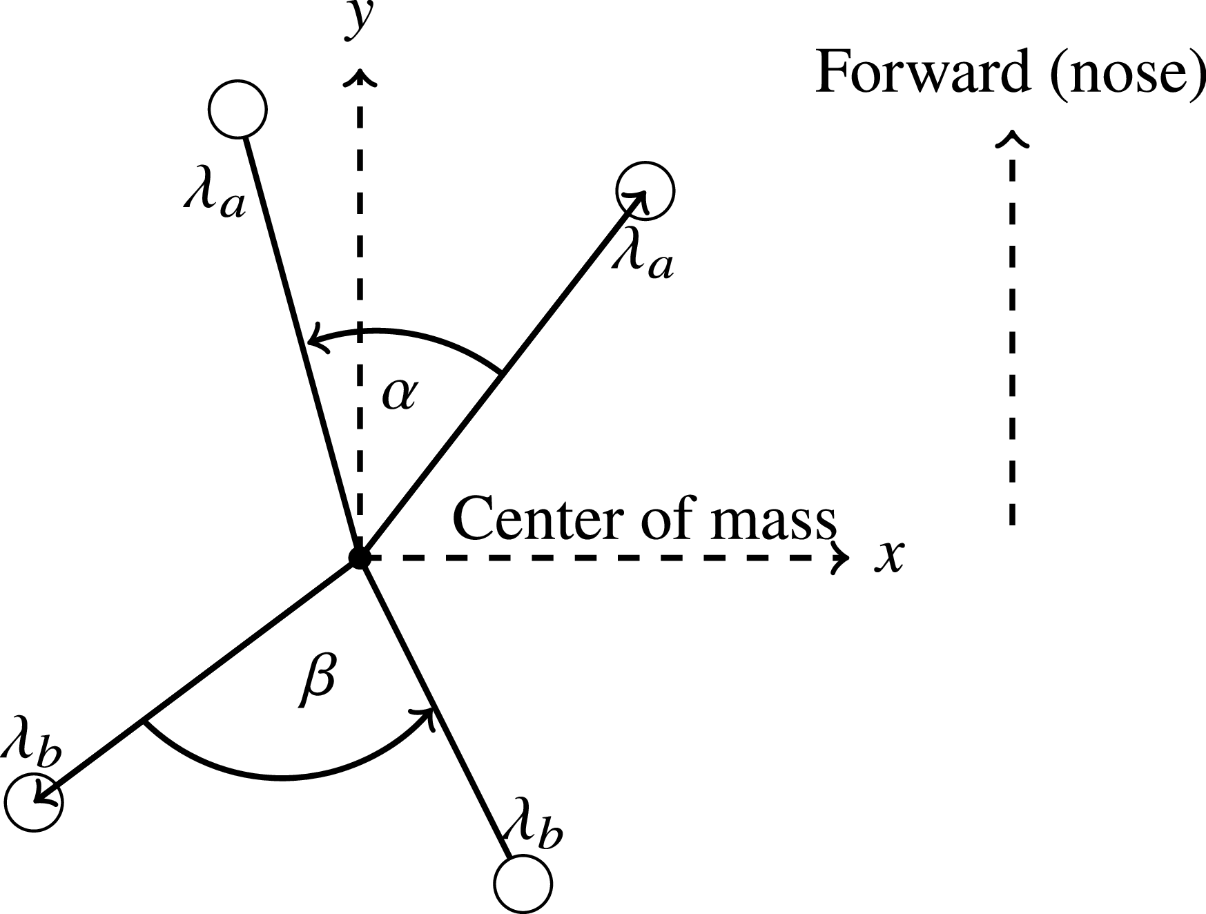

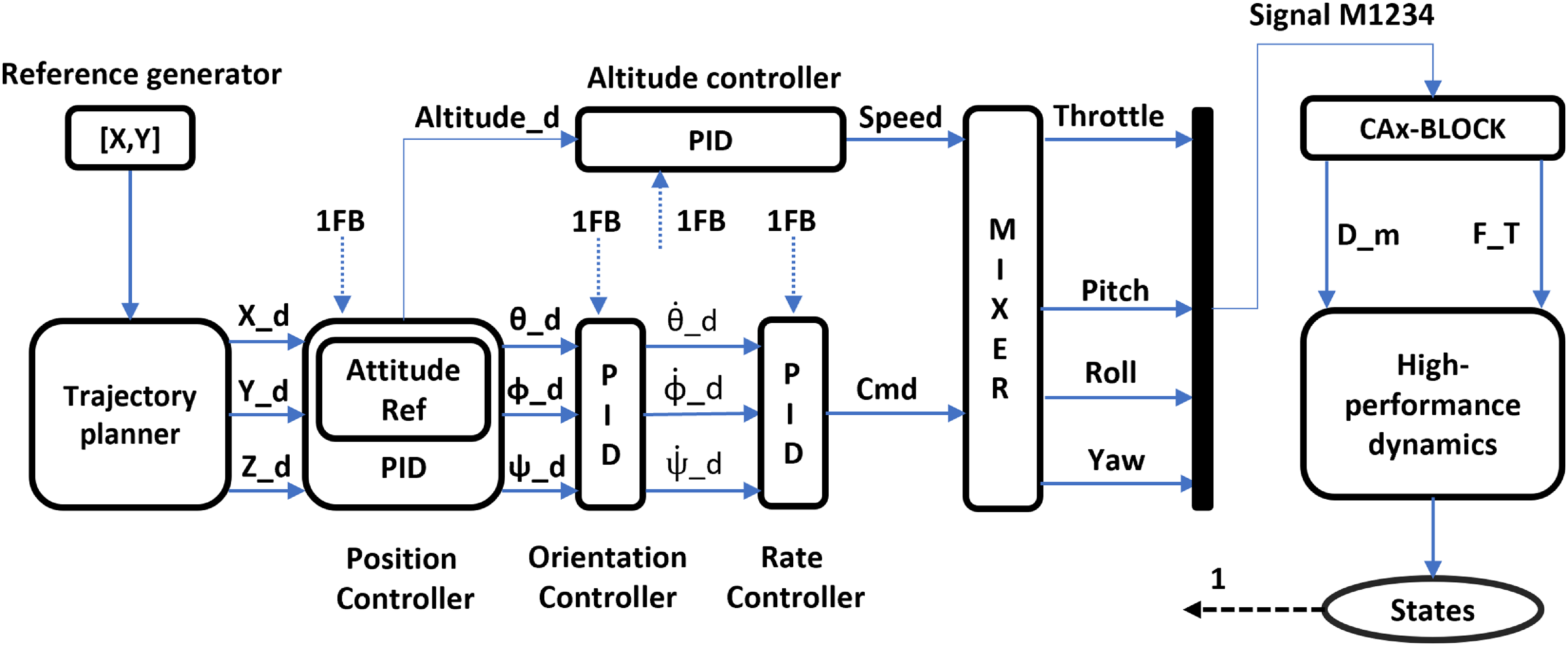
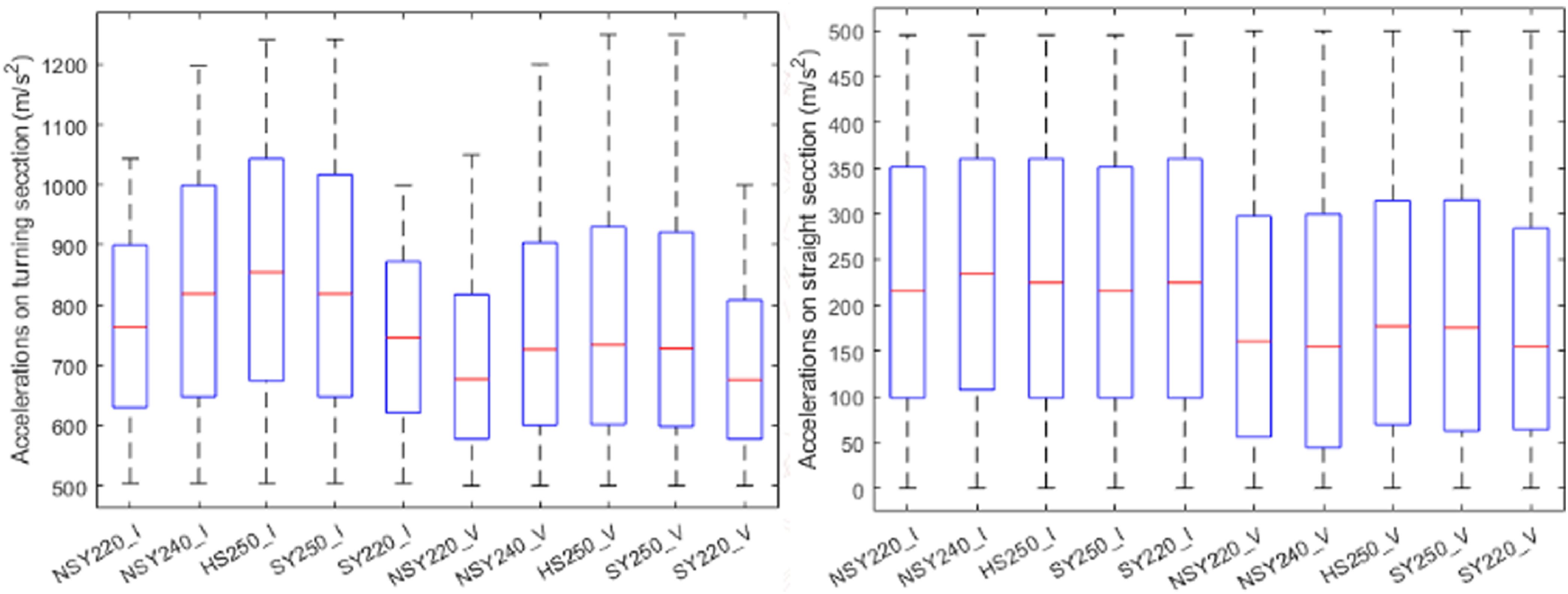
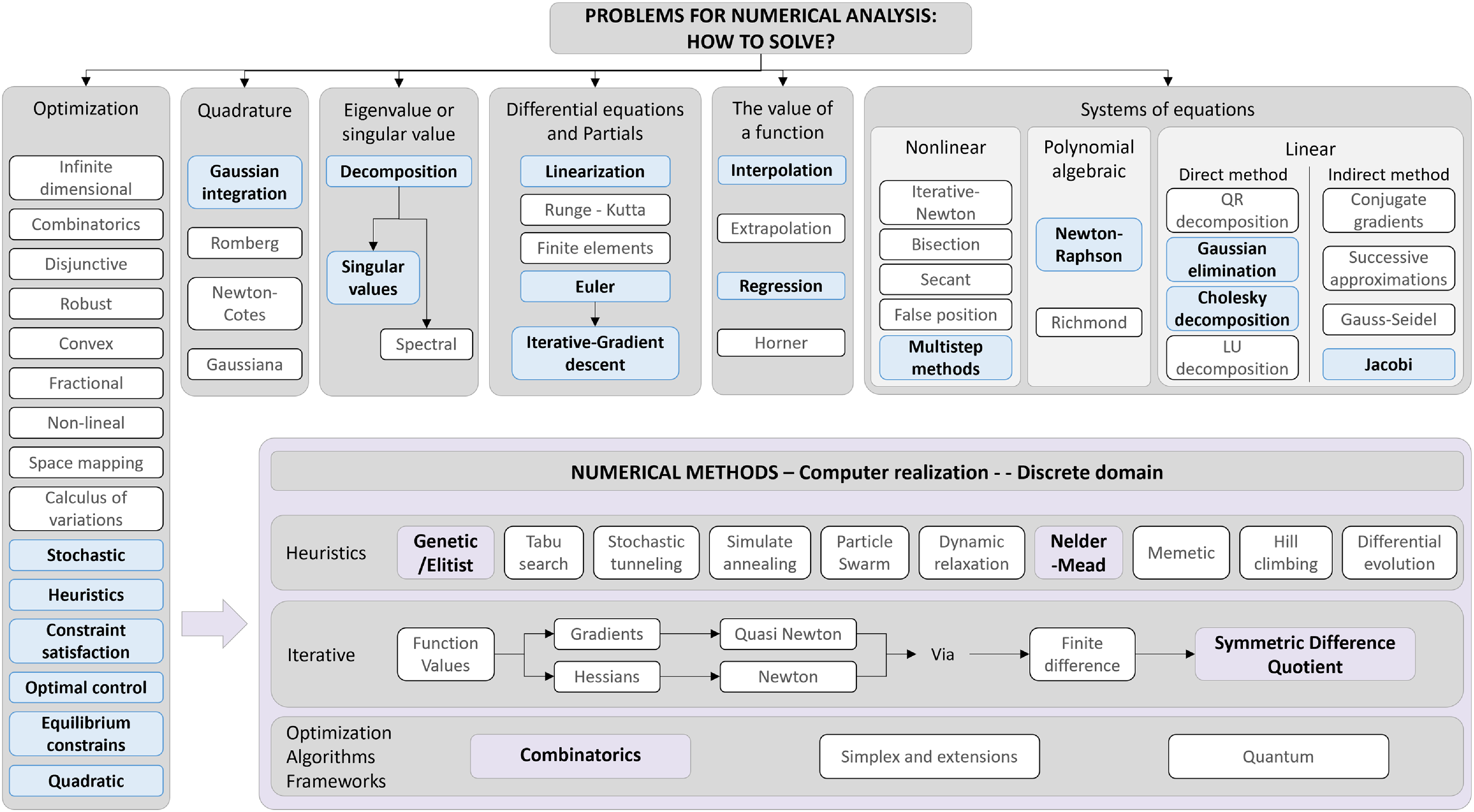
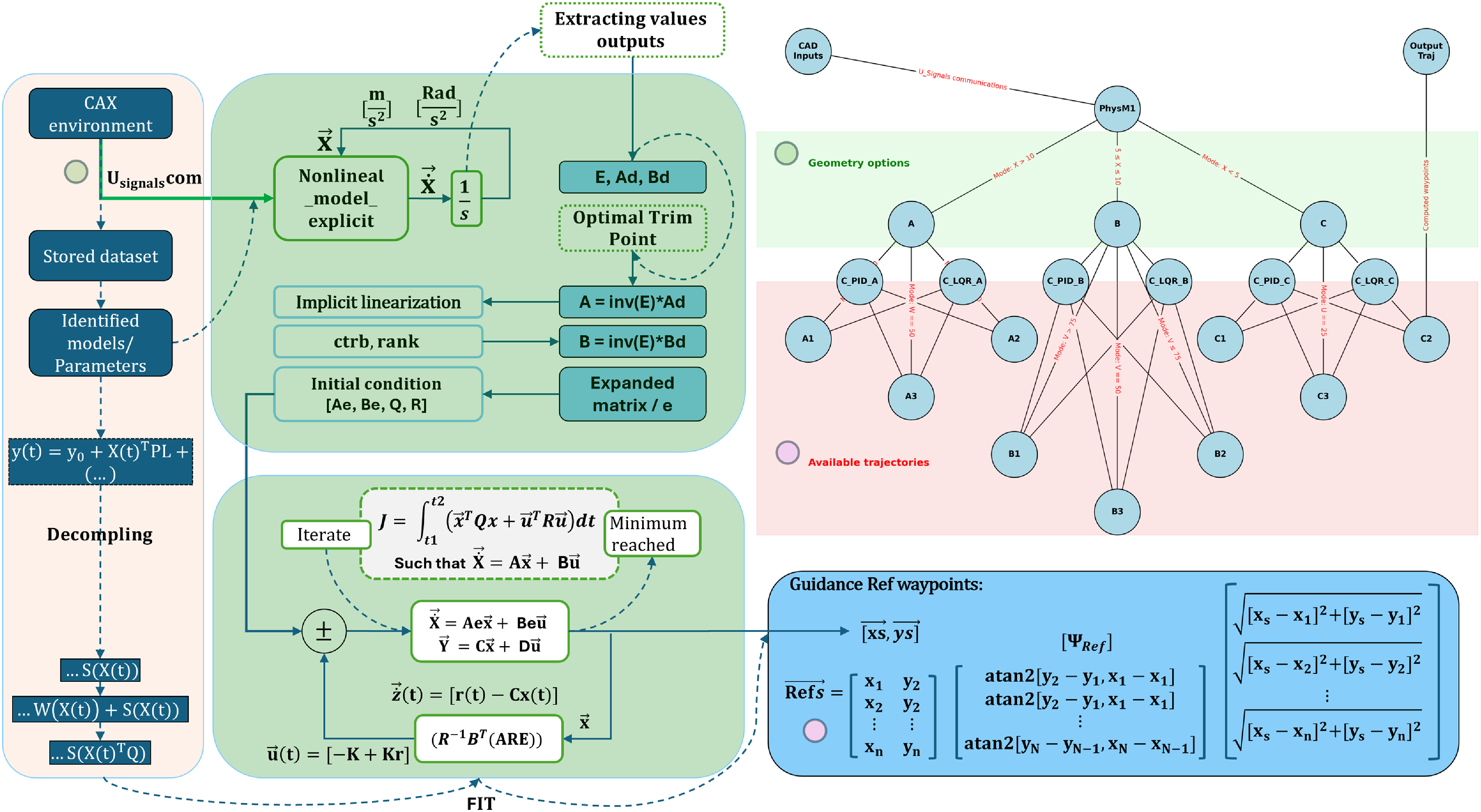
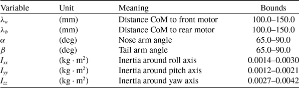
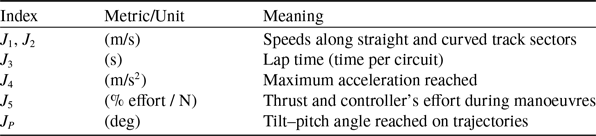
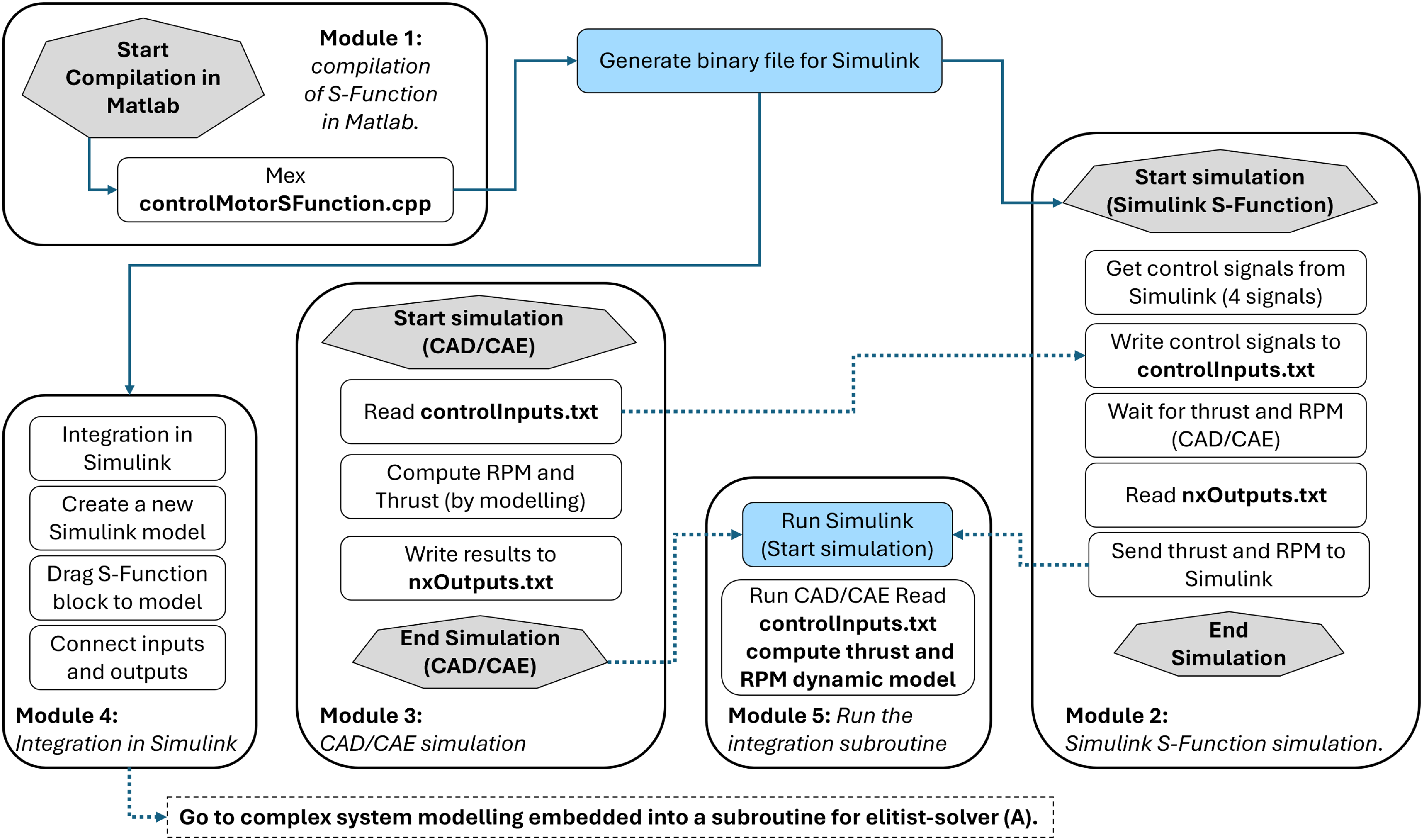
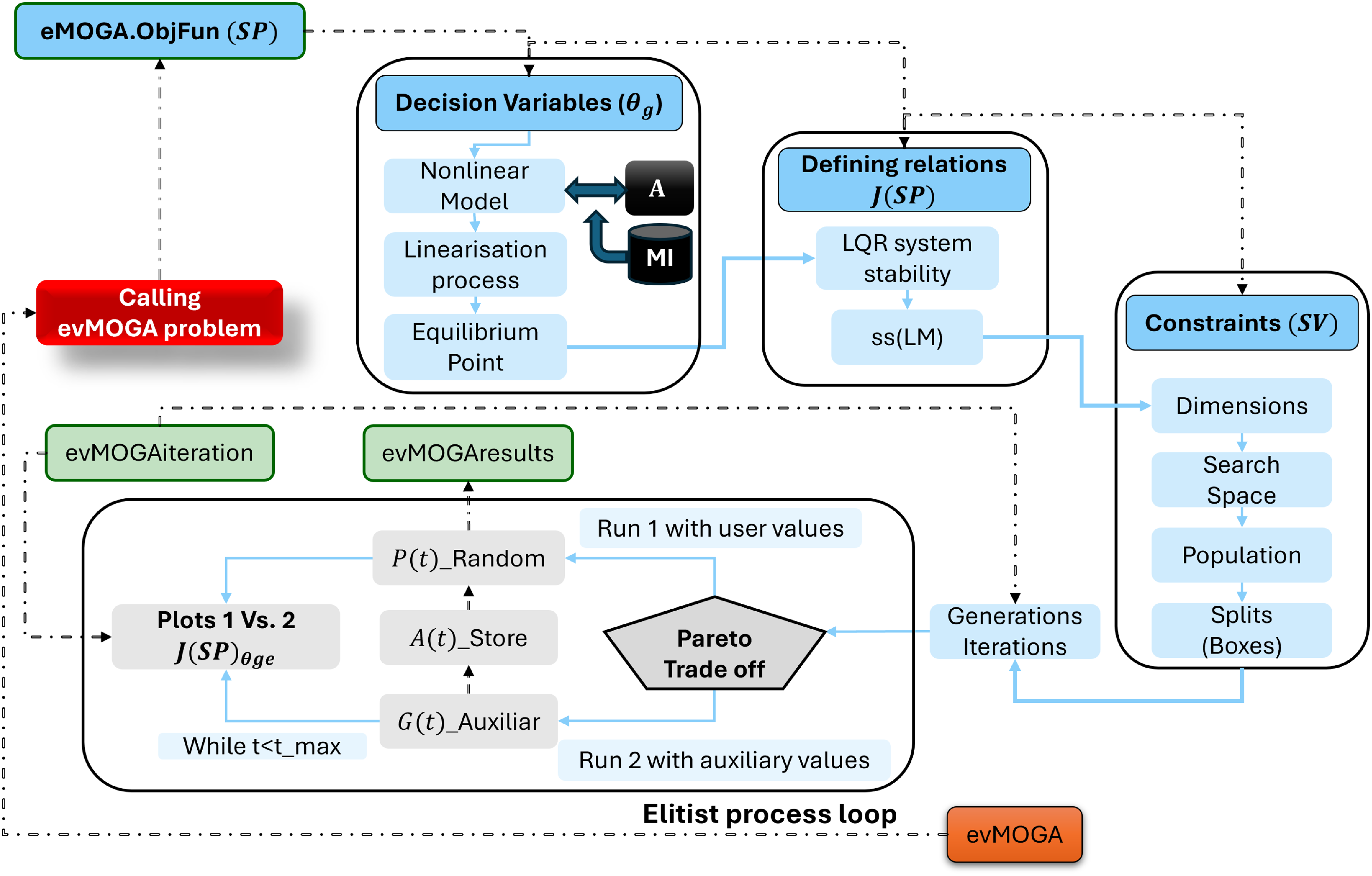
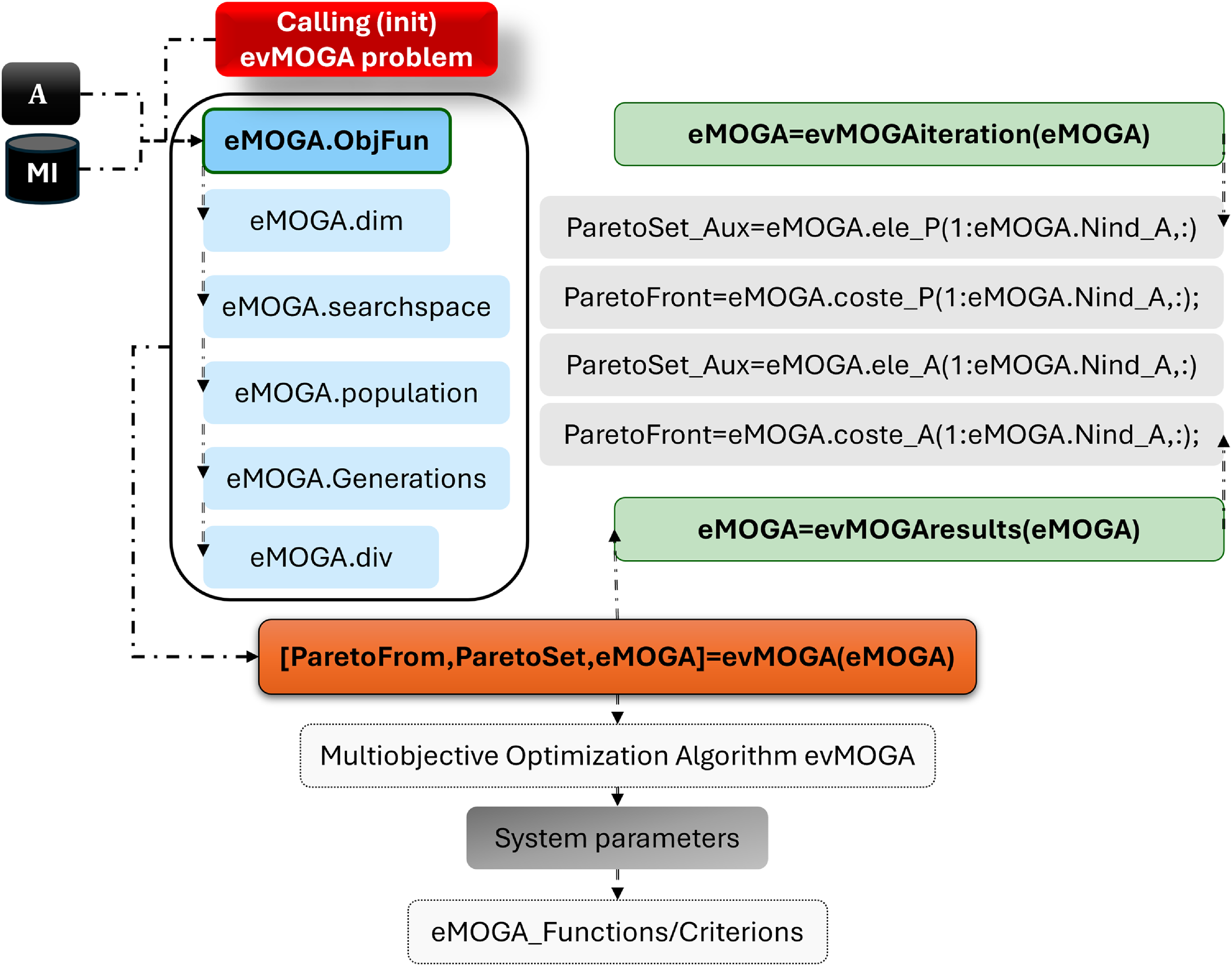
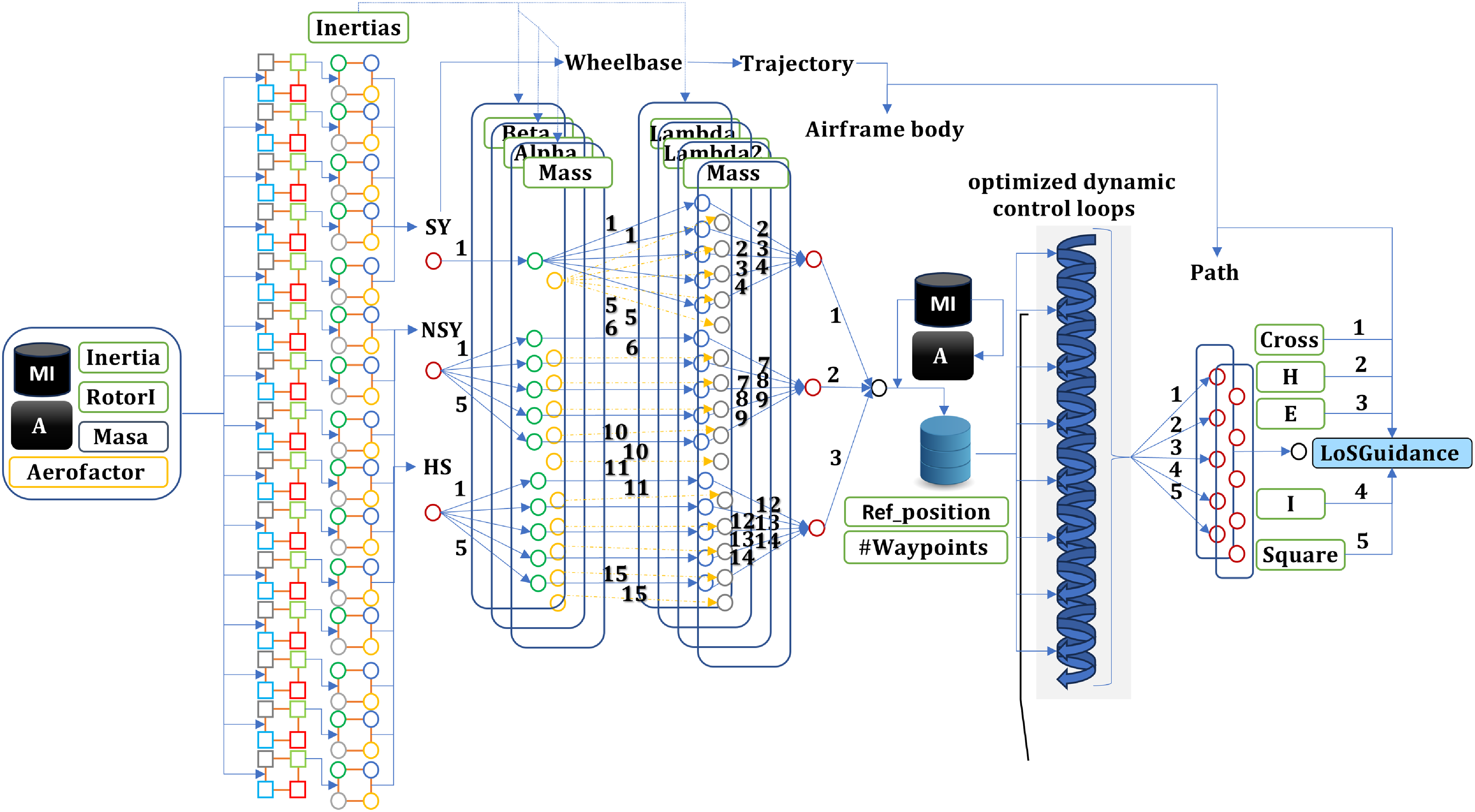


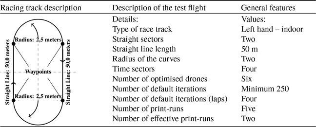
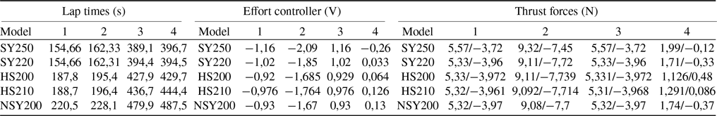
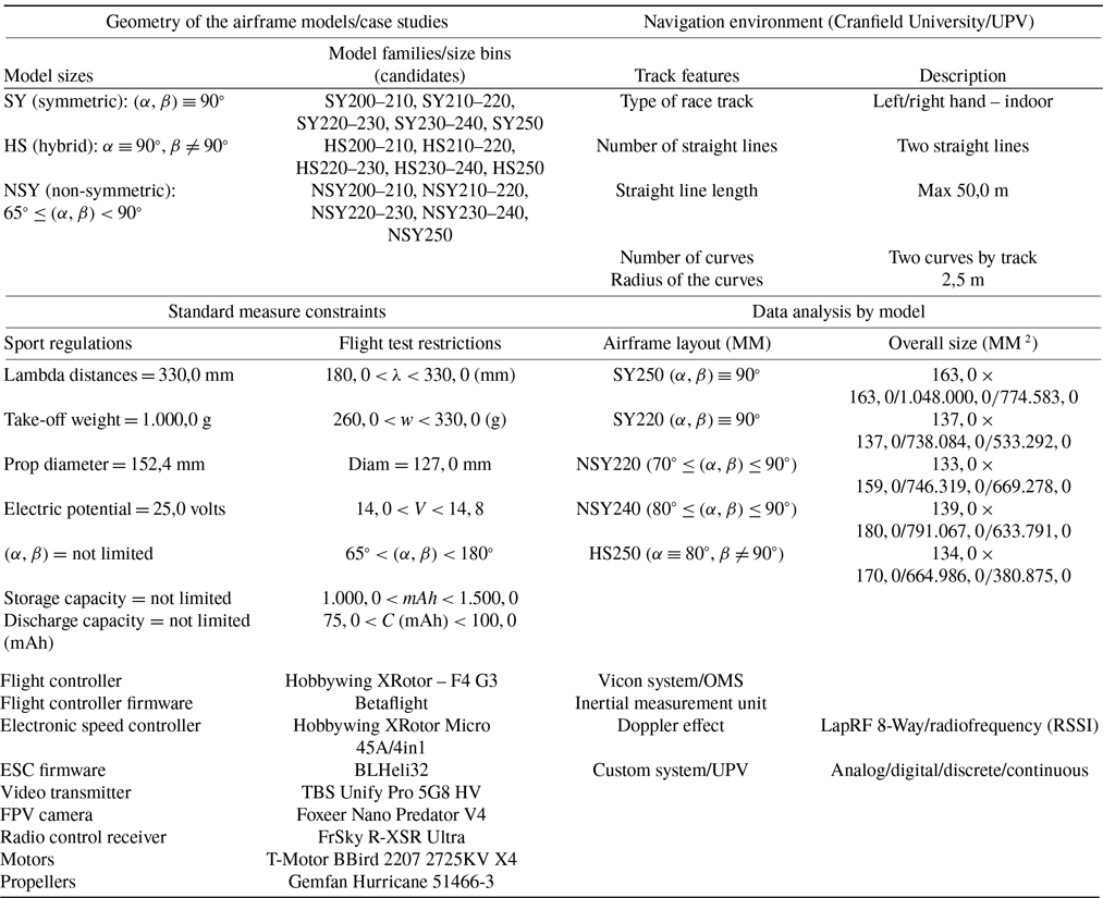
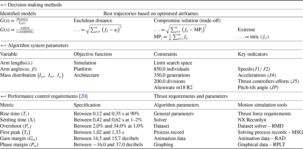
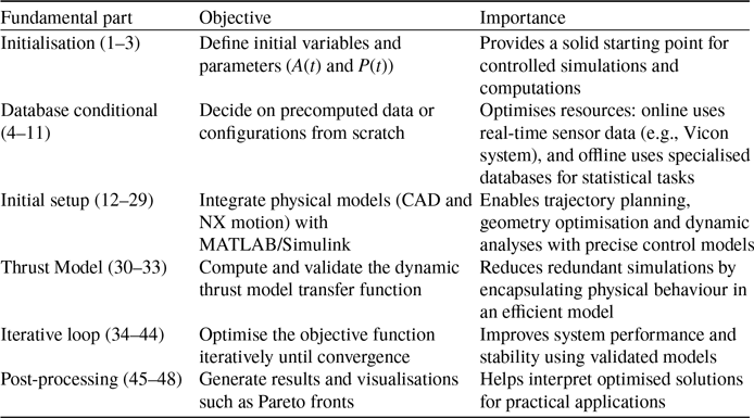
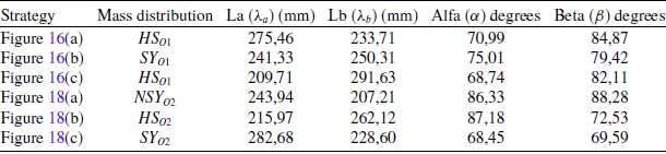
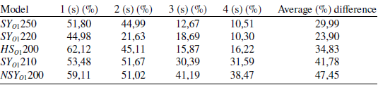
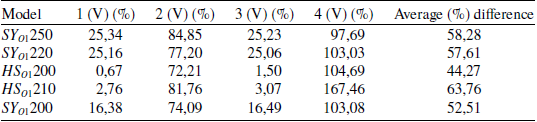
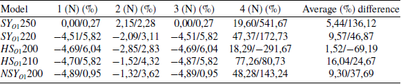
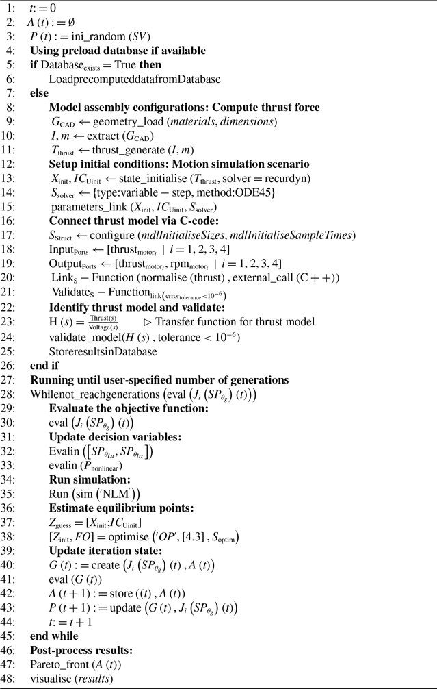


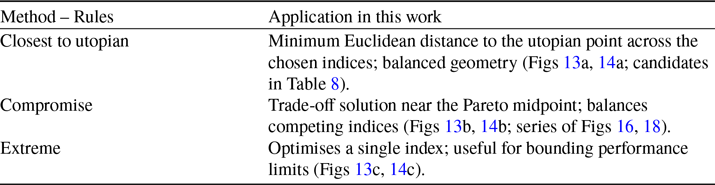

 Open access