2. Stylized facts

Tables 1 and 2 report the mean age at first marriage, averaged over countries within the same region, for the years 1950 to 2004. The raw data appear in Appendix A and the details of its compilation are provided in Appendix B. Averaging over groups of countries allows to summarize the data but also solves the problem of gaps in data at a country level. The average is unweighted, and, thus, is not dominated by large countries. The number of countries in each group is reported in parentheses.

Table 1.

Mean age at first marriage, 1950–2004, men

Note: The table reports unweighted average age at first marriage of men. The raw data are found in Appendix A. The number of countries is reported in parentheses.

Table 2.

Mean age at first marriage, 1950–2004, women

Note: The table reports unweighted average age at first marriage of women. The raw data are found in Appendix A. The number of countries is reported in parentheses.

Summarizing the table, the mean age of marriage decreased in Northern and Central Europe and in Western OffshootsFootnote ⁴ by half a year every decade between 1950 and 1970 and has increased by 1 year every decade since then. The decrease in Southern Europe, Ireland, and Latin America started in the late 1950s and early 1960s and lasted until the late 1970s and early 1980s. In Eastern Europe there was almost no decrease at all and the sharp increase is observed only since the 1990s. It is difficult to draw any conclusions on the trend in Asia and Africa in the first years of the sample because of the small number of countries. For the later years, the sample of Asian and African countries is larger and the trend in age of marriage is upward but the slope is not as sharp as in Europe and the Americas.Footnote ⁵

Figure 1 summarizes the findings by classifying all countries into two groups: Western countries, which include Central and Northern Europe and Western Offshoots, and other countries. The figure leads to three insights. First, the mean age of marriage changes faster in the West than in other parts of the world. This is true for both the decreasing and increasing portions of the U-shape. Second, in the West, age of marriage of men and women is much more strongly correlated than in the rest of the regions. Third, age of marriage of Western women has always been above that of non-Western women, except for the bottom point in the 1960s. For men, the picture is different. Men married older in non-Western countries than in Western ones until the 1970s, but the opposite has been true ever since then.

Figure 1.

Mean age at first marriage.

Note: The figure presents the mean age at first marriage, averaged over countries. Data correspond to Tables 1 and 2. See Appendix A for raw data and Appendix B for details of its compilation. Western countries include Central and Northern Europe and Western Offshoots (United States, Canada, Australia, and New Zealand).

The post-WWII U-shape can be summarized by the following statistics. The unweighted cross-country mean age of marriage of Western women decreased from 23.8 to 22.5 between 1950 and 1965 while that of men decreased from 25.9 to 24.7. Age of marriage increased between 1965 and 2000 to 28.3 for women and 30.1 for men. In non-Western countries age of marriage of women decreased between 1950 and 1965 from 23.3 to 22.6, and increased between 1970 and 2000 to 25.6. For non-Western men, the decrease lasted until 1970 and constituted a drop from 26.3 to 25.3. It was followed by a rise to 27.8 until 2000.

Figure 2 shows the post-WWII mean age at first marriage in Western countries, divided into groups of related or similar countries: Northern Europe, Central Europe, Southern Europe and Ireland, and Western Offshoots. The figure plots different levels of age of marriage and different timing of the U-shape across the West. Western Offshoots had the earliest U-shape, and the turn from the decreasing to the increasing trend took place in the 1960s. By contrast, Southern Europe and Ireland only started to experience the decrease around that time. Western Offshoots had the lowest age of marriage until the 1980s, while age of marriage in Southern Europe and Ireland was the highest. However, after the sharp increase in Western Offshoots between 1960s and 1980s, age of marriage in this group of countries has been higher than in Southern Europe. Northern and Central Europe are close to each other. Similarly to Western Offshoots, Northern and Central Europe turned in the 1960s from decreasing to increasing age of marriage, but they have always had a higher level of age of marriage than Western Offshoots.

Figure 2.

Age of marriage in Western countries: women (left) and men (right).

Note: The figure shows the mean age at first marriage in four groups of Western countries. Data correspond to Tables 1 and 2. See Appendix A for raw data and Appendix B for details of its compilation

3. Relation to economic development

In this section, I provide evidence that the post-WWII marriage age U-shape in Western countries mirrors the post-war converging path of these economies. Figures 3 and 4 show the relationship between age at first marriage and GDP per capita for women and men, respectively.Footnote ⁶ The figures distinguish between Western and other countries, similarly to how it is done in Figure 1. The marriage age U-shape as a function of GDP is much clearer in Western than in other countries. The insight is that the U-shape is a reflection of the development path specific to the post-WWII West. Age of marriage sharply decreases with the industrial boom, and the turnaround from decrease to increase is associated with the later stage of economic development. Western countries vary in the timing of the development path. Correspondingly, they vary in the timing of the marriage age U-shape. For example, at the time that age of marriage in Southern Europe and Ireland started to decrease and the economy to boom, age of marriage in other parts of the Western world already started to increase. This makes the post-WWII decades a special event in economic and demographic history, where one observes a common growth pattern associated with common U-shaped dynamics of age of marriage.

Figure 3.

Age at first marriage and GDP per capita, women.

Note: The figure presents the age at first marriage and log of real GDP per capita. GDP is taken from Maddison (Reference Maddison, van Ark and Crafts1996). Age of marriage corresponds to Tables 1 and 2. The lines are predicted values from a nonparametric kernel regression. See Appendix A for raw data and Appendix B for details of its compilation.

Figure 4.

Age at first marriage and GDP per capita, men.

Note: The figure presents the age at first marriage and log of real GDP per capita. GDP is taken from Maddison (Reference Maddison, van Ark and Crafts1996). Age of marriage corresponds to Tables 1 and 2. The lines are predicted values from a nonparametric kernel regression. See Appendix A for raw data and Appendix B for details of its compilation.

Another perspective on the relationship between age of marriage in the West and post-WWII economic development is illustrated in Figures 5 and 6. These figures show the relationship between overall economic growth and overall change in the age of marriage during the 1960s–1990s period for men and women, respectively. The horizontal axis is the economic growth during the 30 years between 1960–1964 and 1990–1994, and the vertical axis is the corresponding change in the age of marriage (the difference is between the average of the 1990–1994 period and the average of the 1960–1964 period). The figures distinguish between the 15 original European Union countries, other Western countries, and non-Western countries. Across the old European Union, the correlation between overall change in the mean age at first marriage and overall change in the logged per capita GDP during this period is $-0.9$ for both genders. Other Western countries are also located on the same decreasing slope. Nordic countries and the United States are located at the top-left corner of the graph: between the 1960s and the 1990s, age of marriage in these countries rose sharply, but the economic growth was more moderate than in Southern Europe, located at the bottom-left corner.

Figure 5.

Change in the age of marriage and economic growth between early 1960s and early 1990s, women.

Note: The figure presents the change in the age at first marriage, averaged over regions (each country in a region is one observation). The change is between the average over 1960–1964 period and the average over 1990–1994 period. GDP is taken from Maddison (Reference Maddison, van Ark and Crafts1996), and logged after averaging. Age of marriage corresponds to Tables 1 and 2. See Appendix A for raw data and Appendix B for details of its compilation.

Figure 6.

Change in the age of marriage and economic growth between early 1960s and early 1990s, men.

Note: The figure presents the change in the age at first marriage, averaged over regions (each country in a region is one observation). The change is between the average over 1960–1964 period and the average over 1990–1994 period. GDP is taken from Maddison (Reference Maddison, van Ark and Crafts1996), and logged after averaging. Age of marriage corresponds to Tables 1 and 2. See Appendix A for raw data and Appendix B for details of its compilation.

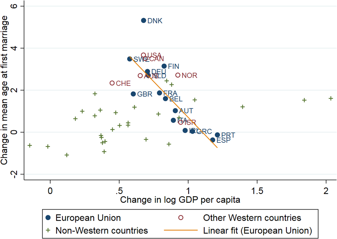
This almost-perfect negative correlation among Western but not other countries shows that the marriage age U-shape is a mirror reflection of the economic convergence path across Western countries. In other words, the fast economic growth during the industrial boom is associated with declining age of marriage, but as growth slows down age of marriage starts to rise. Although the former fast stage is related to the rising productivity in male labor-dominated sectors, the latter slow stage is related to tertiarization of the economy, associated with rising female labor force participation. In the United States, Northern and Central Europe the U-shape started either between the world wars or with the implementation of the Marshall Plan, and in Southern Europe and Ireland it started with the modernization of the economies in the 1960s. For example, in Spain, age of marriage started to decrease in 1962, at precisely the time the Stabilization Plan started to be implemented. Around the same time, the age of marriage in Nordic countries and the United States already turned from the decreasing to the increasing trend.

Some countries are missing from Figures 5 and 6, because of gaps in the marriage age data for the specific years considered in the figures. For a more complete cross-country picture of the relationship between the change in age of marriage and economic growth, I include in Appendix C the corresponding Figures C1 and C2, where countries are grouped into regions. The figures show a clear negative correlation between economic growth over the 1960s–1990s period and the change in age of marriage. Again, some non-Western regions are not located on the negative slope.

Evidence in Figures 5, 6, C1, and C2 is about the timing of the U-shape. It comes first in Northern Europe and Western Offshoots and later in Southern Europe and Ireland. As a result, comparison between 1960s and 1990s shows a strong negative correlation between change in age of marriage and change in GDP per capita: countries that grew the most during this period of time (Southern Europe and Ireland) have the smallest overall change in the age of marriage because of the U-shape phenomenon.

To make sure that the U-shaped relationship between age of marriage and GDP, observed in Figures 3 and 4, is not driven by country or year confounders, I estimate a two-way fixed effect model, where I regress the mean age at first marriage on the log of GDP per capita and its squared term:

(1)$$MA^{g}_{it} = \alpha_{1}^{g}GDP^{2}_{it} + \alpha_{2}^{g}GDP_{it} + \mu^{g}_{i} + \gamma^{g}_{t} + \varepsilon_{it}^{g}$$

where $MA^{g}_{it}$ is the mean age at first marriage of gender $g$ in country $i$ in year $t$. GDP is in real per capita terms and adopted from the Penn World Table [Feenstra et al. (Reference Feenstra, Inklaar and Timmer2015)], which reports GDP from 1950 on. Country and year fixed effects are, respectively, $\mu _i$ and $\gamma _t$. Standard errors are clustered by country.

The results are presented in Table 3. Columns 1 and 2 show the estimation results of equation (1), for men and women, respectively. The quadratic form is statistically significant and follows the U-shaped form. All predicted values are located within the positive quadrant: the predicted age at first marriage is between 24.6 and 30.4 for men and between 21.9 and 27.7 for women. The coefficients of the quadratic equation are different for men and for women. In particular, men experience a sharper change in age of marriage as a function of GDP. However, the GDP level when the U-shape is at its bottom point is similar for both genders: 9.1 log points for men and 9.2 log points for women. These findings explain the heterogeneity in the timing of the U-shape across different Western countries but also similarity across genders. In particular, they provide an economic interpretation of the differences between Western Offshoots, Northern, Central, and Southern Europe, observed in Figure 2.

Table 3.

Age at first marriage and GDP per capita

Note: The table presents results of fixed-effects regressions of equation (1). Standard errors are clustered by country. $^{\ast }p< 0.1$, $^{\ast \ast }p< 0.05$, $^{\ast \ast \ast }p< 0.01$.

4. The U-shape as a special event

A zoom out to a broader historical perspective reveals that the post-WWII marriage age U-shape is a special event in the post-Malthusian history. The uniqueness of the post-WWII marriage age U-shape consists in the strong correlation between Western countries, the correlation between genders, and the strong correlation between the U-shape and the economic development path. By contrast, before WWII the trends in the marriage age in different Western countries were not synchronized. For instance, due to Wrigley et al. (Reference Wrigley, Davies, Schofield and Oeppen1997) and other sources, we can follow the mean age of marriage in England since 1600. Age of marriage decreased for men starting in the late seventeenth century and for women starting in 1700. It started to increase in the early nineteenth century and continued to increase slowly (with a short disturbance) until World War I (WWI). However, it decreased by about 2 years between WWI and 1970 and from then to the turn of the twenty-first century it steeply rose by about 5 years.

Wrigley et al. (Reference Wrigley, Davies, Schofield and Oeppen1997) find that the source of the long-term decrease in age of marriage was driven by the manufacturing-biased parishes of England as early as in the eighteenth century. Furthermore, Grebenik et al. (Reference Grebenik, Rowntree, Carrier, Colombo, Martin and Roberts1963) compare British data from the 1880s to data collected around 1960. They find that in the 1880s, male miners married at age 24, artisans and laborers at 25.5, farmers at 29, and professional men at 31. Age of marriage of men and women in England decreased after WWI and continued to decrease after WWII. However, for couples where the groom was a high-skilled worker (either manual or non-manual) age of marriage decreased by 1 year more than for couples where the groom was a low-skilled worker. This comparison between the 1880s and 1960 reveals the effect of improvement in the skills of English men on age of marriage.

The trend in other Western countries was not always similar to the one in England. Figure 7 presents time series for Western countries with data available since 1800. In Belgium, Denmark, and to a lesser degree France, age of marriage decreased during the nineteenth century. Belgium is a salient case of a steep fall in age of marriage from the extreme level of 30 in 1800. However, the same is not true for the United States, where age of marriage increased during almost all of the nineteenth century. In Germany age of marriage of women decreased starting in the 1930s but that of men decreased only after WWII. In Italy, age of marriage decreased only in the 1960s and 1970s. In contrast to age of marriage in France, England, and Belgium, age of marriage in Sweden increased from the middle of the eighteenth century until the 1930s when it started to decrease. Similarly, the age at first marriage in Switzerland decreased from the 1930s [Schoen and Baj (Reference Schoen and Baj1984)].

Figure 7.

Mean age at first marriage since 1800 in Western countries.

Note: See Appendix B for details of data compilation

Three insights can be taken from these observations. First, before WWII different Western countries followed different trends in age of marriage. In particular, as discussed in Haines (Reference Haines1996), the relatively low age of marriage in the United States during colonial times is associated with the better economic capacity in the American colonies than in Europe. Second, age of marriage in some countries followed a long decreasing trend. This was the case in England in the eighteenth century and in France, Belgium, and Denmark in the nineteenth century. Finally, the starting point of the twentieth century U-shape varies across countries. In the United States the decrease starts around the Second Industrial Revolution. In Sweden, Switzerland, and England it starts after WWI. In Germany, Italy, and (not shown in the figure) Spain, Portugal, and Ireland it starts as late as the 1960s.

5. A model of the post-WWII U-shape

5.2. Setup

5.2.1. Production

Consider an economy that uses labor to produce a single-market good. I assume existence of two technologies. Technology $A$ requires male physical ability, while technology $B$ not.Footnote ⁷ Thus, women use technology $B$, while men use $max\{ A,\; B\}$. For simplicity of notation, I assume that $A> B$, so men use $A$. Each individual is endowed with observed ability $\phi$, distributed in the population with a cumulative distribution function $F( \phi )$. Wages are $A\phi$ and $B \, \phi$, for workers who use technologies $A$ and $B$, respectively.

Women can produce home product instead of labor force participation.Footnote ⁸ The value of home product does not depend on ability and is worth one unit of the market product. The assumption that home product is constant does not contradict home productivity growth. Introduction of appliances makes housework faster and easier and gives housewives more time for leisure [Aguiar and Hurst (Reference Aguiar and Hurst2007)],Footnote ⁹ but the volume of meals to be cooked, space to be cleaned, and clothes to be washed remains unchanged.

5.2.2. Preferences

“It is not good that the man should be alone” (Genesis 2:18), and the utility of singles is zero. Married couples consume their income as a public good. The expected life-time consumption of a just-married couple, where the man has ability $x$ and the woman has ability $y$, is

(2)$$c( x,\; y) = Ax + IBy + 1-I$$

where $I\in \{ 0,\; 1\}$ indicates the wife's labor force participation extensive margin. The term $1-I$ indicates that if she does not work in the market, she produces one unit of home product. The age of marriage does not affect lifetime consumption. Individual preferences are given by a concave function $u( c)$. Let us denote

(3)$$u( x,\; y) \equiv u( c( x,\; y) ) .$$

5.2.3. Labor force participation

Similarly to Greenwood et al. (Reference Greenwood, Seshadri and Yorukoglu2005), all men and single women work in the market. A married woman chooses to work only if her market product is above home product, i.e., if $By> 1$. Let $z = F( {1}/{B})$ indicates the rank of the lowest-ability woman who participates in the labor force after marriage. Let us call “above-$z$” and “below-$z$” individuals ranked above or below $z$ in the ability distribution, respectively. That is, below-$z$ women have ability $y< {1}/{B}$. They do not work after marriage, and they are identical in the sense that they all offer their mates one unit of home production. The above-$z$ women work after marriage, and their market ability is distributed $F( y\vert y> {1}/{B})$.

5.2.4. Marriage market

Finite equal numbers of men and women enter the economy each period and participate in the marriage market for up to two periods.

5.2.4.1. First period

The first period can be intuitively titled “high school” period, when all men and women are single and gather together at school or in the neighborhood of residence. All men and women sort into random couples. The man can choose to propose marriage and the woman can accept or reject the offer.

5.2.4.2. Second period

The second period can be intuitively titled “college” or “work” period. In this period, individuals are exogenously sorted according to ability, because college and industry design interactions between individuals with similar level of skills. Therefore, with probability one, men meet women of the same level of ability, means $x = y$, whenever the corresponding woman is single or above-$z$ married. A man can propose marriage if he and his female mate are single, and the woman can accept or reject the offer.

6. Supportive evidence

In this section, I use the Current Population Survey [CPS, Flood et al. (Reference Flood, King, Rodgers, Ruggles and Warren2020)] data from the United States to test the main model's prediction, captured in Proposition 2, i.e., that “male” sectors productivity is negatively affecting age of marriage. I estimate the following model:

(5)$$S( a,\; g) _{ist} = \alpha_{1}M_{st} + X_{ist}\beta + \gamma_{s} + \eta_{t} + \varepsilon_{ist}$$

where $S( a,\; g) _{ist}$ is a dummy for being never-married at age $a$. The unit of observation is individual $i$ of gender $g$, who lives in state $s$ and was 18 years old in year $t$.

The main explanatory variable $M$ is the labor productivity in the “male” sector. Below I explain in detail the construction of this variable and the identification assumption. The state and year fixed effects are $\gamma _{s}$ and $\eta _{t}$, respectively. $X$ is a set of controls. It includes a dummy for whites and the following state-level variables: four variables for the minimal legal age of marriage (minimal for men and for women, with and without parental consent), a dummy for early legal access, i.e., availability of oral contraception for single childless women below age 21 [from Bailey et al. (Reference Bailey, Guldi, Davido and Buzuvis2012)], a dummy for the possibility of no-fault divorce [from Vlosky and Monroe (Reference Vlosky and Monroe2002)], and a dummy for legal abortion [from Levine et al. (Reference Levine, Staiger, Kane and Zimmerman1999)]. Standard errors are clustered by state.

6.1. Identification strategy

I seek an explanatory variable that accounts for productivity in the “male” sector with respect to the weight of this sector in each state's economy. The problem is that the dynamics of each state's economic structure is endogenous. In order to identify the effect of “male” sector labor productivity, I propose to fix the initial conditions in each state and use them as weights of the industries in the state's economy. The change over time comes from country-level productivity growth, but the variation across states comes from different initial conditions.

Identification assumption: The country-level labor productivity is exogenous to each state's initial economic structure.

In other words, I assume that states are small relatively to the whole country, so each state's initial conditions do not determine country-level productivity growth. Therefore, only the differences between the states’ initial conditions allow identification: had all the states the same initial conditions, year fixed effects would absorb any variation over time.

I use this identification assumption to define the main explanatory variable $M_{st}$:

(6)$$M_{st} = \sum_{k = 1}^{K}w_{sk}y_{tk}I_{k}^{m}$$

where $k$ is the index of an industry out of the total of $K$ industries. First, $w_{sk}$ generates across-state variation by accounting for the state's initial economic structure. Specifically, it is the initial $k$'s weight in the state $s$ output. I use Renshaw et al. (Reference Renshaw, Trott and Friedenberg1988), who provide state-level decomposition of output by industry from 1963 on. I use the first years of these data, i.e., 1963–1965, to calculate the weights $w_{sk}$. Second, $y_{tk}$ generates over-time variation by accounting for country-level per-worker output in industry $k$ in year $t$:

(7)$$y_{tk} = {Y_{tk}\over L_{tk}}$$

where $Y_{tk}$ is industry $k$ country-level output and $L_{tk}$ is the industry's number of workers in year $t$. These data come from Dale Jorgenson's KLEMS project.Footnote ¹² I convert the data into thousands of inflation-adjusted 1980 dollars.

Finally, $I_{k}^{m}$ is a binary indicator for being the industry “male.”Footnote ¹³ “Male” industry is composed of more than 70% male workers among 25–34 year old workers according to the American Census of 1990 [Steven et al. (Reference Steven, Katie, Ronald, Josiah and Matthew2017)]. By this definition, the male sectors are agriculture, mining, construction, and durable goods manufacturing. This retrospective definition with respect to the gender shares in 1990 is aimed at identification of sectors that remained dominated by male workers despite the increased female labor force participation.Footnote ¹⁴

6.2. Results

Panel A of Table 4 presents the results of estimation of equation (5). I estimate the model eight times: for men and women, separately for samples of individuals who are at least 21, 23, 25, and 27 years old. The results plot a robust statistically significant negative coefficient of the male sector in line with the model's predictions: a negative effect of the male sector on probability of singlehood.

Table 4.

Male sector effect on singlehood and heterogeneity of the effect

Note: The table presents the results of OLS regressions of equation (5). All regressions control for minimal legal age of marriage, include year and state fixed effects, and control for whites, legalization of divorce, abortion, and early access to oral contraception. Standard errors are clustered by state. $^{\ast }p< 0.1$, $^{\ast \ast }p< 0.05$, $^{\ast \ast \ast }p< 0.01$.

CPS data have been collected since 1962, during the period of increasing age of marriage. Nevertheless, I document the negative effect of the male sector on age of marriage in CPS data. Furthermore, in order to test whether the male sector affected age of marriage even by the end of the twentieth century, I estimate the model separately for the years 1962–1989 and 1990–1999. The results of these two estimations appear in panels B and C of Table 4, respectively. The negative coefficient of the male sector is of a higher magnitude in the 1962–1989 period, especially for women. However, it is negative and statistically significant also in the 1990–1999 period. Overall, given that the mean value of the explanatory variable $M$ increased from 14 to 22 in the 1962–1989 period and from 22 to 27 in the 1990–1999 period, the estimation results suggest that the age of marriage in 1999 was 1 year lower than it should be if the male sector productivity had not increased since the 1960s.