


1. Introduction
Pulsars are highly polarised radio sources which have long been used as tools to probe magneto-ionised plasma in the Milky Way and the Local Bubble (e.g. Manchester Reference Manchester1972; Bhat, Gupta, & Rao 1998), the solar wind (e.g. You et al. Reference You, Coles, Hobbs and Manchester2012; Howard et al. Reference Howard, Stovall, Dowell, Taylor and White2016), and the terrestrial ionosphere (e.g. Sotomayor-Beltran et al. Reference Sotomayor-Beltran2013; Porayko et al. Reference Porayko2019). Propagation through the ionised intervening media imparts frequency-dependent distortions on pulsar signals which can be precisely measured due to the short intrinsic timescales and broadband nature of the signals. Of particular interest are the cold-plasma dispersion and Faraday rotation effects on the received pulsar signal, characterised by the dispersion measure (DM) and rotation measure (RM), respectively. Together, these quantities contain information about the thermal electron density and magnetic field strength along the line of sight. In fact, pulsar observations are exceptionally useful for studying the magneto-ionised interstellar medium (ISM), including the supernova remnants (SNRs) surrounding young pulsars such as the Vela pulsar (e.g. Hamilton et al. Reference Hamilton, McCulloch, Ables and Komesaroff1977; Hamilton, Hall, & Costa Reference Hamilton, Hall and Costa1985) and the Crab pulsar (e.g. Rankin et al. Reference Rankin, Campbell, Isaacman and Payne1988).
There are three standard methods for determining the strength of the magnetic field in the ISM. Zeeman splitting of spectral lines provides both the strength and direction of the magnetic field; however, it is only observable for relatively strong magnetic fields in Hi regions or cold, dense molecular clouds (e.g. Heiles Reference Heiles1976, Reference Heiles1989). Alternatively, one can determine the magnetic field strength from the intensity of synchrotron emission, which typically requires making an assumption such as equipartition between the energy density of cosmic ray particles and that of the magnetic field (e.g. Beck & Krause Reference Beck and Krause2005; Arbutina et al. Reference Arbutina, Urošević, Andjelić, Pavlović and Vukotić2012; Urošević, Pavlović, & Arbutina Reference Urošević, Pavlović and Arbutina2018). Although the equipartition method is useful when the available data are limited, it is biased towards areas with strong magnetic fields, which leads to estimates which are higher than average (Beck et al. Reference Beck, Shukurov, Sokoloff and Wielebinski2003). Lastly, the magnetic field strength can also be inferred from the Faraday rotation of linearly polarised emission, such as from synchrotron sources or pulsars. Using pulsar observations, the mean magnetic field strength parallel to the line of sight is simply
 \begin{equation} \langle B_\parallel \rangle \simeq \mathcal{C}^{-1}\frac{\mathrm{RM}}{\mathrm{DM}},\end{equation}
where
 $\mathcal{C}^{-1}\approx 1.232\,\mu\mathrm{G}$
and the RM and DM are in their conventional units (
$\mathcal{C}^{-1}\approx 1.232\,\mu\mathrm{G}$
and the RM and DM are in their conventional units (
 $\mathrm{rad}\,\mathrm{m}^{-2}$
and
$\mathrm{rad}\,\mathrm{m}^{-2}$
and
 $\mathrm{cm}^{-3}\,\mathrm{pc}$
, respectively). A positive
$\mathrm{cm}^{-3}\,\mathrm{pc}$
, respectively). A positive
 $\langle B_\parallel \rangle$
indicates that the magnetic field is, on average, pointing towards the observer. This method is biased towards the warm ionised ISM and can also be biased if small-scale fluctuations in the magnetic field and the electron density are correlated (Beck et al. Reference Beck, Shukurov, Sokoloff and Wielebinski2003). However, pulsar observations still provide a relatively accurate way to estimate the line-of-sight magnetic field strength in almost any direction, which makes it possible to map the large-scale structure of the Galactic magnetic field (e.g. Manchester Reference Manchester1974; Han et al. Reference Han, Manchester and Lyne2006, Reference Han, Manchester and van Straten2018; Sobey et al. Reference Sobey2019).
$\langle B_\parallel \rangle$
indicates that the magnetic field is, on average, pointing towards the observer. This method is biased towards the warm ionised ISM and can also be biased if small-scale fluctuations in the magnetic field and the electron density are correlated (Beck et al. Reference Beck, Shukurov, Sokoloff and Wielebinski2003). However, pulsar observations still provide a relatively accurate way to estimate the line-of-sight magnetic field strength in almost any direction, which makes it possible to map the large-scale structure of the Galactic magnetic field (e.g. Manchester Reference Manchester1974; Han et al. Reference Han, Manchester and Lyne2006, Reference Han, Manchester and van Straten2018; Sobey et al. Reference Sobey2019).
Stochastic fluctuations in RM and DM due to turbulence in the ISM are expected to be of the order
 $10^{-5}$
–
$10^{-5}$
–
 $10^{-4}$
 $\mathrm{rad}\,\mathrm{m}^{-2}$
for observing campaigns of
$\mathrm{rad}\,\mathrm{m}^{-2}$
for observing campaigns of
 $\sim$
1–5 yr (Porayko et al. Reference Porayko2019). This is below the sensitivity of current pulsar monitoring campaigns due to the noise floor set by models of the ionospheric RM contribution. However, it is still possible to study long-term deterministic trends in RM and DM, which can arise for a number of reasons. Linear trends are often observed due to the transverse motion of the pulsar, which causes the line of sight to probe different regions of the ISM at different times (e.g. Backer et al. Reference Backer, Hama, van Hook and Foster1993; Hobbs et al. Reference Hobbs, Lyne, Kramer, Martin and Jordan2004; You et al. Reference You2007; Yan et al. Reference Yan2011; Jones et al. Reference Jones2017;Wahl et al. Reference Wahl2022; Keith et al. Reference Keith2024). Additionally periodic variations on a
$\sim$
1–5 yr (Porayko et al. Reference Porayko2019). This is below the sensitivity of current pulsar monitoring campaigns due to the noise floor set by models of the ionospheric RM contribution. However, it is still possible to study long-term deterministic trends in RM and DM, which can arise for a number of reasons. Linear trends are often observed due to the transverse motion of the pulsar, which causes the line of sight to probe different regions of the ISM at different times (e.g. Backer et al. Reference Backer, Hama, van Hook and Foster1993; Hobbs et al. Reference Hobbs, Lyne, Kramer, Martin and Jordan2004; You et al. Reference You2007; Yan et al. Reference Yan2011; Jones et al. Reference Jones2017;Wahl et al. Reference Wahl2022; Keith et al. Reference Keith2024). Additionally periodic variations on a
 $\sim$
1 yr timescale can arise due to the line of sight probing the solar wind, particularly for pulsars at low solar latitudes (e.g. Jones et al. Reference Jones2017; Wahl et al. Reference Wahl2022; Tiburzi et al. Reference Tiburzi2021). Detailed characterisation of these trends is important for reducing red noise in long-term pulsar timing experiments, which is necessary in order to detect the stochastic gravitational wave background (e.g. Reardon et al. Reference Reardon2023; Agazie et al. Reference Agazie2023).
$\sim$
1 yr timescale can arise due to the line of sight probing the solar wind, particularly for pulsars at low solar latitudes (e.g. Jones et al. Reference Jones2017; Wahl et al. Reference Wahl2022; Tiburzi et al. Reference Tiburzi2021). Detailed characterisation of these trends is important for reducing red noise in long-term pulsar timing experiments, which is necessary in order to detect the stochastic gravitational wave background (e.g. Reardon et al. Reference Reardon2023; Agazie et al. Reference Agazie2023).
Correlated variations in the measured RM and DM can arise when compact regions of magnetised plasma move through the line of sight. As demonstrated by Hamilton et al. (Reference Hamilton, McCulloch, Ables and Komesaroff1977) and Hamilton, Hall, & Costa (Reference Hamilton, Hall and Costa1985), the mean magnetic field strength in the time-varying region can be estimated from the gradients of the two measures:
 \begin{equation} \langle B_\parallel \rangle_\mathrm{var} \simeq \mathcal{C}^{-1}\left(\frac{\mathrm{dRM}}{\mathrm{d}t}\right)\left(\frac{\mathrm{dDM}}{\mathrm{d}t}\right)^{-1},\end{equation}
where
 $\mathcal{C}^{-1}$
is as defined in equation (1). Using observations of the Vela pulsar over
$\mathcal{C}^{-1}$
is as defined in equation (1). Using observations of the Vela pulsar over
 $\sim$
15 yr, Hamilton, Hall, & Costa (Reference Hamilton, Hall and Costa1985) calculated
$\sim$
15 yr, Hamilton, Hall, & Costa (Reference Hamilton, Hall and Costa1985) calculated
 $\langle B_\parallel \rangle_\mathrm{var}=22\,\mu\mathrm{G}$
, which the authors attribute to a magnetised filament in the Vela SNR moving out of the line of sight.
$\langle B_\parallel \rangle_\mathrm{var}=22\,\mu\mathrm{G}$
, which the authors attribute to a magnetised filament in the Vela SNR moving out of the line of sight.
 $\langle B_\parallel \rangle_\mathrm{var}$
has also been estimated for the Crab pulsar (
$\langle B_\parallel \rangle_\mathrm{var}$
has also been estimated for the Crab pulsar (
 $170\,\mu\mathrm{G}$
; Rankin et al. Reference Rankin, Campbell, Isaacman and Payne1988) and several other pulsars (see e.g. van Ommen et al. Reference van Ommen, D’Alessandro, Hamilton and McCulloch1997; Yan et al. Reference Yan2011). More recently, Xue (Reference Xue2019) analysed
$170\,\mu\mathrm{G}$
; Rankin et al. Reference Rankin, Campbell, Isaacman and Payne1988) and several other pulsars (see e.g. van Ommen et al. Reference van Ommen, D’Alessandro, Hamilton and McCulloch1997; Yan et al. Reference Yan2011). More recently, Xue (Reference Xue2019) analysed
 $\sim$
50 yr of historical RM and DM measurements towards the Vela pulsar and identified three separate monotonic trends in the RM: increasing between 1970–1984, decreasing between 1984–2006, then again increasing between 2006–2019. Meanwhile, the DM monotonically decreased over this period, with a flattening in the gradient around 1995 as reported by Petroff et al. (Reference Petroff, Keith, Johnston, van Straten and Shannon2013). From equation (2), these findings imply that the mean line-of-sight magnetic field through the filament underwent two reversals during this time period. Xue (Reference Xue2019) suggested that this could be explained by an inhomogeneous magnetic field within the filament. Given that the Vela pulsar is embedded in a region of turbulent plasma with an apparently inhomogeneous magnetic field, we expect that there may be measurable structure on shorter timescales than what has already been observed, that is, months to years.
$\sim$
50 yr of historical RM and DM measurements towards the Vela pulsar and identified three separate monotonic trends in the RM: increasing between 1970–1984, decreasing between 1984–2006, then again increasing between 2006–2019. Meanwhile, the DM monotonically decreased over this period, with a flattening in the gradient around 1995 as reported by Petroff et al. (Reference Petroff, Keith, Johnston, van Straten and Shannon2013). From equation (2), these findings imply that the mean line-of-sight magnetic field through the filament underwent two reversals during this time period. Xue (Reference Xue2019) suggested that this could be explained by an inhomogeneous magnetic field within the filament. Given that the Vela pulsar is embedded in a region of turbulent plasma with an apparently inhomogeneous magnetic field, we expect that there may be measurable structure on shorter timescales than what has already been observed, that is, months to years.
The SKA-Low will be the most sensitive low-frequency telescope ever built, enabling studies of nearly the entire Galactic pulsar population (e.g. Keane et al. Reference Keane2015). In preparation for the construction of the SKA-Low, several prototype ‘stations’ have been deployed at Inyarrimanha Ilgari Bundara, CSIRO’s Murchison Radio-astronomy Observatory (MRO), to assist with engineering development. In this paper, we aim to use one of these stations, the Aperture Array Verification System 2 (AAVS2), to search for temporal changes on timescales of months to years which could arise from magneto-ionic microstructure in the Vela SNR. Additionally, verification of the prototype station polarimetry will be essential for gaining confidence in polarimetric data obtained with the SKA-Low, and analysis of pulsar observations can be an effective way of achieving this (e.g. Xue et al. Reference Xue, Ord, Tremblay, Bhat, Sobey, Meyers, McSweeney and Swainston2019). The remainder of this paper is organised as follows. In Section 2, we describe the telescope, source selection, observations, and data reduction. In Section 3, we describe the methods used to estimate the RM and DM. In Section 4, we present the results, including polarimetric pulse profiles and the RM and DM measurements. We use these results to validate the station polarimetry and test ionospheric models. In Section 5, we compare the results with historical data and discuss implications for future low-frequency monitoring science. Finally, in Section 6, we summarise and present our conclusions.
2. Observations and data reduction
All observations were collected with the AAVS2 (van Es et al. Reference van Es, Marshall, Spyromilio and Usuda2020; Macario et al. Reference Macario2022), a prototype SKA-Low station consisting of 256 dual polarised log-parabolic antennas pseudo-randomly distributed over a circular ground plane with a diameter of
 $\sim$
42 m and a maximum baseline of
$\sim$
42 m and a maximum baseline of
 $\sim$
38 m. The AAVS2 operates in the frequency range 50–350 MHz and records
$\sim$
38 m. The AAVS2 operates in the frequency range 50–350 MHz and records
 $\sim$
925.926 kHz wide coarse channels separated by
$\sim$
925.926 kHz wide coarse channels separated by
 $\sim$
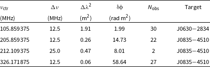
781.25 kHz in order to avoid the drop in sensitivity towards the edges of the bandpass response. The initial AAVS2 system was only capable of recording data from a single coarse channel at a time, but nevertheless was used to detect 20 pulsars at various frequencies (Lee et al. Reference Lee, Bhat, Sokolowski, Swainston, Ung, Magro and Chiello2022). In early 2022, the AAVS2 received an upgrade which enabled it to record data from multiple contiguous coarse channels. Although in principle this upgrade enables the simultaneous recording of an arbitrary number of channels, the practical limit is set by the maximum possible data recording rate. In this work, we recorded contiguous frequency bands with 16 and 32 channels, corresponding to instantaneous bandwidths of 12.5 and 25 MHz, respectively. In Table 1, we summarise the frequency setups used and their corresponding effective resolutions in Faraday space as defined in equation (8).
$\sim$
781.25 kHz in order to avoid the drop in sensitivity towards the edges of the bandpass response. The initial AAVS2 system was only capable of recording data from a single coarse channel at a time, but nevertheless was used to detect 20 pulsars at various frequencies (Lee et al. Reference Lee, Bhat, Sokolowski, Swainston, Ung, Magro and Chiello2022). In early 2022, the AAVS2 received an upgrade which enabled it to record data from multiple contiguous coarse channels. Although in principle this upgrade enables the simultaneous recording of an arbitrary number of channels, the practical limit is set by the maximum possible data recording rate. In this work, we recorded contiguous frequency bands with 16 and 32 channels, corresponding to instantaneous bandwidths of 12.5 and 25 MHz, respectively. In Table 1, we summarise the frequency setups used and their corresponding effective resolutions in Faraday space as defined in equation (8).
AAVS2 frequency bands used in this work. The columns (from left to right) are: the centre frequency (
 $\nu_\mathrm{ctr}$
), the bandwidth (
$\nu_\mathrm{ctr}$
), the bandwidth (
 $\Delta\nu$
), the span in
$\Delta\nu$
), the span in
 $\lambda^2$
(
$\lambda^2$
(
 $\Delta\lambda^2$
), the Faraday depth resolution (
$\Delta\lambda^2$
), the Faraday depth resolution (
 $\unicode{x03B4}\unicode{x03D5}$
; see equation 8), the number of observations (
$\unicode{x03B4}\unicode{x03D5}$
; see equation 8), the number of observations (
 $N_\mathrm{obs}$
), and the target pulsar.
$N_\mathrm{obs}$
), and the target pulsar.
We collected multi-channel observations of PSR J0835
 $-$
4510 (the Vela pulsar) between 2022-02 and 2022-11 to assist with testing and verification of the upgraded recording system. Using these initial observations, we selected the frequency bands to use for further monitoring. The precision of RM measurements increases at lower frequencies due to the increasing number of rotations of the electric vector over the observing bandwidth. Therefore, we obtain the best precision when observing at the lowest possible frequencies. The Vela pulsar is heavily scattered at low frequencies, becoming undetectable in beamformed observations below
$-$
4510 (the Vela pulsar) between 2022-02 and 2022-11 to assist with testing and verification of the upgraded recording system. Using these initial observations, we selected the frequency bands to use for further monitoring. The precision of RM measurements increases at lower frequencies due to the increasing number of rotations of the electric vector over the observing bandwidth. Therefore, we obtain the best precision when observing at the lowest possible frequencies. The Vela pulsar is heavily scattered at low frequencies, becoming undetectable in beamformed observations below
 $\sim$
160 MHz (e.g. Kirsten et al. Reference Kirsten, Bhat, Meyers, Macquart, Tremblay and Ord2019). Since heavy scattering depolarises and degrades the signal, we selected a frequency range between 199.6 MHz and either 212.1 or 224.6 MHz (for 16 and 32-channel recording bands, respectively). We also selected a higher frequency band between 319.9–332.4 MHz to use for additional validation of the AAVS2 polarimetry, as well as DM measurements. An observing campaign was carried out on the Vela pulsar with a cadence of
$\sim$
160 MHz (e.g. Kirsten et al. Reference Kirsten, Bhat, Meyers, Macquart, Tremblay and Ord2019). Since heavy scattering depolarises and degrades the signal, we selected a frequency range between 199.6 MHz and either 212.1 or 224.6 MHz (for 16 and 32-channel recording bands, respectively). We also selected a higher frequency band between 319.9–332.4 MHz to use for additional validation of the AAVS2 polarimetry, as well as DM measurements. An observing campaign was carried out on the Vela pulsar with a cadence of
 $\sim$
1 day–3 weeks (depending on the telescope availability) between 2022-11-21 and 2023-05-23. In this paper, we use the observations from this monitoring campaign, as well as some additional observations in the same frequency ranges which were initially recorded for engineering verification purposes. The observations were typically 15 min in length and collected at transit (
$\sim$
1 day–3 weeks (depending on the telescope availability) between 2022-11-21 and 2023-05-23. In this paper, we use the observations from this monitoring campaign, as well as some additional observations in the same frequency ranges which were initially recorded for engineering verification purposes. The observations were typically 15 min in length and collected at transit (
 $\sim$
18 deg from zenith).
$\sim$
18 deg from zenith).
In addition to the Vela pulsar, we collected observations of PSR J0630
 $-$
2834 in the frequency range 99.6–112.1 MHz. This pulsar has a sky position outside of the Gum Nebula and is strongly polarised with no significant scatter broadening in this frequency band. It also has a high fractional linear polarisation and transits near zenith, making it a good control source for polarimetric verification (e.g. Xue et al. Reference Xue, Ord, Tremblay, Bhat, Sobey, Meyers, McSweeney and Swainston2019). Five observations were collected at source transit on various dates between 2022-08-14 and 2022-12-09. The remaining observations were collected in sets of nine, where four observations were collected before and after transit in addition to an observation at transit. Three observations were discarded due to problems with the recording system, leaving 24 observations at various angles from zenith.
$-$
2834 in the frequency range 99.6–112.1 MHz. This pulsar has a sky position outside of the Gum Nebula and is strongly polarised with no significant scatter broadening in this frequency band. It also has a high fractional linear polarisation and transits near zenith, making it a good control source for polarimetric verification (e.g. Xue et al. Reference Xue, Ord, Tremblay, Bhat, Sobey, Meyers, McSweeney and Swainston2019). Five observations were collected at source transit on various dates between 2022-08-14 and 2022-12-09. The remaining observations were collected in sets of nine, where four observations were collected before and after transit in addition to an observation at transit. Three observations were discarded due to problems with the recording system, leaving 24 observations at various angles from zenith.
The beamformed voltages were coherently dedispersed and folded using DSPSR (van Straten & Bailes Reference van Straten and Bailes2011), and subsequent processing was performed using utilities from PSRCHIVE (Hotan, van Straten, & Manchester Reference Hotan, van Straten and Manchester2004; van Straten, Demorest, & Oslowski Reference van Straten, Demorest and Oslowski2012). The pulsar archives were processed with 256 phase bins (equivalent to a time resolution of 348.93
 $\mu$
s for Vela) and a frequency resolution of 3.617 kHz. The oversampled bandwidth was removed and the coarse channels were combined using psradd. The topocentric folding period and DM were then updated using pdmp and pam, and radio frequency interference (RFI) was excised using paz. The Faraday rotation imparted on each observation was removed using pam.
$\mu$
s for Vela) and a frequency resolution of 3.617 kHz. The oversampled bandwidth was removed and the coarse channels were combined using psradd. The topocentric folding period and DM were then updated using pdmp and pam, and radio frequency interference (RFI) was excised using paz. The Faraday rotation imparted on each observation was removed using pam.
3. Data analysis
3.1. RM-synthesis
The polarisation state of an electromagnetic wave can be described by the four Stokes parameters (I, Q, U, V), where I is the total intensity, Q and U are the components of linear polarisation, and V is the circular polarisation. The linear polarisation is described by a vector in the complex plane
 \begin{equation} P = Q + iU = pI e^{2i\unicode{x03C8}},\end{equation}
where p is the fractional degree of linear polarisation and
 $\unicode{x03C8}$
is the position angle of linear polarisation. Propagation through magnetised plasma rotates the polarisation vector as a function of the observational wavelength (
$\unicode{x03C8}$
is the position angle of linear polarisation. Propagation through magnetised plasma rotates the polarisation vector as a function of the observational wavelength (
 $\lambda$
) squared. When the polarised signal originates from a single source along the line of sight, the rotation in
$\lambda$
) squared. When the polarised signal originates from a single source along the line of sight, the rotation in
 $\lambda^2$
is linearly proportional to the RM, such that
$\lambda^2$
is linearly proportional to the RM, such that
 \begin{equation} \unicode{x03C8} = \unicode{x03C8}_0 + \mathrm{RM}\lambda^2,\end{equation}
where
 $\unicode{x03C8}_0$
is the intrinsic position angle and
$\unicode{x03C8}_0$
is the intrinsic position angle and
 \begin{equation} \mathrm{RM} = \mathcal{C}\int_\mathrm{source}^\mathrm{observer} n_e(l) B_\parallel(l)\,\mathrm{d}l,\end{equation}
where
 $\mathcal{C}$
is as defined in equation (1),
$\mathcal{C}$
is as defined in equation (1),
 $n_e$
is the electron density (
$n_e$
is the electron density (
 $\mathrm{cm}^{-3}$
),
$\mathrm{cm}^{-3}$
),
 $B_\parallel$
is the interstellar magnetic field component parallel to the line of sight (
$B_\parallel$
is the interstellar magnetic field component parallel to the line of sight (
 $\mu\mathrm{G}$
), and
$\mu\mathrm{G}$
), and
 $\mathrm{d}l$
is an infinitesimal path length (pc). The traditional approach to finding the RM is to fit a linear model to
$\mathrm{d}l$
is an infinitesimal path length (pc). The traditional approach to finding the RM is to fit a linear model to
 $\unicode{x03C8}$
as a function of
$\unicode{x03C8}$
as a function of
 $\lambda^2$
and measure the gradient. However, in recent years it has become more common to use the method of RM-synthesis (Burn Reference Burn1966; Brentjens & de Bruyn Reference Brentjens and de Bruyn2005) which uses a Fourier transform of the polarisation vector to determine the RM. This approach is more reliable for low signal-to-noise observations, and allows for the separation of the astrophysical signal from weakly chromatic instrumental effects (such as leakages between polarisations).
$\lambda^2$
and measure the gradient. However, in recent years it has become more common to use the method of RM-synthesis (Burn Reference Burn1966; Brentjens & de Bruyn Reference Brentjens and de Bruyn2005) which uses a Fourier transform of the polarisation vector to determine the RM. This approach is more reliable for low signal-to-noise observations, and allows for the separation of the astrophysical signal from weakly chromatic instrumental effects (such as leakages between polarisations).
Following Brentjens & de Bruyn (Reference Brentjens and de Bruyn2005), we introduce a weighting function
 $W(\lambda^2)$
defined as non-zero at every
$W(\lambda^2)$
defined as non-zero at every
 $\lambda^2$
where measurements are made and zero elsewhere. We then express the observed complex polarisation vector as
$\lambda^2$
where measurements are made and zero elsewhere. We then express the observed complex polarisation vector as
 $\tilde{P}_i = w_iP(\lambda_i^2)$
, where
$\tilde{P}_i = w_iP(\lambda_i^2)$
, where
 $\lambda_i$
is the centre wavelength of channel i and
$\lambda_i$
is the centre wavelength of channel i and
 $w_i=W(\lambda_i^2)$
. The Faraday dispersion function (FDF; also referred to as the Faraday spectrum) is the Fourier transform of the observed complex polarisation vector,
$w_i=W(\lambda_i^2)$
. The Faraday dispersion function (FDF; also referred to as the Faraday spectrum) is the Fourier transform of the observed complex polarisation vector,
 \begin{equation} \tilde{f}(\unicode{x03D5}) \simeq K\sum_{i-1}^N \frac{\tilde{P}_i}{s_i} e^{-2i\unicode{x03D5}\left(\lambda_i^2-\lambda_0^2\right)},\end{equation}
where
 $\lambda_0$
is the reference wavelength (as shown by Brentjens & de Bruyn Reference Brentjens and de Bruyn2005, this is ideally the weighted average of
$\lambda_0$
is the reference wavelength (as shown by Brentjens & de Bruyn Reference Brentjens and de Bruyn2005, this is ideally the weighted average of
 $\lambda_i^2$
),
$\lambda_i^2$
),
 $\unicode{x03D5}$
is the Faraday depth (a generalisation of RM defined at all points along the line of sight), K is the reciprocal of the sum of all weights, and
$\unicode{x03D5}$
is the Faraday depth (a generalisation of RM defined at all points along the line of sight), K is the reciprocal of the sum of all weights, and
 $s_i=s(\lambda_i^2)$
where
$s_i=s(\lambda_i^2)$
where
 $s(\lambda^2)=I(\lambda^2)/I(\lambda_0^2)$
is a function describing the spectral dependence of the total intensity. The FDF represents the polarised flux density at every Faraday depth; it contains a single peak at the RM as long as the polarisation originates from a single source with no internal Faraday rotation (i.e. when the Faraday rotation is proportional to
$s(\lambda^2)=I(\lambda^2)/I(\lambda_0^2)$
is a function describing the spectral dependence of the total intensity. The FDF represents the polarised flux density at every Faraday depth; it contains a single peak at the RM as long as the polarisation originates from a single source with no internal Faraday rotation (i.e. when the Faraday rotation is proportional to
 $\lambda^2$
as in equation 4). In this paper, we use RM to refer to the measured Faraday depth at the peak of the FDF.
$\lambda^2$
as in equation 4). In this paper, we use RM to refer to the measured Faraday depth at the peak of the FDF.
The synthesised FDF in equation (6) is the convolution of the ‘true’ FDF with the RM spread function (RMSF),
 \begin{equation} R(\unicode{x03D5}) \simeq K\sum_{i-1}^N w_i e^{-2i\unicode{x03D5}\left(\lambda_i^2-\lambda_0^2\right)}.\end{equation}
In order to obtain the best signal-to-noise ratio, the RMSF must be deconvolved from the synthesised FDF.
The resolution in Faraday space is determined by the full width at half maximum (FWHM) of the RMSF,
 \begin{equation} \unicode{x03B4}\unicode{x03D5} \left[\mathrm{rad}\,\mathrm{m}^{-2}\right] = \frac{3.8}{\lambda_\mathrm{max}^2 - \lambda_\mathrm{min}^2},\end{equation}
where
 $\lambda_\mathrm{min}$
and
$\lambda_\mathrm{min}$
and
 $\lambda_\mathrm{max}$
are the shortest and longest wavelengths in metres, and we use the updated proportionality constant from Schnitzeler, Katgert, & de Bruyn (Reference Schnitzeler, Katgert and de Bruyn2009). We then estimate the uncertainty in
$\lambda_\mathrm{max}$
are the shortest and longest wavelengths in metres, and we use the updated proportionality constant from Schnitzeler, Katgert, & de Bruyn (Reference Schnitzeler, Katgert and de Bruyn2009). We then estimate the uncertainty in
 $\unicode{x03D5}$
as
$\unicode{x03D5}$
as
 \begin{equation} \sigma_{\unicode{x03D5}} = \frac{\unicode{x03B4}\unicode{x03D5}}{2.355\times \mathrm{S}/\mathrm{N}_F},\end{equation}
where
 $\mathrm{S}/\mathrm{N}_F$
is the polarised signal-to-noise ratio in the FDF and 2.355 is the conversion between the FWHM and the standard deviation of a Gaussian.
$\mathrm{S}/\mathrm{N}_F$
is the polarised signal-to-noise ratio in the FDF and 2.355 is the conversion between the FWHM and the standard deviation of a Gaussian.
Our analysis was performed using a Python implementation of RM-synthesis and the RM-CLEAN deconvolution algorithm made available as a public repositoryFootnote a by Heald, Braun, & Edmonds (Reference Heald, Braun and Edmonds2009). To measure the RM, the observation archives were first downsampled to 32 phase bins to increase the signal-to-noise of the Stokes (I,Q,U) spectra per bin. The bin with the highest total intensity was then extracted using pdv from PSRCHIVE. The Stokes Q and U samples were normalised by the best-fit power-law model to the Stokes I samples as a function of frequency, then combined to form samples of the polarisation vector,
 $P_i=w_i[Q(\lambda_i)+iU(\lambda_i)]$
, using a uniform weighting scheme. For the observations of J0630
$P_i=w_i[Q(\lambda_i)+iU(\lambda_i)]$
, using a uniform weighting scheme. For the observations of J0630
 $-$
2834, the FDF was computed in the Faraday depth range
$-$
2834, the FDF was computed in the Faraday depth range
 $-100\leq\unicode{x03D5}\leq 100$
 $\mathrm{rad}\,\mathrm{m}^{-2}$
with a step size of 0.001
$\mathrm{rad}\,\mathrm{m}^{-2}$
with a step size of 0.001
 $\mathrm{rad}\,\mathrm{m}^{-2}$
; whilst for Vela, we used the range
$\mathrm{rad}\,\mathrm{m}^{-2}$
; whilst for Vela, we used the range
 $-600\leq\unicode{x03D5}\leq 600$
 $\mathrm{rad}\,\mathrm{m}^{-2}$
and a step size of 0.01
$\mathrm{rad}\,\mathrm{m}^{-2}$
and a step size of 0.01
 $\mathrm{rad}\,\mathrm{m}^{-2}$
. These parameter choices ensure that the FDF is oversampled (to precisely locate the peak) and enough off-peak noise is captured for calculating
$\mathrm{rad}\,\mathrm{m}^{-2}$
. These parameter choices ensure that the FDF is oversampled (to precisely locate the peak) and enough off-peak noise is captured for calculating
 $\mathrm{S}/\mathrm{N}_F$
. The RMSF was deconvolved from the FDF using an RM-CLEAN component cutoff of
$\mathrm{S}/\mathrm{N}_F$
. The RMSF was deconvolved from the FDF using an RM-CLEAN component cutoff of
 $\mathrm{S}/\mathrm{N}_F=2$
. The RM was then estimated by fitting a parabola to the peak of the FDF and solving for the Faraday depth of the vertex. The
$\mathrm{S}/\mathrm{N}_F=2$
. The RM was then estimated by fitting a parabola to the peak of the FDF and solving for the Faraday depth of the vertex. The
 $\mathrm{S}/\mathrm{N}_F$
was calculated as the ratio of the peak in the FDF and the standard deviation of the RM-CLEAN residuals.
$\mathrm{S}/\mathrm{N}_F$
was calculated as the ratio of the peak in the FDF and the standard deviation of the RM-CLEAN residuals.
Fig. 1 shows example FDFs and RMSFs for J0630
 $-$
2834 and J0835
$-$
2834 and J0835
 $-$
4510. For both pulsars, the FDF shows a clear peak at the RM of the pulsar. The J0835
$-$
4510. For both pulsars, the FDF shows a clear peak at the RM of the pulsar. The J0835
 $-$
4510 FDF shows a small peak at
$-$
4510 FDF shows a small peak at
 $\unicode{x03D5}\sim 0$
 $\mathrm{rad}\,\mathrm{m}^{-2}$
caused by instrumental polarisation, whilst the J0630
$\mathrm{rad}\,\mathrm{m}^{-2}$
caused by instrumental polarisation, whilst the J0630
 $-$
2834 FDF shows no significant instrumental peak. Due to the pristine RFI conditions at the MRO, the observations required very minimal data flagging, particularly in the
$-$
2834 FDF shows no significant instrumental peak. Due to the pristine RFI conditions at the MRO, the observations required very minimal data flagging, particularly in the
 $\sim$
200 MHz frequency bands. As a result, the theoretical RMSFs are all similar in shape, with a main lobe flanked by increasingly weaker sidelobes. The resolution in Faraday space is significantly smaller for J0630
$\sim$
200 MHz frequency bands. As a result, the theoretical RMSFs are all similar in shape, with a main lobe flanked by increasingly weaker sidelobes. The resolution in Faraday space is significantly smaller for J0630
 $-$
2834, but in both cases the resolution is high enough to neglect any instrumental polarisation. For the frequency band at 326.17 MHz, the
$-$
2834, but in both cases the resolution is high enough to neglect any instrumental polarisation. For the frequency band at 326.17 MHz, the
 $\unicode{x03D5}$
resolution is not sufficient to resolve the RM peak from the instrumental peak, so reliable RM measurements could not be obtained for these observations. Nevertheless, we were able to measure an apparent RM in order to remove the majority of the Faraday rotation from the data.
$\unicode{x03D5}$
resolution is not sufficient to resolve the RM peak from the instrumental peak, so reliable RM measurements could not be obtained for these observations. Nevertheless, we were able to measure an apparent RM in order to remove the majority of the Faraday rotation from the data.
Example RM-synthesis results for observations of J0630
 $-$
2834 centred at 105.9 MHz (left) and J0835
$-$
2834 centred at 105.9 MHz (left) and J0835
 $-$
4510 centred at 205.9 MHz (right). The bandwidth of both observations is 12.5 MHz. Each subfigure shows the following. Top: The RMSF, including the real (Q) and imaginary (U) parts. Bottom: The Faraday spectrum before [
$-$
4510 centred at 205.9 MHz (right). The bandwidth of both observations is 12.5 MHz. Each subfigure shows the following. Top: The RMSF, including the real (Q) and imaginary (U) parts. Bottom: The Faraday spectrum before [
 $\tilde{f}(\unicode{x03D5})$
] and after [
$\tilde{f}(\unicode{x03D5})$
] and after [
 $f(\unicode{x03D5})$
] deconvolution of the RMSF, with the RM-CLEAN model shown. The highest peak in the FDF corresponds to the measured RM, and the smaller peak at
$f(\unicode{x03D5})$
] deconvolution of the RMSF, with the RM-CLEAN model shown. The highest peak in the FDF corresponds to the measured RM, and the smaller peak at
 $\unicode{x03D5}\sim0\,$
 $\mathrm{rad}\,\mathrm{m}^{-2}$
for J0835
$\mathrm{rad}\,\mathrm{m}^{-2}$
for J0835
 $-$
4510 is caused by instrumental polarisation.
$-$
4510 is caused by instrumental polarisation.

3.2. Ionospheric RM subtraction
The observed RM (
 $\mathrm{RM}_\mathrm{obs}$
) can be treated as a sum of the contributions from different Faraday rotating media along the line of sight. The main contributions come from the ionised ISM (
$\mathrm{RM}_\mathrm{obs}$
) can be treated as a sum of the contributions from different Faraday rotating media along the line of sight. The main contributions come from the ionised ISM (
 $\mathrm{RM}_\mathrm{ISM}$
), the interplanetary medium, and the terrestrial ionosphere (
$\mathrm{RM}_\mathrm{ISM}$
), the interplanetary medium, and the terrestrial ionosphere (
 $\mathrm{RM}_\mathrm{ion}$
). In practice, the interplanetary plasma (from solar wind and coronal mass ejections) only needs to be considered for pulsars near the ecliptic (e.g. You et al. Reference You, Coles, Hobbs and Manchester2012), which is not the case for the pulsars studied in this work. We therefore assume the following:
$\mathrm{RM}_\mathrm{ion}$
). In practice, the interplanetary plasma (from solar wind and coronal mass ejections) only needs to be considered for pulsars near the ecliptic (e.g. You et al. Reference You, Coles, Hobbs and Manchester2012), which is not the case for the pulsars studied in this work. We therefore assume the following:
 \begin{equation} \mathrm{RM}_\mathrm{obs} = \mathrm{RM}_\mathrm{ISM} + \mathrm{RM}_\mathrm{ion}.\end{equation}
In order to estimate
 $\mathrm{RM}_\mathrm{ISM}$
, the ionospheric contribution must be modelled and subtracted from
$\mathrm{RM}_\mathrm{ISM}$
, the ionospheric contribution must be modelled and subtracted from
 $\mathrm{RM}_\mathrm{obs}$
. An ideal ionospheric model must account for variability on a wide range of timescales, including solar flares (on timescales of minutes), diurnal variations (1 day cycle), and the 11 yr solar cycle (e.g. Sotomayor-Beltran et al. Reference Sotomayor-Beltran2013; Lam et al. Reference Lam, Cordes, Chatterjee, Jones, McLaughlin and Armstrong2016). There are several publicly available software repositories which can be used to estimate
$\mathrm{RM}_\mathrm{obs}$
. An ideal ionospheric model must account for variability on a wide range of timescales, including solar flares (on timescales of minutes), diurnal variations (1 day cycle), and the 11 yr solar cycle (e.g. Sotomayor-Beltran et al. Reference Sotomayor-Beltran2013; Lam et al. Reference Lam, Cordes, Chatterjee, Jones, McLaughlin and Armstrong2016). There are several publicly available software repositories which can be used to estimate
 $\mathrm{RM}_\mathrm{ion}$
. In this paper, we use the Python package RMextract
Footnote b (Mevius Reference Mevius2018). We provide a brief summary of the methods implemented in this software below, but further details can be found in Porayko et al. (Reference Porayko2023).
$\mathrm{RM}_\mathrm{ion}$
. In this paper, we use the Python package RMextract
Footnote b (Mevius Reference Mevius2018). We provide a brief summary of the methods implemented in this software below, but further details can be found in Porayko et al. (Reference Porayko2023).
For simplicity, it is common practice to approximate the ionosphere as an infinitesimally thin shell of plasma with an effective altitude of between 350–650 km (known as the single layer model or SLM; e.g. Sotomayor-Beltran et al. Reference Sotomayor-Beltran2013). The value of
 $\mathrm{RM}_\mathrm{ion}$
at the intersection of the line of sight and the ionospheric shell, known as the ionospheric pierce point (IPP), is estimated as:
$\mathrm{RM}_\mathrm{ion}$
at the intersection of the line of sight and the ionospheric shell, known as the ionospheric pierce point (IPP), is estimated as:
 \begin{equation} \mathrm{RM}_\mathrm{ion} = \unicode{x03B7}\,\mathrm{TEC}_\mathrm{LOS}B_\mathrm{LOS},\end{equation}
where
 $\unicode{x03B7}=2.630\times 10^{-17}\,\mathrm{G}^{-1}$
,
$\unicode{x03B7}=2.630\times 10^{-17}\,\mathrm{G}^{-1}$
,
 $\mathrm{TEC}_\mathrm{LOS}$
is the slant total electron content at the geographical location of the IPP (
$\mathrm{TEC}_\mathrm{LOS}$
is the slant total electron content at the geographical location of the IPP (
 $\mathrm{m}^{-2}$
), and
$\mathrm{m}^{-2}$
), and
 $B_\mathrm{LOS}$
is the geomagnetic field strength at the IPP (G). The total electron content (TEC) can be obtained from global ionosphere maps (GIMs) provided by the International GNSS Service (IGS; Hernández-Pajares et al. Reference Hernández-Pajares2009) via the NASA Archive of Space Geodesy Data.Footnote c There are several GIMs provided by different analysis centres, each sharing data from the same network of IGS ground stations but using different modelling and interpolation methods. Porayko et al. (Reference Porayko2019) performed a detailed comparison of several GIMs for the site of the Low-Frequency Array (LOFAR), finding that the best results came from UQRG (from the Technical University of Catalonia; Orús et al. Reference Orús, Hernández-Pajares, Juan and Sanz2005) and JPLG (from the Jet Propulsion Laboratory). Since the accuracy depends on the geographical coverage of GNSS ground stations, additional verification is required at the MRO. Although a similarly detailed comparison is beyond the scope of this paper, we provide a simple comparison of UQRG and JPLG on SKA-Low station data in Section 4.2. The geomagnetic field (
$B_\mathrm{LOS}$
is the geomagnetic field strength at the IPP (G). The total electron content (TEC) can be obtained from global ionosphere maps (GIMs) provided by the International GNSS Service (IGS; Hernández-Pajares et al. Reference Hernández-Pajares2009) via the NASA Archive of Space Geodesy Data.Footnote c There are several GIMs provided by different analysis centres, each sharing data from the same network of IGS ground stations but using different modelling and interpolation methods. Porayko et al. (Reference Porayko2019) performed a detailed comparison of several GIMs for the site of the Low-Frequency Array (LOFAR), finding that the best results came from UQRG (from the Technical University of Catalonia; Orús et al. Reference Orús, Hernández-Pajares, Juan and Sanz2005) and JPLG (from the Jet Propulsion Laboratory). Since the accuracy depends on the geographical coverage of GNSS ground stations, additional verification is required at the MRO. Although a similarly detailed comparison is beyond the scope of this paper, we provide a simple comparison of UQRG and JPLG on SKA-Low station data in Section 4.2. The geomagnetic field (
 $B_\mathrm{LOS}$
) was calculated using the World Magnetic Model (NCEI Geomagnetic Modeling Team & British Geological Survey 2019). Other models are available, however Porayko et al. (Reference Porayko2019) found that the difference between models is
$B_\mathrm{LOS}$
) was calculated using the World Magnetic Model (NCEI Geomagnetic Modeling Team & British Geological Survey 2019). Other models are available, however Porayko et al. (Reference Porayko2019) found that the difference between models is
 $\sim$
 $0.1\%$
, which is negligible compared to the uncertainties in the ionospheric TEC. RMextract spatially interpolates the vertical TEC maps to the IPP using a simple four-point formula (e.g. Schaer Reference Schaer2015). The maps are then computed for the observation epoch using a linear interpolation in time.
$0.1\%$
, which is negligible compared to the uncertainties in the ionospheric TEC. RMextract spatially interpolates the vertical TEC maps to the IPP using a simple four-point formula (e.g. Schaer Reference Schaer2015). The maps are then computed for the observation epoch using a linear interpolation in time.
As discussed by Porayko et al. (Reference Porayko2023), the full electron density profile of the atmosphere includes the plasmasphere, which extends from the top of the ionosphere up to
 $\sim$
20 000 km in altitude. Since the RM is an integrated quantity, the magnetic field strength gradient over this altitude range can cause an overestimation in the RM determined using the single-layer approximation. To account for this, RMextract includes a second method which numerically integrates equation (11) over the electron density and magnetic field strength profiles, then normalises the integral by the vertical TEC values from the GNSS GIMs. The ionospheric density profile is obtained from the International Reference Ionosphere (IRI) model and its extension to plasmaspheric altitudes (IRI-Plas).
$\sim$
20 000 km in altitude. Since the RM is an integrated quantity, the magnetic field strength gradient over this altitude range can cause an overestimation in the RM determined using the single-layer approximation. To account for this, RMextract includes a second method which numerically integrates equation (11) over the electron density and magnetic field strength profiles, then normalises the integral by the vertical TEC values from the GNSS GIMs. The ionospheric density profile is obtained from the International Reference Ionosphere (IRI) model and its extension to plasmaspheric altitudes (IRI-Plas).
Following Sotomayor-Beltran et al. (Reference Sotomayor-Beltran2013), we used the root-mean-square (RMS) vertical TEC maps to estimate the
 $1\sigma$
uncertainty for each
$1\sigma$
uncertainty for each
 $\mathrm{RM}_\mathrm{ion}$
measurement. Inspection of the estimated uncertainties revealed several outliers ranging from
$\mathrm{RM}_\mathrm{ion}$
measurement. Inspection of the estimated uncertainties revealed several outliers ranging from
 $\sim$
0.07–1.2
$\sim$
0.07–1.2
 $\mathrm{rad}\,\mathrm{m}^{-2}$
, whereas the vast majority of points were distributed close to the median value of
$\mathrm{rad}\,\mathrm{m}^{-2}$
, whereas the vast majority of points were distributed close to the median value of
 $\sim$
0.2
$\sim$
0.2
 $\mathrm{rad}\,\mathrm{m}^{-2}$
. We therefore opted to use an uncertainty of 0.2
$\mathrm{rad}\,\mathrm{m}^{-2}$
. We therefore opted to use an uncertainty of 0.2
 $\mathrm{rad}\,\mathrm{m}^{-2}$
for all measurements.
$\mathrm{rad}\,\mathrm{m}^{-2}$
for all measurements.
3.3. Determination of DM
To determine the DM, the data was averaged into 8 frequency subbands and a template profile was created by co-adding all of the available observations for the given frequency band. We obtained pulse arrival times for each subband using the Fourier phase gradient algorithm with Markov chain Monte Carlo error estimation, as implemented in the PSRCHIVE routine pat. We then fit the arrival times to measure the DM using Tempo2 (Hobbs, Edwards, & Manchester Reference Hobbs, Edwards and Manchester2006).
4. Results
4.1. Polarimetric pulse profiles
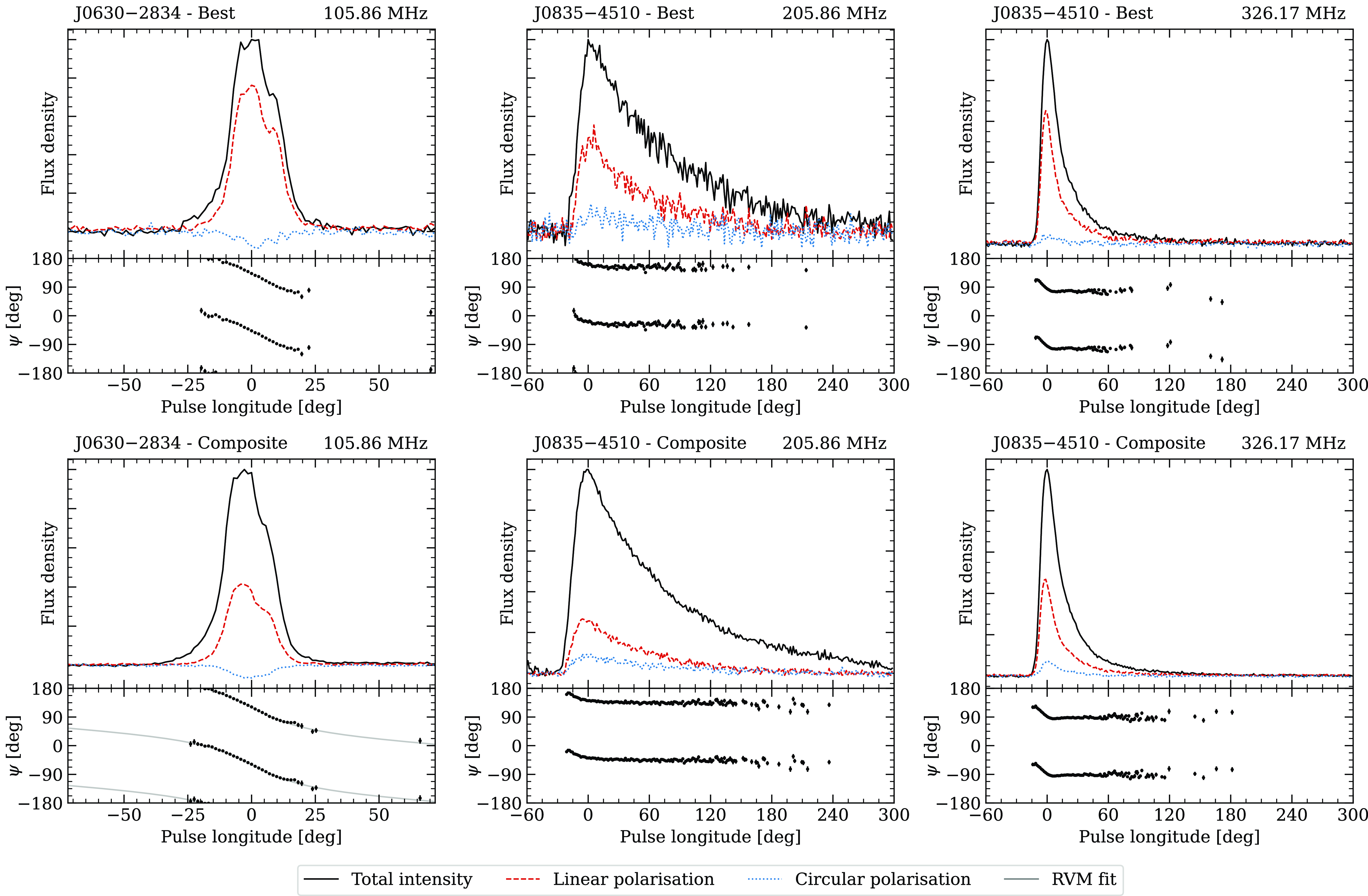
Full-Stokes integrated pulse profiles can provide useful insights into the accuracy and reproducibility of polarimetry. This is particularly important for the AAVS2, a prototype aperture array with novel technologies that are yet to be fully validated. In Fig. 2, we present polarimetric pulse profiles for both of the target pulsars. The top row shows the best detections for each frequency band, selected based on the linearly polarised signal-to-noise. The bottom row shows composite profiles created by phase-aligning and combining all of the integrated pulse profiles with uniform weights using psradd. The Faraday rotation was removed for each observation before the profiles were combined. For J0630
 $-$
2834, the best individual detection is consistent with detections from the Giant Metrewave Radio Telescope (GMRT) at 243 MHz (Johnston et al. Reference Johnston, Karastergiou, Mitra and Gupta2008) and the Murchison Widefield Array (MWA; Tingay et al. Reference Tingay2013; Wayth et al. Reference Wayth2018) between 140 and 200 MHz (Xue Reference Xue2019). At 326 MHz, the best individual profile of J0835
$-$
2834, the best individual detection is consistent with detections from the Giant Metrewave Radio Telescope (GMRT) at 243 MHz (Johnston et al. Reference Johnston, Karastergiou, Mitra and Gupta2008) and the Murchison Widefield Array (MWA; Tingay et al. Reference Tingay2013; Wayth et al. Reference Wayth2018) between 140 and 200 MHz (Xue Reference Xue2019). At 326 MHz, the best individual profile of J0835
 $-$
4510 is consistent with the detection from Hamilton et al. (1997) made using Murriyang (CSIRO’s Parkes 64-m radio telescope). At 206 MHz, the best AAVS2 detection is consistent with the full-Stokes profile from the MWA at the same frequency (Xue Reference Xue2019). The composite profiles display a significantly lower degree of polarisation than the individual observations. This is indicative of some residual error in the polarimetry, which will require further investigation to resolve.
$-$
4510 is consistent with the detection from Hamilton et al. (1997) made using Murriyang (CSIRO’s Parkes 64-m radio telescope). At 206 MHz, the best AAVS2 detection is consistent with the full-Stokes profile from the MWA at the same frequency (Xue Reference Xue2019). The composite profiles display a significantly lower degree of polarisation than the individual observations. This is indicative of some residual error in the polarimetry, which will require further investigation to resolve.
Full-Stokes integrated pulse profiles for J0630
 $-$
2834 at 105.86 MHz (left); and J0835
$-$
2834 at 105.86 MHz (left); and J0835
 $-$
4510 at 205.86 MHz (middle) and 326.17 MHz (right). All profiles are processed with 256 phase bins. The top row shows the best single observation based on the linearly polarised signal-to-noise ratio. The bottom row shows composite profiles of all observations in the given frequency band. For each subplot, the top panel shows the pulse profile in total intensity (Stokes I; black line), linear polarisation (Stokes
$-$
4510 at 205.86 MHz (middle) and 326.17 MHz (right). All profiles are processed with 256 phase bins. The top row shows the best single observation based on the linearly polarised signal-to-noise ratio. The bottom row shows composite profiles of all observations in the given frequency band. For each subplot, the top panel shows the pulse profile in total intensity (Stokes I; black line), linear polarisation (Stokes
 $\sqrt{Q^2+U^2}$
; red dashed line), and circular polarisation (Stokes V; blue dotted line). The lower panel shows the position angle for bins with
$\sqrt{Q^2+U^2}$
; red dashed line), and circular polarisation (Stokes V; blue dotted line). The lower panel shows the position angle for bins with
 $>3\sigma$
in linear polarisation. For the composite profile of J0630
$>3\sigma$
in linear polarisation. For the composite profile of J0630
 $-$
2834, the best-fit rotating vector model (RVM) is shown (grey line).
$-$
2834, the best-fit rotating vector model (RVM) is shown (grey line).
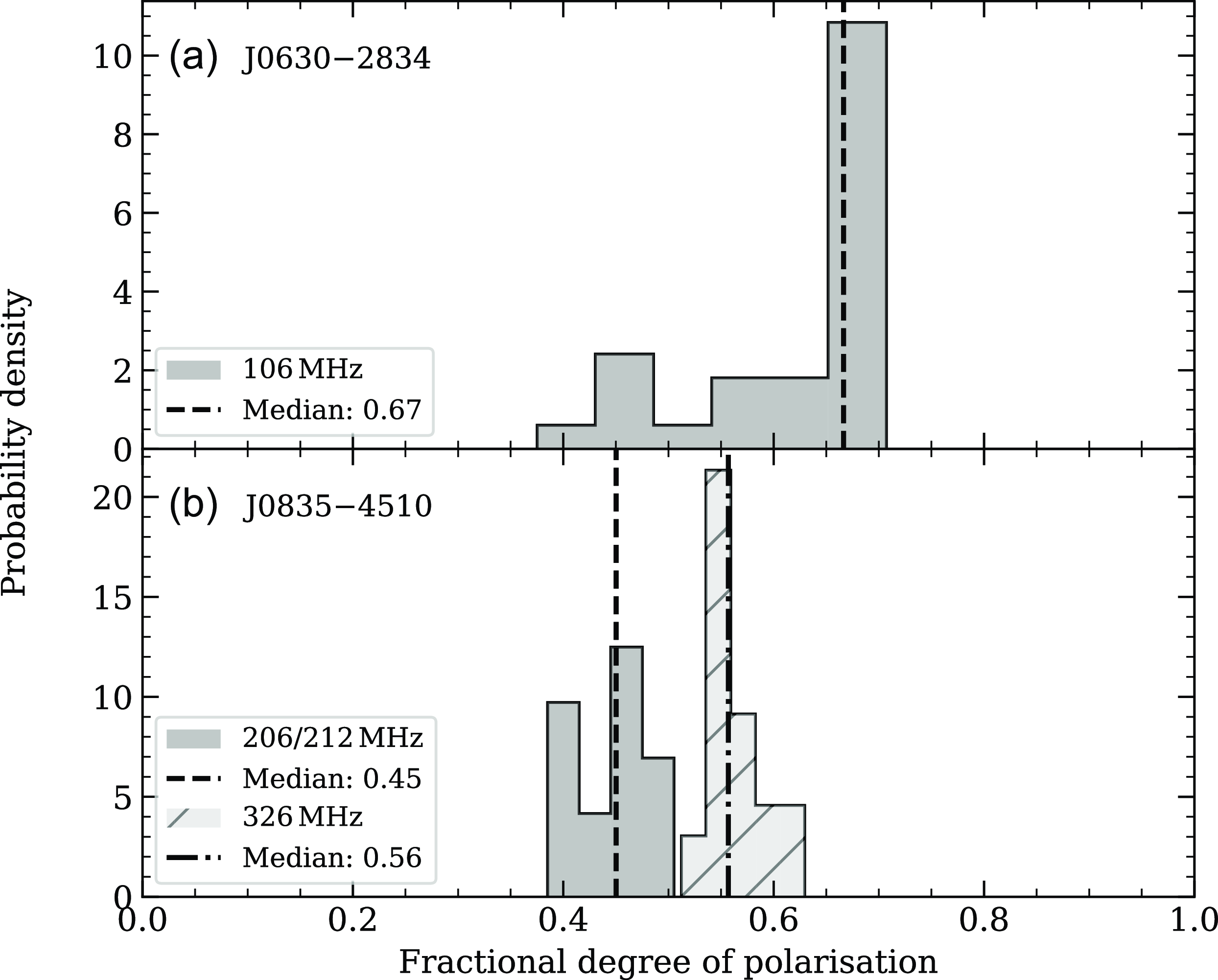
The degree of linear polarisation is expected to be intrinsically stable, which makes it possible to quantify the stability of the polarimetry between observations. For each profile, we measured the fractional degree of linear polarisation (p) and present the results in Fig. 3. For J0630
 $-$
2834, half of the observations have a fractional polarisation between 0.67 and 0.71, which is similar to what is reported by Johnston et al. (Reference Johnston, Karastergiou, Mitra and Gupta2008) and Xue (Reference Xue2019). However, the other half of the observations show a large spread of fractional polarisations, indicating some inconsistency in the quality of the uncalibrated polarimetry. We did not find any significant correlation between the fractional polarisation and the zenith angle, which suggests that the systematic depolarisation is not direction dependent. The fractional polarisations of J0835
$-$
2834, half of the observations have a fractional polarisation between 0.67 and 0.71, which is similar to what is reported by Johnston et al. (Reference Johnston, Karastergiou, Mitra and Gupta2008) and Xue (Reference Xue2019). However, the other half of the observations show a large spread of fractional polarisations, indicating some inconsistency in the quality of the uncalibrated polarimetry. We did not find any significant correlation between the fractional polarisation and the zenith angle, which suggests that the systematic depolarisation is not direction dependent. The fractional polarisations of J0835
 $-$
4510 are more consistent, with some variance that could be caused by the changing pulse broadening time between observing epochs (e.g. Xue Reference Xue2019). The range of fractional polarisations are consistent with measurements from Hamilton et al. (1997) and Xue (Reference Xue2019), with minor discrepancies which could be due to frequency-dependent depolarisation from stochastic fluctuations in the ISM (Burn Reference Burn1966).
$-$
4510 are more consistent, with some variance that could be caused by the changing pulse broadening time between observing epochs (e.g. Xue Reference Xue2019). The range of fractional polarisations are consistent with measurements from Hamilton et al. (1997) and Xue (Reference Xue2019), with minor discrepancies which could be due to frequency-dependent depolarisation from stochastic fluctuations in the ISM (Burn Reference Burn1966).
Histograms of the fractional degree of linear polarisation measured from AAVS2 detections. (a) Result for J0630
 $-$
2834 at 105.86 MHz. (b) Result for J0835
$-$
2834 at 105.86 MHz. (b) Result for J0835
 $-$
4510 at 205.86/212.11 MHz (dark grey) and 326.17 MHz (light grey, hatched). The median values are indicated by dashed and dot-dashed lines.
$-$
4510 at 205.86/212.11 MHz (dark grey) and 326.17 MHz (light grey, hatched). The median values are indicated by dashed and dot-dashed lines.
For J0630
 $-$
2834, we fit the rotating vector model (RVM; Radhakrishnan & Cooke Reference Radhakrishnan and Cooke1969) using PSRSALSA (Rookyard, Weltevrede, & Johnston Reference Rookyard, Weltevrede and Johnston2015; Weltevrede Reference Weltevrede2016). We used the routine ppolFit, which determines the allowed values of the magnetic inclination angle (
$-$
2834, we fit the rotating vector model (RVM; Radhakrishnan & Cooke Reference Radhakrishnan and Cooke1969) using PSRSALSA (Rookyard, Weltevrede, & Johnston Reference Rookyard, Weltevrede and Johnston2015; Weltevrede Reference Weltevrede2016). We used the routine ppolFit, which determines the allowed values of the magnetic inclination angle (
 $\alpha$
) and the impact parameter (
$\alpha$
) and the impact parameter (
 $\beta$
) by performing a grid search in the
$\beta$
) by performing a grid search in the
 $\alpha$
–
$\alpha$
–
 $\beta$
parameter space and measuring the reduced
$\beta$
parameter space and measuring the reduced
 $\chi^2$
for each trial. The 68% confidence interval of
$\chi^2$
for each trial. The 68% confidence interval of
 $\alpha$
and
$\alpha$
and
 $\beta$
was determined from the points at which the reduced
$\beta$
was determined from the points at which the reduced
 $\chi^2$
was equal to twice the global minimum. Using the AAVS2 composite profile at 105.86 MHz, we measure
$\chi^2$
was equal to twice the global minimum. Using the AAVS2 composite profile at 105.86 MHz, we measure
 $0\leq\alpha\leq 87.5\,\mathrm{deg}$
and
$0\leq\alpha\leq 87.5\,\mathrm{deg}$
and
 $-13.6\leq \beta\leq 0\,\mathrm{deg}$
. For comparison, we performed the same analysis on a pulse profile published by Johnston & Kerr (Reference Johnston and Kerr2018) at 1.4 GHz. In this case, we find
$-13.6\leq \beta\leq 0\,\mathrm{deg}$
. For comparison, we performed the same analysis on a pulse profile published by Johnston & Kerr (Reference Johnston and Kerr2018) at 1.4 GHz. In this case, we find
 $0\leq\alpha\leq 92.8\,\mathrm{deg}$
and
$0\leq\alpha\leq 92.8\,\mathrm{deg}$
and
 $-14.1\leq \beta\leq 0\,\mathrm{deg}$
. The AAVS2 measurements are therefore consistent with Johnston & Kerr (Reference Johnston and Kerr2018), and place marginally stronger constraints on
$-14.1\leq \beta\leq 0\,\mathrm{deg}$
. The AAVS2 measurements are therefore consistent with Johnston & Kerr (Reference Johnston and Kerr2018), and place marginally stronger constraints on
 $\alpha$
and
$\alpha$
and
 $\beta$
. In the lower left subplot of Fig. 2, we show the RVM fit with the minimum reduced
$\beta$
. In the lower left subplot of Fig. 2, we show the RVM fit with the minimum reduced
 $\chi^2$
; that is,
$\chi^2$
; that is,
 $\alpha=0.52\,\mathrm{deg}$
and
$\alpha=0.52\,\mathrm{deg}$
and
 $\beta=-0.12\,\mathrm{deg}$
.
$\beta=-0.12\,\mathrm{deg}$
.
4.2. Validation of ionospheric models
Due to the large fractional bandwidth, the AAVS2 is capable of determining pulsar RMs with exceptional precision. For our observations of J0630
 $-$
2834 centred at 106 MHz, 95% of the RM uncertainties are between
$-$
2834 centred at 106 MHz, 95% of the RM uncertainties are between
 $\sim$
0.01–0.04
$\sim$
0.01–0.04
 $\mathrm{rad}\,\mathrm{m}^{-2}$
. For comparison, the 95% confidence lower bound of the distribution of RM uncertainties reported in the ATNF pulsar catalogue (v1.71) is
$\mathrm{rad}\,\mathrm{m}^{-2}$
. For comparison, the 95% confidence lower bound of the distribution of RM uncertainties reported in the ATNF pulsar catalogue (v1.71) is
 $\sim$
0.06
$\sim$
0.06
 $\mathrm{rad}\,\mathrm{m}^{-2}$
(Manchester et al. Reference Manchester, Hobbs, Teoh and Hobbs2005). It is therefore clear that the AAVS2 can determine RM to a precision significantly better than telescopes operating at higher frequencies. This feature makes the AAVS2 well suited for monitoring small variations in ionospheric RM on short timescales (
$\mathrm{rad}\,\mathrm{m}^{-2}$
(Manchester et al. Reference Manchester, Hobbs, Teoh and Hobbs2005). It is therefore clear that the AAVS2 can determine RM to a precision significantly better than telescopes operating at higher frequencies. This feature makes the AAVS2 well suited for monitoring small variations in ionospheric RM on short timescales (
 $\sim$
hours), which is useful for testing the accuracy of ionospheric models.
$\sim$
hours), which is useful for testing the accuracy of ionospheric models.
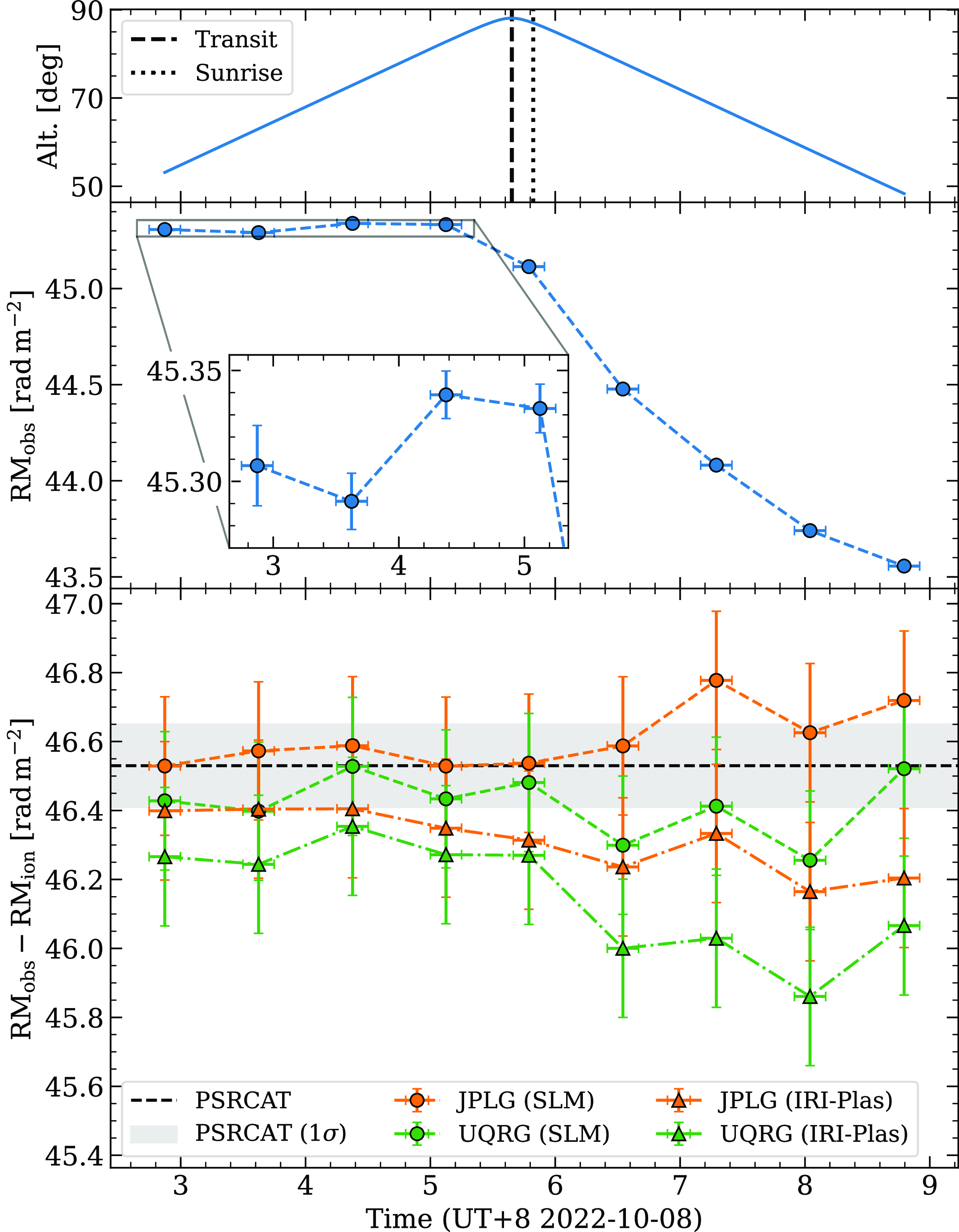
In Fig. 4, we present the observed and ionosphere-subtracted RMs for nine observations of J0630
 $-$
2834 over a
$-$
2834 over a
 $\sim$
6 h time period on UT+8 2022-10-08. The first four observations were collected before local sunrise and show small variations of the order
$\sim$
6 h time period on UT+8 2022-10-08. The first four observations were collected before local sunrise and show small variations of the order
 $\sim$
0.01
$\sim$
0.01
 $\mathrm{rad}\,\mathrm{m}^{-2}$
(see the inset in Fig. 4). After sunrise, we observe the expected downward trend in
$\mathrm{rad}\,\mathrm{m}^{-2}$
(see the inset in Fig. 4). After sunrise, we observe the expected downward trend in
 $\mathrm{RM}_\mathrm{obs}$
due to the diurnal photoionisation of the ionosphere. The diurnal trend is the largest source of potential error in the estimated RM of the ISM. Therefore, it is essential that this modulation is properly subtracted. As a simple test, we compare the residual RMs after subtracting the estimated
$\mathrm{RM}_\mathrm{obs}$
due to the diurnal photoionisation of the ionosphere. The diurnal trend is the largest source of potential error in the estimated RM of the ISM. Therefore, it is essential that this modulation is properly subtracted. As a simple test, we compare the residual RMs after subtracting the estimated
 $\mathrm{RM}_\mathrm{ion}$
from two GIMs (JPLG and UQRG) with and without scaling using the IRI-Plas ionospheric density profile (see Fig. 4, bottom panel). For reference, we also show the most up to date RM in the ATNF pulsar catalogue (from Johnston et al. Reference Johnston, Hobbs, Vigeland and Kramer2005).
$\mathrm{RM}_\mathrm{ion}$
from two GIMs (JPLG and UQRG) with and without scaling using the IRI-Plas ionospheric density profile (see Fig. 4, bottom panel). For reference, we also show the most up to date RM in the ATNF pulsar catalogue (from Johnston et al. Reference Johnston, Hobbs, Vigeland and Kramer2005).
Temporal RM variations towards J0630
 $-$
2834 over a
$-$
2834 over a
 $\sim$
6 h period on UT+8 2022-10-08. The top plot shows the source altitude over time, transiting just before sunrise (the time when the Sun reaches an altitude of 0 deg). The middle plot shows the observed RM; the inset shows the small RM variations detected before sunrise. The bottom plot shows the ionosphere-subtracted RMs for JPLG (orange) and UQRG (green) TEC maps with the single-layer model (SLM; circles) and the plasmasphere-extended SLM (IRI-Plas; triangles). For reference, we include the RM reported in the ATNF pulsar catalogue from Johnston et al. (Reference Johnston, Hobbs, Vigeland and Kramer2005) (black dashed line) and the corresponding uncertainty estimate (grey shaded region).
$\sim$
6 h period on UT+8 2022-10-08. The top plot shows the source altitude over time, transiting just before sunrise (the time when the Sun reaches an altitude of 0 deg). The middle plot shows the observed RM; the inset shows the small RM variations detected before sunrise. The bottom plot shows the ionosphere-subtracted RMs for JPLG (orange) and UQRG (green) TEC maps with the single-layer model (SLM; circles) and the plasmasphere-extended SLM (IRI-Plas; triangles). For reference, we include the RM reported in the ATNF pulsar catalogue from Johnston et al. (Reference Johnston, Hobbs, Vigeland and Kramer2005) (black dashed line) and the corresponding uncertainty estimate (grey shaded region).
Since the ISM does not vary appreciably on the timescale of hours, we expect any temporal variations in
 $\mathrm{RM}_\mathrm{obs}-\mathrm{RM}_\mathrm{ion}$
(the ‘residual’ RM) on this timescale to be due to the imperfect subtraction of ionospheric variability. Additionally, because J0630
$\mathrm{RM}_\mathrm{obs}-\mathrm{RM}_\mathrm{ion}$
(the ‘residual’ RM) on this timescale to be due to the imperfect subtraction of ionospheric variability. Additionally, because J0630
 $-$
2834 lies outside of the Gum Nebula, it is not expected show any long-term change in RM. Variations in the residual RM on longer timescales could therefore also be due to the ionospheric model. To quantify these variations, we use the mean absolute deviationFootnote d from the mean of the data. We find that the RM residuals from the single-layer model deviate less than the estimates made using the plasmasphere-extended model (i.e. the single-layer model scaled by the IRI-Plas density profile). Furthermore, we see greater deviations during the daytime hours, especially for the plasmasphere-extended model (see Fig. 4). The trend suggests that the plasmasphere-extended model overestimates the ionospheric contribution. Between the two GIMs, we find that JPLG deviates less overall than UQRG, which is due to several significant outliers in the UQRG estimates. The outliers from the UQRG GIM may be a result of the poor GNSS receiver coverage at the MRO, which we discuss further in Section 5.2. Interestingly, UQRG shows a lower deviation than JPLG when the outliers are excluded. Nevertheless, we use JPLG for all further analysis as it appears to yield more consistent results.
$-$
2834 lies outside of the Gum Nebula, it is not expected show any long-term change in RM. Variations in the residual RM on longer timescales could therefore also be due to the ionospheric model. To quantify these variations, we use the mean absolute deviationFootnote d from the mean of the data. We find that the RM residuals from the single-layer model deviate less than the estimates made using the plasmasphere-extended model (i.e. the single-layer model scaled by the IRI-Plas density profile). Furthermore, we see greater deviations during the daytime hours, especially for the plasmasphere-extended model (see Fig. 4). The trend suggests that the plasmasphere-extended model overestimates the ionospheric contribution. Between the two GIMs, we find that JPLG deviates less overall than UQRG, which is due to several significant outliers in the UQRG estimates. The outliers from the UQRG GIM may be a result of the poor GNSS receiver coverage at the MRO, which we discuss further in Section 5.2. Interestingly, UQRG shows a lower deviation than JPLG when the outliers are excluded. Nevertheless, we use JPLG for all further analysis as it appears to yield more consistent results.
4.3. Temporal RM variations
In Fig. 5, we show the complete RM time series for each pulsar before and after subtracting the JPLG/SLM model. To determine the best estimate of
 $\mathrm{RM}_\mathrm{ISM}$
, we measure the weighted mean of
$\mathrm{RM}_\mathrm{ISM}$
, we measure the weighted mean of
 $\mathrm{RM}_\mathrm{obs}-\mathrm{RM}_\mathrm{ion}$
by fitting a constant (time-independent) model with a Gaussian likelihood. We set a uniform prior probability and used the Bayesian inference library Bilby to estimate the posterior probability distribution (Ashton et al. Reference Ashton2019). The median and 1, 2, and 3
$\mathrm{RM}_\mathrm{obs}-\mathrm{RM}_\mathrm{ion}$
by fitting a constant (time-independent) model with a Gaussian likelihood. We set a uniform prior probability and used the Bayesian inference library Bilby to estimate the posterior probability distribution (Ashton et al. Reference Ashton2019). The median and 1, 2, and 3
 $\sigma$
credible intervals of the model fit are shown in Fig. 5.
$\sigma$
credible intervals of the model fit are shown in Fig. 5.
RM time series for J0630
 $-$
2834 (left) and J0835
$-$
2834 (left) and J0835
 $-$
4510 (right). Each plot shows the RM before (blue circles) and after (orange diamonds) subtracting the ionospheric RM. We show the weighted mean (black line) of the ionosphere-corrected RM, and the 1, 2, and 3
$-$
4510 (right). Each plot shows the RM before (blue circles) and after (orange diamonds) subtracting the ionospheric RM. We show the weighted mean (black line) of the ionosphere-corrected RM, and the 1, 2, and 3
 $\sigma$
credible intervals of the posterior probability distribution (grey shaded bands).
$\sigma$
credible intervals of the posterior probability distribution (grey shaded bands).
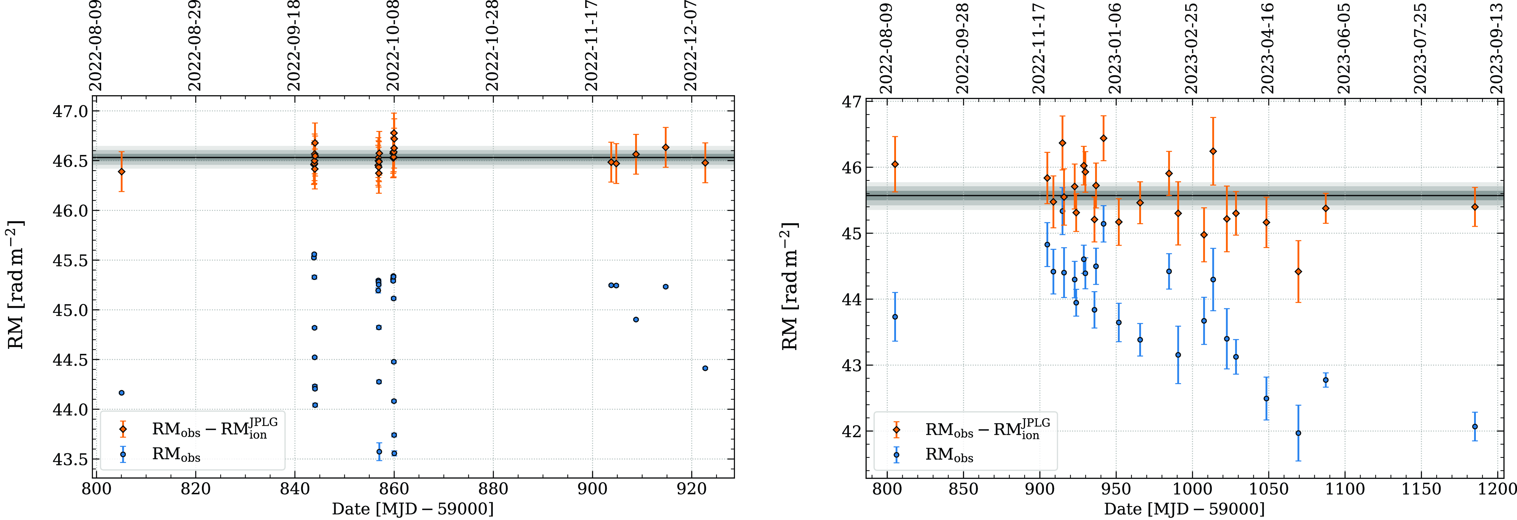
For J0630
 $-$
2834, we measure a weighted mean of
$-$
2834, we measure a weighted mean of
 $46.53\pm 0.04$
 $\mathrm{rad}\,\mathrm{m}^{-2}$
(where the uncertainty is the 1
$\mathrm{rad}\,\mathrm{m}^{-2}$
(where the uncertainty is the 1
 $\sigma$
credible interval), which is in excellent agreement with the value of
$\sigma$
credible interval), which is in excellent agreement with the value of
 $46.53\pm0.12$
 $\mathrm{rad}\,\mathrm{m}^{-2}$
from Johnston et al. (Reference Johnston, Hobbs, Vigeland and Kramer2005). The RM uncertainties all overlap with the weighted mean of the data, which is indicative that the uncertainties may be overestimated. However, the conservatively large uncertainties account for the lack of knowledge about the accuracy of ionospheric models at the MRO. A linear model fit to the data shows that the gradient is consistent with zero to within 1
$\mathrm{rad}\,\mathrm{m}^{-2}$
from Johnston et al. (Reference Johnston, Hobbs, Vigeland and Kramer2005). The RM uncertainties all overlap with the weighted mean of the data, which is indicative that the uncertainties may be overestimated. However, the conservatively large uncertainties account for the lack of knowledge about the accuracy of ionospheric models at the MRO. A linear model fit to the data shows that the gradient is consistent with zero to within 1
 $\sigma$
.
$\sigma$
.
For J0835
 $-$
4510, the observed RM decreases over time due to the shift in transit time (and thus the observing time) throughout the year. After subtracting the JPLG/SLM model, we measure a weighted mean RM of
$-$
4510, the observed RM decreases over time due to the shift in transit time (and thus the observing time) throughout the year. After subtracting the JPLG/SLM model, we measure a weighted mean RM of
 $45.57\pm 0.07$
 $\mathrm{rad}\,\mathrm{m}^{-2}$
, which is consistent with the value of
$\mathrm{rad}\,\mathrm{m}^{-2}$
, which is consistent with the value of
 $45.3\pm 0.7$
 $\mathrm{rad}\,\mathrm{m}^{-2}$
from Sobey et al. (Reference Sobey2021). We also observe a residual gradient of
$\mathrm{rad}\,\mathrm{m}^{-2}$
from Sobey et al. (Reference Sobey2021). We also observe a residual gradient of
 $-0.8\pm0.3$
 $\mathrm{rad}\,\mathrm{m}^{-2}\,\mathrm{yr}^{-1}$
, which could be the result of a systematic error in the ionospheric model. For example, Porayko et al. (Reference Porayko2019) observed a systematic error with a period of 1 d in RM residuals after subtracting the JPLG model. This could cause a corresponding error with a period of 1 yr in our data, due to the observations being collected at progressively earlier times of day. An error of this kind would be less significant in the RM series of J0630
$\mathrm{rad}\,\mathrm{m}^{-2}\,\mathrm{yr}^{-1}$
, which could be the result of a systematic error in the ionospheric model. For example, Porayko et al. (Reference Porayko2019) observed a systematic error with a period of 1 d in RM residuals after subtracting the JPLG model. This could cause a corresponding error with a period of 1 yr in our data, due to the observations being collected at progressively earlier times of day. An error of this kind would be less significant in the RM series of J0630
 $-$
2834, which spans only
$-$
2834, which spans only
 $\sim$
0.3 yr compared to
$\sim$
0.3 yr compared to
 $\sim$
1 yr for Vela and has sparser temporal coverage. If instead we subtract the UQRG/SLM model, we find that the gradient is consistent with zero. The fact that the long-term trend is model dependent is evidence that the trend is systematic in origin, caused by inaccuracies in the JPLG model on an annual timescale. Observations over multiple years will be required to disentangle model systematics from the underlying astrophysical trend.
$\sim$
1 yr for Vela and has sparser temporal coverage. If instead we subtract the UQRG/SLM model, we find that the gradient is consistent with zero. The fact that the long-term trend is model dependent is evidence that the trend is systematic in origin, caused by inaccuracies in the JPLG model on an annual timescale. Observations over multiple years will be required to disentangle model systematics from the underlying astrophysical trend.
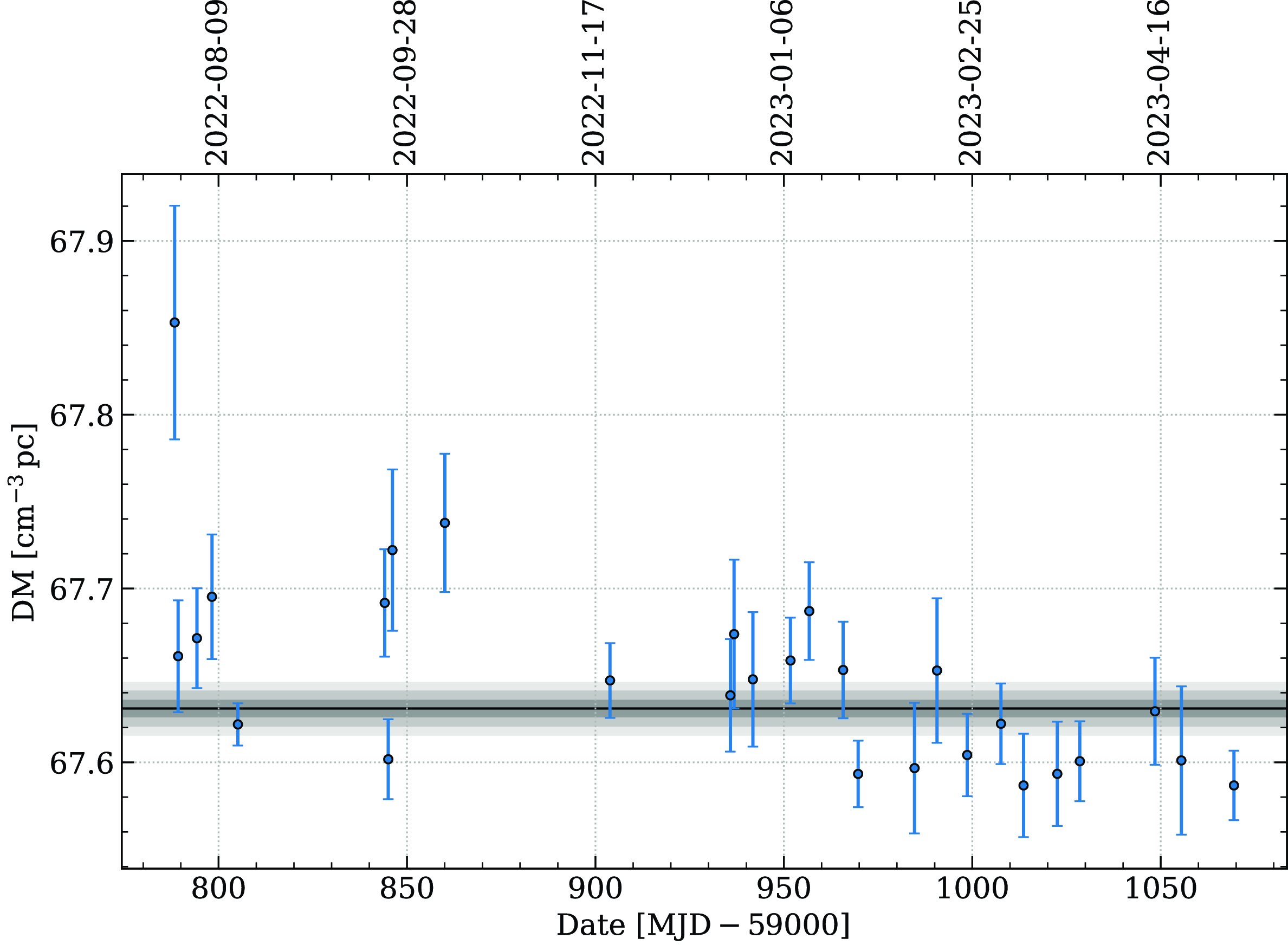
4.4. Temporal DM variations
In Fig. 6, we show the measured DMs for J0835
 $-$
4510 from observations at 326.17 MHz. As in Section 4.3, we fit a constant model with a Gaussian likelihood and measure a weighted mean value of
$-$
4510 from observations at 326.17 MHz. As in Section 4.3, we fit a constant model with a Gaussian likelihood and measure a weighted mean value of
 $67.63\pm 0.01$
 $\mathrm{cm}^{-3}\,\mathrm{pc}$
. The time series shows outliers and correlated variability that could be attributed to temporal variations in the pulse broadening time. Such variations can bias the pulse arrival times due to discrepancies between the template profile and the individual observations. A detailed analysis of these variations, including the influence of scattering on the DM measurements, is beyond the scope of this work, and will be deferred to a future publication.
$\mathrm{cm}^{-3}\,\mathrm{pc}$
. The time series shows outliers and correlated variability that could be attributed to temporal variations in the pulse broadening time. Such variations can bias the pulse arrival times due to discrepancies between the template profile and the individual observations. A detailed analysis of these variations, including the influence of scattering on the DM measurements, is beyond the scope of this work, and will be deferred to a future publication.
DM time series for J0835
 $-$
4510. We show the weighted mean (black line) and the 1, 2, and 3
$-$
4510. We show the weighted mean (black line) and the 1, 2, and 3
 $\sigma$
credible intervals of the posterior probability distribution (grey shaded bands).
$\sigma$
credible intervals of the posterior probability distribution (grey shaded bands).
5. Discussion
5.1. Long-term RM and DM variations
The RM and DM of the Vela pulsar have long been observed to change significantly over time, initially showing a correlated linear trend which was attributed to the relative movement of the pulsar and a compact overdensity (filament) of magnetised plasma within the Vela SNR (Hamilton et al. Reference Hamilton, McCulloch, Ables and Komesaroff1977). Later analysis of RM measurements published over several decades revealed a more complex deterministic trend; Xue (Reference Xue2019) suggest that the variations in RM could be explained by an inhomogeneous magnetic field within the plasma filament.
In this section, we focus on the most recent two decades of RM and DM variations for the Vela pulsar, which is yet to be analysed in detail in the literature. In Fig. 7, we plot all published RM and DM measurements since 2006, including the measurements from this work. From visual inspection of the data, it is immediately apparent that the DM decreased by
 $\sim$
0.3–0.4
$\sim$
0.3–0.4
 $\mathrm{cm}^{-3}\,\mathrm{pc}$
between MJD
$\mathrm{cm}^{-3}\,\mathrm{pc}$
between MJD
 $\sim$
56 000 (Petroff et al. Reference Petroff, Keith, Johnston, van Straten and Shannon2013) and MJD
$\sim$
56 000 (Petroff et al. Reference Petroff, Keith, Johnston, van Straten and Shannon2013) and MJD
 $\sim$
60 000 (this work). The sparsity of published data between these dates makes it difficult to disentangle the true change in astrophysical DM with systematic differences due to the profile evolution with frequency and measurement methods. However, the agreement in DM between Murriyang observations at
$\sim$
60 000 (this work). The sparsity of published data between these dates makes it difficult to disentangle the true change in astrophysical DM with systematic differences due to the profile evolution with frequency and measurement methods. However, the agreement in DM between Murriyang observations at
 $\sim$
700–4 000 MHz (Sobey et al. Reference Sobey2021) and MWA observations at
$\sim$
700–4 000 MHz (Sobey et al. Reference Sobey2021) and MWA observations at
 $\sim$
170–230 MHz (Xue Reference Xue2019) collected on similar observing epochs (MJD
$\sim$
170–230 MHz (Xue Reference Xue2019) collected on similar observing epochs (MJD
 $\sim$
58 400–58 900) suggests that the systematic offset arising from the difference in observing frequencies may not be significant to first order. With this in mind, the recent decrease in DM suggests that, contrary to the conclusions of Petroff et al. (Reference Petroff, Keith, Johnston, van Straten and Shannon2013), the filament seen by Hamilton et al. (Reference Hamilton, McCulloch, Ables and Komesaroff1977) may still be moving out of the line of sight.
$\sim$
58 400–58 900) suggests that the systematic offset arising from the difference in observing frequencies may not be significant to first order. With this in mind, the recent decrease in DM suggests that, contrary to the conclusions of Petroff et al. (Reference Petroff, Keith, Johnston, van Straten and Shannon2013), the filament seen by Hamilton et al. (Reference Hamilton, McCulloch, Ables and Komesaroff1977) may still be moving out of the line of sight.
Published measurements of RM (top) and DM (bottom) for J0835
 $-$
4510 between 2006 and 2023. The black dashed lines show the median simple linear models and the black dot-dashed lines show the median piecewise linear models. The thin orange and blue lines show 100 random samples from the posterior distributions of the simple and piecewise model fits, respectively. The diamond markers show measurements obtained using the AAVS2 in this work; the circle markers show data from Noutsos et al. (Reference Noutsos, Johnston, Kramer and Karastergiou2008), Petroff et al. (Reference Petroff, Keith, Johnston, van Straten and Shannon2013), Lenc et al. (Reference Lenc2017), Han et al. (Reference Han, Manchester and van Straten2018), Xue (Reference Xue2019), Sobey et al. (Reference Sobey2021), Posselt et al. (Reference Posselt2023). We show horizontal error bars for Sobey et al. (Reference Sobey2021) as the measurements are averaged over multiple observations (the horizontal uncertainties were not included in the model fits).
$-$
4510 between 2006 and 2023. The black dashed lines show the median simple linear models and the black dot-dashed lines show the median piecewise linear models. The thin orange and blue lines show 100 random samples from the posterior distributions of the simple and piecewise model fits, respectively. The diamond markers show measurements obtained using the AAVS2 in this work; the circle markers show data from Noutsos et al. (Reference Noutsos, Johnston, Kramer and Karastergiou2008), Petroff et al. (Reference Petroff, Keith, Johnston, van Straten and Shannon2013), Lenc et al. (Reference Lenc2017), Han et al. (Reference Han, Manchester and van Straten2018), Xue (Reference Xue2019), Sobey et al. (Reference Sobey2021), Posselt et al. (Reference Posselt2023). We show horizontal error bars for Sobey et al. (Reference Sobey2021) as the measurements are averaged over multiple observations (the horizontal uncertainties were not included in the model fits).
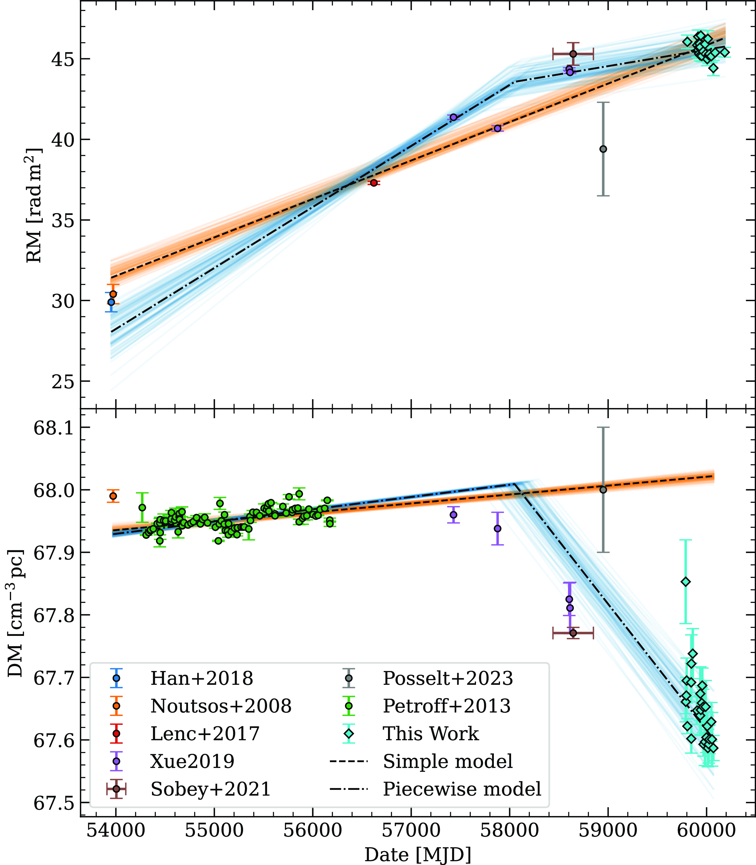
Following previous analysis in the literature (e.g. Hamilton et al. Reference Hamilton, McCulloch, Ables and Komesaroff1977; Petroff et al. Reference Petroff, Keith, Johnston, van Straten and Shannon2013; Xue Reference Xue2019) we fit linear models to measure the gradients in DM and RM over time. Specifically, we consider a simple (one-segment) and a piecewise (two-segment) linear model. Since the RM and DM both depend on the thermal electron density along the line of sight, a significant change in density could result in a correlated change in both quantities. To account for this, we have enforced that the break point in the piecewise model is the same for both the RM and DM. We jointly fit the RM and DM data using a Gaussian likelihood and make use of the Huber loss function to reduce the weighting of outliers greater than 1.345
 $\sigma$
from the model (see Appendix 1 for further details about the model fitting procedure). This approach results in a model fit which is less constrained by measurements with underestimated uncertainties or large systematic offsets from the rest of the data.
$\sigma$
from the model (see Appendix 1 for further details about the model fitting procedure). This approach results in a model fit which is less constrained by measurements with underestimated uncertainties or large systematic offsets from the rest of the data.
In Table 2, we present estimates of the RM and DM gradients and the magnetic field strength computed using equation (2). We estimate each parameter using the median of the posterior distribution, with the uncertainties indicating the 68% credible interval. From the simple linear model fit, we measure
 $\langle B_\parallel\rangle_\mathrm{var} = 206^{+23}_{-19}\,\mu\mathrm{G}$
. The piecewise model fit deviates significantly from the simple model, suggesting that the mean magnetic field in the time-varying region transitions from
$\langle B_\parallel\rangle_\mathrm{var} = 206^{+23}_{-19}\,\mu\mathrm{G}$
. The piecewise model fit deviates significantly from the simple model, suggesting that the mean magnetic field in the time-varying region transitions from
 $240^{+30}_{-20}\,\mu\mathrm{G}$
to
$240^{+30}_{-20}\,\mu\mathrm{G}$
to
 $-6.2^{+0.7}_{-0.9}\,\mu\mathrm{G}$
at around MJD
$-6.2^{+0.7}_{-0.9}\,\mu\mathrm{G}$
at around MJD
 $58\,050^{+90}_{-100}$
. The Bayes factor (i.e. the difference in evidence) between the two model fits is
$58\,050^{+90}_{-100}$
. The Bayes factor (i.e. the difference in evidence) between the two model fits is
 $\log\mathcal{B}=535.9\pm 0.2$
, which strongly favours the piecewise model. The sign change implies that the mean direction of the magnetic field changes from pointing towards the observer to pointing towards the pulsar. Whilst the estimated magnetic field strengths exceed previous estimates for the Vela pulsar (
$\log\mathcal{B}=535.9\pm 0.2$
, which strongly favours the piecewise model. The sign change implies that the mean direction of the magnetic field changes from pointing towards the observer to pointing towards the pulsar. Whilst the estimated magnetic field strengths exceed previous estimates for the Vela pulsar (
 $\sim$
20--90
$\sim$
20--90
 $\mu\mathrm{G}$
; Hamilton, Hall, & Costa Reference Hamilton, Hall and Costa1985; Xue Reference Xue2019), they are not unreasonable for SNRs. For example, Rankin et al. (Reference Rankin, Campbell, Isaacman and Payne1988) measured
$\mu\mathrm{G}$
; Hamilton, Hall, & Costa Reference Hamilton, Hall and Costa1985; Xue Reference Xue2019), they are not unreasonable for SNRs. For example, Rankin et al. (Reference Rankin, Campbell, Isaacman and Payne1988) measured
 $\langle B_\parallel\rangle_\mathrm{var}=170\,\mu\mathrm{G}$
for the Crab pulsar.
$\langle B_\parallel\rangle_\mathrm{var}=170\,\mu\mathrm{G}$
for the Crab pulsar.
Estimated RM and DM gradients and the implied mean magnetic field strength of the magnetised plasma filament. The first row shows the results from a simple linear model; the second and third rows show the results from a piecewise linear model with a variable break point. The columns (from left to right) are: the start and end dates of the linear segment; the transverse scale size probed by the linear model (
 $\ell$
); the RM gradient (
$\ell$
); the RM gradient (
 $\mathrm{dRM}/\mathrm{d}t$
); the DM gradient (
$\mathrm{dRM}/\mathrm{d}t$
); the DM gradient (
 $\mathrm{dDM}/\mathrm{d}t$
); the mean magnetic field of the time-varying region parallel to the line of sight (
$\mathrm{dDM}/\mathrm{d}t$
); the mean magnetic field of the time-varying region parallel to the line of sight (
 $\langle B_\parallel \rangle_\mathrm{var}$
); and the change in electron density (
$\langle B_\parallel \rangle_\mathrm{var}$
); and the change in electron density (
 $\Delta n_e$
). See text for details.
$\Delta n_e$
). See text for details.
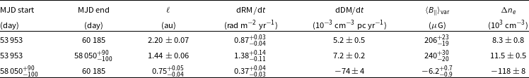
Following Hamilton et al. (Reference Hamilton, McCulloch, Ables and Komesaroff1977), we can estimate the transverse scale length of the pulsar’s path through the ISM as
 $\ell = v_\perp \Delta t$
, where
$\ell = v_\perp \Delta t$
, where
 $v_\perp$
is the transverse space velocity in
$v_\perp$
is the transverse space velocity in
 $\mathrm{pc}\,\mathrm{yr}^{-1}$
and
$\mathrm{pc}\,\mathrm{yr}^{-1}$
and
 $\Delta t$
is the time span in years. Assuming a similar scale in the line-of-sight dimension, the excess electron density in the time-varying region (i.e. the change in electron density) is
$\Delta t$
is the time span in years. Assuming a similar scale in the line-of-sight dimension, the excess electron density in the time-varying region (i.e. the change in electron density) is
 $\Delta n_e = (\mathrm{dDM}/\mathrm{d}t) v_\perp^{-1}$
. The Vela pulsar has a measured transverse velocity of
$\Delta n_e = (\mathrm{dDM}/\mathrm{d}t) v_\perp^{-1}$
. The Vela pulsar has a measured transverse velocity of
 $61\pm 2\,\mathrm{km}\,\mathrm{s}^{-1}$
(Dodson et al. Reference Dodson, Legge, Reynolds and McCulloch2003), or equivalently,
$61\pm 2\,\mathrm{km}\,\mathrm{s}^{-1}$
(Dodson et al. Reference Dodson, Legge, Reynolds and McCulloch2003), or equivalently,
 $(6.2\pm0.2) \times 10^{-7}\,\mathrm{pc}\,\mathrm{yr}^{-1}$
, placing it at the low end of the velocity distribution for young pulsars (e.g. Lyne & Lorimer Reference Lyne and Lorimer1994). The derived measurements are included in Table 2. We find that the scale lengths of the time-varying regions in the model fits are around
$(6.2\pm0.2) \times 10^{-7}\,\mathrm{pc}\,\mathrm{yr}^{-1}$
, placing it at the low end of the velocity distribution for young pulsars (e.g. Lyne & Lorimer Reference Lyne and Lorimer1994). The derived measurements are included in Table 2. We find that the scale lengths of the time-varying regions in the model fits are around
 $\sim$
1–2 au. From the simple model fit, we measure an increase in density of
$\sim$
1–2 au. From the simple model fit, we measure an increase in density of
 $(8.3\pm 0.8)\times 10^3\,\mathrm{cm}^{-3}$
. The piecewise model shows a similar density increase before the break point, followed by a steep decrease of
$(8.3\pm 0.8)\times 10^3\,\mathrm{cm}^{-3}$
. The piecewise model shows a similar density increase before the break point, followed by a steep decrease of
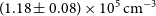 $(1.18\pm 0.08)\times 10^5\,\mathrm{cm}^{-3}$
after the break point. These density measurements are at least 1–2 orders of magnitude greater than some estimates for bright filaments in the Crab nebula (Osterbrock Reference Osterbrock1957; Woltjer Reference Woltjer1958). Interestingly, the observed structure is comparable in density and length scale with discrete compact structures associated with extreme scattering events in the ISM (e.g. Fiedler et al. Reference Fiedler, Dennison, Johnston and Hewish1987; Clegg, Fey, & Lazio Reference Clegg, Fey and Lazio1998; Dong, Petropoulou, & Giannios Reference Dong, Petropoulou and Giannios2018), which may reside in old supernova remnants (Romani, Blandford, & Cordes Reference Romani, Blandford and Cordes1987). Of course, another way to reconcile the high implied densities is to consider a structure which is significantly elongated along the line of sight, in which case our measurements would be overestimated. In any case, further observations will be required to better understand the origin of the structure.
$(1.18\pm 0.08)\times 10^5\,\mathrm{cm}^{-3}$
after the break point. These density measurements are at least 1–2 orders of magnitude greater than some estimates for bright filaments in the Crab nebula (Osterbrock Reference Osterbrock1957; Woltjer Reference Woltjer1958). Interestingly, the observed structure is comparable in density and length scale with discrete compact structures associated with extreme scattering events in the ISM (e.g. Fiedler et al. Reference Fiedler, Dennison, Johnston and Hewish1987; Clegg, Fey, & Lazio Reference Clegg, Fey and Lazio1998; Dong, Petropoulou, & Giannios Reference Dong, Petropoulou and Giannios2018), which may reside in old supernova remnants (Romani, Blandford, & Cordes Reference Romani, Blandford and Cordes1987). Of course, another way to reconcile the high implied densities is to consider a structure which is significantly elongated along the line of sight, in which case our measurements would be overestimated. In any case, further observations will be required to better understand the origin of the structure.
One potential cause for a large magnetic field gradient is a compression due to shocks in the ISM. Assuming a simple spherical compression, the magnetic field strength and electron density are positively correlated such that
 $B\propto n_e^{2/3}$
(e.g. Seta & Federrath Reference Seta and Federrath2022). In this case, the decrease in magnetic field strength derived from the piecewise model fit corresponds to a density decrease by a factor of
$B\propto n_e^{2/3}$
(e.g. Seta & Federrath Reference Seta and Federrath2022). In this case, the decrease in magnetic field strength derived from the piecewise model fit corresponds to a density decrease by a factor of
 $\sim$
240. For a decrease in density of
$\sim$
240. For a decrease in density of
 $10^5\,\mathrm{cm}^{-3}$
, the final density in the time-varying region is
$10^5\,\mathrm{cm}^{-3}$
, the final density in the time-varying region is
 $\sim$
 $420\,\mathrm{cm}^{-3}$
. It is important to note that the power-law relation is an idealised model and the true relation is more complex in a turbulent medium (Seta & Federrath Reference Seta and Federrath2022).
$420\,\mathrm{cm}^{-3}$
. It is important to note that the power-law relation is an idealised model and the true relation is more complex in a turbulent medium (Seta & Federrath Reference Seta and Federrath2022).
In the above analysis, we have assumed that the time-varying region is a single compact structure. It is also possible that the observed variations are the result of multiple structures at different locations along the line of sight. In principle, this could be tested by observing interstellar scintillation in Vela pulsar observations at higher frequencies, which can be used to determine the location of one or multiple scattering screens (e.g. Reardon et al. Reference Reardon2020). Alternatively, this could be tested via accurate modelling of the pulse shapes at low observing frequencies (
 $\lesssim$
300 MHz), which may necessitate reliably disentangling the profile evolution (in frequency) and frequency-dependent effects of pulse broadening that arise from multipath scattering (e.g. Bhat et al. Reference Bhat, Cordes, Camilo, Nice and Lorimer2004; Geyer et al. Reference Geyer2017).
$\lesssim$
300 MHz), which may necessitate reliably disentangling the profile evolution (in frequency) and frequency-dependent effects of pulse broadening that arise from multipath scattering (e.g. Bhat et al. Reference Bhat, Cordes, Camilo, Nice and Lorimer2004; Geyer et al. Reference Geyer2017).
5.2. Implications for future low-frequency pulsar monitoring
The results of this work, and future studies of the magneto-ionised ISM using the SKA-Low, could be improved with more accurate ionospheric models. Current models are limited by the fact that there is currently only one GNSS ground station at the MRO, with the next nearest stations being 290 and 486 km away. For comparison, the EUREF Permanent GNSS NetworkFootnote e comprises over 400 GNSS stations distributed throughout Western Europe;
 $\sim$
10 of these are within 200 km of the LOFAR core. Having a network of GNSS stations throughout and surrounding the MRO would result in data from more pierce points, which would improve the spacial and temporal resolution of TEC models. In principle, it is also possible to use a widefield interferometer (such as the MWA) to measure refractive shifts in compact radio sources (e.g. Jordan et al. Reference Jordan2017), and use these to improve TEC estimates from global models. For monitoring campaigns with multiple target pulsars, calibration observations could be scheduled between pulsar observations to improve the temporal resolution of the TEC estimates. The Phase III capabilities of the MWA may enable this observing strategy. Additionally, the efficiency of pulsar monitoring will be significantly improved by the subarray capabilities of the SKA-Low, which could enable simultaneous multi-beamforming and imaging to obtain precise RMs towards a collection of pulsars. The Gum Nebula is a particularly strong science case; as demonstrated by Xue (Reference Xue2019), polarimetric pulsar observations can be used to probe the size and structure of the Nebula.
$\sim$
10 of these are within 200 km of the LOFAR core. Having a network of GNSS stations throughout and surrounding the MRO would result in data from more pierce points, which would improve the spacial and temporal resolution of TEC models. In principle, it is also possible to use a widefield interferometer (such as the MWA) to measure refractive shifts in compact radio sources (e.g. Jordan et al. Reference Jordan2017), and use these to improve TEC estimates from global models. For monitoring campaigns with multiple target pulsars, calibration observations could be scheduled between pulsar observations to improve the temporal resolution of the TEC estimates. The Phase III capabilities of the MWA may enable this observing strategy. Additionally, the efficiency of pulsar monitoring will be significantly improved by the subarray capabilities of the SKA-Low, which could enable simultaneous multi-beamforming and imaging to obtain precise RMs towards a collection of pulsars. The Gum Nebula is a particularly strong science case; as demonstrated by Xue (Reference Xue2019), polarimetric pulsar observations can be used to probe the size and structure of the Nebula.
6. Conclusions
We have analysed low-frequency observations of the Vela pulsar and PSR J0630
 $-$
2834 collected with the upgraded bandwidth of the AAVS2 prototype station. We find that the polarimetric pulse profiles are consistent with published detections from the MWA, the GMRT, and Murriyang, which is the first validation of pulsar polarimetry from an SKA-Low precursor station. We used the pulsar detections to obtain precise RM estimates for both pulsars, as well as DM estimates for Vela. From a basic comparison of several ionospheric models, we find that the best ionospheric RM estimates come from the JPLG model with a single-layer approximation for the ionospheric shell.
$-$
2834 collected with the upgraded bandwidth of the AAVS2 prototype station. We find that the polarimetric pulse profiles are consistent with published detections from the MWA, the GMRT, and Murriyang, which is the first validation of pulsar polarimetry from an SKA-Low precursor station. We used the pulsar detections to obtain precise RM estimates for both pulsars, as well as DM estimates for Vela. From a basic comparison of several ionospheric models, we find that the best ionospheric RM estimates come from the JPLG model with a single-layer approximation for the ionospheric shell.
From our observations of Vela, spanning over 1 yr, we observe a notable gradient in the RM; however, the temporal sampling is too sparse to confirm an astrophysical origin. More likely, this gradient originates from a systematic error in the ionospheric model. We do not find any significant gradient in RM for PSR J0630
 $-$
2834, although the shorter time span of the data (
$-$
2834, although the shorter time span of the data (
 $\sim$
0.3 yr) reduces the sensitivity to annual systematics (i.e. those with a period of 1 yr). Further improvements to ionospheric models and a longer-term, higher-cadence observing campaign will be necessary to disentangle systematics from ISM variations on these timescales (
$\sim$
0.3 yr) reduces the sensitivity to annual systematics (i.e. those with a period of 1 yr). Further improvements to ionospheric models and a longer-term, higher-cadence observing campaign will be necessary to disentangle systematics from ISM variations on these timescales (
 $\sim$
months).
$\sim$
months).
By combining our RM and DM data for Vela with published data from 2006 to present, we detect a significant change in DM, and a less significant but correlated change in RM. The temporal variations in this dataset probe transverse scale lengths of
 $\sim$
1–2 au. We detect a change in the magnetic field strength within the time-varying region from
$\sim$
1–2 au. We detect a change in the magnetic field strength within the time-varying region from
 $240^{+30}_{-20}\,\mu\mathrm{G}$
to
$240^{+30}_{-20}\,\mu\mathrm{G}$
to
 $-6.2^{+0.7}_{-0.9}\,\mu\mathrm{G}$
, and a corresponding reduction in density by
$-6.2^{+0.7}_{-0.9}\,\mu\mathrm{G}$
, and a corresponding reduction in density by
 $\sim$
 $10^5\,\mathrm{cm}^{-3}$
. These measurements suggest the presence of an extremely dense and compact plasma structure, comparable to those associated with extreme scattering events. Further monitoring of RM and DM will provide a useful dataset to further investigate microstructure in the ISM towards the Vela pulsar.
$10^5\,\mathrm{cm}^{-3}$
. These measurements suggest the presence of an extremely dense and compact plasma structure, comparable to those associated with extreme scattering events. Further monitoring of RM and DM will provide a useful dataset to further investigate microstructure in the ISM towards the Vela pulsar.
Future studies of the ISM using pulsar monitoring could be a niche science opportunity for the MWA and SKA-Low, yielding interesting results from relatively little telescope time. This work highlights the potential for SKA-Low stations to be used for monitoring science, even in the early stages of constructing the SKA-Low. The precision of these studies is currently limited by poorly constrained models of the highly dynamic ionosphere. Further work will be necessary to improve the accuracy of ionospheric RM calibration, either through radio imaging or by expanding the network of GNSS receivers at the MRO.
Acknowledgements
We thank Dejan Urošević for a constructive review which helped to improve this manuscript. We also thank Amit Seta and Poonam Chandra for helpful discussions, Maaijke Mevius for providing ionospheric RM estimates, and Emily Petroff for providing the DM data from Petroff et al. (Reference Petroff, Keith, Johnston, van Straten and Shannon2013). We acknowledge Riccardo Chiello for his contributions to the TPM firmware. C.P.L. was supported by an Australian Government Research Training Program (RTP) Stipend and RTP Fee-Offset Scholarship. This scientific work makes use of Inyarrimanha Ilgari Bundara, CSIRO’s Murchison Radio-astronomy Observatory. We acknowledge the Wajarri Yamatji people as the traditional owners of the Observatory site. This work was supported by resources provided by the Pawsey Supercomputing Research Centre with funding from the Australian Government and the Government of Western Australia. The AAVS2 is hosted by the MWA under an agreement via the MWA External Instruments Policy. The acquisition system was designed and purchased by INAF/Oxford University and the RX chain was design by INAF, as part of the SKA design and prototyping program. We acknowledge the support of the Curtin operations team, INAF group, and SKA-Low team in the development and ongoing maintenance of the facilities used in this work. This work made use of NASA’s Astrophysics Data System and arXiv.
Software/packages: Astropy (Astropy Collaboration 2018), Bilby (Ashton et al. Reference Ashton2019), corner (Foreman-Mackey Reference Foreman-Mackey2016), DSPSR (van Straten & Bailes Reference van Straten and Bailes2011), Dynesty (Speagle Reference Speagle2020), Matplotlib (Hunter Reference Hunter2007), Numpy (Harris et al. Reference Harris2020), PSRCHIVE (Hotan, van Straten, & Manchester Reference Hotan, van Straten and Manchester2004; van Straten, Demorest, & Oslowski Reference van Straten, Demorest and Oslowski2012), PSRSALSA (Weltevrede Reference Weltevrede2016), RMextract (Mevius Reference Mevius2018), RMtoolkit (Heald, Braun & Edmonds Reference Heald, Braun and Edmonds2009) Reference Heald, Braun and Edmonds, Tempo2 (Hobbs, Edwards, & Manchester Reference Hobbs, Edwards and Manchester2006).
Data availability
Not available.
Appendix A. Model fitting methodology
We consider two models for the RM and DM as a function of time. The first is a simple (single-segment) linear model,
 \begin{equation} f_1(t;m,c) = mt+c,\end{equation}
where t is the time, m is the gradient, and c is the vertical intercept. The second is a piecewise (two-segment) linear model,
 \begin{equation} f_2(t;m_1,m_2,t_b,c) = m_2t + (m_1 - m_2)t_b + c,\end{equation}
where
 $m_1$
and
$m_1$
and
 $m_2$
are the gradients of the first and second segment, and
$m_2$
are the gradients of the first and second segment, and
 $t_b$
is the break point between the segments.
$t_b$
is the break point between the segments.
Posterior distributions for the simple linear model fit. The orange lines indicate the median and the blue dashed lines indicate the 16% and 84% percentiles of 1D posterior distributions. The contours indicate the 11.8%, 39.3%, 67.5%, and 86.4% percentiles of the 2D posterior distributions.
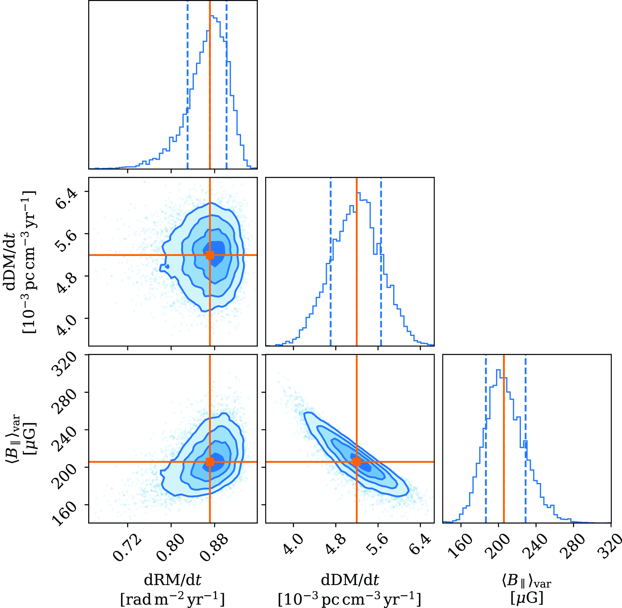
Posterior distributions for the piecewise linear model fit. The orange lines indicate the median and the blue dashed lines indicate the 16% and 84% percentiles of 1D posterior distributions. The contours indicate the 11.8%, 39.3%, 67.5%, and 86.4% percentiles of the 2D posterior distributions.
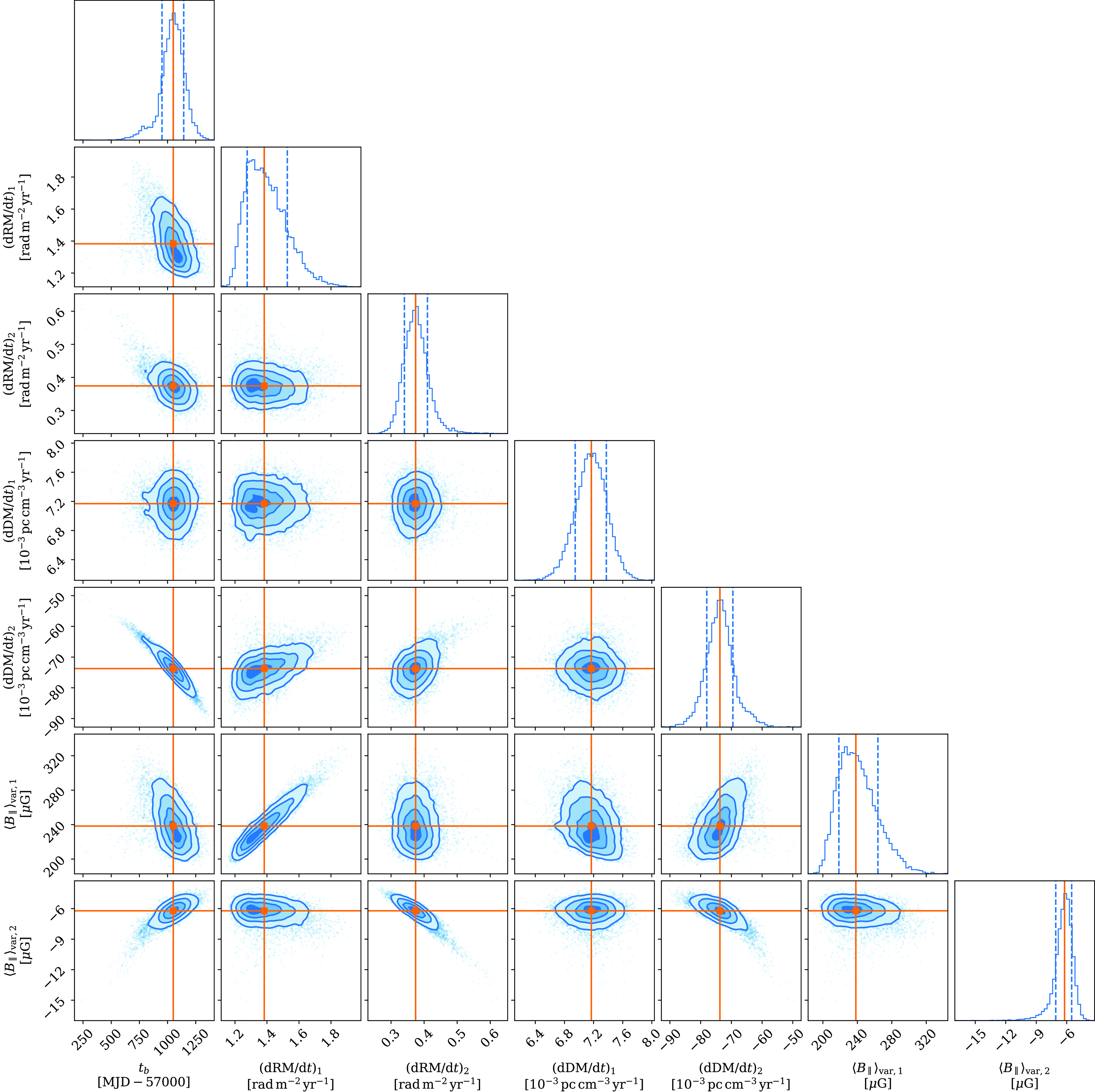
Since the dataset contains measurements from different telescopes at different observing frequencies, systematic errors will be inconsistent between publications. To address an analogous issue for pulsar flux density spectra, Jankowski et al. (Reference Jankowski, van Straten, Keane, Bailes, Barr, Johnston and Kerr2018) defined a robust log-likelihood which uses the Huber loss function to reduce the sensitivity to outlier data points (Huber Reference Huber1964). The robust log-likelihood is defined as
 \begin{equation} \log\mathcal{L}(y_i;t_i,\Theta) = -\sum_{i=1}^N \begin{cases} \frac{1}{2}\left(\frac{y_i-f(t_i;\Theta)}{\sigma_{y,i}}\right)^2 & \mathrm{if}\:\left|\frac{y_i-f(t_i;\Theta)}{\sigma_{y,i}}\right| < k \\[5pt] k\left|\frac{y_i-f(t_i;\Theta)}{\sigma_{y,i}}\right|-\frac{1}{2}k^2 & \mathrm{otherwise} \end{cases},\end{equation}
where
 $f(t_i;\Theta)$
is the model,
$f(t_i;\Theta)$
is the model,
 $\Theta$
are the model parameters,
$\Theta$
are the model parameters,
 $(t_i, y_i)$
are the data,
$(t_i, y_i)$
are the data,
 $\sigma_{y,i}$
are the uncertainties on
$\sigma_{y,i}$
are the uncertainties on
 $y_i$
, and k is a parameter defining the point at which outlier data points are penalised. Following Huber (Reference Huber1964), we used
$y_i$
, and k is a parameter defining the point at which outlier data points are penalised. Following Huber (Reference Huber1964), we used
 $k=1.345$
.
$k=1.345$
.
We jointly fit the RM and DM datasets by combining the likelihoods, forming a total likelihood
 \begin{equation} \log\mathcal{L} = \log\mathcal{L}_\mathrm{RM} + \log\mathcal{L}_\mathrm{DM}.\end{equation}
For the piecewise linear model,
 $\mathcal{L}_\mathrm{RM}$
and
$\mathcal{L}_\mathrm{RM}$
and
 $\mathcal{L}_\mathrm{DM}$
both depend on the break-point parameter
$\mathcal{L}_\mathrm{DM}$
both depend on the break-point parameter
 $t_b$
, so the RM and DM models are covariant.
$t_b$
, so the RM and DM models are covariant.
We used Bayesian inference to estimate the model parameters and their uncertainties. For the vertical intercepts and the break point, the priors were set to be uniform within the span of the dataset, and zero elsewhere. For the gradients
 $\mathrm{dRM}/\mathrm{d}t$
and
$\mathrm{dRM}/\mathrm{d}t$
and
 $\mathrm{dDM}/\mathrm{d}t$
, the priors were chosen to be uniform in the ranges
$\mathrm{dDM}/\mathrm{d}t$
, the priors were chosen to be uniform in the ranges
 $[{-}5,5]$
 $\mathrm{rad}\,\mathrm{m}^{-2}\,\mathrm{yr}^{-1}$
and
$\mathrm{rad}\,\mathrm{m}^{-2}\,\mathrm{yr}^{-1}$
and
 $[{-}0.5,0.5]$
 $\mathrm{cm}^{-3}\,\mathrm{pc}\,\mathrm{yr}^{-1}$
, respectively. We used the Dynesty dynamic nested sampler (Speagle Reference Speagle2020) integrated within Bilby (Ashton et al. Reference Ashton2019) to simultaneously estimate the Bayesian evidence and the posterior probability distribution. We then tested the sensitivity of the calculated evidence to the chosen priors by varying the size of the prior space.
$\mathrm{cm}^{-3}\,\mathrm{pc}\,\mathrm{yr}^{-1}$
, respectively. We used the Dynesty dynamic nested sampler (Speagle Reference Speagle2020) integrated within Bilby (Ashton et al. Reference Ashton2019) to simultaneously estimate the Bayesian evidence and the posterior probability distribution. We then tested the sensitivity of the calculated evidence to the chosen priors by varying the size of the prior space.
The posterior distributions of the fit parameters and
 $\langle B_\parallel \rangle_\mathrm{var}$
are shown in Figs. A1 and A2.
$\langle B_\parallel \rangle_\mathrm{var}$
are shown in Figs. A1 and A2.


 Open access