1. Introduction
Coronal mass ejections (CMEs) are the most dangerous source of space weather disturbances. They start suddenly and are in many cases unpredictable. Usually they are recorded after appearance in a field-of-view (FOV) of a space-borne coronagraph or in some cases of a ground-based coronagraph. The relation of CMEs to phenomena observed in the low corona is still under debates. Solar flares were initially considered as drivers of CMEs. However, later it was established that CMEs and flares are separate, while related phenomena (Webb & Howard Reference Webb and Howard2012). Whereas most energetic CMEs, as a rule, are associated with big flares, most flares occur independently of CMEs (Yashiro et al. Reference Yashiro, Gopalswamy, Akiyama, Michalek and Howard2005; Wang & Zhang Reference Wang and Zhang2007). In flare associated CME events, the CME onset typically precedes the associated X-ray flare onset by several minutes (Harrison Reference Harrison1991).
Statistical study shows that CMEs have the greatest correlation with eruptive prominences (filaments) among other near-surface activity (Munro et al. Reference Munro, Gosling, Hildner, MacQueen, Poland and Ross1979; St. Cyr & Webb Reference St. Cyr and Webb1991; Hori & Culhane Reference Hori and Culhane2002; Gopalswamy et al. Reference Gopalswamy, Shimojo, Lu, Yashiro, Shibasaki and Howard2003). Nevertheless, there is a difference in latitudinal distribution of CMEs and eruptive prominences. While at solar maximum both events can happen everywhere around the solar limb, close to minimum CMEs cluster around the solar equator, whereas eruptive prominences originate at latitudes typical for active regions (Plunkett et al. Reference Plunkett2002; Lozhechkin & Filippov Reference Lozhechkin and Filippov2004). This discrepancy can be explained by non-radial trajectories of eruptive prominences in the middle corona, which are observed in some well documented events (Gopalswamy et al. Reference Gopalswamy, Hanaoka and Hudson2000; Hori & Culhane Reference Hori and Culhane2002; Pevtsov et al. Reference Pevtsov, Panasenco and Martin2012; Panasenco et al. Reference Panasenco, Martin, Joshi and Srivastava2011, Reference Panasenco, Martin, Velli and Vourlidas2013) and follow from modeling (Filippov et al. Reference Filippov, Den and Geophys2001, 2002; Filippov Reference Filippov2016b). In some cases, eruptive prominences can be traced into the upper corona to become CME bright cores (House et al. Reference House, Wagner, Hildner, Sawyer and Schmidt1981; Illing & Athay Reference Illing and Athay1986; Gopalswamy et al. Reference Gopalswamy1998). Cold material evidently belonging to remnants of eruptive filaments is also detected within interplanetary CMEs (ICMEs), which are interplanetary manifestations of CMEs (Lepri & Zurbuchen Reference Lepri and Zurbuchen2010; Wang et al. Reference Wang, Feng and Zhao2018).
The CME speed in the FOV of space-borne coronagraphs varies in a wide range from tens km s−1 to more than 2500 km s−1, with an average value of about 500 km s−1 (Reference Gopalswamy, Poletto and SuessGopalswamy 2004). Sheeley et al. (Reference Sheeley, Walters, -M, Howard and Geophys1999) suggested to separate all CMEs into two types: gradual, or slow CMEs, which usually accelerate within the coronagraph FOV, and impulsive, or fast CMEs, which decelerate during propagation in the corona. CMEs with the speed lower than the average speed can be considered as slow, while the others are fast. Slow CMEs in most cases are associated with filament eruptions. Slow CMEs with persistently weak acceleration were known also as balloon-type events (Srivastava et al. Reference Srivastava, Schwenn, Inhester, Stenborg and Podlipnik1999, Reference Srivastava, Schwenn, Inhester, Martin and Hanaoka2000). Fast CMEs, in contrast, are usually related to solar flares. However, the separation of CMEs into two groups is rather conventional because parameters of flare-associated and non-flare CMEs considerably overlap (Vršnak et al. Reference Vršnak, Sudar and Ruždjak2005) and in most energetic events both flares and filament eruptions are observed (Schmieder et al. Reference Schmieder, Aulanier and Vršnak2015). Many researchers agree that one mechanism is sufficient to explain flare-related and prominence-related CMEs (Chen & Krall Reference Chen and Krall2003; Feynman & Ruzmaikin Reference Feynman and Ruzmaikin2004). Numerical simulations (Török & Kliem Reference Török and Kliem2007) confirmed the possibility to describe both slow and fast CMEs in a unified manner in a frame of a flux-rope model depending only on the structure of the overlying coronal magnetic field.
In this paper, we analyse 10 events initiated by filament eruptions, one part of which produced fast CMEs, while another was followed by slow CMEs. We estimate the initial store of free magnetic energy in all source regions to show the resemblance of pre-eruptive situations. On the basis of potential magnetic field calculations we come to conclusion that the difference of the late behaviour of eruptive prominences is a consequence of the different structure of magnetic fields above the filaments.
2. Two examples of filament eruptions and CMEs
2.1. 2013 September 29 event
Big quiescent filament erupted after 20:30 UT on 2013 September 29 (movie1). Full disc Hα image of the Sun taken at the Big Bear Solar Observatory (BBSO) with the big prominent filament stretched at an angle of about 10° with respect to the south-north direction is shown in Figure 1(a) just before the start of the eruption. We denote this filament by F1. The ends of the filament deviate to opposite sides from its rather straight body forming the inverse S-shaped structure typical for sigmoidal structures in the northern hemisphere (Rust & Kumar Reference Rust and Kumar1996; Pevtsov et al. Reference Pevtsov, Canfield and Latushko2001). Filament barbs are right-bearing and thin filament threads deviate clockwise from the filament axis. Both features indicate the dextral chirality of the filament in accordance with the hemispheric chirality rule (Martin et al. Reference Martin, Bilimoria, Tracadas, Rutten and Schrijver1994; Zirker et al. Reference Zirker, Martin, Harvey and Gaizauskas1997).
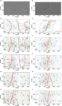
Full disc Hα images of the Sun on 2013 September 29 at 20:17:34 UT (a) and on 2016 January 26 at 11:34:15 UT (b). (Courtesy of Big Bear and Kanzelhoehe Solar Observatories).

The CME associated with the filament eruption [Figure 2(a)] appeared above the occulting disc of the Large Angle and Spectrometer Coronagraph (LASCO) C2 (Brueckner et al. Reference Brueckner1995) on board the Solar and Heliospheric Observatory (SOHO) at 22:12 UT. According to the SOHO/LASCO CME catalogue (http://cdaw.gsfc.nasa.gov/CME_list/), the CME moved with a linear speed of 1180 km s−1 and had a speed of 1165 km s−1 at a distance of 20 R ⊙ showing a constant speed. The core of the CME moved within the FOV of LASCO C2 with the averaged speed of 510 km s−1. The mass of the CME is estimated as 2.2×10¹⁶ g and the kinetic energy as 1.5×1032 erg, however these values are marked as rather uncertain. In the catalogue, the CME is characterised as a halo CME.
SOHO/LASCO C2 observations of the CMEs on 2013 September 29 (a) and 2016 January 26 (b). (Courtesy of the SOHO/LASCO Consortium, ESA and NASA).

2.2. 2016 January 26 event
Another filament eruption was observed on 2016 January 26 in the southern hemisphere (movie2). In Figure 1(b), the filament designated as F2 is shown in the full disc Hα filtergram of the Kanzelhoehe Solar Observatory 5 h before the eruption. The filament is stretched from the south-east to the north-west. Fine structure of the filament reveals the sinistral chirality typical for the southern hemisphere. The eruption starts at about 16:30 UT, and not all length of the filament was involved into the eruption. The eastern and western segments of the filament seem to hold their positions. Only the central section of the filament rises as a big loop. Some filament material falls to the filament ends and to an intermediate footpoint. Roudier et al. (Reference Roudier, Schmieder, Filippov, Chandra and Malherbe2018) studied triggers of this filament eruption. They concluded that the filament was destabilised by converging photospheric flows below it, which initiated an ascent of the middle section of the filament up to the critical height of the torus instability.
There are two CMEs which may be associated with the filament eruption according their time of appearance and position [Figure 2(b)]. The first CME appeared at 18:24 UT with the central position angle of 243°, a linear speed of 700 km s−1, and a speed of 820 km s−1 at a distance of 20 R ⊙ according to the SOHO/LASCO CME catalogue. The mass of the CME is estimated as 1.5×10¹⁵ g and the kinetic energy as 3.6×1030 erg. The second CME appeared at 19:24 UT with the central position angle of 235°, a linear speed of 320 km s−1, and a speed of 420 km s−1 at a distance of 20 R ⊙ according to the SOHO/LASCO CME catalogue. The core of the CME moved within the FOV of LASCO C2 with the averaged speed of 290 km s−1. The mass of this CME is estimated as 1.1×10¹⁵ g and the kinetic energy as 5.6×1029 erg. The observed CMEs could be launched by two independent events in the lower atmosphere, however there was not any other eruptive/flaring phenomenon in the south-west sector of the Earth-side solar hemisphere at convenient time. There was a small eruptive event observed on the far side of the Sun by the Solar Terrestrial Relations Observatory Ahead (STEREO A), which was at that time nearly diametrically opposite the Earth. The eruption was located in the south-west sector of the disc in the framework of STEREO A, which was appropriate for the source region of the observed CMEs, but it began at 20 UT, too late to be the source of each CME.
We believe that both CMEs are parts of the same event. The first CME represents the frontal structure, while the second one corresponds to the core of the CME. As usual, the frontal structure moves faster than the core. Linear extrapolation of the height-time plots of both CMEs in the SOHO/LASCO CME catalogue shows the same start time about 18 UT. Of course, this estimation gives a little retarded start time because does not take into account the acceleration of a CME at the beginning of an eruption and the distance from the source region to the limb. Nevertheless, this is in accordance with the beginning of the filament eruption at about 16:30 UT.
3. Energy of filament electric currents
The two filaments were similar in size and erupted in similar ways, but produced very different CMEs. At first we compare the initial conditions of the pre-eruptive filaments. Both filaments were located between large-scale areas of opposite magnetic polarities (compare Figures 1 and 3). Following a flux-rope model of the filament magnetic structure we can estimate the total initial electric currents associated with both filaments and the initial magnetic energies.
In the simplest model with the flux rope considered as a straight linear current, the vertical equilibrium is described as (van Tend & Kuperus Reference van Tend and Kuperus1978; Molodenskii & Filippov Reference Molodenskii and Filippov1987; Priest & Forbes Reference Priest and Forbes1990)
 $$
{{I^2 } \over {c^2 h}} - {I \over c}B_t (h) - mg = 0,
$$
$$
{{I^2 } \over {c^2 h}} - {I \over c}B_t (h) - mg = 0,
$$
where I is the total electric current, h is the height of the electric current above the photosphere, B t is the horizontal component of the surrounding magnetic field, m is the mass of the tube per unit length, g is the free fall acceleration. Neglecting gravitation when compared with magnetic forces, we can estimate the strength of the total electric current
 $$I = chB_t .$$
Of course, we cannot obtain both needed values directly from observations but we can estimate them using potential field calculations. We cut some rectangular areas surrounding the filaments from the full-disc magnetograms (Figure 3) and transform it into array with pixels of equal area. The obtained image looks like if it is observed at the centre of the solar disk. We use the modified array as the boundary conditions for solving the Neumann external boundary-value problem (see Filippov Reference Filippov2013 and references therein).
SDO/HMI images of the line-of-sight magnetic field on 2013 September 29 (a) and on 2016 January 26 (b). (Courtesy of the SDO/HMI Consortium, ESA and NASA).
Figure 4 presents the results of potential field calculations. Two top rows show clipped portions of Hα filtergrams and magnetograms transformed into equal-area-pixel arrays. In the middle row, PILs at different heights are superposed on the Hα images. The PILs are drawn taking into account the projection effect, so PILs touching the spines of filaments correspond to their heights (Filippov Reference Filippov2016c,a). The height of the filament F1 is between 60 and 84 Mm, while the height of the filament F2 is between 36 and 48 Mm. Figure 4(d) and 4(i) shows the distribution of the decay index (Bateman Reference Bateman1978; Filippov & Den Reference Filippov and Den2000, Reference Filippov, Den and Geophys2001; Kliem & Török Reference Kliem and Török2006)
 $$
n = - {{\partial \ln B_t } \over {\partial \ln h}},
$$
$$
n = - {{\partial \ln B_t } \over {\partial \ln h}},
$$
at heights where the contours n = 1 touch PILs. These heights can be considered as critical heights h c from which filaments start to erupt (van Tend & Kuperus Reference van Tend and Kuperus1978; Filippov & Den Reference Filippov and Den2000, Reference Filippov and Den2001; Démoulin & Aulanier Reference Démoulin and Aulanier2010; Olmedo & Zhang Reference Olmedo and Zhang2010). There are other estimations for the threshold of eruptive instability. A toroidal current ring becomes unstable if n = 1.5 (Bateman Reference Bateman1978; Kliem & Török Reference Kliem and Török2006). The anchoring of the flux-rope ends in the photosphere (Olmedo & Zhang Reference Olmedo and Zhang2010) and taking into account its finite cross-section (Démoulin & Aulanier Reference Démoulin and Aulanier2010) reduce the critical value of the decay index n c to close vicinity of unity. The majority of studies of the onset of filament eruptions (Filippov & Zagnetko Reference Filippov and Zagnetko2008; McCauley et al. Reference McCauley, Su, Schanche, Evans, Su, McKillop and Reeves2015; Zuccarello et al. Reference Zuccarello, Seaton, Mierla, Poedts, Rachmeler, Romano and Zuccarello2014a,Reference Zuccarello, Seaton, Filippov, Mierla, Poedts, Rachmeler, Romano and Zuccarellob) show that filaments begin to accelerate abruptly when they reach the region with the decay index value close to unity.
Left column: the fragment of the Hα filtergram on 2013 September 29 at 20:18 UT (a), the corresponding fragment of the magnetogram (b), PILs at different heights superposed on the Hα filtergram (c), the distribution of the decay index at the height of 82 Mm (d), and the distribution of the horizontal field component at the height of 82 Mm (e). Right column: the same for 2016 January 26 at 11:34 UT and the height of 60 Mm.
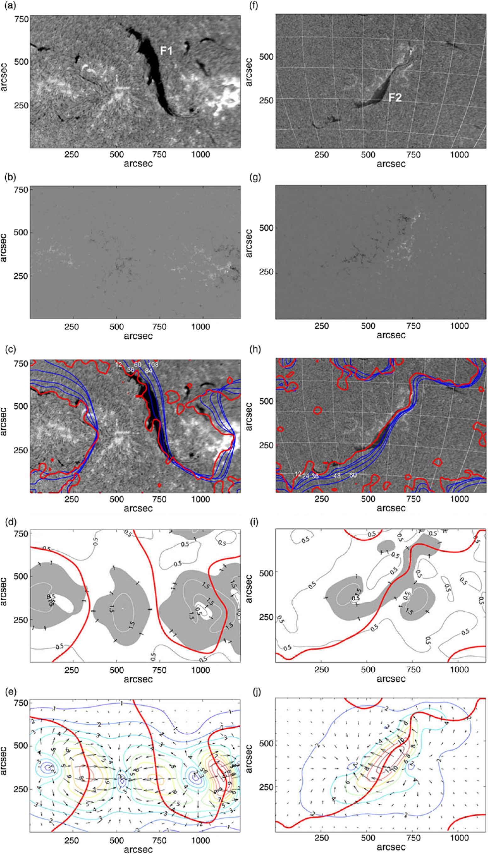
On September 29, the critical height h c is 82 Mm. It is close to the height estimated from Figure 4(c). Really, the filament starts to rise soon after the shown moment 20:18 UT. The critical height for the filament F2 is 60 Mm. It is greater than estimated height in Figure 4(h). However, the filament in this image is shown at the moment about 5 h before the eruption and is able to rise slowly to a greater height. Thus, the value of the critical height seems reasonable.
The bottom row of Figure 4 shows distributions of the horizontal field component B t at the critical heights. The direction of B t shown by arrows corresponds to the direction from positive to negative polarity in the photosphere below the filaments. Maximum values of the horizontal field are about 7 G at the height of 82 Mm on September 29 and 12 G at the height of 60 Mm on January 26. Substituting these values into formula (2), we obtain the strength of the total electric currents as 5.7×10¹¹ A and 7.2×10¹¹ A, respectively.
The magnetic energy of an electric current is expressed as (Tamm Reference Tamm1966)
 $$
W = {{LI^2 } \over {2c^2 }},
$$
$$
W = {{LI^2 } \over {2c^2 }},
$$
where L is the inductance of the circuit. The inductance of the line currents is approximately equal to their lengths. The length of the filament F1 in Figure 4(a) is about 430 Mm, while the length of the continuous part of the filament F2 in Figure 4(f) is about 290 Mm. If we take into account the whole length of filaments including thin faint ends and intermediate gaps, F1 is 500 Mm and F2 is 470 Mm long. Then the magnetic energy related to F1 is between 7×1031 erg and 8×1031 erg. The energy related to F2 is between 7.5×1031 erg and 12×1031 erg. Parameters of the filaments F1 and F2 are presented in Tables 1 and 2 along with parameters of other eight filaments associated with fast and slow CMEs.
Eruptive filaments associated with fast CMEs.

Eruptive filaments associated with slow CMEs.
Our estimations of the electric current strength and the whole magnetic energy show that both filaments are similar in these parameters characterising the initial conditions with values for F2 a little greater, but F1 produced a fast CME, while F2 initiated a slow CME. To find the reason for different erupting filament behaviour we should consider the structure of the coronal magnetic field above the filaments where the filaments accelerate.
4. Structure of the potential magnetic field in the source regions
To analyse the structure of the coronal magnetic field above the filaments, we use magnetograms taken 2 days before the eruptive events when the regions were close to the central meridian. The large-scale structure of the field does not change significantly from day to day, while measurements of the magnetic field in the region when it is near the central meridian are more accurate and reliable. The results are shown in Figure 5. The top row shows clipped portions of magnetograms used as boundary conditions. The second row presents distributions of the horizontal field component B t at the critical heights which are practically identical to Figure 4(e) and 4(j) for the days of eruptions. The position of the filaments is shown as green contours. At the heights of 200 and 300 Mm, the horizontal field above the filament F2 is 2–4 times greater than that above the filament F1. At the heights of 400 and 500 Mm, the field above the filament F2 is still slowly decreasing, while the field above the filament F1 changes direction to opposite. The horizontal field above 350 Mm does not hold the filament more but pushes it away from the solar surface. The filament receives additional acceleration and transforms into the fast CME. Despite the smaller initial electric current, the filament F1 is surrounded by a weaker holding magnetic field which decreases rapidly with height and changing the direction to opposite becomes an accelerating field.
Left column: the fragment of the SDO/HMI magnetogram on 2013 September 27 at 20:12 UT (a) and the distribution of the horizontal field component at different heights (b)–(f). Right column: the same for 2016 January 24 at 08:13 UT. Thick red lines show PILs at the corresponding heights. Green contours in the frames (b) and (h) indicate positions of filaments.
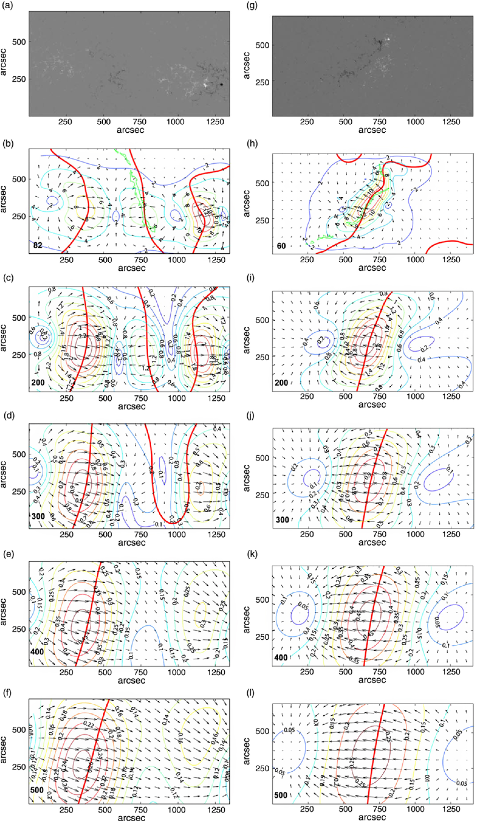
The difference in the coronal magnetic field behaviour with height is based on different distributions of photospheric fields. The region near the filament F2 has two large-scale areas of opposite polarities [Figure 5(g)]. Thus, the structure of the coronal field can be considered as more or less dipolar. The field falls with height not faster than inverse cubic distance from the centre of an effective dipole. The photospheric field around the filament F1 is more complicated. It contains at least four magnetic cells [Figure 5(a)] less spacious than cells in Figure 5(g). The coronal magnetic field is more like quadrupolar one and therefore decreases with height faster than dipolar field. It can contain a null point at some height and can change direction to opposite on the other side of the null as we see in Figure 5.
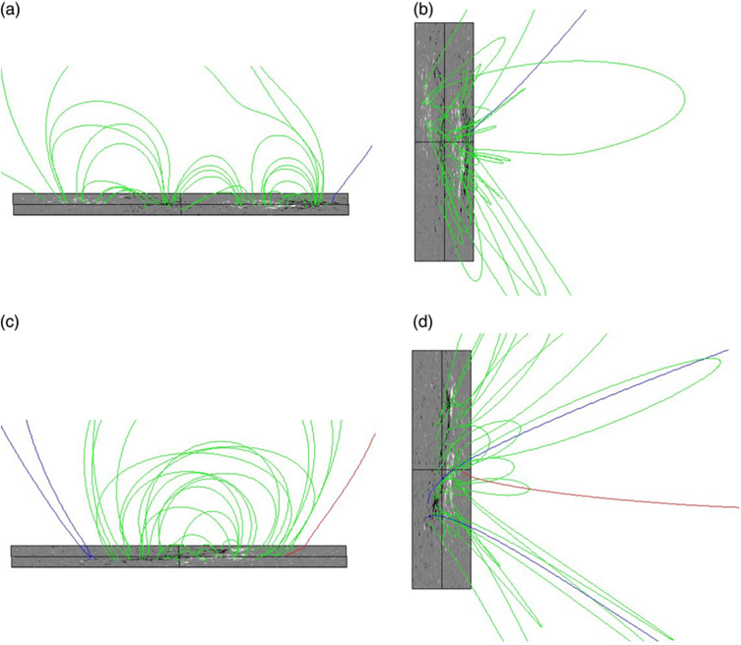
Figure 6 shows the structure of potential field lines above the filaments F1 and F2. Left panels present the view form the south, right panels show the view from the east, as it is expected at the western limb. Field lines above the filament F2 are similar to a simple bipolar arcade, while in the southern view of the region with the filament F1 the quadrupolar structure is clearly visible. A saddle-like geometry above the central loop system indicates the presence of a null point.
Structure of potential field lines above the filaments F1 (upper row) and F2 (bottom row).
We analysed additionally four filament eruptions associated with fast CMEs and four eruptions associated with slow CMEs. The results are presented in Tables 1 and 2. The thirdcolumn presents values of the horizontal component of potential field B t at the critical height h c shown in the next column. The sixth column presents filament lengths measured in filtergrams. Estimations of the electric current strength I and magnetic energy W according expressions (2) and (4) are shown in the fifth and seventh columns. The eighth column presents angles α between the horizontal directions of the potential magnetic field at the heights of 10 Mm and of 600 Mm. In the last column, linear speeds of the associated CMEs from the SOHO/LASCO CME catalogue are presented. The parameters of the filaments F1 and F2 are shown in the last lines of both tables. On account of many uncertainties in data, all values in tables should be considered as estimations with errors no less than 50%.
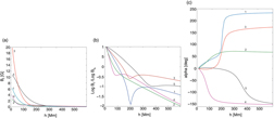
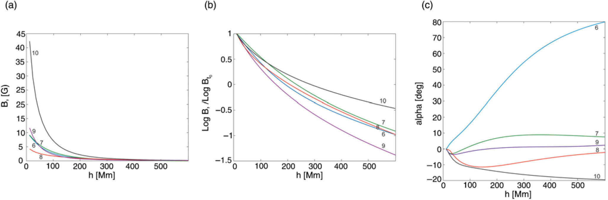
The behaviours of the potential magnetic field above the filaments are shown in Figures 7 and 8 for fast and slow CMEs, respectively. The profiles are calculated along the radial direction starting from the height of 10 Mm near the centre of a filament up to the height of 600 Mm. Every curve is labelled with a figure corresponding to the number of event in Tables 1 and 2. The panels 7(a) and 8(a) show the decrease of horizontal field with height. The behavior of the field is better seen in the panels 7(b) and 8(b) presenting the value logB t/logB t0, where B t0 is the value at the height of 10 Mm. The panels 7(c) and 8(c) show the rotation of the horizontal field with height.
Height profiles of the horizontal component B t of the potential magnetic field (a), the value of LogB t/LogB t , and the angle of the horizontal field rotation α above filaments, which initiated fast CMEs.
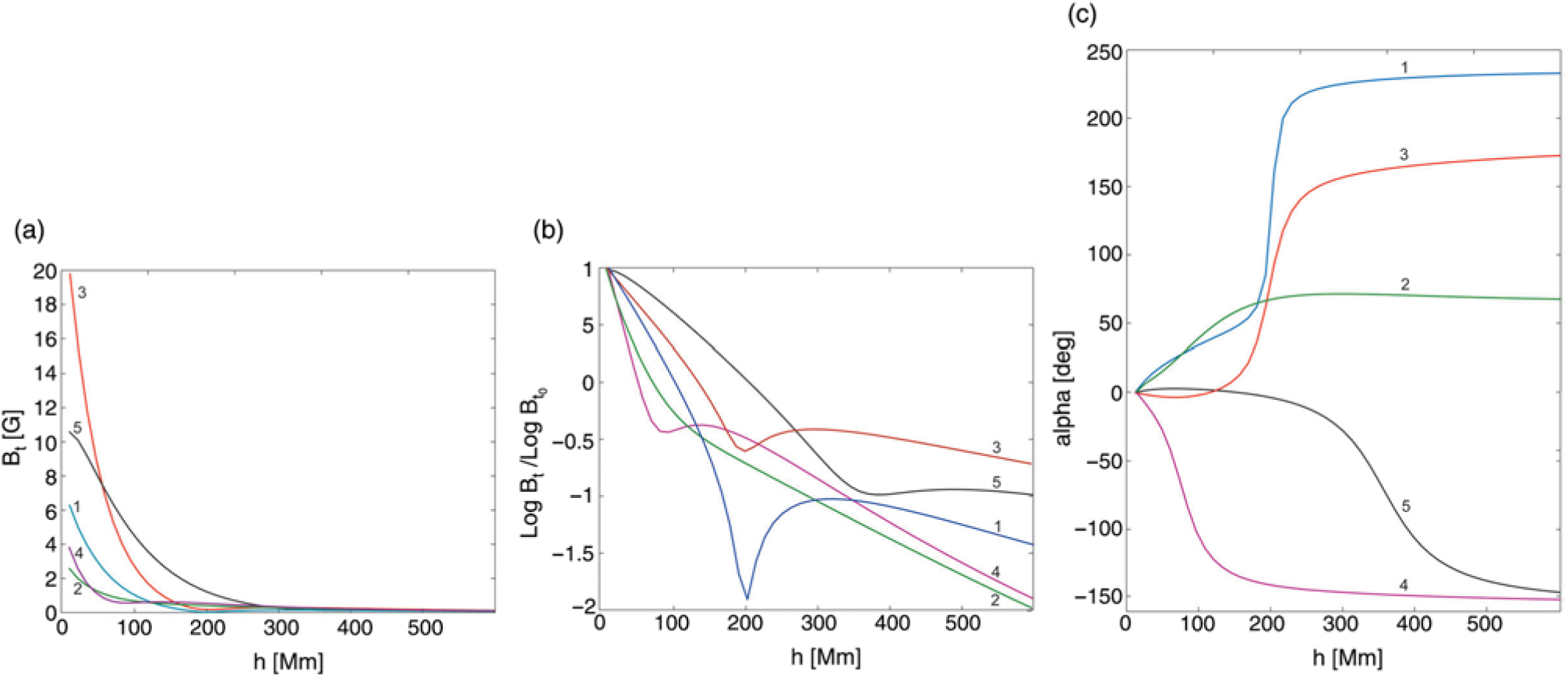
Comparison of Tables 1 and 2 does not demonstrate significant difference in values of electric current and magnetic energy for filaments associated with fast and slow CMEs, while they vary from event to event in each family. However, the values of α in the eighth column are quite different in the two tables. It is clearly visible in Figures 7(c) and 8(c). Rotation of the field to an angle of order of 180° indicates the presence of a quadrupolar structure with a null point. The influence of the nearby null point is manifested in dips on the curves in Figure 7(b) suggesting the reduction of the field in the vicinity of the null. Only one curve has no a dip. This curve corresponds to the not very fast event (570 km s−1). Nevertheless, the field slopes down faster than any one in Figure 8(b).
The same as in Figure 7 for regions producing slow CMEs.
The results of our analysis are consistent with the numerical simulations (Török & Kliem Reference Török and Kliem2007) of flux-rope eruptions in bipolar and quadrupolar active regions. Török & Kliem (Reference Török and Kliem2007) showed that the accelerations profile of the erupting flux rope depends on the steepness of the coronal field decrease with height. The fastest CMEs are expected in most complex active regions.
There are several simplifications used in our analysis. They, of course, limit the accuracy of some quantitative results. We do not take into account the internal structure of flux ropes containing the filaments and use a simple model with a straight linear current. It seems reasonable because we analyse the equilibrium of the flux rope as a whole and correlate the axis of the flux rope with the filament spine. We consider the photospheric boundary as a flat surface, which is not the case for such large areas. Thus, the contribution of sources from the periphery of the areas is accounted not very correctly. Nevertheless, our calculations are more or less correct for the central part of the area up to heights less than the width of the box.
5. Summary and conclusions
We analysed 10 filament eruptions, one part of which was associated with fast CMEs, while the other was followed by slow CMEs. Particular attention has been given to two big long-living quiescent filaments nearly of the same size located far from active regions. First eruption happened on 2013 September 29 in the northern hemisphere. It started at 20:30 UT as slow rising of the filament (F1) with continues and increasing acceleration. The eruption produced a big halo CME with the frontal structure moving in the FOV of SOHO/LASCO with a constant speed of about 1200 km s−1. The core of the CME moved within the FOV of LASCO C2 with the averaged speed of 510 km s−1. The other filament (F2) erupted on 2016 January 26 at about 16:30 UT in the southern hemisphere. It was associated with a slower CME. The frontal structure of the CME moved with a speed changing from 700 to 800 km s−1. The core of the CME propagated within the FOV of LASCO C2 with the averaged speed of 290 km s−1. As usual the frontal structure moves faster than the core because the flux rope, which forms a CME, moves translationally and in addition simultaneously expands.
Our estimations of the electric current strength and the whole magnetic energy show that both filaments are similar in these parameters characterising the initial conditions with values for F2 a little greater. However, F1 produced a fast CME, while F2 initiated a slow CME. We ascribe the difference of the late behaviour of the two eruptive prominences to the different structure of magnetic field above the filaments. The structure of the coronal field above the filament F2 can be considered as more or less dipolar. The field falls with height not faster than inverse cubic distance from the centre of an effective dipole. The field retards the filament acceleration even at great heights. The coronal magnetic field above the filament F1 is more like quadrupolar one and therefore decreases with height much faster than the dipolar field. It contains a null point at some height and changes direction to opposite on the other side of the null to create additional accelerating force for the filament ascending.
Similar structures were found in other four regions, which produced fast CMEs. Most conspicuous feature is the changing of the horizontal field direction to nearly opposite with the increase of height. Such behavior is natural, if one moves near a magnetic null point. The results of our analysis are consistent with the numerical simulations (Török & Kliem Reference Török and Kliem2007) of flux-rope eruptions in bipolar and quadrupolar active regions.
Acknowledgements
The author thanks the Big Bear and Kanzelhoehe Solar Observatories, SOHO/LASCO, SDO/AIA, SDO/HMI science teams for the high-quality data supplied. The author is grateful to the anonymous referee whose suggestions and comments significantly improved this paper.