


1 Introduction
To each parabolic Coxeter system,
 $(W,P)$
, we have an associated family of “anti-spherical Kazhdan–Lusztig polynomials”,
$(W,P)$
, we have an associated family of “anti-spherical Kazhdan–Lusztig polynomials”,
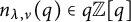
 $n_{\lambda ,\nu }(q)$
, indexed by pairs of cosets for
$n_{\lambda ,\nu }(q)$
, indexed by pairs of cosets for
 $P\leq W$
. These polynomials are some of the most important combinatorial objects in Lie theory and representation theory and they can be computed (at least in theory) via a recursive, non-positive formula. Deodhar proposed a (non-recursive!) combinatorial approach to studying these polynomials in [Reference DeodharDeo90].
$P\leq W$
. These polynomials are some of the most important combinatorial objects in Lie theory and representation theory and they can be computed (at least in theory) via a recursive, non-positive formula. Deodhar proposed a (non-recursive!) combinatorial approach to studying these polynomials in [Reference DeodharDeo90].
Libedinsky–Williamson categorified the anti-spherical Kazhdan–Lusztig polynomials by interpreting them as composition factor multiplicities of simple modules within standard modules for the anti-spherical Hecke category,
 $\mathcal {H}_{(W,P)}$
[Reference Libedinsky and WilliamsonLW]. In more detail: we first fix a reduced word
$\mathcal {H}_{(W,P)}$
[Reference Libedinsky and WilliamsonLW]. In more detail: we first fix a reduced word
 $\underline {\mu }$
for each
$\underline {\mu }$
for each
 $\mu \in {^PW}$
, for
$\mu \in {^PW}$
, for
 $\lambda \in {^PW}$
the standard
$\lambda \in {^PW}$
the standard
 $\mathcal {H}_{(W,P)}$
-module
$\mathcal {H}_{(W,P)}$
-module
 $\Delta (\lambda )$
has light leaves basis enumerated by
$\Delta (\lambda )$
has light leaves basis enumerated by
 $\cup _{\mu \in {^PW}}\mathrm {Path}(\lambda ,\underline {\mu })$
the set of all paths (or “Bruhat strolls”) in the coset graph for
$\cup _{\mu \in {^PW}}\mathrm {Path}(\lambda ,\underline {\mu })$
the set of all paths (or “Bruhat strolls”) in the coset graph for
 $(W,P)$
which terminate at
$(W,P)$
which terminate at
 $\lambda $
such that the steps in these paths are “coloured by”
$\lambda $
such that the steps in these paths are “coloured by”
 $\underline {\mu }$
. This basis is graded according to the degree statistic for the underlying paths, we record this in the matrix
$\underline {\mu }$
. This basis is graded according to the degree statistic for the underlying paths, we record this in the matrix
 $$\begin{align*}\Delta^{(W,P)}:=( \Delta_{\lambda,\underline{\mu}}(q))_{\lambda,\mu\in {{^P}W}} \qquad \qquad \Delta_{\lambda,\underline{\mu}}(q)=\sum_{\mathsf{S} \in \mathrm{Path}(\lambda,\underline{\mu})}\!\!\!\!\!\! q^{\deg(\mathsf{S})} \end{align*}$$
which is a (square) lower uni-triangular matrix. This matrix can be factorized uniquely as a product of lower uni-triangular matrices
 $$\begin{align*}N^{(W,P)}:=(n_{\lambda,\nu}(q))_{\lambda,\nu\in {{^P}W}} \qquad B^{(W,P)}:=(b_{\nu,\underline{\mu}}(q))_{\nu,\mu\in {{^P}W}} \end{align*}$$
such that
 $n_{\lambda ,\nu }(q)\in q{\mathbb Z}[q]$
for
$n_{\lambda ,\nu }(q)\in q{\mathbb Z}[q]$
for
 $\lambda \neq \nu $
and
$\lambda \neq \nu $
and
 $b_{\nu ,\underline {\mu }}(q)\in {\mathbb Z}[q+q^{-1}]$
. The polynomial
$b_{\nu ,\underline {\mu }}(q)\in {\mathbb Z}[q+q^{-1}]$
. The polynomial
 $n_{\lambda ,\nu }(q)$
is the anti-spherical Kazhdan–Lusztig polynomial for
$n_{\lambda ,\nu }(q)$
is the anti-spherical Kazhdan–Lusztig polynomial for
 $\lambda \leq \nu \in {^PW}$
. Over the complex field, the polynomial
$\lambda \leq \nu \in {^PW}$
. Over the complex field, the polynomial
 $n_{\lambda ,\nu }(q)$
counts the graded composition factor multiplicity
$n_{\lambda ,\nu }(q)$
counts the graded composition factor multiplicity
 $[\Delta (\lambda ):L(\nu )]$
and the polynomials
$[\Delta (\lambda ):L(\nu )]$
and the polynomials
 $b_{\nu ,\underline {\mu }}(q)$
describe the graded character of the simple module
$b_{\nu ,\underline {\mu }}(q)$
describe the graded character of the simple module
 $L(\nu )$
[Reference Elias and WilliamsonEW14, Reference Libedinsky and WilliamsonLW]. This provides an innately positive interpretation of the coefficients of the polynomial
$L(\nu )$
[Reference Elias and WilliamsonEW14, Reference Libedinsky and WilliamsonLW]. This provides an innately positive interpretation of the coefficients of the polynomial
 $n_{\lambda ,\nu }(q)$
and thus proves the famous Kazhdan–Lusztig positivity conjecture [Reference Elias and WilliamsonEW14] and its anti-spherical counterpart [Reference Libedinsky and WilliamsonLW].
$n_{\lambda ,\nu }(q)$
and thus proves the famous Kazhdan–Lusztig positivity conjecture [Reference Elias and WilliamsonEW14] and its anti-spherical counterpart [Reference Libedinsky and WilliamsonLW].
Libedinsky–Williamson proposed that this extra
 $\mathcal {H}_{(W,P)}$
-structure should provide new insight toward Deodhar’s goal of a counting formula for the Kazhdan–Lusztig polynomials. They ask in [Reference Libedinsky and WilliamsonLW21, Problem 1.2] whether it is possible to construct an explicit basis of “canonical light leaves” for a
$\mathcal {H}_{(W,P)}$
-structure should provide new insight toward Deodhar’s goal of a counting formula for the Kazhdan–Lusztig polynomials. They ask in [Reference Libedinsky and WilliamsonLW21, Problem 1.2] whether it is possible to construct an explicit basis of “canonical light leaves” for a
 ${\mathbb Z}$
-module
${\mathbb Z}$
-module
 $\mathbb N_{\lambda ,\underline \nu }$
whose graded rank is equal to
$\mathbb N_{\lambda ,\underline \nu }$
whose graded rank is equal to
 $n_{\lambda ,\nu }(q)$
. Each canonical light leaf basis element of degree k would then be a generator of some composition factor of
$n_{\lambda ,\nu }(q)$
. Each canonical light leaf basis element of degree k would then be a generator of some composition factor of
 $\Delta (\lambda )$
isomorphic to
$\Delta (\lambda )$
isomorphic to
 $L(\nu )\langle k \rangle $
. We solve this problem in the case of Hermitian symmetric pairs (see Figure 1) by introducing an oriented Temperley–Lieb algebra of type
$L(\nu )\langle k \rangle $
. We solve this problem in the case of Hermitian symmetric pairs (see Figure 1) by introducing an oriented Temperley–Lieb algebra of type
 $(W,P)$
for all Hermitian symmetric pairs
$(W,P)$
for all Hermitian symmetric pairs
 $(W,P)$
.
$(W,P)$
.
Theorem A Let
 $(W,P)$
be a Hermitian symmetric pair. For all
$(W,P)$
be a Hermitian symmetric pair. For all
 $\lambda , \nu \in {^PW}$
, the space
$\lambda , \nu \in {^PW}$
, the space
 $\mathbb N_{\lambda ,\underline \nu }$
has basis indexed by the set of “standard” basis elements in the anti-spherical module for the oriented Temperley–Lieb algebra of type
$\mathbb N_{\lambda ,\underline \nu }$
has basis indexed by the set of “standard” basis elements in the anti-spherical module for the oriented Temperley–Lieb algebra of type
 $(W,P)$
. These elements can be described in a closed combinatorial (non-iterative) fashion. Moreover, this construction is entirely independent of the choice of a reduced word
$(W,P)$
. These elements can be described in a closed combinatorial (non-iterative) fashion. Moreover, this construction is entirely independent of the choice of a reduced word
 $\underline {\nu }$
.
$\underline {\nu }$
.
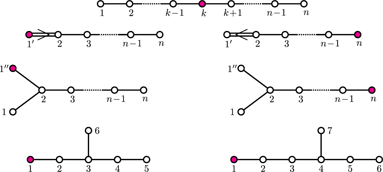
Enumeration of nodes in the parabolic Dynkin diagram of the Hermitian symmetric pairs. Namely, types
 $(A_{n }, A_{k-1} \times A_{n-k } )$
,
$(A_{n }, A_{k-1} \times A_{n-k } )$
,
 $(C_n, A_{n-1}) $
and
$(C_n, A_{n-1}) $
and
 $(B_n, B_{n-1}) $
,
$(B_n, B_{n-1}) $
,
 $(D_{n+1} , A_{n}) $
and
$(D_{n+1} , A_{n}) $
and
 $(D_{n+1}, D_{n }) $
and
$(D_{n+1}, D_{n }) $
and
 $(E_6 , D_5 ) $
and
$(E_6 , D_5 ) $
and
 $(E_7 , E_6), $
respectively. The single node not belonging to the parabolic is highlighted in pink in each case.
$(E_7 , E_6), $
respectively. The single node not belonging to the parabolic is highlighted in pink in each case.
The use of Temperley–Lieb style combinatorics for calculating Kazhdan–Lusztig polynomials goes back to work of Brundan and Stroppel in type
 $(A_n, A_k\times A_{n-k-1})$
[Reference Brundan and StroppelBS10, Reference Brundan and StroppelBS11a, Reference Brundan and StroppelBS11b, Reference Brundan and StroppelBS12] and Cox and De Visscher in type
$(A_n, A_k\times A_{n-k-1})$
[Reference Brundan and StroppelBS10, Reference Brundan and StroppelBS11a, Reference Brundan and StroppelBS11b, Reference Brundan and StroppelBS12] and Cox and De Visscher in type
 $(D_n, A_{n-1})$
[Reference Cox and De VisscherCD11]. In this paper, we generalize these ideas to all Hermitian symmetric pairs and lift the combinatorics to a higher structural level; we do this by interpreting these polynomials as graded-dimensions of “anti-spherical modules” for oriented Temperley–Lieb algebras of type
$(D_n, A_{n-1})$
[Reference Cox and De VisscherCD11]. In this paper, we generalize these ideas to all Hermitian symmetric pairs and lift the combinatorics to a higher structural level; we do this by interpreting these polynomials as graded-dimensions of “anti-spherical modules” for oriented Temperley–Lieb algebras of type
 $(W,P)$
. The definition of these algebras and their anti-spherical modules is simple and uniformly given in terms of the underlying root system, see Definitions 3.3 and 3.9. We also relate these newly defined oriented Temperley–Lieb algebras of type
$(W,P)$
. The definition of these algebras and their anti-spherical modules is simple and uniformly given in terms of the underlying root system, see Definitions 3.3 and 3.9. We also relate these newly defined oriented Temperley–Lieb algebras of type
 $(W,P)$
to the generalized Temperley–Lieb algebras of type W introduced by Fan and Graham. In Section 4, we give a proof of Theorem A for types
$(W,P)$
to the generalized Temperley–Lieb algebras of type W introduced by Fan and Graham. In Section 4, we give a proof of Theorem A for types
 $(D_n, D_{n-1})$
,
$(D_n, D_{n-1})$
,
 $(B_n, B_{n-1})$
and the exceptional types
$(B_n, B_{n-1})$
and the exceptional types
 $(E_6, D_5)$
and
$(E_6, D_5)$
and
 $(E_7, E_6)$
. From Section 5 onwards we focus solely on the remaining types, namely,
$(E_7, E_6)$
. From Section 5 onwards we focus solely on the remaining types, namely,
 $(W,P)=(A_n, A_k\times A_{n-k-1})$
,
$(W,P)=(A_n, A_k\times A_{n-k-1})$
,
 $(D_n, A_{n-1}),$
and
$(D_n, A_{n-1}),$
and
 $(C_n, A_{n-1})$
. In Section 6, we prove that the oriented Temperley–Lieb algebras admit a diagrammatic visualization, and use this in Section 7 to understand the graded structure of the algebra by way of closed combinatorial formulas. In Section 8, we apply these ideas to the anti-spherical module and hence prove Theorem A for the remaining types.
$(C_n, A_{n-1})$
. In Section 6, we prove that the oriented Temperley–Lieb algebras admit a diagrammatic visualization, and use this in Section 7 to understand the graded structure of the algebra by way of closed combinatorial formulas. In Section 8, we apply these ideas to the anti-spherical module and hence prove Theorem A for the remaining types.
Further rewards of our approach will be harvested in the companion paper [Reference Bowman, De Visscher, Hazi and NortonBDHN]. In [Reference Bowman, De Visscher, Hazi and NortonBDHN], we establish isomorphisms interrelating Hecke categories and use these isomorphisms in order to construct the basic algebras of these Hecke categories and prove that they are standard Koszul (this uses the results of this paper in order to deduce the required graded vector space dimension counts) and to prove that the p-Kazhdan–Lusztig polynomials are entirely independent of the prime
 $p\geq 0$
.
$p\geq 0$
.
2 Kazhdan–Lusztig polynomials and Deodhar’s defect
Let
 $(W, S_W)$
be a Coxeter system: W is the group generated by the finite set
$(W, S_W)$
be a Coxeter system: W is the group generated by the finite set
 $S_W$
subject to the relations
$S_W$
subject to the relations
 $(st)^{m_{st}} = 1$
for
$(st)^{m_{st}} = 1$
for
 $s,t\in S_W$
,
$s,t\in S_W$
,
 $ {m_{st}}\in {\mathbb N}\cup \{\infty \}$
satisfying
$ {m_{st}}\in {\mathbb N}\cup \{\infty \}$
satisfying
 ${m_{st}}= {m_{ts}}$
, and
${m_{st}}= {m_{ts}}$
, and
 ${m_{st}}=1$
if and only if
${m_{st}}=1$
if and only if
 $s= t$
. Let
$s= t$
. Let
 $\ell : W \to \mathbb {N}$
be the corresponding length function. Consider
$\ell : W \to \mathbb {N}$
be the corresponding length function. Consider
 $S_P \subseteq S_W$
a subset and
$S_P \subseteq S_W$
a subset and
 $(P, S_P)$
its corresponding Coxeter system. We say that P is the parabolic subgroup corresponding to
$(P, S_P)$
its corresponding Coxeter system. We say that P is the parabolic subgroup corresponding to
 $S_P\subseteq S_W$
. Let
$S_P\subseteq S_W$
. Let
 $^ PW \subseteq W$
denote a set of minimal length coset representatives in
$^ PW \subseteq W$
denote a set of minimal length coset representatives in
 $P\backslash W$
. For
$P\backslash W$
. For
 ${\underline {w}}=s_{i_1}s_{i_2}\cdots s_{i_\ell }$
an expression in the generators
${\underline {w}}=s_{i_1}s_{i_2}\cdots s_{i_\ell }$
an expression in the generators
 $s_{i_j} \in S_W$
for
$s_{i_j} \in S_W$
for
 $0\leq j \leq \ell $
, we define a subexpression of
$0\leq j \leq \ell $
, we define a subexpression of
 $\underline {w}$
to be an expression of the form
$\underline {w}$
to be an expression of the form
 ${\underline {w}}^{\underline {k}} :=s_{i_1}^{k_1}s_{i_2}^{k_2}\cdots s_{i_\ell }^{k_\ell }$
where
${\underline {w}}^{\underline {k}} :=s_{i_1}^{k_1}s_{i_2}^{k_2}\cdots s_{i_\ell }^{k_\ell }$
where
 $\underline {k}=(k_1,k_2,\dots ,k_\ell )\in \{0,1\}^\ell $
. We let
$\underline {k}=(k_1,k_2,\dots ,k_\ell )\in \{0,1\}^\ell $
. We let
 $\leq $
denote the (strong) Bruhat order on
$\leq $
denote the (strong) Bruhat order on
 ${^PW}$
: namely
${^PW}$
: namely
 $y\leq w$
if for some reduced expression
$y\leq w$
if for some reduced expression
 ${\underline {w}}$
for w, there exists a reduced expression
${\underline {w}}$
for w, there exists a reduced expression
 ${\underline {y}}$
for y such that
${\underline {y}}$
for y such that
 ${\underline {y}}$
is a subexpression of
${\underline {y}}$
is a subexpression of
 ${\underline {w}}$
.
${\underline {w}}$
.
We define a directed graph
 $\mathcal {G}_{(W,P)}$
with vertex set
$\mathcal {G}_{(W,P)}$
with vertex set
 ${^PW}$
and edges defined as follows. For
${^PW}$
and edges defined as follows. For
 $\lambda , \mu \in {^PW}$
we have an edge
$\lambda , \mu \in {^PW}$
we have an edge
 $\lambda \rightarrow \mu $
if
$\lambda \rightarrow \mu $
if
 $\mu = \lambda s_i> \lambda $
for some
$\mu = \lambda s_i> \lambda $
for some
 $s_i\in S_W$
. (Note that this is the Hasse diagram of the poset
$s_i\in S_W$
. (Note that this is the Hasse diagram of the poset
 $({^PW}, \leq _r)$
where
$({^PW}, \leq _r)$
where
 $\leq _r$
denotes the (weak) right Bruhat order.) Examples are given in Figures 2 and 3.
$\leq _r$
denotes the (weak) right Bruhat order.) Examples are given in Figures 2 and 3.
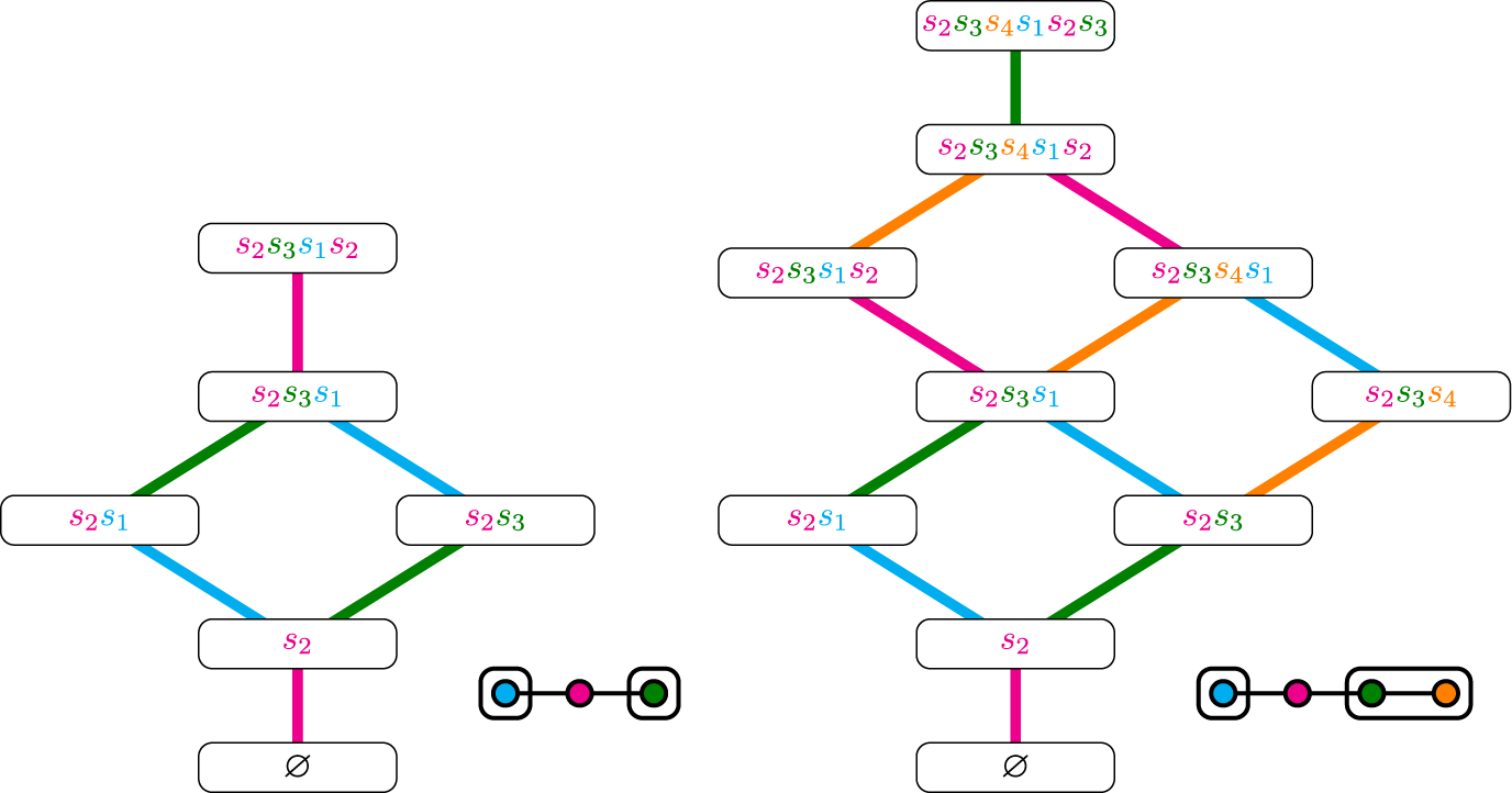
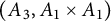
The graph
 $\mathcal {G}_{(W,P)}$
for
$\mathcal {G}_{(W,P)}$
for
 $(W,P)=(A_3,A_1 \times A_1 )$
and
$(W,P)=(A_3,A_1 \times A_1 )$
and
 $(A_4,A_1 \times A_2 )$
respectively. (We haven’t drawn the direction on the edges but all arrows are pointing upward.)
$(A_4,A_1 \times A_2 )$
respectively. (We haven’t drawn the direction on the edges but all arrows are pointing upward.)
The graph
 $\mathcal {G}_{(W,P)}$
for types
$\mathcal {G}_{(W,P)}$
for types
 $(W,P)=(D_5, D_4)$
and
$(W,P)=(D_5, D_4)$
and
 $(B_4 , B_3)$
. The general case
$(B_4 , B_3)$
. The general case
 $(D_{n+1},D_n)$
and
$(D_{n+1},D_n)$
and
 $(B_n,B_{n-1})$
is no more difficult (see [Reference Bowman, De Visscher, Hazi and NortonBDHN, Section 1]) – merely extend the top and bottom vertical chains of the graph.
$(B_n,B_{n-1})$
is no more difficult (see [Reference Bowman, De Visscher, Hazi and NortonBDHN, Section 1]) – merely extend the top and bottom vertical chains of the graph.

The identity element
 $1 \in W$
is the minimal coset representative of the identity coset P, and for convenience, we will denote it by
$1 \in W$
is the minimal coset representative of the identity coset P, and for convenience, we will denote it by
 $\varnothing $
instead (the empty word in the generators).
$\varnothing $
instead (the empty word in the generators).
We now define
 $\widehat {\mathcal {G}}_{(W,P)}$
to be the directed graph having the same set of vertices as
$\widehat {\mathcal {G}}_{(W,P)}$
to be the directed graph having the same set of vertices as
 $\mathcal {G}_{(W,P)}$
but replacing each edge in
$\mathcal {G}_{(W,P)}$
but replacing each edge in
 $\mathcal {G}_{(W,P)}$
between
$\mathcal {G}_{(W,P)}$
between
 $\lambda $
and
$\lambda $
and
 $\lambda s_i$
by four directed edges
$\lambda s_i$
by four directed edges
 $$\begin{align*}\lambda \xrightarrow{ \ s_i \ }\lambda , \quad \lambda s_i \xrightarrow{ \ s_i \ }\lambda s_i, \quad \lambda \xrightarrow{ \ s_i \ }\lambda s_i , \quad \lambda s_i \xrightarrow{ \ s_i \ }\lambda \end{align*}$$
and, in order to keep the notation to a minimum, we will simply label the edge by the subscript of the reflection (not the reflection itself). We assign a degree to each edge in
 $\widehat {\mathcal {G}}_{(W,P)}$
by setting
$\widehat {\mathcal {G}}_{(W,P)}$
by setting
 $$\begin{align*}\mathrm{deg}(\lambda \xrightarrow{ \ i \ } \lambda s_i) = \mathrm{deg}(\lambda s_i \xrightarrow{ \ i \ } \lambda) = 0 \qquad \mathrm{deg}(\lambda \xrightarrow{ \ i \ } \lambda) = \left\{ \begin{array}{ll} 1 & \text{if } \lambda s_i> \lambda\\ -1 & \text{if } \lambda s_i < \lambda.\end{array}\right.\end{align*}$$
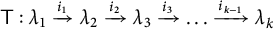
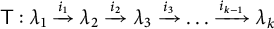
Given a path (or “Bruhat stroll”) on
 $\widehat {\mathcal {G}}_{(W,P)}$
 $$\begin{align*}\mathsf{T} \, : \, \lambda_1 \xrightarrow{i_1} \lambda_2 \xrightarrow{i_2} \lambda_3 \xrightarrow{i_3} \ldots \xrightarrow{i_{k-1}} \lambda_k,\end{align*}$$
we say that the degree
 $\mathrm {deg}(\mathsf {T})$
is the sum of the degrees of each edge in
$\mathrm {deg}(\mathsf {T})$
is the sum of the degrees of each edge in
 $\mathsf {T}$
. (The degree is also sometimes known as the “Deodhar defect”.) We also define the weight of
$\mathsf {T}$
. (The degree is also sometimes known as the “Deodhar defect”.) We also define the weight of
 $\mathsf {T}$
, denoted by
$\mathsf {T}$
, denoted by
 $\omega (\mathsf {T})$
to be the expression
$\omega (\mathsf {T})$
to be the expression
 $$\begin{align*}\omega(\mathsf{T}) := {s_{i_1}s_{i_2}s_{i_3} \ldots s_{i_{k-1}}}.\end{align*}$$
We write
 $\mathrm {Path}_{(W,P)}$
for the set of all paths on
$\mathrm {Path}_{(W,P)}$
for the set of all paths on
 $\widehat {\mathcal {G}}_{(W,P)}$
. For
$\widehat {\mathcal {G}}_{(W,P)}$
. For
 $\lambda , \nu \in {^PW}$
, we let
$\lambda , \nu \in {^PW}$
, we let
 $\mathrm {Path} (\lambda \to \nu )$
denote the set of all paths in
$\mathrm {Path} (\lambda \to \nu )$
denote the set of all paths in
 $\mathrm {Path}_{(W,P)}$
beginning at
$\mathrm {Path}_{(W,P)}$
beginning at
 $\lambda $
and ending at
$\lambda $
and ending at
 $\nu $
. When
$\nu $
. When
 $\lambda = \varnothing ,$
we set
$\lambda = \varnothing ,$
we set
 $\mathrm {Path} ( \nu ):=\mathrm {Path} (\varnothing \to \nu )$
. Let
$\mathrm {Path} ( \nu ):=\mathrm {Path} (\varnothing \to \nu )$
. Let
 $\underline {w}$
be an expression in the generators
$\underline {w}$
be an expression in the generators
 $S_W$
. We set
$S_W$
. We set
 $\mathrm {Path} (\lambda \to \nu ,{\underline {w}})$
to be the set of paths
$\mathrm {Path} (\lambda \to \nu ,{\underline {w}})$
to be the set of paths
 $\mathsf {T}\in \mathrm {Path}(\lambda \to \nu )$
with
$\mathsf {T}\in \mathrm {Path}(\lambda \to \nu )$
with
 $\omega (\mathsf {T}) = \underline {w}$
. When
$\omega (\mathsf {T}) = \underline {w}$
. When
 $\lambda = \varnothing ,$
we set
$\lambda = \varnothing ,$
we set
 $\mathrm {Path}(\nu , \underline {w}) := \mathrm {Path}(\varnothing \to \nu , \underline {w})$
.
$\mathrm {Path}(\nu , \underline {w}) := \mathrm {Path}(\varnothing \to \nu , \underline {w})$
.
Throughout the paper, we fix one reduced expression
 $\underline {\mu }$
for each
$\underline {\mu }$
for each
 $\mu \in {^PW}$
. The set of paths
$\mu \in {^PW}$
. The set of paths
 $\mathrm {Path}(\lambda , \underline {\mu })$
for
$\mathrm {Path}(\lambda , \underline {\mu })$
for
 $\lambda , \mu \in {^PW}$
will play a crucial role. Examples of such paths are given in Figure 4. We will see in particular that, for Hermitian symmetric pairs, the set
$\lambda , \mu \in {^PW}$
will play a crucial role. Examples of such paths are given in Figure 4. We will see in particular that, for Hermitian symmetric pairs, the set
 $ \mathrm {Path} (\lambda ,\underline {\mu })$
consists of either 0 or 1 elements.
$ \mathrm {Path} (\lambda ,\underline {\mu })$
consists of either 0 or 1 elements.
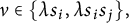
On the left we depict the unique path in
 $\mathrm {Path}(\alpha , \underline {\alpha })$
corresponding with a choice of reduced word
$\mathrm {Path}(\alpha , \underline {\alpha })$
corresponding with a choice of reduced word
 $\underline {\alpha }$
and on the right we depict the unique element of
$\underline {\alpha }$
and on the right we depict the unique element of
 $\mathrm {Path}(\beta ,\underline {\alpha })$
for
$\mathrm {Path}(\beta ,\underline {\alpha })$
for ![]() and
and ![]() . These are paths on
. These are paths on
 $\widehat {\mathcal {G}}_{ {(A_4, A_1\times A_2)} } $
(also known as “Bruhat strolls”) but we depict only the edges in
$\widehat {\mathcal {G}}_{ {(A_4, A_1\times A_2)} } $
(also known as “Bruhat strolls”) but we depict only the edges in
 ${\mathcal {G}}_{ {(A_4,A_1\times A_2)} }$
(for readability).
${\mathcal {G}}_{ {(A_4,A_1\times A_2)} }$
(for readability).

The following path theoretic definition of Kazhdan–Lusztig polynomials was for a long time talked about implicitly in the literature, see for example [Reference DeodharDeo90] (in particular Proposition 3.5 and Section 4, and also Section 5 for the parabolic setting). It is explicitly proven to be equivalent to the classical definition of these polynomials in [Reference SoergelSoe97, Proposition 3.3].
Definition 2.1 Let
 $\lambda ,\mu \in {{^P}W}$
. We set
$\lambda ,\mu \in {{^P}W}$
. We set
 $b_{\lambda ,\underline {\lambda }}(q)=1=n_{\lambda ,\lambda }(q)$
. For
$b_{\lambda ,\underline {\lambda }}(q)=1=n_{\lambda ,\lambda }(q)$
. For
 $\lambda \neq \mu $
, we recursively define the polynomials
$\lambda \neq \mu $
, we recursively define the polynomials
 $$\begin{align*}b_{\lambda,\underline{\mu}}(q)\in {\mathbb Z} [q+q^{-1}] \qquad n_{\lambda,\mu}(q)\in q{\mathbb Z} [q] \end{align*}$$
by induction on the Bruhat order
 $\leq $
as follows
$\leq $
as follows
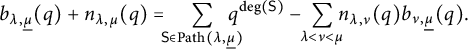 $$ \begin{align} b_{\lambda,\underline{\mu}}(q) +n_{\lambda,\mu}(q) = \!\!\! \sum_{\mathsf{S} \in \mathrm{Path}(\lambda,\underline{\mu})}\!\!\!\!\!\! q^{\deg(\mathsf{S})} - \!\!\sum_{ \begin{subarray}c \lambda < \nu < \mu\end{subarray} } \!\!\! n_{\lambda,\nu}(q) b_{\nu,\underline{\mu}}(q). \end{align} $$
The polynomials
 $n_{\lambda ,\mu }(q)$
are called the anti-spherical Kazhdan–Lusztig polynomials associated to
$n_{\lambda ,\mu }(q)$
are called the anti-spherical Kazhdan–Lusztig polynomials associated to
 $\lambda ,\mu \in {^PW}$
.
$\lambda ,\mu \in {^PW}$
.
We can reformulate the above in terms of matrix multiplication. We define the matrix of light leaves polynomials
 $$\begin{align*}\Delta^{(W,P)}:=( \Delta_{\lambda,\underline{\mu}}(q))_{\lambda,\mu\in {{^P}W}} \qquad \qquad \Delta_{\lambda,\underline{\mu}}(q)=\sum_{\mathsf{S} \in \mathrm{Path}(\lambda,\underline{\mu})}\!\!\!\!\!\! q^{\deg(\mathsf{S})} \end{align*}$$
to be the (square) lower uni-triangular matrix whose entries record the degrees of paths in
 $\mathrm {Path}(\lambda ,\underline {\mu })$
. This matrix can be factorized uniquely as a product
$\mathrm {Path}(\lambda ,\underline {\mu })$
. This matrix can be factorized uniquely as a product
 $\Delta ^{(W,P)}= N^{(W,P)} \times B^{(W,P)}$
of lower uni-triangular matrices
$\Delta ^{(W,P)}= N^{(W,P)} \times B^{(W,P)}$
of lower uni-triangular matrices
 $$\begin{align*}N^{(W,P)}:=(n_{\lambda,\nu}(q))_{\lambda,\mu\in {{^P}W}} \qquad B^{(W,P)}:=(b_{\nu,\underline{\mu}}(q))_{\nu,\mu\in {{^P}W},} \end{align*}$$
such that
 $n_{\lambda ,\nu }(q)\in q{\mathbb Z}[q]$
for
$n_{\lambda ,\nu }(q)\in q{\mathbb Z}[q]$
for
 $\lambda \neq \nu $
and
$\lambda \neq \nu $
and
 $b_{\nu ,\underline {\mu }}(q)\in {\mathbb Z}[q+q^{-1}]$
.
$b_{\nu ,\underline {\mu }}(q)\in {\mathbb Z}[q+q^{-1}]$
.
Example 2.2 The matrix
 $\Delta $
in type
$\Delta $
in type
 $(A_3,A_1\times A_1)$
is depicted below.
$(A_3,A_1\times A_1)$
is depicted below.
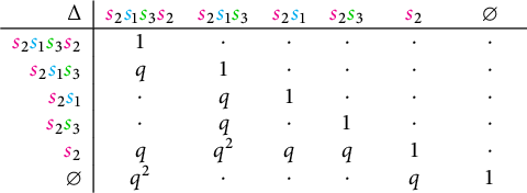
The factorization of this matrix is trivial, with
 $N=\Delta $
and
$N=\Delta $
and
 $B=\mathrm {Id}_{6\times 6}$
the identity matrix.
$B=\mathrm {Id}_{6\times 6}$
the identity matrix.
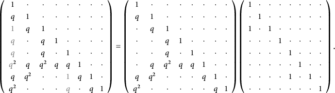
Example 2.3 For
 $(C_3,A_2)$
the factorization
$(C_3,A_2)$
the factorization
 $\Delta = N\times B$
is given below. The rows of the matrix can be taken to be ordered with respect to any total refinement of the Bruhat order (there are two such total orders), see Figure 9 for the corresponding graph
$\Delta = N\times B$
is given below. The rows of the matrix can be taken to be ordered with respect to any total refinement of the Bruhat order (there are two such total orders), see Figure 9 for the corresponding graph
 $\mathcal {G}_{(W,P)}$
.
$\mathcal {G}_{(W,P)}$
.
Example 2.4 The matrices
 $\Delta $
for exceptional types of Hermitian symmetric pairs are given in Section 4. Again, we have that B is the identity matrix in these cases.
$\Delta $
for exceptional types of Hermitian symmetric pairs are given in Section 4. Again, we have that B is the identity matrix in these cases.
The paths
 $\mathsf {S} \in \mathrm {Path}(\lambda ,\underline {\mu })$
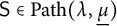
enumerate a “light leaf basis” of the Hecke category. We refer to [Reference Bowman, De Visscher, Hazi and NortonBDHN] for an algorithmic construction of these basis elements in the language of this paper, see also [Reference Libedinsky and WilliamsonLW]. We are now able to restate Libedinsky–Williamson’s goal (from the introduction) more precisely using the language of paths. They ask if it is possible to produce (via a closed combinatorial algorithm) a set
$\mathsf {S} \in \mathrm {Path}(\lambda ,\underline {\mu })$
enumerate a “light leaf basis” of the Hecke category. We refer to [Reference Bowman, De Visscher, Hazi and NortonBDHN] for an algorithmic construction of these basis elements in the language of this paper, see also [Reference Libedinsky and WilliamsonLW]. We are now able to restate Libedinsky–Williamson’s goal (from the introduction) more precisely using the language of paths. They ask if it is possible to produce (via a closed combinatorial algorithm) a set
 $\mathrm {NPath} (\lambda ,\underline {\nu }) \subseteq \mathrm {Path} (\lambda ,\underline {\nu })$
and a canonical basis for a space
$\mathrm {NPath} (\lambda ,\underline {\nu }) \subseteq \mathrm {Path} (\lambda ,\underline {\nu })$
and a canonical basis for a space
 $$\begin{align*}\bigoplus_{\mathsf{s} \in \mathrm{NPath} (\lambda,\underline{\nu})} \mathbb{R}\mathsf{s} \xrightarrow{ \sim } \mathbb N_{\lambda,\nu} \end{align*}$$
so that, upon taking graded dimensions, we get
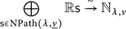
 $$\begin{align*}n_{\lambda,\nu} = \sum _{\mathsf{s} \in \mathrm{NPath} (\lambda,\underline{\nu})} q^{\deg(\mathsf{s})}. \end{align*}$$
In this paper, we answer this question for
 $(W,P)$
a Hermitian symmetric pair (see Figure 1 for a list of such pairs). In fact, we go further and produce closed combinatorial descriptions of canonical bases for spaces
$(W,P)$
a Hermitian symmetric pair (see Figure 1 for a list of such pairs). In fact, we go further and produce closed combinatorial descriptions of canonical bases for spaces
 $$\begin{align*}\bigoplus_{\mathsf{s} \in \mathrm{NPath} (\lambda,\underline{\nu})} \mathbb{R}\mathsf{s} \xrightarrow{ \sim } \mathbb N_{\lambda,\nu} \qquad\qquad \bigoplus_{\mathsf{s} \in \mathrm{BPath} (\lambda,\underline{\nu})} \mathbb{R}\mathsf{s} \xrightarrow{ \sim } \mathbb B_{\lambda,\underline{\nu}} \end{align*}$$
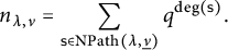
so that, upon taking graded dimensions, we get
 $$\begin{align*}n_{\lambda,\nu} = \sum _{\mathsf{s} \in \mathrm{NPath} (\lambda,\underline{\nu})} q^{\deg(\mathsf{s})} \qquad \qquad b_{\nu,\underline{\mu}} = \sum _{\mathsf{s} \in \mathrm{BPath} (\nu,\underline{\mu})} q^{\deg(\mathsf{s})} \end{align*}$$
for subsets
 $\mathrm {NPath} (\lambda ,\underline {\nu }) \subseteq \mathrm {Path} (\lambda ,\underline {\nu })$
and
$\mathrm {NPath} (\lambda ,\underline {\nu }) \subseteq \mathrm {Path} (\lambda ,\underline {\nu })$
and
 $ \mathrm {BPath} (\nu ,\underline {\mu }) \subseteq \mathrm {Path} (\nu ,\underline {\mu })$
.
$ \mathrm {BPath} (\nu ,\underline {\mu }) \subseteq \mathrm {Path} (\nu ,\underline {\mu })$
.
We note further that, for Hermitian symmetric pairs, the subsets
 $\mathrm {NPath} (\lambda ,\underline {\nu })$
and
$\mathrm {NPath} (\lambda ,\underline {\nu })$
and
 $\mathrm {BPath} (\nu ,\underline {\mu })$
are independent of the choice of reduced expressions for
$\mathrm {BPath} (\nu ,\underline {\mu })$
are independent of the choice of reduced expressions for
 $\mu $
and
$\mu $
and
 $\nu $
. This follows from the fact that the elements of
$\nu $
. This follows from the fact that the elements of
 ${^PW}$
are fully commutative (see Section 3.1 below).
${^PW}$
are fully commutative (see Section 3.1 below).
3 The oriented Temperley–Lieb algebras
We will assume from now on that
 $(W,P)$
is a Hermitian symmetric pair, that is it is one of the following infinite families
$(W,P)$
is a Hermitian symmetric pair, that is it is one of the following infinite families
 $(A_n , A_{k-1} \times A_{n-k} )$
with
$(A_n , A_{k-1} \times A_{n-k} )$
with
 $1 \leq k \leq n$
,
$1 \leq k \leq n$
,
 $(D_n , A_{n-1} )$
,
$(D_n , A_{n-1} )$
,
 $(D_n , D_{n-1} )$
,
$(D_n , D_{n-1} )$
,
 $(B_n , B_{n-1} )$
,
$(B_n , B_{n-1} )$
,
 $(C_n , A_{n-1} )$
for
$(C_n , A_{n-1} )$
for
 $n\geq 2$
or is one of the exceptional cases
$n\geq 2$
or is one of the exceptional cases
 $(E_6,D_5)$
,
$(E_6,D_5)$
,
 $(E_7,E_6)$
. The corresponding Coxeter graphs of these pairs are recorded in Figure 1.
$(E_7,E_6)$
. The corresponding Coxeter graphs of these pairs are recorded in Figure 1.
3.1 The oriented Temperley–Lieb algebras and strong full commutativity
For
 $\underline {w}, \underline {w}'$
two expressions in the generators
$\underline {w}, \underline {w}'$
two expressions in the generators
 $s_i\in S_W$
, we say that
$s_i\in S_W$
, we say that
 $\underline {w'}$
is a subword of
$\underline {w'}$
is a subword of
 $\underline {w}$
if there are expressions
$\underline {w}$
if there are expressions
 $\underline {u}$
and
$\underline {u}$
and
 $\underline {v}$
such that
$\underline {v}$
such that
 $\underline {w} = \underline {u} \, \underline {w'} \,\underline {v}$
. One of the crucial property of Hermitian symmetric pairs for this paper is that the elements of
$\underline {w} = \underline {u} \, \underline {w'} \,\underline {v}$
. One of the crucial property of Hermitian symmetric pairs for this paper is that the elements of
 $^PW$
are fully commutative (as defined by Stembridge [Reference StembridgeSte96, Introduction]). We recall that an element
$^PW$
are fully commutative (as defined by Stembridge [Reference StembridgeSte96, Introduction]). We recall that an element
 $w\in W$
is called fully commutative if and only if any two reduced expression of w are related by applying only the commutation relations in W. Equivalently, no reduced expressions of w contains
$w\in W$
is called fully commutative if and only if any two reduced expression of w are related by applying only the commutation relations in W. Equivalently, no reduced expressions of w contains
 $s_is_js_i$
as a subword for
$s_is_js_i$
as a subword for
 $m_{i,j}=3$
or
$m_{i,j}=3$
or
 $s_is_js_is_j$
as a subword for
$s_is_js_is_j$
as a subword for
 $m_{i,j}=4$
. In fact, the elements of
$m_{i,j}=4$
. In fact, the elements of
 ${^PW}$
satisfy the following slightly stronger property.
${^PW}$
satisfy the following slightly stronger property.
Definition 3.1 We say that an element
 $w\in W$
is strongly fully commutative if no reduced expression of w contains
$w\in W$
is strongly fully commutative if no reduced expression of w contains
 $s_is_js_i$
as a subword for any
$s_is_js_i$
as a subword for any
 $s_i,s_j\in S_W$
with either
$s_i,s_j\in S_W$
with either
 $m_{i,j}=3$
or
$m_{i,j}=3$
or
 $m_{i,j}=4$
when
$m_{i,j}=4$
when
 $\alpha _i$
is a short root. We denote by
$\alpha _i$
is a short root. We denote by
 $W_{sfc}$
the set of all strongly fully commutative elements of W.
$W_{sfc}$
the set of all strongly fully commutative elements of W.
Lemma 3.2 Let
 $(W,P)$
be a Hermitian symmetric pair. Then every element of
$(W,P)$
be a Hermitian symmetric pair. Then every element of
 ${^PW}$
is strongly fully commutative.
${^PW}$
is strongly fully commutative.
Proof This is well-known and can be seen for example from the explicit description of the elements of
 $^PW$
in terms of tilings given in [Reference Enright, Hunziker and PruettEHP14, Appendix: Diagrams of Hermitian types].
$^PW$
in terms of tilings given in [Reference Enright, Hunziker and PruettEHP14, Appendix: Diagrams of Hermitian types].
Definition 3.3 Let
 $(W,P)$
be a Hermitian symmetric pair. The oriented Temperley–Lieb algebra of type
$(W,P)$
be a Hermitian symmetric pair. The oriented Temperley–Lieb algebra of type
 $(W,P)$
,
$(W,P)$
,
 $\mathrm {TL}_{(W,P)}(q)$
, is defined to be the unital associative
$\mathrm {TL}_{(W,P)}(q)$
, is defined to be the unital associative
 $\mathbb {Z}[q,q^{-1}]$
-algebra generated by elements
$\mathbb {Z}[q,q^{-1}]$
-algebra generated by elements
 $$\begin{align*}\{\mathsf{1}_\lambda \mid \lambda \in {^PW}\} \cup \{ E_i \mid s_i\in S_W\} \end{align*}$$
subject to the following relations. The idempotent relations,
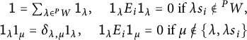 $$ \begin{align} \mathsf{1}= \textstyle\sum_{\lambda\in {^PW}} \mathsf{1}_\lambda, \quad \mathsf{1}_\lambda E_i \mathsf{1}_\lambda= 0 \text{ if } \lambda s_i \notin {^PW}, \nonumber\\ \mathsf{1}_\lambda 1_\mu =\delta_{\lambda,\mu}1_\lambda , \quad \mathsf{1}_\lambda E_i \mathsf{1}_\mu= 0 \text{ if } \mu \not \in \{\lambda,\lambda s_i \} \end{align} $$
for all
 $\lambda , \mu \in {^PW}$
. For all
$\lambda , \mu \in {^PW}$
. For all
 $s_i\in S_W$
, any
$s_i\in S_W$
, any
 $\lambda \in {^PW}$
with
$\lambda \in {^PW}$
with
 $\lambda s_i \in {^PW}$
and
$\lambda s_i \in {^PW}$
and
 $\mu , \nu \in \{\lambda , \lambda s_i\}$
we have
$\mu , \nu \in \{\lambda , \lambda s_i\}$
we have
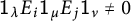
 $$ \begin{align} \mathsf{1}_\mu E_{ i} \mathsf{1}_\lambda E_{ i} \mathsf{1}_\nu = q^{ \ell(\lambda s_i)-\ell(\lambda)} \mathsf{1}_\mu E_i \mathsf{1}_\nu. \end{align} $$
If
 $m_{i,j}=2$
or
$m_{i,j}=2$
or
 $3$
, then
$3$
, then
 $$ \begin{align} E_i E_j=E_jE_i, \qquad\quad E_iE_jE_i = E_i, \end{align} $$
respectively. If
 $m_{i,j}=4$
and
$m_{i,j}=4$
and
 $\alpha _i$
is a short root then we have that
$\alpha _i$
is a short root then we have that
 $$ \begin{align} \mathsf{1}_\mu E_i \mathsf{1}_\lambda E_j \mathsf{1}_\lambda E_i \mathsf{1}_\nu = \mathsf{1}_\mu E_i \mathsf{1}_\nu, \end{align} $$
for any
 $\lambda \in {^PW}$
with
$\lambda \in {^PW}$
with
 $\lambda s_i, \lambda s_j\in {^PW}$
and
$\lambda s_i, \lambda s_j\in {^PW}$
and
 $\mu , \nu \in \{\lambda , \lambda s_i\}$
.
$\mu , \nu \in \{\lambda , \lambda s_i\}$
.
Remark 3.4 It follows from the relations (3.1) that
 $\mathrm {TL}_{(W,P)}(q)$
is generated by the elements
$\mathrm {TL}_{(W,P)}(q)$
is generated by the elements
 $\mathsf {1}_\lambda $
for
$\mathsf {1}_\lambda $
for
 $\lambda \in {^PW}$
and
$\lambda \in {^PW}$
and
 $\mathsf {1}_\lambda E_i \mathsf {1}_\mu $
for all
$\mathsf {1}_\lambda E_i \mathsf {1}_\mu $
for all
 $\lambda \in {^PW}$
with
$\lambda \in {^PW}$
with
 $\lambda s_i\in {^PW}$
and
$\lambda s_i\in {^PW}$
and
 $\mu \in \{ \lambda , \lambda s_i\}$
.
$\mu \in \{ \lambda , \lambda s_i\}$
.
Remark 3.5 Note that for
 $m_{i,j}=2$
we have
$m_{i,j}=2$
we have
 $\mathsf {1}_\lambda E_i \mathsf {1}_\mu E_j \mathsf {1}_\nu \neq 0$
if and only if
$\mathsf {1}_\lambda E_i \mathsf {1}_\mu E_j \mathsf {1}_\nu \neq 0$
if and only if
 $\lambda , \lambda s_i, \lambda s_j\in {^PW}$
and either
$\lambda , \lambda s_i, \lambda s_j\in {^PW}$
and either
 $\mu = \lambda $
and
$\mu = \lambda $
and
 $\nu \in \{\lambda , \lambda s_j\}$
, or
$\nu \in \{\lambda , \lambda s_j\}$
, or
 $\mu = \lambda s_i$
and
$\mu = \lambda s_i$
and
 $\nu \in \{ \lambda s_i, \lambda s_i s_j\}$
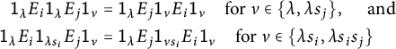
. So we have that the first relation in (3.3) is equivalent to
$\nu \in \{ \lambda s_i, \lambda s_i s_j\}$
. So we have that the first relation in (3.3) is equivalent to
 $$\begin{align*}\mathsf{1}_\lambda E_i \mathsf{1}_\lambda E_j \mathsf{1}_\nu = \mathsf{1}_\lambda E_j \mathsf{1}_\nu E_i \mathsf{1}_\nu, \quad \text{ and } \quad \mathsf{1}_\lambda E_i \mathsf{1}_{\lambda s_i} E_j \mathsf{1}_\nu = \mathsf{1}_\lambda E_j \mathsf{1}_{\nu s_i} E_i \mathsf{1}_\nu\end{align*}$$
for
 $\nu \in \{ \lambda , \lambda s_j\}$
and
$\nu \in \{ \lambda , \lambda s_j\}$
and
 $\nu \in \{ \lambda s_i, \lambda s_is_j\},$
respectively, and every
$\nu \in \{ \lambda s_i, \lambda s_is_j\},$
respectively, and every
 $\lambda \in {^PW}$
.
$\lambda \in {^PW}$
.
Remark 3.6 Note that for
 $m_{i,j}=3$
, using Lemma 3.2, we have
$m_{i,j}=3$
, using Lemma 3.2, we have
 $ E_i \mathsf {1}_\mu E_j \mathsf {1}_\nu E_i \neq 0$
implies
$ E_i \mathsf {1}_\mu E_j \mathsf {1}_\nu E_i \neq 0$
implies
 $\nu = \mu $
and
$\nu = \mu $
and
 $\mu s_i, \mu s_j\in {^PW}$
. Now the second relation in (3.3) is equivalent to
$\mu s_i, \mu s_j\in {^PW}$
. Now the second relation in (3.3) is equivalent to
 $$\begin{align*}\mathsf{1}_\lambda E_i E_j E_i \mathsf{1}_\eta = \mathsf{1}_\lambda E_i \mathsf{1}_\eta\end{align*}$$
for all
 $\lambda , \eta \in {^PW}$
with
$\lambda , \eta \in {^PW}$
with
 $\lambda s_i, \eta s_i\in {^PW}$
. Note that for each such
$\lambda s_i, \eta s_i\in {^PW}$
. Note that for each such
 $\lambda $
, using Lemma 3.2, we have either
$\lambda $
, using Lemma 3.2, we have either
 $\lambda s_j\in {^PW}$
or
$\lambda s_j\in {^PW}$
or
 $\lambda s_i s_j\in {^PW}$
but not both. Thus the second relation in (3.3) is also equivalent to
$\lambda s_i s_j\in {^PW}$
but not both. Thus the second relation in (3.3) is also equivalent to
 $$\begin{align*}\mathsf{1}_\lambda E_i \mathsf{1}_\lambda E_j \mathsf{1}_\lambda E_i \mathsf{1}_\eta = \mathsf{1}_\lambda E_i \mathsf{1}_\eta\end{align*}$$
for all
 $\lambda \in {^PW}$
with
$\lambda \in {^PW}$
with
 $\lambda s_i, \lambda s_j\in {^PW}$
and
$\lambda s_i, \lambda s_j\in {^PW}$
and
 $\eta = \{\lambda , \lambda s_i\}$
, and
$\eta = \{\lambda , \lambda s_i\}$
, and
 $$\begin{align*}\mathsf{1}_\lambda E_i \mathsf{1}_{\lambda s_i} E_j \mathsf{1}_{\lambda s_i} E_i \mathsf{1}_\eta = \mathsf{1}_\lambda E_i \mathsf{1}_\eta\end{align*}$$
for all
 $\lambda \in {^PW}$
with
$\lambda \in {^PW}$
with
 $\lambda s_i, \lambda s_i s_j\in {^PW}$
and
$\lambda s_i, \lambda s_i s_j\in {^PW}$
and
 $\eta = \{\lambda , \lambda s_i\}$
.
$\eta = \{\lambda , \lambda s_i\}$
.
Remark 3.7 Note that for
 $m_{i,j}=4$
with
$m_{i,j}=4$
with
 $\alpha _i$
being a short root, we have
$\alpha _i$
being a short root, we have
 $$\begin{align*}\mathsf{1}_\lambda E_i E_j E_i \mathsf{1}_\mu = \mathsf{1}_\lambda E_i \mathsf{1}_\lambda E_j \mathsf{1}_\lambda E_i \mathsf{1}_\mu + \mathsf{1}_\lambda E_i \mathsf{1}_{\lambda s_i} E_j \mathsf{1}_{\lambda s_i} E_i \mathsf{ 1}_\mu = 2 (\mathsf{1}_\lambda E_i \mathsf{1}_\mu)\end{align*}$$
for
 $\lambda , \lambda s_i, \lambda s_j , \lambda s_i s_j\in {^PW}$
and
$\lambda , \lambda s_i, \lambda s_j , \lambda s_i s_j\in {^PW}$
and
 $\mu \in \{\lambda , \lambda s_i\}$
. This implies that
$\mu \in \{\lambda , \lambda s_i\}$
. This implies that
 $E_iE_jE_i = 2E_i$
and so
$E_iE_jE_i = 2E_i$
and so
 $E_iE_jE_iE_j = 2E_iE_j$
and
$E_iE_jE_iE_j = 2E_iE_j$
and
 $E_jE_iE_jE_i = 2E_jE_i$
.
$E_jE_iE_jE_i = 2E_jE_i$
.
3.2 Path basis and the anti-spherical module
For any path
 $$\begin{align*}{\mathsf{T}} : \lambda_1 \xrightarrow{i_1} \lambda_2 \xrightarrow{i_2} \lambda_3 \xrightarrow{i_3} \ldots \xrightarrow{i_{k-1}} \lambda_k \end{align*}$$
on
 $\widehat {\mathcal {G}}_{(W,P)}$
, we write
$\widehat {\mathcal {G}}_{(W,P)}$
, we write
 $$\begin{align*}E_{\mathsf{T}} := \mathsf{1}_{\lambda_1} E_{i_1} \mathsf{1}_{\lambda_2} E_{i_2} \mathsf{1}_{\lambda_3} \ldots \mathsf{1}_{\lambda_{k-1}} E_{i_{k-1}} \mathsf{1}_{\lambda_{i_k}} \end{align*}$$
to be the corresponding element in
 $\mathrm {TL}_{(W,P)}(q)$
.
$\mathrm {TL}_{(W,P)}(q)$
.
Recall that we denote by
 $W_{sfc}$
the set of all strongly fully commutative elements of W. We now fix one reduced expression
$W_{sfc}$
the set of all strongly fully commutative elements of W. We now fix one reduced expression
 $\underline {w}$
for each
$\underline {w}$
for each
 $w\in W_{sfc}$
.
$w\in W_{sfc}$
.
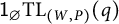
Theorem 3.8 The algebra
 $\mathrm {TL}_{(W,P)}(q)$
has a
$\mathrm {TL}_{(W,P)}(q)$
has a
 $\mathbb {Z}[q,q^{-1}]$
-basis given by the set
$\mathbb {Z}[q,q^{-1}]$
-basis given by the set
 $$\begin{align*}\{ E_{\mathsf{T}} \, : \, \mathsf{T}\in\mathrm{Path}_{(W,P)} \,\, \text{with} \,\, \omega(\mathsf{T})=\underline{w} \,\, \text{for some } w\in W_{sfc}\}.\end{align*}$$
Proof It is clear from relations (3.1) that
 $$\begin{align*}\mathsf{1}_{\lambda_1} E_{i_1} \mathsf{1}_{\lambda_2} E_{i_2} \mathsf{1}_{\lambda_3} \ldots \mathsf{1}_{\lambda_{k-1}} E_{i_{k-1}} \mathsf{1}_{\lambda_{k}} \neq 0 \end{align*}$$
implies that
 $$\begin{align*}\mathsf{T} : \lambda_1 \xrightarrow{i_1} \lambda_2 \xrightarrow{i_2} \lambda_3 \xrightarrow{i_3} \ldots \xrightarrow{i_{k-1}} \lambda_k \end{align*}$$
is a path on
 $\widehat {\mathcal {G}}_{(W,P)}$
. Thus we have that
$\widehat {\mathcal {G}}_{(W,P)}$
. Thus we have that
 $\mathrm {TL}_{(W,P)}(q)$
is spanned by elements of the form
$\mathrm {TL}_{(W,P)}(q)$
is spanned by elements of the form
 $E_{\mathsf {T}}$
where
$E_{\mathsf {T}}$
where
 $\mathsf {T}\in \mathrm {Path}_{(W,P)}$
. Now it follows from relations (3.2)–(3.4) that any such
$\mathsf {T}\in \mathrm {Path}_{(W,P)}$
. Now it follows from relations (3.2)–(3.4) that any such
 $E_{\mathsf {T}} = q^x E_{\mathsf {S}}$
for some
$E_{\mathsf {T}} = q^x E_{\mathsf {S}}$
for some
 $x\in \mathbb {Z}$
and some path
$x\in \mathbb {Z}$
and some path
 $\mathsf {S}$
such that
$\mathsf {S}$
such that
 $\omega (\mathsf {S})=\underline {w}$
for some
$\omega (\mathsf {S})=\underline {w}$
for some
 $w\in W_{sfc}$
. Set
$w\in W_{sfc}$
. Set
 $\mathrm { Path}_{(W,P)}^{sfc}$
to be the set of all
$\mathrm { Path}_{(W,P)}^{sfc}$
to be the set of all
 $\mathsf {T} \in \mathrm {Path}_{(W,P)}$
such that
$\mathsf {T} \in \mathrm {Path}_{(W,P)}$
such that
 $\omega (\mathsf {T}) = \underline {w}$
for some
$\omega (\mathsf {T}) = \underline {w}$
for some
 $w\in W_{sfc}$
. It remains to show that the set
$w\in W_{sfc}$
. It remains to show that the set
 $\{ E_{\mathsf {T}} \, : \, \omega (\mathsf {T}) \in \mathrm {Path}_{(W,P)}^{sfc} \}$
is linearly independent. We do this by constructing a formal
$\{ E_{\mathsf {T}} \, : \, \omega (\mathsf {T}) \in \mathrm {Path}_{(W,P)}^{sfc} \}$
is linearly independent. We do this by constructing a formal
 $\mathrm {TL}_{(W,P)}(q)$
-module M with
$\mathrm {TL}_{(W,P)}(q)$
-module M with
 $\mathbb {Z}[q,q^{-1}]$
-basis labeled by
$\mathbb {Z}[q,q^{-1}]$
-basis labeled by
 $[\mathsf {T}]$
for
$[\mathsf {T}]$
for
 $\mathsf {T}\in \mathrm {{Path}}_{(W,P)}^{sfc}$
. To define the action on this module, we will need to ‘reduce’ any path on
$\mathsf {T}\in \mathrm {{Path}}_{(W,P)}^{sfc}$
. To define the action on this module, we will need to ‘reduce’ any path on
 ${\widehat {\mathcal {G}}_{(W,P)}}$
using the following local operations.
${\widehat {\mathcal {G}}_{(W,P)}}$
using the following local operations.
-
• If
 $m_{ij}=2$
then for
$\nu \in \{\lambda , \lambda s_j\},$
we set and for
$$\begin{align*}[\lambda \xrightarrow{i} \lambda \xrightarrow{j} \nu ] \qquad \implies \qquad [ \lambda \xrightarrow{j} \nu \xrightarrow{i} \lambda]\end{align*}$$
$\nu \in \{\lambda s_i, \lambda s_i s_j\}$
we set
$$\begin{align*}[\lambda \xrightarrow{i} \lambda s_i \xrightarrow{j} \nu] \qquad \implies \qquad [\lambda \xrightarrow{j} \nu s_i \xrightarrow{i} \nu].\end{align*}$$
$m_{ij}=2$
then for
$\nu \in \{\lambda , \lambda s_j\},$
we set and for
$$\begin{align*}[\lambda \xrightarrow{i} \lambda \xrightarrow{j} \nu ] \qquad \implies \qquad [ \lambda \xrightarrow{j} \nu \xrightarrow{i} \lambda]\end{align*}$$
$\nu \in \{\lambda s_i, \lambda s_i s_j\}$
we set
$$\begin{align*}[\lambda \xrightarrow{i} \lambda s_i \xrightarrow{j} \nu] \qquad \implies \qquad [\lambda \xrightarrow{j} \nu s_i \xrightarrow{i} \nu].\end{align*}$$
-
• If
$m_{ij}=3$
or
$m_{ij} = 4$
and
$\alpha _i$
is a short root then for
$\eta \in \{\lambda , \lambda s_i\},$
we set and
$$\begin{align*}[ \lambda \xrightarrow{i} \lambda \xrightarrow{j} \lambda \xrightarrow{i} \eta] \qquad \implies \qquad [\lambda \xrightarrow{i} \eta]\end{align*}$$
$$\begin{align*}[ \lambda \xrightarrow{i} \lambda s_i \xrightarrow{j} \lambda s_i \xrightarrow{i} \eta] \qquad \implies \qquad [\lambda \xrightarrow{i} \eta].\end{align*}$$
-
• For for
$\mu , \nu \in \{\lambda , \lambda s_i\}$
, we set
$$\begin{align*}[\mu \xrightarrow{i} \lambda \xrightarrow{i} \nu ] \qquad \implies \qquad q^{\ell (\lambda s_i) - \ell (\lambda)} [\mu \xrightarrow{i} \nu].\end{align*}$$


(Note that these follow exactly the relations given in Definition 3.3, see also Remark 3.5, Remark 3.6 and Remark 3.7.) It is clear that starting with any path
 $\mathsf {T}\in \mathrm {Path}_{(W,P)}$
, applying these operations repeatedly, we obtain a uniquely defined power
$\mathsf {T}\in \mathrm {Path}_{(W,P)}$
, applying these operations repeatedly, we obtain a uniquely defined power
 $q^{x(\mathsf {T})}$
and a unique path
$q^{x(\mathsf {T})}$
and a unique path
 $\mathrm {rex}(\mathsf {T})\in \mathrm { {Path}}_{{(W,P)}}^{sfc}$
. Now, for any
$\mathrm {rex}(\mathsf {T})\in \mathrm { {Path}}_{{(W,P)}}^{sfc}$
. Now, for any
 $\mathsf {T} \in \mathrm {{Path}}_{{(W,P)}}^{sfc}$
with
$\mathsf {T} \in \mathrm {{Path}}_{{(W,P)}}^{sfc}$
with
 $$\begin{align*}\mathsf{T} : \lambda_1 \xrightarrow{i_1} \lambda_2 \xrightarrow{i_2} \lambda_3 \xrightarrow{i_3} \ldots \xrightarrow{i_{k-1}} \lambda_k =\mu \end{align*}$$
we set
 $$\begin{align*}[\mathsf{T}] \mathsf{1}_\nu = \delta_{\mu \nu} [\mathsf{T}] \quad \text{and} \quad [\mathsf{T}] \mathsf{1}_\mu E_i \mathsf{1}_\nu = q^{x(\mathsf{T}')} [\mathrm{rex}(\mathsf{T}')]\end{align*}$$
for
 $\nu \in \{\mu , \mu s_i\}$
and
$\nu \in \{\mu , \mu s_i\}$
and
 $\mu , \mu s_i\in {^PW}$
, where
$\mu , \mu s_i\in {^PW}$
, where
 $$\begin{align*}\mathsf{T}' = \lambda_1 \xrightarrow{i_1} \lambda_2 \xrightarrow{i_2} \lambda_3 \xrightarrow{i_3} \ldots \xrightarrow{i_{k-1}} \lambda_k = \mu \xrightarrow{i} \nu. \end{align*}$$
As the relations used to reduce the path correspond precisely to the relations defining the oriented Temperley–Lieb algebra, it is clear that this turns M into a
 $\mathrm {TL}_{(W,P)}(q)$
-module.
$\mathrm {TL}_{(W,P)}(q)$
-module.
We are now ready to prove that the set
 $\{ E_{\mathsf {T}} \, : \, \mathsf {T}\in \mathrm {{Path}}_{{(W,P)}}^{sfc}\}$
is linearly independent. Assume that
$\{ E_{\mathsf {T}} \, : \, \mathsf {T}\in \mathrm {{Path}}_{{(W,P)}}^{sfc}\}$
is linearly independent. Assume that
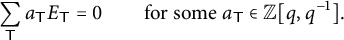 $$\begin{align*}\sum_{\mathsf{T}} a_{\mathsf{T}} E_{\mathsf{T}} = 0 \qquad \text{for some } a_{\mathsf{T}} \in \mathbb{Z}[q,q^{-1}].\end{align*}$$
We need to show that
 $a_{\mathsf {T}} = 0$
for all
$a_{\mathsf {T}} = 0$
for all
 $\mathsf {T}$
. Fix
$\mathsf {T}$
. Fix
 $\lambda \in {^PW}$
and consider the trivial path
$\lambda \in {^PW}$
and consider the trivial path
 $[\lambda ]\in M$
. Then we have
$[\lambda ]\in M$
. Then we have
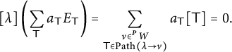 $$\begin{align*}[\lambda] \left( \sum_{\mathsf{T}} a_{\mathsf{T}} E_{\mathsf{T}} \right) = \sum_{ \begin{subarray}{c} {\nu\in {^PW}}\\ \mathsf{T} \in {\mathrm{Path}(\lambda\to\nu)} \end{subarray} } a_{\mathsf{T}} [\mathsf{T}] = 0.\end{align*}$$
As
 $\{[\mathsf {T}] \, : \, \mathsf {T}\in {\mathrm {Path}(\lambda \to \nu )}, \nu \in {^PW} \}$
is linearly independent in M, we deduce that
$\{[\mathsf {T}] \, : \, \mathsf {T}\in {\mathrm {Path}(\lambda \to \nu )}, \nu \in {^PW} \}$
is linearly independent in M, we deduce that
 $a_{\mathsf {T}} = 0$
for all
$a_{\mathsf {T}} = 0$
for all
 $\mathsf {T}\in {\mathrm { Path}(\lambda \to \nu )}$
, all
$\mathsf {T}\in {\mathrm { Path}(\lambda \to \nu )}$
, all
 $\nu \in {^PW}$
. But this holds for all
$\nu \in {^PW}$
. But this holds for all
 $\lambda \in {^PW}$
so we are done.
$\lambda \in {^PW}$
so we are done.
Definition 3.9 We define the anti-spherical
 $\mathrm {TL}_{(W,P)}(q)$
-module to be the right module
$\mathrm {TL}_{(W,P)}(q)$
-module to be the right module
 $ \mathsf {1}_\varnothing \mathrm {TL}_{(W,P)}(q) $
.
$ \mathsf {1}_\varnothing \mathrm {TL}_{(W,P)}(q) $
.
Corollary 3.10 The anti-spherical module
 $\mathsf {1}_\varnothing \mathrm {TL}_{(W,P)}(q) $
has a
$\mathsf {1}_\varnothing \mathrm {TL}_{(W,P)}(q) $
has a
 $\mathbb {Z}[q,q^{-1}]$
-basis given by
$\mathbb {Z}[q,q^{-1}]$
-basis given by
 $$\begin{align*}\{E_{\mathsf{T}} \mid \mathsf{T} \in \mathrm{Path}(\lambda, \underline{\mu}) \, : \, \lambda,\mu \in {^PW}\}.\end{align*}$$
Proof By Theorem 3.8 we have that the anti-spherical module has a basis given by all
 $E_{\mathsf {T}}$
where
$E_{\mathsf {T}}$
where
 $\mathsf {T}$
is a path on
$\mathsf {T}$
is a path on
 $\widehat {\mathcal {G}}_{(W,P)}$
starting at
$\widehat {\mathcal {G}}_{(W,P)}$
starting at
 $\varnothing $
with
$\varnothing $
with
 $\omega (\mathsf {T})=\underline {w}$
some strongly fully commutative element
$\omega (\mathsf {T})=\underline {w}$
some strongly fully commutative element
 $w\in W$
. Note that
$w\in W$
. Note that
 $\underline {w}$
must start with the unique
$\underline {w}$
must start with the unique
 $s\notin S_P$
, as
$s\notin S_P$
, as
 $\mathsf {T}$
starts at
$\mathsf {T}$
starts at
 $\varnothing $
. Moreover, as w is fully commutative, any other reduced expression
$\varnothing $
. Moreover, as w is fully commutative, any other reduced expression
 $\underline {w'}$
for w is obtained from
$\underline {w'}$
for w is obtained from
 $\underline {w}$
by applying only the commutation relations and so
$\underline {w}$
by applying only the commutation relations and so
 $\underline {w'}$
is also the weight of a path on
$\underline {w'}$
is also the weight of a path on
 $\widehat {\mathcal {G}}_{(W,P)}$
starting at
$\widehat {\mathcal {G}}_{(W,P)}$
starting at
 $\varnothing $
. In particular,
$\varnothing $
. In particular,
 $\underline {w'}$
also starts with the unique
$\underline {w'}$
also starts with the unique
 $s\notin S_P$
. This implies that
$s\notin S_P$
. This implies that
 $w = \mu \in {^PW}$
.
$w = \mu \in {^PW}$
.
3.3 Grading
We can view
 $\mathrm {TL}_{(W,P)}(q)$
as a
$\mathrm {TL}_{(W,P)}(q)$
as a
 $\mathbb {Z}$
-algebra in the usual way, by considering q and
$\mathbb {Z}$
-algebra in the usual way, by considering q and
 $q^{-1}$
as additional central generators. The next proposition shows that, as such,
$q^{-1}$
as additional central generators. The next proposition shows that, as such,
 $\mathrm {TL}_{(W,P)}(q)$
is a
$\mathrm {TL}_{(W,P)}(q)$
is a
 $\mathbb {Z}$
-graded algebra.
$\mathbb {Z}$
-graded algebra.
Proposition 3.11 Set
 $\mathrm {deg}(\mathsf {1}_\lambda )= 0$
for all
$\mathrm {deg}(\mathsf {1}_\lambda )= 0$
for all
 $\lambda \in {^PW}$
,
$\lambda \in {^PW}$
,
 $$\begin{align*}\mathrm{deg}(\mathsf{1}_\lambda E_i\mathsf{1}_{\lambda s_i}) = 0, \qquad \mathrm{deg}(\mathsf{1}_\lambda E_i\mathsf{1}_{\lambda}) = \left\{ \begin{array}{ll} 1 & \text{if } \lambda s_i>\lambda\\ -1 & \text{if } \lambda s_i < \lambda \end{array}\right. \end{align*}$$
for all
 $\lambda \in {^PW}$
,
$\lambda \in {^PW}$
,
 $s_i\in S_W$
with
$s_i\in S_W$
with
 $\lambda s_i \in {^PW}$
,
$\lambda s_i \in {^PW}$
,
 $\mathrm {deg}(q) = 1$
and
$\mathrm {deg}(q) = 1$
and
 $\mathrm {deg}(q^{-1}) = -1$
. This defines a
$\mathrm {deg}(q^{-1}) = -1$
. This defines a
 $\mathbb {Z}$
-grading on the
$\mathbb {Z}$
-grading on the
 $\mathbb {Z}$
-algebra
$\mathbb {Z}$
-algebra
 $\mathrm {TL}_{(W,P)}(q)$
. In particular, we have
$\mathrm {TL}_{(W,P)}(q)$
. In particular, we have
 $\deg (E_{\mathsf {T}}) = \deg (\mathsf {T})$
for all
$\deg (E_{\mathsf {T}}) = \deg (\mathsf {T})$
for all
 $\mathsf {T}\in \mathrm {Path}_{(W,P)}$
.
$\mathsf {T}\in \mathrm {Path}_{(W,P)}$
.
Proof We need to check that the defining relations (3.1)–(3.4) are (equivalent to) homogeneous relations. For relations (3.1), there is nothing to prove. We now consider relation (3.2). We need to show that for any
 $\mu ,\nu \in \{\lambda , \lambda s_i\},$
we have
$\mu ,\nu \in \{\lambda , \lambda s_i\},$
we have
 $$\begin{align*}\mathrm{deg}(\mathsf{1}_\mu E_i \mathsf{1}_\lambda E_i \mathsf{1}_\nu) = (\ell(\lambda s_i) - \ell(\lambda)) + \mathrm{deg}(\mathsf{1}_\mu E_i \mathsf{1}_\nu).\end{align*}$$
If
 $\mu = \nu = \lambda $
we have
$\mu = \nu = \lambda $
we have
 $$ \begin{align*} \mathrm{deg}(\mathsf{1}_\lambda E_i \mathsf{1}_\lambda E_i \mathsf{1}_\lambda) &= 2(\ell(\lambda s_i) - \ell(\lambda)), \quad \text{ and } \quad \mathrm{deg}(\mathsf{1}_\lambda E_i \mathsf{1}_\lambda ) = \ell(\lambda s_i) - \ell(\lambda) \end{align*} $$
as required. If
 $\mu = \nu = \lambda s_i$
we have
$\mu = \nu = \lambda s_i$
we have
 $$ \begin{align*} \mathrm{deg}(\mathsf{1}_{\lambda s_i} E_i \mathsf{1}_\lambda E_i \mathsf{1}_{\lambda s_i}) &= 0 , \quad \text{ and } \quad \mathrm{deg}(\mathsf{1}_{\lambda s_i} E_i \mathsf{1}_{\lambda s_i}) = \ell(\lambda) - \ell(\lambda s_i)\end{align*} $$
as required. Finally if
 $\mu \neq \nu ,$
then we have
$\mu \neq \nu ,$
then we have
 $$ \begin{align*} \mathrm{deg}(\mathsf{1}_\mu E_i \mathsf{1}_\lambda E_i \mathsf{1}_\nu) = \ell(\lambda s_i) - \ell(\lambda) , \quad \text{ and } \quad \mathrm{deg}(\mathsf{1}_\mu E_i \mathsf{1}_\nu ) = 0 \end{align*} $$
as required. Next consider the leftmost relation in (3.3). By Remark 3.5, we need to show that the relations
 $$ \begin{align*} \mathsf{1}_\lambda E_i \mathsf{1}_\lambda E_j \mathsf{1}_\nu &= \mathsf{1}_\lambda E_j \mathsf{1}_\nu E_i \mathsf{1}_\nu \quad \text{for } \nu \in \{ \lambda , \lambda s_j\} , \quad \text{ and } \\ \mathsf{1}_\lambda E_i \mathsf{1}_{\lambda s_i} E_j \mathsf{1}_\nu &= \mathsf{1}_\lambda E_j \mathsf{1}_{\nu s_i} E_i \mathsf{1}_\nu \quad \text{for } \nu \in \{ \lambda s_i , \lambda s_i s_j\} \end{align*} $$
are homogeneous. The former is trivial for
 $\nu = \lambda $
and follows from the fact that
$\nu = \lambda $
and follows from the fact that
 $\lambda s_j s_i> \lambda s_j$
if and only if
$\lambda s_j s_i> \lambda s_j$
if and only if
 $\lambda s_i> \lambda $
for
$\lambda s_i> \lambda $
for
 $\nu = \lambda s_j$
. The latter is trivial for
$\nu = \lambda s_j$
. The latter is trivial for
 $\nu = \lambda s_i s_j$
and follows from the fact that
$\nu = \lambda s_i s_j$
and follows from the fact that
 $\lambda s_is_j>\lambda s_i$
if and only if
$\lambda s_is_j>\lambda s_i$
if and only if
 $\lambda s_j>\lambda $
for
$\lambda s_j>\lambda $
for
 $\nu = \lambda s_i$
.
$\nu = \lambda s_i$
.
We now consider the rightmost relation in (3.3). By Remark 3.6, this relation is equivalent to
 $$\begin{align*}\mathsf{1}_\lambda E_i \mathsf{1}_\lambda E_j \mathsf{1}_\lambda E_i \mathsf{1}_\eta = \mathsf{1}_\lambda E_i \mathsf{1}_\eta\end{align*}$$
for all
 $\lambda \in {^PW}$
with
$\lambda \in {^PW}$
with
 $\lambda s_i, \lambda s_j\in {^PW}$
and
$\lambda s_i, \lambda s_j\in {^PW}$
and
 $\eta = \{\lambda , \lambda s_i\}$
, and
$\eta = \{\lambda , \lambda s_i\}$
, and
 $$\begin{align*}\mathsf{1}_\lambda E_i \mathsf{1}_{\lambda s_i} E_j \mathsf{1}_{\lambda s_i} E_i \mathsf{1}_\eta = \mathsf{1}_\lambda E_i \mathsf{1}_\eta\end{align*}$$
for all
 $\lambda \in {^PW}$
with
$\lambda \in {^PW}$
with
 $\lambda s_i, \lambda s_i s_j\in {^PW}$
and
$\lambda s_i, \lambda s_i s_j\in {^PW}$
and
 $\eta = \{\lambda , \lambda s_i\}$
. The former is homogeneous as
$\eta = \{\lambda , \lambda s_i\}$
. The former is homogeneous as
 $\lambda s_i>\lambda $
if and only if
$\lambda s_i>\lambda $
if and only if
 $\lambda s_j < \lambda $
and so
$\lambda s_j < \lambda $
and so
 $$\begin{align*}\mathrm{deg}( \mathsf{1}_\lambda E_i \mathsf{1}_\lambda E_j \mathsf{1}_\lambda) =0.\end{align*}$$
To see that the latter is also homogeneous, observe that
 $\lambda s_is_j> \lambda s_i$
if and only if
$\lambda s_is_j> \lambda s_i$
if and only if
 $\lambda s_i> \lambda $
and so
$\lambda s_i> \lambda $
and so
 $$\begin{align*}\mathrm{deg} (\mathsf{1}_{\lambda s_i} E_j \mathsf{1}_{\lambda s_i} ) = \mathrm{deg} (\mathsf{1}_\lambda E_i \mathsf{1}_\lambda) \quad \text{and} \quad \mathrm{deg}( \mathsf{1}_{\lambda s_i} E_j \mathsf{1}_{\lambda s_i} E_i \mathsf{1}_{\lambda s_i}) = 0.\end{align*}$$
Finally, consider relation (3.4). For
 $\mu = \lambda $
and
$\mu = \lambda $
and
 $\nu \in \{ \lambda , \lambda s_i\},$
we have to show that
$\nu \in \{ \lambda , \lambda s_i\},$
we have to show that
 $$\begin{align*}\mathsf{1}_\lambda E_i \mathsf{1}_\lambda E_j \mathsf{1}_\lambda E_i \mathsf{1}_\nu = \mathsf{1}_\lambda E_i \mathsf{1}_\nu\end{align*}$$
is homogeneous, and for
 $\mu = \lambda s_i$
and
$\mu = \lambda s_i$
and
 $\nu \in \{ \lambda , \lambda s_i\}$
we need to show that
$\nu \in \{ \lambda , \lambda s_i\}$
we need to show that
 $$\begin{align*}\mathsf{1}_{\lambda s_i} E_i \mathsf{1}_\lambda E_j \mathsf{1}_\lambda E_i \mathsf{1}_\nu = \mathsf{1}_{\lambda s_i} E_i \mathsf{1}_\nu\end{align*}$$
is homogeneous. These look exactly the same as the relations for
 $m_{i,j}=3$
above (replacing
$m_{i,j}=3$
above (replacing
 $\lambda s_i$
with
$\lambda s_i$
with
 $\lambda $
for the second equation) and the same arguments apply here.
$\lambda $
for the second equation) and the same arguments apply here.
We immediately obtain the following result.
Corollary 3.12
-
(1) The anti-spherical module
$\mathsf {1}_\varnothing \mathrm {TL}_{(W,P)}(q)$
is a graded
$\mathrm {TL}_{(W,P)}(q)$
-module with homogeneous basis
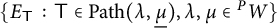
$\{ E_{\mathsf {T}} \,: \, \mathsf {T} \in \mathrm {Path}(\lambda , \underline {\mu }), \lambda , \mu \in {^PW}\}$
satisfying
$$\begin{align*}\deg E_{\mathsf{T}} = \deg \mathsf{T}.\end{align*}$$
-
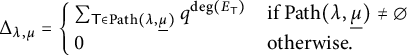
(2) The light leaves matrix can be computed follows. For any
$\lambda , \mu \in {^PW}$
we have
$$\begin{align*}\Delta_{\lambda , \mu } = \left\{\!\!\begin{array}{ll} \sum_{\mathsf{T}\in \mathrm{Path}(\lambda , \underline{\mu})} q^{\deg (E_{\mathsf{T}})} & \text{if } \mathrm{Path}(\lambda , \underline{\mu})\neq \emptyset\\ 0 & \text{otherwise.} \end{array}\right.\end{align*}$$


Thus the anti-spherical module for the oriented Temperley–Lieb algebra gives us a model to study the light leaves matrix and its factorization for all Hermitian symmetric pairs. This will be done in details in each type
 $(W,P)$
in the next few sections but first we take a short detour to relate our oriented Temperley–Lieb algebras to the generalized Temperley–Lieb algebras associated to W.
$(W,P)$
in the next few sections but first we take a short detour to relate our oriented Temperley–Lieb algebras to the generalized Temperley–Lieb algebras associated to W.
3.4 Relationship with Fan–Graham’s Temperley–Lieb algebras
We now relate our
 $(W,P)$
-Temperley–Lieb algebra to the generalized Temperley–Lieb algebra associated to W introduced by Fan (in the simply-laced type) and Graham (in the non-simply laced type).
$(W,P)$
-Temperley–Lieb algebra to the generalized Temperley–Lieb algebra associated to W introduced by Fan (in the simply-laced type) and Graham (in the non-simply laced type).
Definition 3.13 The generalized Temperley–Lieb algebra
 $\mathrm {TL}_W(q)$
is defined as the
$\mathrm {TL}_W(q)$
is defined as the
 $\mathbb {Z}[q, q^{-1}]$
-algebra generated by
$\mathbb {Z}[q, q^{-1}]$
-algebra generated by
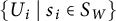 $$\begin{align*}\{U_i \mid s_i\in S_W\}\end{align*}$$
subject to the following relations: For all
 $s_i\in S_W$
we have
$s_i\in S_W$
we have
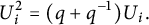 $$ \begin{align} U_i^2 = (q+q^{-1})U_i. \end{align} $$
Furthermore, we have that
 $$ \begin{align} U_iU_j = U_jU_i, \quad \quad U_iU_jU_i =U_i, \quad \quad U_iU_jU_iU_j = 2U_iU_j \end{align} $$
for
 $m_{i,j} = 2, 3 $
or
$m_{i,j} = 2, 3 $
or
 $4$
, respectively.
$4$
, respectively.
Proposition 3.14 There is a
 $\mathbb {Z}[q,q^{-1}]$
-algebra homomorphism from
$\mathbb {Z}[q,q^{-1}]$
-algebra homomorphism from
 $\mathrm {TL}_W(q)$
to
$\mathrm {TL}_W(q)$
to
 $\mathrm {TL}_{(W,P)}(q)$
defined by
$\mathrm {TL}_{(W,P)}(q)$
defined by
 $U_i\mapsto E_i$
for all
$U_i\mapsto E_i$
for all
 $s_i\in S_W$
.
$s_i\in S_W$
.
Proof We need to check that the
 $E_i$
’s satisfy the relations (3.5) and (3.6). The leftmost two relations of (3.6) are given by (3.3). The rightmost relation in (3.6) follows from Remark 3.7. It remains to show (3.5). We have
$E_i$
’s satisfy the relations (3.5) and (3.6). The leftmost two relations of (3.6) are given by (3.3). The rightmost relation in (3.6) follows from Remark 3.7. It remains to show (3.5). We have
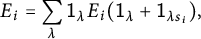 $$\begin{align*}E_i = \sum_\lambda \mathsf{1}_\lambda E_i (\mathsf{1}_\lambda + \mathsf{1}_{\lambda s_i}),\end{align*}$$
where the sum is taken over all
 $\lambda \in {^PW}$
such that
$\lambda \in {^PW}$
such that
 $\lambda s_i\in {^PW}$
. Now we have
$\lambda s_i\in {^PW}$
. Now we have
 $$ \begin{align*} E_i^2 &= \textstyle \sum_\lambda \mathsf{1}_\lambda E_i (\mathsf{1}_\lambda + \mathsf{1}_{\lambda s_i})E_i (\mathsf{1}_\lambda + \mathsf{1}_{\lambda s_i}) = (q+q^{-1}) \textstyle\sum_\lambda \mathsf{1}_\lambda E_i (\mathsf{1}_\lambda + \mathsf{1}_{\lambda s_i}) = (q+q^{-1})E_i \end{align*} $$
as required. Here the first equality follows by (3.1) and the second by (3.2), the third is trivial.
Remark 3.15 Note that this homomorphism is not injective in general. To see this, take for example W of type
 $A_3$
and P of type
$A_3$
and P of type
 $A_2$
, then
$A_2$
, then
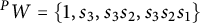 $^PW = \{ 1, s_3, s_3s_2, s_3s_2s_1\}$
. Then we claim that
$^PW = \{ 1, s_3, s_3s_2, s_3s_2s_1\}$
. Then we claim that
 $E_1E_3=0$
. To see this, note that
$E_1E_3=0$
. To see this, note that
 $E_1 \mathsf {1}_\lambda \neq 0$
implies that
$E_1 \mathsf {1}_\lambda \neq 0$
implies that
 $\lambda = s_3s_2$
or
$\lambda = s_3s_2$
or
 $s_3s_2s_1$
but
$s_3s_2s_1$
but
 $\mathsf {1}_\lambda E_3\neq 0$
implies
$\mathsf {1}_\lambda E_3\neq 0$
implies
 $\lambda = 1$
or
$\lambda = 1$
or
 $s_3$
. However,
$s_3$
. However,
 $U_1U_3\neq 0$
in
$U_1U_3\neq 0$
in
 $\mathrm {TL}_W(q)$
.
$\mathrm {TL}_W(q)$
.
4 Light leaves matrix factorization for the trivial and exceptional types
Corollary 3.12 provides a way of studying the light leaves matrix using the oriented Temperley–Lieb algebra and its anti-spherical module for all Hermitian symmetric pairs
 $(W,P)$
. In Sections 5 to 8, we will construct a diagrammatic version of the oriented Temperley–Lieb algebras in types
$(W,P)$
. In Sections 5 to 8, we will construct a diagrammatic version of the oriented Temperley–Lieb algebras in types
 $(A_n, A_k\times A_{n-k-1})$
,
$(A_n, A_k\times A_{n-k-1})$
,
 $(D_n, A_{n-1}),$
and
$(D_n, A_{n-1}),$
and
 $(C_n, A_{n-1})$
which will provide closed combinatorial formulas for the light leaves matrix and its factorization. This could also be done in types
$(C_n, A_{n-1})$
which will provide closed combinatorial formulas for the light leaves matrix and its factorization. This could also be done in types
 $(B_n, B_{n-1})$
and
$(B_n, B_{n-1})$
and
 $(D_n, D_{n-1})$
but the extra effort is unwarranted as the light leaves matrices and their factorization can be easily described without them. This will be done in this section, together with the exceptional types
$(D_n, D_{n-1})$
but the extra effort is unwarranted as the light leaves matrices and their factorization can be easily described without them. This will be done in this section, together with the exceptional types
 $(E_6, D_5)$
and
$(E_6, D_5)$
and
 $(E_7, E_6)$
, which are best tackled with a computer (although
$(E_7, E_6)$
, which are best tackled with a computer (although
 $(E_6,E_5)$
is manageable by hand as well). This provides a proof of Theorem A in these trivial and exceptional types.
$(E_6,E_5)$
is manageable by hand as well). This provides a proof of Theorem A in these trivial and exceptional types.
4.1 Exceptional types
We first consider the exceptional Hermitian symmetric pairs. One can calculate the
 $\Delta $
matrix for type
$\Delta $
matrix for type
 $(E_6,D_5)$
easily by hand. For type
$(E_6,D_5)$
easily by hand. For type
 $(E_7,E_6)$
this is a much larger calculation, but can be readily done using the Coxeter 3 package in SAGE which wraps Folko Ducloux’s original work in
$(E_7,E_6)$
this is a much larger calculation, but can be readily done using the Coxeter 3 package in SAGE which wraps Folko Ducloux’s original work in
 $C^{++}$
. The matrices
$C^{++}$
. The matrices
 $\Delta $
are recorded in Figures 5 and 6. In both cases, note that all off-diagonal entries belong to
$\Delta $
are recorded in Figures 5 and 6. In both cases, note that all off-diagonal entries belong to
 $q{\mathbb N}_0[q]$
and so
$q{\mathbb N}_0[q]$
and so
 $\Delta = N$
and
$\Delta = N$
and
 $B=\mathrm {Id}$
. This gives a proof of Theorem A in these cases by setting every basis element
$B=\mathrm {Id}$
. This gives a proof of Theorem A in these cases by setting every basis element
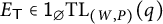 $E_{\mathsf {T}}\in \mathsf {1}_{\varnothing }\mathrm {TL}_{(W,P)}(q)$
to be standard.
$E_{\mathsf {T}}\in \mathsf {1}_{\varnothing }\mathrm {TL}_{(W,P)}(q)$
to be standard.
The light leaves matrix
 $\Delta _{\lambda , \mu }$
of type
$\Delta _{\lambda , \mu }$
of type
 $(E_6, D_5)$
. For purposes of space, we record
$(E_6, D_5)$
. For purposes of space, we record
 $q^i$
simply as i, and we record each zero polynomials as a dot. For example, the matrix is uni-triangular with diagonal entries
$q^i$
simply as i, and we record each zero polynomials as a dot. For example, the matrix is uni-triangular with diagonal entries
 $q^0=1$
. The rows and columns are ordered by a total refinement of the Bruhat order in which we prefer to add the reflection with largest possible subscript. More specifically, the order is as follows
$q^0=1$
. The rows and columns are ordered by a total refinement of the Bruhat order in which we prefer to add the reflection with largest possible subscript. More specifically, the order is as follows 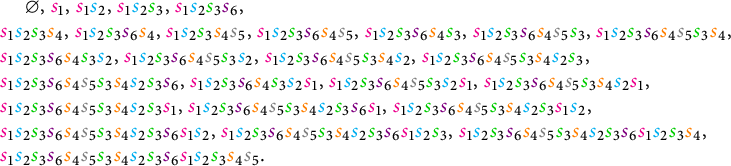
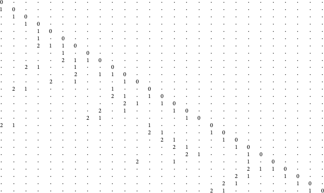
The light leaves matrix
 $\Delta $
of type
$\Delta $
of type
 $(E_7, E_6)$
. For purposes of space, we record
$(E_7, E_6)$
. For purposes of space, we record
 $q^i$
simply as i, and we record each zero polynomials as a dot. For example. the matrix is uni-triangular with diagonal entries
$q^i$
simply as i, and we record each zero polynomials as a dot. For example. the matrix is uni-triangular with diagonal entries
 $q^0=1$
. The rows and columns are ordered by a total refinement of the Bruhat order in which add the reflection with largest possible subscript.
$q^0=1$
. The rows and columns are ordered by a total refinement of the Bruhat order in which add the reflection with largest possible subscript.
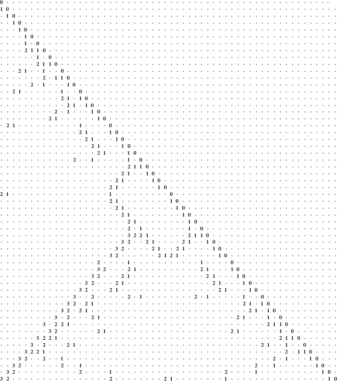
4.2 Type
$(D_n,D_{n-1})$
.

In this case, there is precisely one element in
 ${^PW}$
of each length
${^PW}$
of each length
 $0\leq \ell \leq 2(n-1)$
,
$0\leq \ell \leq 2(n-1)$
,
 $\ell \neq n-1$
and precisely two elements of length
$\ell \neq n-1$
and precisely two elements of length
 $n-1$
. Ordering the rows and columns of the matrix
$n-1$
. Ordering the rows and columns of the matrix
 $\Delta $
by decreasing length we have
$\Delta $
by decreasing length we have
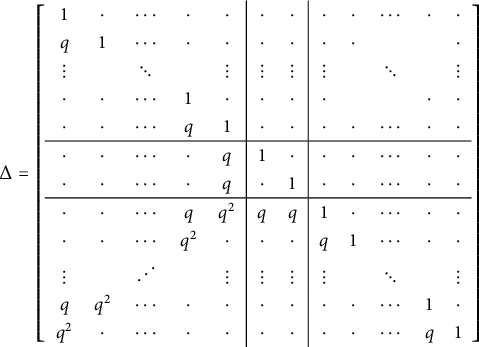 $$\begin{align*}\Delta=\left[ \begin{array}{ccccc|cc|cccccccc} 1& \cdot & \cdots & \cdot & \cdot & \cdot & \cdot & \cdot & \cdot & \cdots & \cdot & \cdot \\ q & 1 & \cdots & \cdot & \cdot & \cdot & \cdot & \cdot & \cdot & & & \cdot \\ \vdots & &\ddots & & \vdots & \vdots & \vdots & \vdots & & \ddots & & \vdots \\ \cdot & \cdot & \cdots & 1 & \cdot & \cdot & \cdot & \cdot & & & \cdot & \cdot \\ \cdot & \cdot & \cdots & q & 1 & \cdot & \cdot & \cdot & \cdot & \cdots & \cdot & \cdot \\ \hline \cdot & \cdot & \cdots & \cdot & q & 1 & \cdot & \cdot & \cdot & \cdots & \cdot & \cdot \\ \cdot & \cdot & \cdots & \cdot & q & \cdot & 1 & \cdot & \cdot & \cdots & \cdot & \cdot \\ \hline \cdot & \cdot & \cdots & q & q^2 & q&q & 1 & \cdot & \cdots & \cdot & \cdot \\ \cdot &\cdot &\cdots &q^2 &\cdot & \cdot &\cdot& q & 1 & \cdots & \cdot & \cdot \\ \vdots & &\unicode{x22F0} & &\vdots &\vdots &\vdots&\vdots & &\ddots & & \vdots \\ q &q^2 &\cdots &\cdot &\cdot &\cdot &\cdot & \cdot & \cdot & \cdots & 1 & \cdot \\ q^2 &\cdot & \cdots &\cdot &\cdot &\cdot &\cdot & \cdot & \cdot & \cdots & q & 1 \end{array}\right] \end{align*}$$
that is, the top left and bottom right
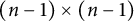 $(n-1)\times (n-1)$
-matrices have non-zero entries on the diagonal and sub-diagonal only; the bottom left
$(n-1)\times (n-1)$
-matrices have non-zero entries on the diagonal and sub-diagonal only; the bottom left
 $(n-1)\times (n-1)$
-matrix has non-zero entries on the anti-diagonal and sup-anti-diagonal only. In this case the matrix factorization is trivial, with
$(n-1)\times (n-1)$
-matrix has non-zero entries on the anti-diagonal and sup-anti-diagonal only. In this case the matrix factorization is trivial, with
 $B=\mathrm {Id}$
and
$B=\mathrm {Id}$
and
 $N=\Delta $
. This gives a proof of Theorem A in type
$N=\Delta $
. This gives a proof of Theorem A in type
 $(D_n, D_{n-1})$
by setting every basis elements in the anti-spherical module for
$(D_n, D_{n-1})$
by setting every basis elements in the anti-spherical module for
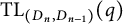 $\mathrm { TL}_{(D_n, D_{n-1})}(q)$
to be standard.
$\mathrm { TL}_{(D_n, D_{n-1})}(q)$
to be standard.
4.3 Type
$(B_n,B_{n-1})$

In this type, there is precisely one element
 $\lambda \in {^PW}$
of each length. Ordering the rows and columns of the matrix
$\lambda \in {^PW}$
of each length. Ordering the rows and columns of the matrix
 $\Delta $
by decreasing length it is easy to see that
$\Delta $
by decreasing length it is easy to see that
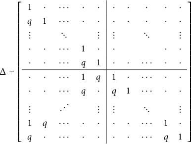 $$\begin{align*}\Delta=\left[ \begin{array}{ccccc|ccccccccc} 1& \cdot & \cdots & \cdot & \cdot & \cdot & \cdot & \cdot & \cdot & \cdot \\ q & 1 & \cdots & \cdot & \cdot & \cdot & \cdot & \cdot & \cdot & \cdot \\ \vdots & &\ddots & & \vdots & \vdots & & \ddots & & \vdots \\ \cdot & \cdot & \cdots & 1 & \cdot & \cdot & & & \cdot & \cdot \\ \cdot & \cdot & \cdots & q & 1 & \cdot & \cdot & \cdots & \cdot & \cdot \\ \hline \cdot & \cdot & \cdots & 1 & q & 1 & \cdot & \cdots & \cdot & \cdot \\ \cdot &\cdot &\cdots &q &\cdot & q & 1 & \cdots & \cdot & \cdot \\ \vdots & &\unicode{x22F0} & &\vdots &\vdots & &\ddots & & \vdots \\ 1 &q &\cdots &\cdot &\cdot & \cdot & \cdot & \cdots & 1 & \cdot \\ q &\cdot & \cdots &\cdot &\cdot & \cdot & \cdot & \cdots & q & 1 \end{array}\right] \end{align*}$$
that is, the top left and bottom right
 $n\times n$
-matrices have non-zero entries on the diagonal and sub-diagonal only; the bottom left
$n\times n$
-matrices have non-zero entries on the diagonal and sub-diagonal only; the bottom left
 $n\times n$
-matrix has non-zero entries on the anti-diagonal and sub-anti-diagonal only. We then immediately deduce that the matrix factorization is as follows
$n\times n$
-matrix has non-zero entries on the anti-diagonal and sub-anti-diagonal only. We then immediately deduce that the matrix factorization is as follows
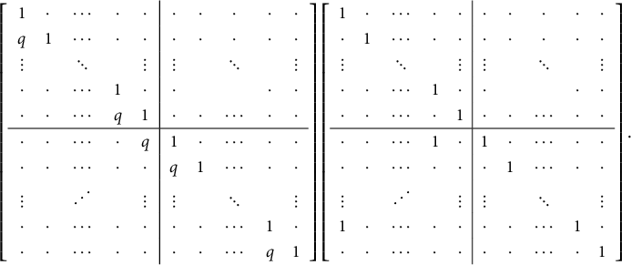 $$\begin{align*}\left[ \begin{array}{ccccc|ccccccccc} 1& \cdot & \cdots & \cdot & \cdot & \cdot & \cdot & \cdot & \cdot & \cdot \\ q & 1 & \cdots & \cdot & \cdot & \cdot & \cdot & \cdot & \cdot & \cdot \\ \vdots & &\ddots & & \vdots & \vdots & & \ddots & & \vdots \\ \cdot & \cdot & \cdots & 1 & \cdot & \cdot & & & \cdot & \cdot \\ \cdot & \cdot & \cdots & q & 1 & \cdot & \cdot & \cdots & \cdot & \cdot \\ \hline \cdot & \cdot & \cdots & \cdot & q & 1 & \cdot & \cdots & \cdot & \cdot \\ \cdot &\cdot &\cdots &\cdot &\cdot & q & 1 & \cdots & \cdot & \cdot \\ \vdots & &\unicode{x22F0} & &\vdots &\vdots & &\ddots & & \vdots \\ \cdot &\cdot &\cdots &\cdot &\cdot & \cdot & \cdot & \cdots & 1 & \cdot \\ \cdot &\cdot & \cdots &\cdot &\cdot & \cdot & \cdot & \cdots & q & 1 \end{array}\right] \left[ \begin{array}{ccccc|ccccccccc} 1& \cdot & \cdots & \cdot & \cdot & \cdot & \cdot & \cdot & \cdot & \cdot \\ \cdot & 1 & \cdots & \cdot & \cdot & \cdot & \cdot & \cdot & \cdot & \cdot \\ \vdots & &\ddots & & \vdots & \vdots & & \ddots & & \vdots \\ \cdot & \cdot & \cdots & 1 & \cdot & \cdot & & & \cdot & \cdot \\ \cdot & \cdot & \cdots & \cdot & 1 & \cdot & \cdot & \cdots & \cdot & \cdot \\ \hline \cdot & \cdot & \cdots &1 & \cdot & 1 & \cdot & \cdots & \cdot & \cdot \\ \cdot &\cdot &\cdots &\cdot &\cdot & \cdot & 1 & \cdots & \cdot & \cdot \\ \vdots & &\unicode{x22F0} & &\vdots &\vdots & &\ddots & & \vdots \\ 1 &\cdot &\cdots &\cdot &\cdot & \cdot & \cdot & \cdots & 1 & \cdot \\ \cdot &\cdot & \cdots &\cdot &\cdot & \cdot & \cdot & \cdots &\cdot & 1 \end{array}\right]. \end{align*}$$
where we note that the matrix on the left is the same as the matrix of Kazhdan–Lusztig polynomials of type
 $(A_{2n-1}, A_{2n-2})$
, this will be explained in our companion paper [Reference Bowman, De Visscher, Hazi and NortonBDHN]. This gives a proof of Theorem A in type
$(A_{2n-1}, A_{2n-2})$
, this will be explained in our companion paper [Reference Bowman, De Visscher, Hazi and NortonBDHN]. This gives a proof of Theorem A in type
 $(B_n, B_{n-1})$
by setting every basis element
$(B_n, B_{n-1})$
by setting every basis element
 $E_{\mathsf {T}}$
corresponding to non-zero entries in the matrix N (on the left) to be standard.
$E_{\mathsf {T}}$
corresponding to non-zero entries in the matrix N (on the left) to be standard.
From now, until the end of Section 8, we focus solely on the remaining cases, namely,
 $(W,P) = (A_{n}, A_{k-1}\times A_{n-k}), (C_n, A_{n-1}),$
and
$(W,P) = (A_{n}, A_{k-1}\times A_{n-k}), (C_n, A_{n-1}),$
and
 $(D_n, A_{n-1})$
.
$(D_n, A_{n-1})$
.
5 Bruhat graphs in classical type
We now introduce an elementary way of visualizing the graphs
 $\mathcal {G}_{(W,P)}$
for classical Hermitian symmetric pairs
$\mathcal {G}_{(W,P)}$
for classical Hermitian symmetric pairs
 $(W,P)=(A_n, A_{k-1}\times A_{n-k}), (C_n, A_{n-1}),$
and
$(W,P)=(A_n, A_{k-1}\times A_{n-k}), (C_n, A_{n-1}),$
and
 $(D_n, A_{n-1})$
. We will use these in the next section to define a diagrammatic visualization of the oriented Temperley–Lieb algebra in these types.
$(D_n, A_{n-1})$
. We will use these in the next section to define a diagrammatic visualization of the oriented Temperley–Lieb algebra in these types.
We start by recalling the description of the Coxeter groups of type
 $A_n, C_n,$
and
$A_n, C_n,$
and
 $D_n$
as groups of (signed) permutations. The Coxeter group of type
$D_n$
as groups of (signed) permutations. The Coxeter group of type
 $A_n$
is the symmetric group consisting of all permutations of
$A_n$
is the symmetric group consisting of all permutations of
 $\{1, 2, \ldots , n+1\}$
. The simple reflections
$\{1, 2, \ldots , n+1\}$
. The simple reflections
 $s_i$
, for
$s_i$
, for
 $1\leq i\leq n$
are given by
$1\leq i\leq n$
are given by
 $$ \begin{align*} s_i = (i, i+1). \end{align*} $$
The Coxeter group of type
 $C_n$
is the signed permutation group, namely the group of all permutations w of
$C_n$
is the signed permutation group, namely the group of all permutations w of
 $\{\pm 2, \pm 3, \ldots , \pm (n+1)\}$
such that
$\{\pm 2, \pm 3, \ldots , \pm (n+1)\}$
such that
 $w(-i)=-w(i)$
for all
$w(-i)=-w(i)$
for all
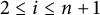 $2\leq i\leq n+1$
. The simple reflections
$2\leq i\leq n+1$
. The simple reflections
 $s_i$
for
$s_i$
for
 $i=1', 2, \ldots , n$
are given by
$i=1', 2, \ldots , n$
are given by
 $$ \begin{align*} s_{1'} = (2, -2) \quad \text{ and} \quad s_i = (i,i+1)(-i, -(i+1)) \,\,\text{for } 2 \leq i \leq n. \end{align*} $$
The Coxeter group of type
 $D_n$
is the even signed permutation group, that is the subgroup of the group of all signed permutations on
$D_n$
is the even signed permutation group, that is the subgroup of the group of all signed permutations on
 $\{\pm 1 , \pm 2, \ldots , \pm n\}$
consisting of all elements flipping an even number of signs. The simple reflections
$\{\pm 1 , \pm 2, \ldots , \pm n\}$
consisting of all elements flipping an even number of signs. The simple reflections
 $s_i$
for
$s_i$
for
 $i=1", 1 , 2, \ldots , n-1$
are given by
$i=1", 1 , 2, \ldots , n-1$
are given by
 $$\begin{align*}s_{1"} = (1, -2)(-1,2) \quad \text{and} \quad s_i = (i,i+1)(-i, -(i+1)) \,\, \text{for } 1\leq i\leq n-1.\end{align*}$$
Remark 5.1 The choice of labelling in type
 $C_n$
might seem slightly unnatural at this point but (apart from giving a uniform definition of the generators
$C_n$
might seem slightly unnatural at this point but (apart from giving a uniform definition of the generators
 $s_i$
for
$s_i$
for
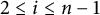 $2\leq i \leq n-1$
in all types) it is required for compatibility with the diagrammatic Temperley–Lieb algebra of type C given in Section 6.
$2\leq i \leq n-1$
in all types) it is required for compatibility with the diagrammatic Temperley–Lieb algebra of type C given in Section 6.
Given this description of the Coxeter groups as (signed) permutation groups, we have the following natural visualization of the cosets
 ${^PW}$
. We will represent elements of
${^PW}$
. We will represent elements of
 ${^PW}$
as horizontal lines with
${^PW}$
as horizontal lines with
 $n(+1)$
points in positions
$n(+1)$
points in positions
 $1, 2 , \ldots , n (,n+1)$
labeled with the symbols
$1, 2 , \ldots , n (,n+1)$
labeled with the symbols
 $\{\wedge , \vee , \circ \}$
. The generators of W will act on these as follows: For
$\{\wedge , \vee , \circ \}$
. The generators of W will act on these as follows: For
 $i\geq 1$
,
$i\geq 1$
,
 $s_i$
swaps the labels in positions i and
$s_i$
swaps the labels in positions i and
 $i+1$
, the generator
$i+1$
, the generator
 $s_{1'}$
flips (through the horizontal axis) the label in second position, and
$s_{1'}$
flips (through the horizontal axis) the label in second position, and
 $s_{1"}$
swaps and flips (through the horizontal line) the labels in first and second positions. Now, we start by representing the identity coset, which we denote by
$s_{1"}$
swaps and flips (through the horizontal line) the labels in first and second positions. Now, we start by representing the identity coset, which we denote by
 $\varnothing $
(for the empty word in the generators), as follows:
$\varnothing $
(for the empty word in the generators), as follows:
-
• If
$(W,P)=(A_n, A_{k-1}\times A_{n-k})$
, draw
$\varnothing $
as the horizontal line containing
$n+1$
points with the first k points labeled by
$\wedge $
and the last
$n-k+1$
points labeled by
$\vee $
. -
• If
$(W,P)=(C_n, A_{n-1})$
draw
$\varnothing $
as the horizontal line with
$n+1$
points with the first point labeled by
$\circ $
and the last n points labeled by
$\vee $
. -
• If
$(W,P)=(D_n , A_{n-1})$
draw
$\varnothing $
as the horizontal line with n points all labeled by
$\vee $
.


The elements of
 ${^PW}$
are then obtained as the elements of the orbit of
${^PW}$
are then obtained as the elements of the orbit of
 $\varnothing $
under the action of W.
$\varnothing $
under the action of W.
We depict the identity coset
 $\varnothing $
along the bottom of the diagram, the coset
$\varnothing $
along the bottom of the diagram, the coset
 $\lambda $
along the top of the diagram, and its corresponding reduced expression
$\lambda $
along the top of the diagram, and its corresponding reduced expression ![]() .
.
Moreover, we can construct the graph
 $\mathcal {G}_{(W,P)}$
starting from
$\mathcal {G}_{(W,P)}$
starting from
 $\varnothing $
as follows.
$\varnothing $
as follows.
-
• Start by drawing
$\varnothing $
at the bottom. -
• If applying a simple reflection does result in a new coset, then record this in the next level up in the diagram. We record the colour of the reflection as an edge relating the two points in the graph.

We repeat the above until the process terminates. This is best illustrated via the examples in Figures 8 and 9.
The Bruhat order on
 ${{^P}W}$
can also easily be visualized in this setting, namely
${{^P}W}$
can also easily be visualized in this setting, namely
 $\lambda < \mu $
if either
$\lambda < \mu $
if either
 $\lambda $
contains strictly fewer
$\lambda $
contains strictly fewer
 $\wedge $
arrows than
$\wedge $
arrows than
 $\mu $
or if
$\mu $
or if
 $\lambda $
has the same number of
$\lambda $
has the same number of
 $\wedge $
arrows as
$\wedge $
arrows as
 $\mu $
and
$\mu $
and
 $\mu $
is obtained from
$\mu $
is obtained from
 $\lambda $
by moving
$\lambda $
by moving
 $\wedge $
arrows to the right.
$\wedge $
arrows to the right.
Remark 5.2 It is worth taking a moment to consider which diagrams can appear elements of
 ${^PW}$
. It is clear that there are
${^PW}$
. It is clear that there are
 $ {n+1}\choose {k}$
cosets for
$ {n+1}\choose {k}$
cosets for
 $(A_n,A_{k-1}\times A_{n-k})$
and that these are given by all possible diagrams with
$(A_n,A_{k-1}\times A_{n-k})$
and that these are given by all possible diagrams with
 $k \wedge $
-arrows and
$k \wedge $
-arrows and
 $n-k+1 \vee $
-arrows. There are
$n-k+1 \vee $
-arrows. There are
 $ 2^n$
cosets for
$ 2^n$
cosets for
 $(C_n,A_{n-1})$
and these are given by freely choosing the
$(C_n,A_{n-1})$
and these are given by freely choosing the
 $\wedge $
versus
$\wedge $
versus
 $\vee $
decorations on the vertices
$\vee $
decorations on the vertices
 $\{ 2,\dots ,n+1\}$
(the decoration on vertex
$\{ 2,\dots ,n+1\}$
(the decoration on vertex
 $1$
is always a
$1$
is always a
 $\circ $
). There are
$\circ $
). There are
 $ 2^{n-1}$
cosets for
$ 2^{n-1}$
cosets for
 $(D_n,A_{n-1})$
and these are given by freely choosing the
$(D_n,A_{n-1})$
and these are given by freely choosing the
 $\wedge $
versus
$\wedge $
versus
 $\vee $
decorations on the vertices
$\vee $
decorations on the vertices
 $\{ 1,2,\dots ,n\}$
subject to the condition that the total number of
$\{ 1,2,\dots ,n\}$
subject to the condition that the total number of
 $\wedge $
-arrows is even.
$\wedge $
-arrows is even.
The graph
 $\mathcal {G}_{(W,P)}$
for
$\mathcal {G}_{(W,P)}$
for
 $(W,P)=(A_4,A_1 \times A_2 )$
.
$(W,P)=(A_4,A_1 \times A_2 )$
.

The graphs
 $\mathcal {G}_{(W,P)}$
for
$\mathcal {G}_{(W,P)}$
for
 $(W,P)=(D_4,A_3)$
and
$(W,P)=(D_4,A_3)$
and
 $(C_3,A_2)$
.
$(C_3,A_2)$
.
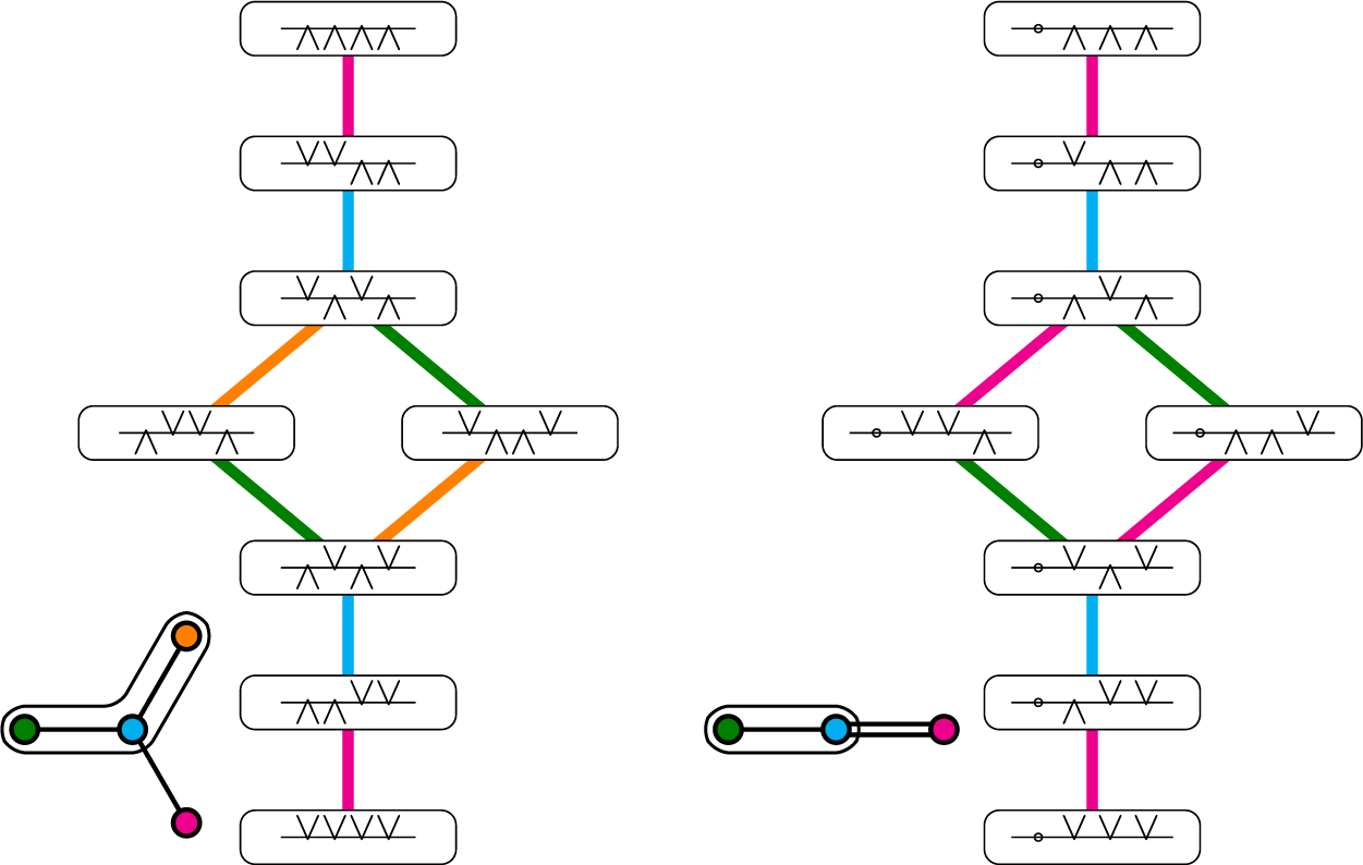
For the remainder of the paper, we will freely identify cosets with their diagrams without further mention.
Remark 5.3 In type
 $(D_n, A_{n-1})$
, the description we gave of the cosets (and graph
$(D_n, A_{n-1})$
, the description we gave of the cosets (and graph
 $\mathcal {G}_{(W,P)}$
) uses the parabolic subgroup of type
$\mathcal {G}_{(W,P)}$
) uses the parabolic subgroup of type
 $A_{n-1}$
as the subgroup generated by
$A_{n-1}$
as the subgroup generated by
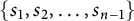 $\{s_1, s_2, \ldots , s_{n-1}\}$
. We could have used instead the parabolic subgroup of type
$\{s_1, s_2, \ldots , s_{n-1}\}$
. We could have used instead the parabolic subgroup of type
 $A_{n-1}$
generated by
$A_{n-1}$
generated by
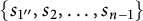 $\{s_{1"}, s_2, \ldots , s_{n-1}\}$
. This gives an alternative construction of
$\{s_{1"}, s_2, \ldots , s_{n-1}\}$
. This gives an alternative construction of
 $\mathcal {G}_{(W,P)}$
in type
$\mathcal {G}_{(W,P)}$
in type
 $(D_n, A_{n-1})$
, starting by defining the coset
$(D_n, A_{n-1})$
, starting by defining the coset
 $\varnothing $
as the horizontal line with n points where the first one is labeled by
$\varnothing $
as the horizontal line with n points where the first one is labeled by
 $\wedge $
and all others are labeled by
$\wedge $
and all others are labeled by
 $\vee $
. So the cosets now must have an odd number of
$\vee $
. So the cosets now must have an odd number of
 $\wedge $
-arrows.
$\wedge $
-arrows.
6 Diagrammatic oriented Temperley–Lieb algebras in classical type
We now introduce a visualization of oriented Temperley–Lieb algebras for
 $(W,P)$
of classical type, namely,
$(W,P)$
of classical type, namely,
 $(A_n, A_k\times A_{n-k-1})$
,
$(A_n, A_k\times A_{n-k-1})$
,
 $(D_n, A_{n-1}),$
and
$(D_n, A_{n-1}),$
and
 $(C_n, A_{n-1})$
.
$(C_n, A_{n-1})$
.
6.1 Green’s diagrammatic Temperley–Lieb algebras
We first recall Green’s diagrammatic realisation of the generalized Temperley–Lieb algebras of type W (see [Reference GreenGre98]).
Definition 6.1
-
(1) An n-tangle is a rectangular frame with n vertices on the northern and southern boundaries which are paired-off by n non-crossing strands and a finite number of non-crossing closed loops. Strands and loops can be decorated by a finite number of beads if they are left exposed (i.e., can be deformed to touch the left boundary of the frame). We refer to a strand connecting a northern and southern vertex as a propagating strand. We refer to any strand connecting two northern vertices (or two southern vertices) to each other as an arc. Two n-tangles are equal if there exists an isotopy of the plane fixing the boundaries of the frame carrying one n-tangle to the other. We denote the set of all such n-tangles by
$\mathbb {DT}_n$
. -
(2) We call an n-tangle
$d\in \mathbb {DT}_n$
undecorated if it has no beads on its strands or loops. -
(3) For R any commutative ring, we have that
$R\mathbb {DT}_n$
has the structure of an R-algebra where the multiplication is given by the vertical concatenation of n-tangles. Specifically, for
$d, d'\in \mathbb {DT}_n$
, we define the product
$d d'$
simply by placing
$d'$
above d.


Examples of undecorated tangles.

Examples of tangles. In the first and third diagrams we decorate every left-exposed strand.
We define
 $\mathsf {e}_i$
for
$\mathsf {e}_i$
for
 $i\geq 1$
to be the undecorated n-tangle with a single pair of arcs connecting the ith and
$i\geq 1$
to be the undecorated n-tangle with a single pair of arcs connecting the ith and
 $(i+1)$
th northern (respectively southern) vertices, and with
$(i+1)$
th northern (respectively southern) vertices, and with
 $(n-2)$
vertical strands. We set
$(n-2)$
vertical strands. We set
 $\mathsf {e}_{1'}=\mathsf {e}_{1"}$
to be the n-tangle which has a single pair of arcs connecting the
$\mathsf {e}_{1'}=\mathsf {e}_{1"}$
to be the n-tangle which has a single pair of arcs connecting the
 $1$
st and
$1$
st and
 $2$
nd northern (respectively southern) vertices, both of which carry a single bead, and with
$2$
nd northern (respectively southern) vertices, both of which carry a single bead, and with
 $(n-2)$
vertical undecorated strands. We use the distinct subscripts
$(n-2)$
vertical undecorated strands. We use the distinct subscripts
 $1'$
and
$1'$
and
 $1"$
to remind the reader of the corresponding Coxeter labels in Figure 1 for what follows. Examples of these elements are depicted in Figure 12.
$1"$
to remind the reader of the corresponding Coxeter labels in Figure 1 for what follows. Examples of these elements are depicted in Figure 12.
The n-tangle
 $\mathsf {e}_{1'} =\mathsf {e}_{1"} $
,
$\mathsf {e}_{1'} =\mathsf {e}_{1"} $
,
 $\mathsf {e}_1$
,
$\mathsf {e}_1$
,
 $\mathsf {e}_2$
, and
$\mathsf {e}_2$
, and
 $\mathsf {e}_3$
for
$\mathsf {e}_3$
for
 $n = 5$
.
$n = 5$
.
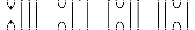
We now recall the diagrammatic visualization of the generalied Temperley–Lieb algebras
 $\mathrm {TL}_W(q)$
given in Definition 3.13. From now on, we take
$\mathrm {TL}_W(q)$
given in Definition 3.13. From now on, we take
 $R=\mathbb {Z}[q,q^{-1}]$
.
$R=\mathbb {Z}[q,q^{-1}]$
.
Theorem 6.2 (Kauffman [Reference KauffmanKau87])
The Temperley–Lieb algebra
 $\mathrm {TL}_{A_n}(q)$
of type
$\mathrm {TL}_{A_n}(q)$
of type
 $A_n$
, is isomorphic to the subquotient of the algebra
$A_n$
, is isomorphic to the subquotient of the algebra
 $R\mathbb {DT}_{n+1}$
generated by
$R\mathbb {DT}_{n+1}$
generated by
 $\mathsf {e}_1, \ldots , \mathsf {e}_n$
subject to the relation
$\mathsf {e}_1, \ldots , \mathsf {e}_n$
subject to the relation
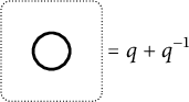
It has a basis given by the set of all undecorated
 $(n+1)$
-tangles with no loops, which we denote by
$(n+1)$
-tangles with no loops, which we denote by
 $\mathbb {DT}[A_n]$
.
$\mathbb {DT}[A_n]$
.
Theorem 6.3 (Green [Reference GreenGre98])
The generalized Temperley–Lieb algebra
 $\mathrm {TL}_{C_n}(q)$
of type
$\mathrm {TL}_{C_n}(q)$
of type
 $C_n$
is isomorphic to the subquotient of the algebra
$C_n$
is isomorphic to the subquotient of the algebra
 $R\mathbb {DT}_{n+1}$
generated by
$R\mathbb {DT}_{n+1}$
generated by
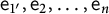 $\mathsf {e}_{1'}, \mathsf {e}_2, \ldots , \mathsf {e}_n$
subject to the relations
$\mathsf {e}_{1'}, \mathsf {e}_2, \ldots , \mathsf {e}_n$
subject to the relations
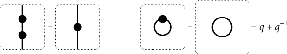
It has a basis given by the set of all
 $(n+1)$
-tangles with no loops and at most one decoration on each strand and satisfying one of the following (mutually exclusive) conditions.
$(n+1)$
-tangles with no loops and at most one decoration on each strand and satisfying one of the following (mutually exclusive) conditions.
-
(1) The leftmost northern vertex is connected to the leftmost southern vertex by an undecorated strand.
-
(2) The leftmost northern vertex is connected to the leftmost southern vertex by a decorated strand and there is at least one northern and one southern arc.
-
(3) The strands emerging from the leftmost northern and southern vertices are distinct and both decorated.
We denote the set of all such
 $(n+1)$
-tangles by
$(n+1)$
-tangles by
 $\mathbb {DT}[C_n]$
.
$\mathbb {DT}[C_n]$
.
Theorem 6.4 (Green [Reference GreenGre98])
The generalized Temperley–Lieb algebra
 $\mathrm {TL}_{D_n}(q)$
of type
$\mathrm {TL}_{D_n}(q)$
of type
 $D_n$
is isomorphic to the subquotient of the algebra
$D_n$
is isomorphic to the subquotient of the algebra
 $R\mathbb {DT}_{n}$
generated by
$R\mathbb {DT}_{n}$
generated by
 $\mathsf {e}_{1"}, \mathsf {e}_1, \mathsf {e}_2, \ldots \mathsf {e}_{n-1}$
subject to relations
$\mathsf {e}_{1"}, \mathsf {e}_1, \mathsf {e}_2, \ldots \mathsf {e}_{n-1}$
subject to relations
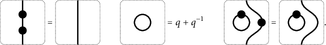
It has a basis given by the set of all n-tangles with at most one decoration on each strand or loop, and which satisfy one of the following (mutually exclusive) conditions.
-
(1) It contains one decorated loop and no other loops or decorations, and there is at least one northern and one southern arc.
-
(2) It contains no loops and the number of decorations is even.
We denote the set of all such n-tangles by
 $\mathbb {DT}[D_n]$
.
$\mathbb {DT}[D_n]$
.
6.2 Diagrammatic oriented Temperley–Lieb algebras
Recall from Section 5 that we can represent each coset representative
 $\lambda \in {^PW}$
by its coset diagram, which we also denote by
$\lambda \in {^PW}$
by its coset diagram, which we also denote by
 $\lambda $
. For
$\lambda $
. For
 $W\in \{A_n, C_n, D_n\}$
, we let
$W\in \{A_n, C_n, D_n\}$
, we let
 $\mathbb {DT}[W]$
be the set of tangles defined in Theorems 6.2 to 6.4. Now starting with any tangle in
$\mathbb {DT}[W]$
be the set of tangles defined in Theorems 6.2 to 6.4. Now starting with any tangle in
 $\mathbb {DT}[W],$
we will form so-called oriented tangles by considering elements of the form
$\mathbb {DT}[W],$
we will form so-called oriented tangles by considering elements of the form
 $\lambda d \mu $
for
$\lambda d \mu $
for
 $\lambda , \mu \in {^PW}$
by placing
$\lambda , \mu \in {^PW}$
by placing
 $\lambda $
, respectively,
$\lambda $
, respectively,
 $\mu $
on the southern, respectively, northern, boundary of d. Each strand of d in
$\mu $
on the southern, respectively, northern, boundary of d. Each strand of d in
 $\lambda d \mu $
now connects two symbols from the set
$\lambda d \mu $
now connects two symbols from the set
 $\{ \wedge , \vee , \circ \}$
from the boundaries. A strand connecting two symbols from the set
$\{ \wedge , \vee , \circ \}$
from the boundaries. A strand connecting two symbols from the set
 $\{\wedge , \vee \}$
is said to be oriented if one arrow points into the strand and the other arrow point out of the strand. We say that a strand connecting two symbols from the set
$\{\wedge , \vee \}$
is said to be oriented if one arrow points into the strand and the other arrow point out of the strand. We say that a strand connecting two symbols from the set
 $\{\wedge , \vee \}$
is flip-oriented if either both arrows point into the strand or both arrows point out of the strand. A strand connecting
$\{\wedge , \vee \}$
is flip-oriented if either both arrows point into the strand or both arrows point out of the strand. A strand connecting
 $\circ $
with one symbol from the set
$\circ $
with one symbol from the set
 $\{\wedge , \vee \}$
is said to be both oriented and flip-oriented.
$\{\wedge , \vee \}$
is said to be both oriented and flip-oriented.
Definition 6.5 For
 $d\in \mathbb {DT}[W]$
and
$d\in \mathbb {DT}[W]$
and
 $\lambda , \mu \in {^PW,}$
we say that
$\lambda , \mu \in {^PW,}$
we say that
 $\lambda d \mu $
is an oriented tangle of type
$\lambda d \mu $
is an oriented tangle of type
 $(W,P)$
if the following conditions holds.
$(W,P)$
if the following conditions holds.
-
• Every undecorated strand is oriented.
Moreover, if
 $(W,P) = (D_n, A_{n-1})$
then
$(W,P) = (D_n, A_{n-1})$
then
-
• every decorated strand is flip-oriented, and
-
• there are no loops.
If
 $(W,P)=(C_n, A_{n-1})$
then
$(W,P)=(C_n, A_{n-1})$
then
-
• there are no decorations on the strand connecting
$\circ $
to
$\circ $
.


We denote by
 $\mathbb {ODT}[W,P]$
the set of all oriented tangles of type
$\mathbb {ODT}[W,P]$
the set of all oriented tangles of type
 $(W,P)$
and refer to these as oriented Temperley–Lieb diagrams of type
$(W,P)$
and refer to these as oriented Temperley–Lieb diagrams of type
 $(W,P)$
.
$(W,P)$
.
Oriented tangles of type
 $(A_{8},A_4\times A_3)$
obtained from the diagrams of Figure 10.
$(A_{8},A_4\times A_3)$
obtained from the diagrams of Figure 10.
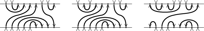
Oriented tangles of type
 $(C_{9},A_8)$
,
$(C_{9},A_8)$
,
 $(D_{10},A_9)$
, and
$(D_{10},A_9)$
, and
 $(C_8,A_7)$
, respectively, obtained by orienting the diagrams from Figure 11.
$(C_8,A_7)$
, respectively, obtained by orienting the diagrams from Figure 11.

Examples of oriented tangles are given in Figures 13 and 14.
Remark 6.6 Note that, by definition, we have that
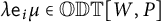 $\lambda \mathsf {e}_i \mu \in \mathbb {ODT}[W,P]$
if and only if
$\lambda \mathsf {e}_i \mu \in \mathbb {ODT}[W,P]$
if and only if
 $\lambda \xrightarrow {i} \mu $
is an edge in the graph
$\lambda \xrightarrow {i} \mu $
is an edge in the graph
 $\widehat {\mathcal {G}}_{(W,P)}$
.
$\widehat {\mathcal {G}}_{(W,P)}$
.
The following proposition follows directly from Remark 5.2.
Proposition 6.7 Let
 $d\in \mathbb {DT}[W]$
. Then there exists
$d\in \mathbb {DT}[W]$
. Then there exists
 $\lambda , \mu \in {^PW}$
such that
$\lambda , \mu \in {^PW}$
such that
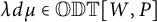 $\lambda d \mu \in \mathbb {ODT}[W,P]$
if and only if
$\lambda d \mu \in \mathbb {ODT}[W,P]$
if and only if
-
•
$(W,P) = (A_n, A_k\times A_{n-k-1})$
and d has at most
$\min \{k+1, n-k\}$
northern/southern arcs. -
•
$(W,P) = (C_n, A_{n-1})$
and d contains no decoration on a strand connecting
$\circ $
to
$\circ $
(i.e., d satisfies condition (1) or (3) from Theorem 6.3). -
•
$(W,P) = (D_n, A_{n-1})$
and d contains no loops (i.e., d satisfies condition (2) from Theorem 6.4).


We denote the set of all tangles described above by
 $\mathbb {DT}[W,P]$
.
$\mathbb {DT}[W,P]$
.
Definition 6.8 The diagrammatic oriented Temperley–Lieb algebra of type
 $(W,P)$
, denoted by
$(W,P)$
, denoted by
 $\mathrm {TL}^{{\wedge }{\vee }}_{(W,P)}(q)$
, is the
$\mathrm {TL}^{{\wedge }{\vee }}_{(W,P)}(q)$
, is the
 $\mathbb {Z}[q,q^{-1}]$
-algebra with basis
$\mathbb {Z}[q,q^{-1}]$
-algebra with basis
 $\mathbb {ODT}[W,P]$
and multiplication defined as follows. For
$\mathbb {ODT}[W,P]$
and multiplication defined as follows. For
 $\lambda d \mu , \lambda ' d' \mu '\in \mathbb {ODT}[W,P]$
we have
$\lambda d \mu , \lambda ' d' \mu '\in \mathbb {ODT}[W,P]$
we have
 $$ \begin{align} (\lambda d \mu)(\lambda' d' \mu')=0 \quad \text{if } \mu \neq \lambda' \end{align} $$
and vertical concatenation, denoted by
 $\lambda d \mu d' \mu '$
, if
$\lambda d \mu d' \mu '$
, if
 $\mu = \lambda '$
, subject to the following relations.
$\mu = \lambda '$
, subject to the following relations.
-
(1) Closed loop relation. Remove any closed loop and replace it by q if its rightmost vertex is labeled by
$\vee $
, and by
$q^{-1}$
if its rightmost vertex is labeled by
$\wedge $
. Once all closed loops have been removed, delete all remaining symbols coming from
$\mu = \lambda '$
and apply the following relations. -
(2) Double bead relation. We have that
in types
$C_n$
and
$D_n,$
respectively. -
(3) Non-simply laced bead relation. In type
$C_n$
, we have that


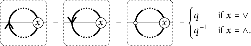

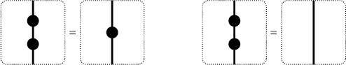


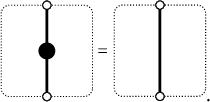
Remark 6.9 Note that the multiplication is associative. Indeed, consider the product of three oriented tangles forming a closed loop as pictured below. Then we have that the red zigzag-strand is not left-exposed and so must be oriented. This implies that the symbols at x and y are either both
 $\wedge $
or both
$\wedge $
or both
 $\vee $
and hence we will get the same result whichever way we apply the two multiplications.
$\vee $
and hence we will get the same result whichever way we apply the two multiplications.
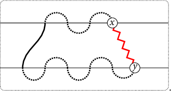
Therefore
 $\mathrm {TL}^{{\wedge }{\vee }}_{(W,P)}(q)$
is a unital associative algebra with identity
$\mathrm {TL}^{{\wedge }{\vee }}_{(W,P)}(q)$
is a unital associative algebra with identity
 $\sum _{\lambda \in {^PW}} \lambda \mathsf {1}\lambda $
where
$\sum _{\lambda \in {^PW}} \lambda \mathsf {1}\lambda $
where
 $\mathsf {1}$
is the tangle in
$\mathsf {1}$
is the tangle in
 $\mathbb {DT}(W)$
containing only undecorated propagating strands (that is, the identity element in
$\mathbb {DT}(W)$
containing only undecorated propagating strands (that is, the identity element in
 $\mathrm {TL}_{W}(q)$
).
$\mathrm {TL}_{W}(q)$
).
Definition 6.10 We define the parity specialization map
 $$ \begin{align*}{^{A_{n-1}}C_n}\to{ ^{A_{n}}D_{n+1}} \qquad :\lambda \mapsto \overline{\lambda}\end{align*} $$
by replacing the
 $\circ $
in
$\circ $
in
 $\lambda $
by either an
$\lambda $
by either an
 $\wedge $
or
$\wedge $
or
 $\vee $
arrow in such a way that the resulting total number of
$\vee $
arrow in such a way that the resulting total number of
 $\wedge $
arrows is even.
$\wedge $
arrows is even.
We note that the parity specialization map is a bijection between our diagrammatic coset representatives, by definition.
In Section 8, we will see that whilst the matrices of light leaves polynomials of types
 $(D_{n+1},A_n)$
and
$(D_{n+1},A_n)$
and
 $(C_n,A_{n-1})$
are genuinely distinct, the underlying Kazhdan–Lusztig polynomials are the same (see also [Reference BoeBoe88, Reference Ehrig and StroppelES16a]). The key to understanding this phenomenon will be the following.
$(C_n,A_{n-1})$
are genuinely distinct, the underlying Kazhdan–Lusztig polynomials are the same (see also [Reference BoeBoe88, Reference Ehrig and StroppelES16a]). The key to understanding this phenomenon will be the following.
Proposition 6.11 There is a surjective algebra homomorphism
 $$\begin{align*}\varphi:\mathrm{TL}_{(C_n,A_{n-1})}^{\wedge\vee}(q)\to \mathrm{TL}_{(D_{n+1},A_{n})}^{\wedge\vee}(q)\end{align*}$$
by setting
 $\varphi (\lambda d \mu )$
to be the oriented tangle obtained from
$\varphi (\lambda d \mu )$
to be the oriented tangle obtained from
 $\overline \lambda d \overline \mu $
by removing the beads from all decorated oriented strands.
$\overline \lambda d \overline \mu $
by removing the beads from all decorated oriented strands.
Proof Clearly the map is surjective. We now verify that
 $\varphi $
preserves the relations. The closed loops relation is trivially preserved as it only involves the rightmost decoration on the loop, which is unchanged by the parity specialization map. (6.1) is also trivially preserved. We now verify the bead relations of Definition 6.8. We slightly abuse notation by setting d to be the tangle consisting of a single decorated propagating strand and by setting u to be the tangle consisting of a single undecorated propagating strand. We check that
$\varphi $
preserves the relations. The closed loops relation is trivially preserved as it only involves the rightmost decoration on the loop, which is unchanged by the parity specialization map. (6.1) is also trivially preserved. We now verify the bead relations of Definition 6.8. We slightly abuse notation by setting d to be the tangle consisting of a single decorated propagating strand and by setting u to be the tangle consisting of a single undecorated propagating strand. We check that
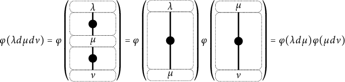
by breaking this up into three cases depending on
 $\lambda ,\mu ,\nu \in \{\circ ,\wedge ,\vee \}$
. Note that
$\lambda ,\mu ,\nu \in \{\circ ,\wedge ,\vee \}$
. Note that
 $\overline {\lambda },\overline {\mu },\overline {\nu }$
depend on the entirety of the coset diagram, not just the label of the strand that we are considering (as they are calculated by the overall parity). The three cases are as follows:
$\overline {\lambda },\overline {\mu },\overline {\nu }$
depend on the entirety of the coset diagram, not just the label of the strand that we are considering (as they are calculated by the overall parity). The three cases are as follows:
-
(i) If
$\overline \lambda =\overline \mu =\overline \nu $
then
$\overline \lambda d \overline \mu $
,
$\overline \mu d\overline \nu $
, and
$\overline \lambda d\overline \nu $
are oriented strands and so
$$\begin{align*}\varphi(\lambda d \mu d \nu)= \varphi(\lambda d \nu) = \overline{\lambda} u \overline{\nu} = (\overline{\lambda} u \overline{\mu}) ( \overline{\mu} u \overline{\nu})= \varphi(\lambda d \mu) \varphi(\mu d \nu) .\end{align*}$$
-
(ii) If
$\overline \lambda =\overline \mu \neq \overline \nu $
then
$\overline \lambda d \overline \mu $
is oriented and
$\overline \lambda d\overline \nu $
,
$\overline \mu d\overline \nu $
are unoriented strands and so
$$\begin{align*}\varphi(\lambda d \mu d \nu)= \varphi(\lambda d \nu) = \overline{\lambda} d \overline{\nu} = (\overline{\lambda} u \overline{\mu}) ( \overline{\mu} d \overline{\nu})= \varphi(\lambda d \mu) \varphi(\mu d \nu) .\end{align*}$$
-
(iii) If
$\overline \lambda \neq \overline \mu \neq \overline \nu $
then
$\overline \lambda d\overline \nu $
is oriented and
$\overline \lambda d \overline \mu $
,
$\overline \mu d\overline \nu $
are unoriented strands and so
$$ \begin{align*} \varphi(\lambda d \mu d \nu)= \varphi(\lambda d \nu) = \overline{\lambda} u \overline{\nu} = (\overline{\lambda} d \overline{\mu}) ( \overline{\mu} d \overline{\nu})= \varphi(\lambda d \mu) \varphi(\mu d \nu). \end{align*} $$


The result follows.
We now state the main result of this section, which establishes that the abstract and diagrammatically defined algebras are, in fact, isomorphic. Recall, from Remark 6.6 that for any edge
 $\lambda \xrightarrow {i} \mu $
in the graph
$\lambda \xrightarrow {i} \mu $
in the graph
 $\widehat {\mathcal {G}}_{(W,P)}$
we have an element
$\widehat {\mathcal {G}}_{(W,P)}$
we have an element
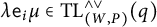 $\lambda \mathsf {e}_i \mu \in \mathrm {TL}^{\wedge \vee }_{(W,P)}(q)$
. More generally, for any path
$\lambda \mathsf {e}_i \mu \in \mathrm {TL}^{\wedge \vee }_{(W,P)}(q)$
. More generally, for any path
 $T = \lambda _1 \xrightarrow {i_1} \lambda _2 \xrightarrow {i_2} \ldots \lambda _{i_{k-1}}\xrightarrow {i_{k-1}} \lambda _k$
on the graph
$T = \lambda _1 \xrightarrow {i_1} \lambda _2 \xrightarrow {i_2} \ldots \lambda _{i_{k-1}}\xrightarrow {i_{k-1}} \lambda _k$
on the graph
 $\widehat {\mathcal {G}}_{(W,P)},$
we can form the product
$\widehat {\mathcal {G}}_{(W,P)},$
we can form the product
 $$\begin{align*}\mathsf{e}_{\mathsf{T}} := \lambda_1 \mathsf{e}_{i_1} \lambda_2 \mathsf{e}_{i_2} \ldots \lambda_{i_{k-1}}\mathsf{e}_{i_{k-1}} \lambda_k \in \mathrm{TL}^{\wedge \vee}_{(W,P)}(q).\end{align*}$$
Theorem 6.12 Let
 $(W,P)=(A_n, A_k\times A_{n-k-1}), (C_n, A_{n-1}),$
or
$(W,P)=(A_n, A_k\times A_{n-k-1}), (C_n, A_{n-1}),$
or
 $(D_n, A_{n-1})$
. There is an isomorphism of
$(D_n, A_{n-1})$
. There is an isomorphism of
 $\mathbb {Z}[q,q^{-1}]$
-algebras
$\mathbb {Z}[q,q^{-1}]$
-algebras
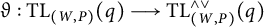 $$\begin{align*}\vartheta: \mathrm{TL}_{(W,P)}(q) \longrightarrow \mathrm{TL}^{{\wedge}{\vee}}_{(W,P)}(q)\end{align*}$$
defined by
 $\vartheta (\mathsf {1}_\lambda ) = \lambda \mathsf {1}\lambda $
, and
$\vartheta (\mathsf {1}_\lambda ) = \lambda \mathsf {1}\lambda $
, and
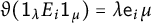 $\vartheta (\mathsf {1}_\lambda E_i \mathsf {1}_\mu ) = \lambda \mathsf {e}_i \mu $
. In particular, for any
$\vartheta (\mathsf {1}_\lambda E_i \mathsf {1}_\mu ) = \lambda \mathsf {e}_i \mu $
. In particular, for any
 $\mathsf {T}\in \mathrm {Path}_{(W,P)}$
we have
$\mathsf {T}\in \mathrm {Path}_{(W,P)}$
we have
 $\vartheta (E_{\mathsf {T}}) = \mathsf {e}_{\mathsf {T}}$
.
$\vartheta (E_{\mathsf {T}}) = \mathsf {e}_{\mathsf {T}}$
.
Remark 6.13 Note that we have
 $\vartheta (E_i) =\vartheta (\sum _\lambda (\mathsf {1}_\lambda E_i \mathsf {1}_\lambda + \lambda E_i (\mathsf {1}_{\lambda s_i}))) = \sum _\lambda (\lambda \mathsf {e}_i \lambda +\lambda \mathsf {e}_i (\lambda s_i))$
where the sum is over all
$\vartheta (E_i) =\vartheta (\sum _\lambda (\mathsf {1}_\lambda E_i \mathsf {1}_\lambda + \lambda E_i (\mathsf {1}_{\lambda s_i}))) = \sum _\lambda (\lambda \mathsf {e}_i \lambda +\lambda \mathsf {e}_i (\lambda s_i))$
where the sum is over all
 $\lambda \in {^PW}$
with
$\lambda \in {^PW}$
with
 $\lambda s_i \in {^PW}$
.
$\lambda s_i \in {^PW}$
.
We will prove this theorem in the rest of this section.
Proposition 6.14 The map
 $\vartheta $
is a
$\vartheta $
is a
 $\mathbb {Z}[q,q^{-1}]$
-algebra homomorphism.
$\mathbb {Z}[q,q^{-1}]$
-algebra homomorphism.
Proof We need to check that the relations (3.1)–(3.4) are preserved under
 $\vartheta $
. The two leftmost relations in (3.1) are clear by definition of the multiplication in
$\vartheta $
. The two leftmost relations in (3.1) are clear by definition of the multiplication in
 $\mathrm { TL}^{{\wedge }{\vee }}_{(W,P)}(q)$
. The two rightmost ones follow from the description of the graph
$\mathrm { TL}^{{\wedge }{\vee }}_{(W,P)}(q)$
. The two rightmost ones follow from the description of the graph
 $\mathcal {G}_{(W,P)}$
given in Section 5. Relation (3.2) is satisfied by the closed loop relation noting that
$\mathcal {G}_{(W,P)}$
given in Section 5. Relation (3.2) is satisfied by the closed loop relation noting that
 $\vee \vee < \wedge \wedge $
and
$\vee \vee < \wedge \wedge $
and
 $\wedge \vee < \vee \wedge $
. The leftmost relation in (3.3) holds as the corresponding tangles are isotopic for
$\wedge \vee < \vee \wedge $
. The leftmost relation in (3.3) holds as the corresponding tangles are isotopic for
 $\{i,j\}\neq \{1, 1"\}$
. Note that when
$\{i,j\}\neq \{1, 1"\}$
. Note that when
 $\{i,j\} = \{1, 1"\}$
in type
$\{i,j\} = \{1, 1"\}$
in type
 $(D_n, A_{n-1})$
, we have that
$(D_n, A_{n-1})$
, we have that
 $E_1\mathsf {1}_\lambda E_{1"} = E_{1"}\mathsf {1}_\lambda E_1= 0$
for all
$E_1\mathsf {1}_\lambda E_{1"} = E_{1"}\mathsf {1}_\lambda E_1= 0$
for all
 $\lambda \in {^PW}$
, so
$\lambda \in {^PW}$
, so
 $E_1E_{1"} = E_{1"}E_1 = 0$
and there is nothing to check. The rightmost relation in (3.3) is also satisfied using the fact that the corresponding tangles are isotopic and the double bead relation when
$E_1E_{1"} = E_{1"}E_1 = 0$
and there is nothing to check. The rightmost relation in (3.3) is also satisfied using the fact that the corresponding tangles are isotopic and the double bead relation when
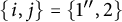 $\{i,j\} = \{1", 2\}$
in type
$\{i,j\} = \{1", 2\}$
in type
 $(D_n, A_{n-1})$
. Relation (3.4) only applies when
$(D_n, A_{n-1})$
. Relation (3.4) only applies when
 $i=2$
and
$i=2$
and
 $j=1'$
in type
$j=1'$
in type
 $(C_n, A_{n-1})$
. Now, it is easy to see that it holds in the diagrammatic algebra using isotopy, the double bead relations in type
$(C_n, A_{n-1})$
. Now, it is easy to see that it holds in the diagrammatic algebra using isotopy, the double bead relations in type
 $C_n$
and the non-simply laced bead relation.
$C_n$
and the non-simply laced bead relation.
To show that
 $\vartheta $
is an isomorphism, we will need to show that every oriented Temperley–Lieb diagram can be written as a product of generators. We start with the non-oriented diagrams.
$\vartheta $
is an isomorphism, we will need to show that every oriented Temperley–Lieb diagram can be written as a product of generators. We start with the non-oriented diagrams.
6.3 Closed and iterative constructions of Temperley–Lieb diagrams
For
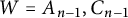 $W=A_{n-1}, C_{n-1}$
or
$W=A_{n-1}, C_{n-1}$
or
 $D_n$
, we consider a tiling of a vertical strip of the plane with square tiles labeled by the simple reflections
$D_n$
, we consider a tiling of a vertical strip of the plane with square tiles labeled by the simple reflections
 $s\in S_{W}$
as illustrated in Figure 15.
$s\in S_{W}$
as illustrated in Figure 15.
The Temperley–Lieb algebra tiling pictures for types
 $A_9$
,
$A_9$
,
 $D_{10}$
, and
$D_{10}$
, and
 $C_9,$
respectively.
$C_9,$
respectively.

Now, for
 $(W,P)=(A_{n-1}, A_{k-1}\times A_{n-k-1})$
,
$(W,P)=(A_{n-1}, A_{k-1}\times A_{n-k-1})$
,
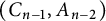 $(C_{n-1}, A_{n-2})$
or
$(C_{n-1}, A_{n-2})$
or
 $(D_n, A_{n-1})$
and
$(D_n, A_{n-1})$
and
 $d\in \mathbb {DT}[W,P]$
we have that d has n vertices on the northern edge, labeled by
$d\in \mathbb {DT}[W,P]$
we have that d has n vertices on the northern edge, labeled by
 $1, \ldots , n$
(from left to right) and n vertices on the southern edge, labeled by
$1, \ldots , n$
(from left to right) and n vertices on the southern edge, labeled by
 $1', \ldots , n'$
(from left to right). We write
$1', \ldots , n'$
(from left to right). We write
 $i'\geq j'$
whenever
$i'\geq j'$
whenever
 $i\geq j$
. Each such diagram d will correspond to a finite region on our tiling with boundary given by the path
$i\geq j$
. Each such diagram d will correspond to a finite region on our tiling with boundary given by the path
 $$\begin{align*}\pi(d) = (\pi(1), \pi(2), \ldots , \pi(n), \pi(n') , \pi((n-1)'), \ldots, \pi(2'), \pi(1'))\end{align*}$$
defined as follows: Start at the leftmost corner of a tile labeled by
 $1$
, or
$1$
, or
 $1'$
if
$1'$
if
 $W=C_{n-1}$
, then for
$W=C_{n-1}$
, then for
 $1\leq k \leq n$
we have
$1\leq k \leq n$
we have
 $$\begin{align*}\pi(k) = \left\{ \begin{array}{ll} \mathrm{NE} & \text{if } k \text{ is connected to a vertex } l>k \text{or} l'\geq k' \text{ by an undecorated strand}\\ \mathrm{SE} & \text{otherwise}. \end{array}\right.\end{align*}$$
 $$\begin{align*}\pi(k') = \left\{ \begin{array}{@{}ll} \mathrm{NW} & \text{if } k' \text{ is connected to a vertex } l>k \text{or} l'>k' \text{ by an undecorated strand}\\ \mathrm{SW} & \text{otherwise}. \end{array}\right.\end{align*}$$
Examples are given in Figures 16 and 17. We have drawn vertical lines through all tiles not included in
 $R(d)$
. We see that the vertical line starting at vertex i, respectively
$R(d)$
. We see that the vertical line starting at vertex i, respectively
 $i'$
meets the path
$i'$
meets the path
 $\pi $
at
$\pi $
at
 $\pi (i)$
, respectively
$\pi (i)$
, respectively
 $\pi (i')$
for each
$\pi (i')$
for each
 $1\leq i\leq n$
.
$1\leq i\leq n$
.
The tilings of the diagrams from Figure 13. In each case the path begins at the western-most point, which is denoted with a circle; the path then follows the orientation depicted on the diagram. An example of the associated
 $\mathsf {e}_{\underline {w}}$
for the rightmost diagram is
$\mathsf {e}_{\underline {w}}$
for the rightmost diagram is ![]() .
.
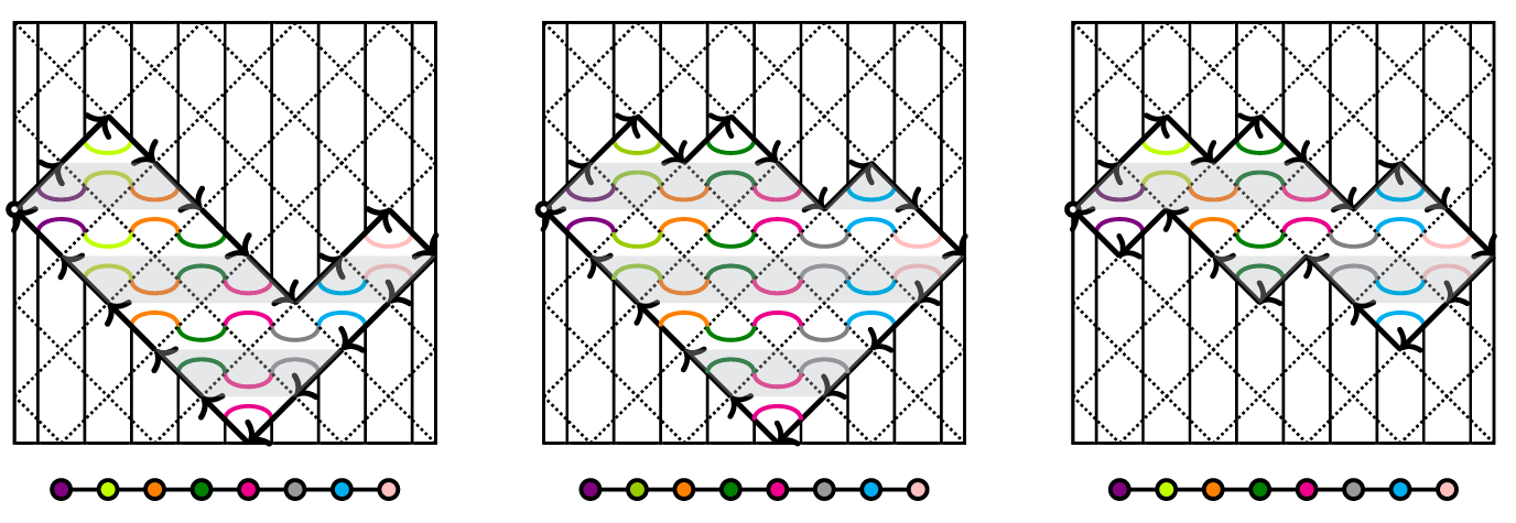
The tiling of the two leftmost diagrams from Figure 14 and an additional one in type
 $(C_9,A_8)$
. The path begins at the northerly western-most point; the path then follows the orientation depicted on the diagram until terminating at the southernly western-most point (both of which are denoted with circles). Some of the strands in type C carry two dots which can be simplified to one dot.
$(C_9,A_8)$
. The path begins at the northerly western-most point; the path then follows the orientation depicted on the diagram until terminating at the southernly western-most point (both of which are denoted with circles). Some of the strands in type C carry two dots which can be simplified to one dot.
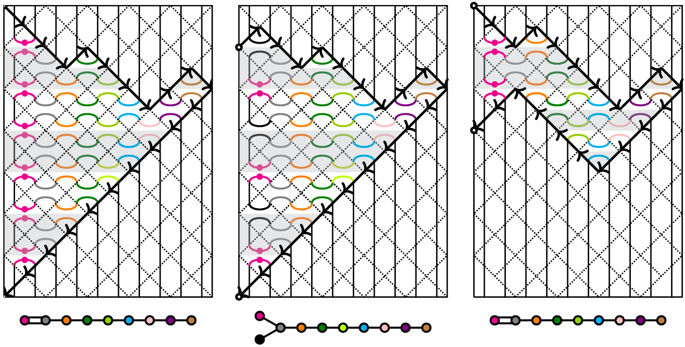
Given a subset
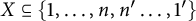 $X \subseteq \{1,\dots , n , n' \dots , 1'\}$
we set
$X \subseteq \{1,\dots , n , n' \dots , 1'\}$
we set
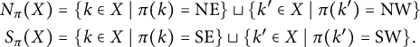 $$ \begin{align*} N_\pi (X) &= \{ k\in X \mid \pi (k)= \mathrm{NE}\} \sqcup\{ k' \in X \mid \pi (k')=\mathrm{NW}\} \\ S_\pi (X) &= \{ k\in X \mid \pi (k)= \mathrm{SE}\} \sqcup\{ k'\in X \mid \pi (k')=\mathrm{SW}\}. \end{align*} $$
First note that the path
 $\pi (d)$
takes n steps to the East and n steps to the West. So the path starts and finishes on the left boundary of the tiling. Moreover, the number of steps to the North is precisely the number of undecorated strands in d. So if d is an undecorated n-tangle, then the path starts and ends at the same point; this is because
$\pi (d)$
takes n steps to the East and n steps to the West. So the path starts and finishes on the left boundary of the tiling. Moreover, the number of steps to the North is precisely the number of undecorated strands in d. So if d is an undecorated n-tangle, then the path starts and ends at the same point; this is because
 $$\begin{align*}|N_ \pi\{1,\dots, n,n',\dots 1'\}|=n \qquad | S_ \pi\{1,\dots, n,n',\dots 1'\}|=2n-n=n. \end{align*}$$
But if d has at least one bead, then the path will end strictly below where it started, this is because in this case
 $$\begin{align*}|N_ \pi\{1,\dots, n,n',\dots 1'\} |< n \qquad |S_ \pi\{1,\dots, n,n',\dots 1'\}|>2n-n=n. \end{align*}$$
More generally, the second half of the path (going West) is always weakly to the South of the first half of the path (going East). To see this, observe that for
 $1\leq k\leq n$
, the difference in height in the path after k steps and after
$1\leq k\leq n$
, the difference in height in the path after k steps and after
 $2n-k$
steps is equal to
$2n-k$
steps is equal to
 $$\begin{align*}|S_ \pi\{k+1,\dots, n,n',\dots (k+1)'\} |- | N_ \pi\{k+1,\dots, n,n',\dots (k+1)'\} |\geq 0 \end{align*}$$
where the inequality follows by definition as every l (or
 $l'$
) in
$l'$
) in
 $N_ \pi \{k+1,\dots , n,n',\dots (k+1)'\}$
is connected to a vertex in
$N_ \pi \{k+1,\dots , n,n',\dots (k+1)'\}$
is connected to a vertex in
 $S_ \pi \{k+1,\dots , n,n',\dots (k+1)'\}$
. Thus
$S_ \pi \{k+1,\dots , n,n',\dots (k+1)'\}$
. Thus
 $\pi (d)$
defines a region
$\pi (d)$
defines a region
 $R(d)$
in the tiling which contains a finite set of tiles
$R(d)$
in the tiling which contains a finite set of tiles
 $t_1, \ldots , t_r$
(which are labeled by simple reflections in
$t_1, \ldots , t_r$
(which are labeled by simple reflections in
 $S_W$
).
$S_W$
).
We now explain how the region
 $R(d)$
defines a reduced word of a strongly fully commutative element of W. Enumerate the tiles in
$R(d)$
defines a reduced word of a strongly fully commutative element of W. Enumerate the tiles in
 $R(d)$
,
$R(d)$
,
 $t_{i_1}, \ldots , t_{i_r}$
, in such a way that for each j, the tiles in
$t_{i_1}, \ldots , t_{i_r}$
, in such a way that for each j, the tiles in
 $R(d)$
to the
$R(d)$
to the
 $\mathrm {SW}$
and
$\mathrm {SW}$
and
 $\mathrm {SE}$
of
$\mathrm {SE}$
of
 $t_{i_j}$
appear before
$t_{i_j}$
appear before
 $t_{i_j}$
. Taking the corresponding ordered product of simple reflections gives a word
$t_{i_j}$
. Taking the corresponding ordered product of simple reflections gives a word
 $\underline {w}=\underline {w}(d)$
in the elements of
$\underline {w}=\underline {w}(d)$
in the elements of
 $S_W$
. There is, of course, more than one way of enumerating the tiles in
$S_W$
. There is, of course, more than one way of enumerating the tiles in
 $R(d)$
in this fashion and these give (all the) different reduced expressions for the same element of W (as they differ only by commutation relations).
$R(d)$
in this fashion and these give (all the) different reduced expressions for the same element of W (as they differ only by commutation relations).
Conversely, any expression
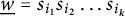 $\underline {w} = s_{i_1}s_{i_2} \ldots s_{i_k}$
with
$\underline {w} = s_{i_1}s_{i_2} \ldots s_{i_k}$
with
 $s_{i_j}\in S_W$
defines a region
$s_{i_j}\in S_W$
defines a region
 $R(\underline {w})$
in the tiling by picking any horizontal line in the tiling and stacking the boxes in order, starting from
$R(\underline {w})$
in the tiling by picking any horizontal line in the tiling and stacking the boxes in order, starting from
 $s_{i_1}$
, then
$s_{i_1}$
, then
 $s_{i_2}$
, …, and finally
$s_{i_2}$
, …, and finally
 $s_{i_k}$
. (This is an alternative description of the ‘heaps’ introduced by Stembridge [Reference StembridgeSte96]).
$s_{i_k}$
. (This is an alternative description of the ‘heaps’ introduced by Stembridge [Reference StembridgeSte96]).
Proposition 6.15
-
(1) Let
$\underline {w}$
is a reduced expression for a strongly fully commutative element of W such that
$\underline {w} = \omega (\mathsf {T})$
for some
$T\in \mathrm {Path}_{(W,P)}$
. Then
$R(\underline {w})$
does not have a boundary containing an inadmissible section of the form depicted in Figure 18.Figure 18:We emphasise the inadmissible section of the border-region by drawing it thickly. In type
$A_{n-1},$
we require that there is no such region for any
$i,j \in \{1,2,\dots ,n-1\}$
. In type
$D_{n,}$
we require that there is no such region for any
$i \in \{2,\dots ,n-1\}$
or
$j \in \{2,\dots ,n-1\}$
. In type
$C_{n-1,}$
we require that there is no such region for any
$i \in \{1',2,\dots ,n-1\}$
or
$j \in \{2,\dots ,n-1\}$
. We note that the latter two regions (involving a
$1$
and a
$1"$
tile) occur only in type
$D_{n-1}$
. -
(2) For any
$d\in \mathbb {DT}[W,P]$
, the region
$R(d)$
does not have a boundary containing an inadmissible section of the form depicted in Figure 18. In particular,
$\underline {w}(d)$
is a reduced expression for a strongly fully commutative element of W. -
(3) For any
$d\in \mathbb {DT}[W,P]$
, if
$\underline {w}(d) = \underline {w} = s_{i_1} s_{i_2} \ldots s_{i_k}$
then we have
$$\begin{align*}d = \mathsf{e}_{\underline{w}} := \mathsf{e}_{i_1} \mathsf{e}_{i_2} \ldots \mathsf{e}_{i_k}.\end{align*}$$
Moreover, if
$\underline {w'}$
is another reduced expression for the same strongly fully commutative element of W then
$\mathsf {e}_{\underline {w'}} = \mathsf {e}_{\underline {w}}$
.


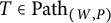


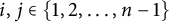

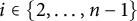
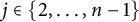

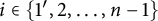


Proof
-
(1) The conditions on
$i,j$
follow from Definition 3.1 and the definition of a reduced expression (see Section 2). For the conditions involving
$1$
and
$1"$
, we note that any path on
$\widehat {\mathcal {G}}_{(D_n, A_{n-1})}$
containing an
$s_1$
-step and an
$s_{1"}$
-step must contain an
$s_2$
-step in between. -
(2) Note that the path
$\pi (d)$
takes all steps to the East first, followed by all steps to the West, this implies that boundary of
$R(d)$
does not contain any inadmissible sections and hence
$\underline {w}(d)$
is a reduced expression for a fully commutative element of W. -
(3) Now recall that for each simple reflection
$s_i\in S_W$
, we have a generator
$\mathsf {e}_i\in \mathrm {TL}_{W}(q)$
, and so any reduced expression
$\underline {w} = s_{i_1}s_{i_2} \ldots s_{i_k}$
for a strongly fully commutative element of W define a product of the generators,
$\mathsf {e}_{\underline {w}} = \mathsf {e}_{i_1} \mathsf {e}_{i_2} \ldots \mathsf {e}_{i_k}\in \mathrm {TL}_W(q)$
. These are pictured in Figures 16 and 17 for
$\underline {w} = \underline {w}(d)$
. Again, it is clear that for a different choice of reduced word
$\underline {w}'$
we have
$\mathsf {e}_{\underline {w}'} = \mathsf { e}_{\underline {w}}$
(as these differ only by commutation relations). We claim that
$\mathsf {e}_{\underline {w}} = d$
. To see this, we first partition the region
$R(d)$
by splitting it along the horizontal lines through the vertices of the tiles. This gives a partition of
$R(d)$
into horizontal strips. If a strip intersects the left boundary in more than one point, merge it with the strip above or below so that the new wider strip now contains precisely two vertices of tiles on the left boundary. These strips are shown in Figures 16 and 17 (by alternating between grey and white shading). It is clear that the strands in
$\mathsf {e}_{\underline {w}}$
are in one-to-one correspondence with the strips of
$R(d)$
. Each strip contains precisely two edges of the path
$\pi (d)$
and joins the corresponding vertices in d; one thus recovers the (decorated) n-tangle d.


Proposition 6.16 Let
 $\underline {w}$
be a reduced expression for a strongly fully commutative element of W. Suppose that we have
$\underline {w}$
be a reduced expression for a strongly fully commutative element of W. Suppose that we have
 $\lambda , \mu \in {^PW}$
with
$\lambda , \mu \in {^PW}$
with
 $\lambda \mathsf {e}_{\underline {w}}\mu \in \mathbb {ODT}[W,P]$
. Then there is a unique path
$\lambda \mathsf {e}_{\underline {w}}\mu \in \mathbb {ODT}[W,P]$
. Then there is a unique path
 $\mathsf {T}$
on
$\mathsf {T}$
on
 $\widehat {\mathcal {G}}_{(W,P)}$
starting at
$\widehat {\mathcal {G}}_{(W,P)}$
starting at
 $\lambda $
and ending at
$\lambda $
and ending at
 $\mu $
with
$\mu $
with
 $w(\mathsf {T}) = \underline {w}$
. Moreover, we have
$w(\mathsf {T}) = \underline {w}$
. Moreover, we have
 $\lambda \mathsf {e}_{\underline {w}} \mu = \mathsf {e}_{\mathsf {T}}$
.
$\lambda \mathsf {e}_{\underline {w}} \mu = \mathsf {e}_{\mathsf {T}}$
.
Proof Having fixed the orientation at the top and bottom of the product of generators
 $\mathsf {e}_{\underline {w}}$
, there are only two situations in which we have a choice of orientation for strand segments in this product. The first one is when the diagram contains a closed loop. These are formed by a tile configuration of the form depicted on the left of Figure 19. The second one is when
$\mathsf {e}_{\underline {w}}$
, there are only two situations in which we have a choice of orientation for strand segments in this product. The first one is when the diagram contains a closed loop. These are formed by a tile configuration of the form depicted on the left of Figure 19. The second one is when
 $(W,P)=(C_{n-1},A_{n-2})$
and we have a tile configuration of the form depicted on the right of Figure 19. By Proposition 6.15, neither of these can happen. Therefore the top and bottom orientations uniquely determine the orientation of every strand segment in the diagram, proving the result.
$(W,P)=(C_{n-1},A_{n-2})$
and we have a tile configuration of the form depicted on the right of Figure 19. By Proposition 6.15, neither of these can happen. Therefore the top and bottom orientations uniquely determine the orientation of every strand segment in the diagram, proving the result.
On the left is the tile configuration for a closed loop. On the right the tile configuration of a propagating strand connecting the first northern and southern vertices in type
 $(C_{n-1},A_{n-2})$
. The orientation of the closed loop is not determined by the orientation at the northern and southern edges of the diagram (obviously). The orientation of strand segment between the two decorations is also not determined by the orientation at the northern and southern edges of the diagram. The colouring of tiles should be compared with that of Figure 18.
$(C_{n-1},A_{n-2})$
. The orientation of the closed loop is not determined by the orientation at the northern and southern edges of the diagram (obviously). The orientation of strand segment between the two decorations is also not determined by the orientation at the northern and southern edges of the diagram. The colouring of tiles should be compared with that of Figure 18.
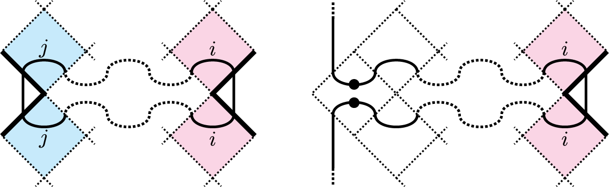
Corollary 6.17 The map
 $\vartheta $
is a
$\vartheta $
is a
 $\mathbb {Z}[q,q^{-1}]$
-module isomorphism.
$\mathbb {Z}[q,q^{-1}]$
-module isomorphism.
Proof Using Propositions 6.15 and 6.16, we have that every oriented Temperley–Lieb diagram
 $\lambda d \mu = \lambda \mathsf {e}_{\underline {w}} \mu = \mathsf {e}_{\mathsf {T}} = \vartheta (E_{\mathsf {T}})$
and so the map
$\lambda d \mu = \lambda \mathsf {e}_{\underline {w}} \mu = \mathsf {e}_{\mathsf {T}} = \vartheta (E_{\mathsf {T}})$
and so the map
 $\vartheta $
is surjective. To show that it is injective, note that the basis elements
$\vartheta $
is surjective. To show that it is injective, note that the basis elements
 $E_{\mathsf {T}}$
for
$E_{\mathsf {T}}$
for
 $\mathrm {TL}_{(W,P)}(q)$
given in Theorem 3.8 are mapped to distinct basis elements in
$\mathrm {TL}_{(W,P)}(q)$
given in Theorem 3.8 are mapped to distinct basis elements in
 $\mathrm {TL}^{\wedge \vee }_{(W,P)}(q)$
.
$\mathrm {TL}^{\wedge \vee }_{(W,P)}(q)$
.
This completes the proof of Theorem 6.12. From now on, we identify
 $\mathrm {TL}_{(W,P)}(q) = \mathrm {TL}^{\wedge \vee }_{(W,P)}(q)$
and use the diagrammatic notation for its elements.
$\mathrm {TL}_{(W,P)}(q) = \mathrm {TL}^{\wedge \vee }_{(W,P)}(q)$
and use the diagrammatic notation for its elements.
As noted earlier, if
 $\underline {w}$
and
$\underline {w}$
and
 $\underline {w}'$
are two reduced expressions for the same strongly fully commutative element w, then we have
$\underline {w}'$
are two reduced expressions for the same strongly fully commutative element w, then we have
 $\mathsf {e}_{\underline {w}} = \mathsf {e}_{\underline {w}'}$
. So we will denote this element by
$\mathsf {e}_{\underline {w}} = \mathsf {e}_{\underline {w}'}$
. So we will denote this element by
 $\mathsf {e}_w$
. In particular, for each
$\mathsf {e}_w$
. In particular, for each
 $\mu \in {^PW}$
we have the corresponding element
$\mu \in {^PW}$
we have the corresponding element
 $\mathsf {e}_\mu \in \mathrm {TL}_W(q)$
. (We will give a closed combinatorial description of this element in Section 8.) Now, restricting our attention to the anti-spherical module and using Corollary 3.10 gives the following.
$\mathsf {e}_\mu \in \mathrm {TL}_W(q)$
. (We will give a closed combinatorial description of this element in Section 8.) Now, restricting our attention to the anti-spherical module and using Corollary 3.10 gives the following.
Corollary 6.18 The anti-spherical module
 $\varnothing \mathrm {TL}_{(W,P)}(q)$
has basis given by
$\varnothing \mathrm {TL}_{(W,P)}(q)$
has basis given by
 $$\begin{align*}\{\mathsf{e}_{\mathsf{T}} = \varnothing \mathsf{e}_{\mu} \lambda \mid \mathsf{T} \in \mathrm{Path}(\lambda,\underline{\mu}), \lambda,\mu \in {^PW}\}.\end{align*}$$
In particular we have
 $$\begin{align*}|\mathrm{Path}(\lambda , \underline{\mu})|\leq 1\qquad \text{for all } \lambda, \mu \in {^PW}.\end{align*}$$
Thus, the diagrammatic oriented Temperley–Lieb algebra setting (and its anti-spherical module in particular) provides a diagrammatic model for studying the matrix
 $\Delta _{\lambda \mu }$
. More precisely, we have shown that
$\Delta _{\lambda \mu }$
. More precisely, we have shown that
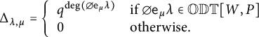 $$\begin{align*}\Delta_{\lambda,\mu}=\left\{ \begin{array}{ll} q^{\deg(\varnothing \mathsf{e}_\mu \lambda)} & \text{if } \varnothing \mathsf{e}_\mu \lambda\in \mathbb{ODT}[W,P]\\ 0 & \text{otherwise.}\end{array}\right. \end{align*}$$
In the next section, we investigate the degree of oriented Temperley–Lieb diagrams.
7 A closed combinatorial interpretation of the grading
The isomorphism
 $\vartheta $
given in Theorem 6.12 gives a grading on the diagrammatic oriented Temperley–Lieb algebra. Explicitly, we have that the degree of any oriented Temperley–Lieb diagram
$\vartheta $
given in Theorem 6.12 gives a grading on the diagrammatic oriented Temperley–Lieb algebra. Explicitly, we have that the degree of any oriented Temperley–Lieb diagram
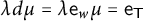 $\lambda d\mu = \lambda \mathsf {e}_w \mu = \mathsf {e}_{\mathsf {T}}$
is equal to
$\lambda d\mu = \lambda \mathsf {e}_w \mu = \mathsf {e}_{\mathsf {T}}$
is equal to
 $\deg (\mathsf {T})$
. This is computed as the sum of the degree of each step in the path
$\deg (\mathsf {T})$
. This is computed as the sum of the degree of each step in the path
 $\mathsf {T}$
. We now provide a closed combinatorial description of this degree in terms of the diagram
$\mathsf {T}$
. We now provide a closed combinatorial description of this degree in terms of the diagram
 $\lambda d \mu $
itself.
$\lambda d \mu $
itself.
Theorem 7.1 We define the degree of an oriented Temperley–Lieb diagram by assigning a degree to each of its strands and then summing over all strands. We define the degree of a northern arc whose rightmost vertex is labeled by
 $\vee $
to be
$\vee $
to be
 $+1$
, and the degree of a southern arc whose rightmost vertex is labeled by
$+1$
, and the degree of a southern arc whose rightmost vertex is labeled by
 $\wedge $
to be
$\wedge $
to be
 $-1$
. All other strands are defined to have degree
$-1$
. All other strands are defined to have degree
 $0$
(in particular, all propagating strands have degree
$0$
(in particular, all propagating strands have degree
 $0$
). Diagrammatically, we record the degree of an oriented Temperley–Lieb diagram as follows
$0$
). Diagrammatically, we record the degree of an oriented Temperley–Lieb diagram as follows
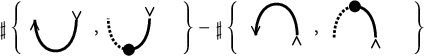
where the dots are to emphasise that the lefthand-side of the arc does not contribute to the degree. Then for any oriented Temperley–Lieb diagram
 $\lambda d \mu = \mathsf {e}_{\mathsf {T}}$
we have
$\lambda d \mu = \mathsf {e}_{\mathsf {T}}$
we have
 $\deg (\lambda d \mu ) = \deg (\mathsf {T})$
.
$\deg (\lambda d \mu ) = \deg (\mathsf {T})$
.
Proof We first check that the degree of the generators
 $\lambda \mathsf {e}_i \mu $
(for
$\lambda \mathsf {e}_i \mu $
(for
 $\mu = \lambda $
or
$\mu = \lambda $
or
 $\lambda s_i$
) are correct. Note that we have
$\lambda s_i$
) are correct. Note that we have
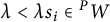 $\lambda < \lambda s_i\in {^PW}$
precisely when
$\lambda < \lambda s_i\in {^PW}$
precisely when
 $\lambda = \ldots \wedge \vee \ldots $
and
$\lambda = \ldots \wedge \vee \ldots $
and
 $\lambda s_i = \ldots \vee \wedge \ldots $
for
$\lambda s_i = \ldots \vee \wedge \ldots $
for
 $i\in \{1, \ldots n-1\}$
, or
$i\in \{1, \ldots n-1\}$
, or
 $\lambda = \vee \vee \ldots $
and
$\lambda = \vee \vee \ldots $
and
 $\lambda s_{1"} = \wedge \wedge \ldots $
, or
$\lambda s_{1"} = \wedge \wedge \ldots $
, or
 $\lambda = \circ \vee \ldots $
and
$\lambda = \circ \vee \ldots $
and
 $\lambda s_{1'} = \circ \wedge \ldots $
. So the degrees of the generators are given by
$\lambda s_{1'} = \circ \wedge \ldots $
. So the degrees of the generators are given by
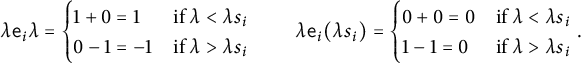 $$ \begin{align*}\lambda \mathsf{e}_ i \lambda = \begin{cases} 1+0=1 &\text{if } \lambda <\lambda s_i \\ 0-1=-1 &\text{if } \lambda>\lambda s_i \\ \end{cases} \qquad \lambda \mathsf{e}_ i (\lambda s_i) = \begin{cases} 0+0=0 &\text{if } \lambda <\lambda s_i \\ 1-1=0 &\text{if } \lambda>\lambda s_i \\ \end{cases}.\end{align*} $$
These are illustrated in Figure 20 for
 $i\in \{1, \ldots , n-1\}$
. Comparing these with Proposition 3.11 proves the result for the generators.
$i\in \{1, \ldots , n-1\}$
. Comparing these with Proposition 3.11 proves the result for the generators.
The four generators
 $\lambda \mathsf {e}_i \mu $
for
$\lambda \mathsf {e}_i \mu $
for
 $i\in \{1, \ldots n-1\}$
of degree
$i\in \{1, \ldots n-1\}$
of degree
 $1=1+0$
,
$1=1+0$
,
 $-1=0-1$
,
$-1=0-1$
,
 $0=0+0$
, and
$0=0+0$
, and
 $0=1-1,$
respectively. We record the degrees of the strand segments within the tile (with
$0=1-1,$
respectively. We record the degrees of the strand segments within the tile (with
 $+=1$
,
$+=1$
,
 $-=-1$
and
$-=-1$
and
 $\circ =0$
).
$\circ =0$
).
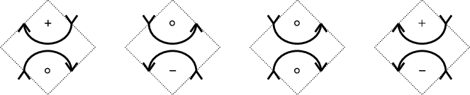
Now as explained in Subsection 6.3, we can write any oriented Temperley–Lieb diagram as a product of generators
 $\mathsf {e}_{\mathsf {T}}$
with
$\mathsf {e}_{\mathsf {T}}$
with
 $\omega (\mathsf {T})$
a reduced word for a strongly fully commutative element of W using a region in the tiling for W. Moreover, we have seen how each strand of the diagram corresponds to a horizontal strip in the tiling. We can then obtain the degree of strand in the product by adding the degree of each small arc coming from the generators. We now run through the various types of strands and check that the result holds in each case.
$\omega (\mathsf {T})$
a reduced word for a strongly fully commutative element of W using a region in the tiling for W. Moreover, we have seen how each strand of the diagram corresponds to a horizontal strip in the tiling. We can then obtain the degree of strand in the product by adding the degree of each small arc coming from the generators. We now run through the various types of strands and check that the result holds in each case.
First observe that any northern or southern arc passes through an odd number of tiles and any propagating strand passes through an even number of tiles. The undecorated northern arcs are illustrated in Figure 21.
The undecorated northern arcs.

In Figures 21-25, we highlight the tiles through which the strand “wiggles” and the degree of the strand within a given tile (which we have already calculated in terms of the generators. Note that, reading from left to right, the strand oscillates between being either the “top” or “bottom” of a given generator tile. Assume the arc is undecorated, northern, and clockwise-oriented. The degree contribution as the arc passes through these tiles is given by
 $$ \begin{align*} +1 -1 +1-1+1-1\dots +1=1 \end{align*} $$
(notice that the strand is locally either a clockwise northern arc or an anticlockwise southern arc at each step). If an undecorated northern arc is anti-clockwise oriented then it has degree
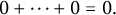 $$ \begin{align*}0+\dots+0=0. \end{align*} $$
Thus the degrees match up. The degrees of undecorated southern arcs can be computed similarly. The degree of undecorated propagating strands can easily be seen to be zero as illustrated in Figure 24.
Degree 1 decorated northern strands. The pink highlights an odd number of boxes, the blue highlights an even number. In this way, note that the blue section of the strand never contributes to the degree, regardless of the orientation.

Degree zero decorated northern strands.

The decorated northern arcs of degree 1 in type
 $(C_{n-1}, A_{n-2})$
are illustrated in Figures 22–25. Swapping the orientation of the rightmost vertex from
$(C_{n-1}, A_{n-2})$
are illustrated in Figures 22–25. Swapping the orientation of the rightmost vertex from
 $\vee $
to
$\vee $
to
 $\wedge $
, we see that the pink strip now doesn’t contribute to the degree either, and so these northern arc have degree zero. The decorated southern arcs can be dealt with in a similar way.
$\wedge $
, we see that the pink strip now doesn’t contribute to the degree either, and so these northern arc have degree zero. The decorated southern arcs can be dealt with in a similar way.
The undecorated propagating strands, all of which are of degree
 $0$
.
$0$
.

The decorated propagating strands, all of which are of degree
 $0$
.
$0$
.
It is easy to see that any (decorated) propagating strand also has degree zero as it goes through an even number of tiles.
Finally, the strands in a diagram of type
 $(D_n, A_{n-1})$
are the same as those in type
$(D_n, A_{n-1})$
are the same as those in type
 $(C_{n-1}, A_{n-2})$
except that they contain at most one decoration and we only need to consider arcs which are flip-oriented. So the result holds for these as well.
$(C_{n-1}, A_{n-2})$
except that they contain at most one decoration and we only need to consider arcs which are flip-oriented. So the result holds for these as well.
Corollary 7.2 The anti-spherical module for
 $\mathrm {TL}_{(W,P)}(q)$
is non-negatively graded, that is
$\mathrm {TL}_{(W,P)}(q)$
is non-negatively graded, that is
 $$ \begin{align*}\deg(\varnothing \mathsf{e}_{\mu} \lambda ) \geq 0 \qquad \text{for all } \lambda ,\mu \in {^PW}.\end{align*} $$
Thus, the non-zero entries in the light leaves matrix
 $\Delta _{\lambda ,\mu }$
are non-negative powers of q.
$\Delta _{\lambda ,\mu }$
are non-negative powers of q.
Proof Any northern arc or propagating strand is non-negatively graded, thus it suffices to consider the southern arcs (which can be negatively graded). Now recall the coset diagram for
 $\varnothing $
in types
$\varnothing $
in types
 $(W,P)=(A_n,A_{k}\times A_{n-k-1})$
,
$(W,P)=(A_n,A_{k}\times A_{n-k-1})$
,
 $(C_n,A_{n-1})$
,
$(C_n,A_{n-1})$
,
 $(D_{n},A_{n-1})$
from Section 5. We see that any southern arc must have rightmost vertex labeled by
$(D_{n},A_{n-1})$
from Section 5. We see that any southern arc must have rightmost vertex labeled by
 $\vee $
. So the southern arcs all have degree zero. This proves the result.
$\vee $
. So the southern arcs all have degree zero. This proves the result.
8 Factorization of the light leaves matrix
We now explain how to construct the element
 $\mathsf {e}_\mu \in \mathrm {TL}_W(q)$
for
$\mathsf {e}_\mu \in \mathrm {TL}_W(q)$
for
 $\mu \in {^PW}$
via an efficient closed combinatorial algorithm, which has its origins in [Reference Brundan and StroppelBS12, Reference Cox and De VisscherCD11, Reference Ehrig and StroppelES16b, Reference MartinMar15]. This allows us to enumerate the elements
$\mu \in {^PW}$
via an efficient closed combinatorial algorithm, which has its origins in [Reference Brundan and StroppelBS12, Reference Cox and De VisscherCD11, Reference Ehrig and StroppelES16b, Reference MartinMar15]. This allows us to enumerate the elements
 $\varnothing \mathsf {e}_\mu \lambda $
and hence the paths
$\varnothing \mathsf {e}_\mu \lambda $
and hence the paths
 $\mathrm {NPath} (\lambda ,\underline {\mu }) \subseteq \mathrm {Path} (\lambda ,\underline {\mu })$
and
$\mathrm {NPath} (\lambda ,\underline {\mu }) \subseteq \mathrm {Path} (\lambda ,\underline {\mu })$
and
 $ \mathrm {BPath} (\nu ,\underline {\mu }) \subseteq \mathrm {Path} (\nu ,\underline {\mu })$
corresponding to decomposition numbers and bases of simple modules for the Hecke category respectively (in other words, solving Libedinsky–Williamson’s question for Hermitian symmetric pairs).
$ \mathrm {BPath} (\nu ,\underline {\mu }) \subseteq \mathrm {Path} (\nu ,\underline {\mu })$
corresponding to decomposition numbers and bases of simple modules for the Hecke category respectively (in other words, solving Libedinsky–Williamson’s question for Hermitian symmetric pairs).
We have seen that every strongly fully commutative element w in W with
 $\underline {w} = \omega (\mathsf {T})$
for some
$\underline {w} = \omega (\mathsf {T})$
for some
 $\mathsf {T}\in \mathrm {Path}_{(W,P)}$
corresponds to a region
$\mathsf {T}\in \mathrm {Path}_{(W,P)}$
corresponds to a region
 $R(w)$
in the tiling of W. That region is determined by the path
$R(w)$
in the tiling of W. That region is determined by the path
 $\pi (w)$
walking along its boundary, starting with its northern boundary going East and coming back along its southern boundary going West. When
$\pi (w)$
walking along its boundary, starting with its northern boundary going East and coming back along its southern boundary going West. When
 $w=\mu \in {^PW}$
, the region
$w=\mu \in {^PW}$
, the region
 $R(\mu )$
has a particularly simple shape.
$R(\mu )$
has a particularly simple shape.
Lemma 8.1 We have that
 $w\in {^PW}$
if and only if the region
$w\in {^PW}$
if and only if the region
 $R(w)$
has the following property. In type
$R(w)$
has the following property. In type
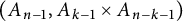 $(A_{n-1}, A_{k-1}\times A_{n-k-1})$
, the last n steps of the path
$(A_{n-1}, A_{k-1}\times A_{n-k-1})$
, the last n steps of the path
 $\pi (w)$
are given by
$\pi (w)$
are given by
 $((SW)^{n-k}, (NW)^{k})$
. In types
$((SW)^{n-k}, (NW)^{k})$
. In types
 $(C_{n-1},A_{n-2})$
and
$(C_{n-1},A_{n-2})$
and
 $(D_n, A_{n-1})$
, the last n steps of the path
$(D_n, A_{n-1})$
, the last n steps of the path
 $\pi (w)$
are given by
$\pi (w)$
are given by
 $((SW)^n)$
.
$((SW)^n)$
.
Proof Note that the minimal length coset representatives
 $\mu \in {^PW}$
are characterised by the fact that every reduced expression for
$\mu \in {^PW}$
are characterised by the fact that every reduced expression for
 $\mu $
starts with
$\mu $
starts with
 $s\notin P$
. From that characterisation, it is clear that if
$s\notin P$
. From that characterisation, it is clear that if
 $\pi (w)$
has the stated form then
$\pi (w)$
has the stated form then
 $w\in {^PW}$
. Examples of
$w\in {^PW}$
. Examples of
 $\pi (\mu )$
for
$\pi (\mu )$
for
 $\mu \in {^PW}$
are given in the first two pictures in Figures 16 and 17. Now suppose that
$\mu \in {^PW}$
are given in the first two pictures in Figures 16 and 17. Now suppose that
 $\pi (w)$
does not have the stated form then
$\pi (w)$
does not have the stated form then
 $\pi (w)$
would have two consecutive steps
$\pi (w)$
would have two consecutive steps
 $\pi ((n-i)') = SW$
and
$\pi ((n-i)') = SW$
and
 $\pi ((n-i-1)') = NW$
(with
$\pi ((n-i-1)') = NW$
(with
 $i\neq k$
in type
$i\neq k$
in type
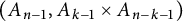 $(A_{n-1}, A_{k-1}\times A_{n-k-1})$
). But this would imply that there is a reduced expression for w starting with some
$(A_{n-1}, A_{k-1}\times A_{n-k-1})$
). But this would imply that there is a reduced expression for w starting with some
 $s\in P$
and so
$s\in P$
and so
 $w\notin {^PW}$
. This is illustrated in the rightmost picture of Figures 16 and 17 where we indeed observe that there is a reduced word for w starting with
$w\notin {^PW}$
. This is illustrated in the rightmost picture of Figures 16 and 17 where we indeed observe that there is a reduced word for w starting with ![]() in each case.
in each case.
Therefore for
 $\mu \in {^PW}$
, the region
$\mu \in {^PW}$
, the region
 $R(\mu )$
is completely determined by its northern boundary. In fact, we have the following natural correspondence between the northern boundary of
$R(\mu )$
is completely determined by its northern boundary. In fact, we have the following natural correspondence between the northern boundary of
 $R(\mu )$
and the coset diagram of
$R(\mu )$
and the coset diagram of
 $\mu $
.
$\mu $
.
Lemma 8.2 Let
 $\mu \in {^PW}$
. The i-th vertex of the coset diagram of
$\mu \in {^PW}$
. The i-th vertex of the coset diagram of
 $\mu $
is labeled by
$\mu $
is labeled by
 $\wedge $
, respectively
$\wedge $
, respectively
 $\vee $
, if and only if the i-th step in
$\vee $
, if and only if the i-th step in
 $\pi (\mu )$
is given by
$\pi (\mu )$
is given by
 $SE$
, respectively,
$SE$
, respectively,
 $NE$
. In type
$NE$
. In type
 $(C_{n-1}, A_{n-2}),$
the first vertex is always labeled by
$(C_{n-1}, A_{n-2}),$
the first vertex is always labeled by
 $\circ $
and the first step is always
$\circ $
and the first step is always
 $SE$
.
$SE$
.
Proof We proceed by induction on
 $\ell (\mu )$
. For
$\ell (\mu )$
. For
 $\ell (\mu ) = 0,$
we have
$\ell (\mu ) = 0,$
we have
 $\mu = \varnothing $
and the result is clear from the description of the coset diagram for
$\mu = \varnothing $
and the result is clear from the description of the coset diagram for
 $\varnothing $
given in Section 5. Now assume that the result holds for
$\varnothing $
given in Section 5. Now assume that the result holds for
 $\lambda \in {^PW}$
and let
$\lambda \in {^PW}$
and let
 $\mu = \lambda s_i> \lambda $
. If
$\mu = \lambda s_i> \lambda $
. If
 $i=1, \ldots , n-1$
then the coset diagrams for
$i=1, \ldots , n-1$
then the coset diagrams for
 $\lambda $
and
$\lambda $
and
 $\lambda s_i$
only differ in position i and
$\lambda s_i$
only differ in position i and
 $i+1$
and we have
$i+1$
and we have
 $\lambda = \ldots \wedge \vee \ldots $
and
$\lambda = \ldots \wedge \vee \ldots $
and
 $\lambda s_i = \ldots \vee \wedge \ldots $
. The corresponding paths
$\lambda s_i = \ldots \vee \wedge \ldots $
. The corresponding paths
 $\pi (\lambda )$
and
$\pi (\lambda )$
and
 $\pi (\lambda s_i)$
are depicted in Figure 26. We see that the i-th and
$\pi (\lambda s_i)$
are depicted in Figure 26. We see that the i-th and
 $(i+1)$
-th steps in
$(i+1)$
-th steps in
 $\lambda $
, respectively
$\lambda $
, respectively
 $\lambda s_i$
, are given by
$\lambda s_i$
, are given by
 $SE, NE$
, respectively,
$SE, NE$
, respectively,
 $NE, SE$
and so the result follows by induction. For
$NE, SE$
and so the result follows by induction. For
 $i=1'$
, the coset diagrams of
$i=1'$
, the coset diagrams of
 $\lambda $
and
$\lambda $
and
 $\lambda s_{1'}$
only differ in the second position and we have
$\lambda s_{1'}$
only differ in the second position and we have
 $\lambda = \circ \vee \ldots $
and
$\lambda = \circ \vee \ldots $
and
 $\lambda s_{1'} = \circ \wedge \ldots $
. The corresponding paths
$\lambda s_{1'} = \circ \wedge \ldots $
. The corresponding paths
 $\pi (\lambda )$
and
$\pi (\lambda )$
and
 $\pi (\lambda s_{1'})$
are depicted in Figure 26. We see that the second step in
$\pi (\lambda s_{1'})$
are depicted in Figure 26. We see that the second step in
 $\lambda $
is given by
$\lambda $
is given by
 $NE$
while the second step in
$NE$
while the second step in
 $\lambda s_{1'}$
is given by
$\lambda s_{1'}$
is given by
 $SE$
, and so the result follows by induction. Finally, if
$SE$
, and so the result follows by induction. Finally, if
 $i=1"$
then the coset diagrams for
$i=1"$
then the coset diagrams for
 $\lambda $
and
$\lambda $
and
 $\lambda s_{1"}$
only different in the first two positions and we have
$\lambda s_{1"}$
only different in the first two positions and we have
 $\lambda = \vee \vee \ldots $
and
$\lambda = \vee \vee \ldots $
and
 $\lambda s_{1"} = \wedge \wedge \ldots $
. The corresponding paths
$\lambda s_{1"} = \wedge \wedge \ldots $
. The corresponding paths
 $\pi (\lambda )$
and
$\pi (\lambda )$
and
 $\pi (\lambda s_{1"})$
are depicted in Figure 26. We see that the first two steps in
$\pi (\lambda s_{1"})$
are depicted in Figure 26. We see that the first two steps in
 $\lambda $
, respectively
$\lambda $
, respectively
 $\lambda s_{1"}$
, are given by
$\lambda s_{1"}$
, are given by
 $NE,NE$
, respectively
$NE,NE$
, respectively
 $SE, SE$
, and so the result follows by induction.
$SE, SE$
, and so the result follows by induction.
The effect of applying a reflection ![]() for
for
 $1\leq i \leq n-1$
; the reflection
$1\leq i \leq n-1$
; the reflection ![]() (in type C); and the reflection
(in type C); and the reflection ![]() (in type D) respectively. In each case, we depict the pair of weights
(in type D) respectively. In each case, we depict the pair of weights
 $\lambda $
and
$\lambda $
and ![]() and the corresponding northern edges of the paths
and the corresponding northern edges of the paths
 $\pi (\lambda )$
and
$\pi (\lambda )$
and ![]() . We highlight in blue and pink the difference between
. We highlight in blue and pink the difference between
 $\lambda $
and
$\lambda $
and ![]() (both on the level of tiles and coset diagrams).
(both on the level of tiles and coset diagrams).

Using this correspondence, we easily obtain the following closed combinatorial algorithm to construct
 $\mathsf {e}_{\mu }$
.
$\mathsf {e}_{\mu }$
.
Proposition 8.3 For each
 $\mu \in {^PW}$
, the diagram
$\mu \in {^PW}$
, the diagram
 $\mathsf {e}_\mu \in \mathrm {TL}_W(q)$
can be constructed as follows. Place the coset diagram
$\mathsf {e}_\mu \in \mathrm {TL}_W(q)$
can be constructed as follows. Place the coset diagram
 $\mu $
on the northern boundary and
$\mu $
on the northern boundary and
 $\varnothing $
on the southern boundary. Then
$\varnothing $
on the southern boundary. Then
-
(1) Repeatedly connect neighbouring northern vertices (in the sense that they are next to each other or only have vertices already connected by an arc between them) labeled by
$\vee $
and
$\wedge $
by a northern anti-clockwise arc.We are left with (in type
$(C_{n-1}, A_{n-2})$
one vertex labeled by
$\circ $
followed by) some vertices labeled by
$\wedge $
followed by some vertices labeled by
$\vee $
. - (2)
-
(a) In type
$(A_{n-1}, A_{k-1}\times A_{n-k-1})$
, draw undecorated propagating strands on all remaining vertices. -
(b) In type
$(D_n, A_{n-1})$
, starting from the left, connect neighbouring vertices labeled with
$\wedge $
’s with decorated northern arcs. Then draw a decorated propagating strand from the remaining vertex labeled by
$\wedge $
(if it exists), and undecorated propagating strands on all remaining vertices labeled by
$\vee $
. -
(c) In type
$(C_{n-1}, A_{n-2})$
, if
$\mu = \varnothing $
, then draw an undecorated propagating strand from each northern vertex. Otherwise, view the first label
$\circ $
of
$\mu $
as a
$\wedge $
, then follow exactly the same procedure as in type
$(D_n, A_{n-1})$
.
-


Now there is a unique way of completing the diagram
 $\mathsf {e}_\mu $
such that
$\mathsf {e}_\mu $
such that
 $\varnothing \mathsf {e}_\mu \mu \in \mathbb {ODT}[W,P]$
.
$\varnothing \mathsf {e}_\mu \mu \in \mathbb {ODT}[W,P]$
.
Example 8.4 A couple of illustrative large examples of the construction in Proposition 8.3 are given in Figures 27 and 28. The complete set of all
 $\mathsf {e}_\mu $
for
$\mathsf {e}_\mu $
for
 $\mu \in {^PW}$
for
$\mu \in {^PW}$
for
 $(W,P)$
of type
$(W,P)$
of type
 $(D_4 , A_3)$
and
$(D_4 , A_3)$
and
 $(C_3 , A_2)$
are given in Figure 29. In all examples, we will only picture the top of the diagram as this completely determines
$(C_3 , A_2)$
are given in Figure 29. In all examples, we will only picture the top of the diagram as this completely determines
 $\mathsf {e}_\mu $
.
$\mathsf {e}_\mu $
.
Two examples of the construction of
 $\mathsf {e}_\mu $
, the former is of type
$\mathsf {e}_\mu $
, the former is of type
 $(A_8, A_4\times A_3)$
and the latter is of type
$(A_8, A_4\times A_3)$
and the latter is of type
 $(C_8, A_7)$
.
$(C_8, A_7)$
.
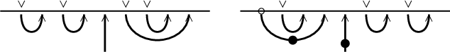
An example of the construction of
 $\mathsf {e}_\mu $
in type
$\mathsf {e}_\mu $
in type
 $(D_{19},A_{18})$
.
$(D_{19},A_{18})$
.

The construction of
 $\mathsf {e}_\mu $
for all
$\mathsf {e}_\mu $
for all
 $\mu \in {^PW}$
in types
$\mu \in {^PW}$
in types
 $(D_4 , A_3)$
and
$(D_4 , A_3)$
and
 $(C_3 , A_2)$
.
$(C_3 , A_2)$
.
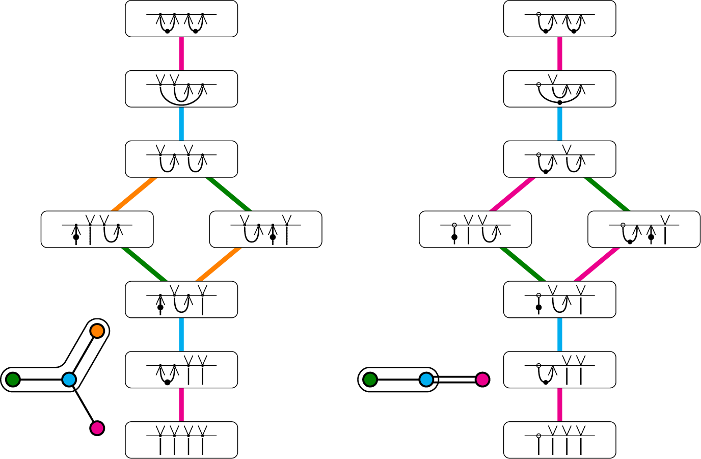
Proposition 8.3 gives us an efficient way of finding the degree of
 $\varnothing \mathsf {e}_\mu \lambda $
as the number of northern arcs whose rightmost vertex is labeled by
$\varnothing \mathsf {e}_\mu \lambda $
as the number of northern arcs whose rightmost vertex is labeled by
 $\vee $
. As this does not depend on the bottom of the diagram (as all southern arcs have degree zero), we will only depict the top of
$\vee $
. As this does not depend on the bottom of the diagram (as all southern arcs have degree zero), we will only depict the top of
 $\varnothing \mathsf {e}_\mu \lambda $
. Examples are given in Figures 30 and 31.
$\varnothing \mathsf {e}_\mu \lambda $
. Examples are given in Figures 30 and 31.
The elements
 $\varnothing \mathsf {e}_\mu \lambda $
from the first column of Figure 31 in order.
$\varnothing \mathsf {e}_\mu \lambda $
from the first column of Figure 31 in order.

The
 $q^{\deg ({{\varnothing \mathsf {e}_\mu \lambda }})}$
for
$q^{\deg ({{\varnothing \mathsf {e}_\mu \lambda }})}$
for
 $\lambda ,\mu \in {{^P}W}$
for
$\lambda ,\mu \in {{^P}W}$
for
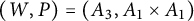 $(W,P)= (A_3,A_1\times A_1)$
.
$(W,P)= (A_3,A_1\times A_1)$
.
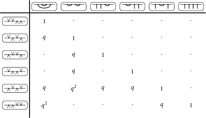
We have already seen in Corollary 7.2 that the entries in the light leaves matrix
 $\Delta _{\lambda \mu }$
are either zero or non-negative powers of q. In the simply-laced cases, we can say more.
$\Delta _{\lambda \mu }$
are either zero or non-negative powers of q. In the simply-laced cases, we can say more.
Theorem 8.5 Assume
 $(W,P)=(A_{n-1}, A_{n-2})$
or
$(W,P)=(A_{n-1}, A_{n-2})$
or
 $(D_n, A_{n-1})$
. Then for any
$(D_n, A_{n-1})$
. Then for any
 $\lambda , \mu \in {^PW}$
with
$\lambda , \mu \in {^PW}$
with
 $\varnothing \mathsf {e}_\mu \lambda \in \mathbb {ODT}[W,P],$
we have
$\varnothing \mathsf {e}_\mu \lambda \in \mathbb {ODT}[W,P],$
we have
 $\deg (\varnothing \mathsf { e}_\mu \lambda ) = 0$
if and only if
$\deg (\varnothing \mathsf { e}_\mu \lambda ) = 0$
if and only if
 $\lambda = \mu $
. In particular, we have
$\lambda = \mu $
. In particular, we have
 $\Delta _{\lambda \mu } = 1$
if and only if
$\Delta _{\lambda \mu } = 1$
if and only if
 $\lambda = \mu $
and so the matrix of light leaves has a trivial factorization
$\lambda = \mu $
and so the matrix of light leaves has a trivial factorization
 $$ \begin{align*}B = \mathrm{Id} \quad \text{and} \quad \Delta = N .\end{align*} $$
Proof Fix
 $\mu \in {^PW}$
and consider all
$\mu \in {^PW}$
and consider all
 $\lambda \in {^PW}$
with
$\lambda \in {^PW}$
with
 $\varnothing \mathsf {e}_\mu \lambda \in \mathbb {ODT}[W,P]$
and
$\varnothing \mathsf {e}_\mu \lambda \in \mathbb {ODT}[W,P]$
and
 $\deg (\varnothing \mathsf {e}_\mu \lambda ) = 0$
. Note that this forces all undecorated northern arcs to be anti-clockwise, all undecorated propagating strands to be oriented, all northern decorated arcs to be labeled by two
$\deg (\varnothing \mathsf {e}_\mu \lambda ) = 0$
. Note that this forces all undecorated northern arcs to be anti-clockwise, all undecorated propagating strands to be oriented, all northern decorated arcs to be labeled by two
 $\wedge $
’s and all decorated propagating strands to be flip-oriented. This gives only one choice for
$\wedge $
’s and all decorated propagating strands to be flip-oriented. This gives only one choice for
 $\lambda $
, namely
$\lambda $
, namely
 $\lambda = \mu $
.
$\lambda = \mu $
.
Thus, setting every basis element
 $\varnothing \mathsf {e}_\mu \lambda $
for the anti-spherical module to be standard proves Theorem A in type
$\varnothing \mathsf {e}_\mu \lambda $
for the anti-spherical module to be standard proves Theorem A in type
 $(W,P)=(A_{n-1}, A_{n-2})$
and
$(W,P)=(A_{n-1}, A_{n-2})$
and
 $(D_n, A_{n-1})$
. We now state and proof Theorem A in the only remaining type of Hermitian symmetric pair, namely
$(D_n, A_{n-1})$
. We now state and proof Theorem A in the only remaining type of Hermitian symmetric pair, namely
 $(C_{n}, A_{n-1})$
.
$(C_{n}, A_{n-1})$
.
Theorem 8.6 Let
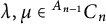 $\lambda , \mu \in {^{A_{n-1}}C_{n}}$
. We say that
$\lambda , \mu \in {^{A_{n-1}}C_{n}}$
. We say that
 $\varnothing \mathsf {e}_{\mu } \lambda \in \mathbb {ODT}[C_n, A_{n-1}]$
is
standard
if every decorated strand if flip-oriented.
$\varnothing \mathsf {e}_{\mu } \lambda \in \mathbb {ODT}[C_n, A_{n-1}]$
is
standard
if every decorated strand if flip-oriented.
We define the matrices N and B in type
 $(W,P)=(C_n, A_{n-1})$
as follows:
$(W,P)=(C_n, A_{n-1})$
as follows:
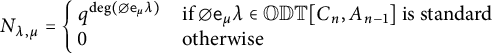 $$ \begin{align} N_{ \lambda,\mu} &= \left\{\!\! \begin{array}{ll} q^{\deg (\varnothing \mathsf{e}_{\mu} \lambda)} & \text{if } \varnothing \mathsf{e}_\mu \lambda \in \mathbb{ODT}[C_n, A_{n-1}] \text{ is standard}\\ 0 & \text{otherwise} \end{array}\right. \end{align} $$
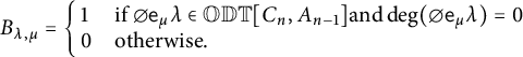 $$ \begin{align} B_{ \lambda,\mu} &= \left\{\!\! \begin{array}{ll} 1 & \text{if } \varnothing \mathsf{e}_\mu \lambda\in \mathbb{ODT}[C_{n}, A_{n-1}] \text{and} \deg (\varnothing \mathsf{e}_\mu \lambda) =0\\ 0 & \text{otherwise.} \end{array}\right. \end{align} $$
Then the matrix of light leaves in type
 $(C_n, A_{n-1})$
factorizes as
$(C_n, A_{n-1})$
factorizes as
 $$ \begin{align*}\Delta = N B.\end{align*} $$
Proof Fix
 $\mu \in {^{A_{n-1}}C_n}$
and consider
$\mu \in {^{A_{n-1}}C_n}$
and consider
 $$ \begin{align*}C_\mu = \{\lambda \in {^{A_{n-1}}C_n} \, : \, \varnothing \mathsf{e}_\mu \lambda \in \mathbb{ODT}[C_n, A_{n-1}] \}.\end{align*} $$
Define an equivalence relation on
 $C_\mu $
by setting
$C_\mu $
by setting
 $\lambda \sim _\mu \eta $
for
$\lambda \sim _\mu \eta $
for
 $\lambda , \eta \in C_\mu $
if
$\lambda , \eta \in C_\mu $
if
 $\varnothing \mathsf {e}_\mu \lambda $
and
$\varnothing \mathsf {e}_\mu \lambda $
and
 $\varnothing \mathsf {e}_\mu \eta $
differ only in one northern arc where the differing arcs are given by
$\varnothing \mathsf {e}_\mu \eta $
differ only in one northern arc where the differing arcs are given by

We extend
 $\sim _{\mu }$
by transitivity. Note that, under this relation, each equivalence class contains a unique element
$\sim _{\mu }$
by transitivity. Note that, under this relation, each equivalence class contains a unique element
 $\nu $
satisfying
$\nu $
satisfying
 $\deg (\varnothing \mathsf {e}_\mu \nu ) = 0$
(obtained by orienting all northern arcs with rightmost vertex labeled by
$\deg (\varnothing \mathsf {e}_\mu \nu ) = 0$
(obtained by orienting all northern arcs with rightmost vertex labeled by
 $\wedge $
).
$\wedge $
).
Now, let
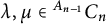 $\lambda , \mu \in {^{A_{n-1}}C_n}$
. We claim that
$\lambda , \mu \in {^{A_{n-1}}C_n}$
. We claim that
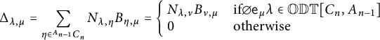 $$ \begin{align*}\Delta_{\lambda , \mu} = \sum_{\eta \in {^{A_{n-1}}C_n}} N_{\lambda , \eta} B_{\eta, \mu} = \left\{\!\! \begin{array}{ll} N_{\lambda , \nu} B_{\nu, \mu} & \text{if} \varnothing \mathsf{e}_\mu \lambda \in \mathbb{ODT}[C_n, A_{n-1}] \\ 0 & \text{otherwise} \end{array}\right.\end{align*} $$
where
 $\nu $
is the unique element satisfying
$\nu $
is the unique element satisfying
 $\lambda \sim _\mu \nu $
and
$\lambda \sim _\mu \nu $
and
 $\deg (\varnothing \mathsf {e}_\mu \nu ) =0$
. Suppose that
$\deg (\varnothing \mathsf {e}_\mu \nu ) =0$
. Suppose that
 $N_{\lambda , \eta } \neq 0$
and
$N_{\lambda , \eta } \neq 0$
and
 $B_{\eta , \mu }\neq 0$
for some
$B_{\eta , \mu }\neq 0$
for some
 $\eta $
. This implies that
$\eta $
. This implies that
 $\varnothing \mathsf {e}_\mu \eta \in \mathbb {ODT}[C_n, A_{n-1}]$
with
$\varnothing \mathsf {e}_\mu \eta \in \mathbb {ODT}[C_n, A_{n-1}]$
with
 $\deg (\varnothing \mathsf {e}_\mu \eta ) = 0$
, that is all northern arcs in
$\deg (\varnothing \mathsf {e}_\mu \eta ) = 0$
, that is all northern arcs in
 $\varnothing \mathsf {e}_\mu \eta $
have rightmost vertex labeled by
$\varnothing \mathsf {e}_\mu \eta $
have rightmost vertex labeled by
 $\wedge $
. Thus we have that
$\wedge $
. Thus we have that
 $\mathsf {e}_{\eta }$
has the same arcs as
$\mathsf {e}_{\eta }$
has the same arcs as
 $\mathsf {e}_\mu $
but with beads corresponding to oriented decorated northern arcs not connected to the symbol
$\mathsf {e}_\mu $
but with beads corresponding to oriented decorated northern arcs not connected to the symbol
 $\circ $
in
$\circ $
in
 $\varnothing \mathsf {e}_\mu \eta $
removed. Now,
$\varnothing \mathsf {e}_\mu \eta $
removed. Now,
 $N_{\lambda , \eta }\neq 0$
means that
$N_{\lambda , \eta }\neq 0$
means that
 $\varnothing \mathsf {e}_{\eta }\lambda \in \mathbb {ODT}[C_{n}, A_{n-1}]$
is standard. This implies that we also have
$\varnothing \mathsf {e}_{\eta }\lambda \in \mathbb {ODT}[C_{n}, A_{n-1}]$
is standard. This implies that we also have
 $\varnothing \mathsf {e}_\mu \lambda \in \mathbb {ODT}[C_n, A_{n-1}]$
. Now we claim, we have
$\varnothing \mathsf {e}_\mu \lambda \in \mathbb {ODT}[C_n, A_{n-1}]$
. Now we claim, we have
 $\lambda \sim _\mu \eta $
. The fact that the northern arcs are related as in (8.3) follows by definition. That the orientation of the propagating lines of
$\lambda \sim _\mu \eta $
. The fact that the northern arcs are related as in (8.3) follows by definition. That the orientation of the propagating lines of
 $\varnothing \mathsf {e}_\mu \lambda $
and
$\varnothing \mathsf {e}_\mu \lambda $
and
 $\varnothing \mathsf {e}_\mu \eta $
coincide follows from the fact that the orientation on the southern boundary is given by
$\varnothing \mathsf {e}_\mu \eta $
coincide follows from the fact that the orientation on the southern boundary is given by
 $\varnothing $
in both cases and if
$\varnothing $
in both cases and if
 $\mathsf {e}_\mu $
contains a decorated propagating line then its northern label is given by the parity condition. Now as
$\mathsf {e}_\mu $
contains a decorated propagating line then its northern label is given by the parity condition. Now as
 $\eta \sim _\mu \lambda $
and
$\eta \sim _\mu \lambda $
and
 $\deg (\varnothing \mathsf {e}_\mu \eta ) = 0$
implies that
$\deg (\varnothing \mathsf {e}_\mu \eta ) = 0$
implies that
 $\eta = \nu $
. Thus we have shown that
$\eta = \nu $
. Thus we have shown that
 $$ \begin{align*}\sum_{\eta \in {^{A_{n-1}}C_n}} N_{\lambda , \eta}B_{\eta , \mu} = N_{\lambda , \nu} B_{\nu, \mu}.\end{align*} $$
Finally note that, as
 $\nu \sim _{\mu } \lambda $
, a decorated arc in
$\nu \sim _{\mu } \lambda $
, a decorated arc in
 $\mathsf {e}_\mu $
is oriented in
$\mathsf {e}_\mu $
is oriented in
 $\varnothing \mathsf {e}_\mu \lambda $
if and only if it is oriented in
$\varnothing \mathsf {e}_\mu \lambda $
if and only if it is oriented in
 $\varnothing \mathsf {e}_\mu \nu $
. Now, as noted above,
$\varnothing \mathsf {e}_\mu \nu $
. Now, as noted above,
 $\mathsf {e}_\nu $
is obtained from
$\mathsf {e}_\nu $
is obtained from
 $\mathsf {e}_\mu $
by removing all beads on these oriented decorated arcs but the position of the arcs are the same and so
$\mathsf {e}_\mu $
by removing all beads on these oriented decorated arcs but the position of the arcs are the same and so
 $\deg ( \varnothing \mathsf {e}_\mu \lambda ) = \deg (\varnothing \mathsf {e}_\nu \lambda )$
. Thus we get
$\deg ( \varnothing \mathsf {e}_\mu \lambda ) = \deg (\varnothing \mathsf {e}_\nu \lambda )$
. Thus we get
 $$ \begin{align*}\Delta_{\lambda , \mu} = q^{\deg (\varnothing \mathsf{e}_\mu \lambda)} = q^{\deg ( \varnothing \mathsf{e}_\nu \lambda)} = N_{\lambda , \nu}B_{\nu , \mu}.\end{align*} $$
as required.
Remark 8.7 Note that the unique element
 $\nu $
described in the proof above is precisely the element satisfying
$\nu $
described in the proof above is precisely the element satisfying
 $\varphi (\varnothing \mathsf {e}_\mu \lambda ) = \overline {\varnothing } \mathsf {e}_{\overline {\nu }}\overline {\lambda }$
where
$\varphi (\varnothing \mathsf {e}_\mu \lambda ) = \overline {\varnothing } \mathsf {e}_{\overline {\nu }}\overline {\lambda }$
where
 $\varphi : \mathrm {TL}_{(C_n, A_{n-1})}(q) \rightarrow \mathrm {TL}_{(D_{n+1}, A_n)}(q)$
is the homomorphism defined in Proposition 6.11.
$\varphi : \mathrm {TL}_{(C_n, A_{n-1})}(q) \rightarrow \mathrm {TL}_{(D_{n+1}, A_n)}(q)$
is the homomorphism defined in Proposition 6.11.
Example 8.8 There are 6 non-standard basis elements
 $\varnothing \mathsf {e}_\mu \lambda $
in the anti-spherical module of type
$\varnothing \mathsf {e}_\mu \lambda $
in the anti-spherical module of type
 $(C_3,A_2)$
(this can be deduced from Example 2.3 and Theorem 8.6), these are depicted in Figure 32.
$(C_3,A_2)$
(this can be deduced from Example 2.3 and Theorem 8.6), these are depicted in Figure 32.
The six non-standard diagrams of type
 $(C_3,A_2)$
. The first and third of these diagrams have degree zero.
$(C_3,A_2)$
. The first and third of these diagrams have degree zero.
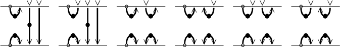
Corollary 8.9 Under the parity specialisation map
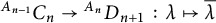 ${^{A_{n-1}}C_n} \rightarrow {^{A_n}D_{n+1}}\, : \, \lambda \mapsto \overline {\lambda }$
given in Definition 6.10 we have that
${^{A_{n-1}}C_n} \rightarrow {^{A_n}D_{n+1}}\, : \, \lambda \mapsto \overline {\lambda }$
given in Definition 6.10 we have that
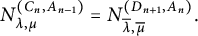 $$ \begin{align*}N^{(C_n, A_{n-1})}_{\lambda , \mu} = N^{(D_{n+1}, A_n)}_{\overline{\lambda}, \overline{\mu}}.\end{align*} $$
Proof We need to show that
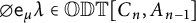 $\varnothing \mathsf {e}_\mu \lambda \in \mathbb {ODT}[C_n, A_{n-1}]$
is standard if and only if
$\varnothing \mathsf {e}_\mu \lambda \in \mathbb {ODT}[C_n, A_{n-1}]$
is standard if and only if
 $\overline {\varnothing } \mathsf {e}_{\overline {\mu }} \overline {\lambda }\in \mathbb {ODT}[D_{n+1}, A_n]$
. First note that if
$\overline {\varnothing } \mathsf {e}_{\overline {\mu }} \overline {\lambda }\in \mathbb {ODT}[D_{n+1}, A_n]$
. First note that if
 $\varnothing \mathsf {e}_\mu \lambda \in \mathbb {ODT}[C_n, A_{n-1}]$
is not standard then
$\varnothing \mathsf {e}_\mu \lambda \in \mathbb {ODT}[C_n, A_{n-1}]$
is not standard then
 $\overline {\varnothing } \mathsf {e}_{\overline {\mu }} \overline {\lambda }\notin \mathbb {ODT}[D_{n+1}, A_n]$
. Now assume that
$\overline {\varnothing } \mathsf {e}_{\overline {\mu }} \overline {\lambda }\notin \mathbb {ODT}[D_{n+1}, A_n]$
. Now assume that
 $\varnothing \mathsf {e}_\mu \lambda \in \mathbb {ODT}[C_n, A_{n-1}]$
is standard. The result is trivial for
$\varnothing \mathsf {e}_\mu \lambda \in \mathbb {ODT}[C_n, A_{n-1}]$
is standard. The result is trivial for
 $\mu = \varnothing $
so we assume that
$\mu = \varnothing $
so we assume that
 $\mu \neq \varnothing $
. This implies that the strand coming out of the first northern vertex in
$\mu \neq \varnothing $
. This implies that the strand coming out of the first northern vertex in
 $\mathsf {e}_\mu $
, call it S, is decorated. By definition,
$\mathsf {e}_\mu $
, call it S, is decorated. By definition,
 $\mathsf {e}_{\overline {\mu }}$
is equal to
$\mathsf {e}_{\overline {\mu }}$
is equal to
 $\mathsf {e}_\mu $
if S is flip-oriented in
$\mathsf {e}_\mu $
if S is flip-oriented in
 $\overline {\varnothing } \mathsf {e}_\mu \overline {\mu }$
, and
$\overline {\varnothing } \mathsf {e}_\mu \overline {\mu }$
, and
 $\mathsf {e}_{\overline {\mu }}$
is obtained from
$\mathsf {e}_{\overline {\mu }}$
is obtained from
 $\mathsf {e}_\mu $
by removing the bead on S if it is oriented. Now, except possibly for S the orientations of the propagating strands in
$\mathsf {e}_\mu $
by removing the bead on S if it is oriented. Now, except possibly for S the orientations of the propagating strands in
 $\overline {\varnothing } \mathsf { e}_{\mu }\overline {\mu }$
and in
$\overline {\varnothing } \mathsf { e}_{\mu }\overline {\mu }$
and in
 $\overline {\varnothing } \mathsf {e}_{\overline {\mu }} \overline {\lambda }$
coincide and each northern arc is oriented, respectively flip-oriented, in the former if and only if it is in the latter. As
$\overline {\varnothing } \mathsf {e}_{\overline {\mu }} \overline {\lambda }$
coincide and each northern arc is oriented, respectively flip-oriented, in the former if and only if it is in the latter. As
 $\overline {\lambda }$
and
$\overline {\lambda }$
and
 $\overline {\mu }$
both have an even number of
$\overline {\mu }$
both have an even number of
 $\wedge $
arrow, this implies that S is oriented, respectively flip-oriented, in the former, if and only if it is in the latter. Hence we have that
$\wedge $
arrow, this implies that S is oriented, respectively flip-oriented, in the former, if and only if it is in the latter. Hence we have that
 $\overline {\varnothing } \mathsf {e}_{\overline {\mu }} \overline {\lambda }\in \mathbb {ODT}[D_{n+1}, A_n]$
.
$\overline {\varnothing } \mathsf {e}_{\overline {\mu }} \overline {\lambda }\in \mathbb {ODT}[D_{n+1}, A_n]$
.
A Singular Kazhdan–Lusztig theory
In this section, for any ![]() , we calculate the singular Kazhdan–Lusztig polynomials “lying on a
, we calculate the singular Kazhdan–Lusztig polynomials “lying on a ![]() -hyperplane” for simply-laced Hermitian symmetric pairs
-hyperplane” for simply-laced Hermitian symmetric pairs
 $(W,P)$
. This is a technical result that we will need in [Reference Bowman, De Visscher, Hazi and NortonBDHN] and we therefore adopt the following notation from that paper. We set
$(W,P)$
. This is a technical result that we will need in [Reference Bowman, De Visscher, Hazi and NortonBDHN] and we therefore adopt the following notation from that paper. We set
 $\mathscr {P}_{(W,P)} = {^PW}$
and we let
$\mathscr {P}_{(W,P)} = {^PW}$
and we let
We believe the following proposition was first proven by Enright–Shelton, where any singular category
 $\mathcal O$
for a Hermitian symmetric pair is proven to be Morita equivalent to a regular category
$\mathcal O$
for a Hermitian symmetric pair is proven to be Morita equivalent to a regular category
 $\mathcal O$
for a Hermitian symmetric pair of smaller rank. It is explicitly stated as [Reference Bowman, De Visscher, Hazi and NortonBDHN, Proposition 5.4] in our companion paper, however we note that the proof offered there is simply given by inspection and follows from the combinatorial description of the cosets (this combinatorics can be found explicitly recorded in many other places too, even if the bijection itself cannot, see for instance [Reference Enright, Hunziker and PruettEHP14, Appendix]). Thus while the following is a reference to a paper whose results depend on the current work, this is not a circular argument.
$\mathcal O$
for a Hermitian symmetric pair of smaller rank. It is explicitly stated as [Reference Bowman, De Visscher, Hazi and NortonBDHN, Proposition 5.4] in our companion paper, however we note that the proof offered there is simply given by inspection and follows from the combinatorial description of the cosets (this combinatorics can be found explicitly recorded in many other places too, even if the bijection itself cannot, see for instance [Reference Enright, Hunziker and PruettEHP14, Appendix]). Thus while the following is a reference to a paper whose results depend on the current work, this is not a circular argument.
Proposition A.1 Let
 $(W,P)$
be a simply laced Hermitian symmetric pair and let
$(W,P)$
be a simply laced Hermitian symmetric pair and let ![]() . There is an order preserving bijection
. There is an order preserving bijection
where ![]() is defined by
is defined by
-
•
; -
•
; -
•
; -
•
; -
•
.
For ![]() in types
in types
 $(W,P)=(A_n,A_{k}\times A_{n-k})$
and
$(W,P)=(A_n,A_{k}\times A_{n-k})$
and
 $(D_n, A_{n-1})$
, this map is given by deleting the pair of symbols in the ith and
$(D_n, A_{n-1})$
, this map is given by deleting the pair of symbols in the ith and
 $(i+1)$
th positions in the coset diagram (for
$(i+1)$
th positions in the coset diagram (for ![]() , delete the pair of symbols in position
, delete the pair of symbols in position
 $1$
and
$1$
and
 $2$
).
$2$
).
The explicit element ![]() in type
in type
 $(D_n, D_{n-1})$
and exceptional types can be described in terms of tilings (see [Reference Bowman, De Visscher, Hazi and NortonBDHN, Proposition 5.4]) or deduced directly from the Bruhat graphs without much effort.
$(D_n, D_{n-1})$
and exceptional types can be described in terms of tilings (see [Reference Bowman, De Visscher, Hazi and NortonBDHN, Proposition 5.4]) or deduced directly from the Bruhat graphs without much effort.
The element
 $\lambda $
from Figure 7 (with the vertices we will remove under the map
$\lambda $
from Figure 7 (with the vertices we will remove under the map ![]() highlighted in blue) and its image
highlighted in blue) and its image ![]() . The tri-colouring of the rightmost node of the Coxeter graph on the righthand-side is explained in [Reference Bowman, De Visscher, Hazi and NortonBDHN] but is not important here.
. The tri-colouring of the rightmost node of the Coxeter graph on the righthand-side is explained in [Reference Bowman, De Visscher, Hazi and NortonBDHN] but is not important here.

Theorem A.2 Let
 $(W,P)$
be a simply-laced Hermitian symmetric pair,
$(W,P)$
be a simply-laced Hermitian symmetric pair, ![]() and
and ![]() . Then we have a degree-preserving bijection
. Then we have a degree-preserving bijection
Proof For types ![]() ,
, ![]() , and
, and ![]() the result can be checked directly by examining the light leaves matrices given in Section 4. In types
the result can be checked directly by examining the light leaves matrices given in Section 4. In types
 $(A_n,A_{k}\times A_{n-k-1})$
with
$(A_n,A_{k}\times A_{n-k-1})$
with ![]() arbitrary and in type
arbitrary and in type
 $(D_n, A_{n-1})$
and for any
$(D_n, A_{n-1})$
and for any ![]() , note that
, note that ![]() if and only if the i-th and
if and only if the i-th and
 $(i+1)$
-th vertex in their coset diagram are labeled by
$(i+1)$
-th vertex in their coset diagram are labeled by
 $\vee \wedge $
. This implies that the diagrams
$\vee \wedge $
. This implies that the diagrams
 $\mathsf {e}_{\mathsf {T}} = {\varnothing \mathsf {e}_\mu \lambda }$
for
$\mathsf {e}_{\mathsf {T}} = {\varnothing \mathsf {e}_\mu \lambda }$
for
 $\mathsf {T}\in \mathrm {Path}(\lambda ,\underline {\mu })$
are precisely those which have an anti-clockwise oriented northern arc connecting i and
$\mathsf {T}\in \mathrm {Path}(\lambda ,\underline {\mu })$
are precisely those which have an anti-clockwise oriented northern arc connecting i and
 $i+1$
. In type
$i+1$
. In type
 $(D_n, A_{n-1})$
with
$(D_n, A_{n-1})$
with ![]() , note that
, note that ![]() if and only if the first and second vertex of their coset diagram are labeled by
if and only if the first and second vertex of their coset diagram are labeled by
 $\wedge \wedge $
. This implies that the diagrams
$\wedge \wedge $
. This implies that the diagrams
 $\mathsf {e}_{\mathsf {T}} = {\varnothing \mathsf {e}_\mu \lambda }$
for
$\mathsf {e}_{\mathsf {T}} = {\varnothing \mathsf {e}_\mu \lambda }$
for
 $\mathsf {T}\in \mathrm {Path}(\lambda ,\underline {\mu })$
are precisely those which have flip-oriented decorated northern arc connecting the first and second vertex, both labeled by
$\mathsf {T}\in \mathrm {Path}(\lambda ,\underline {\mu })$
are precisely those which have flip-oriented decorated northern arc connecting the first and second vertex, both labeled by
 $\wedge $
. For the purposes of this proof, we will only consider the top half of the diagram
$\wedge $
. For the purposes of this proof, we will only consider the top half of the diagram
 $\varnothing \mathsf {e}_\mu \lambda $
, for ease of exposition (the bottom half plays no significant role, see Proposition 8.3).
$\varnothing \mathsf {e}_\mu \lambda $
, for ease of exposition (the bottom half plays no significant role, see Proposition 8.3).
In all cases, the northern arc identified above joins two adjacent vertices and has degree
 $0$
. Now, if
$0$
. Now, if
 $(W,P) = (A_n, A_{k}\times A_{n-k-1})$
, then removing this oriented arc produces an oriented Temperley–Lieb diagram of type
$(W,P) = (A_n, A_{k}\times A_{n-k-1})$
, then removing this oriented arc produces an oriented Temperley–Lieb diagram of type
 $(A_{n-2}, A_{k-1}\times A_{n-k-2})$
of the same degree. If
$(A_{n-2}, A_{k-1}\times A_{n-k-2})$
of the same degree. If
 $(W,P) = (D_n, A_{n-1})$
and
$(W,P) = (D_n, A_{n-1})$
and ![]() then removing this flip-oriented decorated northern arc produces an oriented Temperley–Lieb diagram of type
then removing this flip-oriented decorated northern arc produces an oriented Temperley–Lieb diagram of type
 $(D_{n-2}, A_{n-3})$
of the same degree. Finally, if
$(D_{n-2}, A_{n-3})$
of the same degree. Finally, if
 $(W,P) = (D_n, A_{n-1})$
and
$(W,P) = (D_n, A_{n-1})$
and ![]() for
for
 $i\in \{1, \ldots , n-1\}$
then removing this oriented (undecorated) northern arc produces an oriented Temperley–Lieb diagram of the same degree for the isomorphic copy of
$i\in \{1, \ldots , n-1\}$
then removing this oriented (undecorated) northern arc produces an oriented Temperley–Lieb diagram of the same degree for the isomorphic copy of
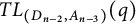 $TL_{(D_{n-2}, A_{n-3})}(q)$
where each coset diagram has an odd number of
$TL_{(D_{n-2}, A_{n-3})}(q)$
where each coset diagram has an odd number of
 $\wedge $
arrows (as discussed in Remark 5.3).
$\wedge $
arrows (as discussed in Remark 5.3).


This map is clearly a bijection, as starting from any oriented Temperley–Lieb diagram for the anti-spherical module in rank
 $n-2$
, we can insert the degree zero arc in the position corresponding to
$n-2$
, we can insert the degree zero arc in the position corresponding to ![]() to obtain an oriented Temperley–Lieb diagram for the anti-spherical module in rank n and these maps are clearly inverse to each other.
to obtain an oriented Temperley–Lieb diagram for the anti-spherical module in rank n and these maps are clearly inverse to each other.
Acknowledgements
We are thankful to Jon Brundan and Catharina Stroppel for interesting and informative conversations and to the MFO workshop “Character Theory and Categorification” for providing an excellent environment for collaboration. We are also very thankful to the anonymous referee for their incredibly detailed comments, which improved the exposition of the paper a great deal.


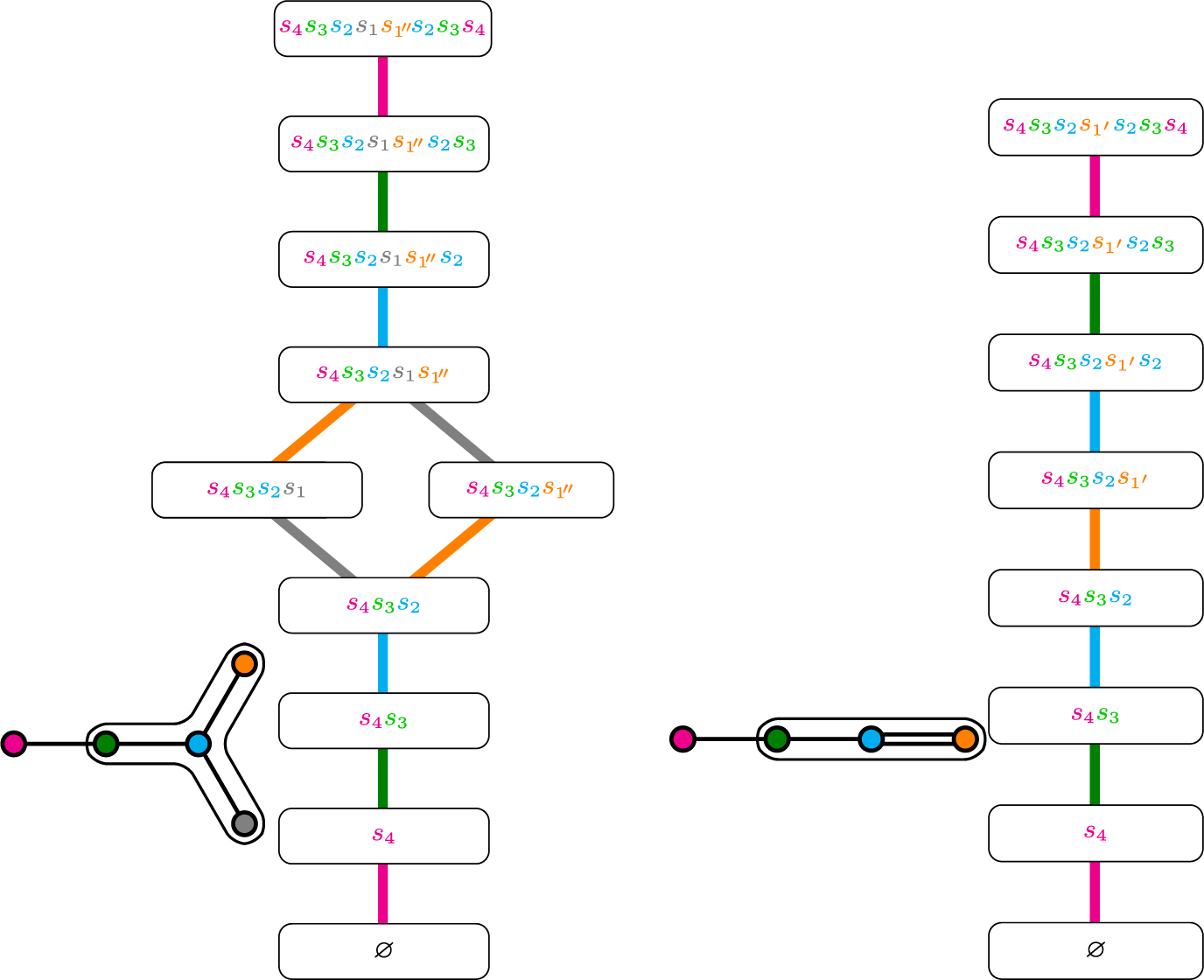


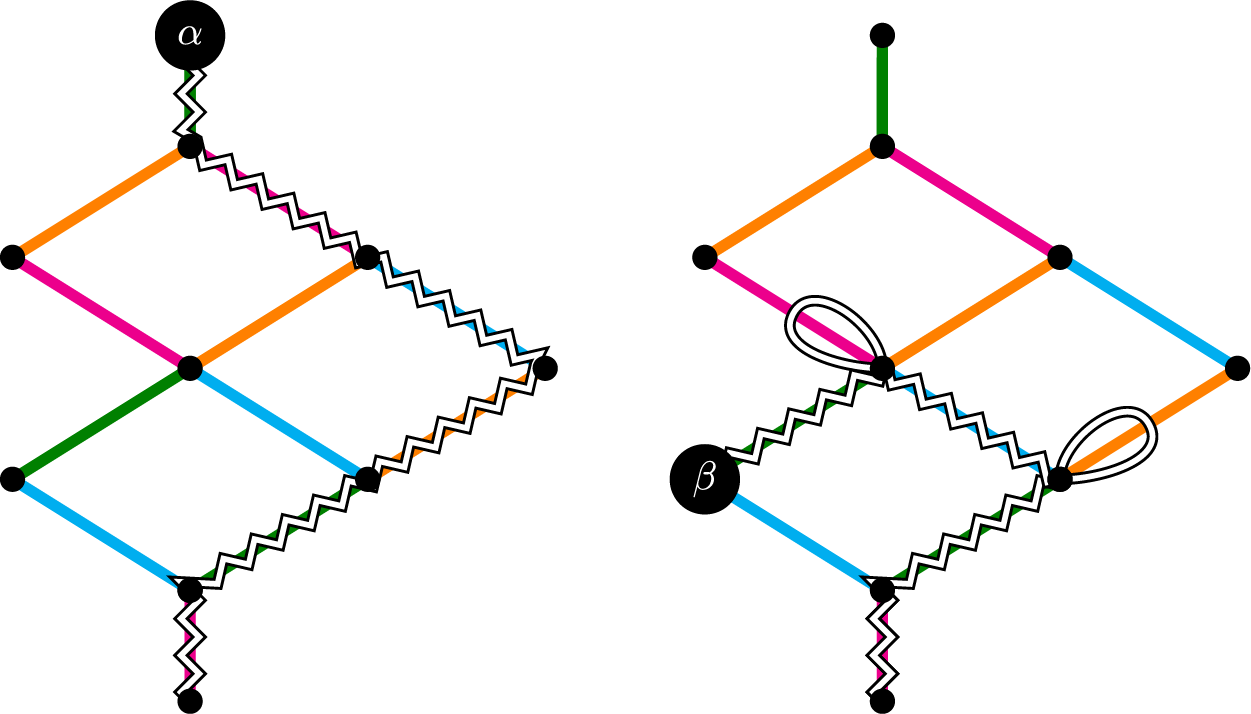


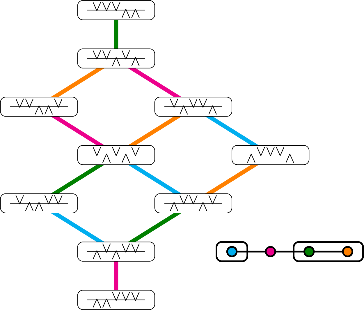


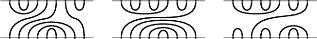


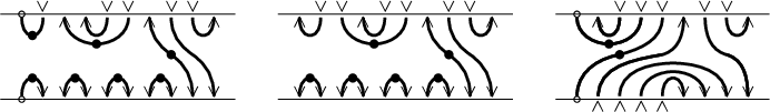


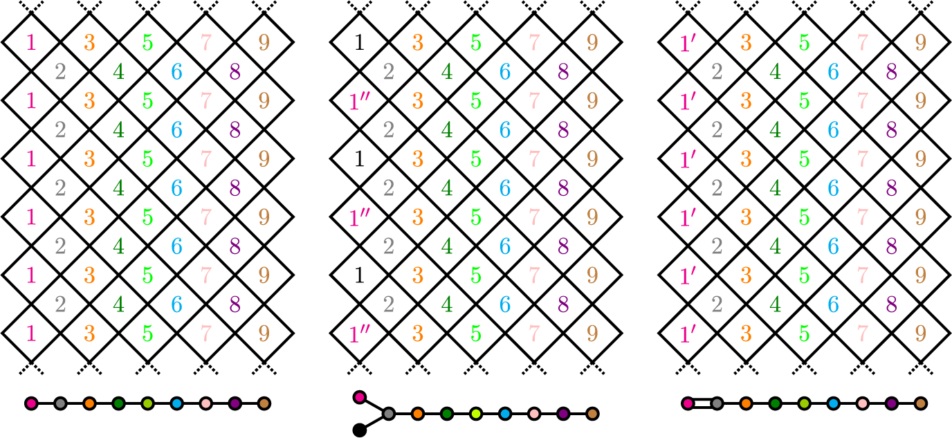


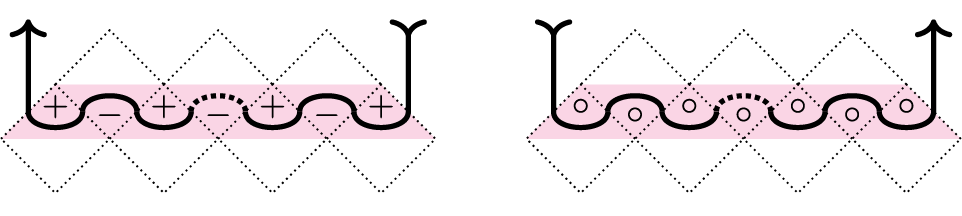
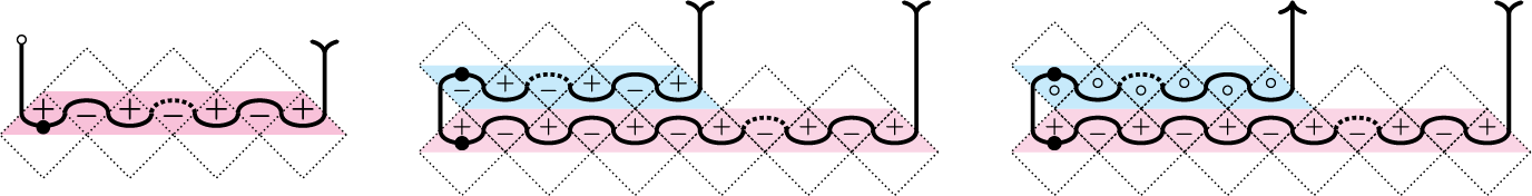
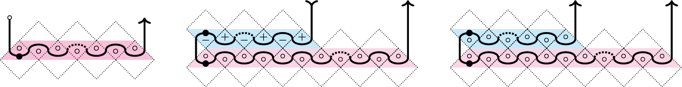
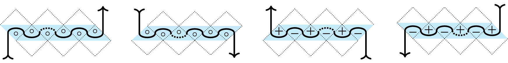


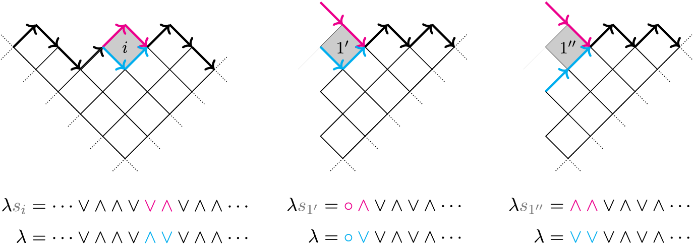


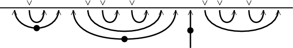


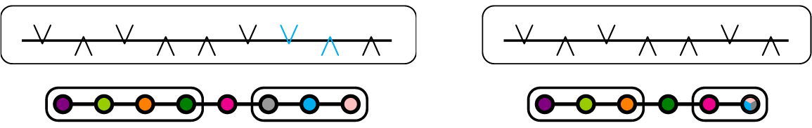

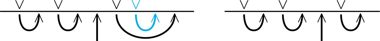


 Open access