


1 Introduction
The assumption of local independence (LI) postulates the unsystematic nature of any effect that differentiates the response behavior of individuals above and beyond the constructs assessed by a test. However, a variety of person-, test-, or context-related effects can cause local dependence (LD), which threatens model validity, invalidates the likelihood, and results in biased estimates of both item parameters and construct degrees (see, e.g., Andrich, Reference Andrich and Embretson1985; Chen & Thissen, Reference Chen and Thissen1997; Edwards et al., Reference Edwards, Houts and Cai2018; Junker, Reference Junker1991; Reese, Reference Reese1995; Tuerlinckx & De Boeck, Reference Tuerlinckx and De Boeck2001; Yen, Reference Yen1984; Yen, Reference Yen1993; Zenisky et al., Reference Zenisky, Hambleton and Sired2002). A well-known example is that of artificially inflated slopes of dependent items (see, e.g., Chen & Thissen, Reference Chen and Thissen1997; Edwards et al., Reference Edwards, Houts and Cai2018; Masters, Reference Masters1988), which manifests as positively biased discrimination parameters in item response theory (IRT) models and/or, equivalently, as positively biased loadings in factor analysis models.
The lack of a systematized perspective on the modeling of LD has however led to a fragmented literature with a plethora of indices, statistics, and approaches with different nomenclatures. As an example, Chen and Thissen (Reference Chen and Thissen1997) distinguished between surface LD (SLD), due to item similarity in content or location, and underlying LD (ULD), due to the existence of unmodeled constructs. Similar notions are known as “response dependence (RD)” and “trait dependence” (see, e.g., Marais & Andrich, Reference Marais and Andrich2008). However, while trait dependence is the same as ULD, RD differs from SLD as it models conditional item dependence. Similarly, Hoskens and De Boeck (Reference Hoskens and De Boeck1997) distinguished between “order dependency (OD)” and “combination dependency (CD)” where the former represents a factual (e.g., presentation order) or conceptual (e.g., mastering at different stages of learning) dependence, while the latter focuses on a whole set of items (e.g., gestalt-like effects or shared content). Although these conceptually resemble RD and SLD, they assume different modeling mechanisms.
This fragmentation is also a potential source of confusion. As stressed by Marais and Andrich (Reference Marais and Andrich2008), trait dependence and RD are “generally not distinguished clearly in the literature with the term multidimensionality used for trait dependence and the generic term local dependence used for both trait and response dependence”. Likewise, Edwards et al. (Reference Edwards, Houts and Cai2018) stressed that “there is substantial confusion surrounding the issues of dimensionality and local independence. Many researchers assume IRT models must be unidimensional to satisfy the local independence requirement,” a misbelief attributed to the misuse of early definitions of LI as operative definitions of uni-dimensionality (see, e.g., Hattie, Reference Hattie1985; Henning, Reference Henning1989). However, as one can imagine dependent items in a uni-dimensional context and independent items conditional to several traits, dimensionality is distinct from LI. Even so, while LD can be caused by multidimensionality, it can also occur in its absence if items directly affect each other.
Additional issues further complicate the topic: many available overall goodness-of-fit statistics are general purpose indices that neither are associated with specific sources of LD nor isolate LD from other model assumptions like dimensionality, monotonicity, or the specification of a latent trait density (see, e.g., Houts & Edwards, Reference Houts and Edwards2015; Liu & Maydeu-Olivares, Reference Liu and Maydeu-Olivares2012); multi-dimensional IRT models are empirically indistinguishable from locally dependent uni-dimensional IRT models (Ip, Reference Ip2010); different mechanisms can generate the same amount of LD: extremely high specific-to-general slope ratios for ULD models (based on a bifactor model) can mirror the polychoric correlations generated by models with mid-range to high SLD (Houts & Edwards, Reference Houts and Edwards2015), a result that might explain why some mechanisms like SLD are considered to be more easily detectable than others like ULD (see, e.g., Chen & Thissen, Reference Chen and Thissen1997; Houts & Edwards, Reference Houts and Edwards2013).
The present manuscript attempts a systematization and generalization of some approaches to LD based on a framework suggested by Noventa et al. (Reference Noventa, Heller and Kelava2024, Reference Noventa, Heller, Ye and Kelava2025) that, drawing on the abstract nature of knowledge space theory (KST; see, e.g., Falmagne & Doignon, Reference Falmagne and Doignon2011), unifiesFootnote 1 models from IRT, KST, and cognitive diagnostic assessment (CDA, see, e.g., Rupp et al., Reference Rupp, Templin and Henson2010; von Davier & Lee, Reference Davier and Lee2019). The gist of this framework is the observation that all these theories postulate some conditional relation between item responses and latent knowledge, attributes, skills, or traits. Consider the item “
$2+3=?$
 .” In the original KST approach, one wonders if the capability of mastering the item (the latent knowledge) will also allow to solve it (the observed response). In a CDA/competence-based KST approach, one wonders if an individual possesses the (dichotomous) skills/attributes (e.g., basic mental calculation skills) needed to master or solve the item. In an IRT approach, one wonders if an individual can master or solve the item given some continuous measure of the mental ability. Only two primitives are needed to formalize this state of affairs: the KST notion of “structure,” which formalizes the different entities in the theories, and the notion of “process,” which formalizes their relations. Intuitively, given a domain of elements of a given “sort” (e.g., items or attributes), a structure is the collection of all the combinations of these elements (called states) that can exist according to some existing hierarchy between the elements themselves. Consider the items “
$2+3=?$
.” In the original KST approach, one wonders if the capability of mastering the item (the latent knowledge) will also allow to solve it (the observed response). In a CDA/competence-based KST approach, one wonders if an individual possesses the (dichotomous) skills/attributes (e.g., basic mental calculation skills) needed to master or solve the item. In an IRT approach, one wonders if an individual can master or solve the item given some continuous measure of the mental ability. Only two primitives are needed to formalize this state of affairs: the KST notion of “structure,” which formalizes the different entities in the theories, and the notion of “process,” which formalizes their relations. Intuitively, given a domain of elements of a given “sort” (e.g., items or attributes), a structure is the collection of all the combinations of these elements (called states) that can exist according to some existing hierarchy between the elements themselves. Consider the items “
$2+3=?$
 ” and “
$\frac {1}{2}+\frac {1}{3}=?,$
” and “
$\frac {1}{2}+\frac {1}{3}=?,$
 ” if one assumes that an individual capable of mastering the latter must also be able to master the former (but not vice versa) the structure contains three states: a) no items mastered, b) only “
$2+3=?$
” if one assumes that an individual capable of mastering the latter must also be able to master the former (but not vice versa) the structure contains three states: a) no items mastered, b) only “
$2+3=?$
 ” mastered, and c) both items mastered. In other words, if a similar structure is imposed, the responses would form an incomplete pairwise contingency table in which a cell is missing by design. As a consequence, response patterns that are incompatible with the hierarchy (e.g., only “
$\frac {1}{2}+\frac {1}{3}=?$
” mastered, and c) both items mastered. In other words, if a similar structure is imposed, the responses would form an incomplete pairwise contingency table in which a cell is missing by design. As a consequence, response patterns that are incompatible with the hierarchy (e.g., only “
$\frac {1}{2}+\frac {1}{3}=?$
 ” is solved) must be modeled stochastically in order to obtain a complete contingency table for the responses. Structures made of items are called “knowledge structures” and model the latent knowledge (items mastered) and the response patterns (items solved). “Competence structures” are instead used to organize skills, attributes, and traits. The notion of process instead makes explicit the relation between the states of different structures. Following a nomenclature coined by Hutchinson (Reference Hutchinson1991), a process capturing the attempt of individuals to master an item based on their ability (i.e., connecting a competence structure to a knowledge structure) is called a p-process, while a process capturing the effects of pure chance on item solving (i.e., connecting two knowledge structures) is called a g-process. Assessment models are then obtained by connecting processes and by setting assumptions on their conditional probabilities. Two operations are common: “factorization,” which rewrites a probability as a product of different terms (e.g., assuming LI) and “reparameterization,” which provides alternative functional forms to the models (e.g., using a logit or a probit link function). Interestingly, a simple sequence of a p-process and a g-process provides a taxonomy of most KST, CDA, and IRT models. As an example, in a 3-parameter logistic (3PL) model, the p-process is the 2-parameter logistic (2PL) model, while the g-process either adds a constant guessing parameter or some ability-based guessing (San Martin et al., Reference San Martin, del Pino and De Boeck2006).
The same abstract approach used to construct a taxonomy of KST, CDA, and IRT models is here applied to systematize the different approaches to LD. As the focus of the present manuscript is to frame LD models from a unified perspective, a greater relevance is given to theoretical rather than applied aspects, since they allow to understand how LD models are systematized, related, and therefore built through the choice of specific assumptions, thus also suggesting new families of models. Moreover, it should be stressed that since the focus of the manuscript is to consider a unified perspective encompassing KST, IRT, and CDA models only categorical response variables and the associated probabilistic models are considered. The manuscript will not cover approaches like factor analysis of continuous response variables and associated important techniques like the study of residuals to model LD. Nonetheless, due to the well-established equivalence between two-parameter IRT models and factor analysis of dichotomous variables (see, e.g., Takane & de Leeuw, Reference Takane and de Leeuw1987), the results also hold for the latter.
As an immediate consequence of considering a top-down approach that moves from general abstract primitives, the existence of two main primitives of assessment models (i.e., structure and process) implies the existence of two distinct but not mutually exclusive mechanisms of modeling LD (i.e., via the structure or via the process). Modeling via the structure is of a deterministic nature, while modeling via the process is of a probabilistic nature. This has direct implications for the approaches used in modeling local LD: two major approaches here called “probabilistic” and “deterministic” LD can be identified. In probabilistic LD, which encompasses most IRT approaches to LD, a power set structure is considered and models with only a p-process are applied. This approach captures situations in which items do not directly affect each other (a power set corresponds to a complete contingency table and therefore allows for all possible response patterns). As in such cases, LD is modeled only by assuming a specific functional form of the p-process, LD alters the likelihood of improbable but possible patterns and it is of a purely stochastic nature. On the converse, in deterministic LD, which encompasses some IRT approaches and the KST-IRT models introduced by Noventa et al. (Reference Noventa, Spoto, Heller and Kelava2019), a structure prohibits certain response patterns by imposing direct effects between the items (i.e., by imposing with a structure an incomplete contingency table of responses). In such a case, the only way to recover those response patterns that are in principle prohibited is to impose a g-process over the deterministic structure. The distinction between probabilistic and deterministic LD should therefore not be conceived as a distinction between probabilistic and non-probabilistic models, but as an indication on whether a deterministic constraint is imposed or not (i.e., the structure) prior to the stochastic modeling of the response patterns (i.e., the processes). A Guttman scalogram of the items “
$2+3=?$
 ” and “
$\frac {1}{2}+\frac {1}{3}=?$
” and “
$\frac {1}{2}+\frac {1}{3}=?$
 ” illustrates the differences. The IRT approach to Guttman’s scaling is to fit a Rasch model (p-process) under the assumption of LI (which requires a power set, i.e., all possible states). Instead, within a KST-IRT perspective, Guttman’s scaling is captured by a p-process between a competence structure (e.g., skills, attributes, or traits) and a knowledge structure with three states as described above, which is known as a “chain.” A g-process then leads to all four possible response patterns.
We argue that such a distinction has four main advantages: First, it allows for the modeling of different phenomena within psychological and educational testing that require distinct substantive assumptions. A probabilistic LD approach may be applied in clinical assessment, since many psychological disorders (e.g., major depressive episode) are diagnosed when a certain number of independent criteria are met (e.g., having suicidal thoughts and lack of appetite). Conversely, performance-based assessments (e.g., intelligence or learning disorders tests) are well-suited for a deterministic LD perspective since items are usually administered according to a difficulty order, and specific response patterns are expected. Of course, instances where applying a deterministic LD approach within clinical assessment would be preferable, and vice versa, might manifest (e.g., one might argue that feeling sadness might precede having suicidal thoughts). Second, it might explain why some forms of LD are more easily detected. While probabilistic LD and multi-dimensionality are both modeled within the p-process, deterministic LD is modeled by a separate mechanism. As most IRT approaches to LD appear to be of a probabilistic form, with the exception of SLD and boundary copula functions that are examples of deterministic LD, this might explain why extreme ULD is needed to mirror mid-range to high SLD (Houts & Edwards, Reference Houts and Edwards2015). Third, as deterministic LD can model situations that are too extreme for probabilistic LD, it allows to avoid extreme values of the model parameters (e.g., inflated slopes). Fourth, while some LD sources might be modeled as either deterministic or probabilistic depending on their magnitude and on the substantive nature of the items (e.g., Guttman’s scaling), other sources might be of only a probabilistic or a deterministic nature (e.g., the categories of a polytomous item). Models capturing a polytomous item and models representing multiple dependent dichotomous items appear indeed to be formally equivalent up to the interpretation of the elements of the structure. As a consequence, structures provide a natural approach to testlets, which are often analyzed by summing LD binary items and scoring them as a single polytomous item.
As to the plan of the work. In Section 2, we provide basic notions about LD and introduce the unified framework. In Section 3, probabilistic and deterministic LD are systematized. As the purpose of this work is to frame some approaches to LD, these are not introduced but directly derived. The appendices of the manuscript cover more in detail some technical or ancillary aspects: Appendix A highlights the relation between SLD and the approach of Ackerman and Spray (Reference Ackerman and Spray1987), Appendix B provides the generalization of the results of Huynh (Reference Huynh1994, Reference Huynh1996) to probabilistic and deterministic LD, while Appendix C provides some considerations on the so-called “disordered-threshold controversy.” Finally, the Supplementary Material to the manuscript also provides a brief list of indices, statistics, and approaches to LD.
2 Preliminary notions
In this section, we firstly recall the notions of strong and weak LI and discuss the pairwise contingency tables associated with LD. Secondly, we introduce the primitives of the unified framework.
2.1 Basic notions of LD: Strong and weak LI and contingency tables
Let Q be a set of dichotomous items
$q_i\in Q$
 for
$i\in \{1,\dots , |Q|\}$
for
$i\in \{1,\dots , |Q|\}$
 , and let
$X_i$
, and let
$X_i$
 be the random variable with realizations
$x_i\in \{0,1\}$
be the random variable with realizations
$x_i\in \{0,1\}$
 , expressing if the answer to the item
$q_i\in Q$
, expressing if the answer to the item
$q_i\in Q$
 is correct or incorrect. LI is often formalized as probabilistic independence of the random variables
$X_i$
is correct or incorrect. LI is often formalized as probabilistic independence of the random variables
$X_i$
 conditional to some latent variable
$\theta \in \mathbb {R}$
conditional to some latent variable
$\theta \in \mathbb {R}$
 capturing the construct. A common parametric definition is the strong form

where the joint probability of the random vector
$X = \{X_1,\ldots ,X_n\}$
 with realizations
$x\in \{0,1\}^{|Q|}$
with realizations
$x\in \{0,1\}^{|Q|}$
 is expressed as the product of the marginal probabilities of the random variables
$X_i$
is expressed as the product of the marginal probabilities of the random variables
$X_i$
 .
$\Gamma $
.
$\Gamma $
 comprises the collections
$\Gamma _i$
comprises the collections
$\Gamma _i$
 of parameters of the item response function (IRF) for the item
$q_i\in Q$
of parameters of the item response function (IRF) for the item
$q_i\in Q$
 . In principle, IRFs might be parametric or non-parametric. The 4-parameter logistic model (4PL) is given by

where
$\Gamma _i=\{a_i, b_i, c_i, d_i\}$
 contains the discrimination, difficulty, guessing, and slipping parameters. The 3PL model is obtained for
$d_i=0$
contains the discrimination, difficulty, guessing, and slipping parameters. The 3PL model is obtained for
$d_i=0$
 , the 2PL/Birnbaum model for
$d_i=c_i =0$
, the 2PL/Birnbaum model for
$d_i=c_i =0$
 , the 1PL/Rasch model by also setting
$a_i=1$
, the 1PL/Rasch model by also setting
$a_i=1$
 . If the parameter
$c_i$
. If the parameter
$c_i$
 is replaced by the function
$c_i(\theta )=(1+\exp {(\tilde {c}_i-\theta )})^{-1}$
is replaced by the function
$c_i(\theta )=(1+\exp {(\tilde {c}_i-\theta )})^{-1}$
 for some
$\tilde {c}_i\in \mathbb {R,}$
for some
$\tilde {c}_i\in \mathbb {R,}$
 the model is known as 1PL ability-based guessing (1PLAG; Martin et al., Reference San Martin, del Pino and De Boeck2006). The same principle can be applied to the slipping parameter by considering
$d_i(\theta )=(1+\exp {(\theta - \tilde {d}_i)})^{-1}$
the model is known as 1PL ability-based guessing (1PLAG; Martin et al., Reference San Martin, del Pino and De Boeck2006). The same principle can be applied to the slipping parameter by considering
$d_i(\theta )=(1+\exp {(\theta - \tilde {d}_i)})^{-1}$
 .
.
In spite of its simplicity, LI (1) is extremely restrictive and in practical applications is often replaced by a null conditional item covariance form, known as pairwise or weak LI (see, e.g., Stout, Reference Stout2002), given by

In principle, for both LI (1) and (3), one can consider a likelihood of the form
$P(X|\Gamma ,\Theta )$
 in which
$\Theta \in \mathbb {R}^d$
in which
$\Theta \in \mathbb {R}^d$
 and d is the number of latent dimensions. The smallest value of d such that LI is satisfied provides a traditional definition of test dimensionality, which has the strong limitation of assuming that all dimensions have the same relevance (see, e.g., McDonald, Reference McDonald1981; Stout, Reference Stout1990). For the present work, however, any unaccounted trait, irrespective of its major or minor nature, implies a violation of LI (1) or (3).
Weak LI (3) constitutes the backbone of many procedures and indices to detect violations of LI. Excess covariation or association in the pairwise marginal contingency tables of items
$q_i,q_{i'}$
 is detected by comparing the observed proportions
$p_{x_i x_{i'}}$
is detected by comparing the observed proportions
$p_{x_i x_{i'}}$
 with the expected ones
$p^{*}_{x_i x_{i'}}$
with the expected ones
$p^{*}_{x_i x_{i'}}$
 for a chosen IRT model, that is,

where
$f(\theta )$
 is the probability density function of the ability. For the present work, we identify two relevant patterns of LD that manifest themselves as pairwise incomplete contingency tables, that is,

where Table A corresponds to a prerequisite relation between items so that one cannot master item
$q_{i'}$
 if item
$q_i$
if item
$q_i$
 is not mastered (e.g., if a person masters the item “
$\frac {1}{2}+\frac {1}{3} = ?,$
is not mastered (e.g., if a person masters the item “
$\frac {1}{2}+\frac {1}{3} = ?,$
 ” then it also masters the item “
$2+3=?$
” then it also masters the item “
$2+3=?$
 ,” but not vice versa), while Table B captures two items that are either mastered or failed jointly (e.g., if a person masters the item “
$2+3=?$
,” but not vice versa), while Table B captures two items that are either mastered or failed jointly (e.g., if a person masters the item “
$2+3=?$
 ,” it also masters the item “
$3+2 = ?$
,” it also masters the item “
$3+2 = ?$
 ,” and vice versa). The fact that items manifesting dependence show artificially inflated slopes under LI is apparent for a 2PL model (we set
$c_i=d_i=0$
,” and vice versa). The fact that items manifesting dependence show artificially inflated slopes under LI is apparent for a 2PL model (we set
$c_i=d_i=0$
 for what follows), for which both Tables A and B are obtained in the limit
$a_i, a_{i'}\rightarrow \infty $
for what follows), for which both Tables A and B are obtained in the limit
$a_i, a_{i'}\rightarrow \infty $
 . If
$b_{i'}> b_i$
. If
$b_{i'}> b_i$
 , one obtains Table A since individuals with
$\theta> b_{i'}$
, one obtains Table A since individuals with
$\theta> b_{i'}$
 ,
$b_{i'}> \theta > b_i$
,
$b_{i'}> \theta > b_i$
 , and
$\theta < b_{i}$
, and
$\theta < b_{i}$
 , respectively, belong to
$p_{11}$
, respectively, belong to
$p_{11}$
 ,
$p_{10}$
,
$p_{10}$
 , and
$p_{00}$
, and
$p_{00}$
 . Exception is given by individuals with
$\theta =b_i$
. Exception is given by individuals with
$\theta =b_i$
 (
$\theta = b_{i'}$
(
$\theta = b_{i'}$
 ), which belong to both
$p_{00}$
), which belong to both
$p_{00}$
 and
$p_{10}$
and
$p_{10}$
 (
$p_{10}$
(
$p_{10}$
 and
$p_{11}$
and
$p_{11}$
 ). Similarly, if
$b_i=b_{i'}$
). Similarly, if
$b_i=b_{i'}$
 , then one approximates Table B since individuals with
$\theta> b_{i}$
, then one approximates Table B since individuals with
$\theta> b_{i}$
 (
$\theta < b_{i}$
(
$\theta < b_{i}$
 ) belong to
$p_{11}$
) belong to
$p_{11}$
 (
$p_{00}$
(
$p_{00}$
 ), while individuals with
$\theta =b_i$
), while individuals with
$\theta =b_i$
 are distributed among all cells. These behaviors are apparent in the following LI Tables (only the values of the 2PL’s item parameters are reported in parentheses as
$c_i=d_i=0$
are distributed among all cells. These behaviors are apparent in the following LI Tables (only the values of the 2PL’s item parameters are reported in parentheses as
$c_i=d_i=0$
 is set for both items). The density
$f(\theta )$
is set for both items). The density
$f(\theta )$
 is a standard normal. Starting from Table LI-1 and moving to the right, the value of
$b_2$
is a standard normal. Starting from Table LI-1 and moving to the right, the value of
$b_2$
 increases, and the tables approximate Table A. Moving from top to bottom, the discrimination parameters
$a_i$
increases, and the tables approximate Table A. Moving from top to bottom, the discrimination parameters
$a_i$
 increase, and Tables LI-4 and LI-5 approximate Tables B and A. However, under LI,
$p_{11}$
increase, and Tables LI-4 and LI-5 approximate Tables B and A. However, under LI,
$p_{11}$
 also approaches zero as in Table LI-6.


2.2 Unified framework: Taxonomy of CDA, KST, and IRT models
Before formally introducing the primitives of the framework (structure and process) and the main operations (factorization and reparameterization), let us reformulate the 4PL model of Eq. (2) to provide an intuitive understanding of these notions. A little algebra allows to rewrite the 4PL model as


where
$\pi (K_i=1|a_i,b_i,\theta )$
 is the IRF of a 2-parameter model in which the random variable
$K_i$
is the IRF of a 2-parameter model in which the random variable
$K_i$
 represents if the i-th item is mastered or not. According to Eq. (6), an item can be solved (
$X_i=1$
represents if the i-th item is mastered or not. According to Eq. (6), an item can be solved (
$X_i=1$
 ) either from guessing a non-mastered item (
$K_i=0$
) either from guessing a non-mastered item (
$K_i=0$
 ) or from not slipping on a mastered item (
$K_i = 1$
) or from not slipping on a mastered item (
$K_i = 1$
 ). By definition, it holds that
$c_i := P(X_i=1|K_i=0)$
). By definition, it holds that
$c_i := P(X_i=1|K_i=0)$
 and
$d_i := P(X_i=0|K_i=1)$
and
$d_i := P(X_i=0|K_i=1)$
 . The conditional probabilities
$P(X_i|K_i)$
. The conditional probabilities
$P(X_i|K_i)$
 and
$\pi (K_i|\theta ),$
and
$\pi (K_i|\theta ),$
 respectively, characterize the g-process and the p-process. The former captures the relation between the knowledge of the item (
$K_i$
respectively, characterize the g-process and the p-process. The former captures the relation between the knowledge of the item (
$K_i$
 ) and the actual response (
$X_i$
) and the actual response (
$X_i$
 ), and provides the so-called left-side added parameters (Thissen & Steinberg, Reference Thissen and Steinberg1986), while the latter captures the relation between the latent trait (
$\theta $
), and provides the so-called left-side added parameters (Thissen & Steinberg, Reference Thissen and Steinberg1986), while the latter captures the relation between the latent trait (
$\theta $
 ) and the knowledge of the item (
$K_i$
) and the knowledge of the item (
$K_i$
 ), and corresponds to the 2-parameter IRF. Eq. (7) is an example of reparameterization by means of a logit link function endowing the 2-parameter model with a specific form. In a traditional latent variable approach, the random variable
$K_i$
), and corresponds to the 2-parameter IRF. Eq. (7) is an example of reparameterization by means of a logit link function endowing the 2-parameter model with a specific form. In a traditional latent variable approach, the random variable
$K_i$
 (
$X_i$
(
$X_i$
 ) represents the latent classes associated with mastering (solving) and not mastering (not solving). A feature of the unified framework is to model the structure of these latent classes. Indeed, although
$X_i$
) represents the latent classes associated with mastering (solving) and not mastering (not solving). A feature of the unified framework is to model the structure of these latent classes. Indeed, although
$X_i$
 and
$K_i$
and
$K_i$
 are different random variables, they are both defined over the same states (i.e., the same structure): an empty state (no item) and a state containing only one item. More in general, latent classes associated with items, responses, attributes, and traits are captured via the notion of structure: let D be a non-empty domain of elements
$d_i\in D$
are different random variables, they are both defined over the same states (i.e., the same structure): an empty state (no item) and a state containing only one item. More in general, latent classes associated with items, responses, attributes, and traits are captured via the notion of structure: let D be a non-empty domain of elements
$d_i\in D$
 . Any pair like
$(D,\mathcal {Y}),$
. Any pair like
$(D,\mathcal {Y}),$
 where
$\mathcal {Y}$
where
$\mathcal {Y}$
 is a family of subsets
$Y\subseteq D$
is a family of subsets
$Y\subseteq D$
 such that
$\{\emptyset , D\}\subseteq \mathcal {Y}\subseteq 2^D$
such that
$\{\emptyset , D\}\subseteq \mathcal {Y}\subseteq 2^D$
 is called a structure, and any subset like
$Y\in \mathcal {Y}$
is called a structure, and any subset like
$Y\in \mathcal {Y}$
 a state. Informally, the domain is omitted. Figure 1 provides examples of structures on
$D=\{d_1, d_2,d_3\}$
a state. Informally, the domain is omitted. Figure 1 provides examples of structures on
$D=\{d_1, d_2,d_3\}$
 .
.
Examples of structures on
$D=\{d_1, d_2, d_3\}$
 .
.

Figure 1 Long description
The figure consists of three panels.
Panel 1, on the left, shows a linear graph with four nodes connected by a single horizontal line. From left to right, the nodes are labeled with the empty set symbol, the set containing d sub 1, the set containing d sub 1 and d sub 2, and finally D. Below this is the equation Y sub 1 equals the set containing the empty set, the set of d sub 1, the set of d sub 1 and d sub 2, and D.
Panel 2, in the center, shows a hexagonal graph structure. It starts at a leftmost node labeled with the empty set symbol, which branches into two paths. The top path goes to a node labeled with the set of d sub 1, then to the set of d sub 1 and d sub 2. The bottom path goes to a node labeled with the set of d sub 3, then to the set of d sub 1 and d sub 3. A diagonal line connects the set of d sub 1 to the set of d sub 1 and d sub 3. Both paths converge at a rightmost node labeled D. Below is the equation Y sub 2 equals the set containing the empty set, the set of d sub 1, the set of d sub 3, the set of d sub 1 and d sub 3, the set of d sub 1 and d sub 2, and D.
Panel 3, on the right, shows a more complex graph resembling a projection of a three-dimensional cube. It starts at the empty set symbol on the left and branches into three paths. The nodes are labeled with various combinations of d sub 1, d sub 2, and d sub 3, including the set of d sub 1, the set of d sub 2, the set of d sub 3, the set of d sub 1 and d sub 2, the set of d sub 1 and d sub 3, and the set of d sub 2 and d sub 3. All paths converge at the rightmost node D. Below is the equation Y sub 3 equals 2 super D.
A structure like
$\mathcal {Y}_1$
 , in which the elements form a linearly ordered set, is called a chain, a structure like
$\mathcal {Y}_3$
, in which the elements form a linearly ordered set, is called a chain, a structure like
$\mathcal {Y}_3$
 is a power set
$2^D$
is a power set
$2^D$
 , while
$\mathcal {Y}_2$
, while
$\mathcal {Y}_2$
 is an arbitrary relation. In all these structures, the states are latent classes ordered by set inclusion. Nominal latent classes are instead represented by a collection of singletons of mutually exclusive elements. As an example,
$\mathcal {Y}=\{\{d_1\},\{d_2\}\}$
is an arbitrary relation. In all these structures, the states are latent classes ordered by set inclusion. Nominal latent classes are instead represented by a collection of singletons of mutually exclusive elements. As an example,
$\mathcal {Y}=\{\{d_1\},\{d_2\}\}$
 represents the collection of the latent classes of the mutually exclusive elements
$d_1$
represents the collection of the latent classes of the mutually exclusive elements
$d_1$
 and
$d_2$
and
$d_2$
 (e.g., males and females). If a probability distribution
$P_{\mathcal {Y}}: \mathcal {Y}\rightarrow [0,1]$
(e.g., males and females). If a probability distribution
$P_{\mathcal {Y}}: \mathcal {Y}\rightarrow [0,1]$
 is defined so that
$P(Y)$
is defined so that
$P(Y)$
 is the probability of the state
$Y\in \mathcal {Y}$
is the probability of the state
$Y\in \mathcal {Y}$
 (the subscript in
$P_{\mathcal {Y}}$
(the subscript in
$P_{\mathcal {Y}}$
 is omitted), the triple
$(D,\mathcal {Y}, P_{\mathcal {Y}})$
is omitted), the triple
$(D,\mathcal {Y}, P_{\mathcal {Y}})$
 is called a probabilistic structure, and provides a set-theoretical recast of a contingency table for cross-classified dichotomous variables. Every state
$Y\in \mathcal {Y}$
is called a probabilistic structure, and provides a set-theoretical recast of a contingency table for cross-classified dichotomous variables. Every state
$Y\in \mathcal {Y}$
 (e.g.,
$Y=\{d_1,d_3\}$
(e.g.,
$Y=\{d_1,d_3\}$
 ) labels a non-empty cell of the table since it can be mapped into the realization
$y\in \{0,1\}^{|D|}$
) labels a non-empty cell of the table since it can be mapped into the realization
$y\in \{0,1\}^{|D|}$
 (e.g.,
$y=(1,0,1)$
(e.g.,
$y=(1,0,1)$
 ), of a random vector Y such that
$Y_i = 1$
), of a random vector Y such that
$Y_i = 1$
 iff
$d_i\in Y$
iff
$d_i\in Y$
 . The state probability
$P(Y)$
. The state probability
$P(Y)$
 captures the associated probability/frequency. If
$\mathcal {Y}=2^D$
captures the associated probability/frequency. If
$\mathcal {Y}=2^D$
 , the table is complete. If
$\mathcal {Y}\subset 2^D$
, the table is complete. If
$\mathcal {Y}\subset 2^D$
 , the table is incomplete with structural zeros (missing cells by design) corresponding to the subsets in
$2^D\setminus \mathcal {Y}$
, the table is incomplete with structural zeros (missing cells by design) corresponding to the subsets in
$2^D\setminus \mathcal {Y}$
 .
.
Table summarizing the taxonomy of families of KST-CDA-IRT models based on the application of p- and g-processes

Table 1 Long description
The table is organized into three columns: Family, p-process, and g-process.
* Family 1: p-process is Not applied; g-process is Not applied. Models include K S T and C D A.
* Family 2: p-process is Applied; g-process is Not applied. Models include P K S T, P C D A, and D I N A.
* Family 3: p-process is Not applied; g-process is Applied. Models include G K S T, G C D A, and D I N O.
* Family 4: p-process is Applied; g-process is Applied. Models include P G K S T, P G C D A, and G D I N A.
Structures can then be given different interpretations, we provide here some examples:
-
• Given a domain Q of dichotomous items $q_i$
 , a (probabilistic) knowledge structure is a triple
$(Q,\mathcal {K}, \pi )$
with
$\mathcal {K}$
a family of knowledge states
$K\subseteq Q$
and
$\pi : \mathcal {K}\rightarrow [0,1]$
a probability distribution. As an example, let
$Q=\{q_1,q_2\}$
, then a chain of the form
$\mathcal {K}_A=\{\emptyset , \{q_1\}, \{q_1, q_2\}\}$
as in Table A represents a sequence of items such that
$q_2$
cannot be mastered unless
$q_1$
is mastered (e.g., “
$2+3=?$
” and “
$\frac {1}{2}+\frac {1}{3}=?$
” ). A power set
$2^Q =\{\emptyset , \{q_1\}, \{q_2\}, \{q_1, q_2\}\} $
would capture the independence of two items (e.g., “Having suicidal thoughts” and “Lacking appetite”). The power set will be shown to be necessary for LI. A structure like
$\mathcal {K}_B=\{\emptyset ,\{q_1, q_2\}\}$
as in Table B is well-suited if items are always mastered or failed jointly (e.g., “
$2+3=?$
” and “
$3+2=?$
”). Items like these are known in KST as “equally informative items.”
, a (probabilistic) knowledge structure is a triple
$(Q,\mathcal {K}, \pi )$
with
$\mathcal {K}$
a family of knowledge states
$K\subseteq Q$
and
$\pi : \mathcal {K}\rightarrow [0,1]$
a probability distribution. As an example, let
$Q=\{q_1,q_2\}$
, then a chain of the form
$\mathcal {K}_A=\{\emptyset , \{q_1\}, \{q_1, q_2\}\}$
as in Table A represents a sequence of items such that
$q_2$
cannot be mastered unless
$q_1$
is mastered (e.g., “
$2+3=?$
” and “
$\frac {1}{2}+\frac {1}{3}=?$
” ). A power set
$2^Q =\{\emptyset , \{q_1\}, \{q_2\}, \{q_1, q_2\}\} $
would capture the independence of two items (e.g., “Having suicidal thoughts” and “Lacking appetite”). The power set will be shown to be necessary for LI. A structure like
$\mathcal {K}_B=\{\emptyset ,\{q_1, q_2\}\}$
as in Table B is well-suited if items are always mastered or failed jointly (e.g., “
$2+3=?$
” and “
$3+2=?$
”). Items like these are known in KST as “equally informative items.” -
• Given a domain S of dichotomous attributes $s_a$
, a (probabilistic) competence structure is a triple
$(S,\mathcal {C}, \nu )$
with
$\mathcal {C}$
a family of competence states
$C\subseteq S$
and
$\nu : \mathcal {C}\rightarrow [0,1]$
a probability distribution. As an example, let
$S=\{s_1,s_2\},$
where
$s_1$
and
$s_2$
are, respectively, the attributes “addition” and “fraction” needed to master items ‘
$2+3=?$
’ and ‘
$\frac {1}{2}+\frac {1}{3}=?$
’. Assuming a power set
$2^S = \{\emptyset , \{s_1\}, \{s_2\}, \{s_1, s_2\}\}\}$
or a chain
$\mathcal {C}=\{\emptyset , \{s_1\}, \{s_1, s_2\}\}$
would imply different claims about the relation between these attributes. -
• Interpretations of structures are not limited to items and attributes. If the elements $d_i\in D$
are suitably interpreted so that the state
$\emptyset $
(D) represents the first (last) category, a chain like
$\mathcal {Y}_1$
can be used to model a Likert item or a polytomous attribute with four categories. As in IRT, one changes category by exceeding a “threshold,” we call item (attribute) thresholds the elements used to model a polytomous (attribute) item. For simplicity’s sake, we retain for these latter the same formalism of knowledge (competence) structures. We can then reinterpret a chain
$\mathcal {K}=\{\emptyset , \{q_1\}, \{q_1, q_2\}\}$
as a Likert item, and a chain
$\mathcal {C}=\{\emptyset , \{s_1\}, \{s_1, s_2\}\}$
as a polytomous attribute. Moreover, we can use the latter to define latent traits. Intuitively, one needs to generalize a finite chain like
$\mathcal {C}$
first to an infinite and then to an uncountable number of states (see Part III of Noventa et al., Reference Noventa, Ye, Kelava and Spoto2024, for details). If the elements
$s_a\in \mathcal {C}$
are interpreted as attribute thresholds, the resulting competence structure is an uncountable attribute
$\mathcal {C}$
capturing a continuum of competence states. This allows to link IRT to the other theories: like the random variables
$K_i$
and
$X_i$
were defined over the states of a finite structure, one can define a latent trait as a random variable
$\theta : \mathcal {C}\rightarrow \mathbb {R}$
defined over a continuous competence structure
$\mathcal {C}$
.


Given now two probabilistic structures
$(D,\mathcal {Y}, P_{\mathcal {Y}})$
 and
$(R,\mathcal {X}, P_{\mathcal {X}})$
and
$(R,\mathcal {X}, P_{\mathcal {X}})$
 , we can formalize the notion of process as a pair
$(\mathcal {Y}, \mathcal {X})$
, we can formalize the notion of process as a pair
$(\mathcal {Y}, \mathcal {X})$
 such that the probability distributions
$P_{\mathcal {Y}}$
such that the probability distributions
$P_{\mathcal {Y}}$
 and
$P_{\mathcal {X}}$
and
$P_{\mathcal {X}}$
 are related by


for all
$X\in \mathcal {X}$
 . Eq. (8) generalizes latent class models to the relation between two structures. Eq. (9) generalizes latent trait models in presence of an uncountable structure
$(D,\mathcal {Y}, P_{\mathcal {Y}})$
. Eq. (8) generalizes latent class models to the relation between two structures. Eq. (9) generalizes latent trait models in presence of an uncountable structure
$(D,\mathcal {Y}, P_{\mathcal {Y}})$
 that allows to replace the summation in Eq. (8) with an integral, and to substitute the integral of
$P(X|Y)$
that allows to replace the summation in Eq. (8) with an integral, and to substitute the integral of
$P(X|Y)$
 w.r.t. the probability measure
$P_{\mathcal {Y}}$
w.r.t. the probability measure
$P_{\mathcal {Y}}$
 with the integration w.r.t. a random variable
$\theta : \mathcal {Y}\rightarrow \mathbb {R}$
with the integration w.r.t. a random variable
$\theta : \mathcal {Y}\rightarrow \mathbb {R}$
 , with density function
$f(\theta )$
, with density function
$f(\theta )$
 . Using Eqs. (8) and (9), the taxonomy of assessment models represented in Table 1 is obtained by systematizing the processes involved in a model: we consider whether a p-process is absent or present and whether a g-process is absent, competence-independent, or competence-dependent. Since a power set structure
$(Q, 2^Q, P)$
. Using Eqs. (8) and (9), the taxonomy of assessment models represented in Table 1 is obtained by systematizing the processes involved in a model: we consider whether a p-process is absent or present and whether a g-process is absent, competence-independent, or competence-dependent. Since a power set structure
$(Q, 2^Q, P)$
 models the responses, the random vector X with realizations
$x\in \{0,1\}^{|Q|}$
models the responses, the random vector X with realizations
$x\in \{0,1\}^{|Q|}$
 is used in place of the state
$K\in 2^Q$
is used in place of the state
$K\in 2^Q$
 so that
$X_i=1$
so that
$X_i=1$
 if
$q_i\in K$
if
$q_i\in K$
 , zero otherwise. The p-processes
$\pi (K|C)$
, zero otherwise. The p-processes
$\pi (K|C)$
 and
$\pi (K|\theta )$
and
$\pi (K|\theta )$
 are referred to as state response functions (SRFs) as they generalize the IRFs to a set of items. Families of models in Table 1 therefore grow in generality from top to bottom and from left to right.
Most importantly, the general KST-IRT Eq. (14) is the marginalization of

which is a latent trait-extended version of Eq. (12) and allows to derive left side-added IRT models. As an example, a 4-parameter model follows from Eq. (19) by considering the structure
$\mathcal {K}=\{\emptyset , \{q_i\}\}$
 , that is,

where in the last passages, we have replaced the states
$\emptyset $
 and
$\{q_i\}$
and
$\{q_i\}$
 with the realizations of the random variable
$K_i$
with the realizations of the random variable
$K_i$
 and used the definitions
$c_i := P(X_i = 1|K_i = 0)$
and used the definitions
$c_i := P(X_i = 1|K_i = 0)$
 and
$d_i := P(X_i = 0|K_i = 1) $
and
$d_i := P(X_i = 0|K_i = 1) $
 . Application of a competence-based g-process yields models like the 1PLAG (Martin et al., Reference San Martin, del Pino and De Boeck2006).
Specific KST, CDA, and IRT models are derived from the models in Table 1 by imposing further assumptions on the p- and g-processes. Two common assumptions are associated with two operations: factorization rewrites a given probability as a product of terms and reparameterization gives new functional forms to the conditional probabilities by means of link functions as in generalized latent variable models.
As to factorization, an example is provided by LI (1). Applications of LI are common: in CDA and IRT, LI is used to factorize the conditional probabilities of Eqs. (10) and (11) into
$P(X|C)=\prod _{i=1}^{|Q|}P(X_i|C)$
 and
$P(X|\theta )=\prod _{i=1}^{|Q|}P(X_i|\theta )$
and
$P(X|\theta )=\prod _{i=1}^{|Q|}P(X_i|\theta )$
 . Similarly, imposing LI on the g-process
$P(X|K)$
. Similarly, imposing LI on the g-process
$P(X|K)$
 yields:

where
$K_i=1$
 if
$q_i\in K$
if
$q_i\in K$
 , zero otherwise. Eq. (20) in conjunction with Eq. (12) is known as the basic LI model (BLIM, see, e.g., Falmagne & Doignon, Reference Falmagne and Doignon2011). The parameters
$\eta _i$
, zero otherwise. Eq. (20) in conjunction with Eq. (12) is known as the basic LI model (BLIM, see, e.g., Falmagne & Doignon, Reference Falmagne and Doignon2011). The parameters
$\eta _i$
 and
$\beta _i$
and
$\beta _i$
 are known as lucky guess and careless error and are equivalent to the IRT guessing and slipping parameters
$c_i$
are known as lucky guess and careless error and are equivalent to the IRT guessing and slipping parameters
$c_i$
 and
$d_i$
and
$d_i$
 under LI (see below). The latent trait-extended version of the BLIM, known as
$\Theta $
under LI (see below). The latent trait-extended version of the BLIM, known as
$\Theta $
 -BLIM, is given by Eqs. (19) and (20). In the
$\Theta $
-BLIM, is given by Eqs. (19) and (20). In the
$\Theta $
 -BLIM, the SRF
$\pi (K|\theta )$
-BLIM, the SRF
$\pi (K|\theta )$
 is unspecified. Another example of factorization that will be used in what follows is provided by generalized LI (GLI; Noventa et al., Reference Noventa, Spoto, Heller and Kelava2019), which generalizes LI (1) to certain families of structures (see footnote 2 below). Instead of providing a general definition of GLI, we directly provide its application to factorize a p-process
$\pi (K|\theta )$
is unspecified. Another example of factorization that will be used in what follows is provided by generalized LI (GLI; Noventa et al., Reference Noventa, Spoto, Heller and Kelava2019), which generalizes LI (1) to certain families of structures (see footnote 2 below). Instead of providing a general definition of GLI, we directly provide its application to factorize a p-process
$\pi (K|\theta )$
 as
as

where
$\pi (K_i=1|\theta )$
 plays the role of the IRF (e.g., 2PL model) and where the outer fringe of K, defined by
$K^{\mathcal {O}} = \{q_i\in Q | K\cup \{q_i\}\in \mathcal {K}\}$
plays the role of the IRF (e.g., 2PL model) and where the outer fringe of K, defined by
$K^{\mathcal {O}} = \{q_i\in Q | K\cup \{q_i\}\in \mathcal {K}\}$
 , is the set of all items that can be added one at the time to a state K returning another state of the structure.Footnote 2 Most importantly, GLI (21) yields LI (1) if
$\mathcal {K}=2^Q$
, is the set of all items that can be added one at the time to a state K returning another state of the structure.Footnote 2 Most importantly, GLI (21) yields LI (1) if
$\mathcal {K}=2^Q$
 , since
$K^{\mathcal {O}} = Q\setminus K$
, since
$K^{\mathcal {O}} = Q\setminus K$
 thus showing that the power set is a necessary condition to LI. Eq. (21) is also known as the
$\Theta $
thus showing that the power set is a necessary condition to LI. Eq. (21) is also known as the
$\Theta $
 -simple learning model (
$\Theta $
-simple learning model (
$\Theta $
 -SLM) since it is a latent trait-extended version of the SLM (see, e.g., Falmagne & Doignon, Reference Falmagne and Doignon2011), which is just Eq. (21) without the conditional dependence on
$\theta $
-SLM) since it is a latent trait-extended version of the SLM (see, e.g., Falmagne & Doignon, Reference Falmagne and Doignon2011), which is just Eq. (21) without the conditional dependence on
$\theta $
 . The
$\Theta $
. The
$\Theta $
 -SLM is a template for IRT sequential/step models (see, e.g., Tutz, Reference Tutz and Linden2016). Indeed, given an item
$q_i$
-SLM is a template for IRT sequential/step models (see, e.g., Tutz, Reference Tutz and Linden2016). Indeed, given an item
$q_i$
 which is a prerequisite for an item
$q_{i'}$
which is a prerequisite for an item
$q_{i'}$
 as in Table A, the IRF
$\pi (K_i=1|\theta )$
as in Table A, the IRF
$\pi (K_i=1|\theta )$
 is a marginal distribution, but the IRF
$\pi (K_{i'}=1|\theta )$
is a marginal distribution, but the IRF
$\pi (K_{i'}=1|\theta )$
 is a conditional one (the conditional dependence
$\pi (K_{i'}=1|K_i,\theta )$
is a conditional one (the conditional dependence
$\pi (K_{i'}=1|K_i,\theta )$
 might be made explicit or not). If the underlying structure is a chain, and
$q_i$
might be made explicit or not). If the underlying structure is a chain, and
$q_i$
 is interpreted as an item threshold, then Eq. (21) is a sequential approach to polytomous IRT models as in the graded response model (Samejima, Reference Samejima1969).
As to the reparameterization operation, like in generalized latent variable models, it consists in the transformation of the conditional probabilities
$P(X|Y)$
 or
$P(X_i|Y)$
or
$P(X_i|Y)$
 by means of a link function, that is,

where the functions
$f_r$
 and
$f_{r_i}$
and
$f_{r_i}$
 are called kernels and are often given a linear form. The indexes r and
$r_i$
are called kernels and are often given a linear form. The indexes r and
$r_i$
 indicate the association with an arbitrary element
$r\in R$
indicate the association with an arbitrary element
$r\in R$
 or with the i-th element
$r_i$
or with the i-th element
$r_i$
 . A common choice for
$\ell _r$
. A common choice for
$\ell _r$
 is the logarithm, while common choices for
$\ell _{r_i}$
is the logarithm, while common choices for
$\ell _{r_i}$
 are the identity, the probit, the logit, and the logarithm. Exactly like the logit was used in Eq. (7) to transform a 2-parameter IRF into a 2PL, the reparameterization operation can be used to provide a very general form of the SRF by setting for every
$K\in \mathcal {K}$
are the identity, the probit, the logit, and the logarithm. Exactly like the logit was used in Eq. (7) to transform a 2-parameter IRF into a 2PL, the reparameterization operation can be used to provide a very general form of the SRF by setting for every
$K\in \mathcal {K}$
 that
that

where
$\ell _{q}$
 is an arbitrary link function. The kernel
$f_{q}(K,\theta )$
is an arbitrary link function. The kernel
$f_{q}(K,\theta )$
 is a linear combination of functional parameters
$\lambda ^L_K(\theta )$
is a linear combination of functional parameters
$\lambda ^L_K(\theta )$
 that for every state
$K\in \mathcal {K}$
that for every state
$K\in \mathcal {K}$
 capture main effects (singletons), second-order interaction effects (pairs of items), and so on, associated with subsets
$L\subseteq K$
capture main effects (singletons), second-order interaction effects (pairs of items), and so on, associated with subsets
$L\subseteq K$
 . The intercept
$\lambda ^{\emptyset }_K(\theta ) = \lambda _{\emptyset }(\theta )$
. The intercept
$\lambda ^{\emptyset }_K(\theta ) = \lambda _{\emptyset }(\theta )$
 is typically set equal for all states and provides a normalization term. The families
$\mathcal {L}_K$
is typically set equal for all states and provides a normalization term. The families
$\mathcal {L}_K$
 establish which coefficients are retained like in log-linear models. If
$\mathcal {L}_K=2^K$
establish which coefficients are retained like in log-linear models. If
$\mathcal {L}_K=2^K$
 , the model is saturated. Non-saturated, non-hierarchical, and non-standard models are obtained via specific choices of
$\mathcal {L}_K$
, the model is saturated. Non-saturated, non-hierarchical, and non-standard models are obtained via specific choices of
$\mathcal {L}_K$
 and of the signs of the coefficients. As an example, a choice of log-link
$\ell _{q}$
and of the signs of the coefficients. As an example, a choice of log-link
$\ell _{q}$
 , main effects
$\lambda ^{\{q_i\}}_K(\theta )=\theta -b_i$
, main effects
$\lambda ^{\{q_i\}}_K(\theta )=\theta -b_i$
 and null interactions
$\lambda ^L_K(\theta )=0$
and null interactions
$\lambda ^L_K(\theta )=0$
 for
$|L|\geq 2$
for
$|L|\geq 2$
 yields

If
$\mathcal {K}=2^Q$
 , Eq. (24) yields the likelihood of
$|Q|$
, Eq. (24) yields the likelihood of
$|Q|$
 locally independent Rasch models. If
$\mathcal {K}$
locally independent Rasch models. If
$\mathcal {K}$
 is a chain of item thresholds, the SRF (24) yields a divide-by-total (Thissen & Steinberg, Reference Thissen and Steinberg1986) polytomous IRT model known as partial credit model (PCM; Masters, Reference Masters1982). In KST, a choice of SRF (24) within the
$\Theta $
is a chain of item thresholds, the SRF (24) yields a divide-by-total (Thissen & Steinberg, Reference Thissen and Steinberg1986) polytomous IRT model known as partial credit model (PCM; Masters, Reference Masters1982). In KST, a choice of SRF (24) within the
$\Theta $
 -BLIM (19) is known as the logistic knowledge structure (LKS; Stefanutti, Reference Stefanutti2006).
Finally, it is useful to remark that the power set is the condition in which traditional IRT models are defined. If
$\mathcal {K}=2^Q$
 , then a GLI assumption on both p- and g-processes in Eq. (14) is an assumption of LI on both processes and it can be shown (see, e.g., Noventa et al., Reference Noventa, Spoto, Heller and Kelava2019, Reference Noventa, Heller and Kelava2024) that it holds

which is indeed the likelihood of a 4-parameter IRT model as soon as one identifies
$\eta _i=c_i$
 and
$\beta _i=d_i$
and
$\beta _i=d_i$
 . As an example, application of Eq. (19) to a complete
$2\times 2$
. As an example, application of Eq. (19) to a complete
$2\times 2$
 table
$2^Q$
table
$2^Q$
 with
$Q=\{q_i,q_{i'}\}$
with
$Q=\{q_i,q_{i'}\}$
 yields

where the SRF
$\pi (K|\theta )$
 captures the p-process
$(\mathcal {C}, 2^Q)$
captures the p-process
$(\mathcal {C}, 2^Q)$
 , while the conditional probabilities
$P(X|K)$
, while the conditional probabilities
$P(X|K)$
 capture the g-process
$(2^Q, 2^Q)$
capture the g-process
$(2^Q, 2^Q)$
 . The traditional IRT approach is to impose LI (1) to the SRF so that

where the LKS marginal probability is the 4PL model (2) and corresponds to a logit-link reparameterization of the IRF
$\pi (K_i=1|\theta )$
 with a choice of kernel
$f(K_i,\theta )=K_i(\theta -b_i)$
with a choice of kernel
$f(K_i,\theta )=K_i(\theta -b_i)$
 . The 2PL considers
$\eta _i=\beta _i=0$
. The 2PL considers
$\eta _i=\beta _i=0$
 so that there is no g-process. The LKS factorizes into a product of Rasch models only if
$\mathcal {K}=2^Q$
so that there is no g-process. The LKS factorizes into a product of Rasch models only if
$\mathcal {K}=2^Q$
 .
.
3 Probabilistic and deterministic models of local dependence
We consider two approaches to LD referred to as “probabilistic” and “deterministic” LD. In terms of structures, probabilistic LD is based on the power set
$\mathcal {K}=2^Q$
 (i.e., a complete contingency table of the responses), while deterministic LD is based on an arbitrary structure
$\mathcal {K}\subset 2^Q$
(i.e., a complete contingency table of the responses), while deterministic LD is based on an arbitrary structure
$\mathcal {K}\subset 2^Q$
 (i.e., a proper subset of the power set, an incomplete contingency table of the responses). It is worth repeating that deterministic LD does not refer to a non-probabilistic approach but to the fact that a deterministic constraint is imposed (via the underlying structure) to the system prior to any probabilistic assumption (via the processes): in both cases, the final model is made stochastic by the processes defined over the structures. As in probabilistic LD, a power set structure is considered, a p-process
$(\mathcal {C}, 2^Q)$
(i.e., a proper subset of the power set, an incomplete contingency table of the responses). It is worth repeating that deterministic LD does not refer to a non-probabilistic approach but to the fact that a deterministic constraint is imposed (via the underlying structure) to the system prior to any probabilistic assumption (via the processes): in both cases, the final model is made stochastic by the processes defined over the structures. As in probabilistic LD, a power set structure is considered, a p-process
$(\mathcal {C}, 2^Q)$
 is sufficient to obtain all possible response patterns. Hence, LD is modeled only by the functional choice of p-process (i.e., it is purely probabilistic). In deterministic LD, the structure
$\mathcal {K}\subset 2^Q$
is sufficient to obtain all possible response patterns. Hence, LD is modeled only by the functional choice of p-process (i.e., it is purely probabilistic). In deterministic LD, the structure
$\mathcal {K}\subset 2^Q$
 introduces a deterministic component. In such a case, a g-process
$(\mathcal {K},2^Q)$
introduces a deterministic component. In such a case, a g-process
$(\mathcal {K},2^Q)$
 is needed to stochastically recover those response patterns that are in principle prohibited. Table 2 summarizes the taxonomy of traditional and new approaches to model LD according to the number of processes involved and whether a power set structure is considered or not. Table 2 is obtained by further expanding on the taxonomy of Table 1 and by matching the LD models with the associated family. Three conditions for the p-process are considered: a) absent, b) non-factorized, and c) factorized using GLI (21). As to the g-process, three conditions are considered: a) absent, b) competence-independent, and c) competence-dependent. As it can be seen, most of the IRT approaches to LD belong to probabilistic LD, and most of the new approaches to deterministic LD. Approaches discussed in this manuscript are referenced. Families without referenced models have currently not been discussed in the literature. Like in Table 1, families of models in Table 2 grow in generality from top to bottom, with models in the higher rows that are nested within the lower rows. As it can be seen in Table 2, complete and incomplete contingency tables assume no p-process and no g-process. Single process models are either in the first row (no g-process) or in the first column (no p-process). All other families of models are two-process models.
Table summarizing the taxonomy of families of models for LD based on a) the application of p- and g-processes and b) the choice of a power set (probabilistic LD) or of an arbitrary structure (deterministic LD)

Table 2 Long description
The table is organized into two main columns and two main rows.
Column Headers:
- The first column is labeled p- and g-processes applied to a power set (Probabilistic L D).
- The second column is labeled p- and g-processes applied to an arbitrary structure (Deterministic L D).
Row Headers:
- The first row is labeled p- and g-processes applied separately.
- The second row is labeled p- and g-processes applied jointly.
Data Cells:
- Top-left cell (Separate/Probabilistic): Includes models such as the Rasch model, Birnbaum models, and L T M.
- Top-right cell (Separate/Deterministic): Includes the Guttman scale and Knowledge Space Theory.
- Bottom-left cell (Joint/Probabilistic): Includes the D I N A model, D I N O model, and N I D M.
- Bottom-right cell (Joint/Deterministic): Includes the Rule Space Method and Q-matrix theory.
3.1 Systematization of probabilistic LD: Single p-process models (no g-process)
Most traditional IRT models of LD are classified in the first row of Table 2 since they require
$\mathcal {K}=2^Q$
 and a p-process
$(\mathcal {C}, 2^Q)$
and a p-process
$(\mathcal {C}, 2^Q)$
 . Although in principle, one might add a g-process
$(2^Q,2^Q)$
. Although in principle, one might add a g-process
$(2^Q,2^Q)$
 , most of the IRT approaches to LD assume no g-process so that
$P(X|\theta )=\pi (K|\theta )$
, most of the IRT approaches to LD assume no g-process so that
$P(X|\theta )=\pi (K|\theta )$
 (or
$P(X_i,X_{i'}|\theta ) = \pi (K_i, K_{i'}|\theta )$
(or
$P(X_i,X_{i'}|\theta ) = \pi (K_i, K_{i'}|\theta )$
 in the bivariate case). If there is no p-process, the state probabilities
$\pi (K)$
in the bivariate case). If there is no p-process, the state probabilities
$\pi (K)$
 yield the proportions of individuals in a cell of the complete contingency table (e.g.,
$\pi (\emptyset )=p_{00}$
yield the proportions of individuals in a cell of the complete contingency table (e.g.,
$\pi (\emptyset )=p_{00}$
 ,
$\pi (\{q_i\})=p_{10}$
,
$\pi (\{q_i\})=p_{10}$
 ,
$\pi (\{q_{i'}\})=p_{01}$
,
$\pi (\{q_{i'}\})=p_{01}$
 , and
$\pi (\{q_i,q_{i'}\})=p_{11}$
, and
$\pi (\{q_i,q_{i'}\})=p_{11}$
 ). Log-linear models are then a reparameterization with a log link function of said proportions (or of the associated frequencies). If a p-process is present, LI corresponds to a factorized p-process. Traditional IRT models of LD correspond to different assumptions on the SRF
$\pi (K|\theta )$
). Log-linear models are then a reparameterization with a log link function of said proportions (or of the associated frequencies). If a p-process is present, LI corresponds to a factorized p-process. Traditional IRT models of LD correspond to different assumptions on the SRF
$\pi (K|\theta )$
 , that is, different assumptions on the p-process.
3.1.1 ULD and trait dependence as multi-dimensionality of the p-process
LD due to unmodeled constructs has been named as ULD (Chen & Thissen, Reference Chen and Thissen1997) or as trait dependence (Marais & Andrich, Reference Marais and Andrich2008) and is modeled by assuming a multi-dimensional SRF
$P(X|\Theta )=\pi (K|\Theta )$
 . In the bivariate case, if GLI is imposed to factorize the SRF in the power set case, one obtains LI, that is,
$\pi (K_i, K_{i'}|\Theta )=\pi (K_i|\Theta )\pi (K_{i'}|\Theta )$
. In the bivariate case, if GLI is imposed to factorize the SRF in the power set case, one obtains LI, that is,
$\pi (K_i, K_{i'}|\Theta )=\pi (K_i|\Theta )\pi (K_{i'}|\Theta )$
 . A logit-link function with a suitable choice of kernel reparameterizes the marginal IRFs to, for example, Rasch or 2PL models. If under LI, one assumes, for instance,
${\Theta = \{\theta , \{u_t\}_{t\in T}\},}$
. A logit-link function with a suitable choice of kernel reparameterizes the marginal IRFs to, for example, Rasch or 2PL models. If under LI, one assumes, for instance,
${\Theta = \{\theta , \{u_t\}_{t\in T}\},}$
 where T is an index set for additional dimensions, due, for instance, to different testlets, one obtains the random effect testlet model (see, e.g., Bradlow et al., Reference Bradlow, Wainer and Wang1999) given by

Models like (25) belong to the general family of bifactor models (see, e.g., Gibbons & Hedeker, Reference Gibbons and Hedeker1992). More in general, any factor model strategy or approach to LD in which additional factors are specified to account for LD violations (see, e.g., Yen, Reference Yen1993) can be subsumed within a multi-dimensional SRF
$\pi (K|\Theta )$
 .
.
3.1.2 Response dependence: Factorization of the p-process via the chain rule of probability
RD (Marais & Andrich, Reference Marais and Andrich2008) aims at capturing Table A by assuming that solving item
$q_{i'}$
 is conditional to the resolution of item
$q_i$
is conditional to the resolution of item
$q_i$
 . The SRF is factorized using the chain rule of probability into the product
$P(X_i, X_{i'}|\theta ) = P(X_i|\theta )P(X_{i'}|X_i, \theta )$
. The SRF is factorized using the chain rule of probability into the product
$P(X_i, X_{i'}|\theta ) = P(X_i|\theta )P(X_{i'}|X_i, \theta )$
 and a logit-link reparameterization is applied to the marginal and conditional IRFs
$P(X_i|\theta )$
and a logit-link reparameterization is applied to the marginal and conditional IRFs
$P(X_i|\theta )$
 and
$P(X_{i'}|X_i,\theta )$
and
$P(X_{i'}|X_i,\theta )$
 with kernels
$f(X_{i}, \theta )=\theta -b_{i}$
with kernels
$f(X_{i}, \theta )=\theta -b_{i}$
 and
$f(X_{i'}, \theta )=\theta -b_{i'}-(1-2X_i)d$
and
$f(X_{i'}, \theta )=\theta -b_{i'}-(1-2X_i)d$
 which changes the overall difficulty of the
$i'$
which changes the overall difficulty of the
$i'$
 -th item by either adding or subtracting to
$b_{i'}$
-th item by either adding or subtracting to
$b_{i'}$
 a coefficient
$d> 0$
a coefficient
$d> 0$
 conditionally on the solution of the first item. One then obtains

3.1.3 Order and combination dependency: Reparameterization of the p-process to divide-by-total models
Hoskens and De Boeck (Reference Hoskens and De Boeck1997) distinguished between OD and CD. The former is asymmetric and associated with a sequence of items. The latter is symmetric and implies an interaction between the items. Both are modeled by adding constant parameters to the log-odds of the response patterns. OD (CD) captures Table A (B). These forms are similar to, yet different from, RD and SLD (see below). Both OD and CD follow from a direct reparameterization of the SRF by means of a log-link function. This yields a multinomial/softmax form

for the joint distribution of the outcomes
$x=\{x_i,x_{i'}\}\in \{0,1\}^2$
 , with a choice of kernels

in which the interaction parameter
$b_{ii'}$
 captures the dependence effect. The parameter a is a constant ability weight. A graphical comparison of OD and CD with LI Rasch models and RD is available in the Supplementary Material. Both OD and RD model Table A but make different assumptions: OD is a divide-by-total reparameterization of the SRF
$\pi (K|\theta )$
captures the dependence effect. The parameter a is a constant ability weight. A graphical comparison of OD and CD with LI Rasch models and RD is available in the Supplementary Material. Both OD and RD model Table A but make different assumptions: OD is a divide-by-total reparameterization of the SRF
$\pi (K|\theta )$
 , whereas RD factorizes the SRF via the chain rule of probability (and is thus more akin to a sequential model). Similarly, both CD and SLD model Table B but make different assumptions: CD is a divide-by-total model reparameterization of the SRF, while SLD is a mixture of tables using deterministic LD (see below). Finally, since Bell et al. (Reference Bell, Pattison and Withers1988) provided evidence that LD can be a function of student ability, Hoskens and De Boeck (Reference Hoskens and De Boeck1997) modeled “dimension-dependent” CD and OD by replacing the term
$b_{ii'}$
, whereas RD factorizes the SRF via the chain rule of probability (and is thus more akin to a sequential model). Similarly, both CD and SLD model Table B but make different assumptions: CD is a divide-by-total model reparameterization of the SRF, while SLD is a mixture of tables using deterministic LD (see below). Finally, since Bell et al. (Reference Bell, Pattison and Withers1988) provided evidence that LD can be a function of student ability, Hoskens and De Boeck (Reference Hoskens and De Boeck1997) modeled “dimension-dependent” CD and OD by replacing the term
$b_{ii'}$
 with
$b_{ii'}-a\theta $
with
$b_{ii'}-a\theta $
 in the kernels of (27). These are sub-cases of the approach given in the next section.
3.1.4 Locally dependent latent trait models: Reparameterization of the p-process to divide-by-total models
Generalization of Eq. (27) to arbitrary tables was provided by Ip (Reference Ip2002). The resulting models are known as locally dependent latent trait models or generalized log-linear models and are members of the exponential family with canonical functional parameters
$\omega _i(\theta )$
 for the main effects,
$\omega _{ii'}(\theta )$
for the main effects,
$\omega _{ii'}(\theta )$
 for the second-order interaction effects, and so on up to
$\omega _{1\dots |Q|}(\theta )$
for the second-order interaction effects, and so on up to
$\omega _{1\dots |Q|}(\theta )$
 for the interaction of all items, that is,

where
$k\in \mathbb {R}$
 and
$\omega (\theta )$
and
$\omega (\theta )$
 is a normalization term. In the bivariate case, Eq. (29) yields model (27) with a kernel
$f(x, \theta ,\Gamma ) = x_i\omega _i(\theta , \Gamma _i)+x_{i'}\omega _{i'}(\theta , \Gamma _{i'})+x_{i'}x_i\omega _{ii'}(\theta , \Gamma _{ii'})$
is a normalization term. In the bivariate case, Eq. (29) yields model (27) with a kernel
$f(x, \theta ,\Gamma ) = x_i\omega _i(\theta , \Gamma _i)+x_{i'}\omega _{i'}(\theta , \Gamma _{i'})+x_{i'}x_i\omega _{ii'}(\theta , \Gamma _{ii'})$
 . In order to verify that Eq. (29) is a log-link reparameterization of the SRF (23) when
$\mathcal {K}= 2^Q$
. In order to verify that Eq. (29) is a log-link reparameterization of the SRF (23) when
$\mathcal {K}= 2^Q$
 , one needs to set
$\lambda _{\emptyset }(\theta )=-k\omega (\theta )$
, one needs to set
$\lambda _{\emptyset }(\theta )=-k\omega (\theta )$
 ,
$\lambda ^{\{q_i\}}_K(\theta )=K_i\omega _i(\theta )$
,
$\lambda ^{\{q_i\}}_K(\theta )=K_i\omega _i(\theta )$
 , and
$\lambda ^{\{q_i, q_{i'}\}}_K(\theta )=K_iK_{i'}\omega _{ii'}(\theta )$
, and
$\lambda ^{\{q_i, q_{i'}\}}_K(\theta )=K_iK_{i'}\omega _{ii'}(\theta )$
 with
$K_i$
with
$K_i$
 such that
$K_i=1$
such that
$K_i=1$
 if
$q_i\in K$
if
$q_i\in K$
 , zero otherwise, and
$K_i=X_i$
, zero otherwise, and
$K_i=X_i$
 since there is no g-process so that
$P(X|\theta )=\pi (K|\theta )$
since there is no g-process so that
$P(X|\theta )=\pi (K|\theta )$
 . Given Eq. (29), LI is obtained by setting the main effects to the marginals
$\omega _i(\theta )=P(X_i=1|\theta )$
. Given Eq. (29), LI is obtained by setting the main effects to the marginals
$\omega _i(\theta )=P(X_i=1|\theta )$
 and by setting
$\omega _{ii'}(\theta )=0$
and by setting
$\omega _{ii'}(\theta )=0$
 for the interaction. Ip (Reference Ip2002) discusses both non-reproducible and semi-reproducible kernels. Non-reproducible means that the item parameters in the marginals do not have the same interpretation that they would have in, for example, a Rasch or a Birnbaum model (see, e.g., Fitzmaurice et al., Reference Fitzmaurice, Laird and Rotnitzky1993; Ip, Reference Ip2002). In the non-reproducible case fall the kernels needed to obtain OD and CD since the calculation of the marginal IRFs like yield models that are different from a Rasch or a Birnbaum model. In the semi-reproducible case, one can set
${\omega _i(\theta )=P(X_i=1|\theta )}$
for the interaction. Ip (Reference Ip2002) discusses both non-reproducible and semi-reproducible kernels. Non-reproducible means that the item parameters in the marginals do not have the same interpretation that they would have in, for example, a Rasch or a Birnbaum model (see, e.g., Fitzmaurice et al., Reference Fitzmaurice, Laird and Rotnitzky1993; Ip, Reference Ip2002). In the non-reproducible case fall the kernels needed to obtain OD and CD since the calculation of the marginal IRFs like yield models that are different from a Rasch or a Birnbaum model. In the semi-reproducible case, one can set
${\omega _i(\theta )=P(X_i=1|\theta )}$
 as in the LI case while allowing for non-null interaction terms like
$\omega _{ii'}(\theta )$
as in the LI case while allowing for non-null interaction terms like
$\omega _{ii'}(\theta )$
 . The generalization of Eq. (29) to a multi-dimensional vector
$\Theta $
. The generalization of Eq. (29) to a multi-dimensional vector
$\Theta $
 of latent traits is straightforward. If the functional parameters
$\omega $
of latent traits is straightforward. If the functional parameters
$\omega $
 with order greater than or equal to two are set to null, one obtains the LKS model (24) in the case
$\mathcal {K}=2^Q$
with order greater than or equal to two are set to null, one obtains the LKS model (24) in the case
$\mathcal {K}=2^Q$
 . If the power set is replaced by a chain and the elements
$q_i$
. If the power set is replaced by a chain and the elements
$q_i$
 are interpreted as item thresholds, locally dependent latent trait models are thus equivalent to divide-by-total polytomous IRT models.
3.1.5 Other assumptions: Weakened forms of LI, Bahadur’s representation, and copula functions
The conceptualization of Table B as positive covariance leads to two generalizations of LI: local non-negative dependence (LND; Holland, Reference Holland1981) and weak LI in expectation (WLIE; Ip, Reference Ip2001). LND arises from the observation that if items are positively correlated, then frequencies increase in the main diagonal and decrease in the secondary diagonal, thus replacing LI with the boundary conditions

which by Eq. (3) are equivalent to assert that the covariance is non-negative. LND thus provides boundary conditions to the SRF
$P(X|\theta )=\pi (K|\theta )$
 in the form of inequality constraints. In alternative, Ip (Reference Ip2000, Reference Ip2001) applied Bahadur’s representation of a joint distribution to generalize the LI assumption. In the bivariate case, the approach yields a reproducible SRF of the form

in which the correlation function
$\rho _{ii'}(\theta )$
 captures the LD in Table B. Generalization to higher orders adds terms of the form
$\rho _{I}(\theta )\prod _{i\in I}Z_i$
captures the LD in Table B. Generalization to higher orders adds terms of the form
$\rho _{I}(\theta )\prod _{i\in I}Z_i$
 with
$\rho _{I}(\theta )=E[\prod _{i\in I}Z_i|\theta ]$
with
$\rho _{I}(\theta )=E[\prod _{i\in I}Z_i|\theta ]$
 for I a set of indices. The approach encompasses a wide range of conditions weaker than strong LI (1), which is obtained if
$\rho _{I}(\theta )=0$
for I a set of indices. The approach encompasses a wide range of conditions weaker than strong LI (1), which is obtained if
$\rho _{I}(\theta )=0$
 at every order, and stronger than weak LI (3), which is obtained if only
$\rho _{ii'}(\theta )$
at every order, and stronger than weak LI (3), which is obtained if only
$\rho _{ii'}(\theta )$
 to zero. WLIE is obtained if
$E_{\theta }[\rho _{ii'}(\theta )]=0$
to zero. WLIE is obtained if
$E_{\theta }[\rho _{ii'}(\theta )]=0$
 .
.
Reproducible marginals can also be obtained via copula functions, that is, functions that link multi-variate distributions to their margins (see, e.g., Braeken et al., Reference Braeken, Kuppens, De Boeck and Tuerlinckx2013; Braeken, Reference Braeken2011; Braeken et al., Reference Braeken, Tuerlinckx and De Boeck2007). As in factor analysis for categorical variables, latent response variables
$X_i^* = \theta -b_i+\epsilon _i$
 are assumed such that
$X_i=1$
are assumed such that
$X_i=1$
 if
$X_i^*>0,$
if
$X_i^*>0,$
 that is,
$\epsilon _i> b_i-\theta $
that is,
$\epsilon _i> b_i-\theta $
 , zero otherwise. The IRF
$P(X_i=1|\theta )=\pi (K_i=1|\theta )$
, zero otherwise. The IRF
$P(X_i=1|\theta )=\pi (K_i=1|\theta )$
 can be obtained by the marginal cumulative distribution of the residuals
$\epsilon _i$
can be obtained by the marginal cumulative distribution of the residuals
$\epsilon _i$
 by observing that

By applying a copula function
$C: [0,1]^2\rightarrow [0,1],$
 the SRF
$P(X|\theta )=\pi (K|\theta )$
the SRF
$P(X|\theta )=\pi (K|\theta )$
 for a
$2\times 2$
for a
$2\times 2$
 table is

so that the marginal IRFs are reproducible. As the copula functions lie in the region of
$[0,1]^2$
 established by the Fréchet–Hoeffding bounds, it is interesting to consider the upper bound to monotone increasing positive dependence given by
$C(x,y)=\min {(x,y)}$
established by the Fréchet–Hoeffding bounds, it is interesting to consider the upper bound to monotone increasing positive dependence given by
$C(x,y)=\min {(x,y)}$
 . In such a case, one retrieves Table A if
$b_{i'}>b_i$
. In such a case, one retrieves Table A if
$b_{i'}>b_i$
 and Table B if
$b_i=b_{i'}$
and Table B if
$b_i=b_{i'}$
 , so this boundary case can be considered a case of deterministic LD (see the next section). For a discussion of the same limits in the context of conditional covariance curves, see Douglas et al. (Reference Douglas, Kim, Habing and Gao1998).
3.2 Systematization of deterministic LD: Single- and two-process models
Deterministic LD assumes an arbitrary structure
$\mathcal {K}\subset 2^Q$
 and can occur both in the absence of a g-process or in its presence, in which case one can have either a competence-independent or a competence-dependent g-process. We first focus on SLD and boundary mixture copulas, and then on KST-IRT models.
3.2.1 Boundary mixture copulas and SLD: Single g-process models
Boundary mixture copulas (Braeken, Reference Braeken2011) and SLD (Chen & Thissen, Reference Chen and Thissen1997) are obtained assuming a competence-dependent g-process and no p-process. Let
$\mathcal {S}=\{\{2^Q\},\{\mathcal {K}\}\}$
 collect the nominal latent classes expressing the belonging of individuals to either a power set
$(Q,2^Q,P_{2^Q})$
collect the nominal latent classes expressing the belonging of individuals to either a power set
$(Q,2^Q,P_{2^Q})$
 or an arbitrary structure
$(Q, \mathcal {K}, P_{\mathcal {K}})$
or an arbitrary structure
$(Q, \mathcal {K}, P_{\mathcal {K}})$
 , respectively, modeling LI and LD. Let
$(Q,2^Q,P_t)$
, respectively, modeling LI and LD. Let
$(Q,2^Q,P_t)$
 model the responses, then the likelihood of the response patterns is a mixture of competence-dependent g-processes, that is,

in which in the last passage, we have simply set
$\pi (\{2^Q\}) = 1-\delta _t$
 ,
$\pi (\mathcal {K})=\delta _t$
,
$\pi (\mathcal {K})=\delta _t$
 ,
$P_{2^Q}(X|\theta )= P(X|\{2^Q\},\theta )$
,
$P_{2^Q}(X|\theta )= P(X|\{2^Q\},\theta )$
 , and
$P_{\mathcal {K}}(X|\theta ) = P(X|\mathcal {K},\theta )$
, and
$P_{\mathcal {K}}(X|\theta ) = P(X|\mathcal {K},\theta )$
 so that
$\delta _t\in [0,1]$
so that
$\delta _t\in [0,1]$
 is the mixture parameter representing the probability of being in the structure
$\mathcal {K}$
is the mixture parameter representing the probability of being in the structure
$\mathcal {K}$
 rather than in the power set. It can be shown that SRF (33) encompasses both the boundary mixture copula approach and SLD. Let us first consider mixture copula models, which assume a mixture of two distributions, respectively, modeling LI and LD, that is, one has the SRF

where
$P(X_i,X_{i'}|\theta )$
 is the SRF given by Eq. (32), and
$\delta _t\in [0,1]$
is the SRF given by Eq. (32), and
$\delta _t\in [0,1]$
 is a mixture parameter. The SRF (33) encompasses (34) since the latter is the case
$\mathcal {K}=2^Q$
is a mixture parameter. The SRF (33) encompasses (34) since the latter is the case
$\mathcal {K}=2^Q$
 . Boundary mixture copulas are obtained for the upper bound of maximal positive association
$C(x,y)=\min {(x,y)}$
. Boundary mixture copulas are obtained for the upper bound of maximal positive association
$C(x,y)=\min {(x,y)}$
 , so that (34) is a mixture of a power set and of the structure
$\mathcal {K}_A$
, so that (34) is a mixture of a power set and of the structure
$\mathcal {K}_A$
 if
$b_{i'}> b_i$
if
$b_{i'}> b_i$
 , or
$\mathcal {K}_B$
, or
$\mathcal {K}_B$
 , if
$b_i=b_{i'}$
, if
$b_i=b_{i'}$
 . As Eq. (33) considers arbitrary SRFs, it is also more general.
Moving to SLD, it is modeled by assuming that with probability
$1-\pi _{LD}$
 weak LI holds, while
$X_{i'} = X_i$
weak LI holds, while
$X_{i'} = X_i$
 holds with probability
$\pi _{LD}$
holds with probability
$\pi _{LD}$
 regardless of
$\theta $
regardless of
$\theta $
 . More in detail, SLD is often defined by

and thus implies a mixture of an incomplete Table B, occurring with probability
$\pi _{LD}$
 and a complete one, occurring with probability
$1-\pi _{LD}$
and a complete one, occurring with probability
$1-\pi _{LD}$
 and expected to obey LI. It is convenient to rewrite (35) as

in which
$P^*$
 (P) represents a probability under LD (LI). Eq. (36) is the symmetric case of the approach to LD suggested by Ackerman and Spray (Reference Ackerman and Spray1987), a proof is given in Appendix A. It can then be shown that Eq. (36) is the marginal distribution of item
$q_{i'}$
(P) represents a probability under LD (LI). Eq. (36) is the symmetric case of the approach to LD suggested by Ackerman and Spray (Reference Ackerman and Spray1987), a proof is given in Appendix A. It can then be shown that Eq. (36) is the marginal distribution of item
$q_{i'}$
 according to Eq. (33) for the structure
$(Q,\mathcal {K}_B,P_B)$
according to Eq. (33) for the structure
$(Q,\mathcal {K}_B,P_B)$
 , that is,

it is sufficient to rename
$\delta _t$
 as
$\pi _{LD}$
as
$\pi _{LD}$
 and to properly identify the probabilities.
3.2.2 Two-process KST-IRT models with competence-independent g-process
Under deterministic LD, prohibited response patterns can be obtained via a g-process
$(\mathcal {K}, 2^Q)$
 . In order to discuss approaches to LD based on the KST-IRT models suggested by Noventa et al. (Reference Noventa, Spoto, Heller and Kelava2019), we impose a competence-independent g-process. The probabilities
$P(X|K)$
. In order to discuss approaches to LD based on the KST-IRT models suggested by Noventa et al. (Reference Noventa, Spoto, Heller and Kelava2019), we impose a competence-independent g-process. The probabilities
$P(X|K)$
 capture in the cases of Tables A and B the g-processes
$(\mathcal {K}_A, 2^Q)$
capture in the cases of Tables A and B the g-processes
$(\mathcal {K}_A, 2^Q)$
 and
$(\mathcal {K}_B, 2^Q)$
and
$(\mathcal {K}_B, 2^Q)$
 . Considerations on identifiability and parameters interpretation are given later. We argue that an advantage of the deterministic LD approaches over both LI-based and probabilistic LD approaches is that extreme or inflated values of the difficulty or discrimination parameters are not needed to obtain small values of
$p_{01}$
. Considerations on identifiability and parameters interpretation are given later. We argue that an advantage of the deterministic LD approaches over both LI-based and probabilistic LD approaches is that extreme or inflated values of the difficulty or discrimination parameters are not needed to obtain small values of
$p_{01}$
 in Table A and of
$p_{01}$
in Table A and of
$p_{01}$
 and
$p_{10}$
and
$p_{10}$
 in Table B since slipping and guessing parameters provide said proportions. To illustrate such a point, comparisons of contingency tables obtained using the different methods are provided for both Tables A and B. The fact that deterministic LD requires less extreme values of the parameters appears to be in line with the result that some types of deterministic LD like SLD are more easily detected than probabilistic LD like ULD. They are indeed modeled via different mechanisms: the former is captured by the structure, the latter by the SRFs.
Table A: Let
$Q=\{q_1,q_2\}$
 with
$q_1$
with
$q_1$
 a prerequisite to
$q_2$
a prerequisite to
$q_2$
 (e.g., “
$2+3=?$
(e.g., “
$2+3=?$
 ” and “
$\frac {1}{2}+\frac {1}{3}=?$
” and “
$\frac {1}{2}+\frac {1}{3}=?$
 ”). Application of the
$\Theta $
”). Application of the
$\Theta $
 -BLIM (19) to Table A yields

where the SRFs
$\pi (K|\theta )$
 capture the p-process
$(\mathcal {C}, \mathcal {K}_A)$
capture the p-process
$(\mathcal {C}, \mathcal {K}_A)$
 . Once the SRFs have been specified, integration of Eq. (37) yields the proportions
$p_{x_1x_{2}}$
. Once the SRFs have been specified, integration of Eq. (37) yields the proportions
$p_{x_1x_{2}}$
 in the contingency table. The SRFs can be given either a sequential form as in the
$\Theta $
in the contingency table. The SRFs can be given either a sequential form as in the
$\Theta $
 -SLM (21) or a divide-by-total form as in the LKS (24). As the former is akin to RD (26), while the latter is akin to OD in Eq. (27), we reparameterize the SRF
$\pi (K|\theta )$
-SLM (21) or a divide-by-total form as in the LKS (24). As the former is akin to RD (26), while the latter is akin to OD in Eq. (27), we reparameterize the SRF
$\pi (K|\theta )$
 by, respectively, using a logit link function and a softmax function for sake of comparability, thus obtaining the SRFs:

so that we can compare the contingency table associated with the
$\Theta $
 -SLM (LKS) with those of LI and RD (OD). More in detail, the following comparisons for Table A report:
-
1. Table LI-3 from Section 2 for reference and an LD table based on a traditional approach (i.e., Tables RD-1 and OD-1) using the same IRT parameter values as the LI table ( $a_1=a_2=1$
,
$b_1=0$
, and
$b_2 = 4$
); -
2. an incomplete (no g-process) LD table based on the corresponding KST-IRT model (i.e., Tables $\Theta $
-SLM-1 and LKS-1) that requires less extreme values of the item parameters in the traditional LD; -
3. an LD table (i.e., Tables $\Theta $
-SLM-2 and LKS-2) based on the same KST-IRT model but assuming a g-process to stochastically generate the same complete LD table as in the traditional method; -
4. two LD tables (i.e., Tables $\Theta $
-SLM-3-4 and LKS-3-4) showing the behavior of the KST-IRT model for a different choice of parameters.


Comparison of RD and
$\Theta $
 -SLM yields the following contingency tables:


In order to obtain the same proportions of Table RD-1 with the
$\Theta $
 -SLM (Tables
$\Theta $
-SLM (Tables
$\Theta $
 -SLM-1 and -2), a value of
$b_2 = 3$
-SLM-1 and -2), a value of
$b_2 = 3$
 is sufficient, which is less extreme than
$b_2 = 4$
is sufficient, which is less extreme than
$b_2 = 4$
 (notice that a correction
$d=1$
(notice that a correction
$d=1$
 under RD is required). Moreover, no inflation of the a-parameters is required in Table
$\Theta $
under RD is required). Moreover, no inflation of the a-parameters is required in Table
$\Theta $
 -SLM-1 to have
$p_{01}=0$
-SLM-1 to have
$p_{01}=0$
 since the response pattern is missing by design. A g-process assuming that about
$6\%$
since the response pattern is missing by design. A g-process assuming that about
$6\%$
 of individuals might make a mistake in the second item (
$\beta _2 = 0.06$
of individuals might make a mistake in the second item (
$\beta _2 = 0.06$
 ) while about the 0.
$06\%$
) while about the 0.
$06\%$
 of individuals might guess it (
$\eta _2 = 0.006$
of individuals might guess it (
$\eta _2 = 0.006$
 ), as in Table
$\Theta $
), as in Table
$\Theta $
 -SLM-2, recovers the proportion
$p_{01}=0.003$
-SLM-2, recovers the proportion
$p_{01}=0.003$
 while keeping
$b_2$
while keeping
$b_2$
 smaller and without inflating the a-parameters. Tables
$\Theta $
smaller and without inflating the a-parameters. Tables
$\Theta $
 -SLM-3 and -4 provide further examples for different values of the parameters.
If we consider now a divide-by-total approach, we can compare the contingency table associated with an LKS to those of LI and OD. Table LI-3 is reported for comparison. For OD, we set the interaction parameter to
$b_{12}=-d$
 for comparison with RD. Due to the way OD is defined in Eq. (28), the interaction parameter
$b_{12}$
for comparison with RD. Due to the way OD is defined in Eq. (28), the interaction parameter
$b_{12}$
 increases (the sign is negative), the difficulty of the first item to
$b_1-b_{12}=b_1+d=1$
increases (the sign is negative), the difficulty of the first item to
$b_1-b_{12}=b_1+d=1$
 . As it can be seen from the contingency tables below, to obtain similar proportions of Table OD-1 with the LKS in the absence of a g-process (Table LKS-A1), it is sufficient to assume
$b_1 = 1$
. As it can be seen from the contingency tables below, to obtain similar proportions of Table OD-1 with the LKS in the absence of a g-process (Table LKS-A1), it is sufficient to assume
$b_1 = 1$
 (as in the OD case) and
$b_2 = 2$
(as in the OD case) and
$b_2 = 2$
 , which is less extreme than
$b_2 = 4$
, which is less extreme than
$b_2 = 4$
 . Once again, no inflated a-parameters are needed to obtain
$p_{01}=0$
. Once again, no inflated a-parameters are needed to obtain
$p_{01}=0$
 . If we add a g-process as in Table LKS-A2, the small proportions
$p_{01} = 0.013$
. If we add a g-process as in Table LKS-A2, the small proportions
$p_{01} = 0.013$
 can be achieved while keeping the parameter
$b_2$
can be achieved while keeping the parameter
$b_2$
 smaller than the LI or OD cases. Very close values to Table OD-1 are obtained in Table LKS-A2 by assuming that small percentages of individuals can guess or make mistakes on the items. Tables LKS-A3 and LKS-A4 provide further examples using the same values of slipping and guessing parameters used in Tables
$\Theta $
smaller than the LI or OD cases. Very close values to Table OD-1 are obtained in Table LKS-A2 by assuming that small percentages of individuals can guess or make mistakes on the items. Tables LKS-A3 and LKS-A4 provide further examples using the same values of slipping and guessing parameters used in Tables
$\Theta $
 -SLM-3 and
$\Theta $
-SLM-3 and
$\Theta $
 -SLM-4.


Table B: Application of the
$\Theta $
 -BLIM (19) to Table B, yields instead

where the SRFs
$\pi (K|\theta )$
 capture the p-process
$(\mathcal {C}, \mathcal {K}_B)$
capture the p-process
$(\mathcal {C}, \mathcal {K}_B)$
 and, by applying the LKS (the
$\Theta $
and, by applying the LKS (the
$\Theta $
 -SLM cannot be applied since
$\mathcal {K}_B$
-SLM cannot be applied since
$\mathcal {K}_B$
 is not a learning space), can be written as

in which
$\overline {b}_{12} = \frac {b_1+b_{2}}{2}$
 is the average value of the two difficulties. Such a dependence of the SRF on the average value implies that different pairs of items with different values of difficulties will return the same proportions as long as their average is the same. In the absence of a g-process, items with null average will return
$p_{00}=p_{11}=0.5$
is the average value of the two difficulties. Such a dependence of the SRF on the average value implies that different pairs of items with different values of difficulties will return the same proportions as long as their average is the same. In the absence of a g-process, items with null average will return
$p_{00}=p_{11}=0.5$
 , items with positive average will return
$p_{00}>p_{11}$
, items with positive average will return
$p_{00}>p_{11}$
 , and items with negative average will return
$p_{00} < p_{11}$
, and items with negative average will return
$p_{00} < p_{11}$
 , while always keeping
$p_{10}=p_{01}=0$
, while always keeping
$p_{10}=p_{01}=0$
 . For instance, the following tables

would be returned by any pair of items with the same average: a pair like
$b_1= -3, b_2=1$
 would return Table LKS-B1, a pair like
$b_1= -1, b_2=1$
would return Table LKS-B1, a pair like
$b_1= -1, b_2=1$
 would return Table LKS-B2, while a pair like
$b_1= -1, b_2=3$
would return Table LKS-B2, while a pair like
$b_1= -1, b_2=3$
 would return Table LKS-B3. As an example of equally informative items with different difficulties, consider two items like “
$21+32=?$
would return Table LKS-B3. As an example of equally informative items with different difficulties, consider two items like “
$21+32=?$
 ” and “
$123+342=?$
” and “
$123+342=?$
 .” It is not unreasonable that these items might be mostly failed together or solved together, in spite of the fact that the latter is slightly more difficult than the former.Footnote 3 Therefore, contrary to the LI and CD cases, in an LKS, items do not need to have the same difficulty to obtain Table B. If, nonetheless, we assume for the sake of simplicity
$b_1=b_2=0,$
.” It is not unreasonable that these items might be mostly failed together or solved together, in spite of the fact that the latter is slightly more difficult than the former.Footnote 3 Therefore, contrary to the LI and CD cases, in an LKS, items do not need to have the same difficulty to obtain Table B. If, nonetheless, we assume for the sake of simplicity
$b_1=b_2=0,$
 then comparison of the contingency tables in the cases of LI, CD, and LKS in the presence of a g-process shows that CD and LKS tables can be matched by setting slipping and guessing parameters, but the LKS does not require inflated discrimination parameters to approximate Table B:


Parameter interpretation: Interpretation of the item parameters can be given by checking the reproducibility of the marginal IRFs. Interestingly, parameters in the previously discussed KST-IRT approaches to LD can be given interpretations similar to those of polytomous IRT models since the resulting non-reproducible marginal IRFs are formally equivalent to left side-added models for polytomous items. A little algebra shows that for Table A, the marginal IRFs as given by system (37) are


while for Table B, the marginal IRFs as given by system (38) are


A graphical representation of these IRFs is available in the Supplementary Material. As the
$\Theta $
 -SLM case for Table A is a sequential model, the reproducible marginal
$P(X_1=1|\theta )$
-SLM case for Table A is a sequential model, the reproducible marginal
$P(X_1=1|\theta )$
 coincides with a 4PL (2) if
$\pi (K_1=1|\theta )$
coincides with a 4PL (2) if
$\pi (K_1=1|\theta )$
 is a 2PL, while the IRF
$\pi (K_{2}=1|\theta )$
is a 2PL, while the IRF
$\pi (K_{2}=1|\theta )$
 differs from the LI case since
$q_{2}$
differs from the LI case since
$q_{2}$
 can be mastered only if
$q_1$
can be mastered only if
$q_1$
 is mastered. The difficulty
$b_{2}$
is mastered. The difficulty
$b_{2}$
 for a Rasch-like
$\pi (K_{2}=1|\theta )$
for a Rasch-like
$\pi (K_{2}=1|\theta )$
 is the location at which half of the individuals that correctly answered
$q_1$
is the location at which half of the individuals that correctly answered
$q_1$
 are also able to correctly answer
$q_{2}$
are also able to correctly answer
$q_{2}$
 . The LKS approach for Table A is instead a divide-by-total model, hence the difficulty parameter is the location at which one has the same probability to belong to a lower or higher category (i.e., state). Finally, an interpretation of the IRFs for Table B can be given by noticing that equally informative items behave like a “virtual” item with difficulty given by the average
$\overline {b}_{12}$
. The LKS approach for Table A is instead a divide-by-total model, hence the difficulty parameter is the location at which one has the same probability to belong to a lower or higher category (i.e., state). Finally, an interpretation of the IRFs for Table B can be given by noticing that equally informative items behave like a “virtual” item with difficulty given by the average
$\overline {b}_{12}$
 of the item difficulties and doubled discrimination parameter. In principle, the error parameters
$\eta , \beta $
of the item difficulties and doubled discrimination parameter. In principle, the error parameters
$\eta , \beta $
 can differ for the two items and, contrary to the upper Fréchet–Hoeffding bound for copulas (32) and mixtures of copulas (34), the difficulties can differ as previously discussed.
Identifiability: If only a
$2\times 2$
 contingency table were considered, there would be an identifiability issue since there are four parameters per item but only three independent conditions. One needs at least
$n=4$
contingency table were considered, there would be an identifiability issue since there are four parameters per item but only three independent conditions. One needs at least
$n=4$
 items to have
$16$
items to have
$16$
 item parameters and
$18$
item parameters and
$18$
 independent conditions, that is, the condition
$3\frac {n(n-1)}{2}\geq 4n$
independent conditions, that is, the condition
$3\frac {n(n-1)}{2}\geq 4n$
 must be satisfied in a pairwise approach. If one were instead to consider a knowledge structure encompassing all items, then one would require at least
$n=5$
must be satisfied in a pairwise approach. If one were instead to consider a knowledge structure encompassing all items, then one would require at least
$n=5$
 items since there would be
$2^n-1$
items since there would be
$2^n-1$
 independent response patterns. In other words, the condition
$2^n-1\geq 4n$
independent response patterns. In other words, the condition
$2^n-1\geq 4n$
 must be satisfied. It is also worth mentioning that these simple calculations do not however account for more complex identifiability issues that might arise when specific models are applied to specific structures. Although the identifiability issue in KST has been extensively explored (see, e.g., Heller, Reference Heller2017; Heller et al., Reference Heller, Stefanutti, Spoto, Heller and Stefanutti2024; Spoto et al., Reference Spoto, Stefanutti and Vidotto2013; Stefanutti & Spoto, Reference Stefanutti and Spoto2020), the identifiability of KST-IRT models is a currently open problem since it is more general than the identifiability issue in KST. Nonetheless, some promising results were given, for instance, by Noventa et al. (Reference Noventa, Heller and Kelava2024) that explored the identifiability issue of KST-IRT models under the power set conditions to provide a full account of the identifiability problem of 3- and 4-parameter IRT models.
LD items and testlets: As an example of a potential application of KST-IRT modeling, we briefly consider testlets. Indeed, grouping of dependent items has been advocated under the similar notions of superitems (Cureton, Reference Cureton1965), subtests (Andrich, Reference Andrich and Embretson1985; Wilson, Reference Wilson1988), testlets (Wainer & Kiely, Reference Wainer and Kiely1987), and bundles (Rosenbaum, Reference Rosenbaum1988). Polytomous IRT models are then used to capture the aggregated behavior (see, e.g., Andrich, Reference Andrich and Embretson1985; Thissen et al., Reference Thissen, Steinberg and Mooney1989; Wainer & Kiely, Reference Wainer and Kiely1987; Wilson, Reference Wilson1988). A typical approach is to apply a PCM to the sum-score of the dependent items. Huynh (Reference Huynh1994, Reference Huynh1996) discussed the necessary and sufficient conditions under which a PCM captures the distribution of the sum-score of a group of locally independent items and concluded that while “close enough” step difficulties in a PCM are an indication of LD, “distanced enough” step difficulties were an indication of LI. However, it can be shown that if one extends the results of Huynh (Reference Huynh1994, Reference Huynh1996) to probabilistic and deterministic LD the situation becomes more nuanced: while “close enough” step difficulties in a PCM are still an indication of LD, “distanced enough” step difficulties are not anymore sufficient to discriminate between LI from probabilistic or deterministic LD. A detailed discussion and proof of this result are given in Appendix B. Its implications for the so-called “disordered threshold controversy” are instead discussed in Appendix C. For the purposes of the present section, it is here argued that, as a consequence of the fact that the step difficulties obtained from fitting a PCM cannot discriminate between LI and probabilistic or deterministic LD, since these latter can be modeled by means of general models like the
$\Theta $
 -BLIM (19) one does not require to model the conditional probability of the sum-score via polytomous models to capture locally dependent items but can directly apply KST-IRT models as discussed in the present section so that the dependence between the items is captured by the knowledge structure. To illustrate the direct item-based approach to testlets offered by KST-IRT models, we here briefly apply such an idea to the modeling of both linear and hierarchical testlets. Let us consider the three testlets represented in Figure 2 and borrowed from Wainer and Kiely (Reference Wainer and Kiely1987), that is, a linear testlet with three items, a fully hierarchical testlet with seven items leading to pattern of responses that are unambiguously associated with the sum-scores, and a partially hierarchical testlet of six items leading to pattern of responses that are not unambiguously associated with the sum-scores. The underlined responses to the items are those identified by the outcomes of the testlet. The other responses are surmised given the outcome. The diagrams in Figure 2 are not structures as in Figure 1 but represent the order in which the items are administered, by (solving) failing an item, one progresses (upward) downward in the tree.
Examples of testlets from Wainer and Kiely (Reference Wainer and Kiely1987), the underlined responses to the items for both fully and partially hierarchical testlets are those identified by the outcomes of the testlet. The other responses are surmised given the outcome of the testlet.

Figure 2 Long description
The diagram consists of three panels.
1. Linear testlet. A horizontal line connects three nodes labeled q sub 1, q sub 2, and q sub 3 from left to right.
2. Fully hierarchical testlet. A branching tree structure starting from a root node q sub 4 on the left.
- q sub 4 branches into q sub 6 (top) and q sub 2 (bottom).
- q sub 6 branches into q sub 7 (top) and q sub 5 (bottom).
- q sub 2 branches into q sub 3 (top) and q sub 1 (bottom).
- Each of these four nodes (q sub 7, q sub 5, q sub 3, q sub 1) branches into two terminal binary strings.
- From top to bottom, the strings are: 1111111 (last four underlined), 1111110 (last two underlined), 1111100 (last two underlined), 1111000 (last two underlined), 1110000 (last two underlined), 1100000 (last two underlined), 1000000 (last two underlined), and 0000000 (first, third, and fifth zeros underlined).
3. Partially hierarchical testlet. A branching structure starting from root node q sub 4.
- q sub 4 branches into q sub 5 (top) and q sub 2 (bottom).
- q sub 5 branches into q sub 6 (top) and q sub 3 (bottom).
- q sub 2 branches into q sub 3 (top) and q sub 1 (bottom).
- Note that q sub 3 receives inputs from both q sub 5 and q sub 2.
- Terminal strings from top to bottom: 111111 (q sub 6 top), 111110 (q sub 6 bottom, last digit underlined), 111100 (q sub 3 top, last two underlined), 111000 (q sub 3 middle-top, last two underlined), 110100 (q sub 3 middle-bottom, last two underlined), 110000 (q sub 3 bottom, last two underlined), 100000 (q sub 1 top, last two underlined), and 000000 (q sub 1 bottom, first, third, and fifth zeros underlined).
The linear testlet has domain
$Q_L=\{q_1,q_2,q_3\}$
 and, unless one wants to impose deterministic LD between the items, can be modeled as a power set
$\mathcal {K}_L=2^{Q_L}$
and, unless one wants to impose deterministic LD between the items, can be modeled as a power set
$\mathcal {K}_L=2^{Q_L}$
 . One can then either consider only a p-process with SRF
$P(X|\theta )=\pi (K|\theta )$
. One can then either consider only a p-process with SRF
$P(X|\theta )=\pi (K|\theta )$
 and apply LI to describe items with, for example, a 2PL model, or consider both a p-process and a g-process and apply LI to describe items with, for example, a 4PL model. Probabilistic LD can also be imposed in any of the form discussed above via assumptions on the SRF.
The fully hierarchical testlet model has domain
$Q_{F}=\{q_1, q_2, q_3, q_4, q_5, q_6, q_7\}$
 and is modeled by means of a chain
$\mathcal {K}_{F}=\{\emptyset , \{q_1\}, \{q_1, q_2\}, \ldots , Q_{F}\},$
and is modeled by means of a chain
$\mathcal {K}_{F}=\{\emptyset , \{q_1\}, \{q_1, q_2\}, \ldots , Q_{F}\},$
 each state of which is associated with an outcome of the testlet. The outcomes are obtained by administering an item from the middle of the chain, and then progressing either left or right by pre-coded jumps according to failure or success. Items that are prerequisite to a solved (failed) item are surmised to be solved (failed). Since a g-process is not needed, the probability of each sum-score equals the probability of a knowledge state in the chain, that is,
$P(r|\theta ) = \pi (\{q_i, \ldots , q_r\}|\theta )$
each state of which is associated with an outcome of the testlet. The outcomes are obtained by administering an item from the middle of the chain, and then progressing either left or right by pre-coded jumps according to failure or success. Items that are prerequisite to a solved (failed) item are surmised to be solved (failed). Since a g-process is not needed, the probability of each sum-score equals the probability of a knowledge state in the chain, that is,
$P(r|\theta ) = \pi (\{q_i, \ldots , q_r\}|\theta )$
 .
.
The partially hierarchical testlet model has instead domain
$Q_{P}=\{q_1, q_2, q_3, q_4, q_5, q_6\}$
 and is also modeled by means of a chain
$\mathcal {K}_{P}=\{\emptyset , \{q_1\}, \{q_1, q_2\}, \ldots , Q_{P}\}$
and is also modeled by means of a chain
$\mathcal {K}_{P}=\{\emptyset , \{q_1\}, \{q_1, q_2\}, \ldots , Q_{P}\}$
 . Items that are prerequisite to a solved (failed) item are surmised to be solved (failed) unless explicitly failed (solved). Indeed, contrary to the hierarchical case, some items can occur in multiple administration paths, thus yielding additional patterns of responses that belong to
$2^Q\setminus \mathcal {K}_P$
. Items that are prerequisite to a solved (failed) item are surmised to be solved (failed) unless explicitly failed (solved). Indeed, contrary to the hierarchical case, some items can occur in multiple administration paths, thus yielding additional patterns of responses that belong to
$2^Q\setminus \mathcal {K}_P$
 and require a g-process to be modeled. Different assumptions on the conditional probabilities of the
$\Theta $
and require a g-process to be modeled. Different assumptions on the conditional probabilities of the
$\Theta $
 -BLIM (19) thus offer different modeling of the testlet. As many forms of the SRF
$\pi (K|\theta )$
-BLIM (19) thus offer different modeling of the testlet. As many forms of the SRF
$\pi (K|\theta )$
 and of the g-process matrix are possible, this allows for a wide range of possibilities to model both fully and partially hierarchical testlets. For instance, given a partially hierarchical testlet as in Figure 2, a hypothesis close to the one discussed by Wainer & Kiely (Reference Wainer and Kiely1987, Table 2) is that the pattern
$110100$
and of the g-process matrix are possible, this allows for a wide range of possibilities to model both fully and partially hierarchical testlets. For instance, given a partially hierarchical testlet as in Figure 2, a hypothesis close to the one discussed by Wainer & Kiely (Reference Wainer and Kiely1987, Table 2) is that the pattern
$110100$
 might be generated by guessing item
$q_4$
might be generated by guessing item
$q_4$
 from the state
$\{q_1,q_2\}$
from the state
$\{q_1,q_2\}$
 or by a mistake on item
$q_3$
or by a mistake on item
$q_3$
 from the state
$\{q_1,\ldots , q_4\}$
from the state
$\{q_1,\ldots , q_4\}$
 , that is, by a g-process of the form given in Eq. (44) below, in which clearly mistakes or guesses are assumed to occur at most in one item. A more complex hypothesis could be that the pattern
$110100$
, that is, by a g-process of the form given in Eq. (44) below, in which clearly mistakes or guesses are assumed to occur at most in one item. A more complex hypothesis could be that the pattern
$110100$
 might emerge from mistakes/guesses on both items
$q_3$
might emerge from mistakes/guesses on both items
$q_3$
 and
$q_4$
and
$q_4$
 , thus yielding a g-process of the form given in Eq. (45) below, in which more states can generate the pattern
$110100$
, thus yielding a g-process of the form given in Eq. (45) below, in which more states can generate the pattern
$110100$
 :
:


Moreover, the testlets here considered are based on a chain, which is the structure capturing a polytomous item for which the application of a PCM is reasonable. However, the possibility of using an arbitrary structure allows for a broader range of KST-IRT models and dependencies.
3.2.3 New and/or currently unused KST-IRT modeling of LD
As it can be seen from Tables 1 and 2, the deterministic approaches to LD discussed so far do not cover all possible approaches in the given taxonomy. Indeed, by suitably selecting processes and imposing constraints on their conditional probabilities, one can generate new families of models that, up to our knowledge, have yet to be applied in the literature and some existing families of model that have never been applied. As exploration of these (to the best of our knowledge) new models goes beyond the scope of the present work, we only provide three brief remarks on possible extensions:
-
1. ULD/trait dependence can be modeled independently of whether a probabilistic or a deterministic LD approach is followed. As the modeling mechanisms (structure vs. SRF) are complementary but distinct, multidimensional extensions of the SRF can be carried out on top of any other assumption.
-
2. For the same rationale of ULD, application of the constraints to the SRF that are used in probabilistic LD can also be applied in the deterministic LD case as they pertain to the SRF, and not to the structure. This potentially generates a quite large family of models that have not been explored in the literature so far. For instance, one might still introduce additional parameters as in the RD, CD, or OD approaches, while at the same time implementing an underlying structure.
-
3. KST-IRT models were systematized as deterministic LD in the presence of a competence-independent g-process. However, as in the last row of Table 2, one can consider a competence-dependent g-process. In such a case, one can replace the conditional error parameters $\eta $
and
$\beta $
in all previous KST-IRT models with functions like
$\eta _i(\theta )=(1+\exp {(\tilde {\eta }_i-\theta )})^{-1}$
and
$\beta _i(\theta )=(1+\exp {(\theta - \tilde {\beta }_i)})^{-1}$
for some
$\tilde {\eta }_i, \tilde {\beta }_i\in \mathbb {R}$
, exactly as discussed for the 1PLAG model in Section 2.1.


4 Conclusions
A taxonomy of approaches to LD has been suggested based on the primitives and operations shared by assessment models (Noventa et al., Reference Noventa, Heller and Kelava2024, Reference Noventa, Heller, Ye and Kelava2025). Specifically, the same set of primitives and operations that has been used to systematize the models in the different frameworks of KST, CDA, and IRT can also be used by practitioners in the fields of educational and psychological assessment to identify equivalences and differences between the different approaches to model LD. On the one hand, this allows practitioners to compare results obtained with different approaches both within and between the different frameworks. On the other hand, it allows to identify the most suitable modeling approach to LD based on the assumptions needed to model of a given phenomenon. In other words, by isolating the assumptions that better capture a given phenomenon, practitioners can identify the most suitable model among those available, control if a specific model that they are using is compatible with the nature of the phenomenon, or build the best suitable model under the assumptions needed. In order to do so, one needs to visualize both models and phenomena in terms of two primitives (i.e., the notion of structure and the notion of process) and two operations (i.e., factorization and reparameterization). The existence of two primitives of assessment models allows indeed to identify two distinct but not mutually exclusive mechanisms for modeling LD (i.e., via the structure and/or via the processes). This allows to identify two general approaches to LD: models of probabilistic LD, in which a power set structure
$\mathcal {K}= 2^Q$
 is considered and the LD is modeled within the probabilistic SRF that characterizes the p-process, and models of deterministic LD, in which an arbitrary structure
$\mathcal {K}\subset 2^Q$
is considered and the LD is modeled within the probabilistic SRF that characterizes the p-process, and models of deterministic LD, in which an arbitrary structure
$\mathcal {K}\subset 2^Q$
 is considered so that the LD between the elements of a domain is deterministic and prohibits the existence of some response patterns thus requiring both a p-process and a g-process. The operations of factorization and reparameterization allow to further classify models based on their sequential or divide-by-total nature, which implies that the statistical assumptions underlying these two different family of models refer to different substantive assumptions about the phenomena the models are supposed to capture. As a result, while KST-IRT models are models of deterministic LD, many traditional IRT approaches are models of probabilistic LD: RD factorizes the SRF into reparameterized marginal and conditional probabilities via the chain rule of probability, OD and CD as well as locally dependent latent trait models directly reparameterize the SRF without factorizing it, Bahadur’s representation and copula functions model the SRF attempting to preserve reproducibility of the marginals. However, some IRT approaches like SLD and boundary (mixture) copulas are already examples of deterministic LD. As a result, it was shown that marking a distinction between probabilistic and deterministic LD as well as IRT and KST-IRT approaches might have several advantages.
First, it allows for modeling of different phenomena that might require different substantive assumptions. While some sources of LD might be either deterministic or probabilistic, depending on the magnitude of the generated LD and on their substantive nature, other sources might be of only a probabilistic or a deterministic nature. As an example, Guttman’s scaling might be either deterministic or probabilistic but the categories of a polytomous item are always deterministically dependent. A deterministic LD approach as embodied by KST-IRT models might be suitable for psychological and educational constructs or methodologies in which the dependence between arbitrary elements of a given domain is so strong that some configurations should not be possible. These configurations could occur in data only due to a secondary process different from the one capturing the mastering of items. Examples of these situations are performance-based assessments, such as those used in intelligence and learning disorders tests. Conversely, situations like clinical assessments might be more conveniently modeled by a probabilistic LD approach as embodied by traditional IRT models because no particular structure is typically assumed among the diagnostic criteria, and relationships among items are generally not deterministically established a priori. Therefore, acknowledging the need for a deterministic relation between the items (as captured by the underlying structure) can already orient practitioners toward different families of models.
Second, the distinction between probabilistic and deterministic LD might explain the results of Houts and Edwards (Reference Houts and Edwards2015) showing that extreme values of ULD are needed to mirror the polychoric correlations obtained for models with mid-range to high SLD. Indeed, while both probabilistic LD and ULD are obtained by manipulating the SRF, both SLD and boundary (mixture) copula functions are expected to have stronger magnitude than ULD since they are based on a deterministic mechanism (the structure) rather than a probabilistic one (the SRF) to describe the same phenomenon. From an applied perspective, this suggests that indeed two different modeling mechanisms might be at play and that attempts to model deterministic LD using multidimensionality might be met with inflated values of the parameters. Therefore, based on the specific phenomenon the practitioners are modeling, the choice of which model to use, or which modifications to carry out on a given model, should be informed by the understanding of which assumptions better capture a given phenomenon. As an example, if a collection of clustered items is modeled by a testlet and shows or is deemed to have a particularly strong order dependence, it is likely that modeling such a dependence via a secondary latent trait rather than applying a structure might lead to inflated values of the parameters. This aspect is also reflected in the next advantage.
Third, moving indeed to the structure, any source of LD that would require extreme values of the parameters (either under LI or probabilistic LD) to model the frequencies of the unlikely patterns might control for the magnitude of said parameters, thus avoiding issues like, for example, inflated slopes. From an applied perspective, extreme values of the parameters arising in models of probabilistic LD might be indicative of deterministic LD and thus of a different modeling strategy. On the downside, a KST-IRT approach requires more parameters since the conditional probabilities of the g-process are also needed.
Fourth, models representing a polytomous item and models representing multiple dependent dichotomous items are formally equivalent up to the interpretation of the elements of the structure. Therefore, the use of structures naturally provides an approach to model groups of locally dependent items (e.g., testlets), thus justifying the intuition to use an IRT model to capture the sum-score distribution (the two approaches indeed coincide for a chain of items). However, the use of structures to directly model the item dependence is more general than the application of a polytomous IRT model like the PCM to capture the sum-score distribution, which is limited to a chain. This shows that the use of polytomous IRT models has a clear limitation that is relevant to applied practitioners: if a PCM is applied to model the sum-score distribution, although values of the step difficulties that are not “distanced enough” or even reversed are still a clear signal of LD, values of the step difficulties that are “distanced enough” neither rule out probabilistic LD nor deterministic LD, therefore the direct application of KST-IRT models defined over knowledge structures appears to be an interesting alternative. As a further byproduct, the deterministic LD approach appears to also confirm that the so-called disordered-threshold controversy in polytomous IRT models should not be considered a controversy at all.
As a final notice, it is important to stress that since the focus of the present work was to create a taxonomy of LD approaches and to showcase some of its potential advantages, several important topics were only marginally discussed. Future works should address and explore in more detail both analytically and via simulations important aspects like identifiability, creation of new models, and comparisons of the different families of approaches that can be obtained in the taxonomy. Moreover, as the focus of the present manuscript was mostly of a theoretical nature, future work should explore the application of the KST-IRT families of models to capture LD and to assess, from an applied perspective, the consequences of the framework and approach outlined here.
Supplementary material
The supplementary material for this article can be found at https://doi.org/10.1017/psy.2026.10099.
Funding statement
This research was supported by the Deutsche Forschungsgemeinschaft (DFG) Grant No. 1505/2-1.
Competing interests
The authors declare none.
Appendices
A SLD and the Ackermann and Spray approach to LD
Following Ackerman and Spray (Reference Ackerman and Spray1987), let
$P^*(X_i = x_i|\theta )$
 be the probability of
$X_i=x_i$
be the probability of
$X_i=x_i$
 in the presence of LD and
$P(X_i=x_i|\theta )$
in the presence of LD and
$P(X_i=x_i|\theta )$
 be the probability in the presence of LI. Two transition probabilities are defined as
$\alpha ^*_{ii'} = P^*(X_{i'}=1|X_{i}=0, \theta )$
be the probability in the presence of LI. Two transition probabilities are defined as
$\alpha ^*_{ii'} = P^*(X_{i'}=1|X_{i}=0, \theta )$
 and
$\beta ^*_{ii'} = P^*(X_{i'}=0|X_{i}=1, \theta )$
and
$\beta ^*_{ii'} = P^*(X_{i'}=0|X_{i}=1, \theta )$
 and it is assumed that
$\alpha ^*_{ii'} = \alpha P(X_{i'}=1|\theta )$
and it is assumed that
$\alpha ^*_{ii'} = \alpha P(X_{i'}=1|\theta )$
 and
$\beta ^*_{ii'} = \beta P(X_{i'}=0|\theta )$
and
$\beta ^*_{ii'} = \beta P(X_{i'}=0|\theta )$
 for some
$\alpha ,\beta \in [0,1]$
for some
$\alpha ,\beta \in [0,1]$
 . The IRF for the
$i'$
. The IRF for the
$i'$
 -th dependent item is then given by

so that when
$\alpha =\beta = 1,$
 there is independence and when
$\alpha =\beta =0,$
there is independence and when
$\alpha =\beta =0,$
 there is dependence and where clearly different choices for
$\alpha ,\beta $
there is dependence and where clearly different choices for
$\alpha ,\beta $
 can be used to model different situations. SLD is then obtained as the symmetric case of (A.1) in which
$\pi _{LD}=1-\alpha = 1-\beta $
can be used to model different situations. SLD is then obtained as the symmetric case of (A.1) in which
$\pi _{LD}=1-\alpha = 1-\beta $
 , that is,

so that with probability
$\pi _{LD}$
 , one has
$X_{i'}=X_i$
, one has
$X_{i'}=X_i$
 , while with probability
$1-\pi _{LD}$
, while with probability
$1-\pi _{LD}$
 LI holds, which is Eq. (36).
B Extension of the results of Huyhn to deterministic and probabilistic LD
Given a set Q of items and a vector X of random variables
$X_i$
 with realizations
$x_i\in \{0,1\}$
with realizations
$x_i\in \{0,1\}$
 , let
$r=|x|=\sum \nolimits _{i=1}^{|Q|} x_i$
, let
$r=|x|=\sum \nolimits _{i=1}^{|Q|} x_i$
 be the sum-score of the response
$X = x\in \{0,1\}^{|Q|}$
be the sum-score of the response
$X = x\in \{0,1\}^{|Q|}$
 , then
$r\in \{0, \dots , |Q|\}$
, then
$r\in \{0, \dots , |Q|\}$
 and the distribution of the sum-scores for a group of locally independent items following a Rasch model is given by

where in the last passage, the elementary symmetric functions (Huynh, Reference Huynh1994) are defined as

Eq. (B.1) is a PCM if
$S_{r} = e^{-\sum _{k=1}^{r}\delta _{k}}$
 , so that
$\delta _{r} = \log {\left (\frac {S_{r-1}}{S_{r}}\right )}$
, so that
$\delta _{r} = \log {\left (\frac {S_{r-1}}{S_{r}}\right )}$
 is the step difficulty of the r-th sum-score. A necessary condition for this to hold (see Huynh, Reference Huynh1994) is that the
$\delta $
is the step difficulty of the r-th sum-score. A necessary condition for this to hold (see Huynh, Reference Huynh1994) is that the
$\delta $
 s form a “distanced enough” increasing sequence in r, that is, the discrepancies
$\Delta \delta _{r+1}=\delta _{r+1}-\delta _r = \log {\left (\frac {S^2_r}{S_{r+1}S_{r-1}}\right )}\geq B_{r+1}$
s form a “distanced enough” increasing sequence in r, that is, the discrepancies
$\Delta \delta _{r+1}=\delta _{r+1}-\delta _r = \log {\left (\frac {S^2_r}{S_{r+1}S_{r-1}}\right )}\geq B_{r+1}$
 for some lower bound
$B_{r+1}>0$
for some lower bound
$B_{r+1}>0$
 , the value of which can be obtained for equal difficulties, that is,

Let us consider as an example a pairwise contingency table. Let
$i=1, i'=2$
 , then the elementary functions yield
${S_1 = e^{-b_1}+e^{-b_{2}}}$
, then the elementary functions yield
${S_1 = e^{-b_1}+e^{-b_{2}}}$
 and
$S_2 = e^{-b_1-b_2}$
and
$S_2 = e^{-b_1-b_2}$
 so that it follows that
$B_2=\log 4$
so that it follows that
$B_2=\log 4$
 since
since

where the last steps follow from the inequality between arithmetic and geometric mean.
It is then necessary that
$\Delta \delta _2\geq \log 4$
 for the results to be compatible with LI. If
$\Delta \delta _2<\log 4,$
for the results to be compatible with LI. If
$\Delta \delta _2<\log 4,$
 the results suggest LD since dependent items tend to have compressed step difficulties since the extreme scores overtake more of the latent continuum (Wilson, Reference Wilson1988). Huynh (Reference Huynh1994) also discussed sufficient conditions associated with the existence of positive roots of polynomial equations with coefficients given by the elementary functions (B.2). As an example, for two items, one must consider the roots of the quadratic equation
$S_0x^2-S_1x+S_2=0$
the results suggest LD since dependent items tend to have compressed step difficulties since the extreme scores overtake more of the latent continuum (Wilson, Reference Wilson1988). Huynh (Reference Huynh1994) also discussed sufficient conditions associated with the existence of positive roots of polynomial equations with coefficients given by the elementary functions (B.2). As an example, for two items, one must consider the roots of the quadratic equation
$S_0x^2-S_1x+S_2=0$
 , which are given by
$x_1=e^{-b_1}$
, which are given by
$x_1=e^{-b_1}$
 and
$x_2 = e^{-b_2}$
and
$x_2 = e^{-b_2}$
 such that
$S_1=x_1+x_2$
such that
$S_1=x_1+x_2$
 and
$S_2= x_1x_2$
and
$S_2= x_1x_2$
 . The discriminant condition
$S_1^2-4S_2 \geq 0$
. The discriminant condition
$S_1^2-4S_2 \geq 0$
 enforcing two positive roots (
$b_1\neq b_2$
enforcing two positive roots (
$b_1\neq b_2$
 , strict case) or a unique root (
$b_1=b_2$
, strict case) or a unique root (
$b_1=b_2$
 , equality case) corresponds to the inequality
$\Delta \delta _2=\log {\frac {S_1^2}{S_2}} \geq \log {4}$
, equality case) corresponds to the inequality
$\Delta \delta _2=\log {\frac {S_1^2}{S_2}} \geq \log {4}$
 given by the lower bound (B.3). If
$S_1^2-4S_2 \geq 0,$
given by the lower bound (B.3). If
$S_1^2-4S_2 \geq 0,$
 a PCM with three categories can be expressed as the sum of two dichotomous items captured by independent Rasch models, if
$S_1^2-4S_2 < 0,$
a PCM with three categories can be expressed as the sum of two dichotomous items captured by independent Rasch models, if
$S_1^2-4S_2 < 0,$
 the same PCM must be expressed as the sum of positively dependent binary items (Huynh, Reference Huynh1996). However, these conditions are only sufficient and necessary to establish the relation between a PCM and LI items, but they are not sufficient for the relation between PCM and probabilistic and deterministic models of LD, as we now show. Let
$u= p,d$
the same PCM must be expressed as the sum of positively dependent binary items (Huynh, Reference Huynh1996). However, these conditions are only sufficient and necessary to establish the relation between a PCM and LI items, but they are not sufficient for the relation between PCM and probabilistic and deterministic models of LD, as we now show. Let
$u= p,d$
 be a superscript that indicates quantities associated with the probabilistic
$(p)$
be a superscript that indicates quantities associated with the probabilistic
$(p)$
 or deterministic
$(d)$
or deterministic
$(d)$
 LD case. In general, the conditional probability of the sum-score and the elementary functions given by Eqs. (B.1) and (B.2) can be generalized to encompass both probabilistic and deterministic LD by considering


which return the LI case if
$f(K,\theta , \Gamma ) = \sum _{i=1}^{|Q|}K_i(\theta -b_i)$
 and
$\mathcal {K}=2^Q$
and
$\mathcal {K}=2^Q$
 . For compatibility with the PCM, we assume no g-process. In what follows, we assume that in the probabilistic LD case (
$u=p$
. For compatibility with the PCM, we assume no g-process. In what follows, we assume that in the probabilistic LD case (
$u=p$
 ), it holds
$\mathcal {K}=2^Q$
), it holds
$\mathcal {K}=2^Q$
 so that we re-obtain locally dependent latent trait models as given by Eq. (27) with the arbitrary kernel
$f(K,\theta , \Gamma )$
so that we re-obtain locally dependent latent trait models as given by Eq. (27) with the arbitrary kernel
$f(K,\theta , \Gamma )$
 , while in the deterministic LD case (
$u=d$
, while in the deterministic LD case (
$u=d$
 ), we assume that
$\mathcal {K}\subset 2^Q$
), we assume that
$\mathcal {K}\subset 2^Q$
 is at least a chain (i.e., there is at least one state per each value of sum-score) and that the kernel is
$f(K,\theta , \Gamma )=r\theta -\sum _{i=1}^{|Q|}K_ib_i$
is at least a chain (i.e., there is at least one state per each value of sum-score) and that the kernel is
$f(K,\theta , \Gamma )=r\theta -\sum _{i=1}^{|Q|}K_ib_i$
 so we obtain an LKS. In general, a PCM is obtained from Eqs. (B.4) and (B.5) if
$S^{u}_r = e^{-\sum _{k=1}^{r}\delta ^{u}_k}$
so we obtain an LKS. In general, a PCM is obtained from Eqs. (B.4) and (B.5) if
$S^{u}_r = e^{-\sum _{k=1}^{r}\delta ^{u}_k}$
 , so that
$\delta ^{u}_{r} = \log {\left (\frac {S^{u}_{r-1}}{S^{u}_{r}}\right )}$
, so that
$\delta ^{u}_{r} = \log {\left (\frac {S^{u}_{r-1}}{S^{u}_{r}}\right )}$
 and
$\Delta \delta ^{u}_{r+1}=\log {\left (\frac {(S^{u}_r)^2}{S^{u}_{r-1}S^{u}_{r+1}}\right )}$
and
$\Delta \delta ^{u}_{r+1}=\log {\left (\frac {(S^{u}_r)^2}{S^{u}_{r-1}S^{u}_{r+1}}\right )}$
 . However, it can be shown that in both probabilistic and deterministic LD cases, the resulting step difficulties do not follow the lower bound
$B_{r+1}$
. However, it can be shown that in both probabilistic and deterministic LD cases, the resulting step difficulties do not follow the lower bound
$B_{r+1}$
 given in (B.3). In order to do so, let
$R^u_r = \frac {S_u}{S^{u}_r}$
given in (B.3). In order to do so, let
$R^u_r = \frac {S_u}{S^{u}_r}$
 be the ratio between the elementary functions under LI and LD. We set
$R^u_0=1$
be the ratio between the elementary functions under LI and LD. We set
$R^u_0=1$
 by convention. Clearly,
$R^u_r=1$
by convention. Clearly,
$R^u_r=1$
 iff
$f(K,\theta , \Gamma ) = \sum _{i=1}^{|Q|}K_i(\theta -b_i)$
iff
$f(K,\theta , \Gamma ) = \sum _{i=1}^{|Q|}K_i(\theta -b_i)$
 and
$\mathcal {K}=2^Q$
and
$\mathcal {K}=2^Q$
 . Hence,
$R^p_r=1$
. Hence,
$R^p_r=1$
 iff the kernel contains only main effects, while
$R^d_r=1$
iff the kernel contains only main effects, while
$R^d_r=1$
 iff
$\mathcal {K}=2^Q$
iff
$\mathcal {K}=2^Q$
 . The difference between the discrepancies under LI and LD cases is then given by

so that the lower bound inequality
$\Delta \delta _{r+1}\geq B_{r+1}$
 of Eq. (B.3) implies that

which provides a lower bound function (and not a constant) to the values of the discrepancies
$\Delta \delta ^{u}_{r+1}$
 . In the probabilistic LD case (
$u=p$
. In the probabilistic LD case (
$u=p$
 ), since
$\Gamma $
), since
$\Gamma $
 contains more parameters than just the difficulties, the ratio
$R^p_r$
contains more parameters than just the difficulties, the ratio
$R^p_r$
 can attain any real value depending on the values of said parameters. As an example, let us consider the CD case for two items
$i=1, i'=2$
can attain any real value depending on the values of said parameters. As an example, let us consider the CD case for two items
$i=1, i'=2$
 , so that
$f(K, \theta , \Gamma )= K_1(a\theta -b_1)+K_2(a\theta -b_2)-K_1K_2b_{12}$
, so that
$f(K, \theta , \Gamma )= K_1(a\theta -b_1)+K_2(a\theta -b_2)-K_1K_2b_{12}$
 , where we set
$a=1$
, where we set
$a=1$
 for the ability weight parameter, then it holds
$S^{p}_1 = e^{-b_1}+e^{-b_{2}}$
for the ability weight parameter, then it holds
$S^{p}_1 = e^{-b_1}+e^{-b_{2}}$
 and
$S^{p}_2 = e^{-b_1-b_2-b_{12}}$
and
$S^{p}_2 = e^{-b_1-b_2-b_{12}}$
 so that one has
$R^p_1=1$
so that one has
$R^p_1=1$
 and
$R^p_2= e^{b_{12}}$
and
$R^p_2= e^{b_{12}}$
 and one obtains the discrepancy
$ \Delta \delta ^{p}_2 \geq B_{2} - \log {\frac {(R^p_1)^2}{R^p_{0}R^p_{2}}} =\log {4}+b_{12}$
and one obtains the discrepancy
$ \Delta \delta ^{p}_2 \geq B_{2} - \log {\frac {(R^p_1)^2}{R^p_{0}R^p_{2}}} =\log {4}+b_{12}$
 the value of which depends on the parameter
$b_{12}$
the value of which depends on the parameter
$b_{12}$
 modeling the cell
$n_{11}$
modeling the cell
$n_{11}$
 in Table B. If
$b_{12}=0,$
in Table B. If
$b_{12}=0,$
 one recovers the LI case.
In the deterministic LD case (
$u=d$
 ), since
$R^d_r\geq 1$
), since
$R^d_r\geq 1$
 , depending on which subsets of Q belong to
$\mathcal {K}$
, depending on which subsets of Q belong to
$\mathcal {K}$
 and
$2^Q\setminus \mathcal {K,}$
and
$2^Q\setminus \mathcal {K,}$
 the discrepancies can also violate the lower bound
$B_{r+1}$
the discrepancies can also violate the lower bound
$B_{r+1}$
 . Let
$b_i=b$
. Let
$b_i=b$
 for simplicity, let us decompose the elementary functions (B.2) as
$S_r= S^d_r+S^*_r$
for simplicity, let us decompose the elementary functions (B.2) as
$S_r= S^d_r+S^*_r$
 , where
$S^*_r$
, where
$S^*_r$
 collects the terms in
$2^Q\setminus \mathcal {K}$
collects the terms in
$2^Q\setminus \mathcal {K}$
 , and label
$n^d_r$
, and label
$n^d_r$
 and
$n^*_r$
and
$n^*_r$
 the number of terms in
$S^d_r$
the number of terms in
$S^d_r$
 and
$S^*_r$
and
$S^*_r$
 , then
$n^d_r+n^*_r=\binom {|Q|}{r}$
, then
$n^d_r+n^*_r=\binom {|Q|}{r}$
 and the discrepancies take value

which depending on the subsets in
$\mathcal {K}$
 and
$2^Q\setminus \mathcal {K}$
and
$2^Q\setminus \mathcal {K}$
 can be positive, null, or negative. As an example, let us consider the chain
$ \mathcal {K}_A$
can be positive, null, or negative. As an example, let us consider the chain
$ \mathcal {K}_A$
 , then
$S^d_1=e^{-b_1}$
, then
$S^d_1=e^{-b_1}$
 and
$S^d_2=e^{-b_1-b_2}$
and
$S^d_2=e^{-b_1-b_2}$
 so that
$R^d_1=1+e^{b_1-b_2}$
so that
$R^d_1=1+e^{b_1-b_2}$
 and
$R^d_2=1$
and
$R^d_2=1$
 and one has that
$\Delta \delta ^d_2 \geq \log {4}-2\log {(1+e^{b_1-b_2})}$
and one has that
$\Delta \delta ^d_2 \geq \log {4}-2\log {(1+e^{b_1-b_2})}$
 so that the discrepancy can be both smaller, greater, or equal to
$\log {4}$
so that the discrepancy can be both smaller, greater, or equal to
$\log {4}$
 depending on the value of the difficulties. Indeed, a little algebra shows that in a chain one has
$\delta ^d_2=b_2$
depending on the value of the difficulties. Indeed, a little algebra shows that in a chain one has
$\delta ^d_2=b_2$
 and
$\delta ^d_1=b_1$
and
$\delta ^d_1=b_1$
 so that the discrepancy
$\Delta \delta ^d_2= b_2-b_1$
so that the discrepancy
$\Delta \delta ^d_2= b_2-b_1$
 can be both smaller, greater, or equal to
$\log {4}$
can be both smaller, greater, or equal to
$\log {4}$
 . The inequality
$ b_2-b_1 \geq \log {4}-2\log {(1+e^{b_1-b_2})}$
. The inequality
$ b_2-b_1 \geq \log {4}-2\log {(1+e^{b_1-b_2})}$
 indeed corresponds to
$\cosh {(b_2-b_1)}\geq 1$
indeed corresponds to
$\cosh {(b_2-b_1)}\geq 1$
 which is always true.
These results are consistent with those of Huynh (Reference Huynh1994, Reference Huynh1996) for
$\Delta \delta ^{u}_2 < \log {4}$
 since violations of lower bound (B.3) imply LD, so if a PCM with three categories is decomposed into a sum of two dichotomous items, these must be positively associated as in Tables A or B. For
$\Delta \delta ^{u}_2 \geq \log {4,}$
since violations of lower bound (B.3) imply LD, so if a PCM with three categories is decomposed into a sum of two dichotomous items, these must be positively associated as in Tables A or B. For
$\Delta \delta ^{u}_2 \geq \log {4,}$
 the existence of a lower bound is only necessary but not sufficient. Sufficient conditions as given by a quadratic equation tailored to a PCM and LI do not work in the LD cases. Both LI and LD items can provide “distanced enough” step difficulties (though their pairwise contingency tables might differ). Probabilistic and deterministic LD models can then provide “distanced enough” values of the step difficulties.
C The disordered threshold controversy
Following Appendix B, a power set and a chain of dependent items can yield the same values of the step difficulties but while in the former case, the order of the step difficulties is the same as the order of the categories, in the latter case, there is no formal reason why the two orders must be the same. If the item difficulties
$b_i$
 are “distanced enough,” since in a power set, no item is a prerequisite to any other item, the PCM step difficulties
$\delta _r$
are “distanced enough,” since in a power set, no item is a prerequisite to any other item, the PCM step difficulties
$\delta _r$
 will follow the order of the item difficulties. Let
$Q=\{q_1, q_2\}$
will follow the order of the item difficulties. Let
$Q=\{q_1, q_2\}$
 and set
$b_2\ll b_1$
and set
$b_2\ll b_1$
 , if
$\mathcal {K}=2^Q,$
, if
$\mathcal {K}=2^Q,$
 the elementary symmetric functions (B.2) yield
$S_1 = e^{-\delta _1} = e^{-b_1}+e^{-b_2}$
the elementary symmetric functions (B.2) yield
$S_1 = e^{-\delta _1} = e^{-b_1}+e^{-b_2}$
 and
$S_2 = e^{-\delta _1-\delta _2} = e^{-b_1-b_2}$
and
$S_2 = e^{-\delta _1-\delta _2} = e^{-b_1-b_2}$
 so that
$\delta _1 \approx b_2$
so that
$\delta _1 \approx b_2$
 and
$\delta _2 \approx b_1 $
and
$\delta _2 \approx b_1 $
 with
$\delta _1 \ll \delta _2$
with
$\delta _1 \ll \delta _2$
 . The result is easily extended to an arbitrary power set so that
$\delta _1 \approx \min {\{b_i\}} \ll \cdots \ll \delta _{|Q|}\approx \max {\{b_i\}}$
. The result is easily extended to an arbitrary power set so that
$\delta _1 \approx \min {\{b_i\}} \ll \cdots \ll \delta _{|Q|}\approx \max {\{b_i\}}$
 . If the structure is not a power set, then the order of the step difficulties might not coincide with the order of the items according to the structure. Moreover, the step difficulties can reverse. Consider the chain
$\mathcal {K}_A = \{\emptyset , \{q_1\}, Q\}$
. If the structure is not a power set, then the order of the step difficulties might not coincide with the order of the items according to the structure. Moreover, the step difficulties can reverse. Consider the chain
$\mathcal {K}_A = \{\emptyset , \{q_1\}, Q\}$
 of Table A and set
$b_2 \ll b_1$
of Table A and set
$b_2 \ll b_1$
 , then the step difficulties are reversed since
$S^s_1 = e^{-\delta ^s_1} = e^{-b_1}$
, then the step difficulties are reversed since
$S^s_1 = e^{-\delta ^s_1} = e^{-b_1}$
 and
$S^s_2 = e^{-\delta ^s_1-\delta ^s_2}= e^{-b_1-b_2}$
and
$S^s_2 = e^{-\delta ^s_1-\delta ^s_2}= e^{-b_1-b_2}$
 yield
$\delta ^s_1 = b_1$
yield
$\delta ^s_1 = b_1$
 and
$ \delta ^s_2 = b_2$
and
$ \delta ^s_2 = b_2$
 so that
$\delta ^s_2 \ll \delta ^s_1$
so that
$\delta ^s_2 \ll \delta ^s_1$
 . The same behavior can occur in other structures as long as they are not a power set. As models for multiple dichotomous items and polytomous items are equivalent, these results apply to the so-called “disordered threshold controversy” (see, e.g., Adams et al., Reference Adams, Wu and Wilson2012; Andrich, Reference Andrich2013; Tutz, Reference Tutz2020), also called “reversed deltas” controversy, which originates from the implications of obtaining estimates of the step difficulties (also known as thresholds) in a PCM that do not follow the same order of the categories. Some authors stated that a PCM should not be defined unless the step difficulties are ordered (see, e.g., Andrich, Reference Andrich2013), while others (see, e.g., Tutz, Reference Tutz2020) suggest that the order of the step difficulties bears no relation to the formal definition of a PCM. The latter position is backed up by the present approach. As previously shown, for an arbitrary structure (as is a chain of item thresholds), the order of the (step) difficulties does not reflect the order of the items (item thresholds). The fact that the first item contains a notion that is needed to solve the second one does not imply that its difficulty is higher. If
$b_2<b_1$
. The same behavior can occur in other structures as long as they are not a power set. As models for multiple dichotomous items and polytomous items are equivalent, these results apply to the so-called “disordered threshold controversy” (see, e.g., Adams et al., Reference Adams, Wu and Wilson2012; Andrich, Reference Andrich2013; Tutz, Reference Tutz2020), also called “reversed deltas” controversy, which originates from the implications of obtaining estimates of the step difficulties (also known as thresholds) in a PCM that do not follow the same order of the categories. Some authors stated that a PCM should not be defined unless the step difficulties are ordered (see, e.g., Andrich, Reference Andrich2013), while others (see, e.g., Tutz, Reference Tutz2020) suggest that the order of the step difficulties bears no relation to the formal definition of a PCM. The latter position is backed up by the present approach. As previously shown, for an arbitrary structure (as is a chain of item thresholds), the order of the (step) difficulties does not reflect the order of the items (item thresholds). The fact that the first item contains a notion that is needed to solve the second one does not imply that its difficulty is higher. If
$b_2<b_1$
 , it rather implies that an individual mastering item
$q_1$
, it rather implies that an individual mastering item
$q_1$
 will also likely master item
$q_2$
will also likely master item
$q_2$
 rather than just mastering only item
$q_1$
rather than just mastering only item
$q_1$
 . Similarly, if the elements are interpreted as item thresholds, a lower value of the second step difficulty compared to the first one,
$\delta _2 < \delta _1$
. Similarly, if the elements are interpreted as item thresholds, a lower value of the second step difficulty compared to the first one,
$\delta _2 < \delta _1$
 , implies that mastering the third category is simple if the second category is mastered, so the second category is likely to be under-represented. Although clearly this might still indicate an issue with the item, its mere presence is not necessarily indicative of a formal problem.
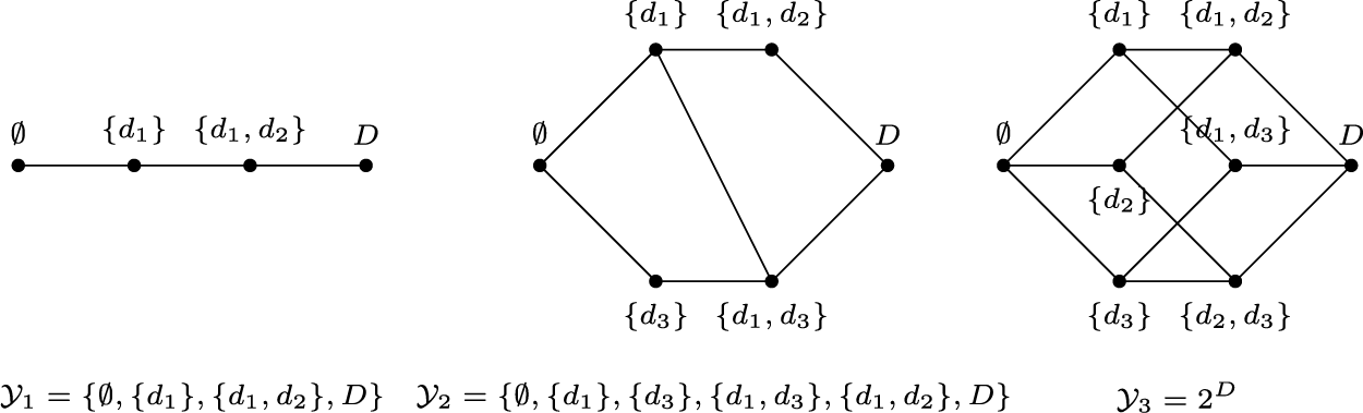


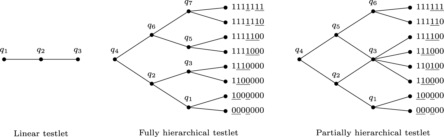


 Open access