


Introduction
Accurate characterization of the thermal state of present-day ice sheets is essential for improving projections of future ice flow and mass loss (Pattyn, Reference Pattyn2010; Seroussi and others, Reference Seroussi2013). Across both Antarctica and Greenland, ice dynamics depend strongly on englacial and basal temperatures: englacial temperature affects ice deformation, while basal melt influences sliding (Budd and Jacka, Reference Budd and Jacka1989; Engelhardt, Reference Engelhardt2004; Mantelli and others, Reference Mantelli, Haseloff and Schoof2019; Ranganathan and Minchew, Reference Ranganathan and Minchew2024). Therefore, better constraints on the thermal structure of ice sheets are critical for improving projections of future ice sheet mass contribution to global sea-level change (Dawson and others, Reference Dawson, Schroeder, Chu, Mantelli and Seroussi2022; Law and others, Reference Law, Christoffersen, MacKie, Cook, Haseloff and Gagliardini2023).
Despite its importance, the temperature distribution within the Antarctic and Greenland ice sheets remains poorly constrained. Modeled temperature fields show large discrepancies; for example, basal temperatures differ by more than 10 K among leading models in the Ice Sheet Model Intercomparison Project 6 (ISMIP6) (Seroussi, Reference Seroussi2019). This uncertainty is particularly pronounced in interior regions, where the boundaries between likely frozen and thawed beds are poorly defined across much of Greenland (MacGregor and others, Reference MacGregor2022) and largely unknown in vast subglacial basins of East Antarctica (Pelle and others, Reference Pelle, Morlighem and McCormack2020; Dawson and others, Reference Dawson, Schroeder, Chu, Mantelli and Seroussi2024), which hold the greatest volumes of grounded ice.
These discrepancies underscore the lack of observational constraints. Borehole thermometry provides the most accurate measurements of ice sheet temperature, but such data are sparse and geographically limited due to logistical challenges operating in remote polar environments (Løkkegaard and others, Reference Løkkegaard2023; Talalay, Reference Talalay2023). Most boreholes are located in the interior and along ice divides, and many do not reach the bed. Although essential ground-truth observations, boreholes are insufficient for constraining large-scale ice sheet models.
In contrast, radar sounding data provide extensive spatial coverage and offer indirect inference of temperature through signal attenuation. As electromagnetic waves propagate through glacial ice, they lose energy due to intrinsic absorption, which increases with temperature (Matsuoka and others, Reference Matsuoka, MacGregor and Pattyn2012). This temperature dependence causes radar signals to attenuate more rapidly in warmer ice, making attenuation rate a useful proxy for englacial temperature. Correcting for englacial attenuation also improves interpretation of the basal thermal state and the ability to distinguish thawed from frozen beds, enabling more reliable separation of variations in bed reflectivity from those caused by signal loss within the ice (Catania and others, Reference Catania, Conway, Gades, Raymond and Engelhardt2003; Jacobel and others, Reference Jacobel, Welch, Osterhouse, Pettersson and MacGregor2009). Despite the broad coverage of radar surveys, depth-averaged attenuation estimates spanning the full ice column remain limited. In Antarctica, only the Amundsen Sea Embayment is extensively mapped in this way (Chu and others, Reference Chu2021). In Greenland, radar-derived attenuation estimates are more widespread, but these estimates exclude the deepest and warmest ice near the bed (MacGregor and others, Reference MacGregor2015b).
Englacial radar attenuation rates derived directly from radar data are commonly estimated using one of two general approaches (Hills and others, Reference Hills, Christianson and Holschuh2020): (1) quantifying signal loss from the decay of internal reflections along individual radar traces (e.g., MacGregor and others, Reference MacGregor2015a), and (2) inferring attenuation by correlating bed echo power with ice thickness across multiple traces (e.g., Schroeder and others Reference Schroeder, Seroussi, Chu and Young2016). However, the former approach is ineffective in regions with extensive echo-free zones, where internal reflections are absent or heavily disrupted and poorly imaged. The latter approach assumes that bed echo power varies primarily with ice thickness, but this assumption fails where ice is thick and the bed is flat, as there is insufficient thickness variability and bed echoes are often weak due to high attenuation. It may also be violated where there are mixed wet and dry bed conditions, introducing additional variation in bed echo power. These limitations underscore the need for a method to estimate full-column attenuation rates that is not limited by the local variability in ice thickness or quality of radiostratigraphy.
Here we introduce the spectral ratio method as a robust alternative for estimating radar attenuation rates in ice sheets that is unaffected by the limitations of the above-mentioned methods. Unlike time-domain methods that track amplitude decay with depth, the spectral ratio approach analyzes changes in the signal’s frequency content between shallow and deeper reflectors. Originally developed for seismic exploration (Rickett, Reference Rickett2006) and then adapted for ground-penetrating radar (e.g., Harbi and McMechan, Reference Harbi and McMechan2012), this method shares conceptual similarities with multi-frequency radar techniques now being explored in terrestrial and planetary sounding (Pettinelli and others, Reference Pettinelli2015; Broome and others, Reference Broome, Schroeder and Johnson2023; Eide and others, Reference Eide, Casademont, Berger, Dypvik, Shoemaker Thackston and Hamran2023). In this study, we demonstrate the application of the spectral ratio method to estimate attenuation rates from ice sheet radar sounding data and compare our results to attenuation rates derived from deep ice borehole observations, model output and other radar-based techniques.
Data and methods
We apply the spectral ratio method to airborne radar sounding data from the interiors of the Greenland and Antarctic ice sheets. The resulting depth-averaged attenuation rate estimates constitute our primary dataset. To evaluate the method’s performance, we compare these results to attenuation estimates from other radar-based techniques, borehole observations and numerical thermal models. All datasets were obtained from prior studies and publicly available repositories.
Radar surveys and processing
We analyze two airborne radar surveys acquired by the University of Kansas Center for Remote Sensing and Integrated Systems (CReSIS) using the Multichannel Coherent Radar Depth Sounder (MCoRDS) system (Rodriguez-Morales and others, Reference Rodriguez-Morales2014) (Fig. 1). The first survey, flown on 30 March 2012, spans the central ice divide of Greenland (segment 20120330_03, frames 001–029). The second, flown on 27 November 2013, crosses the interior of East Antarctica (segment 20131127_01, frames 005–070). These surveys were selected because they intersect multiple deep ice boreholes and include extensive englacial reflectors, enabling comparisons with both boreholes and internal reflection-based attenuation estimates.
Study areas in (a) Greenland and (b) Antarctica. Radar survey lines (black) and borehole locations (red dots) are shown overlaid on bed elevation maps from BedMachine Version 5 (Morlighem and others, Reference Morlighem2022) and Bedmap3 (Pritchard and others, Reference Pritchard2024), respectively. These datasets form the basis for the attenuation analysis.

Both surveys were conducted using the NASA P-3 aircraft as part of Operation IceBridge (MacGregor and others, Reference MacGregor2021). The MCoRDS system features 15 receive channels and seven transmit channels, with a total transmit power of about 1050 W, equaling 150 W per channel (300 W on the center channel, but due to poor gain its nadir-directed power is equivalent to about 150 W). The system operates at a center frequency of 195 MHz with a 30 MHz bandwidth.
We process the raw radar data using the CReSIS Open Polar Radar ‘qlook’ processor (Open Polar Radar, 2024), which corrects for hardware effects, removes coherent noise, coherently sums receive channels and applies pulse compression using a synthetic reference waveform. To preserve the frequency content required for spectral analysis, we disable the final incoherent averaging step. By default, the qlook processor applies a Tukey window in the time domain and a Hanning window in the frequency domain to reduce sidelobes and spectral leakage. We evaluate the effect of disabling these windows and find minimal impact on our results, which rely on the ratio of amplitude spectra. However, because the Hanning window modifies the surface and bed spectra, we omit it in our processing even though the ratio remains unchanged. Figure S1 (Supplementary Material) shows example slope fits for each windowing configuration.
The next stage of the processing consists of applying several quality control steps. Surface and bed picks are refined by selecting the peak power within a window centered on the original CReSIS picks. We exclude flight segments where aircraft turns exceed 2 $^\circ$ km $^{-1}$ and where ice thickness is less than 500 m (MacGregor and others, Reference MacGregor2015b; Chu and others, Reference Chu2021). To ensure a high signal-to-noise ratio (SNR), we exclude radar traces where the bed return power is less than 10 dB above the noise floor (Figs. 3b and 4b) (Chu and others, Reference Chu2021). This SNR threshold is applied in the frequency domain using the lowest frequency quartile within the signal bandwidth and removes approximately 25% of all radar traces for both surveys. The 10 dB threshold was chosen as a conservative criterion to ensure that only high-quality traces are included in this first large-scale application of the method.
Spectral ratio method for estimating attenuation rates
We estimate depth-averaged radar attenuation rates using the spectral ratio method applied to the processed airborne radar sounding data. Originally developed for seismic exploration (Rickett, Reference Rickett2006), this method quantifies attenuation by analyzing the frequency-dependent decay of wave amplitudes with depth. While previously applied to ground-penetrating radar (e.g., Harbi and McMechan, Reference Harbi and McMechan2012), this study presents its first application to airborne radar sounding surveys of ice sheets.
In our application, the method exploits the fact that higher-frequency components within the radar signal bandwidth experience greater attenuation over a given propagation distance through ice, compared to lower-frequency components. This formulation assumes that the quality factor,  $Q$, which expresses the ratio of stored to dissipated energy per cycle, is constant across the radar signal bandwidth, which we empirically show to be reasonable for the frequency range used in this study. However, this assumption should be re-evaluated if the method is applied across wider or different frequency ranges, due to the apparent frequency dependence of attenuation over broader bands (Grimm and others, Reference Grimm, Stillman and MacGregor2015; MacGregor and others, Reference MacGregor2015b). The assumption that $Q$ remains constant across frequencies implies that each frequency component loses the same fraction of energy per wavelength. As a result, over any fixed propagation distance, higher-frequency components traverse more wavelengths and undergo greater cumulative energy loss.
The amplitude decay with depth can be modeled as
 \begin{equation}
a(\omega,\tau_2) = a(\omega,\tau_1)\, e^{- \alpha v \Delta \tau},
\end{equation}
\begin{equation}
a(\omega,\tau_2) = a(\omega,\tau_1)\, e^{- \alpha v \Delta \tau},
\end{equation}where  $a(\omega,\tau)$ is the amplitude spectrum at a given travel time $\tau$, $\Delta\tau = \tau_2 - \tau_1$, $\omega$ is the angular frequency and $\alpha$ is the attenuation constant. In practice, measured spectra are scaled by various physical and nonphysical effects such as geometric spreading, transmission and reflection losses and imperfect gain compensation. To account for these, we define a scaled amplitude
 \begin{equation}
A(\omega,\tau_2) = a(\omega,\tau_2)\, e^{\beta(\tau)},
\end{equation}
\begin{equation}
A(\omega,\tau_2) = a(\omega,\tau_2)\, e^{\beta(\tau)},
\end{equation}with  $\beta(\tau_1) = 0$. Equation 1 then becomes
 \begin{equation}
A(\omega,\tau_2) = A(\omega,\tau_1)\, e^{\Delta \beta}\, e^{- \alpha v \Delta \tau},
\end{equation}
\begin{equation}
A(\omega,\tau_2) = A(\omega,\tau_1)\, e^{\Delta \beta}\, e^{- \alpha v \Delta \tau},
\end{equation}where  $\Delta \beta = \beta(\tau_2) - \beta(\tau_1)$ represents frequency-independent amplitude scaling due to spreading, reflection, transmission losses and other effects. The phase velocity $v$ is given by $v = c / \sqrt{\epsilon_r}$, where $c$ is the speed of light in a vacuum and $\epsilon_r$ is the real part of the relative permittivity of ice.
For a low-loss dielectric such as ice, where the loss tangent  $\tan\delta \ll 1$, the attenuation constant can be approximated as
 \begin{equation}
\alpha \approx \frac{\omega}{2v} \tan\delta.
\end{equation}
\begin{equation}
\alpha \approx \frac{\omega}{2v} \tan\delta.
\end{equation} Since the quality factor is defined as  $Q = 1 / \tan\delta$, Equation 4 becomes
 \begin{equation}
\alpha \approx \frac{\omega}{2vQ}.
\end{equation}
\begin{equation}
\alpha \approx \frac{\omega}{2vQ}.
\end{equation}Taking the natural logarithm of the amplitude ratio from Equation 3, we obtain
 \begin{equation}
\ln \left[\frac{A(\omega,\tau_2)}{A(\omega,\tau_1)}\right] = \Delta \beta - \alpha v \Delta \tau,
\end{equation}
\begin{equation}
\ln \left[\frac{A(\omega,\tau_2)}{A(\omega,\tau_1)}\right] = \Delta \beta - \alpha v \Delta \tau,
\end{equation}and substituting Equation 5, we get
 \begin{equation}
\ln \left[\frac{A(\omega,\tau_2)}{A(\omega,\tau_1)}\right] = \Delta \beta - \frac{\omega \Delta \tau}{2Q}.
\end{equation}
\begin{equation}
\ln \left[\frac{A(\omega,\tau_2)}{A(\omega,\tau_1)}\right] = \Delta \beta - \frac{\omega \Delta \tau}{2Q}.
\end{equation} This equation describes the spectral ratio method of attenuation estimation (Rickett, Reference Rickett2006). A least-squares fit to the logarithm of the amplitude ratio as a function of angular frequency yields a slope proportional to  $Q^{-1}$ and an intercept equal to $\Delta \beta$.
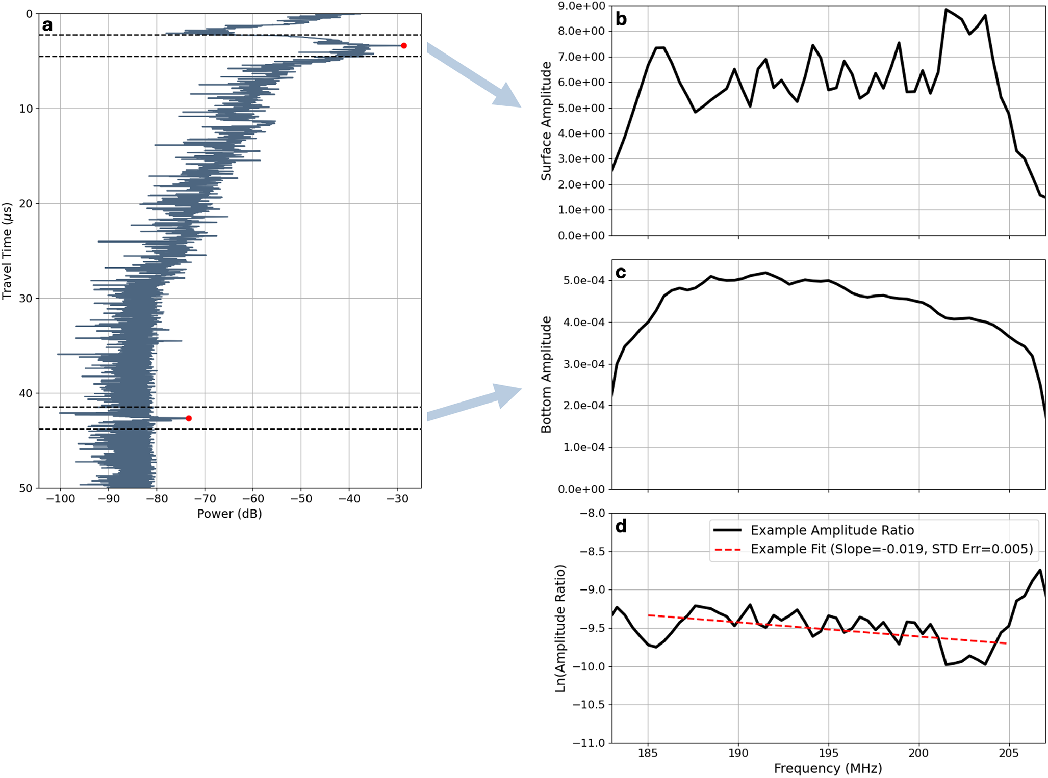
Implementation
For each radar trace, we calculate amplitude spectra using windowed fast Fourier transforms (FFTs) centered on the surface and bed picks. A 256-sample, 2.3  $\mu$s time window is applied around each pick (Figs. 2a, 3a and 4a) to produce the surface and bed spectra, $ A(\omega, \tau_1) $ and $ A(\omega, \tau_2) $, respectively (Fig. 2b and c). We then calculate the natural logarithm of their ratio to estimate the spectral slope (Equation 7), which is proportional to $ Q^{-1} $. To reduce noise and stabilize slope estimates, we apply a moving average over 800 traces (approximately 15 km of along-track distance). The linear least-squares fit is performed over the 185–205 MHz frequency range, avoiding edge-related spectral artifacts (Fig. 2d). We also compute the standard error of the fitted slope from the covariance matrix returned by the polynomial fit. This error serves as a valid uncertainty metric, as the slope estimates are approximately normally distributed.
Spectral ratio method. (a) Time-domain radar trace with FFT windows (black dashed lines) centered on the surface and bed picks (red dots), using a window size of 256 samples. (b) and (c) Amplitude spectra for the surface and bed windows, respectively. (d) Log of the amplitude ratio (bed divided by surface) with a linear fit (red dashed line) applied across the 185–205 MHz band.

We apply several quality control steps to remove unreliable slope estimates. First, we exclude traces with poorly constrained fits based on the slope standard error, which effectively filters out outliers. We also exclude positive slope values, which correspond to nonphysical negative attenuation rates. While negative apparent attenuation could theoretically occur if scattering dominates over intrinsic attenuation, this is not expected over the depth intervals analyzed here. Enforcing positive slope values is therefore a reasonable constraint (Rickett, Reference Rickett2006).
Conversion to attenuation rate
Using the fitted slope, we compute the attenuation constant  $ \alpha $ from $ Q $ via Equation 5, assuming a constant phase velocity $ v = c / \sqrt{\epsilon_r} $ and a center frequency of 195 MHz. This formulation assumes that attenuation is dominated by intrinsic losses. We then convert $ \alpha $, expressed in nepers per meter, to decibels per kilometer using
 \begin{equation}
\overline{N_a} = -20 \log_{10}(e) \cdot \alpha \cdot 1000 \approx -8686 \, \alpha.
\end{equation}
\begin{equation}
\overline{N_a} = -20 \log_{10}(e) \cdot \alpha \cdot 1000 \approx -8686 \, \alpha.
\end{equation} This yields the one-way, depth-averaged attenuation rate  $ \overline{N_a} $. To estimate the uncertainty in $ \overline{N_a} $, we propagate the slope standard error through the full attenuation model using first-order uncertainty analysis. Both the one-way, depth-averaged attenuation rate and associated uncertainty are shown in Figures 3c and 4c.
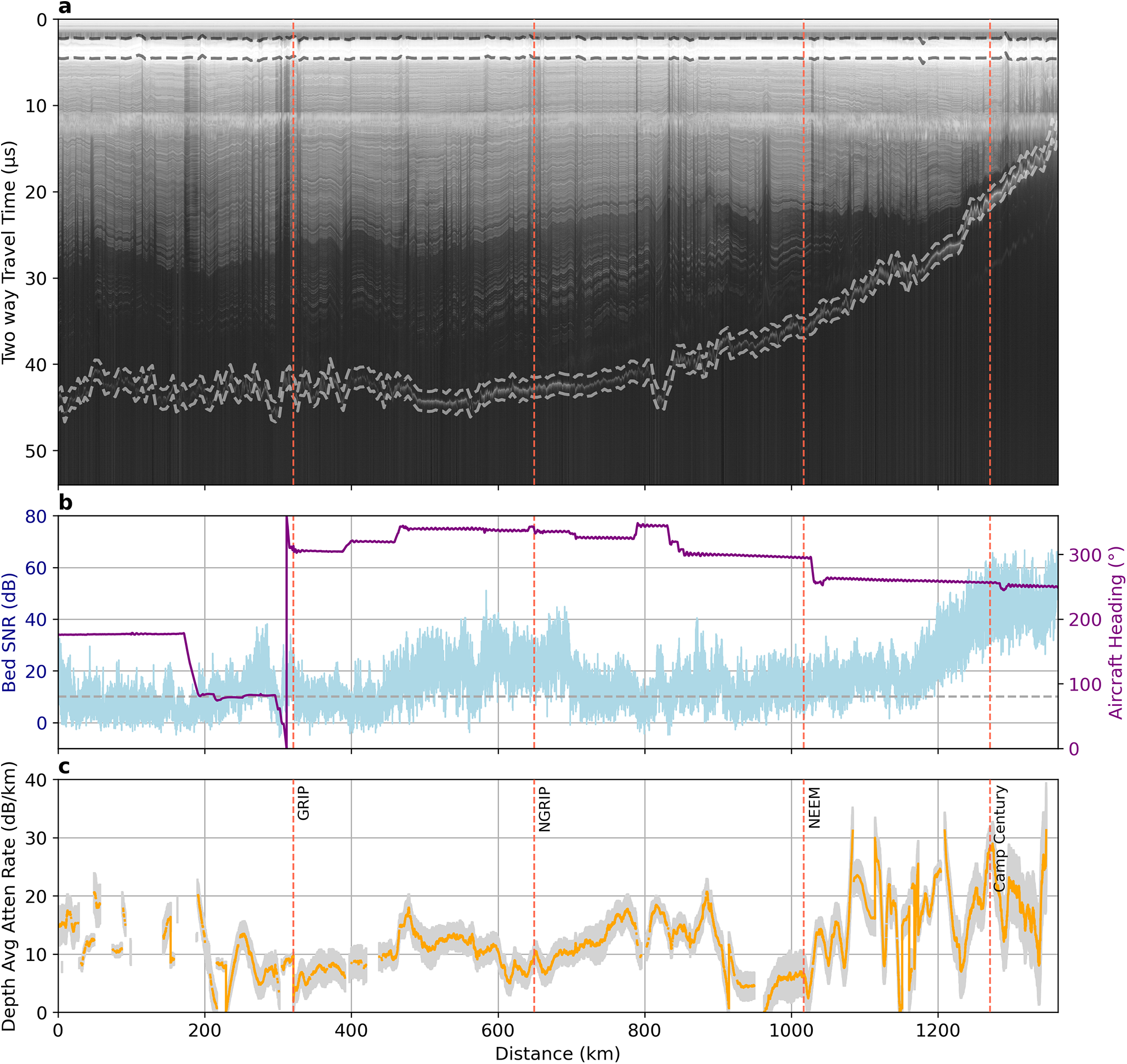
(a) Radargram from the Greenland transect showing the FFT windows (dashed lines) centered on the surface and bed reflections, using a 256-sample window. (b) Signal-to-noise ratio (SNR) of the bed reflection shown in light blue and aircraft heading along the transect shown in purple. The horizontal dashed line marks the 10 dB SNR cutoff. (c) One-way depth-averaged attenuation rate and the uncertainty shown in gray. Gaps indicate where attenuation estimates fail to meet quality thresholds. Red vertical dashed lines show where the survey crosses borehole locations.

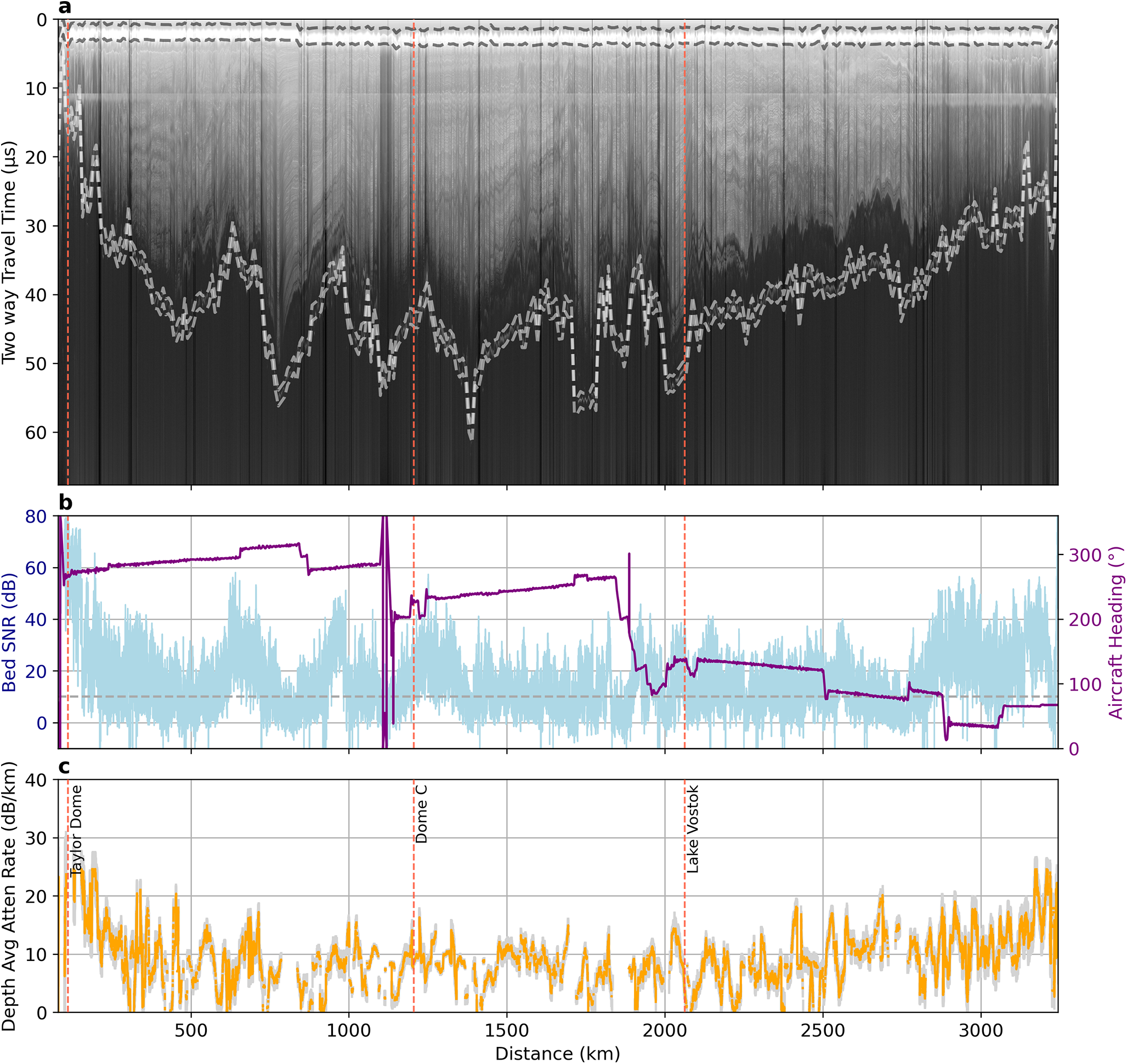
Same as Figure 3, but for the East Antarctica survey.

We exclude attenuation rate estimates that fall more than two standard deviations from the mean of all attenuation rates along the survey. This filtering step reduces the influence of statistical outliers that may arise from spectral noise, poor-quality radar traces or processing artifacts. Because the attenuation rate distribution is approximately Gaussian (Supplementary Material Fig. S3), this two-sigma criterion represents a conservative approach. It retains the majority of physically plausible estimates while removing extreme and lower-confidence values, consistent with standard practice in noisy geophysical datasets.
We assess the sensitivity of the method to three parameters (FFT window length, smoothing window size and the frequency range used for slope fitting) and found that our results are robust to these choices. Attenuation estimates show minimal variation when using window lengths of 128, 256 or 512 samples (Supplementary Material Fig. S2). Similarly, moderate changes in the smoothing window length have little effect (Supplementary Material Fig. S4). Varying the fitting band around the central 195 MHz can yield local differences exceeding 5 dB km $^{-1}$, but these do not alter the broad-scale attenuation pattern (Supplementary Material Fig. S5). We attribute these local variations to spectral noise, which has a greater proportional influence when the fitting is performed over a narrower frequency band. For this reason, we consider using the widest possible frequency window to be the most stable and reliable approach, consistent with findings from spectral ratio analyses in seismology (Tonn, Reference Tonn1991).
Adaptive fitting method for calculating attenuation rates
For comparison results, we also apply the adaptive fitting technique developed by Schroeder and others (Reference Schroeder, Seroussi, Chu and Young2016) to estimate one-way depth-averaged attenuation rates for both radar surveys. This method calculates attenuation by correlating variations in ice thickness with bed echo power, assuming that power loss is primarily due to intrinsic englacial attenuation.
To ensure robust estimates, we follow the correlation-based criteria defined by Schroeder and others (Reference Schroeder, Seroussi, Chu and Young2016). For each location along the radar transect, we expand the fitting window iteratively until the following three conditions are met: (a) the initial correlation coefficient between ice thickness and bed echo power is high ( $C_0 \ge 0.5$), indicating a strong linear dependence; (b) the minimum magnitude of the correlation coefficient within the window is low ( $C_m \le 0.01$), implying that the attenuation correction successfully flattens the power–thickness relationship; and (c) the radiometric resolution at the correlation minimum is $\le 1$ dB km $^{-1}$ for $C_w = 0.1$, ensuring the fitted attenuation rate is well resolved. If these criteria are not satisfied within a 10 km fitting radius, the method does not return an attenuation estimate for that location. This filtering ensures that only statistically reliable and physically interpretable attenuation rates are retained for comparison.
Layer-based method for calculating attenuation rates
We also estimate radar attenuation rates using the layer-based method developed by MacGregor and others (Reference MacGregor2015b). This approach relies on mapped internal radar reflections and analyzes the depth-dependent decay of radar power associated with those reflectors. For each traced reflector, received power is extracted, geometric and system gain corrections are applied and signal strength is compared against two-way travel time. The slope of the logarithmic decay in power with depth provides an estimate of the englacial attenuation rate. This method returns a depth-averaged rate over a variable depth range determined by the positions of the traced reflectors.
We make two modifications to the implementation described by MacGregor and others (Reference MacGregor2015b). First, we now use the geometrically corrected reflection powers ( $P_{rc}'$) from individual traced reflections to calculate the best-fit depth-averaged attenuation rate, rather than using interval differences ( $\Delta P_{rc}'$) between these reflections. This adjustment also simplifies subsequent uncertainty estimation. Second, we introduce a bias correction step to the $P_{rc}'$ values to address the assumption of vertically uniform layer reflectivity that is necessary for this method. This second correction effectively switches the assumption of vertical uniformity in reflectivity to that of horizontal uniformity. To accomplish this bias correction, we calculate the depth-averaged attenuation rate for the entire segment following MacGregor and others (Reference MacGregor2015b) and the first modification described above. Then, for each traced reflection, we bin its difference between the observed $P_{rc}'$ values and those ‘predicted’ by the inferred depth-averaged attenuation rate. If a given reflection has a statistically significant non-zero bias (Student’s $t$-test at 95% confidence), that bias is recorded. After the apparent reflectivity bias of all traced reflections is determined, the $P_{rc}'$ values are corrected for these biases and the attenuation rate is recalculated along the entire segment. Following these modifications, we recalculate attenuation rates and radar-inferred temperatures at locations where radar surveys intersect boreholes. The explained variance ( $r^2$) between radar- and borehole-derived temperatures improves from 0.85 to 0.90, primarily due to the first modification.
Although a second version of Greenland’s radiostratigraphy is now available (MacGregor and others, Reference MacGregor, Fahnestock, Paden, Li, Harbeck and Aschwanden2025), we use the first version (MacGregor and others, Reference MacGregor2015a) because it includes traced reflections for all the frames used in the spectral ratio method. For Antarctica, we use reflections traced by Cavitte and others ( Reference Cavitte2016); Reference Cavitte2021) and extend them along the survey using the method described by MacGregor and others (Reference MacGregor, Fahnestock, Paden, Li, Harbeck and Aschwanden2025) to trace additional reflections where visible.
Borehole-derived attenuation rates
We derive comparison attenuation rates using data from the seven borehole locations that intersect the radar flight lines (Fig. 1). In Antarctica, these include Taylor Dome, Dome C and Lake Vostok. In Greenland, these include GRIP, NorthGRIP, NEEM and Camp Century. Appendix A provides additional details on the data sources, dielectric properties and full attenuation profiles for each location.
Attenuation rates are estimated from the ice conductivity using borehole temperature profiles and ice core chemistry data shown in Figures 5 and 6. Where chemistry data is not available, we use dielectric profiling (DEP) data, which has been shown to be a robust proxy for total conductivity (Zirizzotti and others, Reference Zirizzotti, Cafarella, Urbini and Baskaradas2014; Culberg and Schroeder, Reference Culberg and Schroeder2021). Since DEP measures total conductivity, we cannot separate the contributions from different impurity species at those locations.
(a) Depth-averaged one-way attenuation rate estimates along the Greenland radar survey, using spectral ratio, adaptive fitting, layer-based and ISSM-derived methods, compared with intersecting borehole values. We also plot smoothed versions of the radar-derived attenuation rates to aid visual interpretation over the  $ \gt $1200 km transect. (b) Ice thickness along the same survey line.

Conductivity is modeled at the high frequency limit (suitable for low loss dielectrics such as ice) assuming an Arrhenius-form temperature dependence and linear chemical impurity dependence (Matsuoka and others, Reference Matsuoka, MacGregor and Pattyn2012; MacGregor and others, Reference MacGregor2015b):
 \begin{equation}
\sigma_\infty = \sum_{i=0}^3 \sigma_i^0 C_i\, \exp\left[-\frac{E_i}{k} \left(\frac{1}{T(z)} - \frac{1}{T_r} \right) \right],
\end{equation}
\begin{equation}
\sigma_\infty = \sum_{i=0}^3 \sigma_i^0 C_i\, \exp\left[-\frac{E_i}{k} \left(\frac{1}{T(z)} - \frac{1}{T_r} \right) \right],
\end{equation}where  $\sigma_i$ is the conductivity, $C_i$ is the radar-effective concentration and $E_i$ is the activation energy for species $i$.
$i$.  $T(z)$ is the measured temperature profile, $T_r = 251$ K is the reference temperature and $k$ is the Boltzmann constant. The first term is the pure ice contribution, where $\sigma_0^0$ is the pure-ice conductivity ( $i = 0$). The next three terms are the dominant chemical impurities in polar ice sheets that affect ice conductivity, sea salt chloride (ssCl $^-$), acids (H $^+$) and ammonium (NH $_4^+$).
At sites with chemistry measurements (Lake Vostok, Taylor Dome, GRIP), we calculate impurity concentrations following MacGregor and others (Reference MacGregor2007) and use that to calculate all terms in Equation 9. We assign a uniform uncertainty of 0.5  $\mu$M to [H $^+$], [ssCl $^-$] and [NH $_4^+$], also following MacGregor and others (Reference MacGregor2007). Assuming no covariance between inputs, we estimate the uncertainty in total conductivity $\tilde{\sigma}_\infty$ via standard error propagation. At sites with only DEP data (Dome C, NorthGRIP, NEEM, Camp Century), we estimate the total $\sigma^0 C$ from the DEP observations and use that as an input to compute $\sigma_\infty$.
The one-way attenuation rate is computed from its proportionality to the high-frequency limit of electrical conductivity (Winebrenner and others, Reference Winebrenner, Smith, Catania, Conway and Raymond2003; MacGregor and others, Reference MacGregor2007):
 \begin{equation}
N_a(\sigma) = \frac{1000 \cdot (10 \log_{10} e)}{c \epsilon_0 \sqrt{\epsilon_r}} \, \sigma_\infty,
\end{equation}
\begin{equation}
N_a(\sigma) = \frac{1000 \cdot (10 \log_{10} e)}{c \epsilon_0 \sqrt{\epsilon_r}} \, \sigma_\infty,
\end{equation}where  $\epsilon_0$ is the permittivity in a vacuum and $\epsilon_r$ is the real part of the relative permittivity of ice. Uncertainty in $N_a$ is propagated from the uncertainty in $\sigma_\infty$. Because electrical conductivity varies with depth, we apply Equation 10 point-wise to obtain a depth-resolved attenuation rate profile $N_a(z)$. We then compute the one-way depth-averaged attenuation rate as the cumulative mean of this profile from the surface to a depth $z$ (up to the ice thickness $H$):
$H$):
 \begin{equation}
\overline{N_a} = \frac{1}{z} \int_0^{0 \leq z \leq H} N_a(z) \, dz.
\end{equation}
\begin{equation}
\overline{N_a} = \frac{1}{z} \int_0^{0 \leq z \leq H} N_a(z) \, dz.
\end{equation}We report the depth-averaged attenuation rate over the full ice column in Table 2 for each borehole location, with full profiles shown in Figures A1 and A2.
Ice sheet model derived attenuation rates
To provide comparison between models and observations, we also derive attenuation rates from thermal model output. We use model output from the Ice-sheet and Sea-level System Model (ISSM) for both Antarctica and Greenland, and use the temperature field to derive one-way depth average attenuation rates along both radar tracks. For Antarctica, the ISSM thermal model output comes from Dawson and others (Reference Dawson, Schroeder, Chu, Mantelli and Seroussi2022). For Greenland, the ISSM thermal model output comes from Seroussi and others (Reference Seroussi2013). To derive attenuation rates from depth-averaged temperatures, we use the same Arrhenius relationship (Equation 9) that we used for the borehole analysis, with averaged molar impurities and activation energies. ISSM-derived temperature profiles are also compared to borehole temperature profiles in Figure S6 (Supplementary Material).
Results
Figures 3c and 4c show the attenuation rates produced using the spectral ratio method. These results extend full-column attenuation coverage into new regions of Greenland and Antarctica, demonstrating the method’s ability to extract additional information from radar sounding data. The method provides high spatial coverage, returning attenuation rate estimates for over 85% of each survey transect (Table 1).
Summary statistics for one-way attenuation rate estimates from the spectral ratio, layer-based and adaptive methods. Mean and standard deviation values for the entire radar transects are reported. Coverage refers to the percentage of each radar transect with valid attenuation estimates returned.

We evaluate the method’s performance by comparing its results with those from other radar-based approaches, thermal model predictions and borehole-derived estimates. Among radar-based techniques, the spectral ratio method achieves nearly the same coverage (percentage of track with valid attenuation estimates) as the layer-based method across East Antarctica and Greenland. It also returns the highest mean attenuation rates, suggesting improved sensitivity to elevated attenuation near the base of the ice column (Table 1). Its broader spread in estimates may reflect both responsiveness to local ice conditions and residual noise (e.g., scattering from surface or basal roughness). For both surveys, attenuation rates follow a lognormal distribution (Supplementary Material Fig. S3).
Along the Greenland transect, the spectral ratio method yields slightly higher mean attenuation rates than the layer-based method (13.0 vs. 11.6 dB km $^{-1}$; Table 1) and has greater spatial variability (Fig. 5a). The largest discrepancy occurs between NorthGRIP and NEEM, where spectral ratio results show elevated attenuation rates between the boreholes but lower values at the borehole sites relative to the other methods. The adaptive method does not converge along this transect because of its core assumption, that the bed echo power scales with the thickness of the ice, not being satisfied.
Along the East Antarctic transect, radar-derived attenuation rate estimates appear noisier, but the transect is more than twice as long as the Greenland line, compressing the  $x$-axis in Figure 6. The normalized variation in spectral ratio results is nearly identical between the two transects (Table 1), showing that the variation is actual similar for both surveys. As in Greenland, the spectral ratio method yields slightly higher average values overall compared to the layer-based method (9.6 vs. 7.4 dB km $^{-1}$; Table 1). The layer-based method does not return values where internal layers are discontinuous, especially at the beginning and end of the transect where ice thickness changes rapidly. The adaptive method only converges over small sections, such as near Taylor Dome and local topographic highs at the edges of the Wilkes Basin. The ISSM-derived attenuation estimates show similar large-scale spatial patterns, however in some areas (e.g., 500–1000 km along-track), spectral-ratio-based and ISSM-derived estimates exhibit similar trends but are offset laterally by 50 to 100 km.
Same as Figure 5, but for the East Antarctic survey. Note that the adaptive fitting method converges along portions of this survey and is also shown.

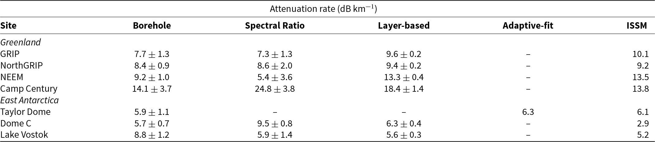
Comparisons with the seven borehole-derived attenuation rates show that the spectral ratio method agrees within uncertainty bounds at four of six locations where spectral estimates are available (Table 2). The most significant mismatch occurs at Camp Century, where the spectral estimate exceeds the borehole-derived value. The layer-based method tends to slightly overestimate attenuation at the boreholes relative to the borehole estimates, despite having lower average attenuation rates over the entire surveys (Table 1). Thermal model predictions from ISSM underestimate attenuation at Dome C and Lake Vostok relative to both radar-based methods and borehole results.
Depth-averaged one-way attenuation rates and their uncertainty estimated at the seven borehole sites using multiple methods. The uncertainty estimates for the spectral ratio method and layer-based method are 1-sigma standard error.

Discussion
Performance across variable surface and subglacial environments
The spectral ratio method produces attenuation rates consistent with borehole observations, while also providing broader spatial coverage and finer along-track resolution than other techniques. Unlike layer-based or adaptive methods, which require continuous internal reflectors or a strong correlation between bed power and ice thickness, the spectral ratio approach can be applied across radargrams with limited layering or uniform ice thickness, while still yielding variability along track that is comparable to that of layer-based estimates. Because the method relies on the change in spectral shape between the surface and bed, rather than absolute bed power, it is much less sensitive to whether the bed is wet or dry, and thus avoids the bias that thickness–power regressions can experience in the presence of subglacial water.
Our analysis also shows that the method remains valid even when the surface return spectrum is not perfectly flat. For example, Figure 2b shows a subtle shift of surface power toward higher frequencies. In Greenland, firn layers, ice lenses and percolation features can generate near-surface reflectors, and in many places along our survey we observe second returns within the surface FFT window. However, these secondary returns are not spatially correlated with deviations in the surface spectral shape (Supplementary Material Fig. S7), indicating that surface spectral variability is not driven by near-surface reflections. The subtle shift towards higher frequencies may indicate shallow scattering, although the bandwidth corresponds to a small relative change in wavelength, only a few tens of centimeters, so signal interactions with scatterers should not change strongly across this range. The variation could also relate to system-driven characteristics of the transmitted waveform and knowing the amplitude spectrum of the waveform could help isolate these contributions. However, crucially, the spectral ratio method does not require the transmitted waveform or surface spectrum to be flat. Because both the surface and bed returns share the same system imprint and both travel through the surface, their ratio isolates the spectral shift introduced by propagation through the entire ice column. This capability enables attenuation mapping across regions where conventional radar-based approaches fall short and provides new observational constraints that have not previously been available at this scale from radar sounding data.
Patterns in attenuation rate and implications for thermal regime
On average, across both ice sheets, the spectral ratio method reports higher depth averaged attenuation than the layer-based method (Table 1). In central Greenland, this difference is largest between NorthGRIP and NEEM from  $\sim$700–900 km along-track distance, and in East Antarctica values are especially elevated near Dome C and at $\sim$1500 km along-track distance (Figs. 5a and 6a). The spectral ratio method produces an estimate of attenuation that captures the entire ice column because it compares spectral content between surface and bottom reflectors. In contrast, the depth-averaged attenuation estimates from the layer-based method only comes from internal reflections, so deepest part of the ice sheet, which is often either echo-free or simply not traced, is not captured by this method.
Since the deepest part of the ice column contains the largest temperature gradients and warmest ice, often reaching the pressure-adjusted melting temperature in interior basins, and can be enhanced by high geothermal heat flux (Lowe and others, Reference Lowe, Mather, Green, Jordan, Ebbing and Larter2023), this part of the column causes a disproportionately large amount of attenuation (Fig. 7a and b). Therefore, we interpret the higher depth-averaged attenuation reported by the spectral ratio method in the NorthGRIP to NEEM region in Greenland and the Dome C region in East Antarctica to capture attenuation from the warmer, deeper ice that the layer-based method is insensitive to. Figures S8 and S9 (Supplementary Material) show the stratigraphy and extent of the echo-free zone (defined as the zone between the deepest traced layer and the bed) and the attenuation rates and uncertainties from both methods in these regions of the Antarctica and Greenland profiles. The pattern of typically higher values from the spectral method, and its apparent relationship with the ‘echo-free zone’ support our argument that the spectral method’s apparent bias compared to the layer-based method is because the former method is also sensitive to the deepest part of the ice column.
Schematic showing how advection, conduction and basal boundary conditions influence ice sheet thermal structure and the resulting depth-averaged radar attenuation rate. (a and b) A scenario with variable ice thickness and only vertical conduction and advection (e.g., near an ice divide). (c and d) A scenario with a subglacial lake and heat loss associated with basal melting. (e and f) A glacier along-flow scenario with horizontal advection and frictional heating, and varying ice thickness. (g and h) An across-shear margin scenario with shear heating and frictional heating on the fast flowing side.

A method that is sensitive to the lower portion of the ice sheet column also has the potential to encode other signatures of thermal regime change. The schematics in Figure 7, which is based on simple one-dimensional thermal model scenarios, show expected attenuation rate signatures for different basal boundary conditions and flow regimes. A subglacial lake should cause a local dip in the depth averaged attenuation rate (Fig. 7c and d). In our results, the drop in spectral ratio derived attenuation rates near NEEM could indicate that basal melting is modulating the thermal structure there, leading to reduced vertical conduction in the ice column (e.g., Karlsson and others, Reference Karlsson2021). Alternatively, these attenuation features could arise from increased scattering or signal loss due to englacial reflections, particularly in the presence of large basal units or rough bed topography, both of which could influence amplitude spectra and are present in the area (Goossens and others, Reference Goossens, Sapart, Dahl-Jensen, Popp, El Amri and Tison2016; Jordan and others, Reference Jordan2017). Focused analysis at finer spatial resolution is needed to distinguish between thermal and scattering-related causes. The spectral ratio method also shows relative decreases in attenuation adjacent to Dome C and over parts of Lake Vostok. These features may reflect suppression of englacial temperature gradients due to basal meltwater (Fig. 7c and d). However, the spatial resolution of this study limits confident interpretation at these scales. Over Lake Vostok, the complex chemical environment further complicates the interpretation; the simple illustrative scenario shown in Figure 7c and d may not capture the complexity of the lake lid properties (MacGregor and others, Reference MacGregor, Matsuoka and Studinger2009; Winebrenner and others, Reference Winebrenner, Kintner and MacGregor2019). The more complex scenarios in Figure 7e through 7h also show that horizontal advection, shear heating or both can modify the attenuation signature. These mechanisms are present in fast-flowing regions and the spectral ratio method may therefore have power to detect thermal regime transitions associated with flow state changes.
Considerations for broader application
There are opportunities to further develop the spectral ratio method for use in thermal interpretation and ice sheet model calibration. For instance, the method can be extended to incorporate englacial reflectors in a tomography-style inversion to estimate a depth-resolved quality factor ( $Q$), similar to the approach in Rickett (Reference Rickett2006). This would enable retrieval of attenuation rates as a function of depth, potentially resolving finer-scale thermal variations such as zones of enhanced shear heating (e.g., Summers and others, Reference Summers, Schroeder, May and Suckale2024) or along-flow scenarios involving basal frictional heating and horizontal advection, as illustrated in Figure 7e–h.
While the spectral ratio method demonstrates broad applicability and strong potential, its performance is subject to several important considerations that influence accuracy and interpretation. To date, it has been applied only to airborne radar data from the MCoRDS system, which operates at a center frequency of 195 MHz with a 30 MHz bandwidth. Extending the method to other radar systems will require careful consideration of signal quality, system-specific frequency characteristics and processing pipelines. The method depends on measurable frequency-dependent attenuation; if the bandwidth is too narrow, spectral slope estimates may be undetectable relative to signal noise. In contrast, very wide bandwidths may challenge the assumption of a constant quality factor across the fitting window. At significantly higher or lower frequencies, dielectric behavior may deviate from the simple low-loss model used here, potentially requiring alternative formulations using Debye or Cole–Cole models (e.g., Fujita and others, Reference Fujita, Matsuoka, Ishida, Matsuoka, Mae and Hondoh2000; Grimm and others, Reference Grimm, Stillman and MacGregor2015). Across the frequency range of the system used in this study (180–210 MHz), MacGregor and others (Reference MacGregor2015b) inferred a  $\sim$2% increase in ice conductivity from 180 MHz to 210 MHz for Greenland, based on a comparison between radar-inferred and borehole temperatures. The magnitude of this frequency dependence was broadly consistent with inferences from dielectric spectroscopy of ice cores and previous wider bandwidth radar studies. However, for a more recent version of MCoRDS that operates between 150 and 520 MHz (Kjæ r and others, Reference Kjær2018; Arnold and others, Reference Arnold2020), the equivalent increase would be $ \gt $20%, which would likely require introducing an additional correction to the attenuation rates derived from the spectral ratio method.
Because attenuation rates represent integrated properties of the ice column, some degree of along-track smoothing is necessary to stabilize spectral slope estimates and suppress trace-level noise. However, overly aggressive smoothing can obscure meaningful spatial variations, particularly near thermal boundaries. The appropriate smoothing scale should reflect expected gradients in thermal structure as well as the radar system’s spatial resolution. In regions with complex bed topography or large variability in basal reflectivity, assumptions about locally uniform geometric spreading and transmission losses may break down, further biasing the estimated attenuation rate.
Finally, the method captures the total attenuation, which includes both intrinsic dielectric absorption and scattering. While smoothing can be used to emphasize the broader-scale intrinsic signal, small-scale scattering from disrupted stratigraphy or rough basal interfaces may still influence results. This effect is particularly relevant in dynamically complex areas such as shear margins, grounding zones or crevassed ice. Additional work is needed to assess the method’s sensitivity to scattering and to better distinguish the relative contributions of attenuation mechanisms. Thus, this method can be viewed as a powerful complement—rather than a complete replacement—for existing radar-based attenuation estimation techniques. It is valuable for extending and filling in spatial gaps where other methods fail and providing higher-resolution estimates and independent constraints.
Conclusion
We introduced a novel method for estimating radar attenuation through ice sheets using the frequency-dependent behavior of radar signal amplitudes. By applying the spectral ratio method to airborne radar surveys over central Greenland and East Antarctica, we demonstrate robust, depth-averaged attenuation rate estimates through the full ice column, including areas where traditional methods fail due to limited internal layering or uniform ice thickness.
Our results show good agreement with independent attenuation estimates derived from deep-borehole conductivity profiles, layer-based radar analysis and numerical thermal models. At the majority of the seven borehole locations, the spectral ratio estimates fall within uncertainty bounds of borehole measurements. Compared to alternative radar-based methods, the spectral ratio approach provides broader spatial coverage without sacrificing spatial resolution. It also offers improved sensitivity to attenuation in the lower ice column, supporting improved basal thermal characterization. This capability is critical, as the thermal state strongly influences ice viscosity, deformation and basal conditions, and yet remains one of the most poorly constrained aspects of ice sheet models.
The method’s flexibility and computational efficiency make it well suited for large-scale application across radar datasets that preserve the amplitude spectrum. It can also serve as a complement to existing techniques, providing estimates where layer-based or bed power correlation methods are not applicable and improving attenuation estimates in areas with sparse internal reflections. This study lays the foundation for more extensive attenuation mapping into previously inaccessible regions, providing a scalable approach to support both glaciological interpretation and large-scale ice sheet modeling.
Supplementary Material
The supplementary material for this article (Figs. S1–S9) can be found at https://doi.org/10.1017/jog.2026.10130.
Data
The raw radar data used in this study are available open source from the Open Polar Radar platform at https://data.cresis.ku.edu/data/raw_data/. The attenuation rates produced in this study are archived on Zenodo and are available at https://doi.org/10.5281/zenodo.18331054. The spectral ratio processing and analysis code was developed in Python, and the scripts used to generate the figures were run in Python and MATLAB R2025a. These are available at https://github.com/elizadawson/Dawson2026JOG.git.
Acknowledgements
We thank John Paden for providing access to the raw MCoRDS data and for his continued efforts to make the Open Polar Radar processing pipeline more accessible. We also acknowledge Reece Mathews and the full CReSIS and Open Polar Radar teams for their support in making this analysis possible. We thank the Associate Chief Editor and two anonymous reviewers for their thoughtful and constructive feedback.
E.J. Dawson was supported by the NOAA Climate and Global Change Postdoctoral Fellowship Program, administered by UCAR’s Cooperative Programs for the Advancement of Earth System Science (CPAESS) under the NOAA Science Collaboration Program award # NA23OAR4310383B. J. A. MacGregor was supported by the Internal Scientist Funding Model for NASA’s Cryospheric Sciences Program.
Appendix A. Borehole-derived attenuation rates
Figures A1 and A2 summarize the borehole datasets used to derive attenuation rates in this study. These figures show temperature profiles, one-way attenuation rates and corresponding depth-averaged values. Attenuation rates are calculated using the Arrhenius relationship (Equation 9), combining temperature measurements with impurity concentrations to estimate total electrical conductivity,  $\sigma_\infty$.
Figure A1: Temperature profiles, one-way attenuation rates and depth-averaged attenuation rates for Greenland boreholes. Top row (a–c): GRIP; second row (d–f): NorthGRIP; third row (g–i): NEEM; bottom row (j–l): Camp Century. Attenuation estimates are derived from temperature, chemistry and DEP data.

Temperature profiles, one-way attenuation rates and depth-averaged attenuation rates for Antarctic boreholes. Top row (a–c): Taylor Dome; second row (d–f): Dome C; bottom row (g–i): Lake Vostok. Attenuation estimates are derived from temperature, chemistry and DEP data.

For Greenland, we analyze data from four borehole sites: GRIP, NorthGRIP, NEEM and Camp Century. Temperature profiles are sourced from Løkkegaard and others (Reference Løkkegaard2023). Chemistry data for NorthGRIP and dielectric profiling (DEP) data for GRIP and NEEM come from MacGregor and others (Reference MacGregor2015b). At Camp Century, only temperature data are available.
In Antarctica, we include Taylor Dome, Dome C and Lake Vostok. Lake Vostok data are provided by MacGregor and others (Reference MacGregor, Matsuoka and Studinger2009); Taylor Dome data are compiled from (Mayewski and others, Reference Mayewski1996; Morse, Reference Morse1997; Stager and Mayewski, Reference Stager and Mayewski1997; Steig and others, Reference Steig2000); Dome C data are drawn from (EPICA community members, 2004; Stauffer and others, Reference Stauffer, Flückiger, Wolff and Barnes2004; Buizert and others, Reference Buizert2021).
At each site, we show the total attenuation rate and its components from pure ice (temperature-driven), sea-salt chloride (ssCl $^-$) and acids (H $^+$). Ammonium (NH $_4^+$) is also computed but omitted from the figures due to its minor contribution. The right columns show depth-averaged attenuation rates, computed as cumulative means from the surface down.
Across the Greenland profiles, notable site-to-site differences emerge. In all cases, attenuation increases toward the bed, reflecting steeper basal temperature gradients. This trend is well demonstrated at GRIP, where temperature and chemistry data jointly contribute to increased basal attenuation. At NorthGRIP and NEEM, attenuation rates are higher overall and more uniform with depth. Camp Century lacks chemistry data, so only temperature-driven contributions are modeled. For this site, we use the depth-averaged impurity concentrations during the Holocene epoch from MacGregor and others (Reference MacGregor2015b), as Holocene ice constitutes the majority of the ice column at Camp Century (MacGregor and others, Reference MacGregor2015a).
In Antarctica, similar trends are observed. At Lake Vostok, basal attenuation is substantially elevated, consistent with subglacial melt, a thawed ice-bed interface and the presence of impurities. Dome C and Taylor Dome also show increasing attenuation toward the bed, though with lower magnitude, consistent with cooler basal temperatures and lower impurity levels.


 Open access